Algorithms for laying points optimally on a plane and a circle

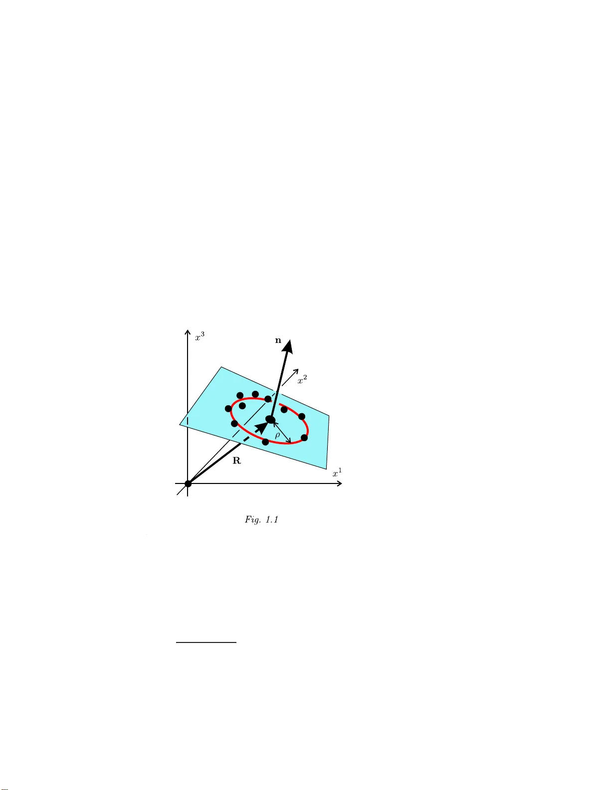
ALGORITHMS F OR LA YING POINTS OPTIMALL Y ON A PLA NE AND A CIR CLE. R. A. Sharipo v A bs tr act . Two a veraging algorithms are considered which are i n tended for choosing an opt imal plan e and an optimal cir cle approx imating a group of p oints in three- dimensional Euclidean space. 1. Introduction. Assume that in the three- dimensional Euclidean space E w e hav e a group of po in ts visually re s em bling a circle (see Fig. 1.1). The problem is to find the b e s t plane and the b est cir cle approximating this group of points. An y plane in E is given by t he equation ( r , n ) = D, (1.1) where n is the normal vector of the plane and D is some constant. The vector r in ( 1.1 ) is the radius-vector of a p oin t on that plane, while ( r , n ) is the s calar pro - duct of the vectors r and n . Once a plane ( 1.1 ) is fixed and r is the radius-vector o f so me p oint on it, a cir cle on this plane is given by the equation | r − R | = ρ. (1.2) Here ρ is the r adius o f the circle ( 1.2 ) and R is the ra dius-vector o f its cent er. Having a gr oup of p oints r [1 ] , . . . , r [ N ] in E , our goa l is to des ign an a lgorithm for ca lculating the par ameters n , D , R , and ρ in ( 1.1 ) and ( 1.2 ) thus defining a plane and a circle b eing optimal approximations of our p oints in some definite sens e. 2. Defining an optimal plane. Assume that n is a unit vector, i. e | n | = 1, and ass ume that we hav e some plane defined by the eq ua tion ( 1.1 ). Then the distance from the p oint r [ i ] to this pla ne 2000 Mathematics Subject Classific a tion . 62H35, 62P30, 68W25. Ty p eset b y A M S -T E X 2 R. A. SHARIPO V is g iv en by the following well-known formula: d [ i ] = | ( r [ i ] , n ) − D | | n | = | ( r [ i ] , n ) − D | . (2.1) If we denote b y d the ro ot of mean squa re o f the quantities ( 2.1 ), then we hav e d 2 = 1 N N X i =1 d [ i ] 2 = 1 N N X i =1 | ( r [ i ] , n ) − D | 2 . (2.2) Definition 2.1. A plane given b y the formula ( 1.1 ) with | n | = 1 is ca lled a n optimal ro ot me an squar e plane if the qua n tity ( 2.2 ) takes its minimal v alue. It is easy to s ee that d 2 in ( 2.2 ) is a function o f tw o pa rameters: n and D . It is a quadratic function of the para meter D . Indeed, we have d 2 = D 2 − 2 N N X i =1 ( r [ i ] , n ) D + 1 N N X i =1 ( r [ i ] , n ) 2 . (2.3) The qua dratic po lynomial in the right hand side o f ( 2.3 ) takes its minimal v alue if D = 1 N N X i =1 ( r [ i ] , n ) . (2.4) Substituting ( 2.4 ) back into the formula ( 2.3 ), we o btain d 2 = 1 N N X i =1 ( r [ i ] , n ) 2 − 1 N N X i =1 ( r [ i ] , n ) ! 2 . (2.5) In the next steps we use s o me mechanical analog ie s. If we place unit masses m [ i ] = 1 at the p oints r [1] , . . . , r [ N ], then the vector r cm = 1 N N X i =1 r [ i ] (2.6) is the r a dius-vector o f the center of mass . In terms of this radius vector the formu la ( 2.6 ) for D is wr itten as fo llo ws: D = ( r cm , n ) . (2.7) Now remember that the inertia tensor for a system of point masses m [ i ] = 1 is defined a s a quadratic for m g iv en by the for m ula: I ( n , n ) = N X i =1 | r [ i ] | 2 | n | 2 − N X i =1 ( r [ i ] , n ) 2 (2.8) (see [ 1 ] for more details). W e shall take the inertia tens o r relative to the center o f ALGORITHMS FOR LA YING POINTS . . . 3 mass. Therefore, we substitute r [ i ] − r cm for r [ i ] into the formula ( 2.8 ). As a result we get the following expres sion for I ( n , n ): I ( n , n ) = N X i =1 | r [ i ] − r cm | 2 | n | 2 − N X i =1 ( r [ i ] − r cm , n ) 2 . (2.9) Each quadr atic form in a three-dimensio na l Euclidean space has 3 scalar inv ariants. One of them is tra ce the inv ariant. In the c a se of the q ua dratic form ( 2.9 ), the trace inv ariant is given by the following formula: tr( I ) = 2 N X i =1 | r [ i ] − r cm | 2 . (2.10) Combining ( 2.9 ) a nd ( 2.10 ), we write I ( n , n ) = tr( I ) 2 | n | 2 − N X i =1 ( r [ i ] − r cm , n ) 2 . (2.11) T aking into account the formula ( 2.6 ), we transfo rm ( 2.1 1 ) as follows: I ( n , n ) = tr( I ) 2 | n | 2 − N X i =1 ( r [ i ] , n ) 2 + N ( r cm , n ) 2 . (2 .12) Comparing ( 2.12 ) with ( 2.5 ) and a gain ta king into a ccoun t ( 2.6 ), we get d 2 = tr( I ) 2 N | n | 2 − I ( n , n ) N . (2.13) The fo r m ula ( 2.13 ) means that d 2 is a quadr atic form s imilar to the inertia tensor. W e call it the non-flatness form and denote Q ( n , n ): Q ( n , n ) = tr( I ) 2 N | n | 2 − I ( n , n ) N = = 1 N N X i =1 ( r [ i ] , n ) 2 − 1 N N X i =1 ( r [ i ] , n ) ! 2 . (2.14) Like the inertia fo rm ( 2.9 ), the non- flatness fo r m ( 2.14 ) is p ositive, i. e. Q ( n , n ) > 0 for n 6 = 0 . If the inertia tenso r is brought to its prima ry axes, i. e. if it is diagona lized in some orthonor mal basis, then the form ( 2.14 ) diago na lizes in the same bas is. Theorem 2.1 . A plane is an optimal r o ot me an squar e plane for a gr oup of p oints if and only if it p asses thr ough the c enter of mass of these p oints and if its normal ve ct or n is dir e cte d along a primary axis of the non-flatn ess form Q of these p oints c orr esp onding to its minimal eigenvalue. 4 R. A. SHARIPO V The pr oo f is derived immediately from the definitio n 2.1 due to the formula ( 2.7 ) and the formula d 2 = Q ( n , n ). Theorem 2 . 2. An optimal r o ot me an squar e plane for a gr oup of p oints is unique if and only if the minimal eigenvalue λ min of their non-flatness form Q is distinct fr om t wo other eigenvalues, i. e. λ min = λ 1 < λ 2 and λ min = λ 1 < λ 3 . 3. Defining an optimal circle. Having found an optimal ro ot mea n squar e plane fo r the p oints r [1] , . . . , r [ N ], we c an replace them by their pro jections o n to this pla ne: r [ i ] 7→ r [ i ] − (( r [ i ] , n ) − D ) n . (3.1) Our nex t go al is to find an optimal cir cle approximating a g roup of p oints lying on some plane ( 1.1 ). L e t r [1] , . . . , r [ N ] b e their radius-vectors. The deflection of the po in t r [ i ] from the cir cle ( 1.2 ) is characterized by the following quantit y: d [ i ] = || r [ i ] − R | 2 − ρ 2 | . (3.2) Like in the case of ( 2.1 ), we denote by d the r oo t mean s quare of the quantities ( 3.2 ). Then we get the following formula: d 2 = 1 N N X i =1 d [ i ] 2 = 1 N N X i =1 ( | r [ i ] − R | 2 − ρ 2 ) 2 . (3.3) The quantit y d 2 in ( 3.3 ) is a function o f tw o parameter s: R and ρ 2 . With r espect to ρ 2 it is a quadr atic p olynomial. Indeed, we hav e d 2 = ( ρ 2 ) 2 − 2 ρ 2 N N X i =1 | r [ i ] − R | 2 + 1 N N X i =1 | r [ i ] − R | 4 . (3.4) Being a quadr atic p olynomial of ρ 2 , the quantit y d 2 takes its minimal v alue for ρ 2 = 1 N N X i =1 | r [ i ] − R | 2 . (3.5) Substituting ( 3.5 ) back into the formula ( 3.4 ), we der iv e d 2 = 1 N N X i =1 | r [ i ] − R | 4 − 1 N N X i =1 | r [ i ] − R | 2 ! 2 . (3.6) Upo n expanding the expr ession in the r igh t hand side of the formula ( 3.6 ) we need to p erfor m s ome simple, but ra ther huge ca lculations. As res ult we g et d 2 = 1 N N X i =1 | r [ i ] | 4 − 1 N N X i =1 | r [ i ] | 2 ! 2 − 4 N N X i =1 | r [ i ] | 2 ( r [ i ] , R ) + ALGORITHMS FOR LA YING POINTS . . . 5 + 4 1 N N X i =1 | r [ i ] | 2 ! 1 N N X i =1 ( r [ i ] , R ) ! + 4 N N X i =1 ( r [ i ] , R ) 2 − 4 1 N N X i =1 ( r [ i ] , R ) ! 2 . W e see that the ab ov e expres sion is no t higher tha n quadratic with resp ect to R . The fourth order terms and the cubic ter ms are canceled. Note a lso that the quadratic part o f the ab ov e expr ession is determined by the for m Q considered in previous sectio n. F or this reason we write d 2 as d 2 = 4 Q ( R , R ) − 4 ( L , R ) + M . (3.7) The vector L and the scalar M in ( 3.7 ) are given by the following formulas: L = 1 N N X i =1 | r [ i ] | 2 ( r [ i ] − r cm ) , (3.8) M = 1 N N X i =1 | r [ i ] | 4 − 1 N N X i =1 | r [ i ] | 2 ! 2 . (3.9) The quantit y d 2 takes its minimal v alue if and only if R satisfies the equation 2 Q ( R ) = L , (3.10) where Q is the symmetric linear op erator ass ocia ted with the for m Q through the standard Euclidea n s calar pro duct. The equality ( Q ( X ) , Y ) = Q ( X , Y ) , which s ho uld b e fulfilled for arbitrar y tw o vectors X a nd Y , is a for ma l definition of the op erator Q (see [ 2 ] for more deta ils). In genera l case the op erator Q is non-degenera te. Hence, R do es exist and uniquely fix ed by the equation ( 3.10 ). Ho wev er, if the p oin ts r [1] , . . . , r [ N ] are laid onto the plane ( 1.1 ) by means of the pro jection pro cedure ( 3.1 ), then the op erator Q is degenera te. Mo reov er, one can prove the following theor em. Theorem 3 . 1. The non-flatn ess form Q and its asso ciate d op er ator Q ar e de gen- er ate if and only if the p oints r [1 ] , . . . , r [ N ] lie on some plane. In this flat case pr ovided b y the theorem 3.1 one should mov e the orig in to that plane where the p oints r [1 ] , . . . , r [ N ] lie and treat their r adius-vectors as t wo-dimensional vectors. Then, us ing ( 2.14 ), ( 3 .8 ), and ( 3.9 ), one should rebuild the tw o-dimensional versions of the non-flatness form Q , its asso ciated op erato r Q and the par ameters L a nd M . If aga in the tw o-dimensiona l non-flatness for m is degenerate, this case is describ ed by the following theor e m. Theorem 3.2. The two-dimensional non-flatness form Q and its asso ciate d op- er ator Q ar e de gener ate if and only if al l of t he p oints r [1] , . . . , r [ N ] lie on some str aight line. In this very sp ecial cas e we say tha t str aight line a ppr oximation for the p oint s r [1] , . . . , r [ N ] is more prefer able tha n the circular appr o ximation. Note that the same decision can b e ma de in so me cases even if the p oint s r [1] , . . . , r [ N ] do not 6 R. A. SHARIPO V lie o n o ne straight line ex a ctly . If tw o eigenv alue s o f the three-dimensional non- flatness form Q are sufficiently small, i. e. if they b oth are muc h sma ller than the third eig en v alue of this form, then we can say that λ min ≈ λ 1 , λ min ≈ λ 2 . T aking tw o eige n vectors n 1 and n 2 of the for m Q co rresp onding to the eig e n v a lues λ 1 and λ 2 , we define t wo planes ( r , n 1 ) = D 1 , ( r , n 2 ) = D 2 . (3.11) The constants D 1 and D 2 in ( 3.11 ) ar e given by the formula ( 2.7 ). The inter- section of t wo pla nes ( 3.11 ) y ie lds a str aight line b eing the optimal straight line approximation fo r the po in ts r [1] , . . . , r [ N ] in this ca se. 4. Ackno wledgments. The idea of this pap er was induced by s ome tec hnologic a l problems sugg ested to me by O. V. Agee v. I am grateful to him for that. References 1. Landau L. D., Lif shits E. M., Course of the or etic al physics, V ol. I , Me chanics , Nauk a pub- lishers, Mosco w, 1988. 2. Shari pov R. A, Course of linea r algebr a and multidimensional g e ometry , Bashkir State Uni- v ersity , Ufa, 1996; see also math.HO/0405323 . 5 R a bo c ha ya st re et , 4 5 0 0 03 U f a, R us si a C ell P h on e: + 7- (9 1 7) -4 7 6- 93 -4 8 E-mail addr ess : r-sharip ov@mail.ru R Sharipov @ic.bashedu. ru URL : http:/ /www.geo cities.com/r-sharipov http:/ /w ww.freetext books.boom.ru/index.html