Deep learning methods-physics-informed neural networks (PINNs), deep operator networks (DeepONet), and graph network simulators (GNS)-are increasingly proposed for geotechnical problems. This paper tests these methods against traditional solvers on canonical problems: wave propagation and beam-foundation interaction. PINNs run 90,000 times slower than finite difference with larger errors. DeepONet requires thousands of training simulations and breaks even only after millions of evaluations. Multi-layer perceptrons fail catastrophically when extrapolating beyond training data-the common case in geotechnical prediction. GNS shows promise for geometryagnostic simulation but faces scaling limits and cannot capture path-dependent soil behavior. For inverse problems, automatic differentiation through traditional solvers recovers material parameters with sub-percent accuracy in seconds. We recommend: use automatic differentiation for inverse problems; apply site-based cross-validation to account for spatial autocorrelation; reserve neural networks for problems where traditional solvers are genuinely expensive and predictions remain within the training envelope. When a method is four orders of magnitude slower with less accuracy, it is not a viable replacement for proven solvers.
Machine learning (ML) methods are increasingly proposed as replacements for traditional geotechnical analyses, promising instant predictions that bypass expensive solvers (Durante and Rathje, 2021;Hudson et al., 2023;Geyin and Maurer, 2023;Ilhan et al., 2025). Applications now common in geotechnical journals include physics-informed neural networks (PINNs) for wave propagation and deep operator networks (DeepONet) for foundation response. The promise is compelling: train a model once on past case histories, then predict instantly for new conditions. But should we believe this promise? More precisely, under what conditions does machine learning genuinely outperform the traditional methods we have refined over decades?
This paper answers that question through direct numerical comparison. We “stress-test” these ML methods against traditional solvers, applying them to the same canonical problems and measuring wall-clock time, accuracy, and ease of implementation. We focus on simple one-dimensional problems-like wave propagation and consolidation-for the same reason Terzaghi started with 1D consolidation: the physics is crystal clear, exact solutions exist, and they are the building blocks of more complex analyses. While traditional solvers are already exceptionally fast in 1D, these simple tests are essential. They allow us to establish a clear performance baseline, exposing a method’s fundamental limitations, relative computational overhead, and failure modes. If a method proves inaccurate or orders of magnitude slower than its traditional counterpart on a 1D problem, we must understand why before trusting it on complex 3D problems where such validation is nearly impossible.
This work provides the quantitative evidence for the significant challenges-such as data requirements, physical consistency, and extrapolation reliability-that recent reviews have acknowledged (Wang et al., 2025;Fransen et al., 2025). This is not a dismissal of machine learning, but a call for the same validation standards we apply to any other engineering tool, from concrete testing to slope stability analysis. We argue that we should not replace proven solvers with neural networks without a clear, demonstrated advantage in accuracy, computational cost, or physical consistency.
The paper is structured as follows. We first establish two fundamental limitations affecting all ML methods: catastrophic extrapolation failure and the validation trap of spatial autocorrelation. We then quantify the performance of multi-layer perceptrons, PINNs, and DeepONet against their finite difference counterparts. Finally, we present an alternative that does work for inverse problems-automatic differentiation-and provide a practical decision framework for geotechnical engineers who want to use these modern computational tools effectively.
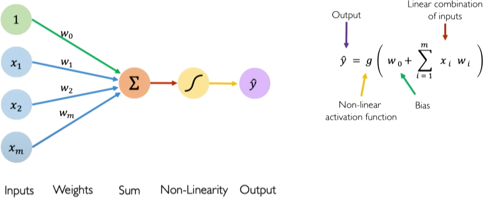
2 Multi-Layer Perceptrons in Geotechnical Engineering Multi-layer perceptrons (MLPs) are the foundation of modern neural networks. Understanding how they work clarifies why they fail in certain geotechnical applications. An MLP transforms inputs into outputs through layers of interconnected neurons. Each neuron computes a weighted sum of its inputs, adds a bias term, and passes the result through a nonlinear activation function (fig. 1):
where x i are inputs (e.g., depth, cone resistance, pore pressure), w i are learnable weights, w 0 is the bias, and g is the activation function.
The key insight is that only the weights and biases are trainable. The activation function g is fixed-chosen before training and never modified. This means the network learns by adjusting linear combinations; all nonlinearity comes from the fixed activation function applied to these linear combinations. Training minimizes a loss function measuring prediction error. For regression, the mean squared error is typical:
Figure 1: A single neuron (perceptron) computes a weighted sum of inputs plus bias, then applies a nonlinear activation function g. Stacking neurons into layers creates a multi-layer perceptron capable of approximating complex nonlinear relationships.
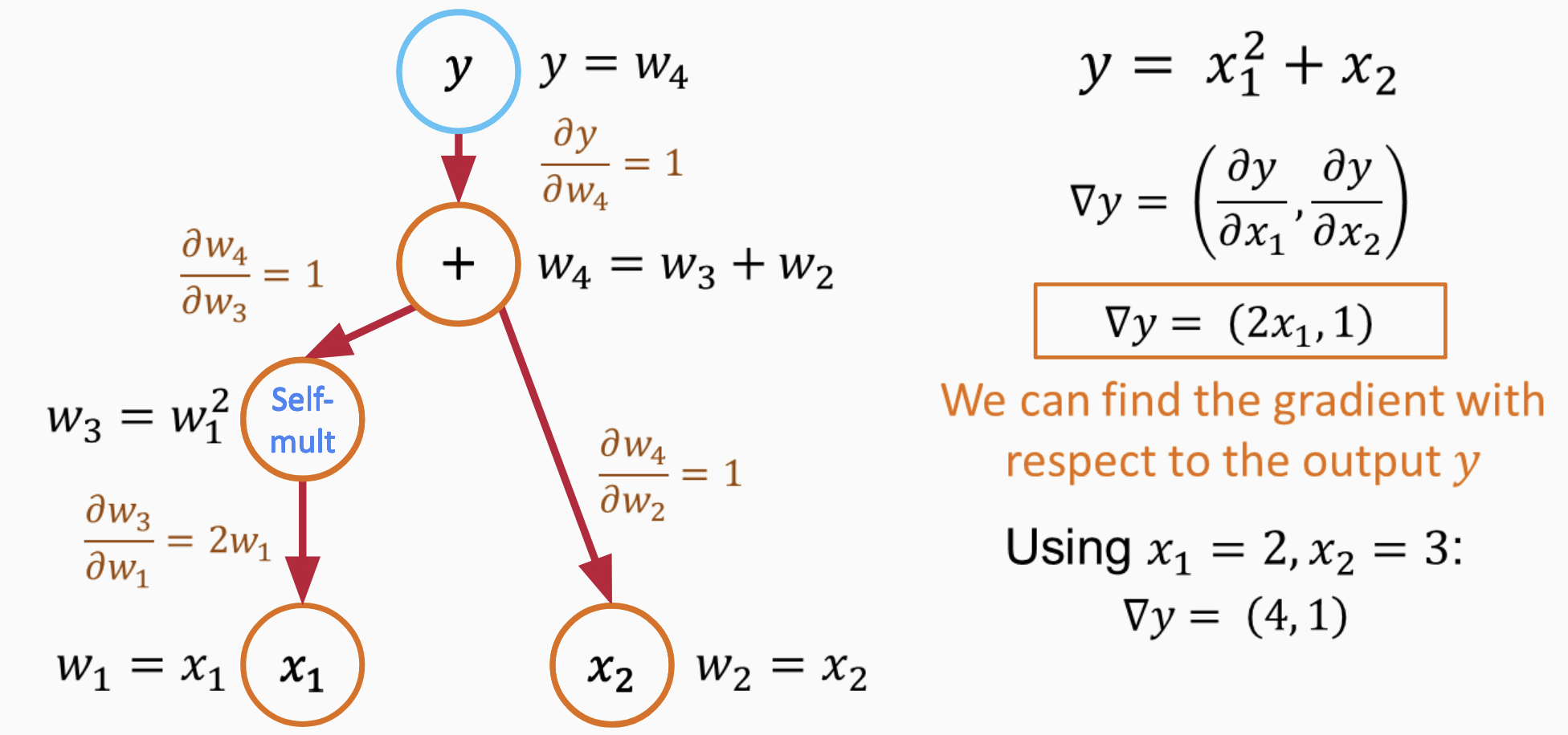
Weights update iteratively via gradient descent, w ← w -η∇ w L, where η is the learning rate. Backpropagation computes these gradients efficiently by applying the chain rule layer by layer, working backward from output to input. Stacking neurons into multiple layers allows the network to learn hierarchical features, with early layers capturing simple patterns and deeper layers combining these into complex relationships.
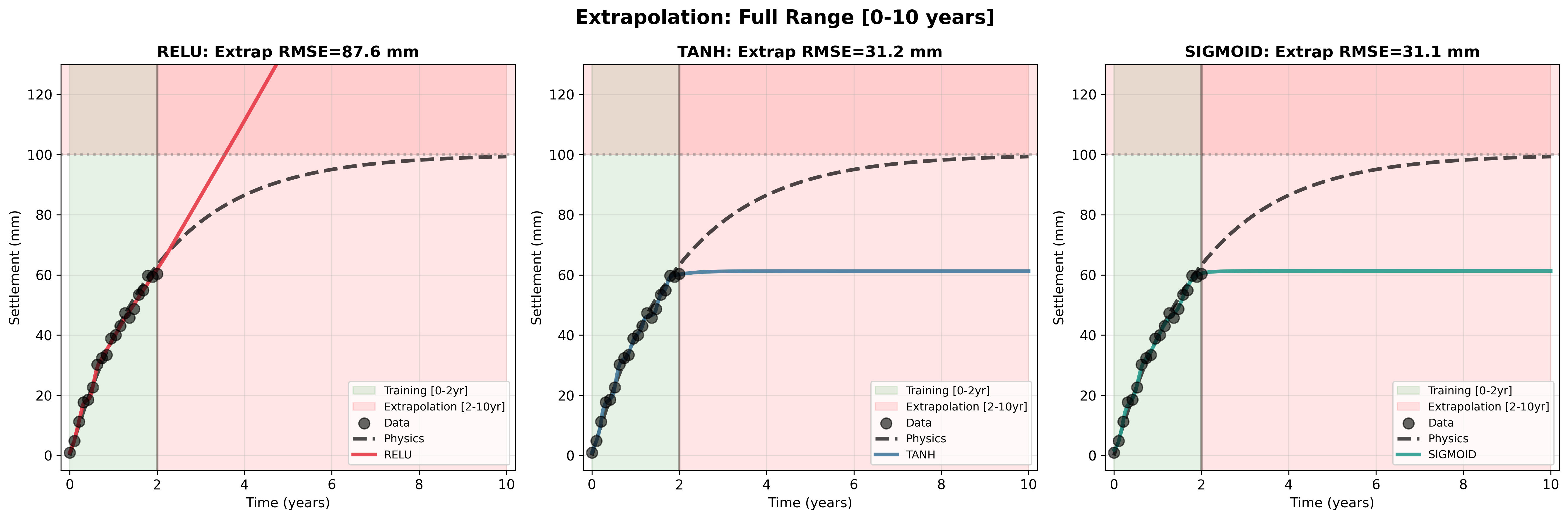
The choice of activation function determines how the network represents nonlinearity. Common options include ReLU (g(z) = max(0, z)), tanh (g(z) = tanh(z), outputs between -1 and +1), and sigmoid (g(z) = 1/(1 + e -z ), outputs between 0 and 1). Each has a sensitive region where small changes in input produce meaningful changes in output-and a saturated region where the function flattens and gradients vanish.
For tanh and sigmoid, the sensitive region lies roughly
This content is AI-processed based on open access ArXiv data.