Adaptive optimizers such as Adam have achieved great success in training large-scale models like large language models and diffusion models. However, they often generalize worse than non-adaptive methods, such as SGD on classical architectures like CNNs. We identify a key cause of this performance gap: adaptivity in pre-conditioners, which limits the optimizer's ability to adapt to diverse optimization landscapes. To address this, we propose Anon (Adaptivity Non-restricted Optimizer with Novel convergence technique), a novel optimizer with continuously tunable adaptivity
, allowing it to interpolate between SGD-like and Adam-like behaviors and even extrapolate beyond both. To ensure convergence across the entire adaptivity spectrum, we introduce incremental delay update (IDU), a novel mechanism that is more flexible than AMSGrad's hard max-tracking strategy and enhances robustness to gradient noise. We theoretically establish convergence guarantees under both convex and non-convex settings. Empirically, Anon consistently outperforms state-of-the-art optimizers on representative image classification, diffusion, and language modeling tasks. These results demonstrate that adaptivity can serve as a valuable tunable design principle, and Anon provides the first unified and reliable framework capable of bridging the gap between classical and modern optimizers and surpassing their advantageous properties.
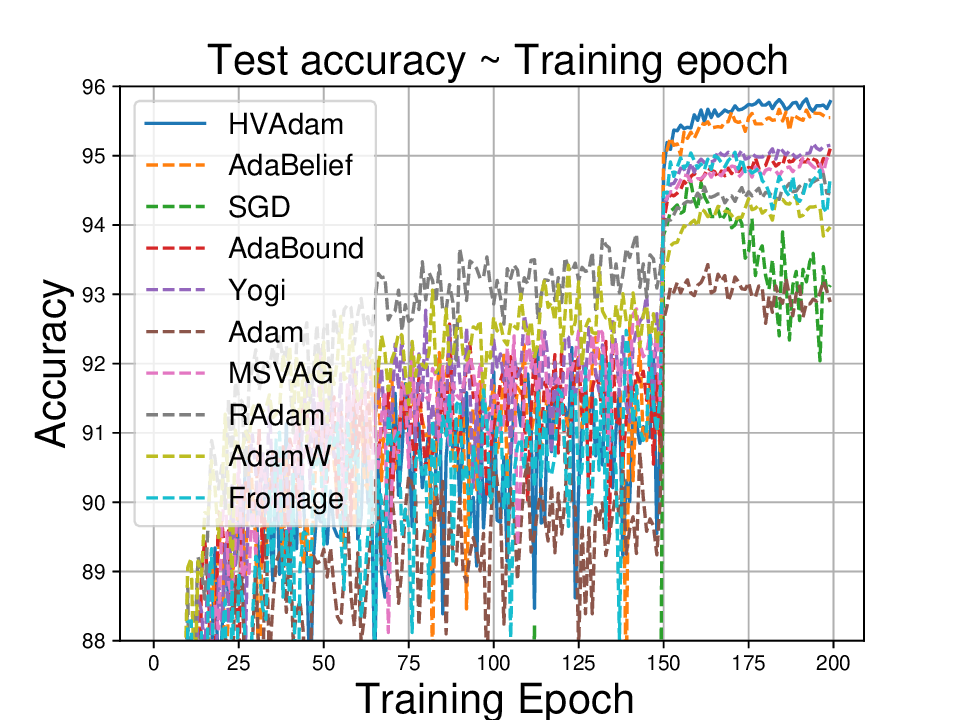
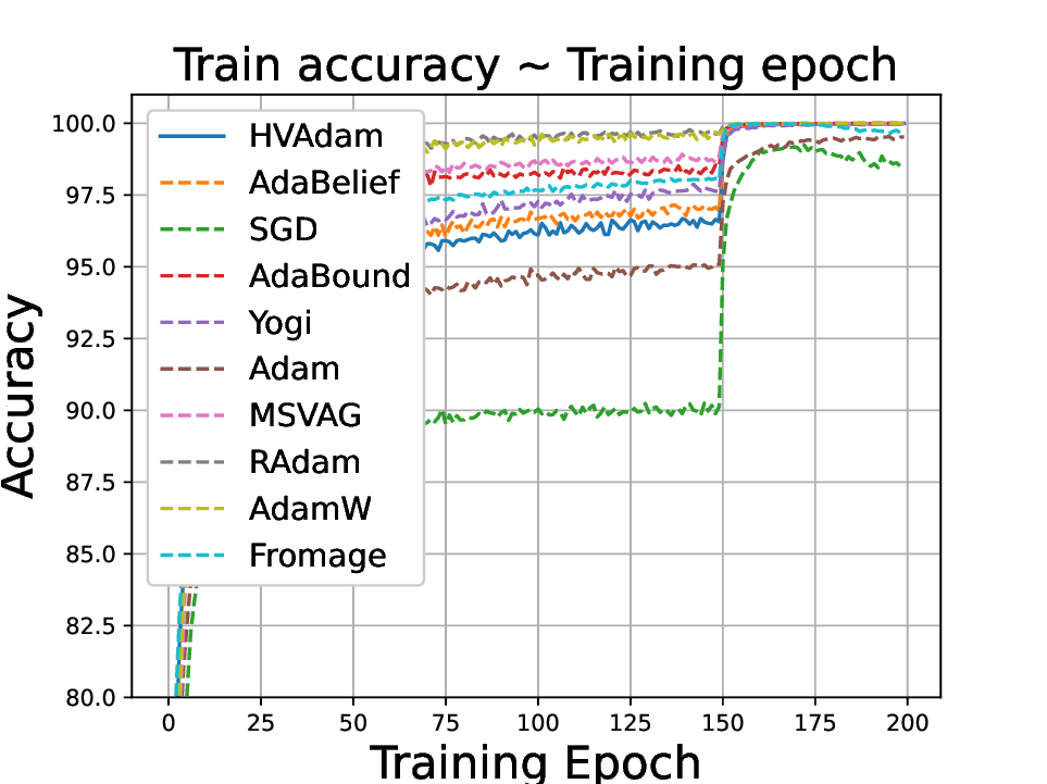
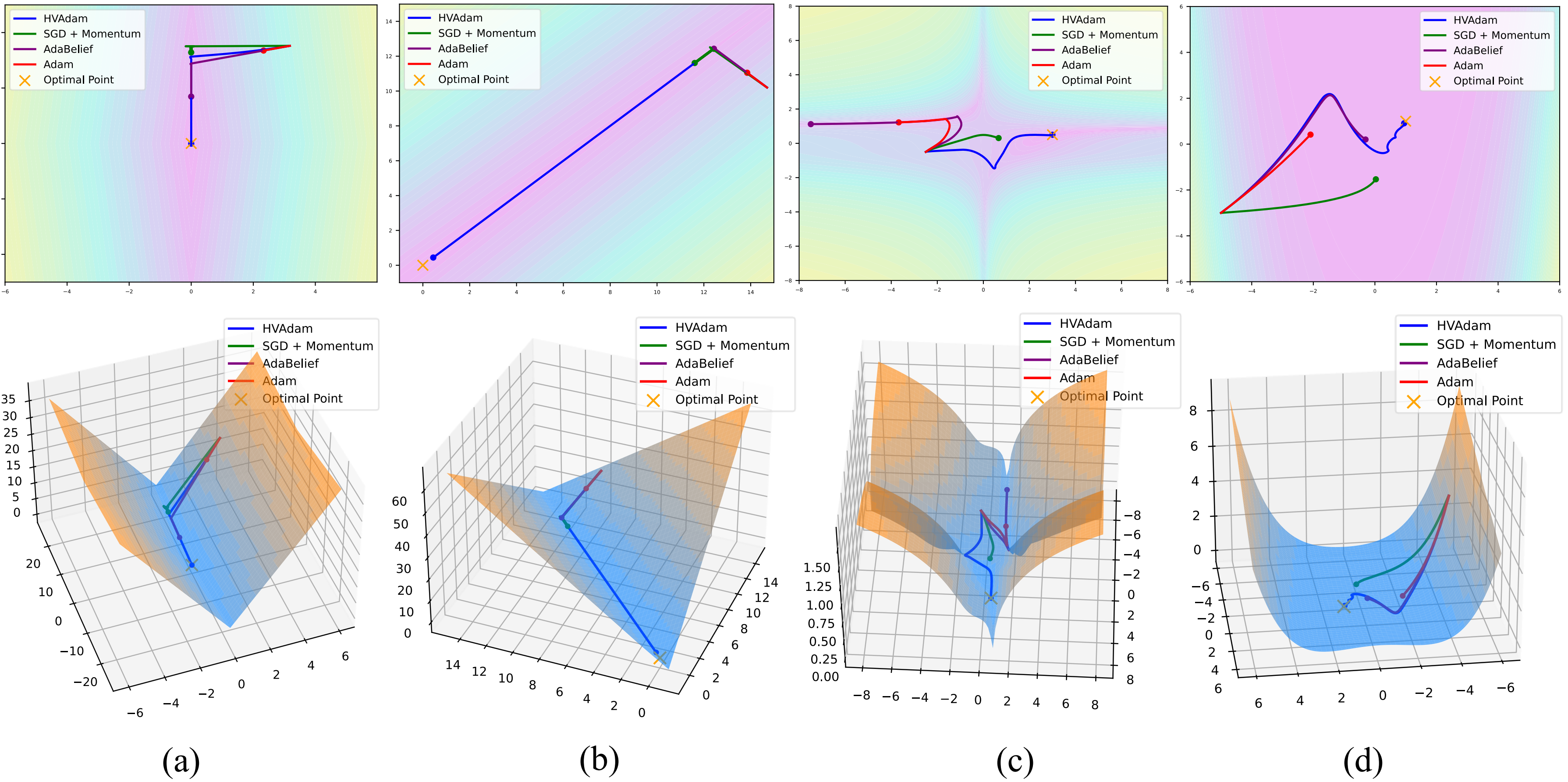
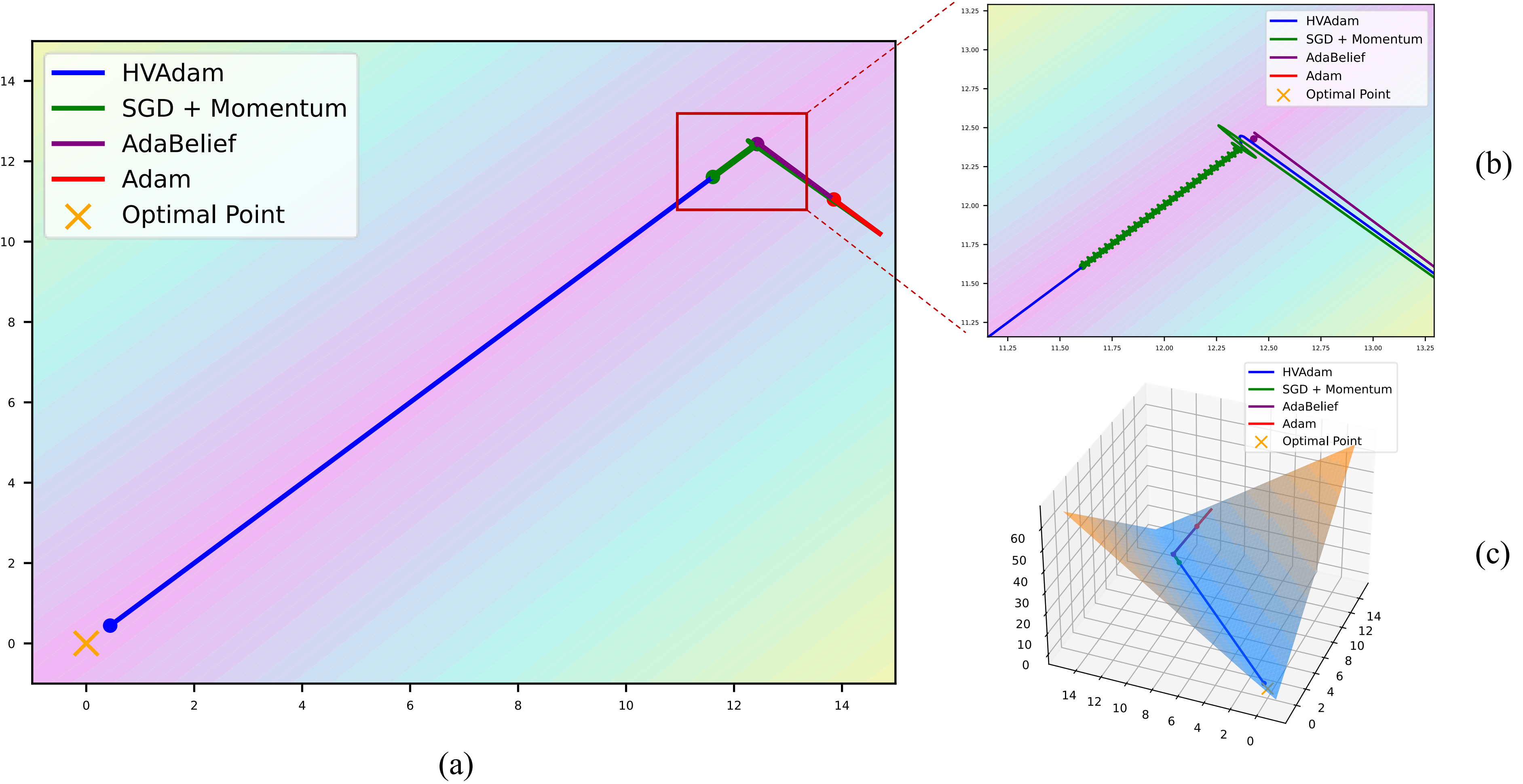
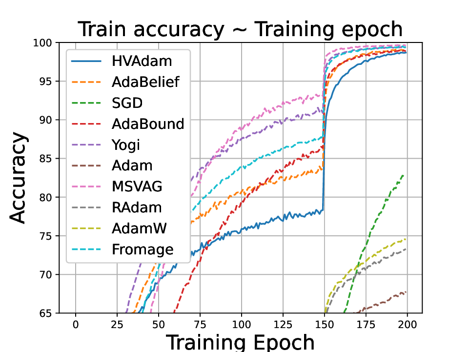
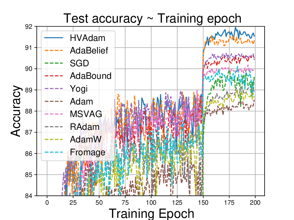
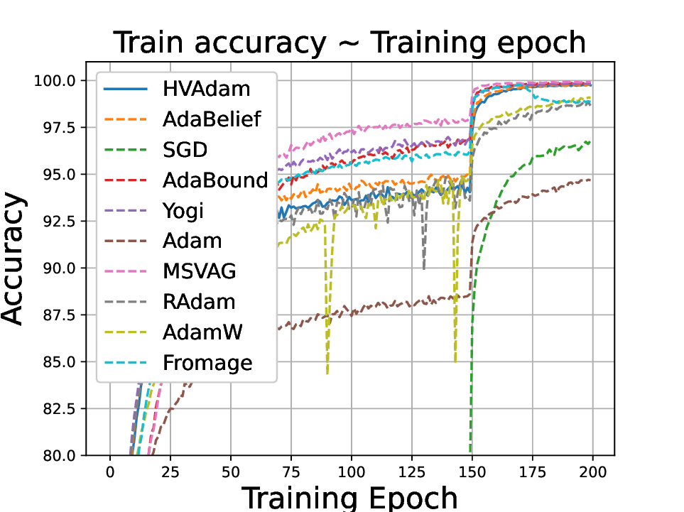
Optimizers play a crucial role in machine learning, efficiently minimizing loss and achieving generalization. There are two main types of state-of-the-art optimizers: Nonadaptive optimizers, for instance, stochastic gradient descent (SGD) (Robbins and Monro 1951), use a global learning rate for all parameters. In contrast, adaptive optimizers, such as RMSProp (Graves 2013) and Adam (Kingma and Ba 2014), use the partial derivative of each parameter to adjust their learning rates separately. When applied correctly, adaptive optimizers can significantly accelerate the convergence of parameters, even in cases where partial derivatives are minimal. These adaptive optimizers are crucial for overcoming saddle points or navigating regions characterized by small partial derivatives, which can otherwise hinder the convergence process (Xie et al. 2022). In deep learning, model parameters often change significantly during training, and these changes frequently reverse direction, especially when the model is getting close to its optimal performance (near the minimum of the loss function). Adam dynamically adjusts the learning rate according to the magnitude of the gradients, while SGD incorporates momentum to smooth the gradient and does not directly modify the learning rate. AdaBelief (Zhuang et al. 2020), a variant of Adam, adjusts the learning rate based on the deviation of the gradient from the moving average. However, these approaches may be problematic in complex landscapes, such as valley-like regions that are quite common within the loss functions of deep learning models (Zhuang et al. 2020). In such regions, the true direction of optimization often has a small gradient, making it difficult for traditional optimizers to identify and efficiently optimize in these directions. Traditional optimizers tend to oscillate along valley sides, where gradients are larger, leading to slow and inefficient convergence. We refer to this phenomenon as the Valley Dilemma, which occurs when optimization techniques fail to converge effectively due to the challenging landscape as shown in Figure 1.
To further demonstrate the Valley Dilemma, we illustrate its effect on optimizers using two more common loss functions (e.g., (c) and (d) in Figure 2). In valley-like regions, traditional optimizers face several key challenges: 1. Identifying Update Direction: In valley-like regions, the true optimal direction (along the valley floor) often has a very small gradient, making it difficult for traditional optimizers to detect and follow this direction, as shown in Figure 1. 2. Changing Landscapes: As training progresses, the direction of optimization can change, as shown in Figure 2(b)(c), especially in complex and dynamic landscapes. 3. Adjusting Learning Rate: Since this stable update direction incorporates trend information, the learning rate needs to be adjusted accordingly. To help convergence in other directions, we should design a more reasonable learning rate adjustment strategy based on the information of the trend for them.
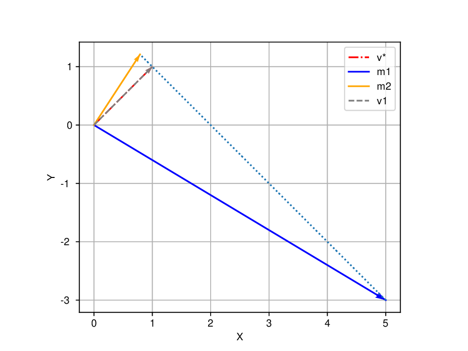
To address the aforementioned challenges, we propose the hidden-vector-based adaptive gradient method (HVAdam), an adaptive optimizer that considers the full dimensions of the parameters. With the help of the hidden vector, HVAdam can determine the stable update direction, which enables faster convergence along the descending trajectory of the loss function through an increased learning rate compared to the traditional zigzag approach. Additionally, HVAdam employs a restart strategy to adapt the change of the hidden vector, namely the changing direction of the landscapes. Lastly, HVAdam incorporates information from all dimensions to adjust the learning rate for each dimension using a new preconditioning matrix based on the hidden vector. Contributions of our paper can be summarized as follows:
• We propose HVAdam, which constructs a vector that ap-proximates the invariant components within the gradients, namely the hidden vector, to more effectively guide parameter updates as a solution to the Valley Dilemma.
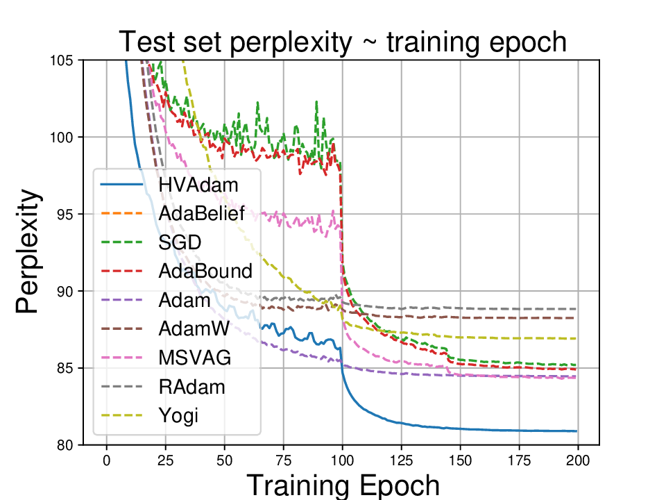
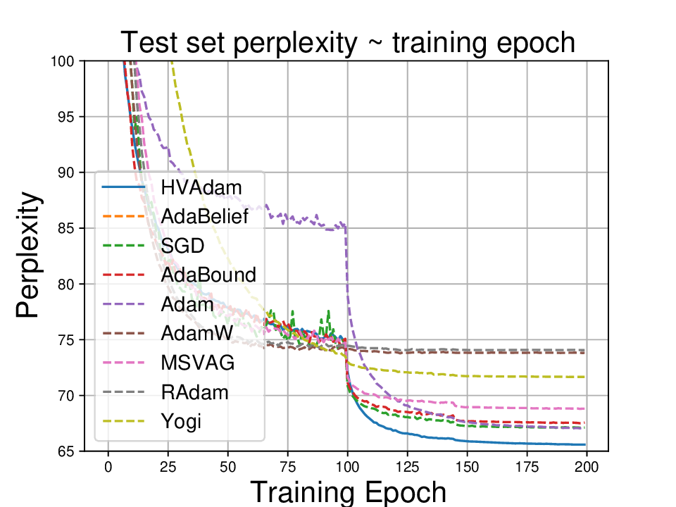
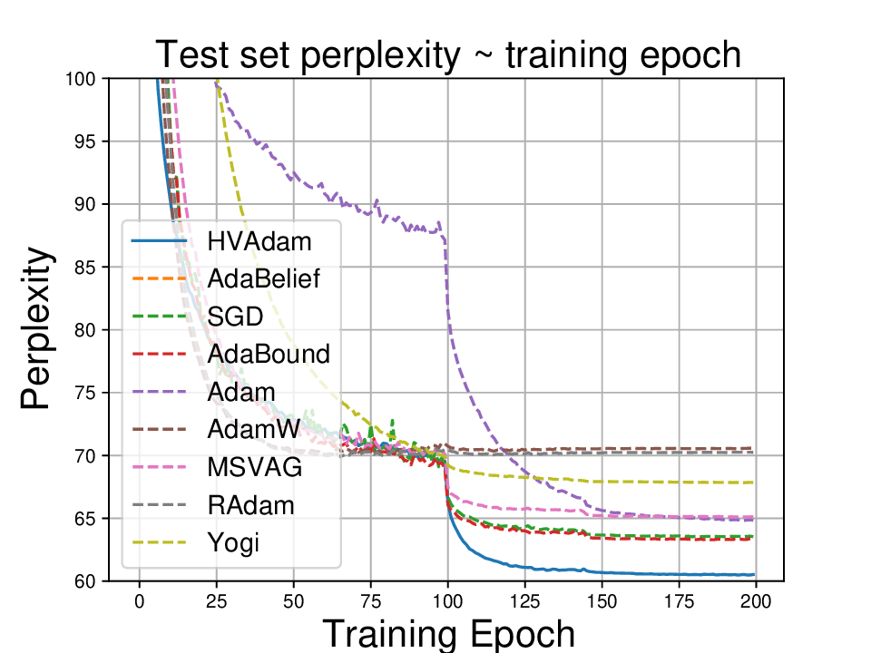
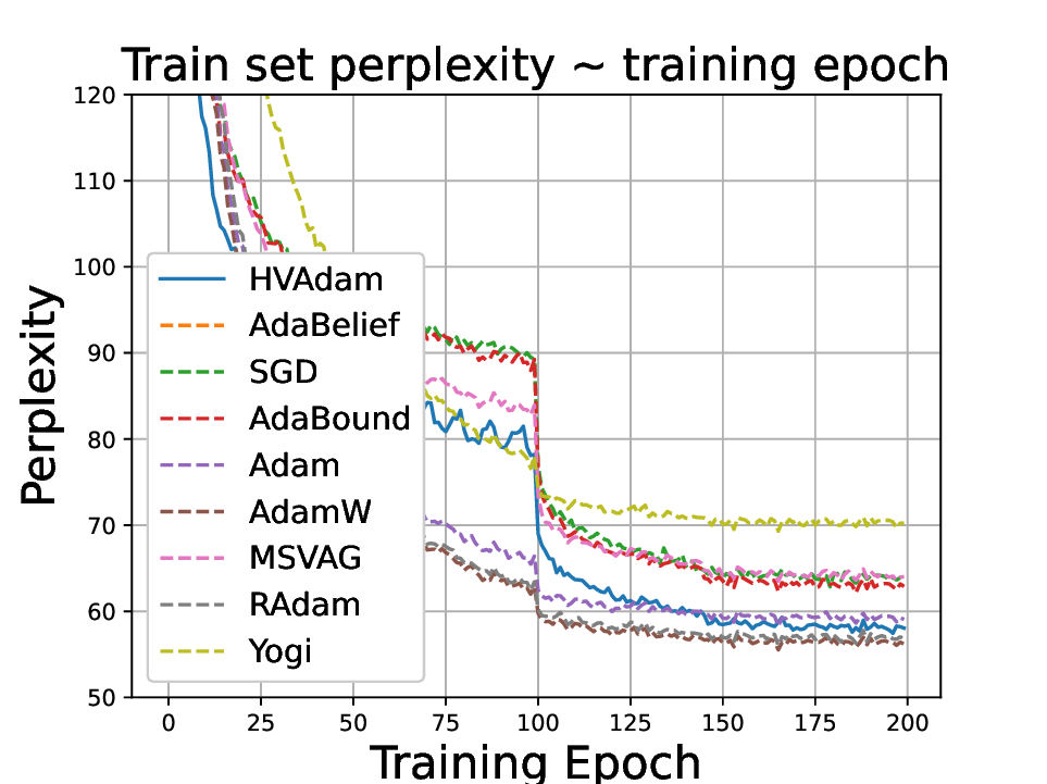
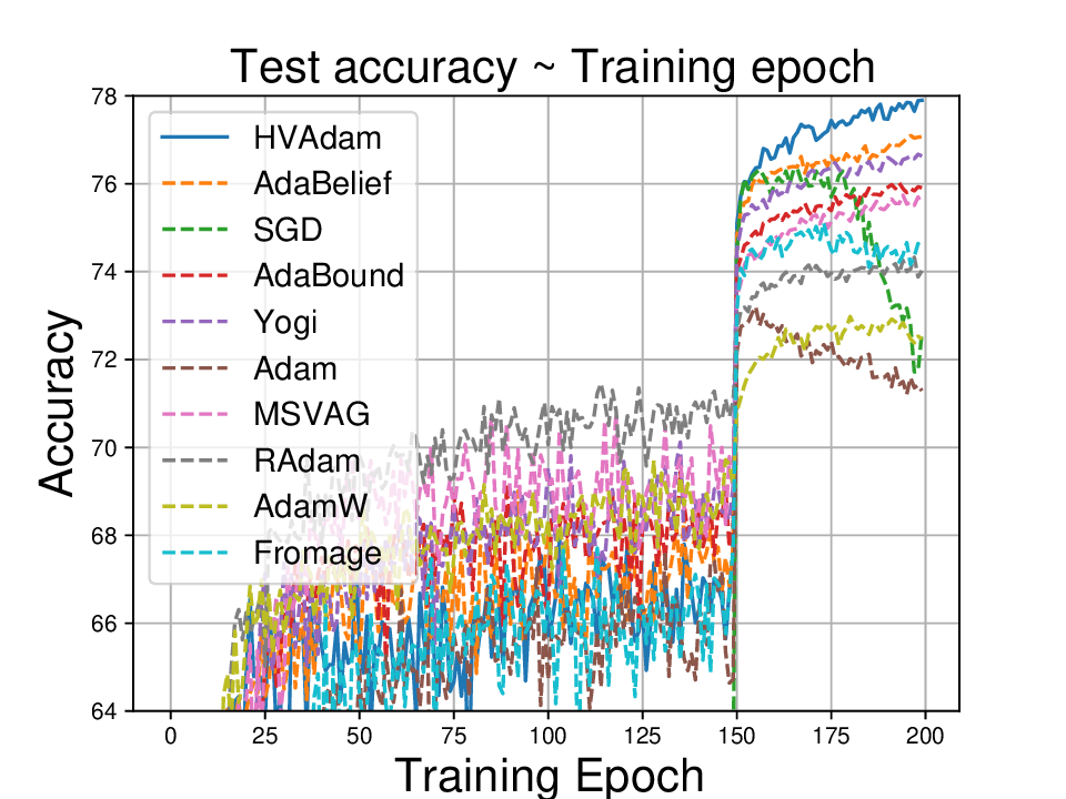
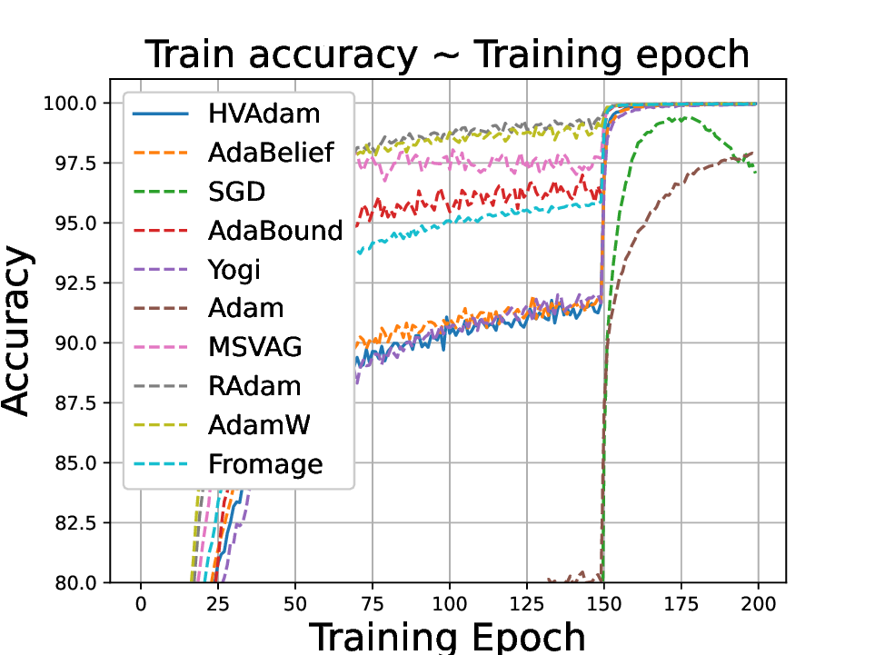
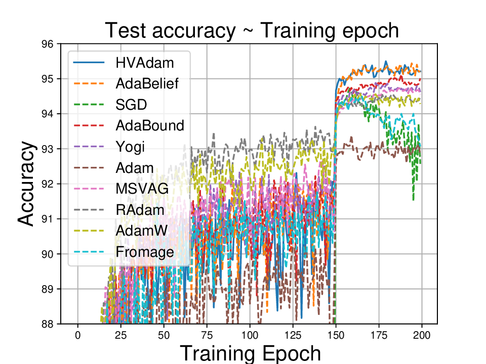
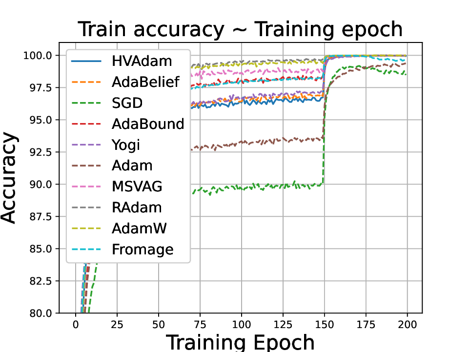
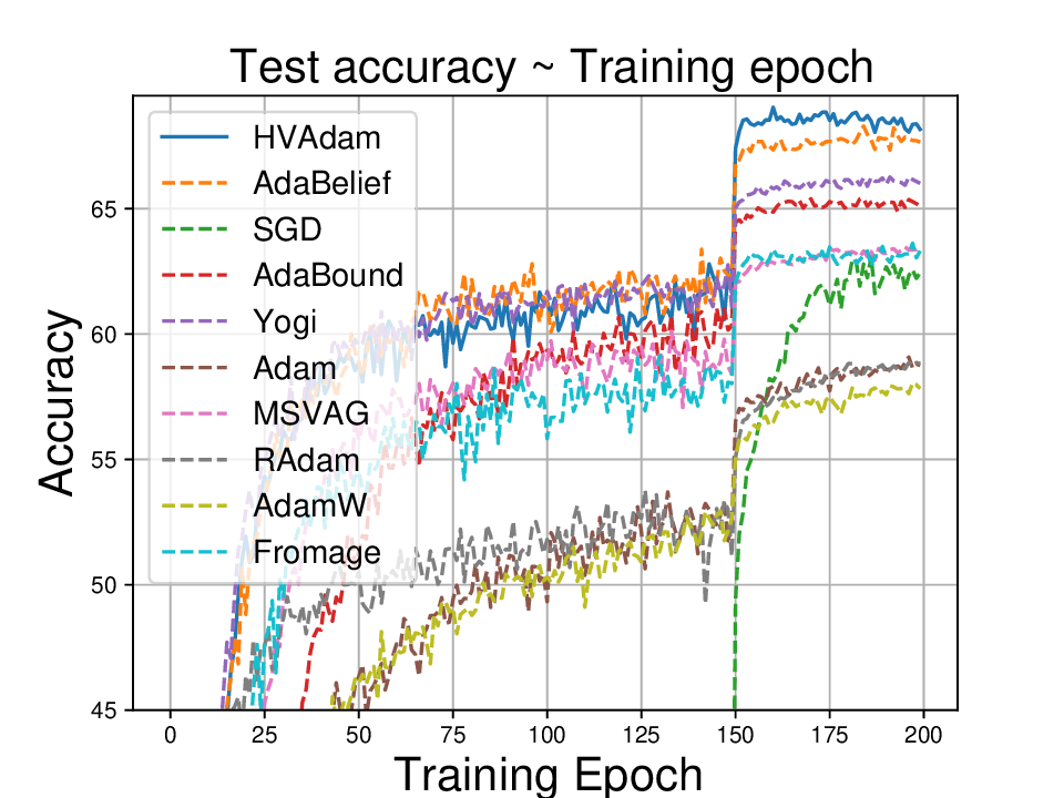
• We demonstrate HVAdam’s convergence properties under online convex and non-convex stochastic optimization, emphasizing its efficacy and robustness. • We empirically evaluate the performance of HVAdam, demonstrating its significant improvements across image classification, NLP, and GANs tasks.
is the scalar-valued function to minimize, θ is the parameter in R d to be optimal.
α 2 is the unadjusted learning rate for v t ; γ is a constant to limit the value of η t , which is usually set as 0. These are hyperparameters. • δ t ∈ R: The factor used to adjust α 2t .
• ϵ ∈ R: The hyperparameter ϵ is a small number, used for avoiding division by 0.
• lr(δ t2 , δ t2 ) ∈ R×R → R:
The function can be set as other more suitable choices; we will not change it in the rest of the paper unless otherwise specified. • β 1 , β 2 ∈ R: The hyperparameter for EMA, 0 ≤ β 1 , β 2 < 1, typically set as 0.9 and 0.999.
A
This content is AI-processed based on open access ArXiv data.