Ohmic Power of Ideal Pulsars

arXiv:1101.5844v1 [astro-ph.HE] 31 Jan 2011 Ohmic Power of Ideal Pulsars Andrei Gruzinov CCPP, Physics Department, New York University, 4 Washington Place, New York, NY 10003 ABSTRACT Ideal axisymmetric pulsar magnetosphere is calculated from the standard stationary force- free equation but with a new boundary condition at the equator. The new solution predicts Ohmic heating. About 50% of the Poynting power is dissipated in the equatorial current layer outside the light cylinder, with about 10% dissipated between 1 and 1.5 light cylinder radii. The Ohmic heat presumably goes into radiation, pair production, and acceleration of charges – in an unknown proportion. 1. Introduction We have shown that ideal pulsars calculated in the force-free limit of Strong-Field Electrodynam- ics (SFE) dissipate a large fraction of the Poynt- ing flux in the singular current layer outside the light cylinder (Gruzinov 2011). This result – finite damping in an ideal system – is not really that unusual. Burgers equation, for instance, with vis- cosity +0, dissipates finite energy in infinitely thin shocks. The standard axisymmetric pulsar magneto- sphere features a nearly head-on1 collision of Poynting fluxes right outside the light cylinder. It is to be expected, although merely by common sense, that such a collision should be accompanied by damping. Here we show that our SFE solution also ob- tains from the standard force-free magnetosphere equation of Scharlemant & Wagoner (1973), if one uses the “correct” boundary condition at the equa- torial current layer. We propose that the “correct” boundary condi- tion at the singular current layer (which now exists only outside the light cylinder) is B2 −E2 = 0. 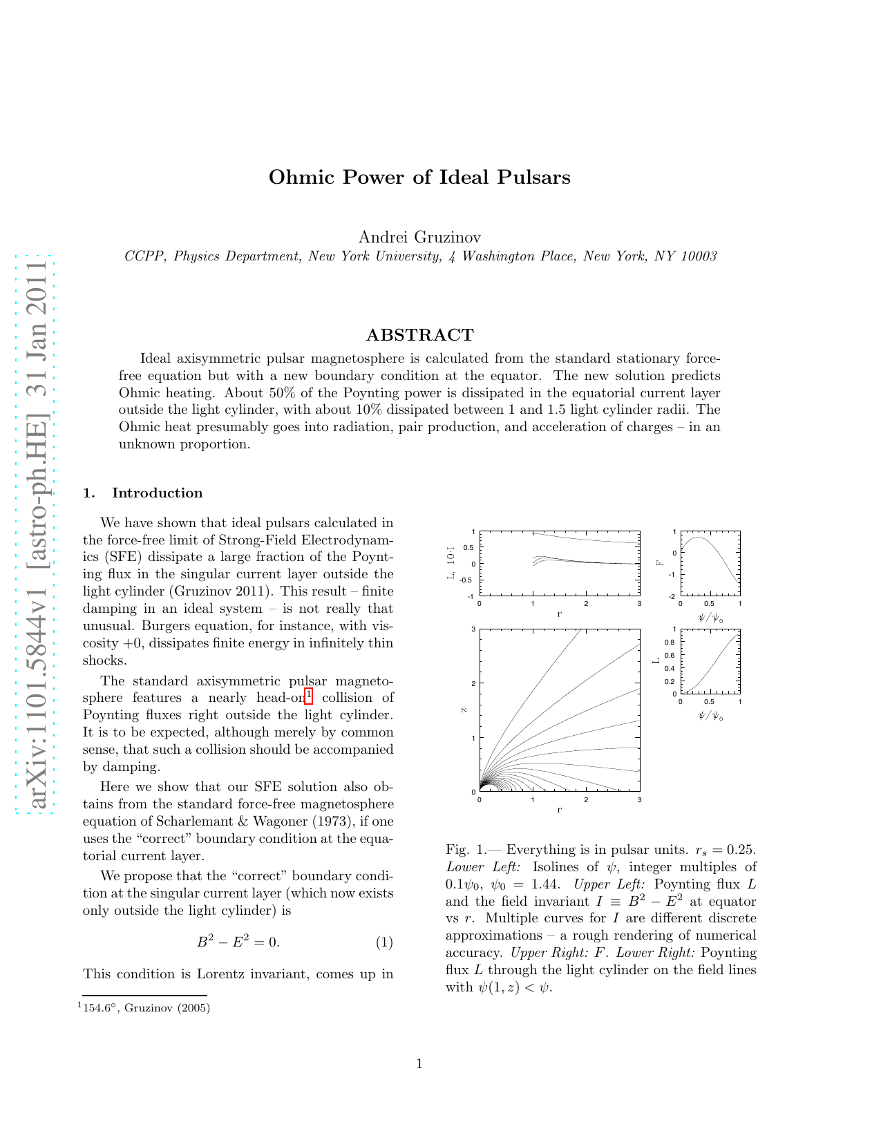(1) This condition is Lorentz invariant, comes up in 1154.6◦, Gruzinov (2005) 0 1 2 3 0 1 2 3 0 0.5 1 -2 -1 0 1 0 0.5 1 0 0.2 0.4 0.6 0.8 1 0 1 2 3 -1 -0.5 0 0.5 1 Fig. 1.— Everything is in pulsar units. rs = 0.25. Lower Left: Isolines of ψ, integer multiples of 0.1ψ0, ψ0 = 1.44. Upper Left: Poynting flux L and the field invariant I ≡B2 −E2 at equator vs r. Multiple curves for I are different discrete approximations – a rough rendering of numerical accuracy. Upper Right: F. Lower Right: Poynting flux L through the light cylinder on the field lines with ψ(1, z) < ψ. 1 the SFE simulations 2, and has a clear physical meaning (at equator, the field becomes electric- like in order to drive large current). We cannot be sure that our proposal works, un- til one justifies the full SFE, or just eq.(1), micro- scopically. But conversion of 50% of the Poynting flux into the Ohmic power (radiation, electron- positron pairs) occurring close to the light cylin- der must have consequences for the pulsar phe- nomenology, and needs to be studied. In §2 we derive the pulsar magnetosphere equa- tion and explain how Contopoulos, Kazanas & Fendt (1999) solve it. In §3 we put together all the equations which are needed to calculate the pulsar magnetosphere. In §4 we describe the numerical solution and the corresponding physics results. 2. Ideal pulsar magnetosphere Goldreich & Julian (1969) proposed that neu- tron star magnetospheres obey the force-free con- dition ρE + j × B = 0. (2) Surprisingly, it turns out that this simple equa- tions allows a full calculation of the pulsar mag- netosphere (Scharlemant & Wagoner 1973, Con- topoulos, Kazanas & Fendt 1999, Gruzinov 2005, Spitkovsky 2006). For the stationary axisymmetric case, the cal- culation is as follows. Using axisymmetry and stationarity, in cylindrical coordinates (r, θ, z), we represent the fields by the three scalars φ, ψ, and A, which depend on r and z but not on θ: E = −∇φ, B = 1 r (−ψz, A, ψr), (3) where the subscripts denote the partial deriva- tives. We plug (3) into (2) and use ρ = ∇· E and j = ∇× B. We also use the boundary conditions at the surface of the star – the continuity of the normal component of the magnetic field and the tangential component of the electric field. We use the pulsar units µ = Ω= c = 1, (4) where µ is the magnetic dipole moment of the star. It is assumed that the magnetic field is a pure 2See Fig.5 of Gruzinov (2008). dipole near the surface inside the star. The star is assumed to be a perfect conductor. Ωis the angular velocity of the star. We get φ = ψ, A = A(ψ), (5) where A is an arbitrary function of ψ, and we also get the “Grad-Shafranov-like” pulsar magne- tosphere equation for ψ (1 −r2)∆ψ −2 r ψr + F(ψ) = 0. (6) Here ∆≡∇2, and F ≡AA′, where the prime de- notes the ψ-derivative. The pulsar magnetosphere equation (6) is solved outside the star r2 + z2 > r2 s, (7) with the boundary condition at the surface of the star ψ = r2 r3s , r2 + z2 = r2 s. (8) The pulsar magnetosphere equation (6) con- tains F – an arbitrary function of ψ, and it is not clear how one should solve it. This was ex- plained and done by Contopoulos, Kazanas & Fendt (1999) (CKF). The pulsar magnetosphere equation is elliptical both inside and outside the light cylinder, and can therefore be solved

This content is AI-processed based on open access ArXiv data.