Spatial Degrees of Freedom and Channel Strength for Antenna Systems

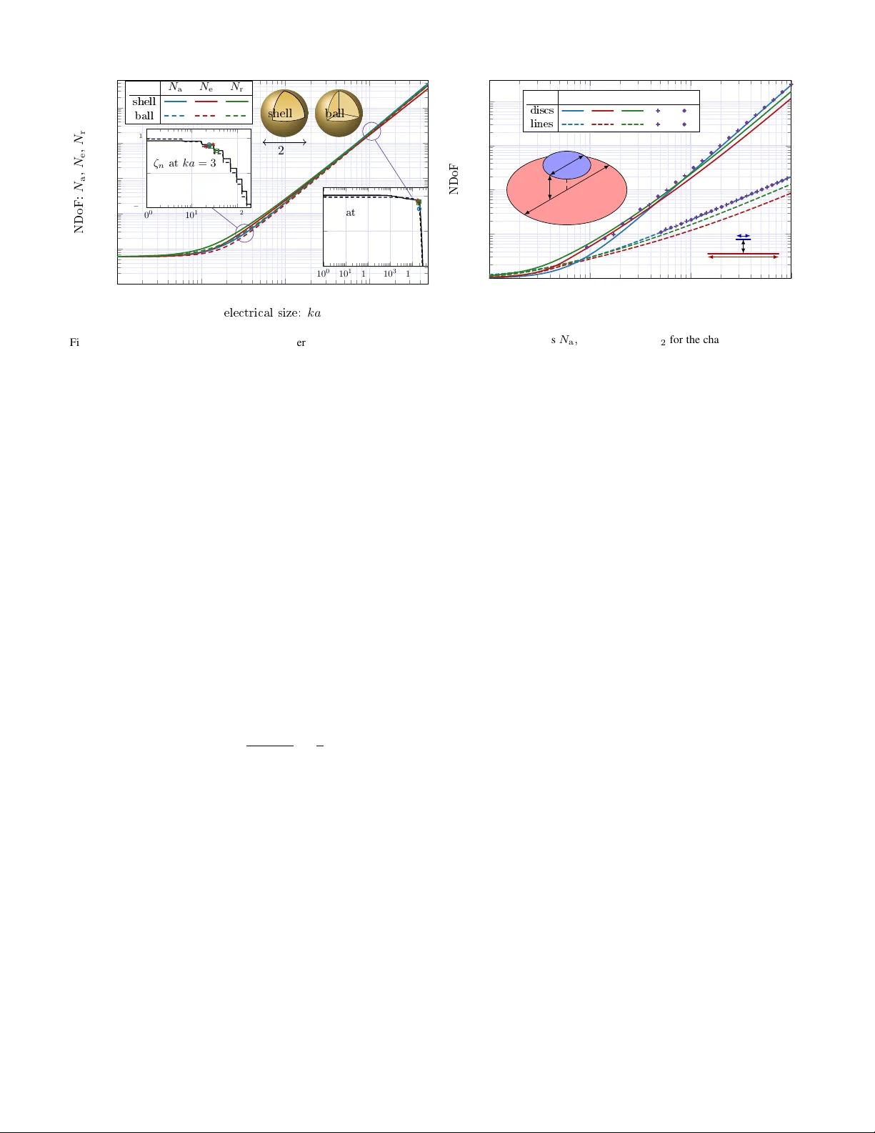
1 Spatial De grees of Freedom and Channel Strength for Antenna Systems Mats Gustafsson and Y ani v Brick Abstract —The number of spatial degrees of freedom (NDoF) and channel strength in antenna systems are examined within a geometric framework. Starting from a corr elation-operator repr esentation of the channel between transmitter and recei ver regions, we analyze the associated eigenspectrum and relate the NDoF to its spectral transition (corner). W e compare the spectrum-based effecti ve NDoF and effective rank metrics, clar - ifying their behavior for both idealized and realistic eigen value distributions. In parallel, we develop geometry-based asymptotic estimates in terms of mutual shadow (view) measures and coupling strength. Specifically , we show that while the projected length or area predicts the number of usable modes in two- and three-dimensional settings, the coupling strength determines the av erage eigen value level. Canonical configurations of parallel lines and regions are used to derive closed-form asymptotic expressions f or the effective NDoF , re vealing significant deviations from the spectral corner in closely spaced configurations. The results illustrate that these ar e physically grounded. The pr oposed theory and techniques are computationally efficient and f orm a toolbox f or estimating the modal richness in near -field channels, with implications for array design, inverse problems, and high- capacity communication systems. I . I N T RO D U C T I O N E LECTR OMA GNETIC channels operating in the near field are attracting increasing interest due to emer ging ap- plications such as high-capacity wireless links, reconfigurable intelligent surfaces, and compact multi-antenna systems [ 1 ]. In these regimes, classical far-field intuition based on angular resolution is insufficient: wa vefront curv ature, strong distance dependence, and geometry-specific coupling significantly in- fluence how many independent communication channels can be supported [ 2 ]–[ 7 ]. A central challenge is, therefore, to quantify the number of degrees of freedom (NDoF) and the associated channel strength in a way that is both physically meaningful and computationally tractable [ 8 ]–[ 21 ]. A common approach characterizes the NDoF through the singular-v alue or eigenspectrum of a channel operator . In MIMO array models, dominant singular values correspond to usable sub-channels, while rapidly decaying values represent weak, noise-sensiti ve modes [ 22 ]. F or continuous electromag- netic systems, this extends naturally to operator formulations based on Green’ s functions, where the eigenspectrum of a correlation operator captures modal coupling between regions. In idealized settings, the NDoF is often associated with a This work was supported in part by the Swedish Research Council SEE- 6GIA and SSF Sabbatical and the Israel Science Foundation (ISF) grant No. 442/22. M. Gustafsson is with Electrical and Information T echnology , Lund Uni- versity , Lund, Sweden, (e-mails: mats.gustafsson@eit.lth.se). Y . Brick is with the School of Electrical and Computer Engineering, Ben-Gurion University of the Negev , Beer-Shev a, Israel 8410501 (e-mail:ybrick@bgu.ac.il). spectral corner separating propagating modes from rapidly decaying reacti ve (ev anescent) contributions [ 8 ]–[ 14 ], [ 16 ], [ 17 ]. Complementary insight is provided by geometry-based ap- proaches, where the NDoF is predicted from quantities such as surface area and propagation directions. This connects to spectral results such as W eyl’ s law [ 23 ], [ 24 ] and sampling- theoretic interpretations of electromagnetic fields [ 13 ]. Recent work indicates that mutual shadow (or view) measures be- tween regions can predict the spectral corner and provide a physical interpretation of near-field spectra [ 17 ], [ 25 ]. While such estimates are intuiti ve and computationally ef ficient, their relationship to spectral metrics such as the effecti ve NDoF [ 26 ], [ 27 ] and effecti ve rank [ 28 ] remains unclear . In this paper , we formulate the electromagnetic channel using correlation operators and compare the spectrum-based effecti v e NDoF and ef fectiv e rank metrics with the geometry- based estimates derived from mutual shadow measures. Their behavior is analyzed for both idealized and realistic eigen- spectra. F or canonical configurations, stationary-phase analysis yields closed-form asymptotic expressions for the ef fectiv e NDoF , rev ealing strong deviations from the spectral corner in closely spaced regimes. These deviations are traced to changes in the propagating eigenspectrum, which transitions from nearly flat for well-separated regions to highly unev en with a few dominant modes at small separations, causing the effecti v e NDoF to vanish as distance decreases. The effecti v e rank is found to be somewhat more robust to variations in the eigenspectrum. The increased spectral variation in config- urations with broad propagation-angle spread is explained by combining observations on the eigenspectrum localization and coupling strength. The main contributions of this work are: • Establish a relationship between the av erage strength of propagating modes and the electromagnetic coupling between regions. • Interpret variations in channel strength in terms of prop- agation directions and geometric visibility . • Pro vide a comparativ e analysis of effecti v e NDoF and effecti v e rank, clarifying their relation to the spectral corner . • Sho w that the effecti ve rank exceeds the effecti ve NDoF and more closely tracks the spectral corner for electrically large structures. • Deri ve asymptotic expressions for the ef fectiv e NDoF in canonical geometries and relate them to mutual shadow–based estimates. The remainder of the paper is organized as follows. Sec- tion II introduces the channel and correlation-operator models, 2 defines spectrum-based NDoF metrics, and presents geometry- based estimates. Section III analyzes canonical configurations and derives asymptotic formulas for parallel lines and planar regions. Section IV discusses the propagating eigenspectra. Conclusions are presented in Sec. V . T echnical deriv ations and details of the Green’ s function are collected in the appendices. I I . D E G R E E S O F F R E E D O M A N D C H A N N E L S T R E N G T H In the analysis of communication between two array anten- nas (e.g., with N T transmitting and N R receiving antennas), the singular values of the channel matrix H ∈ C N R × N T characterize the strength of the av ailable sub-channels [ 22 ]. W eak channels require high signal-to-noise ratios to be useful, and the number of usable sub-channels defines the NDoF [ 13 ]. The squared singular values of H are the eigen values of the N T × N T correlation matrix H H H . For arbitrary array antennas situated in two regions, we construct a communication channel between sources in Ω T and fields in Ω R based on the appropriate (dyadic) Green’ s function G ( r , r ′ ) . Based on this channel, we form an eigen- value problem for the continuous correlation operator R ( r 2 , r 1 ) = Z Ω R G ∗ ( r 2 , r ′ ) · G ( r ′ , r 1 ) dV ′ (1) ov er the current density J ( r ) in Ω T Z Ω T R ( r 2 , r 1 ) · J n ( r 1 ) dV 1 = ζ n J n ( r 2 ) , (2) where the superscript ∗ denotes the complex conjugate. This is a compact operator with a finite number of non-negligible eigen v alues ζ n ≥ ζ 0 > 0 (i.e., abov e a threshold ζ 0 ) [ 8 ], [ 14 ]. The number of significant eigenv alues scales with the areas of Ω T and Ω R for surface domains in R 3 , and with their lengths for line domains in R 2 [ 17 ], [ 25 ]. Note that for surface domains in R 3 and curves in R 2 , the eigen values ζ n hav e a dimension of area. The dyadic Green’ s function notation in ( 1 ) is general and, depending on the formulation, may represent the free-space scalar Green’ s function (for single- or double-layer sources and scalar fields), Green’ s dyadics for current sources and electric fields, or combinations relating electromagnetic fields to physical or equiv alent currents; see App. A . The results presented in this paper are largely independent of the specific Green’ s function. The numerical ev aluations are performed using a discretization of the domains with approximately fiv e points per wa velength, and the resulting eigenspectra exhibit negligible dependence on further dis- cretization refinement, see [ 17 ], [ 25 ] for details. Cases with electromagnetic fields can often be characterized by DoFs of two polarization [ 13 ], [ 14 ]. The NDoF can be reduced for cases with symmetries unless electric and magnetic currents (or single and double-layer sources) are included [ 16 ]. The eigenspectrum typically exhibits a sequence of nearly constant eigenv alues followed by a region of rapidly decaying ones [ 5 ], [ 8 ], [ 13 ], [ 14 ], [ 29 ]–[ 32 ], as illustrated in Fig. 1 . W e refer to the modes preceding the transition as propagating and those follo wing it as reactive. The propagating modes are typically associated with smooth current distributions in the 10 0 10 1 10 2 10 3 10 4 10 − 9 10 − 6 10 − 3 10 0 10 3 r = 8 a r = a a = 10 λ a = 50 λ corner (knee) propagating mo des reactiv e mo des index: n eigen v alue : ζ n r Ω T a Ω R d = a Fig. 1. Eigenspectra for the channels between a transmitting disc region Ω T with radius r ∈ { 1 , 8 } a and receiving disc region Ω R with radius a = { 10 , 50 } λ separated by a distance d = a . The modes up to and after the corner are termed here “propagating” and “reactive”, respectively . region. In contrast, the reacti ve modes are more strongly as- sociated with increasingly oscillatory currents, such as higher- order modes on spherical region [ 33 ], [ 34 ], or currents concen- trated at the edges of the region resembling dif fraction [ 25 ]. The NDoF is associated with this transition corner (or “knee”), where the spectral behavior changes character . In the idealized case, characterized by a uniform plateau fol- lowed by negligible eigenv alues, this corner is well defined and straightforward to identify . In more realistic scenarios, howe v er , the transition may be gradual or in volv e multiple knees, making a unique definition less clear [ 35 ]. As the electrical size increases, the transition becomes more pro- nounced, which moti vates an asymptotic characterization of the NDoF . In this w ork, we therefore focus on electrically lar ge configurations with simple geometries in which a dominant corner is present [ 16 ], [ 17 ], [ 25 ]. This is also similar to the use of asymptotics in W eyl’ s law [ 24 ] and sampling [ 13 ]. As an example, consider the scalar Green’ s function channel between tw o discs with dif ferent radii, r and a with a spacing d = a . The eigenspectrum for this case is shown in Fig. 1 . The eigen v alues for the equal radii case r = a are approximately constant up to the corner , thereafter they decrease rapidly . The corner points are approximately at n ∈ { 380 , 9400 } for the sizes a ∈ { 10 , 50 } λ . This is consistent with the classical λ − 2 scaling with the wavelength λ = 2 π /k of the NDoF [ 14 ], [ 24 ], [ 29 ]. The r = 8 a cases are similar , with corner positions at approximately n ∈ { 1050 , 24800 } . Howe ver , here the spread of the propagating eigen v alues is larger , i.e. , there is approximately a factor of 10 between the first eigen v alues and the eigen v alues just before the corner . Although these cases are numerically tractable, analyti- cal estimates of the eigenspectrum provide insight. Several techniques hav e been dev eloped to quantify the NDoF for these and related situations. These include spectrum-based estimators, such as the effecti ve NDoF [ 26 ], [ 27 ] and effecti ve rank [ 28 ], and geometry-based ones, like those relying on paraxial approximations [ 29 ], [ 36 ] or shadow (projected, vie w) area calculation [ 16 ], [ 17 ], [ 25 ]. 3 A. Spectrum Based Estimates Singular value thresholding is commonly used to regularize ill-posed linear inv erse problems and numerical approxima- tions [ 37 ]. It defines the NDoF as the number of singular values satisfying σ n ≥ ϵσ 1 , i.e., relati ve to the largest singular value. F or the eigen v alues in ( 2 ), ordered by decreasing magnitude, this corresponds to ζ n ≥ ϵ 2 ζ 1 . Alternati vely , normalizing by the least-squares norm yields an NDoF defined by ζ n ≥ ϵ 2 P ζ m . The resulting NDoF depends on the chosen threshold ϵ . Much research has focused on parameter-free techniques to define an NDoF . The effecti ve NDoF [ 26 ], [ 27 ] is commonly used in wireless communications. It is defined by the quotient N e = ( P ζ n ) 2 P ζ 2 n = T r( H H H ) 2 T r( H H HH H H ) = ∥ H ∥ 4 F ∥ H H H ∥ 2 F , (3) here also expressed using the channel matrix H , with either traces or Frobenius norms. The ef fectiv e rank [ 28 ] metric, defined by N r = exp  − X n ( ζ n ln ζ n )  = Y n ζ − ζ n n (4) assuming the normalization P n ζ n = 1 , attempts to estimate the rank of a matrix. This metric is less commonly used than the ef fectiv e NDoF for estimating the NDoF of communication channels. For an ideal channel consisting of N a identical eigen v alues follo wed by negligible eigen v alues, the effecti ve NDoF ( 3 ) and effecti ve rank ( 4 ) coincide with the corner position whereas for more general distributions they typically differ . Jensen’ s inequality shows that N r ≥ N e . The eigen v alue sum, which appears in the normalization of ( 4 ) and in the numerator of ( 3 ), is sometimes referred to as the coupling strength [ 29 ], [ 32 ]. For channels modeled by a scalar Green’ s function, G = exp( − j k r ) / (4 πr ) with r = | r | , it is given by X n ζ n = ∥ H ∥ 2 F = Z Ω T Z Ω R | G ( r − r ′ ) | 2 dS dS ′ . (5) This term is frequency independent and easily ev aluated nu- merically for arbitrarily shaped regions. For channels modeled via Green’ s dyadics, it exhibits weak frequency dependence but stabilizes at high frequencies. For the 2D Green’ s function, the Frobenius norm in the expression is proportional to the wa velength in the high-frequency limit, see App. A . The corner position N c can also be determined by inspection or image processing techniques. F or the simple cases in this paper with one dominant corner , the position can e.g. , be estimated by the minimal least squares fit of the spectrum in a logarithmic scale (ln n, ln ζ n ) to two lines. B. Geometry-Based Estimates Geometry-based approaches use simple properties of the regions, such as their surf ace area or shadow (projected) area, to estimate the NDoF . This resembles the fundamental results on the Laplacian eigen v alue distrib ution by W eyl [ 23 ], [ 24 ] and sampling theorems by Whittaker , Nyquist, and Shannon [ 13 ]. These results are asymptotic, e.g . , in R 1 stating that the number of modes [ 23 ], [ 24 ] on a line with length ℓ is 2 ℓ/λ , which corresponds to λ/ 2 sampling [ 13 ]. The total mutual shadow (projected or view) area A TR (or length L TR ) between a transmitter and receiv er measured in wa velengths determines the asymptotic NDoF [ 16 ], [ 17 ] N a = ( L TR /λ in R 2 A TR /λ 2 in R 3 (6) per polarization DoF . The mutual shado w area can be ev alu- ated analytically for canonical geometries and numerically for arbitrary-shaped structures [ 17 ]. For a simple shape in which ev ery point of Ω R is visible from Ω T , the total mutual shadow (view) area is [ 17 ], [ 25 ] A TR = Z Ω T Z Ω R | ˆ n ′ · R | | ˆ n · R | | R | 4 dS ′ dS , (7) with R = r − r ′ denoting a vector connecting points in Ω T and Ω R and ˆ n the unit normal of the surface. In 2D, it reduces to the total mutual shadow length L TR = Z Ω T Z Ω R | ˆ n ′ · R | | ˆ n · R | | R | 3 d l ′ d l, (8) see [ 17 ] for more general configurations. The total mutual shadow (projected) area and length simplify to π A and 2 L for a con ve x transmitter region surrounded by a receiv er region [ 16 ], with surface area A and circumference L , in agreement with W e yl’ s law and sampling theory [ 16 ]. Similar expressions to ( 7 ) and ( 8 ) have been extensiv ely used in thermal radiative heat transfer [ 38 ], [ 39 ], where they are related to radiation view factors. Many analytical ev aluations for simple configurations are presented in [ 38 ], [ 39 ]. For example, the two discs in Fig. 1 have a total mutual shadow (view) area A TR = π 2 2  ∆ − p ∆ 2 − 4 a 2 r 2  (9) with ∆ = a 2 + r 2 + d 2 , giving N a ∈ { 377 , 9425 } for the r = a case and N a ∈ { 972 , 24289 } for the r = 8 a case using ( 6 ). These are in good agreement with the knee positions seen in the numerical data in Fig. 1 . For well-separated small regions, the mutual shado w area ( 7 ) simplifies to A P = 1 d 2 Z Ω T | ˆ n · ˆ R | dS Z Ω R | ˆ n · ˆ R | dS , (10) with the distance d and direction ˆ R = R /R . F or perpendicular surfaces, this expression reduces to the well-known paraxial approximation [ 29 ] A P = A T A R /d 2 , where A X denotes the area of Ω X for X ∈ { T , R } . Combining the coupling strength ( 5 ) with the mutual shadow area ( 7 ) sho ws that the a verage le v el of the propagating part of the spectrum per squared wa velength is approximately (4 π ) 2 P ζ n λ 2 N a = Z Ω T Z Ω R 1 R p dS dS ′ Z Ω T Z Ω R | ˆ n ′ · ˆ R | | ˆ n · ˆ R | R p dS dS ′ ≥ 1 , (11) 4 10 − 1 10 0 10 1 10 2 10 0 10 1 10 2 10 3 10 4 10 5 electrical size: k a NDoF: N a , N e , N r N a N e N r shell ball shell 2 a ball 10 0 10 1 10 2 10 − 9 10 − 5 10 − 1 ζ n at k a = 3 10 0 10 1 10 2 10 3 10 4 10 − 12 10 − 8 10 − 4 ζ n at ka = 100 Fig. 2. NDoF estimates N a , N e , and N r for spherical shells and balls versus the electrical size k a . Insets depict the corresponding eigen values ζ n at k a ∈ { 3 , 100 } with markers indicating the estimated NDoF . assuming a scalar Green’ s function ( 28 ) and p = 2 . This purely geometrical quantity reduces to unity in the paraxial limit for perpendicular surfaces. The corresponding av erage in 2D is obtained by setting p = 1 in ( 11 ), where the high-frequency approximation of the Green’ s function ( 29 ) is used. The identity ( 11 ) is here referred to as the asymptotic a ver- age channel strength. Note that, for arbitrary-shaped regions, the inte gration in the numerator e xtends o ver the entire re gions, whereas that in the denominator is ef fectiv ely restricted to their mutually observ able parts [ 17 ], which increases the resulting av erage channel strength. The factor λ 2 in ( 11 ) compensates for the dimensionality of ζ n (area) in ( 2 ). For other con- figurations, such as lines or volumes in 3D, corresponding weightings can be obtained straightforwardly by combining the coupling strength with the appropriate shadow measure. The asymptotic average channel strength ( 11 ) also suggests a simple threshold-based NDoF estimate N 1 / 2 defined by the number of normalized eigenv alues greater than 1 / 2 , i.e. , N 1 / 2 = card  (4 π ) 2 ζ n λ 2 ≥ 1 2  . (12) C. Comparison The NDoF metrics N e in ( 3 ) and N r in ( 4 ) are first e v aluated for spherical shell and solid ball transmitter domains and receiv ers on the entire far-field sphere. The sources are electric and magnetic currents, for electrical sizes k a ∈ [1 , 500] , as depicted in Fig. 2 . For both geometries, both spectral estimates agree well, con ver ge to 6 for k a → 0 , and scale with k 2 for lar ge k a . Small differences are mainly observed around k a ≈ 1 , but also a slight difference in the slope for large k a can be seen. The comparison also includes a modified NDoF estimate based on the shadow area ( 6 ) with a lo w-frequency asymptotic correction [ 17 ], i.e. , N a → N a + 6 . The NDoF in Fig. 2 also agree with the classical approach based on the number of propagating spherical modes [ 33 ], [ 40 ], [ 41 ] N = 2 L ( L + 2) = 2 L 2 + 4 L (13) 10 − 1 10 0 10 1 10 2 10 0 10 1 10 2 10 3 10 4 ℓ/λ NDoF N a N e N r N c N 1 / 2 discs lines ℓ 10 ℓ ℓ 10 ℓ Ω R ℓ Ω T ℓ Fig. 3. NDoF estimates N a , N e , N r , N c , N 1 / 2 for the channels between two discs (solid curves) in R 3 and two lines (dashed curves) in R 2 . for spherical harmonic order L , using the common estimate L = ka ≥ 1 for the onset of modes. Here, we also note that N ≈ 2 N a = 2 π A/λ 2 as λ → 0 in agreement with ( 6 ) and ( 7 ). The eigen v alue curves ζ n for k a ∈ { 3 , 100 } are depicted in the insets in logarithmic scale. The corners are observed around 2 N a = 2( ka ) 2 = { 18 , 2000 } for the two cases, in agreement with ( 13 ). The corner becomes increasingly pronounced as k a increases. Until the corner is approached, the spectrum is quite uniform in magnitude. As a second example, the various NDoF estimates for chan- nels between two disc domains in R 3 and two line domains in R 2 are shown in Fig. 3 (see inset for geometry details). For small electrical sizes ℓ/λ , the NDoFs estimates are low and differ from one another by ± 1 roughly . In this regime, N a is modified by including the low-frequenc y contribution [ 17 ], i.e. , N a → N a + 1 , and the corner NDoF N c and threshold NDoF N 1 / 2 are excluded from the study due to the inherent difficulty of defining a distinct spectral corner when only a few modes are present. For electrically larger sizes, the NDoF estimates exhibit ap- proximately straight line trends in the log-log plot, indicating a po wer law behavior N x ≈ α x /λ p for N x ≫ 1 (14) with p = 2 for the discs and p = 1 for the lines. The dominant term α x is determined by the short wa velength limit of the NDoF . The NDoF estimates in Fig. 3 diver ges and are ordered as N e < N r < N a ≈ N c ≈ N 1 / 2 . The inequality N e < N r holds in general; to further examine the relationship among the remaining estimates, the offsets α x between the curves should be analyzed. As part of the proposed analysis, in the next section, the small-wa velength asymptotic behavior of N e is examined. I I I . A S Y M P T OT I C E V A L UAT I O N O F N e The ef fectiv e NDoF , N e in ( 3 ), is typically e valuated numerically , as illustrated in Fig. 2 and Fig. 3 . While the results in Fig. 2 show good agreement, those in Fig. 3 e xhibit more significant deviations. As shown here, the discrepancies 5 increase for closely spaced configurations. These observations, which rely on numerical experiments, are supported by an asymptotic analysis of N e in the electrically large regime, which enables a direct comparison between the N e and N a metrics. In this asymptotic analysis, N e is e v aluated by reformulating the terms in ( 3 ) as multidimensional integrals and subsequently deriving their leading-order beha vior . The denominator in ( 3 ), i.e. , P ζ 2 n , is ∥ H H H ∥ 2 F = Z Z Z Z G ∗ 1 , 1 ′ G 2 , 1 ′ G ∗ 2 , 2 ′ G 1 , 2 ′ dS 2 dS ′ 2 dS 1 dS ′ 1 (15) with the short-hand notation G m,n ′ = G ( r m , r ′ n ) . This mul- tidimensional oscillatory integral (defined ov er R 4 for lines, R 8 for surfaces, and R 12 for volumes) is not well suited for direct numerical ev aluation. Howe ver , it is amenable to asymptotic analysis via stationary phase methods [ 42 ], which yield analytic expressions in the short-wa velength limit. The product of the Green’ s functions ( 15 ) can be written as exp( − j k ϕ ) h , where the phase ϕ is ϕ = | r 1 − r ′ 1 | − | r 2 − r ′ 1 | + | r 2 − r ′ 2 | − | r 1 − r ′ 2 | (16) and h contains a product of 1 / | r 1 − r ′ 1 | type terms. Assuming a single stationary point at r 0 giv es [ 42 ] Z f ( r )e j kϕ ( r ) dV = λ n/ 2 f ( r 0 )e j kϕ ( r 0 )+j π 4 sgn( H ϕ ) | det( H ϕ ) | 1 / 2 + o ( λ n/ 2 ) (17) as λ → 0 , where H ϕ denotes the Hessian at r 0 . The stationary points with respect to variations over r 2 , r ′ 2 are giv en by the zeros of ∇ 2 ϕ and ∇ ′ 2 ϕ . W e apply the technique to the canonical cases of two parallel lines and two parallel plates. A. T wo parallel lines The asymptotic ef fectiv e NDoF for short wa velengths is first determined for two parallel lines in 3D with length ℓ 1 and ℓ 2 separated by a distance d , as shown in the inset of Fig. 4 . The stationary phase approximation of the effecti ve NDoF ( 3 ) deriv ed in App. B is N 0 e = ℓ 2 λ  ln(1 + β 2 ) − 2 β atan( β )  2 β 2 asinh( β ) − β p β 2 + 1 + β (18) as λ → 0 with β = ℓ/d . This asymptotic expression for the effecti v e NDoF is illustrated in Fig. 4 (dashed red line labeled “3D”). For large separation distances β → 0 , the limit N 0 e → ℓ 2 / ( dλ ) coincides with the paraxial limit. For short distances, the limit is N 0 e ≈ ℓ 2 λ 2 π ln(2 β ) → 0 as β → ∞ , (19) i.e. , it vanishes logarithmically as d → 0 , as suggested by the slow decay of the corresponding curve in Fig. 4 . The NDoF based on the total mutual shadow length ( 8 ) (blue line in Fig. 4 ) is given by N a = L TR λ = 2 ℓ λ p 1 + β 2 − 1 β ≥ N 0 e . (20) 10 − 2 10 − 1 10 0 10 1 0 0 . 5 1 1 . 5 2 2 . 5 L TR /ℓ corner N r λ ℓ N r λ ℓ N e λ ℓ N e λ ℓ 3D 2D par-axial distance: d/ℓ NDoF p er w a v elength ℓ ℓ d Fig. 4. NDoFs per wavelength for the channel between two lines with length ℓ and separation distance d . The shadow-length estimate ( 20 ) is shown by the solid curve, the asymptotic effectiv e NDoF in 3D and 2D from ( 18 ) and ( 21 ), respectiv ely , by dashed curves, and the paraxial approximation by a dash- dotted curve. Analytical results are compared with numerical estimates of the effecti ve NDoF ( 3 ), effectiv e rank ( 4 ), and corner position for wavelengths λ ∈ { 1 , 2 , 4 } 0 . 01 ℓ , indicated by small to large markers. It is greater than or equal to the effecti ve NDoF ( 18 ) for sufficiently short w av elengths and also approaches the paraxial approximation for large separation distances and 2 ℓ/λ as d → 0 in agreement with W eyl’ s law [ 17 ]. The closed form shado w area estimate and asymptotic effecti v e NDoF are compared with numerical ev aluation of the various NDoF estimates, for a model of the channel between the lines obtained by their sampling with five points per wa velength, for λ ∈ { 1 , 2 , 4 } 0 . 01 ℓ , as shown in Fig. 4 (corresponding color markers of sizes decreasing with λ ). The numerically e valuated N e shows increasingly good agreement with the analytical result as λ decreases. Likewise, the numer - ically estimated eigen value corner points agree well with the mutual shado w length ( 20 ). The limits di ver ge as d/ℓ → 0 , where it is seen that N e λ/ℓ decreases for small d/ℓ and falls below the mutual shadow length L TR . This decrease in effecti ve NDoF at small separation distances is somewhat counterintuitiv e. This can be explained by the behavior of the eigen v alue spectrum as a function of d , as is shown next. The eigenspectra for the channels between the two lines in 3D at λ = 10 − 3 ℓ are sho wn in Fig. 5 , with the normalized index axis n/ N a . For all d/ℓ v alues, a clear corner (knee) ap- pears around n = N a , beyond ( n > N a ) which the eigen values are negligible, for all separation distances. Markers indicate the effecti v e NDoF ( 3 ) and rank ( 4 ) estimators. In the range n < N a , the eigen values remain relati vely constant only for relativ ely lar ge separation distances. For these cases, the corner is predicted correctly . For shorter distances, where the NDoF is underestimated (as seen also in Fig. 4 ), a pronounced variation is observed between the leading eigen v alues ( n ≈ 1 ) and the subsequent ones. Here, it is worth noting that the normal- ization ( 5 ) implies a unit area under each curve in Fig. 5 . V ariations in eigenv alue distribution do manifest, howe ver , in the denominator of ( 3 ), due to the squaring of the eigenv alues. The greater the variation, for the same corner value, the lo wer the v alue predicted by ( 3 ). 6 0 0 . 2 0 . 4 0 . 6 0 . 8 1 0 1 2 3 n/ N a N a ζ n / P ζ n d/ℓ 0 . 1 0 . 2 0 . 4 0 . 8 1 . 6 3 . 2 ζ n N e N r N a 1810 1640 1354 961 574 305 Fig. 5. Normalized eigenspectra for two lines with length ℓ separated a distance d at wa velength λ/ℓ = 10 − 3 , cf. , inset in Fig. 4 . NDoFs N e and N r are indicated by the markers and N a is ev aluated from ( 20 ). Similarly , a high-frequency asymptotic expression for the effecti v e NDoF can be derived for parallel lines in R 2 . The deriv ation of such an expression in App. B , for λ → 0 , results in N 0 e = ℓ λ 4 β (asinh β − p 1 + β − 2 + β − 1 ) 2 2 3 + β asinh( β ) − p 1 + β 2 + 1 3 (1 + β 2 ) 3 / 2 . (21) The resulting effecti v e NDoF per wav elength N 0 e λ/ℓ is shown in Fig. 4 (dashed yellow line, labeled “2D”). These results agree with the 3D ( 18 ), the mutual shado w length ( 20 ), and paraxial approximation for larger separation distances, i.e. , d > 2 ℓ . For shorter distances, they are the lowest of all estimates and grossly underestimate the corner position. The numerically ev aluated N e values using ( 3 ) approach N 0 e as the wa velength decreases. B. T wo parallel planar r e gions The asymptotic analysis for the case of parallel lines in Sec. III-A readily extends to parallel planar regions, as sho wn in App. C . The dominant term in the asymptotic expansion of P ζ 2 n is ∥ H H H ∥ 2 F ≈ λ 2 (4 π ) 4 Z Z R 6 d 2 R 6 dS dS ′ = λ 2 A T A R (4 π ) 4 d 2 . (22) The coupling strength normalization term is ∥ H ∥ 2 F = 1 (4 π ) 2 Z Z dS dS ′ ( x − x ′ ) 2 + ( y − y ′ ) 2 + d 2 . (23) For rectangular regions, using ( 35 ), it is reduced to a 2D integral. Substituting these expressions into ( 3 ) yields the dominant term of the effecti ve NDoF N 0 e = ∥ H ∥ 4 F d 2 (4 π ) 4 λ 2 A T A R ≤ A TR λ 2 , (24) where the inequality follo ws from applying the Cauchy–Schwarz inequality to the coupling strength ( 23 ), such that ∥ H ∥ 4 F ≤ A T A R (4 π ) 4 Z Z 1 R 4 dS dS ′ = A T A R (4 π ) 4 A TR d 2 . (25) 0 . 01 0 . 1 1 10 0 1 2 3 A TR / A corners N 0 e λ 2 / A par-axial A d 2 N r λ 2 / A distance: d/a NDoF p er w a v elength 2 , N λ 2 / A a Ω T a Ω R A = π a 2 d λ/a N c N e N r 0.04 0.02 0.01 Fig. 6. Normalized NDoF for two discs with radius a separated a distance d . Numerical results using wav elengths λ/a ∈ { 0 . 04 , 0 . 02 , 0 . 01 } are indicated by the markers, with squares indicating corner positions N c , circles N e ( 3 ), and asterisks N r ( 4 ). The numerical results are compared with analytical expressions for shadow area ( 9 ) (solid lines), stationary phase asymptotic N e in ( 24 ) (dashed), and the paraxial approximation (dashed dotted). Hence, the effecti ve NDoF N e is always bounded by the normalized shadow area N a for sufficiently short wav elengths. Equality is achieved when the variation of the R − 4 term is negligible, i.e. , when the distance between the regions is much larger than their characteristic size, as in the paraxial approximation ( 10 ). The asymptotic expression can be calculated for the case of parallel identical discs presented in Fig. 6 . In cylindrical coordinates, the coupling strength ( 23 ) reduces to ∥ H ∥ 2 F = Z r 0 Z a 0 ρρ ′ d ρ d ρ ′ p ( ρ + ρ ′ ) 2 + d 2 p ( ρ − ρ ′ ) 2 + d 2 , (26) which can be readily ev aluated numerically . The dominant term of the ef fecti ve NDoF , N 0 e , computed using ( 24 ) and ( 26 ), is shown by the dashed curve in Fig. 6 . T o facilitate the comparison, the values are normalized by λ 2 and the disc area A = π a 2 . The quantity N 0 e is small for both short and large separations, with a maximum at intermediate distances. For large separations, d > a , it agrees well with the total mutual shadow area ( 9 ). For d > 3 a , it also agrees with the paraxial approximation [ 29 ], [ 36 ]. The significant deviation observed for d < a is consistent with the Cauchy–Schwarz inequality ( 25 ), as the R − 2 term varies considerably in this regime. The numerical v alues of N e , computed for λ ∈ { 0 . 04 , 0 . 02 , 0 . 01 } a , approach N 0 e as the wa velength decreases, similarly to the case of parallel lines in Fig. 4 . Also presented are the numerical e valuations of N r , and corner position, which too coincide for larger separations. The corner positions show excellent agreement with the shadow area-based estimate in the entire range. The corresponding eigenspectra for the wa velength λ = 0 . 01 a and distances d = { 0 . 1 , 0 . 2 , 0 . 4 , 0 . 8 , 1 . 6 , 3 . 2 } a are depicted in Fig. 7 . The computed effecti ve NDoF N e and effecti v e rank N r are indicated by markers. Here too, it is observed that N e ≈ N r ≈ N a for the larger separation distances, where the propagating eigenspectrum is relati vely 7 0 0 . 2 0 . 4 0 . 6 0 . 8 1 10 − 1 10 0 10 1 n/ N a ζ n (4 π /λ ) 2 a Ω T a Ω R A = π a 2 d d/a 0 . 1 0 . 2 0 . 4 0 . 8 1 . 6 3 . 2 ζ n N e N r N a 89308 80832 66331 45240 22799 8118 Fig. 7. Eigenspectrum for two discs with radius a separated a distance d at wav elength λ = 10 − 2 a normalized according to ( 11 ). NDoFs N e and N r are indicated by the markers and N a is ev aluated from ( 6 ) and ( 9 ), cf. , Fig. 6 . flat. The three predictors dif fer greatly for shorter distances, where the variation in the propagating eigenspectrum is larger . T o conclude, for both the lines and flat surface in 3D, as well as in 2D, the deviation of N e from N a can be predicted analytically for short wa velengths and is indicative of the variation in the propagation spectrum eigenv alues. I V . P R O P AG A T I N G E I G E N S P E C T R U M D I S T R I B U T I O N Insight into the behavior of the propagating eigenspectrum can be obtained from its av erage value ( 11 ). By bounding the integrand in the denominator using its minimal and maximal values, we obtain 1 max ˆ R | ˆ R · ˆ n T | | ˆ R · ˆ n R | ≤ (4 π ) 2 P ζ n λ 2 N a ≤ 1 min ˆ R | ˆ R · ˆ n T | | ˆ R · ˆ n R | , (27) where ˆ R denotes the propagation direction between points in Ω T and Ω R , and ˆ n X is the unit normal of Ω X . These bounds show that the av erage lev el of the propagating eigenspectrum is governed by the incidence angles between the propagation directions and the surface normals at the transmitter and receiv er . Regions for which | ˆ R · ˆ n X | is small can therefore contribute to larger eigenv alues. Consequently , the av erage lev el increases with angular misalignment from the broadside direction, i.e. , endfire configurations can yield higher eigen- values than broadside configurations. In this context, it is worth noting that the case in Fig. 2 , in volving a spherical source and a far-field observation sphere, is highly symmetric and provides an extreme example of directional uniformity of all directional beams and observation sectors and, thus, exhibits a rather flat spectrum. Similarly , the much-studied paraxial cases with well-separated parallel regions have low angular di versity and a relatively flat spec- trum. T o further understand the v ariation within the propagating eigenspectrum, we assume that the interaction between the 0 0 . 2 0 . 4 0 . 6 0 . 8 1 10 − 1 10 0 10 1 b n/ N a ζ n (4 π /λ ) 2 ℓ 10 ℓ ℓ a) b) Ω R Ω T d) Ω Rc Ω Rs c) ζ n N e N r a) b) c) d) Fig. 8. Normalized eigenspectrum for four configurations (a) to (d) with identical N a ev aluated for λ = 0 . 002 ℓ . Effecti ve NDoF N e and rank NDoF N r are indicated by markers. Case (d) is ev aluated by splitting Ω R into two separate regions Ω Rc and Ω Rs and merging the eigen values in postprocessing. regions can be approximately localized in the electrically large limit, i.e. , that the overall interaction can be decomposed into contributions from pairs of subregions. This type of asymp- totic localization underlies, for example, certain deriv ations of W eyl’ s law . In [ 25 ], the propagating spectrum (up to the corner N a ) is shown to be associated with directional, beam- producing aperture singular vectors that exhibit localized fields at the observation region. W ith this in mind, the propagating eigenspectrum is in- vestigated by comparing four configurations with identical mutual shadow area values, as illustrated in Fig. 8 , with the normalized axis n/ N a . The two parallel lines in (a) consist of a transmitter of length ℓ and a receiv er of length 10 ℓ , separated by a distance ℓ . The eigenspectrum for λ = 0 . 02 ℓ resembles the equal-line case in Fig. 5 , with a few initially v ery strong eigenv alues followed by approximately equal-strength eigen v alues up to the NDoF n ≈ N a . The effecti ve NDoF N e ≈ 0 . 4 N a and ef fectiv e rank N r ≈ 0 . 66 N a , as indicated by markers in Fig. 8 are positioned in the relativ ely flat part of the eigenspectrum, relativ ely far from the corner around n = N a . Comparing the numerically computed eigenv alues with the estimate in ( 27 ), the most oblique propagation direction, occurring between the edges of the regions, yields an upper bound of 31 . 25 for the normalized eigen v alues, which is in good agreement with a normalized numerical value for ζ 1 that is roughly 25 in Fig. 8 . Replacing the recei ving line by a circular arc, as in Fig. 8 b, while preserving the value for the mutual shadow area, pro- duces a significantly flatter eigenspectrum before the corner at n ≈ N a . The arc geometry yields approximately equal distances between the transmitter and the different parts of the receiv er and propagation directions approximately normal to Ω R for the localized beams produced by the transmitter that illuminate them, i.e. , ˆ R · ˆ n R ≈ 1 in ( 27 ). The angular variation at Ω T is the same as in case (a) leading to a bound of approximately 5 . 6 , which agrees well with the largest eigen v alue ζ 1 of around 5 . This reduces spectral v ariation across dif ferent beam-producing modes and yields a more 8 balanced distribution. Consequently , both the ef fectiv e NDoF N e ≈ 0 . 84 N a and the effecti ve rank N r ≈ 0 . 93 N a mov e closer to the asymptotic value N a . The hybrid geometry in Fig. 8 c exhibits mixed spectral behavior , characterized by a small set of dominant eigenv alues followed by a broad, nearly flat region. Specifically , the spectrum initially resembles configuration (a) for n < 0 . 07 N a , with a few strong modes, and transitions to a flat distribution similar to configurations (b) and (c) for n > 0 . 07 N a . This transition is consistent with a partitioning of the shadow length between the flat and curved segments, i.e. , L TR /ℓ ≈ 0 . 13 + 1 . 83 , where the flat portion accounts for approximately 7% of the total shadow length. These observ ations also support the approximate localization perspectiv e: different parts of the interacting re gions contribute distinct propagating spectral bands that combine additi vely for the dominant propagating modes. The localization observ ation is further supported by the spectrum for the configuration in Fig. 8 d. There, the receiver region Ω R is partitioned into flat shoulders and arc subregions, Ω Rs and Ω Rc . The channels from Ω T to each subregion are formed and their eigen values are computed separately prior to their sorted merging. The combined spectrum is shown in yellow and red cross markers for eigen values associated with Ω Rs and Ω Rc , respectiv ely . These eigen values follow closely those of case (c), with only minor differences, pri- marily around the transition region near n ≈ 0 . 07 N a . The results in Fig. 8 further indicate that the strongest eigenv alues are primarily associated with the shoulders of the receiving region Ω R , where propagation angles are largest, rather than with the central region characterized by shorter distances. Consequently , the NDoF predicted from the shado w area N a and those inferred from spectral measures such as N e and N r may dif fer in configurations with significant v ariation in the propagation angle of the interaction. The comparison also indicates that large-angle interactions primarily determine the largest eigenv alues, whereas the mutual shadow governs the asymptotic position of the corner . These observ ations are consistent with the spectral analysis in [ 25 ]. The analysis links the largest singular v alues of the to the singular vectors that radiate the beams of the greatest oblique angle seen by the observer . For observers significantly wider than the source, as in Fig. 8 a, the beams become localized at regions of the observer and the v ariation in the singular v alues increases. The last set of examples examines the propagating eigen- spectrum for six different configurations (see Fig. 9 insets) with similar mutual shadow lengths. Here, the domains are relativ ely more distant then in the previous example. In Fig. 9 , star and circle markers indicate N e and N r . Case (b) with two well-separated parallel lines shows a flat propagating eigen- spectrum, as in Fig. 5 . The normalized amplitude is unity in the scaling from ( 11 ) as motiv ated by the propagation directions normal to the Ω T and Ω R regions ( 27 ). The propagating eigenspectra for cases (a) and (c) are also relatively flat. Their av erage amplitude, howe ver , is higher because of the oblique directions, following ( 27 ). All these cases hav e NDoFs N e and N r close to the corner around n = N a . 0 0 . 2 0 . 4 0 . 6 0 . 8 1 10 − 1 10 0 10 1 n/ N a ζ n (4 π /λ ) 2 b) c) a) d) f ) e) Fig. 9. Eigenspectrum for six different setups with similar N a ≈ 138 ev aluated for λ = 0 . 001 ℓ . The av erage distances R 0 are similar for (bdef) and slightly larger for (ac). Effectiv e NDoF N e and effectiv e rank N r are indicated by circle and star markers, respectively . Case (d), where the domains are closer together and ex- hibit greater variation in the range of observ ation angles and distances, shows a larger v ariation within the eigen values and also a larger av erage. The resulting NDoFs N e and N r are now clearly belo w the corner position. Cases (e) and (f) hav e recei ving regions consisting of a square in (f) and three inscribed squares in case (e). They hav e the same visible part as case (b), but extend farther behind the line in (b). Therefore, the shado w area remains unchanged, while the coupling strength increases due to the larger total support, b ut with no increase in the angular div ersity . Howe ver , the NDoFs N e and N r are well below the corner , with e.g . , N e ≈ { 0 . 3 , 0 . 5 } N a . The examples highlight a trade-off between shado w area, which gov erns the corner position, and region size and sep- aration, which influence modal strength. In particular , larger visible re gions increase the number of a vailable propagating modes. Larger regions (even if not fully visible to one an- other) increase the av erage modal strength. Increased distance reduces the number of propagating modes and the av erage modal strength. V . C O N C L U S I O N S W e presented a unified framework for quantifying spa- tial degrees of freedom and channel strength in radiativ e electromagnetic systems by combining operator -spectrum and geometry-based analyses. The results indicate that two quan- tities, mutual shado w (view) area and coupling strength, cap- ture the main characteristics of the propagating eigenv alue spectrum. Specifically , the mutual shado w area determines the spectral-corner location, while coupling strength governs the av erage lev el of propagating eigen v alues and thus the ov erall channel strength. Using a correlation-operator formulation, we compared spectrum-based NDoF metrics, namely effecti v e NDoF and effecti v e rank, with geometry-based estimates derived from mutual shadow area. The analysis shows that these metrics 9 are consistent for simple configurations under paraxial con- ditions. For more general geometries, effecti ve rank typically exceeds effecti ve NDoF , while both remain below shadow- based NDoF estimates that track the spectral corner more closely . Asymptotic e valuations for canonical parallel-line and parallel-region configurations in two and three dimensions support these findings and clarify when paraxial interpretations remain accurate. Differences between spectral and geometric metrics are pri- marily explained by variability within the propagating eigen- value spectrum. Configurations with large angular spreads or complex geometries exhibit greater modal variability , which causes effecti ve NDoF and effecti v e rank to underestimate the corner location. Overall, the proposed framework provides physically in- terpretable and computationally ef ficient tools for estimating modal richness and coupling strength in near-field electro- magnetic channels. These results are relev ant to antenna-array design, electromagnetic in verse problems, integral equations, and high-capacity communication systems, where geometry and propagation distance critically influence performance. A P P E N D I X A G R E E N ’ S F U N C T I O N S This appendix summarizes the Green’ s functions used in the operator formulation in Section II and in the asymptotic deriv ations. The scalar Green’ s function in R 3 is G 3 = exp( − j k r ) 4 π r , (28) and the Green’ s dyadic is G = ( 1 + k − 2 ∇∇ ) G 3 . In R 2 , the corresponding scalar Green’ s function is G 2 = j 4 H (2) 0 ( k r ) ≈ 1 4 r 2 j π kr e − j kr = 1 4 π s λ j r e − j kr (29) as k r → ∞ , where H (2) 0 denotes a Hankel function. A P P E N D I X B D E R I V AT I O N F O R T W O PA R A L L E L L I N E S This appendix deriv es the stationary-phase approximation for two parallel lines used in Section IV . Consider two parallel lines with length ℓ 1 and ℓ 2 separated by a distance d . The stationary points are given by the zeros of ∂ ϕ ∂ x 2 = x 2 − x ′ 1 p ( x 2 − x ′ 1 ) 2 + d 2 − x 2 − x ′ 2 p ( x 2 − x ′ 2 ) 2 + d 2 (30) and similar for ∂ ϕ ∂ x ′ 2 . This system can be solved by squaring the terms ( x 2 − x ′ 1 ) 2 (( x 2 − x ′ 2 ) 2 + d 2 ) = ( x 2 − x ′ 2 ) 2 (( x 2 − x ′ 1 ) 2 + d 2 ) (31) which simplifies to ( x 2 − x ′ 1 ) 2 = ( x 2 − x ′ 2 ) 2 and inserting into ( 30 ) x 2 − x ′ 1 = x 2 − x ′ 2 and x ′ 1 = x ′ 2 . Similarly , from ∂ ϕ ∂ x ′ 2 we also find x 1 = x 2 . The Hessian in ( 17 ) at the stationary point follows from ∂ 2 ϕ ∂ x 2 2 = 0 and the mixed term ∂ 2 ϕ ∂ x 2 ∂ x ′ 2 = R 2 − ( x 1 − x ′ 1 ) 2 R 3 = d 2 R 3 . (32) Thus, the Hessian is H ϕ = d 2 R 3  0 1 1 0  with | det( H ϕ ) | 1 / 2 = d 2 R 3 (33) A. Lines in 3D The phase at the stationary point is ϕ = 0 giving the stationary phase integral ( 17 ) ( β = ℓ/d ) λ Z Z R 3 d 2 R 4 d l 1 d l ′ 1 = λ d 2 Z Z 1 p ( x 1 − x ′ 1 ) 2 + d 2 d l 1 d l ′ 1 = 2 λ ℓ ( β 2 asinh( β ) − β p β 2 + 1 + β ) (34) The coupling strength from ( 5 ) gives ∥ H ∥ 2 F = 1 (4 π ) 2 Z Z 1 ( x 1 − x ′ 1 ) 2 + d 2 d l 1 d l ′ 1 = 2 β atan( β ) − ln(1 + β 2 ) (4 π ) 2 (35) which yields the dominant asymptotic term in ( 18 ). B. Lines in 2D The Green’ s function in 2D ( 29 ) has the same asymptotic phase as in 3D as kr → ∞ and only dif fers by the slower amplitude decay . This gives the same stationary points as for the 3D Green’ s function in ( 28 ) and the same Hessian ( 33 ). The stationary phase integral ( β = ℓ/d ) λ Z Z R 3 d 2 R 2 d l 1 d l ′ 1 = λ d 2 Z Z q ( x 1 − x ′ 1 ) 2 + d 2 d l 1 d l ′ 1 = 2 3 + β asinh( β ) − p 1 + β 2 + 1 3 (1 + β 2 ) 3 / 2 . (36) W ith normalization from the coupling strength ( 5 ), ∥ H ∥ 2 F = Z Z 1 (( x 1 − x ′ 1 ) 2 + d 2 ) 1 / 2 d ℓ 1 d l ′ 1 = asinh β − p 1 + β − 2 + β − 1 (37) giving the asymptotic ratio entering the effecti ve-NDoF ex- pression ( 21 ) and therefore the same linear-in- ℓ/λ scaling with geometry factor β as in the 3D line case. A P P E N D I X C D E R I V AT I O N F O R T W O PA R A L L E L R E G I O N S This appendix outlines the stationary-phase Hessian struc- ture for two parallel regions used in Section VI. The stationary points are analogous to the line case in ( 30 )–( 33 ). For the Hessian, the diagonal terms v anish as in the line case, ∂ 2 ϕ ∂ x 2 2 = 0 . The mixed x 2 and x ′ 2 terms are ∂ 2 ϕ ∂ x 2 ∂ x ′ 2 = 1 R − ( x 1 − x ′ 1 ) 2 R 3 = d 2 + ( y 1 − y ′ 1 ) 2 R 3 . (38) W e also need mixed xy -deri vati v es ∂ 2 ϕ ∂ y 2 ∂ x ′ 2 = ( x 1 − x ′ 1 )( y 1 − y ′ 1 ) R 3 − ( x 1 − x ′ 1 )( y 1 − y ′ 1 ) R 3 = 0 (39) 10 and ∂ 2 ϕ ∂ y ′ 2 ∂ x ′ 2 = ( x 1 − x ′ 1 )( y 1 − y ′ 1 ) R 3 . (40) Hence the Hessian in ( 17 ) is H ϕ = 1 R 3     0 d 2 + y 2 0 xy d 2 + y 2 0 xy 0 0 xy 0 d 2 + x 2 xy 0 d 2 + x 2 0     (41) with the determinant | det( H ϕ ) | 1 / 2 = d 2 R − 4 . R E F E R E N C E S [1] M. Cui, Z. Wu, Y . Lu, X. W ei, and L. Dai, “Near-field MIMO communications for 6G: Fundamentals, challenges, potentials, and future directions, ” IEEE Communications Magazine , vol. 61, no. 1, pp. 40–46, 2022. [2] R. Ji, S. Chen, C. Huang, J. Y ang, E. W ei, Z. Zhang, C. Y uen, and M. Debbah, “Extra DoF of near-field holographic MIMO communica- tions leveraging evanescent wa ves, ” IEEE Wir el. Commun. Le. , vol. 12, no. 4, pp. 580–584, 2023. [3] J. C. Ruiz-Sicilia, M. Di Renzo, M. D. Migliore, M. Debbah, and H. V . Poor , “On the degrees of freedom and eigenfunctions of line-of-sight holographic MIMO communications, ” arXiv preprint , 2023. [4] E. Bj ¨ ornson, C.-B. Chae, R. W . Heath Jr, T . L. Marzetta, A. Mezghani, L. Sanguinetti, F . Rusek, M. R. Castellanos, D. Jun, and ¨ O. T . Demir, “T owards 6G MIMO: Massiv e spatial multiplexing, dense arrays, and interplay between electromagnetics and processing, ” arXiv preprint arXiv:2401.02844 , 2024. [5] M. A. Maisto, R. Pierri, and R. Solimene, “Near-field transverse reso- lution in planar source reconstructions, ” IEEE Tr ans. Antennas Pr opag. , vol. 69, no. 8, pp. 4836–4845, 2021. [6] S. Hu, F . Rusek, and O. Edfors, “Beyond massive MIMO: The potential of data transmission with large intelligent surfaces, ” IEEE Tr ans. Signal Pr ocess. , vol. 66, no. 10, pp. 2746–2758, 2018. [7] F . Puggelli, B. Biscontini, E. Martini, and S. Maci, “Maximizing independent channels and ef ficiency in BTS array antennas via EM degrees of freedom, ” IEEE T r ans. Antennas Pr opag. , vol. 73, no. 6, pp. 3444–3458, 2025. [8] O. M. Bucci and G. Franceschetti, “On the degrees of freedom of scattered fields, ” IEEE T rans. Antennas Pr opag. , vol. 37, no. 7, pp. 918– 926, 1989. [9] A. S. Poon, R. W . Brodersen, and D. N. Tse, “Degrees of freedom in multiple-antenna channels: A signal space approach, ” IEEE Tr ans. Information Theory , vol. 51, no. 2, pp. 523–536, 2005. [10] M. D. Migliore, “On the role of the number of degrees of freedom of the field in MIMO channels, ” IEEE T rans. Antennas Pr opag . , v ol. 54, no. 2, pp. 620–628, Feb 2006. [11] ——, “On electromagnetics and information theory , ” IEEE Tr ans. An- tennas Pr opag. , vol. 56, no. 10, pp. 3188–3200, Oct. 2008. [12] M. Franceschetti, “On Landau’ s eigenv alue theorem and information cut- sets, ” IEEE T rans. Information Theory , v ol. 61, no. 9, pp. 5042–5051, 2015. [13] ——, W ave theory of information . Cambridge Univ ersity Press, 2017. [14] O. M. Bucci and M. D. Migliore, “Degrees of freedom and sampling representation of electromagnetic fields: Concepts and applications, ” IEEE Antennas Propag . Mag. , vol. 67, no. 3, pp. 10–22, 2025. [15] D. Dardari, “Communicating with large intelligent surfaces: Fundamen- tal limits and models, ” IEEE J. Sel. Areas Commun. , vol. 38, no. 11, pp. 2526–2537, 2020. [16] M. Gustafsson, “Degrees of freedom for radiating systems, ” IEEE T rans. Antennas Pr opag. , vol. 73, no. 2, pp. 1028–1038, 2025. [17] ——, “Shadow area and de grees of freedom for free-space communi- cation, ” IEEE J. Sel. Ar eas Inf. Theory. , vol. 6, 2025. [18] M. A. Jensen and J. W . W allace, “Capacity of the continuous-space electromagnetic channel, ” IEEE Tr ans. Antennas Propag . , vol. 56, no. 2, pp. 524–531, 2008. [19] S. Nordebo, M. Gustafsson, and G. Kristensson, “On the capacity of the free space antenna channel, ” in IEEE Ant. Prop. Soc. Int. Symp. IEEE Press, 2006, pp. 3105–3108. [20] S. C. Creagh, V . Blakaj, and G. Gradoni, “Communication between holographic surfaces in multipath en vironments, ” IEEE T rans. Antennas Pr opag. , vol. 73, no. 1, pp. 453–468, 2025. [21] R. Ozzola, D. Cavallo, A. Freni, N. Llombart, and A. Neto, “ A benchmark for the number of independent line of sight links on a giv en volume platform, ” IEEE T r ans. Antennas Propa g. , vol. 70, no. 12, pp. 12 071–12 080, 2022. [22] A. F . Molisch, W ireless Communications , 2nd ed. New Y ork, NY : John W iley & Sons, 2011. [23] H. W e yl, “ ¨ Uber die asymptotische verteilung der eigenwerte, ” Nachrichten von der Gesellschaft der W issenschaften zu G ¨ ottingen, Mathematisch-Physikalische Klasse , vol. 2, pp. 110–117, 1911. [24] W . Arendt, R. Nittka, W . Peter, and F . Steiner, W eyl’ s Law: Spectral pr operties of the Laplacian in mathematics and physics . John W iley & Sons, Ltd, 2009, ch. 1, pp. 1–71. [25] Y . Brick, F . P . Andriulli, and M. Gustafsson, “Interpreting moment matrix blocks spectra using mutual shadow area, ” arXiv preprint arXiv:2601.17965 , 2026. [26] S. S. Y uan, Z. He, X. Chen, C. Huang, and E. W ei, “Electromagnetic effecti ve degree of freedom of an MIMO system in free space, ” IEEE Antennas W ir el. Propag . Lett. , vol. 21, no. 3, pp. 446–450, 2022. [27] D.-S. Shiu, G. J. Foschini, M. J. Gans, and J. M. Kahn, “Fading correlation and its effect on the capacity of multielement antenna systems, ” IEEE Tr ans. on Communication , vol. 48, no. 3, pp. 502–513, Mar . 2000. [28] O. Roy and M. V etterli, “The effecti ve rank: A measure of effecti ve dimensionality , ” in 15th Eur . Signal Process. Conf. IEEE, 2007, pp. 606–610. [29] D. A. Miller , “W a ves, modes, communications, and optics: a tutorial, ” Advances in Optics and Photonics , vol. 11, no. 3, pp. 679–825, 2019. [30] R. Solimene, M. A. Maisto, and R. Pierri, “Inverse source in the near field: the case of a strip current, ” J. Opt. Soc. Am. A. , vol. 35, no. 5, pp. 755–763, 2018. [31] ——, “Sampling approach for singular system computation of a radia- tion operator , ” J. Opt. Soc. Am. A. , vol. 36, no. 3, pp. 353–361, 2019. [32] Z. Kuang, D. A. Miller, and O. D. Miller , “Bounds on the coupling strengths of communication channels and their information capacities, ” IEEE T rans. Antennas Pr opag. , vol. 73, no. 6, pp. 3959–3974, 2025. [33] L. J. Chu, “Physical limitations of omni-directional antennas, ” J. Appl. Phys. , vol. 19, pp. 1163–1175, 1948. [34] R. F . Harrington, “Effect of antenna size on gain, bandwidth and efficienc y , ” Journal of Researc h of the National Bureau of Standar ds – D. Radio Pr opagation , vol. 64D, pp. 1–12, January – February 1960. [35] R. Solimene, M. A. Maisto, G. Romeo, and R. Pierri, “On the singular spectrum of the radiation operator for multiple and extended observation domains, ” Int. J. Antennas Pr opag. , vol. 2013, no. 1, p. 585238, 2013. [36] R. Piestun and D. A. Miller, “Electromagnetic degrees of freedom of an optical system, ” JOSA A , vol. 17, no. 5, pp. 892–902, 2000. [37] P . C. Hansen, Discrete in verse pr oblems: insight and algorithms . So- ciety for Industrial & Applied Mathematics, 2010, vol. 7. [38] J. W elty , G. L. Rorrer, and D. G. Foster, Fundamentals of momentum, heat, and mass transfer . John Wiley & Sons, 2020. [39] J. R. Howell and M. P . Meng ¨ uc ¸ , “Radiative transfer configuration factor catalog: A listing of relations for common geometries, ” J. Quant. Spectr osc. Radiat. Tr ansf. , vol. 112, no. 5, pp. 910–912, 2011. [40] R. F . Harrington, Time Harmonic Electr omagnetic Fields . Ne w Y ork, NY : McGraw-Hill, 1961. [41] O. M. Bucci and T . Isernia, “Electromagnetic in verse scattering: Retriev- able information and measurement strategies, ” Radio science , vol. 32, no. 6, pp. 2123–2137, 1997. [42] N. Bleistein and R. A. Handelsman, Asymptotic Expansions of Inte grals . New Y ork, NY : Dover Publications, 1986.