Stop Probing, Start Coding: Why Linear Probes and Sparse Autoencoders Fail at Compositional Generalisation

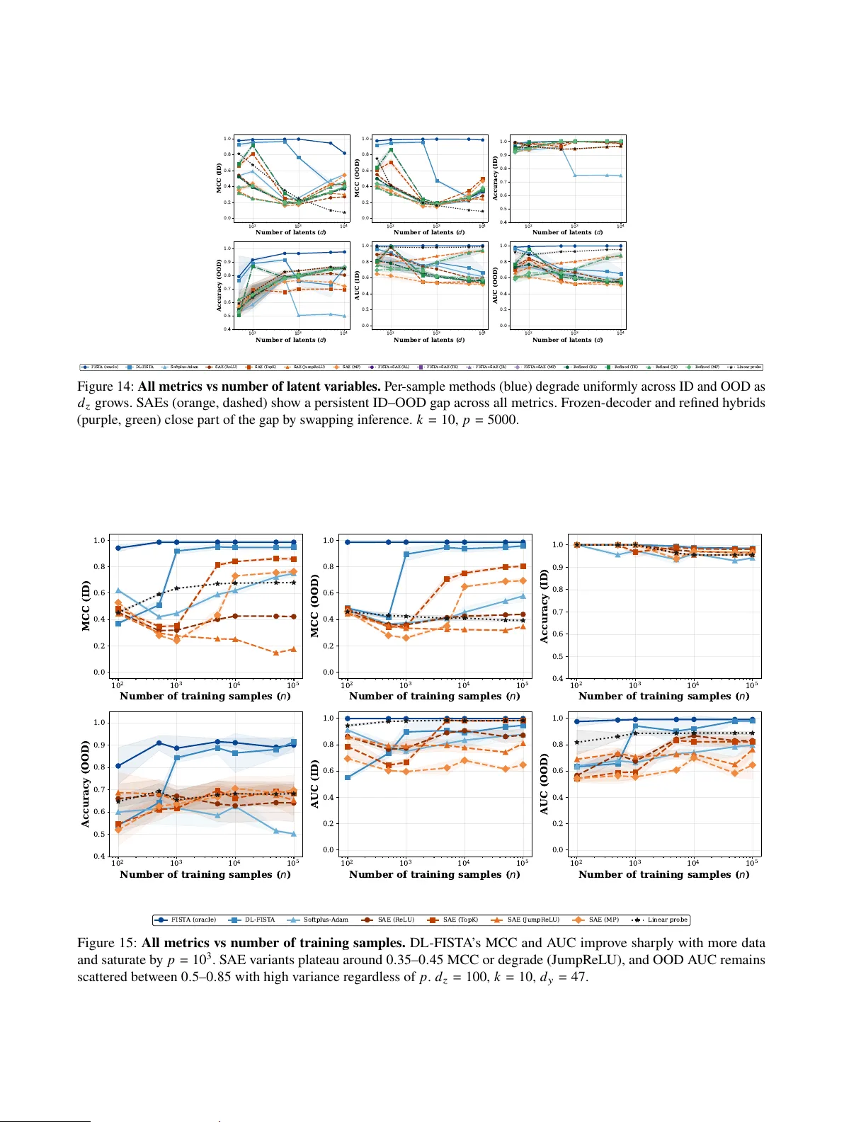
Stop Pr obing, Start Coding: Wh y Linear Pr obes and Sparse A utoencoders F ail at Compositional Generalisation Vit ´ oria Barin Pacela * 1 Shruti Joshi * 1 Isabela Camacho 2 Simon Lacoste-Julien 1 Da vid Klindt 3 * Equal contribution; authors listed in alphabetical order . 1 Mila - Qu ´ ebec AI Institute & U niversit ´ e de Montr ´ eal 2 Santa Clara U niv ersity 3 Cold Spring Harbor Laborator y Abstract The linear representation h ypothesis states that neural netw ork activ ations encode high-lev el con- cepts as linear mixtures. Ho w e v er , under super - position, this encoding is a projection from a higher -dimensional concept space into a low er - dimensional activation space, and a linear decision boundary in the concept space need not remain lin- ear after projection. In this setting, classical sparse coding methods with per -sample iterativ e inf erence le v erage compressed sensing guarantees to reco v er latent factors. Sparse autoencoders (S AEs), on the other hand, amortise sparse inference into a ﬁx ed encoder , introducing a sy stematic g ap. W e sho w this amortisation gap persists across training set sizes, latent dimensions, and sparsity le v els, caus- ing S AEs to f ail under out-of-dis tribution (OOD) compositional shifts. Through controlled e xper i- ments that decompose the failure, w e identify dic- tionar y learning —not the inf erence procedure—as the binding cons traint: S AE-learned dictionaries point in substantiall y wrong directions, and repla- cing the encoder with per -sample FIST A on the same dictionary does not close the gap. An oracle baseline pro v es the problem is sol vable with a good dictionary at all scales tested. Our results reframe the S AE failure as a dictionary lear ning c halleng e, not an amor tisation problem, and point to scalable dictionary lear ning as the k e y open problem f or sparse inf erence under superposition. 1 INTR ODUCTION U nderstanding the internal representations of Lar g e Lan- guage Models (LLMs) is crucial for their saf e and reliable deplo yment. The linear repr esentation hypothesis (LRH) is a f oundational assumption in mechanistic inter pretability , stating that a model’ s activ ations are linear mixtures of un- derl ying concepts ( Jiang et al. , 2024 ; Park et al. , 2024 ; Smith , 2024 ). It has motivated crucial progress on methods such as linear probing f or concept disco v ery and activation s teering ( T urner et al. , 2023 ; Chalnev et al. , 2024 ). T o make this precise, let z ∈ R 𝑑 𝑧 denote ground-tr uth lat- ent v ariables (concepts), and let y ∈ R 𝑑 𝑦 denote a model’ s activations. The LRH asser ts that the relationship betw een concepts and activ ations is linear: y ≈ Wz f or some matr ix W ∈ R 𝑑 𝑦 × 𝑑 𝑧 . The goal of inter pretability is to reco ver z from y —i.e., to inf er which concepts are activ e in an activ - ation v ector . When 𝑑 𝑧 > 𝑑 𝑦 , more concepts are encoded than there are activation dimensions, a regime kno wn as superposition ( Elhage et al. , 2022 ). The sys tem y = Wz is underdeter mined: each obser v ation y is consistent with inﬁnitely many z , so one cannot simply lear n a linear un- mixing to map activations bac k to concepts. In other w ords, linear r epr esentation —concepts being linear ly encoded in activations—is not the same as linear accessibility —that concepts are reco v erable by a linear transformation. How - ev er this distinction is routinel y o ver looked and the LRH is conﬂated with the much s tronger latter claim. Concept reco v er y requires additional structure to resolv e the underdetermination, such as b y assuming sparsity , i.e., in practice, onl y 𝑘 ≪ 𝑑 𝑧 concepts are activ e in any given input. Compressed sensing is precisely the framew ork that characterises when sparse signals can be reco vered from such underdetermined measurements ( Donoho and Elad , 2003 ; Donoho , 2006a ). Under the sparsity assumption, classical results sho w that 𝑘 -sparse codes can be reco v ered from 𝑑 𝑦 = O ( 𝑘 log ( 𝑑 𝑧 / 𝑘 ) ) input dimensions via nonlinear algorithms (e.g., basis pursuit, iterativ e thresholding), while requir ing reco v ery to be linear (e.g., a sparse linear probe) increases the required number of dimensions to 𝑑 𝑦 = 𝛺 𝜖  𝑘 2 log 𝑘 log  𝑑 𝑧 𝑘   ( Garg et al. , 2026 ), a quadratic blowup in 𝑘 . Concretely , f or 𝑑 𝑧 = 10 6 latent concepts with 𝑘 = 100 activ e at once, nonlinear recov er y requires only 𝑑 𝑦 ≈ 920 dimensions while linear reco v ery requires 𝑑 𝑦 ≈ 20 , 000 —a typical transformer hidden size of 4096 comf or tabl y e x ceeds the f ormer but falls f ar shor t of the latter . Thus, whether concepts are recov erable from a ﬁx ed set of activ ations theref ore depends not on whether the y are linearl y encoded, but on how one attempts to decode them. A dditionally , with respect to do wnstream implications, the compression through W f olds distinct regions of the latent space onto one another , so that a decision boundary that is linear in z -space can become nonlinear in y -space (Fig- ure 1 ). R ecov er ing z from y theref ore requires nonlinear methods, but which nonlinear method matters. Amor tised inf erence ( Gregor and LeCun , 2010 ), as implemented b y Sparse A utoencoders (S AEs) ( Ng et al. , 2011 ; Cunningham et al. , 2023 ), lear ns a ﬁxed encoder 𝑟 : R 𝑑 𝑦 → R 𝑑 ℎ that maps an activation to a sparse code in a single f orward pass by training on a ﬁnite distribution of training data. P er -sample inf er ence , b y contrast, sol v es an optimisation problem from scratch f or each input, using onl y the observation y and the dictionary W , with no dependence on a training distribution. Amortisation gap. The solution lear ned via amor tised or per -sample inf erence can be ev aluated b y ho w accuratel y either recov ers the tr ue sparse code, e.g., whether the cor - rect concepts are identiﬁed as active. In-distribution, both approaches may recov er z w ell, and the discrepancy between them—the amortisation gap ( Margossian and Blei , 2023 ; Kim and Pa vlo vic , 2021 ; Zhang et al. , 2022 ; Cremer et al. , 2018 ; Schott et al. , 2021 ; P aiton et al. , 2020 ; O’Neill et al. , 2024 )—can be small. U nder distribution shift, how ev er, the gap widens: when the sparsity pattern changes (e.g., no v el combinations of concepts co-activate), the amor tised en- coder’ s reco very degrades because it was optimised for training-time statis tics, while per -sample methods that optim- ise from scratch for each input remain unaﬀected. This paper studies the amortisation g ap in the conte xt of interpretability under superposition: U nder what conditions does spar se inf er ence r e- cov er the true latent f actor s from superposed ac- tivations, and how does the c hoice of inf erence procedur e—amortised, per -sample, or hybrid— aﬀect robus tness under distribution shift? This argument adds nuance to recent studies sugges ting that linear probes trained on top of LLM activations are superior to S AEs in out-of-dis tribution (OOD) binar y classiﬁcation tasks ( Kantamneni et al. , 2025 ). W e argue that the recent OOD failures of SAEs are not an indictment of the super - position hypothesis, but rather a predictable consequence of replacing principled sparse inference with a brittle, amor t- ised encoder . Instead of discarding the pow er ful frame work of sparse coding, w e embrace the geometric consequences of super position and utilize methods equipped to handle the nonlinearity it induces. Main contributions. In this work, we re visit classical sparse coding to address the central question. W e sho w that under superpos ition, e v en labels that are linearl y separable in latent space ma y become nonlinearl y separable in activ ation space. W e demonstrate that this is particularl y pronounced in OOD settings, so that a perfect linear probe trained in-distribution will f ail OOD (Figure 1 ). S AEs perform nonlinear inf erence, but amor tising it into a ﬁxed encoder introduces a sys tematic amortisation gap (Figure 5 ): the encoder ﬁts the training dis- tribution’ s co-occur rence s tructure and f ails to generalise to no v el combinations of latent factors under OOD composition shift (Figure 3 ). An oracle baseline—per -sample FIST A with the ground-tr uth dictionary—achie ves near -per f ect OOD re- co v ery at all scales tested, pro ving the problem is sol v able under compressed sensing theor y (Section 4 ). Through con- trolled e xper iments that decompose the S AE f ailure, we identify dictionary lear ning—not the inf erence procedure— as the binding constraint. S AE-lear ned dictionaries point in substantiall y wrong directions, and replacing the encoder with per -sample FIST A on the same dictionar y does not close the gap (F igure 8 ). Classical dictionary lear ning (DL- FIST A) produces better dictionaries at small scale, but both methods f ail at dictionary learning when the latent dimen- sion grow s large. These results reframe the S AE f ailure: the bottleneck is not amortisation of inference but amortisation of dictionar y lear ning, and the path f orward requires scalable algorithms for learning dictionaries under the compressed- sensing frame w ork. 2 RELA TED W ORK Compositional generalisation—the ability to understand and produce no v el combinations of lear ned concepts—remains a fundamental c halleng e for neural netw orks ( Fodor and Py ly shyn , 1988 ; Hupkes et al. , 2020 ). Current approaches in causal representation learning attempt to achie v e this through structural constraints, such as additiv e decoders ( Lachapelle et al. , 2023 ) (e.g., in S AEs), or speciﬁc training objectiv es like compositional risk minimisation ( Mahajan et al. , 2025 ). These w orks f ocus on obtaining guarantees f or the composi- tional g eneralisation of disentangled models, while here, w e ev aluate the eﬀect of compositional shifts under superposi- tion. S AEs hav e recentl y emer ged as a primar y tool f or decompos- ing the inter nal activations of LLMs into inter pretable, mono- semantic f eatures ( Cunningham et al. , 2023 ). Despite their success in interpretability , their out-of-distribution (OOD) robustness is a gro wing concern. Recent ev aluations sugges t that S AEs trained on g eneral datasets often f ail to disco ver generalisable concepts across diﬀerent domains or lay ers ( Heindrich et al. , 2025 ), under perf or m compared to simple linear probes ( Kantamneni et al. , 2025 ), and remain brittle e v en when scaled ( Gao et al. , 2024 ). Interestingl y , this br ittle- ness is less pronounced in domain-speciﬁc applications, such as medical QA or pathology , where S AEs ha v e sho wn more z 1 z 2 y 1 y 2 (a) z 1 z 2 z 3 y 1 y 2 Classifier Explicit Not explicit (b) Figure 1: Binary classiﬁcation with 𝑡 = 1 𝑧 1 > 0 . 5 (green: not explicit, pur ple: explicit). (a) When 𝑑 𝑧 = 𝑑 𝑦 , the linear decision boundary in latent space remains linear after mixing y = Wz . (b) When 𝑑 𝑧 > 𝑑 𝑦 (o v ercompleteness) and 𝑧 sparse, we can project do wn into non-ov erlapping regions (i.e., compressed sensing is possible), but the decision boundary becomes nonlinear in activation space, making linear probes insuﬃcient. stable and biologically relev ant f eature transf er ( O’Neill et al. , 2025 ; Le et al. , 2024 ). These conﬂicting results motiv ate a more principled ev aluation of S AEs under distr ibution shifts ( Joshi et al. , 2025 ). Recent w ork has highlighted the limitations of S AEs in re- co v ering true latent variables ( O’N eill et al. , 2024 ; Paulo and Belrose , 2025 ). This s tands in contras t to the classical sparse coding frame w ork ( Olshausen and Field , 1996 ; Ran- zato et al. , 2007 ), whic h utilises iterativ e optimisation rather than a learned encoder to recov er latent variables. This iter - ativ e approach pro vides strong er theoretical guarantees f or the unique reco v ery of latents ( Hillar and Sommer , 2015 ; Le wicki and Sejno wski , 1997 ; Gr ibon v al et al. , 2015 ). In contrast to O’Neill et al. ( 2024 ), who e xplore diﬀerent in- distribution (ID) amortisation strategies, w e f ocus our ana- ly sis on downs tream tasks under OOD compositional shifts. Lastl y , literature on o v ercomplete independent component anal ysis ( Podosinnik ov a et al. , 2019 ; W ang and Seig al , 2024 ) e xplores identiﬁability where the number of latent variables e x ceeds the number of observed variables ( 𝑑 𝑧 > 𝑑 𝑦 ), though these models typicall y rel y on statis tical independence rather than sparsity . 3 AMOR TIS A TION V S POINTWISE SP ARSE INFERENCE AND COMPOSITION AL GENERALISA TION W e begin b y specifying the data-generating process. Consider latent v ariable vectors z ∈ R 𝑛 with at mos t 𝑘 non-zeros. A support set 𝑆 ⊆ [ 𝑛 ] is drawn ﬁrst to index these non-zero components f ollowing the process: 𝑆 ∼ 𝑝 𝑆 , 𝒛 ∼ 𝑝 ( 𝒛 | 𝑆 ) supp ( 𝑝 𝑆 ) ⊆ S 𝑘 : = { 𝑆 ⊆ [ 𝑛 ] : | 𝑆 | ≤ 𝑘 } , P ( z 𝑆 𝑐 = 0 | 𝑆 ) = 1 . (1) An unkno wn generativ e process 𝑔 maps latents to data, pro- ducing x : = 𝑔 ( z ) ∈ R 𝑑 𝑥 . Although z is unobserved, w e ha v e access to lear ned representations y : = 𝑓 ( x ) ∈ R 𝑑 𝑦 f or some ﬁx ed (encoding) function 𝑓 : R 𝑑 𝑥 → R 𝑑 𝑦 (e.g., an LLM activation map). Since the coordinates of y need not neces- sarily align with those of z , we ﬁt a representation model 𝑟 : R 𝑑 𝑦 → R 𝑑 ℎ estimating h : = 𝑟 ( y ) and another decoder 𝑞 : R 𝑑 ℎ → R 𝑑 𝑦 s.t. ˆ y : = 𝑞 ( h ) . Ideall y , h serves as a proxy f or z and when 𝑑 𝑧 is kno wn, w e can set 𝑑 ℎ = 𝑑 𝑧 , while 𝑑 𝑦 < 𝑑 𝑧 . W e refer to individual coordinates of h (one-dimensional subspaces of R 𝑑 ℎ ) as f eatures , and we seek features that correspond (approximatel y) to the latent coordinates z . T ypicall y , h is enf orced to be sparse, in line with Equation ( 1 ). In practice, S AEs ( Cunningham et al. , 2023 ) are commonly used to learn the autoencoder 𝑞 ◦ 𝑟 , where typically the decoder 𝑞 is assumed to be linear and the encoder 𝑟 is a single-linear la y er f ollow ed by an activ ation function such as ReL U ( Cunningham et al. , 2023 ), JumpR eLU ( Ra jaman- oharan et al. , 2024 ), or T opK ( Gao et al. , 2024 ; Costa et al. , 2025 ). The assumption of a linear decoder is motivated b y the LRH stating that the composed map 𝑓 ◦ 𝑔 is linear in the underl ying latent variables s.t., y = 𝑓 ( 𝑔 ( z ) ) ≈ Az + b , x ∼ 𝑝 x , (2) f or some matrix A ∈ R 𝑑 𝑦 × 𝑑 𝑧 and oﬀset b ∈ R 𝑑 𝑦 , where 𝑝 x denotes the induced data dis tribution under the generativ e process x = 𝑔 ( z ) . A long line of w ork pro vides e vidence f or this h ypothesis (c.f. Rumelhart and Abrahamson ( 1973 ); Hinton et al. ( 1986 ); Mik olo v et al. ( 2013 ); Ra vf ogel et al. ( 2020 ); Klindt et al. ( 2025 )). More recently , theoretical work justiﬁes wh y linear proper ties could ar ise in these models (c.f. Jiang et al. ( 2024 ); Roeder et al. ( 2021 ); Marconato et al. ( 2024 ); Reizing er et al. ( 2024 )). Ensuring injectivity under o v ercom pleteness. S AEs are often trained with an o v ercomplete f eature dimension 𝑑 ℎ > 𝑑 𝑦 , so that the decoder operates as a linear dictionary W ∈ R 𝑑 ℎ × 𝑑 𝑧 . When 𝑑 ℎ > 𝑑 𝑦 , the decoder dictionar y W ∈ R 𝑑 𝑦 × 𝑑 ℎ has more columns than ro w s, i.e. it is projecting from a high to a lo w-dimensional space, like projecting a 3D object onto its 2D shado w . This compression means there must e xist nonzero codes h f or whic h Wh = 0 (i.e. ker ( W ) ≠ { 0 } since dim ker ( W ) = 𝑑 ℎ − rank ( W ) ≥ 𝑑 ℎ − 𝑑 𝑦 > 0 ). Thus, inf ormation is ine vitably los t, so multiple codes h can produce the same activation y , resulting in its inﬁnitely man y possible reconstructions. This non-uniqueness has a deeper consequence in that there is nothing to identify since identifying a g round truth solution w ould imply presupposing its uniqueness. But, the model y = Wz is inherentl y not identiﬁabl y since, f or an y in v er tible ( 𝑑 𝑧 b y 𝑑 𝑧 ) matrix M , w e can write y = ( WM ) ( M − 1 z ) = W ′ z ′ , deﬁning a diﬀerent dictionar y and latent v ar iable that result in the same observ ed variable y . Thus, interpreting h = 𝑟 ( y ) as reco v ering latents requires an additional selection pr inciple that pref ers one solution among man y consistent codes. T o obtain a unique solution, one typically res tricts the code to be sparse, mir roring the latent sparsity assumption in Equation ( 1 ). Concretely , we restrict h ∈ R 𝑑 ℎ to lie in the 𝑘 -sparse set 1 : 𝛴 ( 𝑑 ℎ ) 𝑘 : = { h ∈ R 𝑑 ℎ : ∥ h ∥ 0 ≤ 𝑘 } , This sparsity can be enf orced softl y (e.g., via an ℓ 1 penalty) or as a hard cons traint through constrained optimisation ( Ramirez et al. , 2025 ; Gallego-Posada et al. , 2025 ), or as implemented in T opK S AEs, which retain onl y the 𝑘 larg est- magnitude coordinates of h per input. Algebraicall y , sparsity replaces the unconstrained f easibility set { h ∈ R 𝑑 ℎ : Wh = y } (typically inﬁnite) with the constrained set { h ∈ 𝛴 ( 𝑑 ℎ ) 𝑘 : Wh = y } , which can be a singleton under suitable conditions on W . In this sense, 𝑟 ( y ) is meaningful onl y insofar as it implements a consistent sparse selection of dictionary atoms among the man y codes that reconstruct the same y . Identiﬁability of sparse codes h . R estricting the codes to be sparse is not suﬃcient to guarantee uniqueness—there ma y still exis t distinct h , h ′ ∈ 𝛴 ( 𝑑 ℎ ) 𝑘 with Wh = Wh ′ . W e need a proper ty of the dictionar y W ensuring that it does not collapse sparse codes onto each other so that the y can be identiﬁable. A standard suﬃcient condition is the restricted isometry property (RIP) ( Candes and T ao , 2006 ; Donoho , 2006b ; Cand ` es and W akin , 2008 ): W satisﬁes RIP of order 𝑠 with constant 𝛿 𝑠 if ( 1 − 𝛿 𝑠 ) ∥ h ∥ 2 2 ≤ ∥ Wh ∥ 2 2 ≤ ( 1 + 𝛿 𝑠 ) ∥ h ∥ 2 2 ∀ ∥ h ∥ 0 ≤ 𝑠 . Intuitiv el y , W appro ximatel y preserves the g eo- metry of the sparse codes h , neither inﬂating nor collapsing them be y ond a tolerance determined by the number of non- zero components, i.e., sparsity 𝑠 of h . When w e consider h ∈ 𝛴 𝑑 ℎ 𝑘 , we want to ensure that tw o distinct 𝑘 -sparse codes h and h ′ are distinguishable, i.e., their diﬀerence is not in visible to W . Since, their diﬀerence can hav e at most 2 𝑘 non-zeros, this is equiv alent to asking that W maps no nonzero 2 𝑘 -sparse v ector to zero, since if Wh = Wh ′ , then W ( h − h ′ ) = 0 . RIP at order 2 𝑘 ensures ex actly this. 2 So, under RIP , it is im- 1 equiv alently requiring that supp ( h ) ∈ S ( 𝑑 ℎ ) 𝑘 : = { 𝑆 ⊆ [ 𝑑 ℎ ] : | 𝑆 | ≤ 𝑘 } . 2 A classical alternative is spark ( W ) > 2 𝑘 (spark of a matrix is possible f or tw o diﬀerent sparse v ectors to map to the same output since their diﬀerence cannot be in the null space of W , ensuring injectivity . RIP is fulﬁlled f or random Gaussian matrices projecting do wn into 𝑑 𝑦 ≥ O ( 𝑘 ln ( 𝑑 ℎ 𝑘 ) ) dimensions ( Cand ` es and W akin , 2008 ). Implica tion: How many concepts can we encode? The RIP bound 𝑑 𝑦 ≥ O ( 𝑘 ln ( 𝑑 ℎ / 𝑘 ) ) is logarit hmic in the dictionary size 𝑑 ℎ , meaning the number of latent concepts can be exponentiall y larger than the activation dimension. A typical value of a constant to realise the bound is 2 , i.e. 𝑑 𝑦 ≥ 2 ( 𝑘 ln ( 𝑑 ℎ / 𝑘 ) ) ( Baraniuk et al. , 2008 ). With 𝑑 𝑦 = 4 , 096 and 𝑘 = 50 activ e concepts, the bound permits dictionar ies as lar ge as 𝑑 ℎ ≈ 𝑒 𝑑 𝑦 / 2 𝑘 ∼ 𝑒 40 — astronomicall y more concepts than dimensions. Ev en conservativ ely , a transformer hidden size of 4 , 096 can in principle suppor t unique reco very o ver millions of latent concepts, pro vided onl y a f ew dozen are activ e at once. Thus, in the case of dictionar ies with up to 16 million f eatures on GPT - 4 activations ( Gao et al. , 2024 ), or 34 million f eatures with Claude 3 Sonnet ( T empleton , 2024 ), 𝑑 ℎ = 10 6 − 10 7 is still in the f easible range. The practical takea wa y is that scaling up the dictionary is essentiall y free from the perspectiv e of compressed sensing theor y . It is important to dis tinguish tw o lev els of identiﬁability that arise in this setting. The ﬁrst is code-level identiﬁability , i.e., giv en a ﬁxed and known dictionar y W , when can we uniquel y recov er the sparse code h from an obser v ation y . This is precisel y what RIP guarantees—it ensures that per - sample inf erence methods such as basis pursuit ( Chen et al. , 2001 ), or IST A ( Daubechies et al. , 2004 )/FIST A ( Beck and T eboulle , 2009 ) conv erg e to the uniq ue 𝑘 -sparse solution consistent with y . The second is dictionar y identiﬁability : can we recov er the dictionary W itself from obser v ations y ? Classical results sho w that W is identiﬁable when the data is suﬃcientl y sparse and div erse ( Hillar and Sommer , 2015 ; Gribon val et al. , 2015 ), whic h is similar to a more ﬂe xible suﬃcient support variability condition on data f or learning the dictionary ( Joshi et al. , 2025 ). These guarantees, ho w ev er , are only as useful as the optimisation procedure that realises them. Sparse Coding and Amortisation. Through point-wise inf erence, sparse coding inf ers a sparse code per input. Con- cretely , giv en samples { y 𝑖 } 𝑝 𝑖 = 1 and ﬁx ed dictionary W , the canonical pointwise f or mulation sol v es, f or each 𝑖 , h ★ 𝑖 ∈ arg min h ∈ R 𝑑 ℎ 1 2 ∥ y 𝑖 − Wh ∥ 2 2 + 𝜆 ∥ h ∥ 1 , (or equiv alentl y , a hard sparsity constraint h ∈ 𝛴 ( 𝑑 ℎ ) 𝑘 ). the smallest number of its columns that are linear ly dependent), no linear combination of 2 𝑘 or f ew er columns can weighted by W can sum to zero, i.e., ker ( W ) ∩ 𝛴 ( 𝑑 ℎ ) 2 𝑘 = { 0 } and hence W is injectiv e on 𝛴 ( 𝑑 ℎ ) 𝑘 ( Donoho and Elad , 2003 ; Gribonv al and Nielsen , 2004 ). But spark is typically intractable to compute. z 2 z 1 z 3 y 1 y 2 T rain (ID) T est (OOD) Figure 2: Compositional OOD split. Lef t : In-distribution (ID) training data co v ers suppor t pairs ( 𝑧 1 , 𝑧 2 ) and ( 𝑧 2 , 𝑧 3 ) and the no v el combination ( 𝑧 1 , 𝑧 3 ) is held out f or OOD ev aluation. Right : Same split in activation space y = Wz . Algorithms such as Iterative Shrinkage- Thresholding Al- gorithm (IS T A) and FIS T A compute h ★ 𝑖 b y iterating a se- quence of code estimates h ( 0 ) 𝑖 , h ( 1 ) 𝑖 , . . . f or each in put, typic- ally starting from h ( 0 ) 𝑖 = 0 and appl ying repeated gradient- and-thresholding updates until con ver g ence ( Beck and T e- boulle , 2009 ; Daubechies et al. , 2004 ). When the dictionar y is unknown, inf erence is paired with dictionar y learning ( Olshausen and Field , 1996 ; Mairal et al. , 2010 ), to alternate between (i) estimating { h 𝑖 } 𝑝 𝑖 = 1 giv en the current W and (ii) updating W to minimise reconstr uction er- ror under a column-norm constraint. A s tandard f or mulation is, min W , { h 𝑖 } 𝑝 𝑖 = 1 𝑝  𝑖 = 1  1 2 ∥ y 𝑖 − Wh 𝑖 ∥ 2 2 + 𝜆 ∥ h 𝑖 ∥ 1  s.t. ∥ W : , 𝑗 ∥ 2 ≤ 1 ∀ 𝑗 ∈ [ 𝑑 ℎ ] . (3) Implica tion: How sp arse must the codes be? 𝑘 enters the RIP bound roughly linearl y , denoting the number of inter pretable concepts simultaneously en- coded in the activation v ector . It is unclear a pr iori what the e xpected value of 𝑘 w ould be across diﬀerent ac- tivations. Rearranging the bound giv es the maximum f easible sparsity: 𝑘 max ≈ 𝑑 𝑦 / ln ( 𝑑 ℎ / 𝑘 ) . For 𝑑 𝑦 = 4 , 096 and 𝑑 ℎ = 10 7 , this yields 𝑘 max ≈ 185 , depending on the constant. Be yond this, no inf erence procedure—per - sample or amortised—can guarantee unique reco very . The choice of 𝑘 in training SAEs theref ore has implic- ations bey ond the reconstruction–sparsity trade-oﬀ as it determines whether the problem is ev en theoretically sol vable. In contrast, amor tised methods replace per -input iterative sol ving with a feed-f or w ard encoder that predicts h in a single forw ard pass, learning to appro ximate the solution across a training distribution( V afaii et al. , 2024 , 2025 ). W e can ha v e amortised sparse inference (e.g., LIST A ( Gregor and LeCun , 2010 )) that unrolls IST A iterations into lear n- able la y ers, so that its architecture is s tructurally tied to the sparse-coding objectiv e and the dictionary is treated as giv en. S AEs, the dominant amortised approach in inter pretability , are amortised autoencoding: they jointl y learn both the en- coder and the dictionary (the decoder 𝑞 ). An S AE encoder is free to learn any mapping that minimises recons tr uction loss on the training data, including solutions that exploit distributional shor tcuts rather than per f or ming pr incipled sparse decomposition. Implica tion: How to obtain sp arse codes? In the fully unsupervised setting assumed while training S AEs, there is no guarantee that the under l ying latent codes are sparse enough f or reco v ery . This connects to a broader impossibility: Hyv ¨ arinen and Pa junen ( 1999 ); Locatello et al. ( 2019 ) sho w that fully unsupervised dis- entanglement is impossible without inductiv e biases on the model or the data. In the compressed-sensing framing, the required inductive bias is precisely suﬃcient sparsity: the data must be g enerated b y activ ations in v ol ving f e w enough concepts at once. Joshi et al. ( 2025 ) propose to le v erage concept shifts being sparser to eﬀectivel y automate the creation of suﬃcientl y sparse and div erse observations from model activ ations. In the fully unsupervised setting, the general impossibility of unsupervised identiﬁabilty implies typical SAEs ha ve been sho wn not to be identiﬁable ( O’Neill et al. , 2024 ). W e hy - pothesise that this is one reason f or the poor generalisation of S AEs OOD f ound in the literature ( Kantamneni et al. , 2025 ). In pr inciple, a disentangled g eneralisation should allo w f or better OOD generalisation on downs tream tasks ( Sch ¨ olk opf* et al. , 2021 )—but whether this promise holds in practice depends on the entire pipeline—from dictionar y quality , through the inference procedure, to the do wnstream task. In this paper , we focus on this do wnstream ques tion. W e operationalise the central question from Section 1 b y study- ing compositional distribution shifts (no vel combinations of known concepts) which decompose it into tw o testable research ques tions: i Is sparse inf erence e v en necessary? Linear probes out- performing SAEs on OOD tasks does not mean linear decoding is suﬃcient, it jus t means amortised inference is failing. Labels that are linearl y separable in latent space become nonlinear l y separable in activation space, and this nonlinear ity is e xposed precisel y under compositional shifts. Rather than abandoning sparse coding f or linear probes, we suggest the solution lies within the compressed- sensing framew ork —but the bottleneck ma y not be where one e xpects. ii What is the bottlenec k: inf erence or dictionary learn- ing? S AEs jointl y learn a dictionar y and an encoder . W e decompose their f ailure to ask whether per -sample inf er - ence with an SAE-learned dictionar y can close the gap, and if not, whether the dictionary itself—rather than the encoder —is the binding constraint. Compositional g eneralisation. W e ev aluate inf erred sparse z 1 0.0 0.2 0.4 0.6 0.8 1.0 z 2 0.0 0.2 0.4 0.6 0.8 1.0 z 3 0.0 0.2 0.4 0.6 0.8 1.0 T rue latent variables 1.0 0.5 0.0 0.5 1.0 y 1 0.75 0.50 0.25 0.00 0.25 0.50 0.75 y 2 P r ojection into neural space z 1 0.0 0.2 0.4 0.6 0.8 1.0 1.2 z 2 0.0 0.2 0.4 0.6 0.8 1.0 1.2 z 3 0.0 0.2 0.4 0.6 0.8 1.0 1.2 Sparse Autoencoder (S AE) z 1 0.0 0.5 1.0 1.5 2.0 2.5 3.0 z 2 0.0 0.5 1.0 1.5 2.0 2.5 z 3 0.0 0.5 1.0 1.5 2.0 2.5 Sparse Coding (SC) Figure 3: S AEs fail to reco v er latent variables under super - position, but sparse coding succeeds. T op left: Ground-tr uth latents ( 𝑑 𝑧 = 3 , 𝑘 = 2 ); colors denote activ e-variable com- binations. T op right: Activ ation space y = Wz ( 𝑑 𝑦 = 2 ); factors o v erlap after projection. Bo ttom left: SAE recon- struction; planes are not recov ered. Bottom right: Sparse coding reconstruction; latents are identiﬁed up to scaling. codes via a do wnstream binary prediction task, where the targ et 𝑡 depends on the latent z through 𝑡 = 𝑢 ( z ) ∈ { 0 , 1 } ; hence, predicting 𝑡 from h through ˆ 𝑡 = 𝑣 ( h ) is a s tandard su- pervised proxy f or testing whether h preserves task -relev ant inf or mation about z , such as by ﬁtting a logistic head on h and ev aluating it through the log-odds log Pr ( 𝑡 = 1 | h ) Pr ( 𝑡 = 0 | h ) = a ⊤ h + 𝑎 0 f or weights a . T rain and test sets diﬀer in whic h combinations of generativ e factors co-occur (F igure 2 ). In ter ms of supports 𝑆 ⊆ [ 𝑛 ] of the sparse latent z (cf. Equation ( 1 )), the ID data e x cludes a structured subset of suppor t patterns while the OOD data concentrates on those withheld combinations. E.g., consider 𝑘 = 2 , and three factors 𝑧 1 . 𝑧 2 , 𝑧 3 . The ID data contains sup- port pairs ( 𝑧 1 , 𝑧 2 ) and ( 𝑧 2 , 𝑧 3 while the combination ( 𝑧 1 , 𝑧 3 ) is held out f or OOD ev aluation (Figure 2 . A don ws tream label 𝑡 = 1 { 𝑧 1 > 0 . 5 } depends only on 𝑧 1 , but a model trained ID ma y learn a shor tcut: since 𝑧 1 alw ay s co-occurs with 𝑧 2 , pre- dictor a 𝑇 h + 𝑎 0 can achie v e high accuracy by trac king features correlated with 𝑧 2 instead of isolating 𝑧 1 itself. The OOD split breaks this shortcut by pairing 𝑧 1 with 𝑧 3 instead (F ig- ure 1 ). This f ollo ws the withheld-co-occurrence logic central to spurious-cor relation benchmarks like W aterbirds ( Sag a w a et al. , 2019 ). Ac hie ving OOD success therefore req uires the encoder to reco ver coordinates where the e vidence for 𝑡 re- mains stable across diﬀerent latent factor recombinations. Figure 3 illus trates a to y e xample e xample of this failure, where S AEs fail to reconstruct the OOD plane ( 𝑧 1 , 𝑧 3 ) , while sparse coding reconstructs all latents. 1 0 1 1.5 1.0 0.5 0.0 0.5 1.0 1.5 Latent 0, IID, acc=1.0000 1 0 1 1.5 1.0 0.5 0.0 0.5 1.0 1.5 Latent 0, OOD, acc=0.8457 Class 1 Class 2 Decision boundary 1 0 1 1.5 1.0 0.5 0.0 0.5 1.0 1.5 Latent 1, IID, acc=0.9180 1 0 1 1.5 1.0 0.5 0.0 0.5 1.0 1.5 Latent 1, OOD, acc=1.0000 1 0 1 1.5 1.0 0.5 0.0 0.5 1.0 1.5 Latent 2, IID, acc=1.0000 1 0 1 1.5 1.0 0.5 0.0 0.5 1.0 1.5 Latent 2, OOD, acc=0.8262 Figure 4: Linear probes fail OOD under o ver complete- ness. Each column sets 𝑡 = 𝑧 𝑖 . The linear classiﬁer ﬁts the ID decision boundary w ell, but the compression y = Az introduces nonlinearity that is only e xposed OOD, causing catastrophic g eneralisation failure (columns 1, 3) or , ev en, poor ID accuracy (column 2). Linear Probing under the LRH. When W is injective ( 𝑑 𝑧 ≤ 𝑑 𝑦 ), linear separability is inv ar iant: W can rotate or rescale latent space, but a label that is linear in z remains linear in y = Wz (Figure 1a ; also ( Gar g et al. , 2026 ) Fig. 1). Ho w e v er , under o vercompleteness, e ven labels that are lin- earl y separable in latent space can become nonlinearl y separ - able in activation space. When W is non-injectiv e, multiple z map to the same y , potentiall y l ying on opposite sides of the latent h yperplane; in that case, no linear r ule in y can match the latent separator without er ror . This is the geometric phe- nomenon illustrated in Figure 1 b: a h yper plane separator in the full latent space can appear linear on the in-distr ibution slice of observed mixtures, y et become eﬀectivel y nonlinear (or e ven ill-posed 3 ) in activation space after being trans- f or med through W . Figure 4 illustrates diﬀerent failure cases of linear probes under this compositional setting. Under sparse coding, RIP does not mak e W globally inv er tible, but it ensures that W does not collapse sparse directions, so that sparse latents remain (nonlinearl y) distinguishable and pointwise sparse inf erence is w ell-posed. 4 EXPERIMENTS W e in v estig ate tw o ques tions: (i) is the OOD failure of S AEs a fundamental limitation of sparse inference under super pos- ition, or is it a f ailure of speciﬁc components (dictionar y , encoder , or both)? (ii) If the problem is solv able in prin- ciple, what is the bottlenec k in practice? W e use an oracle baseline—FIST A with the g round-truth dictionary—to es- tablish an upper bound on what per -sample inference can achie ve, then progressiv ely decompose the gap betw een this oracle and S AEs. Methods span f our f amilies from fully 3 Ill-posedness ar ises when ∃ z ≠ z ′ with Wz = Wz ′ but 𝑡 ( z ) ≠ 𝑡 ( z ′ ) , in which case 𝑡 is not a function of y at all. T able 1: Ke y ratios. The bound requires 𝛿 ≥ 𝐶 𝜌 ln ( 1 / 𝜌 ) f or a cons tant 𝐶 > 0 : sparser codes (smaller 𝜌 ) and higher observation dimension (larg er 𝛿 ) mak e reco v er y easier . Symbol Deﬁnition Interpretation 𝜌 𝑘 𝑑 ℎ Sparsity . Fraction of non-zeros in h . 𝛿 𝑑 𝑦 𝑑 ℎ Undersam pling. Ratio of observation dimension 𝑑 𝑦 to code dimension 𝑑 ℎ . 𝛿 < 1 is the o v ercomplete regime. per -sample to fully amortised inference, plus a linear -probe baseline. All are ev aluated on both in-distr ibution (ID) and out-of-distribution (OOD) test sets, where the OOD split withholds speciﬁc combinations of activ e latents during train- ing (Figure 2 ). W e consider latent v ariables z ∈ [ 0 , 1 ] 𝑑 𝑧 with at most 𝑘 non-zero entr ies, each sampled uniformly on [ 0 , 1 ] when activ e, observed through a linear mixing y = Az , where A ∈ R 𝑑 𝑦 × 𝑑 𝑧 with 𝑑 𝑦 < 𝑑 𝑧 . Details in Section A . T w o ratios go v ern recov er y diﬃculty (T able 1 ): sparsity 𝜌 = 𝑘 / 𝑑 𝑧 and undersampling 𝛿 = 𝑑 𝑦 / 𝑑 ℎ . W e e v aluate these using the metrics below . The target 𝑡 = 1 { 𝑧 1 > 0 . 5 } is predicted from inf erred codes h . Metrics. W e report three quantities on both ID and OOD data (details in Section D.1 ). The mean correlation coeﬃcient ( MCC ) ( Hyvarinen and Mor ioka , 2016 ) e valuates identiﬁ- ability s.t. MCC = 1 f or a representation identiﬁed up to permutation and rescaling. Accuracy trains a logis tic probe on the inf er red codes h to predict the binary label 𝑡 , appl y- ing the same supervised classiﬁer to ev er y method’ s codes, isolating the eﬀect of the representation. A UC is computed per -feature without a trained classiﬁer: f or each code dimen- sion, w e use the ra w activation as a score and compute R OC A UC; the single best f eature on ID data is selected and its A UC is repor ted on both splits. A UC tests whether the label is isolated in an individual f eature—a stronger condition than accuracy , which can e xploit combinations of features. In the main te xt w e report MCC (identiﬁability) and Accuracy (f or fair do wnstream comparison between an unsupervised and a supervied lear ning method). A UC and additional metrics are in the appendix. Methods. W e compare methods spanning four f amilies: sparse coding (per -sample ℓ 1 inf erence with oracle or lear ned dictionaries), SAEs , frozen decoder (per -sample FIST A on a frozen S AE-lear ned dictionar y), and r eﬁned hybrids (FIS T A warm-started from SAE codes). The last two families dis- entangle dictionary quality from inf erence: frozen-decoder methods replace onl y the encoder while reusing the S AE’ s dictionary , whereas reﬁned methods additionall y test whether the S AE’ s output pro vides a useful initialisation. A linear - probe baseline (or, a super vised sky line) operates directly on y . Architectural and optimisation details are in C.1 . All S AEs (ReL U ( Cunningham et al. , 2023 ), JumpReL U ( Ra- jamanoharan et al. , 2024 ), T op-K ( Gao et al. , 2024 ), MP ( Costa et al. , 2025 )) share the same decoder dimension and are trained with identical optimiser settings, diﬀering only in the activ ation function go verning the encoder ’ s sparsity mechanism. 4.1 THE AMORTIS A TION GAP PERSISTS A CROSS UNDERS AMPLING RA TIOS Compressed sensing theory predicts a phase transition in sparse reco v ery: once the number of obser v ations 𝑑 𝑦 e x ceeds 𝑂 ( 𝑘 ln ( 𝑑 𝑧 / 𝑘 ) ) , per -sample ℓ 1 methods recov er the latent code e xactl y . W e sweep the undersampling ratio 𝛿 = 𝑑 𝑦 / 𝑑 ℎ across a grid of latent dimensions 𝑑 𝑧 ∈ { 50 , 100 , 200 } and sparsity lev els 𝑘 ∈ { 3 , 5 , 10 } , and report ID MCC (F igure 5 ). Phase transition with other metr ics are repor ted in Section D . If S AEs sol v ed the same sparse inf erence problem, they w ould e xhibit the same transition and reach the same asymp- totic performance. A persistent g ap betw een the tw o w ould rev eal the cost of amortising inference into a ﬁx ed encoder . Per -sample methods e xhibit the predicted phase transition. FIST A (oracle) transitions shar pl y to near -per f ect MCC once 𝛿 passes a critical threshold, and the transition sharpens with 𝑑 𝑧 , matching the theoretical prediction. The empirical transition point is consis tent with the cons tant 𝐶 ≈ 2 used in the compressed-sensing bound 𝛿 ≥ 𝐶 𝜌 ln ( 1 / 𝜌 ) , v alidating the bound’ s practical relev ance. DL -FIS T A f ollo w s the same curve, shifted right b y the cost of learning the dictionar y . S AE variants also improv e with 𝛿 —the y are not insensitiv e to the undersampling ratio—but plateau at 0 . 2 – 0 . 5 MCC, w ell belo w the near-perf ect reco very that per-sample methods achie v e in the same regime. Crucially , the g ap does not close at high 𝛿 , impl ying that e ven when the problem is well within the regime where compressed sensing guarantees e xact recov er y , the amor tised encoder remains the bottleneck. T ak ea wa y . Both S AEs and sparse coding beneﬁt from less aggressive undersampling (higher 𝛿 ), but S AEs saturate far belo w per -sample methods. 4.2 SCALIN G UP LA TENT DIMENSION DOES NOT CLOSE THE C OMPOSITIONAL G AP All unsupervised methods face a more c hallenging problem as 𝑑 𝑧 grow s, as the dictionar y has more columns and the space of sparse patter ns e xpands combinator iall y . W e hypothesise that per -sample methods should deg rade more gracefull y if the bottleneck is dictionary lear ning, whereas S AEs should degrade fas ter if the bottleneck is amortised inf erence. W e sweep 𝑑 𝑧 ∈ { 50 , 100 , 500 , 1K , 5K , 10K } with 𝑘 and 𝛿 held ﬁx ed and repor t ID MCC (Figure 6 ) and OOD accuracy (Figure 7 ). As 𝑑 𝑧 gro ws, dictionar y lear ning becomes harder 0.2 0.4 0.6 0.8 1.0 = d y / d z 0.0 0.2 0.4 0.6 0.8 1.0 MCC (ID) d z = 5 0 , k = 3 0.2 0.4 0.6 0.8 1.0 = d y / d z 0.0 0.2 0.4 0.6 0.8 1.0 MCC (ID) d z = 5 0 , k = 1 0 0.1 0.2 0.3 0.4 0.5 = d y / d z 0.0 0.2 0.4 0.6 0.8 1.0 MCC (ID) d z = 2 0 0 , k = 3 0.2 0.4 0.6 0.8 1.0 = d y / d z 0.0 0.2 0.4 0.6 0.8 1.0 MCC (ID) d z = 2 0 0 , k = 1 0 P er-sample methods exhibit a sharp phase transition; SAEs plateau at 0.2 0.5 MCC regardless of . FIST A (oracle) DL-FIST A SAE (T opK) SAE (ReL U) Linear probe Figure 5: The amortisation gap persists across under - sampling ratios. P er -sample methods (FIST A) e xhibit a sharp phas e transition to near -perfect MCC once 𝛿 e x ceeds the compressed-sensing threshold; SAEs plateau at 0 . 2 – 0 . 5 MCC regardless of 𝛿 . Each panel sho ws a diﬀerent ( 𝑑 𝑧 , 𝑘 ) combination. f or all unsupervised methods. W e include FIST A with the ground-tr uth dictionary as an upper bound: it sho ws what is achie vable with a perfect dictionary and isolates dictionar y learning as the variable under test. FIST A (oracle) remains near -per f ect (MCC ≥ 0 . 95 , OOD accuracy ≈ 0 . 97 ), conﬁrm- ing the problem is solv able at all scales. DL-FIST A degrades in MCC as 𝑑 𝑧 grow s—dropping to ∼ 0 . 3 b y 𝑑 𝑧 = 10K —but maintains a small ID–OOD gap, indicating that its failure is dictionary quality , not compositional generalisation. When dictionary lear ning succeeds ( 𝑑 𝑧 ≤ 500 ), DL-FIST A dom- inates the linear probe on OOD accuracy ( 0 . 92 vs 0 . 83 ). S AE codes oﬀer no consis tent advantag e ov er probing raw activations at any scale, consistent with Kantamneni et al. ( 2025 ). V arying sparsity 𝑘 with 𝑑 𝑧 ﬁx ed yields the same pattern (appendix, Figure 16 ). T ak ea wa y . The oracle pro v es the problem is sol vable at all scales—the OOD failure is not inherent to superposition. DL-FIST A beats linear probes when dictionar y learning succeeds ( 𝑑 𝑧 ≤ 500 ) but f alls behind at scale, conﬁr m- ing dictionary lear ning as the univ ersal bottleneck. S AE codes oﬀer no do wnstream adv antag e ov er raw activ ations, consistent with Kantamneni et al. ( 2025 ). 4.3 MORE D A T A DOES NOT CLOSE THE AMORTIS A TION GAP One issue with the e valuation setup could be that S AEs are simpl y data-limited: with enough training samples, the encoder should lear n to appro ximate per -sample inf erence. If this were the case, the gap betw een S AEs and sparse coding 1 0 2 1 0 3 1 0 4 N u m b e r o f l a t e n t s ( d z ) 0.0 0.2 0.4 0.6 0.8 1.0 MCC (ID) FIST A (oracle) DL-FIST A SAE (T opK) SAE (ReL U) Linear probe Scaling latent dimension does not close the compositional gap. Figure 6: Scaling latent dimension does not close the com- positional g ap. DL-FIST A degrades due to dictionar y learn- ing diﬃculty but maintains a small ID–OOD gap. S AEs plateau at 0 . 2 – 0 . 5 MCC. The linear probe deg rades sharply as super position intensiﬁes. 𝑘 = 10 , 𝑝 = 5000 , 𝑑 𝑦 f ollo ws the CS bound. 1 0 2 1 0 3 N u m b e r o f l a t e n t s ( d z ) 0.5 0.6 0.7 0.8 0.9 Accuracy (OOD) FIST A (oracle) DL-FIST A SAE (T opK) SAE (ReL U) SAE (JumpReL U) SAE (MP) Linear probe Same downstream probe on each method s codes: FIST A (oracle) dominates; SAEs match or trail linear probes. Figure 7: DL-FIST A beats linear probes when dictionary learning succeeds but falls behind at scale. OOD accuracy of a logistic probe trained on each method’ s codes. FIS T A (oracle) dominates at all scales. SAE codes oﬀer no advantag e o v er probing ra w activ ations. 𝑘 = 10, 𝑝 = 5000. w ould shrink as the training set g ro ws. W e vary the number of training samples 𝑝 ∈ { 10 2 , . . . , 10 5 } with all other parameters held ﬁx ed and repor t ID MCC (Figure 10 ) and OOD accuracy (F igure 11 ). FIST A (oracle) is constant b y constr uction (it uses no training data be y ond the oracle dictionar y). DL-FIST A beneﬁts substantiall y from more data—its MCC jumps from ∼ 0 . 5 at 𝑝 = 10 2 to ∼ 0 . 98 b y 𝑝 = 10 3 and saturates—conﬁrming that dictionary lear ning is g enuinely sample-limited and that per -sample inf erence e xploits a better dictionar y immediatel y . SAE v ariants show a diﬀerent pattern. SAE (T opK) and SAE (ReL U) improv e only mar ginall y , plateauing around 0 . 35 – 0 . 45 MCC. S AE (JumpReL U) degrades with more data, dropping from ∼ 0 . 45 to belo w 0 . 1 , sugg esting that additional training leads to a poor local solution rather than cor recting it. The gap between 1 0 2 1 0 3 1 0 4 N u m b e r o f l a t e n t s ( d z ) 0.0 0.2 0.4 0.6 0.8 1.0 MCC (ID) ReL U 1 0 2 1 0 3 1 0 4 N u m b e r o f l a t e n t s ( d z ) T opK 1 0 2 1 0 3 1 0 4 N u m b e r o f l a t e n t s ( d z ) JumpReL U 1 0 2 1 0 3 1 0 4 N u m b e r o f l a t e n t s ( d z ) MP Swapping the SAE encoder for FIST A on the same frozen dictionary does not close the gap to DL-FIST A: the SAE -learned dictionary is the bottleneck on ID MCC . SAE encoder FIST A (frozen dec) Refined (warm) DL-FIST A FIST A (oracle) Figure 8: The SAE-learned dictionary is the bottleneck, not the encoder . Each panel sho ws one S AE type. Swapping the S AE encoder f or FIST A on the same frozen dictionary (blue) or warm-star ting from S AE codes (green) does not close the gap to DL-FIST A (purple), which lear ns its o wn dictionar y . The oracle (gray dashed) conﬁrms the problem is sol vable. 𝑘 = 10, 𝑝 = 5000. 1 0 2 1 0 3 1 0 4 N u m b e r o f l a t e n t s ( d z ) 0.0 0.2 0.4 0.6 0.8 1.0 Accuracy (OOD) ReL U 1 0 2 1 0 3 1 0 4 N u m b e r o f l a t e n t s ( d z ) T opK 1 0 2 1 0 3 1 0 4 N u m b e r o f l a t e n t s ( d z ) JumpReL U 1 0 2 1 0 3 1 0 4 N u m b e r o f l a t e n t s ( d z ) MP Swapping the encoder for FIST A on the same frozen dictionary does not improve OOD accuracy: the dictionary is the bottleneck. SAE encoder FIST A (frozen dec) Refined (warm) DL-FIST A FIST A (oracle) Figure 9: Swapping the encoder does not impro v e OOD accuracy: the dictionary is the bottlenec k. Same lay out as Figure 8 . R eplacing the SAE encoder with FIST A on the same frozen dictionary yields no consistent accuracy g ain. The gap to DL -FIS T A conﬁrms that the dictionar y directions, not the inference procedure, limit OOD performance. 𝑘 = 10 , 𝑝 = 5000. per -sample and amor tised methods is stable or widening across tw o orders of magnitude of additional data. On the do wnstream prediction task (F igure 11 ), DL -FIS T A clearl y separates from the linear probe once 𝑝 ≥ 10 3 ( 0 . 88 vs 0 . 68 accuracy), while all S AE v ar iants trail the linear probe—this is the regime ( 𝑑 𝑧 = 100 ) where dictionary lear ning w orks, and it translates directly into better OOD generalisation. OOD A UC sho ws the same pattern (appendix, Figure 20 ). T ak ea wa y . Additional training data closes the dictionar y learning gap (beneﬁting DL -FIS T A) but does not close the amor tisation gap. When dictionary learning succeeds, DL - FIST A dominates linear probes on the same do wnstream task, whereas S AE codes trail linear probes regardless of number of training samples. 4.4 THE BOTTLENECK IS THE DICTION AR Y , NOT THE EN CODER The preceding e xper iments conf ound tw o potential sources of S AE failure: a poor dictionar y and poor inf erence. W e isolate these with controlled experiments that hold one component ﬁx ed while varying the other . Swapping the encoder does not close the gap. Giv en a 1 0 2 1 0 3 1 0 4 1 0 5 N u m b e r o f t r a i n i n g s a m p l e s ( p ) 0.0 0.2 0.4 0.6 0.8 1.0 MCC (ID) FIST A (oracle) DL-FIST A SAE (T opK) SAE (ReL U) SAE (JumpReL U) SAE (MP) Linear probe More data closes the dictionary learning gap (DL-FIST A improves) but not the amortisation gap (SAEs plateau or degrade). Figure 10: Mor e data closes the dictionary learning gap but not the amortisation gap. DL -FIS T A ’ s MCC jumps from ∼ 0 . 5 to ∼ 0 . 98 b y 𝑝 = 10 3 , conﬁr ming dictionar y learn- ing is sample-limited. S AEs plateau or degrade with more data, and the gap betw een per -sample and amor tised methods is stable across tw o orders of magnitude. 𝑑 𝑧 = 100 , 𝑘 = 10 , 𝑑 𝑦 = 47. trained S AE with decoder ˆ W and bias ˆ b , w e compare three inf erence strategies on the same tes t input y : 1. SAE encoder (baseline): a single forward pass, h = 𝑟 ( y ) . 2. Frozen decoder : FIST A on y − ˆ b using ˆ W as a ﬁx ed 1 0 2 1 0 3 1 0 4 1 0 5 N u m b e r o f t r a i n i n g s a m p l e s ( p ) 0.5 0.6 0.7 0.8 0.9 Accuracy (OOD) FIST A (oracle) DL-FIST A SAE (T opK) SAE (ReL U) SAE (JumpReL U) SAE (MP) Linear probe Same downstream probe on each method s codes: DL-FIST A matches the oracle once data suffices; SAEs trail linear probes. Figure 11: More data closes the gap f or DL -FIS T A but not for SAEs. OOD accuracy of a logistic probe on each method’ s codes. DL -FIS T A matches FIS T A (oracle) once 𝑝 ≥ 10 3 ( 0 . 88 vs 0 . 68 f or the linear probe). All S AE variants trail the linear probe regardless of data. 𝑑 𝑧 = 100 , 𝑘 = 10 , 𝑑 𝑦 = 47. dictionary , initialised from h ( 0 ) = 0 . 3. Reﬁned (w ar m-start): FIST A on the same frozen ˆ W , ini- tialised from h ( 0 ) = 𝑟 ( y ) . All three use the same dictionary—onl y the inf erence pro- cedure diﬀers. Figure 8 sho ws the comparison alongside DL-FIST A (which lear ns its o wn dictionar y independentl y). The result sho ws that S AE encoders ≈ frozen FIST A ≈ reﬁned ( ∼ 0 . 15 – 0 . 4 MCC), while DL -FIS T A (which learns its o wn dictionary via classical alternating minimisation) achie v es an MCC of ∼ 0 . 75 – 0 . 95 . This implies that sw apping the encoder f or per -sample inf erence on the same dictionar y does not meaningfully impro v e reco v ery . The S AE-learned dictionary itself is the binding constraint. This conclusion is robust to the choice of FIST A regular isation s trength 𝜆 : sw eeping 𝜆 across three orders of magnitude yields at most modest improv ements o v er the S AE encoder , far below the or - acle at ev er y 𝜆 (appendix, Section D.7 ). Note that DL -FIS T A also degrades at larg e 𝑑 𝑧 (to ∼ 0 . 3 at 𝑑 𝑧 = 10K , Section 4.2 ), reﬂecting the inherent diﬃculty of dictionary lear ning at scale—but it degrades unif ormly across ID and OOD, unlike S AEs which e xhibit a compositional g eneralisation failure. The linear probe, operating directly on y without sparse inf erence, degrades in MCC e v en f aster as superposition intensiﬁes (Figure 6 ), but maintains sur prisingly high do wn- stream accuracy (F igure 7 ) because it is super vised f or that speciﬁc task —a div erg ence that illustrates ho w single-task metrics can mask identiﬁability failure. At 100 FIST A iterations (suﬃcient for con ver gence of the con v e x Lasso objectiv e) w arm-star ting from S AE codes yields the same solution as cold-starting from zeros, conﬁrm- ing that the per -sample optimisation conv erges regardless of initialisation. The one ex ception is T opK, whose S AE de- coder ac hiev es ∼ 0 . 87 OOD MCC on its o wn (comparable to DL-FIST A at small 𝑑 𝑧 ), consistent with T opK’ s str ucturall y enf orced sparsity producing a more faithful dictionary . The dictionary fails because the columns point in the wrong directions. W e track cosine similarity between de- coder columns and ground tr uth during training (Figure 12 ) and decompose column-lev el errors at con ver g ence (Fig- ure 28 ). A t 𝑑 𝑧 = 100 , DL-FIST A conv erg es to high cosine ( > 0 . 9 ) while S AEs plateau earlier —the S AE optimisation landscape is harder e v en when the problem is tractable f or alternating minimisation. A t 𝑑 𝑧 = 5000 , neither method ﬁnds the right directions (cosine ∼ 0 . 2 – 0 . 35 ), implying that the S AE dictionaries do not o v erﬁt or drift, the y simpl y nev er conv erg e. Norm ratios remain ≈ 1 . 0 throughout, and re-normalising columns or substituting oracle norms does not impro v e MCC ( Figure 27 ). T opK is an outlier at small 𝑑 𝑧 (cosine 0 . 93 , 90% of columns close to ground tr uth at 𝑑 𝑧 = 100), but this advantag e vanishes at scale. Wh y the encoder fails: wr ong support. W e measure support reco v er y —whether the S AE activ ates the correct f eatures—b y comparing the binar y nonzero pattern of SAE codes agains t the ground truth (after Hungarian matching). At 𝑑 𝑧 = 5000 with true sparsity 𝑘 = 10 : R eLU activates ∼ 120 of 5000 f eatures (precision 0 . 009 ); JumpR eLU activ - ates ∼ 300 (precision 0 . 005 ). Ev en T opK, which activ ates the cor rect number of f eatures ( ∼ 10 ), selects almost entirel y wrong atoms (precision 0 . 03 ). Re-estimating magnitudes via least-sq uares on the S AE’ s support makes things w orse (Fig- ure 56 ), conﬁr ming the support itself is incor rect. At smaller 𝑑 𝑧 , T opK’ s support precision is substantiall y better ( 0 . 49 at 𝑑 𝑧 = 100 ; Figure 29 ), e xplaining its stronger perf ormance at small scale. T ak ea wa y . The gap betw een oracle and other methods seems to be a dictionary lear ning problem. S AEs fail at both dictionary lear ning and inf erence, but the dictionar y is the binding constraint: per -sample inf erence cannot rescue wrong column directions. At scale ( 𝑑 𝑧 = 5000 ), DL -FIS T A also fails at dictionary lear ning (cosine ∼ 0 . 25 ), con v erging to similar MCC as S AEs. 4.5 THE SAE DICTION AR Y IS A USEFUL ST ARTIN G POINT Although the S AE decoder is a poor standalone dictionary , it ma y still encode useful structure that accelerates diction- ary lear ning. W e test this b y using the S AE decoder as the initial dictionary for DL -FIS T A (unsupervised alter nating optimisation), compar ing agains t DL -FIS T A initialised from a random dictionary . Figure 13 sho ws con v erg ence cur v es at 𝑑 𝑧 = 100 , sw eeping the number of dictionary-update rounds. The S AE decoder pro vides a clear head start: f or T opK, w ar m-s tarting begins at OOD MCC 0 . 87 and reaches 0 . 94 within 5 rounds, while random initialisation starts at 0 . 30 and requires ∼ 50 rounds 0 100 200 300 400 500 Epoch / Round 0.0 0.2 0.4 0.6 0.8 1.0 Cosine similarity to ground truth ReL U 0 100 200 300 400 500 Epoch / Round T opK 0 100 200 300 400 500 Epoch / Round JumpReL U 0 100 200 300 400 500 Epoch / Round MP Dictionary Quality During Training (d = 100) SAE (ReL U) DL-FIST A Figure 12: DL-FIST A learns correct dictionary directions; S AEs do not. S AE decoder cosine to ground tr uth vs training epoch (coloured) and DL-FIST A dictionar y cosine v s outer round (gray dashed) at 𝑑 𝑧 = 100 . At lar g e 𝑑 𝑧 ( ≥ 5000 ), neither method con v erg es (Figure 36 ). to reach the same lev el. For R eLU and JumpR eL U , the ad- vantag e is smaller but consistent—the S AE decoder sav es ∼ 20 – 50 rounds of dictionary learning. Both initialisations con v erg e to the same ﬁnal MCC, conﬁrming that the S AE decoder biases the optimisation to ward the cor rect basin without trapping it in a suboptimal one. Encoder warm-start is marginal. W e also test whether the S AE encoder ’ s output pro vides a useful initialisation f or per -sample FIST A (with frozen dictionary). Since the Lasso objective is conv ex, cold-start and warm-start must con v erg e to the same optimum giv en suﬃcient iterations. A t 100 iterations, both yield identical MCC. At lo w iteration budgets ( 1 – 10 ), w arm-star ting from S AE codes pro vides a modest adv antage f or T opK but negligible beneﬁt f or other types (appendix, Figure 26 ). The practical value of the S AE encoder as a FIST A initialiser is limited. T ak ea wa y . At small 𝑑 𝑧 , the S AE decoder is a useful w ar m- start f or DL-FIST A, sa ving ∼ 50 dictionary-update rounds. At large 𝑑 𝑧 ( ≥ 5000 ), this advantag e vanishes—neither initialisation leads to a good dictionary . The practical path f or w ard requires better dictionary lear ning algorithms that scale, not just better initialisations. 5 CON CLUSION In this paper, we asked tw o questions: is sparse inference necessary under super position, and if so, what is the bottle- neck? Sparse inf erence is necessary . Under superposition, con- cepts are linearl y repr esented in activations but not linear l y accessible —decision boundaries that are linear in latent space become nonlinear after projection. Linear probes, ev en with oracle access to ground-truth latents, degrade shar pl y in identiﬁability as super position intensiﬁes (MCC < 0 . 1 at 𝑑 𝑧 = 10 , 000 ). Per -sample FIST A with the g round-truth dic- tionary achiev es near -perfect OOD reco very (MCC ≥ 0 . 83, accuracy ≥ 0 . 97 ) at all scales, pro ving the problem is solv - able within the compressed-sensing frame w ork. The bottlenec k is dictionary learning, not inf erence. SAE- learned decoder columns point in substantially wrong direc- tions, and replacing the encoder with per -sample FIST A on the same dictionary does not help—the dictionary itself is the binding constraint. On the same do wnstream task, in our e xperiments, S AE codes oﬀer no adv antag e ov er probing ra w activ ations. Classical dictionary lear ning (DL-FIST A) dominates linear probes when it succeeds ( 𝑑 𝑧 ≤ 1 , 000 ). The gap betw een oracle and the best unsuper vised method iden- tiﬁes scalable dictionary learning as the ke y open problem f or sparse inference under superposition. Ref erences Richard Baraniuk, Mark Dav enpor t, R onald De V ore, and Michael W akin. A simple proof of the restricted isometry property for random matrices. Constructiv e appr oxima- tion , 28(3):253–263, 2008. Amir Beck and Marc T eboulle. A fas t iterativ e shrinkage- thresholding algorithm f or linear in verse problems. SIAM journal on imaging sciences , 2(1):183–202, 2009. T renton Brick en, Adl y T empleton, Joshua Batson, Br ian Chen, A dam Jermyn, T om Coner ly , Nick T ur ner , Cem Anil, Carson Denison, and Amanda Askell. T o wards monosemanticity: Decomposing language models with dictionary lear ning. T r ansformer Cir cuits Thr ead , pag e 2, 2023. URL https://transformer- circuits. pub/2023/monosemantic- features . Emmanuel J. Candes and T erence T ao. Near -optimal signal reco v ery from random projections: Univ ersal encoding strategies? IEEE T ransactions on Inf or mation Theory , 52 (12):5406–5425, 2006. doi: 10.1109/TIT .2006.885507. Emmanuel J Cand ` es and Michael B W akin. An introduc- tion to compressive sampling. IEEE signal processing mag azine , 25(2):21–30, 2008. Sviatosla v Chalne v , Matthe w Siu, and Arthur Conmy . Im- 1 0 1 1 0 0 0 1 0 0 1 0 1 1 0 2 1 0 3 Dict update rounds 0.0 0.2 0.4 0.6 0.8 1.0 MCC (OOD) ReL U 1 0 1 1 0 0 0 1 0 0 1 0 1 1 0 2 1 0 3 Dict update rounds T opK 1 0 1 1 0 0 0 1 0 0 1 0 1 1 0 2 1 0 3 Dict update rounds JumpReL U 1 0 1 1 0 0 0 1 0 0 1 0 1 1 0 2 1 0 3 Dict update rounds MP Decoder W arm-Start Convergence (d = 5000) DL-FIST A (random) DL-FIST A (SAE decoder) Oracle Figure 13: The S AE decoder is a useful w arm-start for dictionary learning. Orange: DL-FIST A initialised from SAE decoder . Blue: DL -FIS T A from random dictionary . Gra y dashed: oracle. The S AE decoder provides a clear head s tart, especially for T opK, but both initialisations con v erg e to the same optimum. 𝑑 𝑧 = 5000 , 𝑘 = 10 . Results at other 𝑑 𝑧 in appendix. pro ving steering v ectors b y targ eting sparse autoencoder f eatures. arXiv pr eprint arXiv :2411.02193 , 2024. Da vid Chanin, T om ´ a ˇ s Dulka, and Adri ` a Gar riga- Alonso. Feature hedging: Correlated features break narrow sparse autoencoders. arXiv pr eprint arXiv :2505.11756 , 2025. Scott Shaobing Chen, Da vid L Donoho, and Mic hael A Saunders. A tomic decomposition by basis pursuit. SIAM r eview , 43(1):129–159, 2001. V al ´ erie Costa, Thomas Fel, Ekdeep Singh Lubana, Bahareh T olooshams, and Demba Ba. From ﬂat to hierarchical: Extracting sparse representations with matc hing pursuit. arXiv pr eprint arXiv :2506.03093 , 2025. Chris Cremer, X uechen Li, and David Duv enaud. Inf erence suboptimality in variational autoencoders. In Interna- tional conf er ence on mac hine learning , pages 1078–1086. PMLR, 2018. Hoagy Cunningham, Aidan Ew art, Log an Riggs, Robert Huben, and Lee Sharke y . Sparse autoencoders ﬁnd highl y interpretable f eatures in language models, 2023. URL https://arxiv.org/abs/2309.08600 . I. Daubechies, M. Defrise, and C. De Mol. An iterativ e thresholding algorithm f or linear in v erse problems with a sparsity constraint. Communications on Pur e and Applied Mathematics , 57(11):1413–1457, 2004. doi: 10.1002/cpa. 20042. Da vid L Donoho. Compressed sensing. IEEE T r ansactions on inf ormation theor y , 52(4):1289–1306, 2006a. Da vid L. Donoho. Compressed sensing. IEEE T ransactions on inf or mation theor y , 52(4):1289–1306, 2006b. Pub- lisher: IEEE. Da vid L Donoho and Mic hael Elad. Optimall y sparse rep- resentation in general (nonorthogonal) dictionar ies via l1 minimization. Pr oceedings of the National A cademy of Sciences , 100(5):2197–2202, 2003. Nelson Elhag e, T ristan Hume, Catherine Olsson, Nicholas Schief er, T om Henighan, Shauna Krav ec, Zac Hatﬁeld- Dodds, R obert Lasenb y , Da wn Drain, Carol Chen, Rog er Grosse, Sam McCandlish, Jared Kaplan, Dario Amodei, Mar tin W attenberg, and Christopher Olah. T o y Models of Super position, September 2022. URL http://arxiv. org/abs/2209.10652 . arXiv :2209.10652 [cs]. Jerr y A Fodor and Zenon W Py ly sh yn. Connectionism and cognitiv e architecture: A critical anal ysis. Cognition , 28 (1-2):3–71, 1988. Jose Gallego-P osada, Juan Ramirez, Meraj Hashemizadeh, and Simon Lacoste-Julien. Cooper: A Librar y f or Con- strained Optimization in Deep Learning. arXiv pr eprint arXiv :2504.01212 , 2025. Leo Gao, T om Dupr ´ e la T our , Henk Tillman, Gabriel Goh, Rajan T roll, Alec Radford, Ily a Sutske ver , Jan Leike, and Jeﬀrey Wu. Scaling and e valuating sparse autoen- coders, 2024. URL 2406.04093 . Nikhil Garg, Jon Kleinberg, and Kenn y Peng. Ho w many f eatures can a languag e model store under the linear rep- resentation h ypothesis?, 2026. URL https://arxiv. org/abs/2602.11246 . Karol Gregor and Y ann LeCun. Lear ning fas t appro xima- tions of sparse coding. In Proceedings of t he 27t h interna- tional conf erence on int ernational conf er ence on mac hine learning , pages 399–406, 2010. R ´ emi Gr ibon v al and Morten Nielsen. Sparse representations in unions of bases. IEEE transactions on Information theory , 49(12):3320–3325, 2004. R ´ emi Gribonv al, Rodolphe Jenatton, and Francis Bach. Sparse and spurious: dictionar y lear ning with noise and outliers, 2015. URL 1407.5155 . Lo vis Heindrich, Philip T orr, Fazl Barez, and V eronika Thost. Do sparse autoencoders generalize? a case s tudy of an- sw erability , 2025. URL 2502.19964 . Christopher J. Hillar and Friedrich T . Sommer . When can dictionary learning uniq uel y reco v er sparse data from sub- samples? IEEE T r ansactions on Inf ormation Theor y , 61 (11):6290–6297, 2015. doi: 10.1109/TIT .2015.2460238. Geoﬀre y E Hinton et al. Lear ning distributed representations of concepts. In Pr oceedings of the eight h annual conf er - ence of the cognitiv e science society , v olume 1, pag e 12. Amherst, MA, 1986. Dieuwke Hupkes, V erna Dankers, Mathi js Mul, and Elia Bruni. Compositionality decomposed: Ho w do neural netw orks g eneralise? Journal of Ar tiﬁcial Intellig ence Resear ch , 67:757–795, 2020. Aapo Hyvarinen and Hiroshi Morioka. Unsupervised feature e xtraction b y time-contrastiv e lear ning and nonlinear ica. Advances in neur al inf ormation processing sys tems , 29, 2016. Aapo Hyv ¨ arinen and Petteri Pa junen. Nonlinear independent component analy sis: Existence and uniq ueness results. N eural ne tw orks , 12(3):429–439, 1999. Yibo Jiang, Goutham Rajendran, Pradeep Ravikumar , Br y on Aragam, and V ictor V eitch. On the or igins of linear representations in larg e language models, 2024. URL https://arxiv.org/abs/2403.03867 . Shruti Joshi, Andrea Dittadi, S ´ ebastien Lachapelle, and Dhan y a Sridhar . Identiﬁable steering via sparse autoen- coding of multi-concept shifts, 2025. URL https: //arxiv.org/abs/2502.12179 . Subhash Kantamneni, Joshua Engels, Senthooran Ra jaman- oharan, Max T egmark, and Neel Nanda. Are sparse au- toencoders useful? a case study in sparse probing. arXiv pr eprint arXiv :2502.16681 , 2025. Min y oung Kim and Vladimir P a v lo vic. R educing the amor t- ization gap in variational autoencoders: A ba yesian ran- dom function approach. arXiv preprint arXiv :2102.03151 , 2021. Da vid Klindt, Char les O’Neill, Patrik Reizing er , Harald Maurer , and Nina Miolane. From super position to sparse codes: inter pretable representations in neural networks. arXiv pr eprint arXiv :2503.01824 , 2025. S ´ ebastien Lac hapelle, Divy at Maha jan, Ioannis Mitliagkas, and Simon Lacoste-Julien. Additiv e decoders f or latent variables identiﬁcation and car tesian-product e xtrapolation. In A. Oh, T . Naumann, A. Glober - son, K. Saenko, M. Hardt, and S. Levine, editors, Advances in N eural Information Pr ocessing Sy stems , v olume 36, pages 25112–25150. Curran Associates, Inc., 2023. URL https://proceedings.neurips. cc/paper_files/paper/2023/file/ 4ef594af0d9a519db8fb292452c461fa- Paper- Conferen ce. pdf . Nhat Minh Le, Ciyue Shen, Neel P atel, Chintan Shah, Dar pan Sangha vi, Blake Mar tin, Alfred Eng, Daniel Shenker , Har - shith Padig ela, Ra ymond Biju, Sy ed Ashar Ja ved, Jen- nif er Hipp, John Abel, Harsha Pokkalla, Sean Grullon, and Dinkar Juyal. Learning biologically relev ant f ea- tures in a pathology foundation model using sparse au- toencoders, 2024. URL 2407.10785 . Michael Lewic ki and T er rence J Sejnow ski. Lear n- ing nonlinear o vercomplete representations for eﬃcient coding. In M. Jordan, M. Kearns, and S. Solla, editors, Advances in Neur al Informa- tion Processing Syst ems , volume 10. MIT Press, 1997. URL https://proceedings.neurips. cc/paper_files/paper/1997/file/ 489d0396e6826eb0c1e611d82ca8b215- Paper. pdf . Francesco Locatello, Stef an Bauer , Mario Lucic, Gunnar Raetsch, Sy lv ain Gell y , Ber nhard Sc h ¨ olk opf, and Olivier Bachem. Challenging common assumptions in the un- supervised learning of disentangled representations. In international conf er ence on mac hine learning , pages 4114– 4124. PMLR, 2019. Divy at Maha jan, Mohammad Pezeshki, Charles Arnal, Ioan- nis Mitliagkas, Kartik Ahuja, and Pascal Vincent. Com- positional risk minimization, 2025. URL https:// arxiv.org/abs/2410.06303 . Julien Mairal, Francis Bac h, Jean Ponce, and Guillermo Sapiro. Online lear ning f or matrix factorization and sparse coding. Jour nal of Mac hine Lear ning Resear ch , 11(1), 2010. St ´ ephane G Mallat and Zhif eng Zhang. Matching pursuits with time-frequency dictionaries. IEEE T ransactions on signal processing , 41(12):3397–3415, 1993. Emanuele Marconato, S ´ ebastien Lachapelle, Sebastian W eichw ald, and Luigi Gresele. All or none: Identiﬁable linear properties of next-tok en predictors in language mod- eling. arXiv pr eprint arXiv :2410.23501 , 2024. Charles C Margossian and David M Blei. Amortized variational inf erence: When and wh y? arXiv pr eprint arXiv :2307.11018 , 2023. T omas Mik olov , W en-tau Yih, and Geoﬀre y Zw eig. Lin- guistic regularities in continuous space w ord representa- tions. In Lucy V anderwende, Hal Daum ´ e III, and Katrin Kirchhoﬀ, editors, Pr oceedings of the 2013 Conf erence of t he North American Chapt er of the Association f or Computational Linguistics: Human Languag e T echnolo- gies , pag es 746–751, Atlanta, Geor gia, June 2013. As- sociation f or Computational Linguistics. URL https: //aclanthology.org/N13- 1090/ . Andre w Ng et al. Sparse autoencoder . CS294A Lecture not es , 72(2011):1–19, 2011. Bruno A. Olshausen and David J. Field. Emer gence of simple-cell receptiv e ﬁeld proper ties b y learning a sparse code f or natural images. Natur e , 381(6583):607–609, 1996. doi: 10.1038/381607a0. Charles O’Neill, Alim Gumran, and Da vid Klindt. Compute optimal inf erence and pro v able amortisation g ap in sparse autoencoders. arXiv pr eprint arXiv :2411.13117 , 2024. Charles O’Neill, Mudith Jay asekara, and Max Kirkby . R esur - recting the salmon: Rethinking mec hanistic interpretabil- ity with domain-speciﬁc sparse autoencoders, 2025. URL https://arxiv.org/abs/2508.09363 . Dy lan M P aiton, Charles G Fry e, Sheng Y Lundquist, Joel D Bo w en, R y an Zarcone, and Br uno A Olshausen. Selectiv - ity and robustness of sparse coding netw orks. Jour nal of vision , 20(12):10–10, 2020. Kiho Park, Y o Joong Choe, and Victor V eitch. The lin- ear representation h ypothesis and the g eometr y of lar ge language models, 2024. URL abs/2311.03658 . Gon c ¸ alo Paulo and N ora Belrose. Sparse autoencoders trained on the same data lear n diﬀerent features. arXiv pr eprint arXiv :2501.16615 , 2025. Anastasia Podosinnik o va, Amelia P err y , Alex ander S. W ein, Francis Bach, Ale xandre d’ Aspremont, and Da vid Sontag. Ov ercomplete independent component analy sis via sdp. In Kamalika Chaudhur i and Masashi Sug- iy ama, editors, Pr oceedings of the T w enty-Second Inter - national Confer ence on Artiﬁcial Intellig ence and S tat- istics , v olume 89 of Proceedings of Mac hine Learning Resear c h , pages 2583–2592. PMLR, 16–18 Apr 2019. URL https://proceedings.mlr.press/v89/ podosinnikova19a.html . Senthooran Ra jamanoharan, T om Lieberum, Nicolas Son- nerat, Ar thur Conm y , Vikrant V arma, J ´ anos Kram ´ ar , and Neel N anda. Jumping ahead: Impro ving reconstruction ﬁdelity with jumprelu sparse autoencoders, 2024. URL https://arxiv.org/abs/2407.14435 . Juan Ramirez, Meraj Hashemizadeh, and Simon Lacoste- Julien. P osition: A dopt constraints o v er penalties in deep learning. arXiv preprint arXiv :2505.20628 , 2025. Marc’ Aurelio Ranzato, Y -Lan Boureau, and Y ann LeCun. Sparse f eature lear ning f or deep belief netw orks. In Advances in Neur al Information Processing Syst ems (N eurIPS) , v olume 20, 2007. URL https://papers. nips.cc/paper_files/paper/2007/hash/ 2270a5fc66d369cd6c85026c045563b0- Abstract. html . Shauli Ra vf ogel, Y anai Elazar , Hila Gonen, Michael T witon, and Y oav Goldberg. Null it out: Guarding protected at- tributes b y iterativ e nullspace projection. In Dan Jurafsky , Jo y ce Chai, Natalie Sc hluter , and Joel T etreault, editors, Pr oceedings of the 58th Annual Meeting of the Association f or Computational Linguistics , pag es 7237–7256, On- line, July 2020. Association f or Computational Linguist- ics. doi: 10.18653/v1/2020.acl- main.647. URL https: //aclanthology.org/2020.acl- main.647 . Patrik Reizing er, Alice Bizeul, Attila Juhos, Julia E V ogt, Randall Balestriero, Wieland Brendel, and Da vid Klindt. Cross-entrop y is all y ou need to in v er t the data g enerating process. arXiv pr eprint arXiv :2410.21869 , 2024. Geoﬀre y R oeder , Luk e Metz, and Durk Kingma. On lin- ear identiﬁability of lear ned representations. In Int er - national Conf er ence on Mac hine Learning , pages 9030– 9039. PMLR, 2021. Da vid E Rumelhart and Adele A Abrahamson. A model f or analogical reasoning. Cognitiv e Psyc hology , 5(1):1–28, 1973. Shiori Saga wa, P ang W ei Koh, T atsunor i B Hashimoto, and Percy Liang. Distributionally robust neural netw orks f or group shifts: On the importance of regular ization f or w orst- case g eneralization. arXiv preprint arXiv :1911.08731 , 2019. B. Sch ¨ olk opf*, F . Locatello*, S. Bauer , N. R. Ke, N. Kal- chbrenner , A. Go yal, and Y . Bengio. T ow ard causal representation lear ning. Proceedings of the IEEE , 109 (5):612–634, 2021. doi: 10.1109/JPR OC.2021.3058954. URL https://ieeexplore.ieee.org/stamp/ stamp.jsp?arnumber=9363924 . *eq ual contribu- tion. Lukas Schott, Julius V on K ¨ ug elgen, Freder ik T r ¨ auble, Peter Gehler , Chris Russell, Matthias Bethg e, Ber nhard Sch ¨ olk opf, Francesco Locatello, and Wieland Brendel. Visual representation lear ning does not generalize strongl y within the same domain. arXiv pr eprint arXiv :2107.08221 , 2021. Le wis Smith. The ’s trong’ feature h ypothesis could be wrong. AI Alignment Forum, A ugust 2024. URL https://www.alignmentforum. org/posts/tojtPCCRpKLSHBdpn/ the- strong- feature- hypothesis- could- be- wrong . [A ccessed 02-26-2026]. A dly T empleton. Scaling monosemanticity : Extracting in- terpr etable featur es fr om claude 3 sonnet . Anthropic, 2024. R obert Tibshirani. Regression shrinkage and selection via the lasso. Journal of the R oy al Statis tical Society Series B: Statistical Me thodology , 58(1):267–288, 1996. Ale xander Matt T urner , Lisa Thierg ar t, Ga vin Leech, David Udell, Juan J V azquez, Ulisse Mini, and Monte MacDiar - mid. S teering language models with activ ation engineer - ing. arXiv pr eprint arXiv :2308.10248 , 2023. Hadi V af aii, Dekel Galor, and Jacob Y ates. P oisson v ar i- ational autoencoder . Advances in N eural Inf or mation Processing Sy stems , 37:44871–44906, 2024. Hadi V af aii, Dek el Galor , and Jacob L Y ates. Brain-like variational inf erence. ArXiv , pages arXiv –2410, 2025. Ke xin W ang and Anna Seigal. Identiﬁability of ov ercomplete independent component analy sis, 2024. URL https: //arxiv.org/abs/2401.14709 . Mingtian Zhang, P eter Ha y es, and Da vid Barber . General- ization gap in amor tized inf erence. Advances in neural inf ormation processing sy stems , 35:26777–26790, 2022. A SYNTHETIC D A T A DET AILS W e generate the synthetic data as f ollo w s. W e generate a projection matrix 𝐴 ∈ R 𝑚 × 𝑛 with 𝑚 < 𝑛 , where the elements of A are dra wn from a s tandard Normal dis tribution, in agreement with the Restricted Isometr y Proper ty from compressed sensing. The ro w s of 𝐴 are normalized to hav e unit nor m. W e generate the latent v ariables 𝑧 ∈ [ 0 , 1 ] 𝑛 with 𝑘 non-zero components, where the non-zero components are sampled unif or ml y from [ 0 , 1 ] . The obser v ed variables are then generated as 𝑦 = 𝐴 𝑧 . When selecting which combinations of latent v ariables to be activ e, which 𝑘 out of 𝑛 , w e consider the particular ”out-of- v ar iable” case f or OOD g eneralizations, where some combinations of the variables are not a vailable in the training data. The number of OOD variables is 𝑛 / 2. Then, we consider tw o possibilities: • ID dat a : Divided into tw o cases: – The ﬁrst latent v ar iable is activ e and the other 𝑘 − 1 are drawn betw een the variables of indices [ 2 , 𝑛 / 2 ] . – The ﬁrst latent v ar iable is not activ e. The 𝑘 activ e indices are drawn from the f ool pool of indices [ 2 , 𝑛 ] . • OOD data : The ﬁrst latent variable is activ e and the other 𝑘 − 1 are dra wn between the v ariables of indices [ 𝑛 / 2 + 1 , 𝑛 ] . The training set consists of ID data, and the tes t set consists of OOD data. B TRAINING DET AILS W e implement the models in PyT orch and train them on a single NVIDIA A100 GPU . C SP ARSE INFERENCE METHODS FOR INTERPRET ABILIT Y Sparse autoencoders (S AEs) hav e become the dominant tool f or e xtracting inter pretable f eatures from neural netw ork representations ( Br ic ken et al. , 2023 ; Cunningham et al. , 2023 ). An SAE decomposes an activation y ∈ R 𝑑 𝑦 as y ≈ Dh , where D ∈ R 𝑑 ℎ × 𝑑 𝑦 is an o v ercomplete dictionary ( 𝑑 ℎ > 𝑑 𝑦 ) and h ∈ R 𝑑 ℎ is a sparse code whose nonzero entr ies identify the activ e f eatures. The quality of the inter pretation depends entirel y on the quality of h : if the codes are wrong, the resulting f eature attribution is wrong, regardless of reconstruction ﬁdelity . Standard S AEs compute codes in a single f eedf orward pass, h = 𝜎 ( W ⊤ ( y − 𝑏 pre ) + 𝑏 ) , where 𝜎 is ReL U or a top- 𝑘 or JumpReL U activation. This is an amortised appro ximation to the sparse inf erence problem h ∗ = arg min h 1 2 ∥ y − Dh ∥ 2 2 + 𝜆 ∥ h ∥ 1 , (4) which is the Lasso ( Tibshirani , 1996 ), a conv e x problem with a unique solution (under mild conditions on D ). The amor tisation gap h − h ∗ is a structured er ror that is larg est precisely when f eatures are cor related or hierarchicall y org anised ( Costa et al. , 2025 ; Chanin et al. , 2025 )—the regimes most rele vant to real neural netw ork representations. Belo w w e compare three inf erence strategies that mo ve progressiv ely closer to sol ving Equation ( 4 ): FIS T A, LIST A, and Matching Pursuit. The comparison f ocuses on properties that matter for interpretability rather than reconstruction. C.1 ALGORITHMS FIST A (F ast Iterative Shrinkag e- Thresholding). FIST A ( Beck and T eboulle , 2009 ) solv es Equation ( 4 ) by alternating a gradient step on the reconstruction loss with the proximal operator f or the ℓ 1 penalty (soft-thresholding 𝑆 𝜆 ), accelerated b y Nes tero v momentum. Let h ( 𝑡 ) denote the code estimate at iteration 𝑡 and q ( 𝑡 ) a momentum-e xtrapolated point: q ( 𝑡 ) = h ( 𝑡 ) + 𝑡 𝑘 − 1 𝑡 𝑘 + 1  h ( 𝑡 ) − h ( 𝑡 − 1 )  , (5) h ( 𝑡 + 1 ) = 𝑆 𝜂 𝜆  q ( 𝑡 ) − 𝜂 D ⊤ ( D q ( 𝑡 ) − y )  , (6) where 𝜂 ≤ 1 / ∥ D ⊤ D ∥ op is the step size. Ev ery iteration updates all 𝑑 ℎ coeﬃcients simultaneously . The suppor t (whic h atoms are activ e) is ﬂuid: a coeﬃcient can be dr iv en to zero by soft-thresholding at step 𝑡 and reviv ed at step 𝑡 ′ > 𝑡 . Con v erg ence to the global optimum is guaranteed at rate 𝑂 ( 1 / 𝑡 2 ) ( Beck and T eboulle , 2009 ). There are no learned parameters; the algorithm is fully determined b y D and 𝜆 . Practical no te. Precomputing W = I − 𝜂 D ⊤ D and b = 𝜂 D ⊤ y reduces each iteration to h ( 𝑡 + 1 ) = 𝑆 𝜂 𝜆 ( W h ( 𝑡 ) + b ) : a single matrix–vector multipl y plus elementwise thresholding, both fully batchable on GPU . LIST A (Learned IST A). LIST A ( Gregor and LeCun , 2010 ) takes the IST A update (i.e. Equation ( 6 ) without momentum) and untethers its parameters from D . Each la yer 𝑡 computes: h ( 𝑡 + 1 ) = 𝑆 𝜃 𝑡  W 𝑡 h ( 𝑡 ) + B 𝑡 y  , (7) where W 𝑡 ∈ R 𝑑 ℎ × 𝑑 ℎ , B 𝑡 ∈ R 𝑑 ℎ × 𝑑 𝑦 , and 𝜃 𝑡 ∈ R 𝑑 ℎ are fr ee par amet ers learned by bac kpr opag ation , independentl y at eac h la y er . In IST A, W 𝑡 = I − 𝜂 D ⊤ D , B 𝑡 = 𝜂 D ⊤ , and 𝜃 𝑡 = 𝜂𝜆 1 f or all 𝑡 ; LIST A relaxes these constraints, allo wing the netw ork to learn iteration-dependent acceleration. Empirically , LIST A matches FIST A ’s solution quality in 10–20 la yers rather than 100+ iterations ( Gregor and LeCun , 2010 ). Crucially , LIST A retains the structural proper ties of IS T A/FIST A: all coeﬃcients are updated jointly at ev er y la yer , soft- thresholding pro vides a continuous sparsity mec hanism, and the architecture is fully parallelisable across the batc h dimension. The dictionary D (or its lear ned analogue in W 𝑡 , B 𝑡 ) can be trained end-to-end. MP -SAE (Matching Pursuit S AE). MP-S AE ( Costa et al. , 2025 ) unrolls the classical matching pursuit algor ithm ( Mallat and Zhang , 1993 ) into a diﬀerentiable encoder . Let d 𝑗 denote the 𝑗 -th column of D . At eac h step 𝑡 = 1 , . . . , 𝑇 : 𝑗 ( 𝑡 ) = arg max 𝑗 ∈ { 1 , .. ., 𝑑 ℎ } d ⊤ 𝑗 r ( 𝑡 − 1 ) , (8) ℎ 𝑗 ( 𝑡 ) = d ⊤ 𝑗 ( 𝑡 ) r ( 𝑡 − 1 ) , (9) r ( 𝑡 ) = r ( 𝑡 − 1 ) − ℎ 𝑗 ( 𝑡 ) d 𝑗 ( 𝑡 ) , (10) where r ( 0 ) = y − 𝑏 pre . One atom is selected per step; its coeﬃcient is computed by projection onto the residual; the residual is updated b y subtracting the selected atom’ s contr ibution. Pre vious coeﬃcients are nev er revised. The dictionary is trained end-to-end via backpropag ation through the unrolled steps. MP -SAE appro ximately sol v es a diﬀerent problem from Equation ( 4 ): it targets min h ∥ y − D h ∥ 2 2 subject to ∥ h ∥ 0 ≤ 𝑇 , which is NP -hard; matching pursuit is a greedy approximation with no global optimality guarantee. C.2 COMP ARISON ON INTERPRET ABILIT Y -RELEV ANT AXES W ell-posedness of codes. FIST A computes the uniq ue minimiser of the Lasso objectiv e Equation ( 4 ). The codes are deﬁned by a con v ex optimisation problem: one can point to the objectiv e and state precisel y what the codes mean. LIST A appro ximates this same solution with learned acceleration. MP -S AE computes the output of a greedy procedure that does not correspond to the global minimum of any ﬁx ed objectiv e; the codes depend on the selection order , which is itself a function of the dictionary g eometry and the input. For identiﬁability — where “meaning” is in variance across the eq uivalence class of valid solutions — the dis tinction matters: the Lasso solution is unique and characterisable; the MP output is not. Joint coeﬃcient adjustment. FIST A and LIST A update all 𝑑 ℎ coeﬃcients at ev er y iteration. If activ ating atom 𝑖 chang es the optimal coeﬃcient f or atom 𝑗 (as occurs whenev er d ⊤ 𝑖 d 𝑗 ≠ 0 ), subsequent iterations correct for this. MP -S AE sets each coeﬃcient once, at the step the atom is selected, and ne ver re vises it. Consider y = 𝛼 1 d 1 + 𝛼 2 d 2 with d ⊤ 1 d 2 = 𝜌 > 0 . MP selects d 1 ﬁrst (assuming 𝛼 1 > 𝛼 2 ) and assigns ℎ 1 = d ⊤ 1 y = 𝛼 1 + 𝛼 2 𝜌 , which is inﬂated b y d 2 ’ s contr ibution leaking through the correlation. The coeﬃcient ℎ 2 computed on the residual is correspondingly deﬂated. FIS T A con v erg es to the correct ( 𝛼 1 , 𝛼 2 ) because it jointly adjusts both coeﬃcients across iterations. Support dynamics. In FIST A/LIST A, the active set (support of h ) is ﬂuid: an atom can be activated, deactiv ated, and reactivated across iterations as the algorithm conv erges. This self-cor rection is critical when the initial support estimate is wrong. In MP -S AE, the support gro ws monotonicall y — once an atom is selected, it remains active. There is no mechanism to deselect an incorrectly chosen atom, and the error propagates through all subsequent residuals. Correlated and hierarc hical features. Standard S AEs compute all inner products ⟨ d 𝑗 , y ⟩ simultaneously and threshold, making all activation decisions in parallel. This implicitly assumes quasi-orthogonality of the dictionar y ( Cos ta et al. , 2025 ): if d 𝑖 and d 𝑗 are correlated, activating d 𝑖 should reduce the evidence f or d 𝑗 , but the one-shot encoder cannot e xpress this. MP -S AE ﬁx es the conditioning problem via the residual update Equation ( 10 ): after selecting d 𝑖 , atom d 𝑗 is ev aluated agains t the residual r rather than the raw in put, so correlated atoms no longer double-count shared v ar iance. This is also wh y MP -SAE naturall y reco vers hierarc hical structure: the ﬁrst iteration selects the dominant (coarse) f eature, and subsequent iterations select progressivel y ﬁner features on the residual. FIST A/LIST A handle cor related f eatures correctly and with cor rect magnitudes, because the joint coeﬃcient update av oids the inﬂation eﬀect described abo v e. Ho we v er, they do not pro vide a natural order ing o v er f eatures — all coeﬃcients con v erg e simultaneously rather than being produced in sequence. When a hierarchy readout is desired, the con v erg ence order or coeﬃcient magnitude in FIST A can ser v e as a proxy , but the sequential atom selection in MP pro vides this more directly . Computational cost. T able 2 summar ises the per -step and total cost f or a batch of 𝐵 samples. FIST A and LIST A are fully parallelisable across the batch; MP -S AE’ s sequential atom selection (the arg max in Equation ( 8 ) depends on the pre vious step’ s residual) limits GPU utilisation. LIST A compensates for its per -step cost b y conv erging in far f ew er steps than FIST A. T able 2: Computational compar ison of sparse inf erence methods. 𝑑 𝑦 : input dimension, 𝑑 ℎ : dictionary size, 𝑇 : number of steps/la yers, 𝐵 : batch size. FIST A LIST A MP -S AE Per -step cos t 𝑂 ( 𝐵 𝑑 2 ℎ ) 𝑂 ( 𝐵 𝑑 2 ℎ ) 𝑂 ( 𝐵 𝑑 ℎ ) T ypical steps 𝑇 100–300 10–20 𝑘 (activ e atoms) GPU parallelism Full Full Limited End-to-end trainable No 4 Y es Y es T rainability . LIST A and MP -SAE are both end-to-end trainable: the dictionary is updated by bac kpropag ation through the unrolled inf erence steps, using standard deep learning optimisers. FIST A requires alternating optimisation — an outer loop updating D and an inner loop running FIST A to con v erg ence for eac h batch — whic h is slo wer but pro vides stronger guarantees on code optimality . A practical middle ground is to train the dictionar y using a standard S AE or LIST A, then compute codes at ev aluation time using FIST A with the lear ned dictionary , optionally warm-started from the encoder’ s output. D EXPERIMENT AL RESUL TS D.1 METRIC DEFINITIONS AND WHA T EA CH DIA GNOSTIC ISOLA TES W e use three lev els of ev aluation metrics, each isolating a diﬀerent component of the S AE pipeline. T able 3 summarises the distinctions. T able 3: Summar y of e v aluation metrics and the questions the y answ er . Metric Operates on Question it answ ers MCC Codes vs z (samples) Do learned code dimensions track the same variation as the true latents, up to permutation and rescaling? A ccuracy Probe on codes vs labels Does a logistic classiﬁer on the codes predict the label OOD? (Same classiﬁer f or all methods—fair comparison.) Per -f eature A UC Codes v s labels (samples) Does a single code dimension separate the binary label? Cosine similarity Decoder ˆ W vs A (w eights) Do the dictionary atoms point in the same directions as the ground-tr uth columns? Norm ratio Decoder ˆ W vs A (w eights) Are the dictionary atoms the cor rect magnitude? Support precision Codes vs z (per -sample binary) Of the features the encoder activ ates, how man y are truly activ e? Support recall Codes vs z (per -sample binary) Of the tr ul y activ e f eatures, ho w many does the encoder ﬁnd? A ccuracy vs A UC: f airness considerations. The linear -probe baseline uses super vised r idg e regression from y to the ground-tr uth z , producing 𝑑 𝑧 -dimensional codes where each dimension is explicitl y trained to track one latent. P er-f eature A UC directl y beneﬁts from this alignment: each output dimension is already optimised to separate its targ et, giving the linear 4 FIST A itself is not trained; the dictionar y is updated in a separate alter nating minimisation s tep. How ev er , FIST A can be used at ev aluation time with a dictionar y trained b y an y method, including an S AE. probe an inherent adv antage o v er unsupervised methods whose code dimensions need not cor respond to individual latents. A ccuracy—training a logis tic probe on each method’ s inf erred codes—provides a f airer comparison because it applies the same do wnstream classiﬁer to all methods and can exploit f eature combinations, not just individual dimensions. In the main te xt w e theref ore repor t accuracy f or downs tream comparisons and reser v e A UC f or the appendix. MCC (end-to-end). The mean correlation coeﬃcient ( Hyv arinen and Morioka , 2016 ) computes the Pearson cor relation betw een each code column and each ground-truth latent column across samples, then ﬁnds the bes t one-to-one matching via the Hungarian algor ithm. It measures o verall reco very quality : MCC = 1 when codes reproduce the tr ue latents up to permutation and rescaling. P earson cor relation is in v ar iant to linear scaling, so MCC does not penalise magnitude diﬀerences. Ho w e v er , MCC conﬂates dictionar y q uality and encoder q uality—a low MCC does not tell y ou whether the dictionary atoms are wrong or the encoder is selecting the wrong atoms. Dictionary diagnostics (model-lev el). Cosine similar ity and norm ratio between matched decoder columns and ground-truth dictionary columns isolate dictionar y quality independent of an y test data or encoder . If cosine is high but MCC is lo w , the dictionary is good but the encoder fails. If cosine is lo w , the dictionary itself is the bottleneck regardless of the encoder . In our e xperiments, nor m ratios are ≈ 1 . 0 throughout (column magnitudes are correct) while cosine similarity varies widely across S AE types (0 . 33–0 . 93), pinpointing the error as directional. Support diagnostics (encoder -le v el). Support precision and recall compare the binary nonzero pattern of codes ag ainst ground tr uth (after Hungarian-matching via the decoder columns). These isolate encoder quality on the f eature-selection task: does the encoder activate the right atoms, independent of magnitude accuracy? MCC cannot distinguish “activated the wrong 10 f eatures ” from “activated all 100 f eatures and relied on magnitude diﬀerences ”—the suppor t diagnostics can. In our e xper iments, ReL U and JumpR eLU activ ate ∼ 90% of all f eatures (precision ∼ 0 . 1 ), re vealing that the y are not per f or ming sparse selection at all. Wh y all three le vels are needed. Consider tw o failure modes that produce the same MCC: 1. An S AE with correct dictionar y directions but an encoder that activ ates the wrong atoms. Dictionary cosine w ould be high; support precision would be lo w . 2. An S AE with wrong dictionary directions but an encoder that compensates b y routing inf ormation through cor related atoms. Dictionary cosine would be lo w; support precision could be moderate. MCC alone cannot distinguish these. The la yered diagnostics—dictionary g eometry (cosine) → f eature selection (support) → o v erall reco very (MCC)—tell y ou wher e in the pipeline things break. D.2 SCALIN G NUMBER OF LA TENTS Figure 14 e xtends the main-text Figures 6 and 8 with all six metr ic panels (MCC and A UC on both ID and OOD, plus accuracy). The ke y patter ns from the main te xt hold across all metr ics: per -sample methods maintain a small ID–OOD gap while S AEs e xhibit a persistent and larg e gap. The frozen-decoder and reﬁned variants consistentl y impro v e ov er raw S AEs, with gains mos t pronounced on OOD metrics. D.3 SCALIN G NUMBER OF SAMPLES Figure 15 e xtends Figure 10 with all six metr ics. DL-FIST A beneﬁts substantiall y from more data across all metr ics, while S AEs plateau or degrade—conﬁr ming that the amortisation gap is not a sample-comple xity issue. D.4 V AR YING SP ARSITY LEVEL Figure 16 sw eeps sparsity 𝑘 with 𝑑 𝑧 = 1000 ﬁx ed. Per -sample methods degrade gracefull y as sparsity increases (the inf erence problem becomes harder), maintaining consistent ID–OOD perf ormance. SAE OOD A UC conv erg es to ward c hance ( ∼ 0 . 5 ) at high 𝑘 , further conﬁr ming the compositional g eneralisation f ailure. 1 0 2 1 0 3 1 0 4 N u m b e r o f l a t e n t s ( d ) 0.0 0.2 0.4 0.6 0.8 1.0 MCC (ID) 1 0 2 1 0 3 1 0 4 N u m b e r o f l a t e n t s ( d ) 0.0 0.2 0.4 0.6 0.8 1.0 MCC (OOD) 1 0 2 1 0 3 1 0 4 N u m b e r o f l a t e n t s ( d ) 0.4 0.5 0.6 0.7 0.8 0.9 1.0 Accuracy (ID) 1 0 2 1 0 3 1 0 4 N u m b e r o f l a t e n t s ( d ) 0.4 0.5 0.6 0.7 0.8 0.9 1.0 Accuracy (OOD) 1 0 2 1 0 3 1 0 4 N u m b e r o f l a t e n t s ( d ) 0.0 0.2 0.4 0.6 0.8 1.0 AUC (ID) 1 0 2 1 0 3 1 0 4 N u m b e r o f l a t e n t s ( d ) 0.0 0.2 0.4 0.6 0.8 1.0 AUC (OOD) FIST A (oracle) DL-FIST A Softplus-Adam SAE (ReL U) SAE (T opK) SAE (JumpReL U) SAE (MP) FIST A+SAE (RL) FIST A+SAE (TK) FIST A+SAE (JR) FIST A+SAE (MP) Refined (RL) Refined (TK) Refined (JR) Refined (MP) Linear probe Figure 14: All me trics vs number of latent v ariables. Per -sample methods (blue) deg rade unif ormly across ID and OOD as 𝑑 𝑧 grow s. S AEs (orange, dashed) sho w a persis tent ID–OOD g ap across all metrics. Frozen-decoder and reﬁned hybrids (purple, g reen) close part of the gap b y sw apping inf erence. 𝑘 = 10, 𝑝 = 5000. 1 0 2 1 0 3 1 0 4 1 0 5 N u m b e r o f t r a i n i n g s a m p l e s ( n ) 0.0 0.2 0.4 0.6 0.8 1.0 MCC (ID) 1 0 2 1 0 3 1 0 4 1 0 5 N u m b e r o f t r a i n i n g s a m p l e s ( n ) 0.0 0.2 0.4 0.6 0.8 1.0 MCC (OOD) 1 0 2 1 0 3 1 0 4 1 0 5 N u m b e r o f t r a i n i n g s a m p l e s ( n ) 0.4 0.5 0.6 0.7 0.8 0.9 1.0 Accuracy (ID) 1 0 2 1 0 3 1 0 4 1 0 5 N u m b e r o f t r a i n i n g s a m p l e s ( n ) 0.4 0.5 0.6 0.7 0.8 0.9 1.0 Accuracy (OOD) 1 0 2 1 0 3 1 0 4 1 0 5 N u m b e r o f t r a i n i n g s a m p l e s ( n ) 0.0 0.2 0.4 0.6 0.8 1.0 AUC (ID) 1 0 2 1 0 3 1 0 4 1 0 5 N u m b e r o f t r a i n i n g s a m p l e s ( n ) 0.0 0.2 0.4 0.6 0.8 1.0 AUC (OOD) FIST A (oracle) DL-FIST A Softplus-Adam SAE (ReL U) SAE (T opK) SAE (JumpReL U) SAE (MP) Linear probe Figure 15: All me trics vs number of training sam ples. DL -FIS T A ’ s MCC and A UC impro ve shar pl y with more data and saturate b y 𝑝 = 10 3 . S AE v ariants plateau around 0 . 35 – 0 . 45 MCC or degrade (JumpR eLU), and OOD A UC remains scattered betw een 0 . 5–0 . 85 with high variance regardless of 𝑝 . 𝑑 𝑧 = 100, 𝑘 = 10, 𝑑 𝑦 = 47. 0 20 40 60 80 100 S p a r s i t y k ( d = 1 0 0 0 f i x e d ) 0.0 0.2 0.4 0.6 0.8 1.0 MCC (ID) 0 20 40 60 80 100 S p a r s i t y k ( d = 1 0 0 0 f i x e d ) 0.0 0.2 0.4 0.6 0.8 1.0 MCC (OOD) 0 20 40 60 80 100 S p a r s i t y k ( d = 1 0 0 0 f i x e d ) 0.4 0.5 0.6 0.7 0.8 0.9 1.0 Accuracy (ID) 0 20 40 60 80 100 S p a r s i t y k ( d = 1 0 0 0 f i x e d ) 0.4 0.5 0.6 0.7 0.8 0.9 1.0 Accuracy (OOD) 0 20 40 60 80 100 S p a r s i t y k ( d = 1 0 0 0 f i x e d ) 0.0 0.2 0.4 0.6 0.8 1.0 AUC (ID) 0 20 40 60 80 100 S p a r s i t y k ( d = 1 0 0 0 f i x e d ) 0.0 0.2 0.4 0.6 0.8 1.0 AUC (OOD) FIST A (oracle) DL-FIST A Softplus-Adam SAE (ReL U) SAE (T opK) SAE (JumpReL U) SAE (MP) Figure 16: All metrics v s sparsity 𝑘 . Per -sample methods degrade gracefully with increasing 𝑘 ; S AE OOD A UC conv erg es to w ard chance at high 𝑘 . 𝑑 𝑧 = 1000, 𝑑 𝑦 f ollow s the CS bound. D.5 ADDITIONAL MAIN- TEXT METRICS (V2 FIGURES) A UC (OOD). A UC ev aluates single-feature separability without a trained classiﬁer . Note that the linear probe’ s A UC is computed on its supervised regression output—each output dimension targ ets one latent—giving it an inherent adv antage o v er unsupervised methods whose code dimensions need not align with the label. A UC can theref ore o verstate the linear probe ’ s generalisation capability relativ e to unsupervised methods; the accuracy metric (Figures 7 and 11 ) pro vides the fairer comparison. D.6 CONTR OLLED EXPERIMENT DET AILS D.7 LAMBD A SENSITIVITY The frozen decoder e xper iments use 𝜆 = 0 . 1 f or FIST A, while S AE training uses 𝛾 reg = 10 − 4 —a 1000 × mismatch. T o v er ify that the dictionary quality conclusion is not an ar tefact of this mismatc h, w e sw eep 𝜆 ∈ { 10 − 3 , . . . , 2 . 0 } f or both the frozen decoder and oracle conditions (Figure 30 ). The oracle achie v es peak MCC ∼ 0 . 95 at 𝜆 ≈ 0 . 1 – 0 . 5 , conﬁrming the cor rect operating regime. The frozen decoder peaks at 𝜆 ≈ 0 . 5 f or most S AE types, modestl y ex ceeding the S AE encoder baseline f or ReL U and JumpR eL U (e.g., 0 . 4 vs 0 . 25 at 𝑑 𝑧 = 5000 ). Ho we ver , the gap betw een frozen FIST A and oracle remains large at e v ery 𝜆 , conﬁr ming that the dictionary—not the regularisation strength—is the bottleneck. D.8 LEARNING D YNAMICS A T OTHER LA TENT DIMENSIONS D.8.1 Controlled e xperiments at other latent dimensions The main text repor ts controlled experiments at 𝑑 𝑧 = 100 . Below we sho w the same e xperiments at 𝑑 𝑧 ∈ { 50 , 500 , 1000 , 5000 } to conﬁrm the ﬁndings hold across scales. 0.2 0.4 0.6 0.8 1.0 = d y / d z 0.0 0.2 0.4 0.6 0.8 1.0 AUC (OOD) d z = 5 0 , k = 3 0.2 0.4 0.6 0.8 1.0 = d y / d z 0.0 0.2 0.4 0.6 0.8 1.0 AUC (OOD) d z = 5 0 , k = 1 0 0.1 0.2 0.3 0.4 0.5 = d y / d z 0.0 0.2 0.4 0.6 0.8 1.0 AUC (OOD) d z = 2 0 0 , k = 3 0.2 0.4 0.6 0.8 1.0 = d y / d z 0.0 0.2 0.4 0.6 0.8 1.0 AUC (OOD) d z = 2 0 0 , k = 1 0 SAE OOD AUC degrades toward chance while per-sample methods maintain near-perfect performance. FIST A (oracle) DL-FIST A SAE (T opK) SAE (ReL U) Linear probe Figure 17: Phase transition: A UC (OOD). SAE OOD A UC degrades tow ard chance while per -sample methods maintain near -per f ect per f or mance across all ( 𝑑 𝑧 , 𝑘 ) settings. 1 0 2 1 0 3 1 0 4 N u m b e r o f l a t e n t s ( d z ) 0.0 0.2 0.4 0.6 0.8 1.0 AUC (OOD) FIST A (oracle) DL-FIST A SAE (T opK) SAE (ReL U) Linear probe SAEs exhibit a persistent ID OOD gap; FIST A maintains consistent performance. Figure 18: Scaling latent dimension: A UC (OOD). The linear probe maintains high A UC ( ∼ 0 . 93 ) ev en as its MCC collapses to 0 . 07 (Figure 6 ), illustrating ho w a supervised single-label metr ic can mask identiﬁability failure. FIST A (oracle) dominates; S AEs degrade. 𝑘 = 10, 𝑝 = 5000. 1 0 2 1 0 3 1 0 4 N u m b e r o f l a t e n t s ( d z ) 0.0 0.2 0.4 0.6 0.8 1.0 AUC (OOD) ReL U 1 0 2 1 0 3 1 0 4 N u m b e r o f l a t e n t s ( d z ) T opK 1 0 2 1 0 3 1 0 4 N u m b e r o f l a t e n t s ( d z ) JumpReL U 1 0 2 1 0 3 1 0 4 N u m b e r o f l a t e n t s ( d z ) MP OOD AUC gains from swapping inference are largest for JumpReL U , confirming its decoder learns a comparatively better dictionary . SAE encoder FIST A (frozen dec) Refined (warm) DL-FIST A FIST A (oracle) Figure 19: Fr ozen decoder ablation: A UC (OOD). Same la yout as F igure 8 . FIS T A on frozen T opK and JumpR eL U decoders yields modest OOD A UC gains, but the gap to DL-FIST A remains large f or all types. 𝑘 = 10, 𝑝 = 5000. 1 0 2 1 0 3 1 0 4 1 0 5 N u m b e r o f t r a i n i n g s a m p l e s ( p ) 0.0 0.2 0.4 0.6 0.8 1.0 AUC (OOD) FIST A (oracle) DL-FIST A SAE (T opK) SAE (ReL U) SAE (JumpReL U) SAE (MP) Linear probe Additional training data benefits dictionary quality but does not close the amortisation gap. Figure 20: Mor e data: A UC (OOD). A dditional training data beneﬁts DL -FIS T A but does not close the amor tisation gap on OOD A UC. 𝑑 𝑧 = 100, 𝑘 = 10, 𝑑 𝑦 = 47. 0 20 40 60 80 100 S p a r s i t y k ( d z = 1 0 0 0 f i x e d ) 0.0 0.2 0.4 0.6 0.8 1.0 MCC (ID) FIST A (oracle) DL-FIST A SAE (T opK) SAE (ReL U) SAE (JumpReL U) SAE (MP) Softplus-Adam Linear probe P e r - s a m p l e m e t h o d s d e g r a d e g r a c e f u l l y w i t h s p a r s i t y ; S A E s p l a t e a u r e g a r d l e s s o f k . Figure 21: V arying sparsity : MCC (ID). Per -sample methods degrade g racefull y with increasing 𝑘 ; S AEs plateau. 𝑑 𝑧 = 1000 , 𝑑 𝑦 f ollow s the CS bound. 0 20 40 60 80 100 S p a r s i t y k ( d z = 1 0 0 0 f i x e d ) 0.0 0.2 0.4 0.6 0.8 1.0 AUC (OOD) FIST A (oracle) DL-FIST A SAE (T opK) SAE (ReL U) SAE (JumpReL U) SAE (MP) Softplus-Adam Linear probe OOD generalisation degrades with sparsity for SAEs; per-sample methods remain robust. Figure 22: V arying sparsity : A UC (OOD). FIST A (oracle) remains near 1 . 0 ; all other methods degrade with increasing 𝑘 , with S AEs and DL -FIS T A conv erging to ward 0 . 5 . The linear probe degrades more gracefully ( 0 . 97 → 0 . 88 ) due to its supervised advantag e. 𝑑 𝑧 = 1000. 0 20 40 60 80 100 S p a r s i t y k ( d z = 1 0 0 0 f i x e d ) 0.5 0.6 0.7 0.8 0.9 1.0 Accuracy (OOD) FIST A (oracle) DL-FIST A SAE (T opK) SAE (ReL U) SAE (JumpReL U) SAE (MP) Softplus-Adam Linear probe Same downstream probe on each method s codes: FIST A (oracle) dominates; SAE codes offer no advantage over raw activations. Figure 23: V arying sparsity: Accuracy (OOD). Same do wnstream probe on each method’ s codes. FIST A (oracle) dominates. DL-FIST A beats the linear probe at lo w 𝑘 ( ≤ 10 ) but collapses at high 𝑘 as dictionary lear ning f ails. SAE codes oﬀer no consistent adv antage o v er ra w activ ations. 𝑑 𝑧 = 1000. 1 0 2 1 0 3 N u m b e r o f l a t e n t s ( d z ) 0.5 0.6 0.7 0.8 0.9 Accuracy (OOD) FIST A (oracle) DL-FIST A SAE (T opK) SAE (ReL U) SAE (JumpReL U) SAE (MP) Linear probe Same downstream probe on each method s codes: FIST A (oracle) dominates; SAEs match or trail linear probes. Figure 24: V arying latent dimension: Accuracy (OOD). Duplicate of F igure 7 f or completeness alongside other appendix metrics. 1 0 2 1 0 3 1 0 4 1 0 5 N u m b e r o f t r a i n i n g s a m p l e s ( p ) 0.5 0.6 0.7 0.8 0.9 Accuracy (OOD) FIST A (oracle) DL-FIST A SAE (T opK) SAE (ReL U) SAE (JumpReL U) SAE (MP) Linear probe Same downstream probe on each method s codes: DL-FIST A matches the oracle once data suffices; SAEs trail linear probes. Figure 25: V arying training data: A ccuracy (OOD). Duplicate of Figure 11 f or completeness alongside other appendix metrics. 1 0 1 1 0 0 0 1 0 0 1 0 1 1 0 2 FIST A iterations 0.0 0.2 0.4 0.6 0.8 1.0 MCC (OOD) ReL U 1 0 1 1 0 0 0 1 0 0 1 0 1 1 0 2 FIST A iterations T opK 1 0 1 1 0 0 0 1 0 0 1 0 1 1 0 2 FIST A iterations JumpReL U 1 0 1 1 0 0 0 1 0 0 1 0 1 1 0 2 FIST A iterations MP Encoder W arm-Start Convergence (d = 100) Cold-start (zeros) W arm-start (SAE) Oracle Figure 26: Encoder w arm-start conv ergence ( 𝑑 𝑧 = 100 ). Cold-start (blue) and warm-star t (orang e) FIST A on frozen SAE decoder . The con ve x Lasso objectiv e means both con ver g e to the same optimum. W ar m-starting pro vides a modest adv antage f or T opK at lo w iteration budg ets but negligible beneﬁt f or other types. 0.0 0.2 0.4 0.6 0.8 1.0 MCC (OOD) ReL U T opK JumpReL U MP Dictionary Quality Decomposition (d = 100) Oracle Frozen decoder Re-normalized Oracle norms Figure 27: Dictionary quality decomposition ( 𝑑 𝑧 = 100 ). Blue: FIST A with frozen S AE decoder . Purple: after re-normalising decoder columns to unit norm. Red: S AE directions with oracle column magnitudes. Re-normalising and norm substitution ha v e no eﬀect—the error is in the column directions , not magnitudes. 1 0 2 1 0 3 1 0 4 num_latents 0.0 0.2 0.4 0.6 0.8 1.0 Cosine similarity 1 0 2 1 0 3 1 0 4 num_latents 0.2 0.4 0.6 0.8 1.0 1.2 Angular error (rad) 1 0 2 1 0 3 1 0 4 num_latents 0.990 0.995 1.000 1.005 1.010 1.015 Norm ratio (D/A) Dictionary Column Diagnostics vs num_latents ReL U T opK JumpReL U MP Figure 28: Dictionary column diagnostics across 𝑑 𝑧 . Left: mean cosine similar ity betw een S AE and ground-tr uth columns. Centre: angular er ror . Right: nor m ratio. T opK maintains high cosine ( > 0 . 9 ) across all 𝑑 𝑧 ; other types deg rade. N orm ratios are ≈ 1 . 0 throughout, conﬁrming the er ror is directional. 1 0 2 1 0 3 1 0 4 num_latents 0.0 0.2 0.4 0.6 0.8 1.0 Precision 1 0 2 1 0 3 1 0 4 num_latents 0.0 0.2 0.4 0.6 0.8 1.0 Recall 1 0 2 1 0 3 1 0 4 num_latents 0.0 0.2 0.4 0.6 0.8 1.0 F1 Support Recovery Diagnostics (OOD) ReL U T opK JumpReL U MP Figure 29: Support reco very diagnostics across 𝑑 𝑧 . Precision, recall, and F1 of the SAE’ s binar y support compared to ground truth. R eLU and JumpReL U ha ve high recall but catastrophicall y lo w precision ( ∼ 0 . 1 ): they activate nearl y all f eatures. T opK maintains balanced precision and recall ( ∼ 0 . 5). 1 0 3 1 0 2 1 0 1 1 0 0 ( F I S T A ) 0.0 0.2 0.4 0.6 0.8 1.0 MCC (OOD) ReL U 1 0 3 1 0 2 1 0 1 1 0 0 ( F I S T A ) T opK 1 0 3 1 0 2 1 0 1 1 0 0 ( F I S T A ) JumpReL U 1 0 3 1 0 2 1 0 1 1 0 0 ( F I S T A ) MP Lambda Sensitivity (d = 5000) FIST A (frozen dec) SAE encoder Oracle Figure 30: Lambda sensitivity ( 𝑑 𝑧 = 5000 ). Blue: FIST A on frozen S AE decoder across 𝜆 values. Orange dashed: S AE encoder (lambda-independent). Gra y dashed: oracle FIST A. The frozen decoder peaks modestl y abo v e the S AE at 𝜆 ≈ 0 . 5 , but the gap to oracle persis ts at e v ery 𝜆 . 1 0 3 1 0 2 1 0 1 1 0 0 ( F I S T A ) 0.0 0.2 0.4 0.6 0.8 1.0 MCC (OOD) ReL U 1 0 3 1 0 2 1 0 1 1 0 0 ( F I S T A ) T opK 1 0 3 1 0 2 1 0 1 1 0 0 ( F I S T A ) JumpReL U 1 0 3 1 0 2 1 0 1 1 0 0 ( F I S T A ) MP Lambda Sensitivity (d = 100) FIST A (frozen dec) SAE encoder Oracle Figure 31: Lambda sensitivity , 𝑑 𝑧 = 100. 0 100 200 300 400 500 Epoch / Round 0.0 0.2 0.4 0.6 0.8 1.0 Cosine similarity to ground truth ReL U 0 100 200 300 400 500 Epoch / Round T opK 0 100 200 300 400 500 Epoch / Round JumpReL U 0 100 200 300 400 500 Epoch / Round MP Dictionary Quality During Training (d = 50) SAE (ReL U) DL-FIST A Figure 32: Dictionary quality during training, 𝑑 𝑧 = 50. 0 100 200 300 400 500 Epoch / Round 0.0 0.2 0.4 0.6 0.8 1.0 Cosine similarity to ground truth ReL U 0 100 200 300 400 500 Epoch / Round T opK 0 100 200 300 400 500 Epoch / Round JumpReL U 0 100 200 300 400 500 Epoch / Round MP Dictionary Quality During Training (d = 100) SAE (ReL U) DL-FIST A Figure 33: Dictionar y quality during training, 𝑑 𝑧 = 100 . At this scale, DL -FIS T A conv erg es to high cosine while SAEs plateau at lo w er v alues. 0 200 400 600 800 1000 Epoch / Round 0.0 0.2 0.4 0.6 0.8 1.0 Cosine similarity to ground truth ReL U 0 200 400 600 800 1000 Epoch / Round T opK 0 200 400 600 800 1000 Epoch / Round JumpReL U 0 200 400 600 800 1000 Epoch / Round MP Dictionary Quality During Training (d = 500) SAE (ReL U) DL-FIST A Figure 34: Dictionary quality during training, 𝑑 𝑧 = 500. 0 200 400 600 800 1000 Epoch / Round 0.0 0.2 0.4 0.6 0.8 1.0 Cosine similarity to ground truth ReL U 0 200 400 600 800 1000 Epoch / Round T opK 0 200 400 600 800 1000 Epoch / Round JumpReL U 0 200 400 600 800 1000 Epoch / Round MP Dictionary Quality During Training (d = 1000) SAE (ReL U) DL-FIST A Figure 35: Dictionary quality during training, 𝑑 𝑧 = 1000. 0 200 400 600 800 1000 Epoch / Round 0.0 0.2 0.4 0.6 0.8 1.0 Cosine similarity to ground truth ReL U 0 200 400 600 800 1000 Epoch / Round T opK 0 200 400 600 800 1000 Epoch / Round JumpReL U 0 200 400 600 800 1000 Epoch / Round MP Dictionary Quality During Training (d = 5000) SAE (ReL U) DL-FIST A Figure 36: Dictionary quality dur ing training, 𝑑 𝑧 = 5000 . Neither S AEs nor DL -FIST A conv erge to high cosine at this scale. 0 200 400 600 800 1000 Epoch / Round 0.0 0.2 0.4 0.6 0.8 1.0 Cosine similarity to ground truth ReL U 0 200 400 600 800 1000 Epoch / Round T opK 0 200 400 600 800 1000 Epoch / Round JumpReL U 0 200 400 600 800 1000 Epoch / Round MP Dictionary Quality During Training (d = 10000) SAE (ReL U) DL-FIST A Figure 37: Dictionary quality during training, 𝑑 𝑧 = 10000. Decoder warm-start conv ergence. The SAE decoder pro vides a consistent head start for DL-FIST A across all 𝑑 𝑧 . The advantag e is larges t at small 𝑑 𝑧 (where the S AE decoder is closer to the true dictionar y) and diminishes at larg e 𝑑 𝑧 (where both initialisations require man y rounds to conv erge). 1 0 1 1 0 0 0 1 0 0 1 0 1 1 0 2 1 0 3 Dict update rounds 0.0 0.2 0.4 0.6 0.8 1.0 MCC (OOD) ReL U 1 0 1 1 0 0 0 1 0 0 1 0 1 1 0 2 1 0 3 Dict update rounds T opK 1 0 1 1 0 0 0 1 0 0 1 0 1 1 0 2 1 0 3 Dict update rounds JumpReL U 1 0 1 1 0 0 0 1 0 0 1 0 1 1 0 2 1 0 3 Dict update rounds MP Decoder W arm-Start Convergence (d = 50) DL-FIST A (random) DL-FIST A (SAE decoder) Oracle Figure 38: Decoder w ar m-start conv erg ence, 𝑑 𝑧 = 50. 1 0 1 1 0 0 0 1 0 0 1 0 1 1 0 2 1 0 3 Dict update rounds 0.0 0.2 0.4 0.6 0.8 1.0 MCC (OOD) ReL U 1 0 1 1 0 0 0 1 0 0 1 0 1 1 0 2 1 0 3 Dict update rounds T opK 1 0 1 1 0 0 0 1 0 0 1 0 1 1 0 2 1 0 3 Dict update rounds JumpReL U 1 0 1 1 0 0 0 1 0 0 1 0 1 1 0 2 1 0 3 Dict update rounds MP Decoder W arm-Start Convergence (d = 500) DL-FIST A (random) DL-FIST A (SAE decoder) Oracle Figure 39: Decoder w ar m-start conv erg ence, 𝑑 𝑧 = 500. 1 0 1 1 0 0 0 1 0 0 1 0 1 1 0 2 1 0 3 Dict update rounds 0.0 0.2 0.4 0.6 0.8 1.0 MCC (OOD) ReL U 1 0 1 1 0 0 0 1 0 0 1 0 1 1 0 2 1 0 3 Dict update rounds T opK 1 0 1 1 0 0 0 1 0 0 1 0 1 1 0 2 1 0 3 Dict update rounds JumpReL U 1 0 1 1 0 0 0 1 0 0 1 0 1 1 0 2 1 0 3 Dict update rounds MP Decoder W arm-Start Convergence (d = 1000) DL-FIST A (random) DL-FIST A (SAE decoder) Oracle Figure 40: Decoder w ar m-start conv erg ence, 𝑑 𝑧 = 1000. Encoder warm-start con v ergence. The conv e x-con v erg ence pattern holds across all 𝑑 𝑧 : cold-start and warm-star t reac h the same optimum, with warm-starting pro viding a modest adv antag e only at v ery low iteration counts. Dictionary quality and support reco very . The dictionary quality decomposition and suppor t reco very patter ns are consistent across 𝑑 𝑧 : re-normalising columns nev er helps, and ReL U/JumpReL U suppor t precision remains catastrophicall y low . D.9 PHASE TRANSITION ABLA TIONS Figures 58 to 62 e xtend the main-text phase transition (Figure 5 ) with all remaining metrics. The phase transition patter n is consistent: per -sample methods e xhibit a shar p transition to near -perfect per f or mance once 𝛿 e x ceeds the compressed-sensing threshold, while S AEs plateau w ell belo w across all metrics. 1 0 1 1 0 0 0 1 0 0 1 0 1 1 0 2 1 0 3 Dict update rounds 0.0 0.2 0.4 0.6 0.8 1.0 MCC (OOD) ReL U 1 0 1 1 0 0 0 1 0 0 1 0 1 1 0 2 1 0 3 Dict update rounds T opK 1 0 1 1 0 0 0 1 0 0 1 0 1 1 0 2 1 0 3 Dict update rounds JumpReL U 1 0 1 1 0 0 0 1 0 0 1 0 1 1 0 2 1 0 3 Dict update rounds MP Decoder W arm-Start Convergence (d = 5000) DL-FIST A (random) DL-FIST A (SAE decoder) Oracle Figure 41: Decoder w ar m-start conv erg ence, 𝑑 𝑧 = 5000. 1 0 1 1 0 0 0 1 0 0 1 0 1 1 0 2 1 0 3 Dict update rounds 0.0 0.2 0.4 0.6 0.8 1.0 MCC (OOD) ReL U 1 0 1 1 0 0 0 1 0 0 1 0 1 1 0 2 1 0 3 Dict update rounds T opK 1 0 1 1 0 0 0 1 0 0 1 0 1 1 0 2 1 0 3 Dict update rounds JumpReL U 1 0 1 1 0 0 0 1 0 0 1 0 1 1 0 2 1 0 3 Dict update rounds MP Decoder W arm-Start Convergence (d = 10000) DL-FIST A (random) DL-FIST A (SAE decoder) Oracle Figure 42: Decoder w ar m-start conv erg ence, 𝑑 𝑧 = 10000. E THEORETIC AL MODEL FOR TO Y SETTING W e study the g eometry of a system where a sparse source v ector 𝑧 ∈ [ 0 , 1 ] 3 with at most tw o non-zero elements ( ∥ 𝑧 ∥ 0 ≤ 2 ) is linearl y projected to an obser v ation 𝑦 ∈ R 2 (see Fig. 1 ): 𝑦 = 𝐴 𝑧 . (11) The sparsity constraint implies that an y obser v ation is a combination of at most tw o active source components. Whene ver activ e, we assume that each source f ollo ws a uniform distribution 𝑧 𝑖 | 𝑖 activ e ∼ Unif orm ( 0 , 1 ) . The training data is considered independent and identically distribut ed (IID) and is generated from combinations of sources ( 𝑧 1 , 𝑧 2 ) or ( 𝑧 2 , 𝑧 3 ) . The test data is considered out-of-distribution (OOD) and is generated from the no v el combination ( 𝑧 1 , 𝑧 3 ) . Our goal is to deter mine whether the ﬁrst v ar iable 𝑧 1 is abo v e a certain, safety -relev ant, threshold 𝑧 1 = 1 2 . T o analyze the geometry , w e e xamine the columns 𝐴 𝑖 ∈ R 2 of the projection matrix. W e deﬁne the angles 𝜙 : = ∠ ( 𝐴 1 , 𝐴 2 ) and 𝜃 : = ∠ ( 𝐴 1 , 𝐴 3 ) , which full y determine the sys tem. T o simplify the analy sis, we mak e tw o assumptions: 1. W e align our coordinate sy stem and ﬁx the magnitude of the ﬁrst basis v ector relativ e to our threshold, such that 𝐴 1 = ( 2 , 0 ) and ∥ 𝐴 2 ∥ = ∥ 𝐴 3 ∥ = 1. 2. T o ensure the cones spanned by the vectors do not ov erlap, w e require that 0 < 𝜙 , 𝜃 < 𝜋 and 𝜙 + 𝜃 > 𝜋 . This is an illustrativ e wa y of understanding why and when compressed sensing is possible in this sy stem. A perfect linear classiﬁer trained on the IID data mus t separate the space based on the condition 𝑧 1 = 1 2 . In the observation space, this corresponds to a line parallel to 𝐴 2 and passing through the point 1 2 𝐴 1 . This decision boundary is the line parameterized by : 𝑦 ( 𝛽 ) = 1 2 𝐴 1 + 𝛽 𝐴 2 , 𝛽 ∈ R . (12) The question w e are interested in is: what is the accuracy of this classiﬁer on the OOD data? W e der iv e the analyticall y predicted OOD accuracy f or this per f ect linear IID classiﬁer, separating tw o cases, in Appendix E.1 . The simulations and analytical prediction are tes ted and illustrated in Fig. 63 conﬁrming the validity of the theory . 1 0 1 1 0 0 0 1 0 0 1 0 1 1 0 2 FIST A iterations 0.0 0.2 0.4 0.6 0.8 1.0 MCC (OOD) ReL U 1 0 1 1 0 0 0 1 0 0 1 0 1 1 0 2 FIST A iterations T opK 1 0 1 1 0 0 0 1 0 0 1 0 1 1 0 2 FIST A iterations JumpReL U 1 0 1 1 0 0 0 1 0 0 1 0 1 1 0 2 FIST A iterations MP Encoder W arm-Start Convergence (d = 50) Cold-start (zeros) W arm-start (SAE) Oracle Figure 43: Encoder w ar m-start conv erg ence, 𝑑 𝑧 = 50. 1 0 1 1 0 0 0 1 0 0 1 0 1 1 0 2 FIST A iterations 0.0 0.2 0.4 0.6 0.8 1.0 MCC (OOD) ReL U 1 0 1 1 0 0 0 1 0 0 1 0 1 1 0 2 FIST A iterations T opK 1 0 1 1 0 0 0 1 0 0 1 0 1 1 0 2 FIST A iterations JumpReL U 1 0 1 1 0 0 0 1 0 0 1 0 1 1 0 2 FIST A iterations MP Encoder W arm-Start Convergence (d = 500) Cold-start (zeros) W arm-start (SAE) Oracle Figure 44: Encoder w ar m-start conv erg ence, 𝑑 𝑧 = 500. E.1 DERIV A TION W e study the g eometry of a system where a sparse source v ector 𝑧 ∈ [ 0 , 1 ] 3 with at most tw o non-zero elements ( ∥ 𝑧 ∥ 0 ≤ 2 ) is linearl y projected to an obser v ation 𝑦 ∈ R 2 (see Fig. 1 ): 𝑦 = 𝐴 𝑧 . (13) The sparsity constraint implies that an y obser v ation is a combination of at most tw o active source components. Whene ver activ e, we assume that each source f ollo ws a uniform distribution 𝑧 𝑖 | 𝑖 activ e ∼ Unif orm ( 0 , 1 ) . The training data is considered independent and identically distribut ed (IID) and is generated from combinations of sources ( 𝑧 1 , 𝑧 2 ) or ( 𝑧 2 , 𝑧 3 ) . The test data is considered out-of-distribution (OOD) and is generated from the no v el combination ( 𝑧 1 , 𝑧 3 ) . Our goal is to deter mine whether the ﬁrst v ar iable 𝑧 1 is abo v e a certain, safety -relev ant, threshold 𝑧 1 = 1 2 . T o analyze the geometry , w e e xamine the columns 𝐴 𝑖 ∈ R 2 of the projection matrix. W e deﬁne the angles 𝜙 : = ∠ ( 𝐴 1 , 𝐴 2 ) and 𝜃 : = ∠ ( 𝐴 1 , 𝐴 3 ) , which full y determine the sys tem. T o simplify the analy sis, we mak e tw o assumptions: 1. W e align our coordinate sy stem and ﬁx the magnitude of the ﬁrst basis v ector relativ e to our threshold, such that 𝐴 1 = ( 2 , 0 ) and ∥ 𝐴 2 ∥ = ∥ 𝐴 3 ∥ = 1. 2. T o ensure the cones spanned by the vectors do not ov erlap, w e require that 0 < 𝜙 , 𝜃 < 𝜋 and 𝜙 + 𝜃 > 𝜋 . This is an illustrativ e wa y of understanding why and when compressed sensing is possible in this sy stem. A perfect linear classiﬁer trained on the IID data mus t separate the space based on the condition 𝑧 1 = 1 2 . In the observation space, this corresponds to a line parallel to 𝐴 2 and passing through the point 1 2 𝐴 1 . This decision boundary is the line parameterized by : 𝑦 ( 𝛽 ) = 1 2 𝐴 1 + 𝛽 𝐴 2 , 𝛽 ∈ R . (14) The question we are interested in is: what is the accuracy of this classiﬁer on the OOD data? Clearl y , the per f ect linear classiﬁer f or the OOD data would ha ve a decision boundary that is parallel to 𝐴 3 and shifted b y 1 2 𝐴 1 , i.e., the line: 𝑦 OOD ( 𝛽 ) = 1 2 𝐴 1 + 𝛽 𝐴 3 , 𝛽 ∈ R . (15) 1 0 1 1 0 0 0 1 0 0 1 0 1 1 0 2 FIST A iterations 0.0 0.2 0.4 0.6 0.8 1.0 MCC (OOD) ReL U 1 0 1 1 0 0 0 1 0 0 1 0 1 1 0 2 FIST A iterations T opK 1 0 1 1 0 0 0 1 0 0 1 0 1 1 0 2 FIST A iterations JumpReL U 1 0 1 1 0 0 0 1 0 0 1 0 1 1 0 2 FIST A iterations MP Encoder W arm-Start Convergence (d = 1000) Cold-start (zeros) W arm-start (SAE) Oracle Figure 45: Encoder w ar m-start conv erg ence, 𝑑 𝑧 = 1000. 1 0 1 1 0 0 0 1 0 0 1 0 1 1 0 2 FIST A iterations 0.0 0.2 0.4 0.6 0.8 1.0 MCC (OOD) ReL U 1 0 1 1 0 0 0 1 0 0 1 0 1 1 0 2 FIST A iterations T opK 1 0 1 1 0 0 0 1 0 0 1 0 1 1 0 2 FIST A iterations JumpReL U 1 0 1 1 0 0 0 1 0 0 1 0 1 1 0 2 FIST A iterations MP Encoder W arm-Start Convergence (d = 5000) Cold-start (zeros) W arm-start (SAE) Oracle Figure 46: Encoder w ar m-start conv erg ence, 𝑑 𝑧 = 5000. Since 𝜙 + 𝜃 > 𝜋 , w e kno w that the IID classiﬁer’ s boundary cannot be aligned with the ideal OOD classiﬁer’ s boundary , so there must be some OOD er ror . Moreo v er , we know that the IID classiﬁer can nev er ‘under-shoot ’ on the OOD data (that w ould require 𝜙 + 𝜃 < 𝜋 ). Consequentl y , w e will only observ e f alse neg ativ es —that is, test points with 𝑧 1 > 1 2 that are erroneously classiﬁed as saf e. W e no w ha v e to distinguish: Case 1 , where the classiﬁer passes right from the top r ight corner ( 𝐴 1 + 𝐴 3 ) (Fig. 63 P oint C), and Case 2 , where the classiﬁer passes left from the top right cor ner ( 𝐴 1 + 𝐴 3 ) (Fig. 63 Point A). The separation happens when the classiﬁer passes through the top right corner . In that case it will f or m a triangle through the points ( 1 2 𝐴 1 , 𝐴 1 , 𝐴 1 + 𝐴 3 ) , with associated angles ( 𝑎 , 𝑏 , 𝑐 ) : = ( 𝜋 − 𝜙 , 𝜋 − 𝜃 , 𝜙 + 𝜃 − 𝜋 ) . By assumption, the base of this triangle has length 1 . Consequentl y , trigonometr y tells us that the ﬁrst angle mus t ha v e a ﬁx ed relation to the second angle 𝑎 = 𝜋 − 𝑏 2 . From this it f ollow s that the condition f or Case 1 is 𝜋 − ( 𝜋 − 𝜃 ) 2 < 𝜋 − 𝜙 ⇒ 𝜙 + 𝜃 2 < 𝜋 . (16) The total area of the r ight parallelogram ( 1 2 𝐴 1 , 𝐴 1 , 𝐴 1 + 𝐴 3 , 1 2 𝐴 1 + 𝐴 3 ) is 𝛼 = sin ( 𝜃 ) . T o compute the area of a tr iangle within this diagram, we use the f act that the area of a tr iangle can be computed from one side and the adjacent angles. W e will alwa ys pic k a side with length 1, so that if the adjacent angles are ( 𝑎 , 𝑏 ) , the area equals 𝛼 ( 𝑎 , 𝑏 ) = sin ( 𝑎 ) sin ( 𝑏 ) 2 sin ( 𝑎 + 𝑏 ) . (17) In Case 1, we compute the area ( 𝛼 1 ) of the tr iangle betw een the classiﬁer and 𝐴 1 . The base between 1 2 𝐴 1 and 𝐴 1 has length 1. The angle on the left is 𝑎 1 = 𝜋 − 𝜙 and the angle on the r ight is 𝑏 1 = 𝜋 − 𝜃 . Thus, using equation 17 , the area is 𝛼 1 = sin ( 𝜋 − 𝜙 ) sin ( 𝜋 − 𝜃 ) 2 sin ( 𝜙 + 𝜃 − 𝜋 ) = sin ( 𝜙 ) sin ( 𝜃 ) 2 sin ( 𝜙 + 𝜃 − 𝜋 ) (18) The OOD accuracy will be 50% for the true negativ es, plus 50% times the propor tion that the area occupies in the r ight parallelogram ( 𝛼 ) 𝑎 𝑐 𝑐 1 ( OOD ) = 1 2 + 𝛼 1 2 𝛼 . (19) 1 0 1 1 0 0 0 1 0 0 1 0 1 1 0 2 FIST A iterations 0.0 0.2 0.4 0.6 0.8 1.0 MCC (OOD) ReL U 1 0 1 1 0 0 0 1 0 0 1 0 1 1 0 2 FIST A iterations T opK 1 0 1 1 0 0 0 1 0 0 1 0 1 1 0 2 FIST A iterations JumpReL U 1 0 1 1 0 0 0 1 0 0 1 0 1 1 0 2 FIST A iterations MP Encoder W arm-Start Convergence (d = 10000) Cold-start (zeros) W arm-start (SAE) Oracle Figure 47: Encoder w ar m-start conv erg ence, 𝑑 𝑧 = 10000. 0.0 0.2 0.4 0.6 0.8 1.0 MCC (OOD) ReL U T opK JumpReL U MP Dictionary Quality Decomposition (d = 50) Oracle Frozen decoder Re-normalized Oracle norms Figure 48: Dictionary quality decomposition, 𝑑 𝑧 = 50. In Case 2, we compute the area ( 𝛼 2 ) of the tr iangle betw een the classiﬁer and the cor rect OOD decision boundary . The base betw een 1 2 𝐴 1 and 1 2 𝐴 1 + 𝐴 3 has length 1 . The angle on top is 𝑎 2 = 𝜋 − 𝜃 and the angle belo w is 𝑏 2 = 𝜙 + 𝜃 − 𝜋 . Thus, using equation 17 , the area is 𝛼 2 = sin ( 𝜋 − 𝜃 ) sin ( 𝜙 + 𝜃 − 𝜋 ) 2 sin ( 𝜙 ) = sin ( 𝜃 ) sin ( 𝜙 + 𝜃 − 𝜋 ) 2 sin ( 𝜙 ) (20) The OOD accuracy will be 100% minus the proportion that the area occupies in the left plus r ight parallelogram ( 2 𝛼 ) 𝑎 𝑐 𝑐 2 ( OOD ) = 1 − 𝛼 2 2 𝛼 . (21) 0.0 0.2 0.4 0.6 0.8 1.0 MCC (OOD) ReL U T opK JumpReL U MP Dictionary Quality Decomposition (d = 500) Oracle Frozen decoder Re-normalized Oracle norms Figure 49: Dictionary quality decomposition, 𝑑 𝑧 = 500. 0.0 0.2 0.4 0.6 0.8 1.0 MCC (OOD) ReL U T opK JumpReL U MP Dictionary Quality Decomposition (d = 1000) Oracle Frozen decoder Re-normalized Oracle norms Figure 50: Dictionary quality decomposition, 𝑑 𝑧 = 1000. 0.0 0.2 0.4 0.6 0.8 1.0 MCC (OOD) ReL U T opK JumpReL U MP Dictionary Quality Decomposition (d = 5000) Oracle Frozen decoder Re-normalized Oracle norms Figure 51: Dictionary quality decomposition, 𝑑 𝑧 = 5000. 0.0 0.2 0.4 0.6 0.8 1.0 MCC (OOD) ReL U T opK JumpReL U MP Dictionary Quality Decomposition (d = 10000) Oracle Frozen decoder Re-normalized Oracle norms Figure 52: Dictionary quality decomposition, 𝑑 𝑧 = 10000. 0.0 0.2 0.4 0.6 0.8 1.0 MCC (OOD) ReL U T opK JumpReL U MP Support Recovery (d = 50) Oracle SAE (raw) SAE support + LSTSQ FIST A (frozen dec) Figure 53: Support recov ery , 𝑑 𝑧 = 50. 0.0 0.2 0.4 0.6 0.8 1.0 MCC (OOD) ReL U T opK JumpReL U MP Support Recovery (d = 500) Oracle SAE (raw) SAE support + LSTSQ FIST A (frozen dec) Figure 54: Support recov ery , 𝑑 𝑧 = 500. 0.0 0.2 0.4 0.6 0.8 1.0 MCC (OOD) ReL U T opK JumpReL U MP Support Recovery (d = 1000) Oracle SAE (raw) SAE support + LSTSQ FIST A (frozen dec) Figure 55: Support recov ery , 𝑑 𝑧 = 1000. 0.0 0.2 0.4 0.6 0.8 1.0 MCC (OOD) ReL U T opK JumpReL U MP Support Recovery (d = 5000) Oracle SAE (raw) SAE support + LSTSQ FIST A (frozen dec) Figure 56: R e-estimating magnitudes on the SAE’ s incorrect support degrades MCC. Blue: raw S AE codes. Green: S AE support with least-squares magnitude re-es timation. Orange: FIST A on frozen decoder . Dashed: oracle. Only T opK’s support is useful. 𝑑 𝑧 = 5000, 𝑘 = 10. 0.0 0.2 0.4 0.6 0.8 1.0 MCC (OOD) ReL U T opK JumpReL U MP Support Recovery (d = 10000) Oracle SAE (raw) SAE support + LSTSQ FIST A (frozen dec) Figure 57: Support recov ery , 𝑑 𝑧 = 10000. 0.2 0.4 0.6 0.8 1.0 = m / d 0.70 0.75 0.80 0.85 0.90 0.95 Accuracy (OOD) 0.3 0.4 0.5 0.6 0.7 0.8 0.9 1.0 = m / d 0.6 0.7 0.8 0.9 Accuracy (OOD) 0.1 0.2 0.3 0.4 0.5 = m / d 0.70 0.75 0.80 0.85 0.90 0.95 Accuracy (OOD) 0.2 0.4 0.6 0.8 1.0 = m / d 0.60 0.65 0.70 0.75 0.80 0.85 0.90 0.95 Accuracy (OOD) Softplus-Adam FIST A (oracle) DL-FIST A SAE (MP) SAE (JumpReL U) SAE (ReL U) SAE (T opK) Figure 58: Phase transition: A ccuracy (OOD). SAE OOD accuracy plateaus while per -sample methods transition shar pl y . The gap is mos t se v ere at moderate 𝛿 where compressed sensing succeeds but amor tised inf erence fails. 0.2 0.4 0.6 0.8 1.0 = m / d 0.90 0.92 0.94 0.96 0.98 1.00 Accuracy (ID) 0.3 0.4 0.5 0.6 0.7 0.8 0.9 1.0 = m / d 0.86 0.88 0.90 0.92 0.94 0.96 0.98 1.00 Accuracy (ID) 0.1 0.2 0.3 0.4 0.5 = m / d 0.92 0.94 0.96 0.98 1.00 Accuracy (ID) 0.2 0.4 0.6 0.8 1.0 = m / d 0.92 0.94 0.96 0.98 1.00 Accuracy (ID) Softplus-Adam FIST A (oracle) DL-FIST A SAE (MP) SAE (JumpReL U) SAE (ReL U) SAE (T opK) Figure 59: Phase transition: Accuracy (ID). ID accuracy is high for mos t methods once 𝛿 is suﬃcient, but SAEs sho w more variance and lo wer peak accuracy than per -sample methods. 0.2 0.4 0.6 0.8 1.0 = m / d 0.4 0.5 0.6 0.7 0.8 0.9 1.0 AUC (OOD) 0.3 0.4 0.5 0.6 0.7 0.8 0.9 1.0 = m / d 0.5 0.6 0.7 0.8 0.9 1.0 AUC (OOD) 0.1 0.2 0.3 0.4 0.5 = m / d 0.5 0.6 0.7 0.8 0.9 1.0 AUC (OOD) 0.2 0.4 0.6 0.8 1.0 = m / d 0.5 0.6 0.7 0.8 0.9 1.0 AUC (OOD) Figure 60: Phase transition: A UC (OOD). Per -feature A UC on OOD data conﬁrms the same patter n: per -sample methods achie ve near -per f ect A UC while SAE f eatures fail to isolate the label under no vel compositions. 0.2 0.4 0.6 0.8 1.0 = m / d 0.4 0.5 0.6 0.7 0.8 0.9 1.0 AUC (ID) 0.3 0.4 0.5 0.6 0.7 0.8 0.9 1.0 = m / d 0.5 0.6 0.7 0.8 0.9 1.0 AUC (ID) 0.1 0.2 0.3 0.4 0.5 = m / d 0.5 0.6 0.7 0.8 0.9 1.0 AUC (ID) 0.2 0.4 0.6 0.8 1.0 = m / d 0.5 0.6 0.7 0.8 0.9 1.0 AUC (ID) Softplus-Adam FIST A (oracle) DL-FIST A SAE (MP) SAE (JumpReL U) SAE (ReL U) SAE (T opK) Figure 61: Phase transition: A UC (ID). ID A UC is high f or most methods, but the gap betw een per -sample and amor tised methods remains visible ev en in-distribution. 0.2 0.4 0.6 0.8 1.0 = m / d 0.3 0.4 0.5 0.6 0.7 0.8 0.9 1.0 MCC (OOD) 0.3 0.4 0.5 0.6 0.7 0.8 0.9 1.0 = m / d 0.2 0.3 0.4 0.5 0.6 0.7 0.8 0.9 1.0 MCC (OOD) 0.1 0.2 0.3 0.4 0.5 = m / d 0.2 0.3 0.4 0.5 0.6 0.7 0.8 0.9 1.0 MCC (OOD) 0.2 0.4 0.6 0.8 1.0 = m / d 0.2 0.4 0.6 0.8 1.0 MCC (OOD) Softplus-Adam FIST A (oracle) DL-FIST A SAE (MP) SAE (JumpReL U) SAE (ReL U) SAE (T opK) Figure 62: Phase transition: MCC (OOD). OOD MCC show s the clearest separation: per -sample methods recov er the full latent structure under no v el compositions while S AEs f ail to identify latents OOD. 0 1 / 4 1 / 2 3 / 4 A n g l e ( A 0 , A 1 ) 0.5 0.6 0.7 0.8 0.9 1.0 OOD A ccuracy P oint A P oint B P oint C Theory Sim. -1 0 1 N e u r o n y 1 -1 0 1 N e u r o n y 2 A 0 A 1 A 2 P oint A P oint B T rue pos. T rue neg. F alse neg. P oint C 0 1 / 4 1 / 2 3 / 4 A n g l e ( A 0 , A 2 ) Figure 63: Theory . T op left, show s the theoretically predicted accuracy and simulations of a per f ect linear classiﬁer , trained and tested (OOD) on dis tinct latent combinations (see Figure 1 ). T op right, illustrates the g eometry of the classiﬁcation problem (red and blue classes) with the directions of the decoder 𝐴 columns f or each latent and the angles ( 𝜙, 𝜃 ) betw een them. Bottom, sho ws the resulting g eometry for three sample points from the ﬁrs t plot.

Stop Probing, Start Coding: Why Linear Probes and Sparse Autoencoders Fail at Compositional Generalisation

Original Paper

Comments & Academic Discussion

Leave a Comment

Original Paper

Related Papers

Comments & Academic Discussion

Leave a Comment