Expectation Error Bounds for Transfer Learning in Linear Regression and Linear Neural Networks

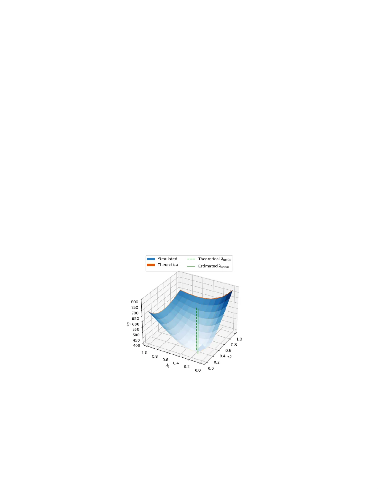
Expectation Err or Bounds f or T ransfer Learning in Linear Regr ession and Linear Neural Networks Meitong Liu M E I T O N G 4 @ I L L I N O I S . E D U University of Illinois Urbana-Champaign Christopher Jung C H R I S J U N G @ M E T A . C O M Meta Rui Li RU I L I 2 3 @ M E TA . C O M Meta Xue F eng X U E F E N G . C S @ G M A I L . C O M Meta Han Zhao H A N Z H AO @ I L L I N O I S . E D U University of Illinois Urbana-Champaign Abstract In transfer learning, the learner lev erages auxiliary data to improv e generalization on a main task. Howe v er , the precise theoretical understanding of when and how auxiliary data help remains in- complete. W e provide new insights on this issue in two canonical linear settings: ordinary least squares regression and under-parameterized linear neural networks. For linear regression, we de- riv e exact closed-form expressions for the e xpected generalization error with bias-v ariance decom- position, yielding necessary and sufficient conditions for auxiliary tasks to improve generalization on the main task. W e also deriv e globally optimal task weights as outputs of solvable optimization programs, with consistency guarantees for empirical estimates. For linear neural networks with shared representations of width q ≤ K , where K is the number of auxiliary tasks, we deri ve a non- asymptotic expectation bound on the generalization error, yielding the first non-vacuous sufficient condition for beneficial auxiliary learning in this setting, as well as principled directions for task weight curation. W e achiev e this by proving a new column-wise low-rank perturbation bound for random matrices, which improves upon existing bounds by preserving fine-grained column struc- tures. Our results are verified on synthetic data simulated with controlled parameters. Keyw ords: Transfer learning, Multi-task learning, Auxiliary data, Linear regression, Linear neural networks, Lo w-rank approximation, Bias-variance trade-of f 1. Intr oduction T ransfer learning, which aims to improve performance in a target domain by transferring kno wledge from a source domain, has been a critical topic in machine learning ( Pan and Y ang , 2009 ; K ouw and Loog , 2018 ; Zhuang et al. , 2020 ). In a similar spirit, multi-task learning (MTL) aims to boost generalization across multiple tasks by pooling shared information through joint training ( Caruana , 1997 ; Ruder , 2017 ; Zhang and Y ang , 2021 ). While MTL is usually ev aluated by an aggregation of task objecti ves, such as the weighted av erage, it is essential to examine whether each task actually benefits from the information transfer . Specifically , viewing a task of interest as the main task and others as the auxiliary , is the jointly trained model better on the main task than a model trained without auxiliary data? In this work, we present ne w theoretical results on this question. © M. Liu, C. Jung, R. Li, X. Feng & H. Zhao. L I U J U N G L I F E N G Z H AO Formally , giv en a training set D = ( X , Y m , { Y k } K k =1 ) , where X is the shared feature, Y m , Y 1 ∼ K are the main and auxiliary labels, an estimator ˆ w D is learned with auxiliary tasks weighted by { λ k } K k =1 . Our goal is to characterize the expected generalization error of ˆ w D on the main task: E K := E D, ( x,y m ) h ( x ⊤ ˆ w D − y m ) 2 i , where ( x, y m ) is a test point drawn from the main task distrib ution. This enables us to inv estigate the follo wing questions: (1) What are the factors that influence E K , and how? (2) When do auxiliary data help, i.e, E K < E 0 , where E 0 is the error when no auxiliary data are in volved? and (3) How to select the task weights { λ k } K k =1 to minimize E K ? W e focus on two canonical linear frame works for learning ˆ w D : (1) ordinary least squares regres- sion and (2) linear neural networks with a shared representation layer of width q and task-specific output heads. Even in these simple setups, existing results for the abov e questions remain incom- plete. Prior work on linear regression often limits its analyses to K = 1 auxiliary source, nor have they de veloped practical methods for selecting optimal task weights ( Dhifallah and Lu , 2021 ; Dar and Baraniuk , 2022 ). Linear neural networks with width q < K + 1 pose fundamental challenges due to a random lo w-rank truncation in the learned estimator, leaving non-asymptotic modeling of E K an open problem ( W u et al. , 2020 ; Y ang et al. , 2025 ). In this work, we fill in these gaps with exact or upper bounds for E K , featuring the first theoretical analysis for optimal weight selection in linear regression and the first non-v acuous suf ficient condition for beneficial auxiliary learning in under-parameterized linear networks, along with other insights. T echnically , we also contribute to the study of random matrix theory with a ne w column-wise lo w-rank perturbation bound. 1.1. Our Contributions Linear regr ession Our technical results can be summarized as follo ws: • W e deri ve exact e xpressions for E K with bias-v ariance decomposition (Theorem 4 ), formalizing the trade-of f mechanism that auxiliary data increases bias but potentially decreases v ariance. • W e obtain necessary and sufficient conditions for beneficial auxiliary learning as an upper bound on the total weight of auxiliary tasks (Corollary 5 ), which translates to a call for higher task similarity , smaller composite auxiliary noise, and moderate sample size for positiv e transfer . • W e solve for the optimal task weights that minimize E K via a con vex quadratic program o ver the simplex and a closed-form formula (Theorem 6 ). Based on empirical estimates for the true solu- tions, we develop a practical method for weight tuning with consistency guarantees (Theorem 7 ), of fering the first weight optimization strategy for transfer learning in linear re gression. Linear neural networks W e focus on the under-parameterized case where the netw ork width q < K + 1 , as otherwise the model capacity is too large for any information transfer ( W u et al. , 2020 ). In this case, the central difficulty arises from the highly nonlinear lo w-rank approximation of a random matrix in the learned estimator , rendering an exact characterization of E K intractable. W e instead pursue an upper bound U ( E K ) with the critical requirement that it can be less than E 0 , so that we obtain useful information by setting U ( E K ) < E 0 . By proving a ne w column-wise low-rank perturbation bound and careful concentration of random matrices, we deri ve such a U ( E K ) : Theorem 1 (informal; see Theorem 8 ) Let N be the number of samples and d be the featur e di- mension with N > d + 3 . Define the weight matrix Λ = diag( { √ λ k } K k =1 ∪ { 1 } ) and the task matrix 2 E X P E C T A T I O N E R RO R B O U N D S F O R T R A N S F E R L E A R N I N G I N L I N E A R R E G R E S S I O N A N D L I N E A R N N S T able 1: Comparison of low-rank perturbation bounds. Here, δ q ( S ) = σ q ( S ) − σ q +1 ( S ) , r = δ q ( S ) / ∥ Z ∥ , and P U = U : ,q U ⊤ : ,q , where U : ,q contains the top q left singular vectors of S . Source Object Assumption Bound Possible to be smaller than ∥ Z ∥ or ∥ Z e j ∥ ? EYM ( T ran et al. , 2025 ) ∥ [ M ] q − [ S ] q ∥ - 2( σ q +1 ( S ) + ∥ Z ∥ ) No TVV ( T ran et al. , 2025 ) ∥ [ M ] q − [ S ] q ∥ r ≥ 4 6 r r − 2 ∥ Z ∥ ( σ q ( S ) δ q ( S ) + log 6 σ 1 ( S ) δ q ( S ) ) No Ours (Theorem 9 ) ∥ ([ M ] q − [ S ] q ) e j ∥ r > 1 1 r − 1 ( ∥ S e j ∥ + ∥ Z e j ∥ ) + ∥ P U Z e j ∥ Y es W ∗ = [ w ∗ 1 , . . . , w ∗ K , w ∗ m ] , wher e w ∗ m (r esp. w ∗ k ) is the true model for the main task (r esp. the k -th auxiliary task). Given that a signal-to-noise ratio r tunable by task weights satisfy r > 1 , we have E K ≤ O (1) σ 2 q +1 ( W ∗ Λ) + O (1)  ∥ w ∗ m ∥ r − 1  2 + O  1 N   d ( r − 1) 2 + q  =: U ( E K ) , wher e O ( · ) r eflects the or ders of N and d , and σ q +1 ( · ) denotes the ( q + 1) -th lar gest singular value . Our bound reveals two driving factors: lo w-rank truncation loss as σ q +1 ( W ∗ Λ) and a tunable signal-to-noise ratio r . Crucially , by curating task weights to reduce σ q +1 ( W ∗ Λ) and increase r , we can hav e E K < U ( E K ) < E 0 . This establishes the first non-vacuous sufficient condition for beneficial auxiliary learning in this setting. By the interaction between Λ and other parameters in r and σ q +1 ( W ∗ Λ) , the bound also provides principled suggestions on weight selection. The proof of U ( E K ) relies on our ne w column-wise lo w-rank perturbation bound (Theorem 9 ). Gi ven a signal matrix S and a subGaussian perturbation Z , with M = S + Z , we aim to bound ∥ ([ M ] q − [ S ] q ) e j ∥ , where e j is the j -th standard basis. In order to hav e U ( E K ) < E 0 , the bound must not be tri vially larger than the original column perturbation ∥ Z e j ∥ . Howe ver , naiv ely relaxing ∥ ([ M ] q − [ S ] q ) e j ∥ ≤ ∥ [ M ] q − [ S ] q ∥ and applying state-of-the-art results ( T ran et al. , 2025 ) fails to achie ve this: as in T able 1 , the coef ficients for ∥ Z ∥ in these bounds are always larger than one. In contrast, our bound remains nontri vial: as it can be proven that ∥ P U Z e j ∥ is asymptotically smaller than ∥ Z e j ∥ , with a suf ficiently large r , the bound improves upon ∥ Z e j ∥ . This is achie ved by preserving the fine-grained column information e j , instead of coarsening to the full error . 1.2. Related W ork Our work contributes to the theoretical understanding of transfer learning. Early work in domain adaptation explored generalization bounds in terms of v arious network complexity measures ( Cram- mer et al. , 2008 ; Mansour et al. , 2009 ; Ben-Da vid et al. , 2010 ), which are often too loose to account for the positi ve and negati ve transfers. Hanneke and Kpotufe ( 2019 ); Mousavi Kalan et al. ( 2020 ) established minimax lower bounds to quantify the limit of how much benefit auxiliary data can pro- vide. By contrast, our goal is to study the precise error for specific model classes and algorithms. In the context of linear regression, Dhifallah and Lu ( 2021 ) conducted an asymptotic analysis of the target test error , where the sample size N and feature dimension d approach infinity under a fixed ratio. Y ang et al. ( 2025 ) further studied different distribution shifts between the source and target in this setting. Dar and Baraniuk ( 2022 ); Ju et al. ( 2023 ) studied the non-asymptotic beha vior of ov er-parameterized regressors, where a subset of parameters can be re-trained on the target. On this line, we contribute our non-asymptotic analysis of E K that applies to multiple tasks rather than two as in most pre vious work, and the first theoretical analysis for optimizing E K ov er task weights. 3 L I U J U N G L I F E N G Z H AO Studies on linear neural networks remain limited. W u et al. ( 2020 ) first examined the archi- tecture employed in this work, rev ealing the necessity of restricting model width for information transfer . In the under-parameterized case, they bound the relativ e distance between the fitted and true estimators, which, howe ver , does not indicate whether incorporating auxiliary data is benefi- cial. More related, Y ang et al. ( 2025 ) derived an asymptotic limit of the main task generalization error , from which our bound in Theorem 8 differs in two ways. First, their analysis operates in the asymptotic setting, while ours applies to finite N and d . Second, gi ven the limiting scenario, their proof relies on high-probability ev ents without tail specification. In contrast, we provide an expectation bound that accounts for the full distribution. Giv en such distinctions, the tw o results are generally incomparable and of fer dif ferent perspectives on this rarely studied setting. For the lo w-rank perturbation, apart from the results in T able 1 , Mangoubi and V ishnoi ( 2022 , 2025 ) bounded the Frobenius norm ∥ [ M ] q − [ S ] q ∥ F , which are looser by nature and do not apply to our context. T o our best knowledge, no w ork has addressed the column-specific error . 2. Problem Setup and Preliminaries Notation. Gi ven a positive integer n , we use [ n ] for the set { 1 , 2 , . . . , n } . W e use ∥ · ∥ for the vector ℓ 2 norm and the matrix spectral norm, and use ∥ · ∥ F for the matrix Frobenius norm. W e use e j to denote the standard basis vector with 1 on the j -th entry and 0 elsewhere. Gi ven random v ariables X and Y , E X [ X Y ] is the expectation o ver X . Data. W e consider re gression problems with one main task and K ≥ 1 auxiliary tasks. A training set is gi ven as D = ( X , Y m , Y 1 , . . . , Y K ) , where X ∈ R N × d is the shared feature with full column rank, Y m ∈ R N is the main task labels, and Y k ∈ R N , k ∈ [ K ] are the auxiliary labels. W e assume the number of samples N and the feature dimension d satisfy N > d + 1 ; for linear NNs, we ask for N > d + 3 . W e also assume K + 1 ≪ d , which holds in most real-world low-dimension scenarios. W e consider linear data modeling: for any task t ∈ [ K ] ∪ { m } , labels are generated as Y t = X w ∗ t + ϵ t , where w ∗ t ∈ R d is the ground-truth model and ϵ t ∈ R N is the label noise. Follo wing prior works ( W u et al. , 2020 ; Mousavi Kalan et al. , 2020 ), we assume each row of X is dra wn independently from N (0 , Σ x ) , where Σ x ∈ R d × d is the cov ariance matrix. W e assume ∥ Σ x ∥ = 1 and σ min (Σ x ) > 0 . Each entry of ϵ t is drawn independently from N (0 , σ 2 t ) . Linear regression. For the first part of this work, we learn a shared estimator ˆ w D ∈ R d that predicts ˆ Y = X ˆ w D for all tasks and minimizes a weighted sum of MSE losses: ˆ w D = arg min w ∈ R d ∥ X w − Y m ∥ 2 + K X k =1 λ k ∥ X w − Y k ∥ 2 , (1) where λ k ≥ 0 for all k ∈ [ K ] are the task weights. When the main task is weighted by λ m ≥ 0 and λ m + P K k =1 λ k = 1 , this is the linear scalarization technique in multi-task learning ( Caruana , 1997 ). In this work, we fix λ m = 1 and only require non-negati vity for the others. Our results apply to both settings with minor tweaks. Standard analysis solves Equation ( 1 ): ˆ w D = 1 1 + P K k =1 λ k ( X ⊤ X ) − 1 X ⊤ Y m + K X k =1 λ k ( X ⊤ X ) − 1 X ⊤ Y k ! , (2) which is a con vex combination of the ordinary least squares (OLS) estimators for each task. 4 E X P E C T A T I O N E R RO R B O U N D S F O R T R A N S F E R L E A R N I N G I N L I N E A R R E G R E S S I O N A N D L I N E A R N N S Linear neural networks. W ithout loss of generality , we consider two-layer neural networks with a shared layer B ∈ R d × q and task-specific heads a m ∈ R q , a k ∈ R q , k ∈ [ K ] . The prediction for the main task (resp. the k -th auxiliary task) is ˆ Y m = X B a m (resp. ˆ Y k = X B a k ). An y deeper linear network can be reduced to this structure of a shared encoder and separate heads. W e adopt a weighted MSE loss similar to Equation ( 1 ). Define A = [ a 1 , . . . , a K , a m ] , Λ = diag( { √ λ k } K k =1 ∪ { 1 } ) , and Y = [ Y 1 , . . . , Y K , Y m ] , the objectiv e can be written as ˆ B D , ˆ A D = arg min B ,A ∥ ( X B A − Y )Λ ∥ 2 F . Denoting ˆ w m = ˆ B D ˆ a m and ˆ w k = ˆ B D ˆ a k , k ∈ [ K ] as the composite estimators for each task and their stack ˆ W D = [ ˆ w 1 , . . . , ˆ w K , ˆ w m ] , we can re write the model as ˆ W D = arg min W ∈ R d × ( K +1) , rank( W ) ≤ q ∥ ( X W − Y )Λ ∥ 2 F . (3) There are two regimes based on the width of the shared layer , q . When q ≥ K + 1 , we are in the ov er-parameterized case, where we hav e the following result: Proposition 2 (restated from W u et al. ( 2020 )) When q ≥ K + 1 , any optimal solution ˆ W D to Equation ( 3 ) satisfies ˆ w m = ( X ⊤ X ) − 1 X ⊤ Y m , ˆ w k = ( X ⊤ X ) − 1 X ⊤ Y k , k ∈ [ K ] . In other words, when the model is large enough, the optimal composite estimator for each task is its OLS estimator, which is equiv alent to learning each task indi vidually . This leads to the conclusion in W u et al. ( 2020 ) that limiting model capacity is necessary for information transfer . Consequently , we focus on the under-parameterized case with q < K + 1 . Proposition 3 (restated from Hu et al. ( 2023 )) When q < K + 1 , Equation ( 3 ) gives ˆ W D = X † [ P X Y Λ] q Λ − 1 , (4) wher e P X = X ( X ⊤ X ) − 1 X ⊤ is the pr ojection matrix that maps to the column space of X . The optimal composite estimator for each task is then ˆ w m = ˆ W D e K +1 , ˆ w k = ˆ W D e k , k ∈ [ K ] . Here, [ · ] q denotes the best rank- q approximation of a matrix under an y unitarily in variant norm. For a matrix A ∈ R m × n with SVD A = P min( m,n ) i =1 σ i u i v ⊤ i , where σ 1 ≥ . . . ≥ σ min( m,n ) , by the Eckart-Y oung-Mirsky Theorem ( Eckart and Y oung , 1936 ), we ha ve [ A ] q = P q i =1 σ i ( A ) u i v ⊤ i . Learning goal. Giv en the empirical risk minimizers for the two settings defined in Equations ( 1 ) and ( 3 ), we aim for a smaller expected generalization error on the main task, namely E := E D, ( x,y m ) h ( x ⊤ ˆ w m − y m ) 2 i , (5) where D denotes the training set and ( x, y m ) is freshly sampled from the main task distribution: draw x ∼ N (0 , Σ x ) , ϵ ∼ N (0 , σ 2 m ) , and set y m = x ⊤ w ∗ m + ϵ . Note that ˆ w m ( ˆ w D in linear regression) is a function of the random training set D . 5 L I U J U N G L I F E N G Z H AO 3. A uxiliary Data in Linear Regression In this section, we study when and how auxiliary data improv e generalization on the main task in linear regression. In Section 3.1 , we obtain the exact expected generalization errors, showing that auxiliary learning can be understood as a bias-v ariance trade-of f. In Section 3.2 , we deriv e the necessary and sufficient conditions for beneficial incorporation and the optimal task weights. These results formalize the interaction between task weights, task similarity , noise le vels, and sample size, and of fer a practical method for weight selection with good statistical properties. 3.1. From the V iew of Bias-V ariance T rade-off Starting from Equation ( 5 ), we first apply the bias-variance decomposition. This step is not a must, but it helps interpret the ef fect of considering auxiliary tasks. Specifically , we have E = E D, ( x,y m ) h ( x ⊤ ˆ w D − y m ) 2 i = E D,x h ( x ⊤ ( ˆ w D − ¯ w )) 2 i | {z } variance + E x h ( x ⊤ ( ¯ w − w ∗ m )) 2 i | {z } bias + σ 2 m |{z} noise where ¯ w = E D [ ˆ w D ] is the expected estimator . Conceptually , v ariance arises from the randomness of a finite training set. As the sample size gro ws to infinity , it vanishes to 0. Bias is determined by the learning algorithm and the capacity of the hypothesis class. It does not scale with the sample size. The noise term is E ( x,y m ) [( x ⊤ w ∗ m − y m ) 2 ] = E ϵ [ ϵ 2 ] , which comes from the label noise. Follo wing this framew ork, we obtain the exact form of the expected generalization error: Theorem 4 Let E K be the expected main task generalization err or when K auxiliary tasks ar e included. Suppose the auxiliary tasks ar e weighted by { λ k } K k =1 , then we have E K = σ 2 m + P K k =1 λ 2 k σ 2 k (1 + Λ) 2 d N − d − 1 | {z } variance +  Λ 1 + Λ  2 ∥ Σ 1 2 x ( w ∗ aux − w ∗ m ) ∥ 2 | {z } bias + σ 2 m |{z} noise , (6) wher e Λ = P K k =1 λ k > 0 and w ∗ aux = 1 Λ P K k =1 λ k w ∗ k . In particular , when K = 0 or Λ = 0 , the expected g eneralization err or of learning the main task only is E 0 = σ 2 m d N − d − 1 | {z } variance + 0 |{z} bias + σ 2 m |{z} noise . (7) Proof sketch The bias follo ws from computing ¯ w from Equation ( 2 ). The variance follows from the trace-expectation identity and the mean of an in verse-W ishart distribution. See Section A.1 . From the decompositions of E 0 and E K , it is clear that bringing in auxiliary information in- creases bias due to their difference from the main task. Indeed, the bias term in E K e v aluates a weighted distance between w ∗ aux and w ∗ m . On the other hand, variance can be reduced giv en proper weights and auxiliary label noise. For example, when σ 2 k = σ 2 m and λ k = 1 for all k ∈ [ K ] , the noise coefficient is reduced by a factor of K + 1 . Therefore, to benefit from the auxiliary data, one must ensure that the decrease in v ariance outweighs the increase in bias. 6 E X P E C T A T I O N E R RO R B O U N D S F O R T R A N S F E R L E A R N I N G I N L I N E A R R E G R E S S I O N A N D L I N E A R N N S 3.2. Utility Conditions and Optimal W eighting Gi ven Theorem 4 , we obtain the necessary and sufficient conditions for auxiliary tasks to help, i.e., E K < E 0 , as well as the optimal task weights that minimize E K . W e first introduce a necessary re-parameterization. When K > 1 , directly optimizing Equa- tion ( 6 ) ov er { λ k } yields a noncon ve x fractional quadratic program, which admits no closed-form solution or solver with global optimality guarantees. T o resolve this, we re-parameterize { λ k } : let Λ = P K k =1 λ k > 0 , and for any k ∈ [ K ] , let λ ′ k = λ k / Λ , such that P K k =1 λ ′ k = 1 , i.e., λ ′ = [ λ ′ 1 , . . . , λ ′ K ] ∈ ∆ K , where ∆ K denotes the ( K − 1) -dimensional simplex. Here, Λ controls the ov erall scale of the auxiliary tasks, and { λ ′ k } controls their proportion. The optimal values are then solv able. W e thus present results in this subsection using the ne w parameterization. The follo wing corollary provides the necessary and suf ficient conditions for beneficial auxiliary learning. It is a direct result of setting E K < E 0 using Theorem 4 and some reorg anization. Corollary 5 Suppose the auxiliary tasks ar e weighted by { λ k } K k =1 , then E K < E 0 iff . ( K X k =1 ( λ ′ k ) 2 σ 2 k − σ 2 m ) d N − d − 1 + ∥ Σ 1 2 x ( w ∗ aux − w ∗ m ) ∥ 2 ! | {z } L Λ < 2 σ 2 m d N − d − 1 | {z } R , (8) wher e Λ = P K k =1 λ k , λ ′ k = λ k / Λ , k ∈ [ K ] , and w ∗ aux = 1 Λ P K k =1 λ k w ∗ k = P K k =1 λ ′ k w ∗ k . Remark Recall that Λ denotes the total strength of the auxiliary tasks. Hence, by Equation ( 8 ), for a meaningful incorporation, L should be either (1) negati ve, and any weight combination with Λ > 0 suffices, or (2) positi ve but small, so that after dividing it on both sides, the resulting upper limit on Λ , i.e., Λ < R L is not tri vially tiny . This translates to the needs of se veral factors: • Higher task similarity in terms of a smaller distance term, ∥ Σ 1 2 x ( w ∗ aux − w ∗ m ) ∥ . • Smaller composite auxiliary label noise , P K k =1 ( λ ′ k ) 2 σ 2 k . • Moderate sample size : W ith a fixed d , as N gro ws to infinity , the LHS coefficient becomes positi ve, while the RHS vanishes, which forces Λ to be near 0. Hence, for auxiliary data to be influential, the shared samples should not be “too sufficient”. Otherwise, as discussed in Section 3.1 , there is not much v ariance to be traded with bias. In addition to the inherent task structures, one can also tune λ ′ to optimize these f actors. In fact, the optimal weights are solv able after the re-parameterization. Theorem 6 F or any α ∈ ∆ K , define f ( α ) = d N − d − 1 P K k =1 ( α k ) 2 σ 2 k + δ ( α ) ⊤ Σ x δ ( α ) , wher e δ ( α ) = P K k =1 α k w ∗ k − w ∗ m . The optimal weights that minimize E K as in Equation ( 6 ) ar e λ ′∗ = arg min α ∈ ∆ K f ( α ) , Λ ∗ = σ 2 m d N − d − 1 · 1 f ( λ ′∗ ) , (9) and we reco ver λ ∗ k = Λ ∗ λ ′∗ k , k ∈ [ K ] . Optimizing f ( α ) is a con vex quadratic pr ogram over the simplex, whic h can be solved by off-the-shelf methods. When K = 1 , we have λ ′∗ = 1 , λ ∗ = Λ ∗ . 7 L I U J U N G L I F E N G Z H AO Proof By Equation ( 6 ), minimizing E K is equi valent to minimizing c +Λ 2 f ( λ ′ ) (1+Λ) 2 , where c is a con- stant. Optimizations for Λ and λ ′ can then be disentangled: for λ ′ , it reduces to minimizing f ( λ ′ ) ; for a fixed λ ′ , the optimal Λ ∗ is obtained by the first- and second-order optimality conditions. Based on Theorem 6 , we pro vide guidance on selecting task weights giv en a training set in prac- tice, where the distribution parameters are unknown. As a standard approach, we replace unknowns with data-deriv ed estimators and solve for the estimated optimal weights, denoted as ˆ λ ∗ . Let us then consider its statistical properties. Since E K contains an interaction term between w ∗ and Σ x , it is dif ficult to ensure unbiasedness. Optimizing an unbiased estimator for E K also does not guarantee an unbiased estimator for the true optimal weights. Nev ertheless, ˆ λ ∗ prov es to be consistent: Theorem 7 Given a training set D = ( X , Y m , Y 1 , . . . , Y k ) , for t ∈ [ K ] ∪ { m } , we have ˆ w t = ( X ⊤ X ) − 1 X ⊤ Y t p → w ∗ t , ˆ σ 2 t = ∥ Y t − X ˆ w t ∥ 2 N − d p → σ 2 t , and ˆ Σ x = 1 N X ⊤ X p → Σ x . Let ˆ λ be the solution to Equation ( 9 ) after plugging in these consistent estimators, and λ ∗ = arg min λ E K be the true optimal weights. If a unique λ ∗ exists, and ∃ B < ∞ such that ∥ λ ∗ ∥ ≤ B , ∥ ˆ λ ∥ ≤ B , then ˆ λ p → λ ∗ . Proof sketch This follo ws from the consistency of M-estimators. See Section A.2 . Since the gi ven consistent estimators are asymptotically Gaussian, one can also approximate the v ariance and confidence intervals for ˆ λ by its asymptotic normality , which can be justified via either the delta method ( Cram ´ er , 1999 ) or the properties of M-estimators ( V an der V aart , 2000 ). Con ventionally , tuning task weights requires a grid search o ver a held-out set. For lar ge K , this can be computationally and statistically expensi ve. Our theoretical analysis and practical solution of fer a way to identify a prov ably good candidate, near which a small-scale grid search can be conducted for finer tuning. Finally , we note that although the above method is based on a gi ven D , it does not aim to minimize the error for this specific set. Instead, by the definition in Equation ( 5 ), we aim to be optimal in expectation o ver randomly drawn sets. 4. A uxiliary Data in Under -Parameterized Linear Networks Next, we study the setting of under -parameterized linear neural networks. In Section 4.1 , we present the expectation bound for the main task generalization error, integrating task weights, task struc- tures, model capacity , and a tunable signal-to-noise ratio. The bound is informative in the sense of yielding a non-vacuous suf ficient condition for beneficial auxiliary learning. W e also introduce our column-wise lo w-rank perturbation bound, which possesses key potential not achieved by existing results to improv e upon the original perturbation. W e then walk through the proofs in Section 4.2 . 4.1. An Inf ormative Expectation Bound on the Generalization Error by a New Column-Wise Low-Rank Perturbation Bound T o compute the expected generalization error, one has to consider the random beha vior of the learned estimator ˆ w m . By Proposition 3 , the solution to this setting consists of a low-rank ap- proximation of a random matrix, [ P X Y Λ] q , whose exact expectation is generally hard to deri ve due to the highly nonlinear SVD operation. Hence, we aim for an upper bound. 8 E X P E C T A T I O N E R RO R B O U N D S F O R T R A N S F E R L E A R N I N G I N L I N E A R R E G R E S S I O N A N D L I N E A R N N S Theorem 8 Let E K denote the expected main task generalization err or when K auxiliary tasks ar e included with weights { λ k } K k =1 via a linear network with width q < K + 1 . Define Λ = diag( { √ λ k } K k =1 ∪ { 1 } ) , W ∗ = [ w ∗ 1 , . . . , w ∗ K , w ∗ m ] , ϵ = [ ϵ 1 , . . . , ϵ K , ϵ m ] , where ϵ t = Y t − X w ∗ t , ∀ t ∈ [ K ] ∪ { m } , and P X = X ( X ⊤ X ) − 1 X ⊤ . If σ q ( X W ∗ Λ) − σ q +1 ( X W ∗ Λ) ∥ P X ϵ Λ ∥ ≥ r > 1 , ∀ X , ∀ ϵ , we have E K ≤ 2 C 4 κ (Σ x ) √ N + √ d √ N − d +3 √ N ! 2 σ 2 q +1 ( W ∗ Λ) | {z } T 1 + 6 C 4 κ (Σ x ) √ N + √ d √ N − d +3 √ N ! 2  ∥ w ∗ m ∥ r − 1  2 | {z } T 2 + 6 σ 2 m C 3 σ min (Σ x ) 1 √ N − d +1 √ N ! 2  C 1 d ( r − 1) 2 + C 2 q  | {z } T 3 + σ 2 m =: U ( E K ) , wher e σ q ( · ) is the q -th lar gest singular value, κ ( · ) is the condition number , and C 1 ∼ 4 ar e constants. Remark Let us comment on the theorem. First, the condition on r characterizes a strength ratio of noise-free label information to label noise. In other words, r serves as a lower bound of the signal- to-noise ratio , rendering r > 1 a reasonable requirement. Next, one sees that U ( E K ) decreases with (1) a smaller σ q +1 ( W ∗ Λ) in T 1 , which reflects ho w much information is left out by the low- rank truncation, and (2) naturally , a larger r , which reduces T 2 and T 3 . These values integrate the ef fects of task weights Λ , model capacity q , how aligned tasks are, and their noise lev els. Gi ven a fixed q , the bound suggests tuning Λ to amplify high-quality auxiliary tasks that align with the main and suppress distinct, noisy ones, as this leads to a clustered spectrum with a larger spectral gap, a smaller composite noise, and, therefore, (1) less truncation loss and (2) a larger r . Still, our goal is to reveal when auxiliary data help. With q ≥ 1 , learning the main task alone gi ves ˆ w m = ( X ⊤ X ) − 1 X ⊤ Y m . Hence, E 0 is the same as in Equation ( 7 ). By setting U ( E K ) < E 0 , one obtains a sufficient condition for E K < E 0 . Howe ver , the validity of such a condition relies on a critical question: Is U ( E K ) possible to be smaller than E 0 by tuning the task weights? If not, the bound may be too loose to provide useful information. Our answer is affirmati ve. Comparing T 3 with the variance of E 0 , σ 2 m d N − d − 1 , both are of order O ( d/ N ) given that q < K + 1 ≪ d . If r is large, the coefficient of d in T 3 can be significantly reduced, making T 3 smaller than the E 0 v ariance. When such a reduction outweighs the increase from T 1 and T 2 , which can also be minimized with a larger r and a smaller truncation loss, we ha ve U ( E K ) < E 0 . By form, one can view T 1 and T 2 as the bias of order O (1) , and T 3 as the variance of order O (1 / N ) . Then, the condition coincides with the bias-variance trade-of f rule. In the proof of Theorem 8 , one ke y step is to bound a column-wise lo w-rank perturbation: ∥ ([ M ] q − [ S ] q ) e j ∥ , where M = S + Z and Z is a Gaussian random matrix. T o mak e U ( E K ) < E 0 possible, the bound must not be trivially larger than the original perturbation ∥ Z e j ∥ . Unfortunately , existing state-of-the-art tools cannot achiev e this goal ( T ran et al. , 2025 ). W e hence develop the follo wing theorem, which preserves fine-grained column structures and harnesses a similar signal- to-noise ratio as in Theorem 8 . This result might also be of independent interest to future work. 9 L I U J U N G L I F E N G Z H AO Theorem 9 F or any matrix S, Z ∈ R m × n , let M = S + Z . When σ q ( S ) − σ q +1 ( S ) ∥ Z ∥ ≥ r > 1 , we have, for any q ∈ [rank( S )] and j ∈ [ n ] , ∥ ([ M ] q − [ S ] q ) e j ∥ ≤ 1 r − 1 ( ∥ S e j ∥ + ∥ Z e j ∥ ) + ∥ P U Z e j ∥ =: U q ,j , wher e P U is the pr ojection matrix that maps onto the subspace spanned by the first q left singular vectors of S , i.e., with SVD S = U Σ V ⊤ , we have P U = U : ,q U ⊤ : ,q . T o see how U q ,j can be smaller than ∥ Z e j ∥ , we first argue that ∥ P U Z e j ∥ < ∥ Z e j ∥ asymptoti- cally when Z e j is mean-zero subgaussian as in our context: due to the rank- q projection, ∥ P U Z e j ∥ is of order O ( √ q ) , while ∥ Z e j ∥ is of order O ( √ m ) . Then, when r is large and ∥ S e j ∥ is small, we can hav e U q ,j < ∥ Z e j ∥ . W e defer the proof and elaboration to Section 4.2.1 . 4.2. Proof of Theorem 8 The proof of Theorem 8 proceeds in two main steps: (1) bounding the column-wise low-rank per- turbation (Section 4.2.1 ) and (2) bounding expectations of random matrices (Section 4.2.2 ). W e first introduce three key matrices M , S, Z . W e use e m for e K +1 , as the ( K + 1) -th column holds the main task values. Let M = P X Y Λ ; by Equation ( 4 ), we hav e ˆ w m = X † [ M ] q Λ − 1 e m = X † [ M ] q e m , where the second step comes from the last entry of Λ being 1 . Let S = P X X W ∗ Λ = X W ∗ Λ be the pure signal, and Z = P X ϵ Λ be the projected noise. W ith Y = X W ∗ + ϵ , we have M = S + Z . Finally , by the definition of S , we have w ∗ m = X † S Λ − 1 e m = X † S e m . The proof starts from the definition in Equation ( 5 ). First, one sees that bounding E K boils do wn to bounding E D ∥ ˆ w m − w ∗ m ∥ 2 . Specifically , with y m = x ⊤ w ∗ m + ϵ m , we hav e E K = E D, ( x,y m ) [( x ⊤ ˆ w m − y m ) 2 ] = E D,x [( x ⊤ ( ˆ w m − w ∗ m )) 2 ] + σ 2 m . Let ∆ = ˆ w m − w ∗ m ; we hav e E D,x h ( x ⊤ ∆) 2 i = E D h ∆ ⊤ E x [ xx ⊤ ]∆ i = E D [∆ ⊤ Σ x ∆] ≤ ∥ Σ x ∥ · E D ∥ ∆ ∥ 2 = E D ∥ ∆ ∥ 2 (10) where the inequality follows from | ∆ ⊤ Σ x ∆ | ≤ ∥ ∆ ∥ · ∥ Σ x ∥ · ∥ ∆ ∥ . Next, we plug in ˆ w m = X † [ M ] q e m and w ∗ m = X † S e m deri ved above and perform an add-and-subtract operation with [ S ] q : E D ∥ ˆ w m − w ∗ m ∥ 2 = E D ∥ X † ([ M ] q − [ S ] q + [ S ] q − S ) e m ∥ 2 ≤ E D h ∥ X † ∥ 2  2 ∥ ([ M ] q − [ S ] q ) e m ∥ 2 + 2 ∥ ([ S ] q − S ) e m ∥ 2  i . (11) For the second term, one has ∥ ([ S ] q − S ) e m ∥ ≤ ∥ [ S ] q − S ∥∥ e m ∥ = σ q +1 ( S ) by the Eckart-Y oung- Mirsky (EYM) Theorem ( Eckart and Y oung , 1936 ). W e are then left with ∥ ([ M ] q − [ S ] q ) e m ∥ . 4 . 2 . 1 . B O U N D I N G T H E C O L U M N - W I S E L O W - R A N K P E RT U R B A T I O N W e first illustrate why a useful bound U q ,m for ∥ ([ M ] q − [ S ] q ) e m ∥ should not always be larger than ∥ Z e m ∥ . Consider the competitor E 0 ; by the same deriv ation for Equation ( 10 ), we hav e E 0 = E D ∥ ∆ 0 ∥ 2 + σ 2 m , where ∆ 0 = ˆ w m − w ∗ m = ( X ⊤ X ) − 1 X ⊤ ( Y − X w ∗ m ) = X † P X ϵ m . Notice that Z e m = P X ϵ Λ e m = P X ϵe m = P X ϵ m . Therefore, proceeding from Equation ( 11 ) with a U q ,m ≥ ∥ Z e m ∥ would lead to an uninformati ve U ( E K ) such that U ( E K ) − σ 2 m ≥ E D h ∥ X † ∥ 2 ∥ Z e m ∥ 2 i ≥ E D ∥ X † P X ϵ m ∥ 2 = E D ∥ ∆ 0 ∥ 2 = E 0 − σ 2 m . 10 E X P E C T A T I O N E R RO R B O U N D S F O R T R A N S F E R L E A R N I N G I N L I N E A R R E G R E S S I O N A N D L I N E A R N N S Thereby , we formalize a more general subproblem: for any matrix S, Z ∈ R m × n , let M = S + Z ; for any q ∈ [rank( S )] and j ∈ [ n ] , find an upper bound for ∥ ([ M ] q − [ S ] q ) e j ∥ that is not alw ays larger than ∥ Z e j ∥ . W e first discuss two existing bounds that fail to satisfy this requirement, follo wed by the proof of our Theorem 9 , which succeeds by preserving fine-grained column information. Attempt 1. By the EYM Theorem and W e yl’ s inequality ( W eyl , 1912 ), a direct bound is ∥ ([ M ] q − [ S ] q ) e j ∥ ≤ ∥ [ M ] q − [ S ] q ∥ · 1 ≤ 2( σ q +1 ( S ) + ∥ Z ∥ ) . W e refer readers to Appendix A of T ran et al. ( 2025 ) for its short proof. Clearly , this bound is always lar ger than ∥ Z ∥ , and thus ∥ Z e j ∥ . Attempt 2. Recently , Tran et al. ( 2025 ) proved a new bound for ∥ [ M ] q − [ S ] q ∥ using a contour bootstrapping method, where S and Z are symmetric. T o apply it to our problem, we extend it to rectangular matrices and align the assumption form with ours: Corollary 10 (Theorem D.1 of T ran et al. ( 2025 )) Given that σ q ( S ) − σ q +1 ( S ) ∥ Z ∥ ≥ r ≥ 4 , we have ∥ [ M ] q − [ S ] q ∥ ≤ 6 r r − 2 ∥ Z ∥ ( σ q ( S ) σ q ( S ) − σ q +1 ( S ) + log 6 σ 1 ( S ) σ q ( S ) − σ q +1 ( S ) ) . The complete proof is in Section B.1 . Since r ≥ 4 and singular values are non-negati ve, the coef ficient of ∥ Z ∥ in this bound is always larger than 1. Hence, using ∥ ([ M ] q − [ S ] q ) e j ∥ ≤ ∥ [ M ] q − [ S ] q ∥ and applying Corollary 10 cannot meet our requirement. Inspired by our final result, we also attempted to inject the column information e j into the proof frame work. Howe ver , due to the form of the contour method, adding e j does not contribute to a potentially smaller coef ficient 1 . Attempt 3. The above unsuccessful attempts essentially aim to address the entire error ∥ [ M ] q − [ S ] q ∥ . They suggest the necessity of considering the role of e j as opposed to discarding it via ∥ e j ∥ = 1 . W ith this in mind, we dev elop Theorem 9 . Proof of Theorem 9 W ith SVD M = ˆ U ˆ Σ ˆ V ⊤ and S = U Σ V ⊤ , define projection matrices ˆ P U = ˆ U : ,q ˆ U ⊤ : ,q and P U = U : ,q U ⊤ : ,q . W e have [ M ] q = ˆ P U M and [ S ] q = P U S . Then, by adding and subtracting P U M e j , follo wed by the triangle inequality , we hav e ∥ ([ M ] q − [ S ] q ) e j ∥ = ∥ ( ˆ P U M − P U S ) e j ∥ ≤ ∥ ( ˆ P U − P U ) M e j ∥ + ∥ P U ( M − S ) e j ∥ ≤ ∥ ˆ P U − P U ∥ ( ∥ S e j ∥ + ∥ Z e j ∥ ) + ∥ P U Z e j ∥ , (12) where the last step follo ws from ∥ ( ˆ P U − P U ) M e j ∥ ≤ ∥ ˆ P U − P U ∥∥ M e j ∥ and M = S + Z . Next, we bound ∥ ˆ P U − P U ∥ by the W edin sin Θ Theorem ( W edin , 1972 ): If σ q ( S ) − σ q +1 ( M ) > 0 , one has ∥ ˆ P U − P U ∥ ≤ ∥ Z ∥ σ q ( S ) − σ q +1 ( M ) . T o unify the singular values, we replace σ q +1 ( M ) with σ q +1 ( M ) ≤ ∥ Z ∥ + σ q +1 ( S ) by W eyl’ s inequality . Hence, the statement translates to: if σ q ( S ) − σ q +1 ( M ) ≥ σ q ( S ) − σ q +1 ( S ) − ∥ Z ∥ > 0 , i.e., σ q ( S ) − σ q +1 ( S ) ∥ Z ∥ ≥ r > 1 , we hav e ∥ ˆ P U − P U ∥ ≤ ∥ Z ∥ σ q ( S ) − σ q +1 ( S ) −∥ Z ∥ ≤ 1 r − 1 . Plugging this into Equation ( 12 ) finishes the proof. The column information e j is preserved throughout this proof. In fact, if ∥ S e j ∥ and ∥ Z e j ∥ in Equation ( 12 ) are coarsened to ∥ S ∥ and ∥ Z ∥ , one will have ∥ S ∥ ≥ σ q ( S ) − σ q +1 ( S ) ≥ r ∥ Z ∥ , which results in a bound with 1 r − 1 ( ∥ S ∥ + ∥ Z ∥ ) ≥ r +1 r − 1 ∥ Z ∥ > ∥ Z ∥ . In contrast, there is no such limitation on ∥ S e j ∥ . It is this key observation of the fine-grained column structure that leads to the superiority of our bound. Finally , we substantiate our previous argument of ∥ P U Z e j ∥ being asymptotically small: 1. There is another contour-based bound in T ran et al. ( 2025 ) (Theorem D.5) that is sometimes tighter than Corollary 10 , but still lar ger than ∥ Z ∥ , and the difficulty of incorporating e j persists. 11 L I U J U N G L I F E N G Z H AO Proposition 11 Let Z e j ∈ R m be a mean-zer o subgaussian random vector with subgaussian norm σ , and P U be the r ank- q pr ojection defined in Theorem 9 . W ith pr obability at least 1 − 2 e − t 2 , we have ∥ Z e j ∥ ≤ C σ ( √ m + t ) and ∥ P U Z e j ∥ ≤ C σ ( √ q + t ) . Alternatively , we have E ∥ Z e j ∥ ≤ C σ √ m and E ∥ P U Z e j ∥ ≤ C σ √ q . Her e, the C ’ s ar e constants. In other words, projecting a random vector onto an independent low-rank subspace largely re- duces its norm. Thereby , ∥ P U Z e j ∥ is nearly negligible when q is small relati ve to m . This completes the claim that our bound can be smaller than ∥ Z e j ∥ when r is large and ∥ P U Z e j ∥ < ∥ Z e j ∥ . The proof of Proposition 11 is deferred to Section B.3 . 4 . 2 . 2 . B O U N D I N G E X P E C TA T I O N S O F R A N D O M M AT R I C E S W e continue with the proof of Theorem 8 . From Equation ( 11 ), we proceed by bounding ∥ ([ M ] q − [ S ] q ) e m ∥ with Theorem 9 , whose condition on r translates to that of Theorem 8 after plugging in the context definitions of S = X W ∗ Λ and Z = P X ϵ Λ . Next, we disentangle the random matrices, i.e., X and Z , from constant v alues. W ith intermediate steps deferred to Section B.2 , we obtain: E K ≤ E X h ∥ X † ∥ 2 ∥ X ∥ 2 i 2 σ 2 q +1 ( W ∗ Λ) + 6  ∥ w ∗ m ∥ r − 1  2 ! + E X h ∥ X † ∥ 2  E ϵ | X ∥ Z e m ∥ 2 + E ϵ | X ∥ P U Z e j ∥ 2  i + σ 2 m . (13) One can see the correspondence between these terms and those in the final bound. It remains to address the expectations. Extending the idea of Proposition 11 , we bound those over Z : Lemma 12 Given the setups in Section 2 , where Z = P X ϵ Λ , we have E ϵ | X ∥ Z e m ∥ 2 ≤ C 1 σ 2 m d and E ϵ | X ∥ P U Z e m ∥ 2 ≤ C 2 σ 2 m q , wher e C 1 and C 2 ar e constants. The proof is provided in Section B.3 . On the outside, we bound those over X : Lemma 13 Given the setups in Section 2 , we have E X ∥ X † ∥ 2 ≤ C 3 σ min (Σ x )  1 √ N − ( d +1) / √ N  2 and E X [ ∥ X † ∥ 2 ∥ X ∥ 2 ] ≤ C 4 κ (Σ x )  √ N + √ d √ N − ( d +3) / √ N  2 , wher e C 3 and C 4 ar e constants. The proof, deferred to Section B.4 , relies on characterizing the smallest singular value of a Gaussian random matrix. Indeed, we have ∥ X † ∥ = 1 /σ min ( X ) . Finally , applying Lemmas 12 and 13 to Equation ( 13 ) finishes the proof of Theorem 8 . 5. Numerical Simulations W e verify our results on synthetic data generated with controlled parameters. Detailed setups are deferred to Appendix C . Figure 1( a ) plots the linear regression setting with one auxiliary task of moderate distance to the main task and a lo wer noise le vel. One sees that the simulated and theoret- ical curves align well. The cleaner auxiliary task helps improv e the main task generalization with small weights, but worsens it beyond a threshold, as its difference from the main task dominates. Computed by Corollary 5 and Theorem 6 , respectiv ely , the theoretical threshold and optimal value for the task weights prove valid, and the plug-in estimators fall in nearby regions. W e also provide 12 E X P E C T A T I O N E R RO R B O U N D S F O R T R A N S F E R L E A R N I N G I N L I N E A R R E G R E S S I O N A N D L I N E A R N N S ( a ) Linear regression with K = 1 . ( b ) Column-wise lo w-rank perturbation bound. ( c ) Generalization bound for linear NN. Figure 1: Simulation results of for both linear regression and linear neural networks. the figure for two auxiliary tasks in Appendix C , where the first program for obtaining the optimal weights in Equation ( 9 ) is solved by projected gradient descent ( Beck , 2017 ). For the linear neural network setting, we first examine our column-wise lo w-rank perturbation bound in Theorem 9 . Figure 1( b ) plots the log-scale errors against the signal-to-noise ratio r . As sho wn, our bound tightly approximates the actual error and can impro ve upon the original perturba- tion when r is large, while the TVV bound from Corollary 10 is much looser due to not preserving column information. Ne xt, Figure 1( c ) sho ws the generalization errors with one auxiliary task and network width q = 1 . Here, the signal-to-noise ratio r is altered with the auxiliary task weight. Computed by Theorem 8 , our bound decreases below E 0 as r grows, when the actual error is indeed better than E 0 . This verifies the non-v acuity and validity of the suf ficient condition. 6. Conclusion In this work, we contribute to the theoretical understanding of transfer learning by studying when and ho w auxiliary data improve generalization on the main task in linear regression and linear neural networks. F or linear regression, we perform exact characterizations of the expected generalization error , yielding the necessary and sufficient condition for beneficial auxiliary learning. W e de velop globally optimal task weights that support the practical computation of consistent empirical estima- tors. For under-parameterized linear networks, we prove a non-asymptotic expectation bound on the generalization error in terms of a weighted signal-to-noise ratio and a tunable lo w-rank truncation loss. W e thereby establish the first non-v acuous sufficient condition for beneficial auxiliary learn- ing in this setting and of fer principled suggestions on weight curation. Our bound builds on a new column-wise lo w-rank perturbation bound, which, unlike e xisting results, preserves the potential to improv e upon the original perturbation by examining column structures. Acknowledgments Meitong Liu is partially supported by an Amazon AI PhD Fellowship. Meitong Liu and Han Zhao are also partially supported by an NSF CAREER A ward No. 2442290. The authors would like to thank Y ifei He, Zhe Kang, Ming Li, and Siqi Zeng for their discussion throughout the dev elopment of this work. 13 L I U J U N G L I F E N G Z H AO References Amir Beck. F irst-or der methods in optimization . SIAM, 2017. Shai Ben-David, John Blitzer , K oby Crammer , Alex K ulesza, Fernando Pereira, and Jennifer W ort- man V aughan. A theory of learning from different domains. Mac hine learning , 79(1):151–175, 2010. Rajendra Bhatia. Matrix analysis , volume 169. Springer Science & Business Media, 2013. Rich Caruana. Multitask learning. Machine learning , 28(1):41–75, 1997. Zizhong Chen and Jack J Dongarra. Condition numbers of gaussian random matrices. SIAM Journal on Matrix Analysis and Applications , 27(3):603–620, 2005. Harald Cram ´ er . Mathematical methods of statistics , v olume 9. Princeton university press, 1999. K oby Crammer , Michael Kearns, and Jennifer W ortman. Learning from multiple sources. 2008. Y ehuda Dar and Richard G Baraniuk. Double double descent: On generalization errors in transfer learning between linear regression tasks. SIAM J ournal on Mathematics of Data Science , 4(4): 1447–1472, 2022. Oussama Dhifallah and Y ue M Lu. Phase transitions in transfer learning for high-dimensional perceptrons. Entr opy , 23(4):400, 2021. Carl Eckart and Gale Y oung. The approximation of one matrix by another of lower rank. Psychome- trika , 1(3):211–218, 1936. Nathan Halko, Per-Gunnar Martinsson, and Joel A T ropp. Finding structure with randomness: Probabilistic algorithms for constructing approximate matrix decompositions. SIAM r eview , 53 (2):217–288, 2011. Ste ve Hanneke and Samory Kpotufe. On the value of target data in transfer learning. Advances in Neural Information Pr ocessing Systems , 32, 2019. Y uzheng Hu, Ruicheng Xian, Qilong W u, Qiuling F an, Lang Y in, and Han Zhao. Revisiting scalar - ization in multi-task learning: A theoretical perspectiv e. Advances in Neural Information Pr o- cessing Systems , 36:48510–48533, 2023. Peizhong Ju, Sen Lin, Mark S Squillante, Y ingbin Liang, and Ness B Shroff. Generalization perfor - mance of transfer learning: Overparameterized and underparameterized regimes. arXiv pr eprint arXiv:2306.04901 , 2023. W outer M Kouw and Marco Loog. An introduction to domain adaptation and transfer learning. arXiv pr eprint arXiv:1812.11806 , 2018. Oren Mangoubi and Nisheeth V ishnoi. Re-analyze gauss: Bounds for pri v ate matrix approximation via dyson brownian motion. Advances in Neural Information Pr ocessing Systems , 35:38585– 38599, 2022. 14 E X P E C T A T I O N E R RO R B O U N D S F O R T R A N S F E R L E A R N I N G I N L I N E A R R E G R E S S I O N A N D L I N E A R N N S Oren Mangoubi and Nisheeth K V ishnoi. Pri vate low-rank approximation for covariance matrices, dyson brownian motion, and eigen value-gap bounds for gaussian perturbations. J ournal of the A CM , 72(2):1–88, 2025. Y ishay Mansour , Mehryar Mohri, and Afshin Rostamizadeh. Domain adaptation: Learning bounds and algorithms. arXiv pr eprint arXiv:0902.3430 , 2009. Kanti V Mardia, John T Kent, and Charles C T aylor . Multivariate analysis . John Wile y & Sons, 2024. Mohammadreza Mousavi Kalan, Zalan Fabian, Salman A vestimehr , and Mahdi Soltanolkotabi. Minimax lower bounds for transfer learning with linear and one-hidden layer neural networks. Advances in Neural Information Pr ocessing Systems , 33:1959–1969, 2020. Sinno Jialin Pan and Qiang Y ang. A survey on transfer learning. IEEE T ransactions on knowledge and data engineering , 22(10):1345–1359, 2009. Sebastian Ruder . An ov ervie w of multi-task learning in deep neural networks. arXiv pr eprint arXiv:1706.05098 , 2017. Phuc T ran, Nisheeth K V ishnoi, and V an H V u. Spectral perturbation bounds for lo w-rank approxi- mation with applications to pri v acy . arXiv preprint , 2025. Aad W V an der V aart. Asymptotic statistics , volume 3. Cambridge univ ersity press, 2000. Roman V ershynin. High-dimensional pr obability: An intr oduction with applications in data sci- ence , volume 47. Cambridge univ ersity press, 2018. Per- ˚ Ake W edin. Perturbation bounds in connection with singular value decomposition. BIT Numer - ical Mathematics , 12(1):99–111, 1972. Hermann W eyl. Das asymptotische verteilungsgesetz der eigenwerte linearer partieller differen- tialgleichungen (mit einer anwendung auf die theorie der hohlraumstrahlung). Mathematisc he Annalen , 71(4):441–479, 1912. Sen W u, Hongyang R Zhang, and Christopher R ´ e. Understanding and improving information trans- fer in multi-task learning. arXiv pr eprint arXiv:2005.00944 , 2020. Fan Y ang, Hongyang R Zhang, Sen W u, Christopher R ´ e, and W eijie J Su. Precise high-dimensional asymptotics for quantifying heterogeneous transfers. J ournal of Machine Learning Resear ch , 26 (113):1–88, 2025. Y u Zhang and Qiang Y ang. A surve y on multi-task learning. IEEE transactions on knowledge and data engineering , 34(12):5586–5609, 2021. Fuzhen Zhuang, Zhiyuan Qi, Keyu Duan, Dongbo Xi, Y ongchun Zhu, Hengshu Zhu, Hui Xiong, and Qing He. A comprehensi ve survey on transfer learning. Pr oceedings of the IEEE , 109(1): 43–76, 2020. 15 L I U J U N G L I F E N G Z H AO A ppendix A. Omitted Items in Section 3 A.1. Proof of Theorem 4 Proof W e first obtain the bias term. By Equation ( 2 ) and the data generation process, we hav e ¯ w = 1 1 + Λ E D h ( X ⊤ X ) − 1 X ⊤ ( X w ∗ m + ϵ m ) i + K X k =1 λ k E D h ( X ⊤ X ) − 1 X ⊤ ( X w ∗ k + ϵ k ) i ! = 1 1 + Λ w ∗ m + E X h ( X ⊤ X ) − 1 E ϵ m | X [ ϵ m ] i + K X k =1 λ k  w ∗ k + E X h ( X ⊤ X ) − 1 E ϵ k | X [ ϵ k ] i ! = 1 1 + Λ w ∗ m + K X k =1 λ k w ∗ k ! , (14) where the last step follo ws from E ϵ t | X [ ϵ t ] = 0 for any t ∈ [ K ] ∪ { m } . Hence, we hav e the bias as E x   x ⊤ ( ¯ w − w ∗ m )  2  = E x "  x ⊤ Λ( w ∗ aux − w ∗ m ) 1 + Λ  2 # =  1 1 + Λ  2 ( w ∗ aux − w ∗ m ) ⊤ E x h xx ⊤ i ( w ∗ aux − w ∗ m ) =  1 1 + Λ  2 ∥ Σ 1 2 x ( w ∗ aux − w ∗ m ) ∥ 2 , where w ∗ aux = 1 Λ P K k =1 λ k w ∗ k . The last equality follo ws from E x [ xx ⊤ ] = Σ x + E x [ x ] E x [ x ] ⊤ = Σ x . W e then compute the v ariance term. Let ∆ = ˆ w D − ¯ w . The variance is E D,x h ( x ⊤ ∆) 2 i = E D h ∆ ⊤ E x | D [ xx ⊤ ]∆ i = E D h ∆ ⊤ Σ x ∆ i = T r h Σ x E D h ∆∆ ⊤ ii , (15) where the last equality follows from E [ v ⊤ Av ] = E T r[ v ⊤ Av ] = E T r[ Av v ⊤ ] = T r E [ Av v ⊤ ] for any random v ector v and matrix A . By Equations ( 2 ) and ( 14 ), we hav e ∆ = ˆ w D − ¯ w = 1 1 + Λ ( X ⊤ X ) − 1 X ⊤ ϵ m + K X k =1 λ k ϵ k ! . Hence, we hav e E D h ∆∆ ⊤ i =  1 1 + Λ  2 E X " ( X ⊤ X ) − 1 X ⊤ E ϵ m ,ϵ t | X " ϵ 2 m + K X k =1 λ 2 k ϵ 2 k # X ( X ⊤ X ) − 1 # =  1 1 + Λ  2 σ 2 m + K X k =1 λ 2 k σ 2 k ! E X h ( X ⊤ X ) − 1 i . (16) In the first step, the expectations of the product terms between two noises are zero due to indepen- dence. The second step follows from E ϵ t | X [ ϵ 2 t ] = σ 2 t + E ϵ t | X [ ϵ t ] 2 = σ 2 t for any t ∈ [ K ] ∪ { m } . 16 E X P E C T A T I O N E R RO R B O U N D S F O R T R A N S F E R L E A R N I N G I N L I N E A R R E G R E S S I O N A N D L I N E A R N N S It remains to compute E X [( X ⊤ X ) − 1 ] . Gi ven that each row of X ∈ R N × d follo ws N (0 , Σ x ) , X ⊤ X ∈ R d × d follo ws a W ishart distribution, denoted as W d (Σ x , N ) , and ( X ⊤ X ) − 1 follo ws an in verse-W ishart distribution, denoted as W − 1 d (Σ − 1 x , N ) . By standard results ( Mardia et al. , 2024 ), we hav e, when N > d + 1 , E X h ( X ⊤ X ) − 1 i = Σ − 1 x N − d − 1 . (17) Finally , by Equations ( 15 ) to ( 17 ), we hav e the variance as E D,x h ( x ⊤ ( ˆ w D − ¯ w )) 2 i = σ 2 m + P K k =1 λ 2 k σ 2 k (1 + Λ) 2 T r  Σ x · Σ − 1 x N − d − 1  = σ 2 m + P K k =1 λ 2 k σ 2 k (1 + Λ) 2 d N − d − 1 , where the second step follo ws from T r[Σ x Σ − 1 x ] = T r[ I d ] = d . This finishes the proof. A.2. Proof of Theorem 7 W e apply the follo wing result on the consistenc y of M-estimators. The original statement applies to maximization problems, but directly e xtends to minimization problems by flipping the signs. Proposition 14 (restated from V an der V aart ( 2000 )) Let M n be a random function of θ and M be a deterministic function of θ . Any estimator ˆ θ n con ver ges in pr obability to θ 0 , i.e., ˆ θ n p → θ 0 , if the following conditions hold: (C1) sup θ ∈ Θ | M n ( θ ) − M ( θ ) | p → 0 ; (C2) F or any ϵ > 0 , inf θ,d ( θ ,θ 0 ) ≥ ϵ M ( θ ) > M ( θ 0 ) ; (C3) M n ( ˆ θ n ) ≤ M n ( θ 0 ) + o p (1) . W e no w prove Theorem 7 . Proof of Theorem 7 Let µ ∗ be the vector of unknown distrib ution parameters and ˆ µ be the vector of the corresponding consistent estimators. W e use E K ( λ ; µ ) for E K to clarify the parameters. By the boundedness assumption, we can define a compact set L B = { λ , ∥ λ ∥ ≤ B } such that λ ∗ = arg min λ ∈L B E K ( λ ; µ ∗ ) , ˆ λ = arg min λ ∈L B E K ( λ ; ˆ µ ) . (18) Let us define M n ( λ ) = E K ( λ ; ˆ µ ) , M ( λ ) = E K ( λ ; µ ∗ ) , ˆ θ n = ˆ λ , and θ 0 = λ ∗ . By Proposition 14 , to prov e ˆ λ p → λ ∗ , it suf fices to check the three conditions: (C3) holds with o p (1) = 0 . Specifically , by the definition of ˆ λ in Equation ( 18 ), we hav e M n ( ˆ λ ) = E K ( ˆ λ ; ˆ µ ) ≤ E K ( λ ∗ ; ˆ µ ) = M n ( λ ∗ ) . (C2) holds gi ven that λ ∗ is the unique minimizer , L B is compact, and M ( λ ) is continuous. (C1) holds gi ven that ˆ µ p → µ ∗ , L B is compact, and E K ( λ ; µ ) is continuous o ver both λ and µ . This completes the proof. 17 L I U J U N G L I F E N G Z H AO A ppendix B. Omitted Items in Section 4 B.1. Proof of Corollary 10 Our statement is a corollary of Theorem D.1 in T ran et al. ( 2025 ). Here, we present it using notations specified in the subproblem setup in Section 4.2.1 . Proposition 15 (restated from T ran et al. ( 2025 ), Theorem D.1) Let S and Z be n × n real sym- metric matrices. Let λ k be the k -th larg est eigen value of S and σ k be the k -th larg est singular value of S . Define index l , 1 ≤ l ≤ q , such that the top q singular values of S correspond to its eigen values { λ 1 , . . . , λ l > 0 ≥ λ n − ( q − l )+1 , . . . , λ n } . Define δ i = λ i − λ i +1 for i ∈ [ n − 1] . If 4 ∥ Z ∥ ≤ min { δ l , δ n − ( q − l ) } and 2 ∥ Z ∥ < σ q − σ q +1 , then ∥ [ M ] q − [ S ] q ∥ ≤ 6 ∥ Z ∥  λ l δ l + log 6 σ 1 δ l + | λ l | δ n − ( q − l ) + log 6 σ 1 δ n − ( q − l )  . (19) Remark 16 T o help understand the index l , consider a positive semi-definite S , whose eigen values ar e non-ne gative. Then, its top q singular values correspond to its top q eigen values, giving l = q . W e then prov e Corollary 10 . Proof of Corollary 10 Despite distinct proof techniques, the condition in Proposition 15 takes a similar form to our Theorem 9 , both requiring a sufficient signal-to-noise ratio. T o align them, we introduce the v ariable r as min { δ l ( S ) ∥ Z ∥ , δ n − ( q − l ) ( S ) ∥ Z ∥ } ≥ r ≥ 4 and embed it into the bound: ∥ [ M ] q − [ S ] q ∥ ≤ 3 r r − 2 ∥ Z ∥  λ l δ l + log 6 σ 1 δ l + | λ l | δ n − ( q − l ) + log 6 σ 1 δ n − ( q − l )  . (20) When r = 4 , this recov ers Equation ( 19 ). W e omit the detailed steps, which, in short, follow from altering Lemma 3.1 in that text. Ne xt, we extend this to rectangular matrices using the Hermitian dilation technique ( V ershynin , 2018 ). Let S and Z be general m × n matrices. Define ˜ S =  0 S S ⊤ 0  , ˜ Z =  0 Z Z ⊤ 0  , ˜ M = ˜ S + ˜ Z . Then ˜ S , ˜ Z , ˜ M ∈ R ( m + n ) × ( m + n ) are symmetric. The norm of the dilated matrix is the same as that of the original, e.g., ∥ ˜ Z ∥ = ∥ Z ∥ . Moreov er, we ha ve [ ˜ M ] 2 q − [ ˜ S ] 2 q =  0 [ M ] q [ M ] ⊤ q 0  −  0 [ S ] q [ S ] ⊤ q 0  =  0 [ M ] q − [ S ] q ([ M ] q − [ S ] q ) ⊤ 0  . Hence, ∥ [ ˜ M ] 2 q − [ ˜ S ] 2 q ∥ = ∥ [ M ] q − [ S ] q ∥ . Naturally , we apply Equation ( 20 ) to ∥ [ ˜ M ] 2 q − [ ˜ S ] 2 q ∥ . Let us consider the index l : giv en the construction, the eigen v alues of ˜ S are { σ 1 ( S ) , . . . , σ rank( S ) ( S ) , 0 , . . . , 0 , − σ rank( S ) ( S ) , . . . , − σ 1 ( S ) } ; the top 2 q singular values of ˜ S correspond to its eigenv alues { σ 1 ( S ) , . . . , σ q ( S ) > 0 ≥ − σ q ( S ) , . . . , − σ 1 ( S ) } , i.e., l = q . Hence, if min { δ q ( ˜ S ) ∥ ˜ Z ∥ , δ ( m + n ) − q ( ˜ S ) ∥ ˜ Z ∥ } ≥ r ≥ 4 and σ 2 q ( ˜ S ) − σ 2 q +1 ( ˜ S ) ∥ Z ∥ > 2 , we hav e ∥ [ ˜ M ] 2 q − [ ˜ S ] 2 q ∥ ≤ 3 r r − 2 ∥ ˜ Z ∥ λ q ( ˜ S ) δ q ( ˜ S ) + log 6 σ 1 ( ˜ S ) δ q ( ˜ S ) + | λ q ( ˜ S ) | δ ( m + n ) − q ( ˜ S ) + log 6 σ 1 ( ˜ S ) δ ( m + n ) − q ( ˜ S ) ! . Substituting the norms and eigen values with those of S, Z , M giv es Corollary 10 . 18 E X P E C T A T I O N E R RO R B O U N D S F O R T R A N S F E R L E A R N I N G I N L I N E A R R E G R E S S I O N A N D L I N E A R N N S B.2. Derivation of Equation ( 13 ) First, we prov e some useful lemmas on the singular values of the product of two matrices. Lemma 17 F or any matrix A and vector v of compatible size, we have ∥ Av ∥ ≥ σ min ( A ) ∥ v ∥ . Proof Suppose the SVD of A is A = U Σ V ⊤ , we hav e ∥ Av ∥ = ∥ U Σ V ⊤ v ∥ = ∥ Σ V ⊤ v ∥ = ≥ σ min ( A ) ∥ V ⊤ v ∥ = σ min ( A ) ∥ v ∥ , where the second and last equalities follo w from the fact that both U and V ⊤ are norm-preserving. Lemma 18 F or any matrices A and B of compatible size, we have σ min ( A ) σ i ( B ) ≤ σ i ( AB ) ≤ σ max ( A ) σ i ( B ) and σ i ( A ) σ min ( B ) ≤ σ i ( AB ) ≤ σ i ( A ) σ max ( B ) . Proof By the min-max characterization for singular values ( Bhatia , 2013 ), for any matrix M , we hav e σ i ( A ) = max S, dim( S )= i min x ∈ S, ∥ x ∥ =1 ∥ Ax ∥ . Hence, we hav e the upper bound σ i ( AB ) = max S, dim( S )= i min x ∈ S, ∥ x ∥ =1 ∥ AB x ∥ ≤ max S, dim( S )= i min x ∈ S, ∥ x ∥ =1 ∥ A ∥∥ B x ∥ = ∥ A ∥ max S, dim( S )= i min x ∈ S, ∥ x ∥ =1 ∥ B x ∥ = σ max ( A ) σ i ( B ) . Similarly , we prove the lo wer bound, where the inequality follo ws from Lemma 17 . σ i ( AB ) = max S, dim( S )= i min x ∈ S, ∥ x ∥ =1 ∥ AB x ∥ ≥ max S, dim( S )= i min x ∈ S, ∥ x ∥ =1 σ min ( A ) ∥ B x ∥ = σ min ( A ) max S, dim( S )= i min x ∈ S, ∥ x ∥ =1 ∥ B x ∥ = σ min ( A ) σ i ( B ) . T o prove the symmetric version, apply the established inequality to ( AB ) ⊤ : σ min ( B ⊤ ) σ i ( A ⊤ ) ≤ σ i ( B ⊤ A ⊤ ) ≤ σ max ( B ⊤ ) σ i ( A ⊤ ) . Since the singular values of a matrix and its transpose are the same, this gi ves the symmetric v ersion. W e no w deriv e Equation ( 13 ). Derivation of Equation ( 13 ) By Theorem 9 and the Cauchy–Schwarz inequality , we ha ve ∥ ([ M ] q − [ S ] q ) e m ∥ 2 ≤ 3 1 ( r − 1) 2 ∥ S e m ∥ 2 + 3 1 ( r − 1) 2 ∥ Z e m ∥ 2 + 3 ∥ P U Z e m ∥ 2 . Plugging this into Equation ( 11 ) and bounding ∥ ([ S ] q − S ) e m ∥ ≤ σ q +1 ( S ) , we have E D ∥ ˆ w m − w ∗ m ∥ 2 ≤ E D h ∥ X † ∥ 2  2 ∥ ([ M ] q − [ S ] q ) e m ∥ 2 + 2 ∥ ([ S ] q − S ) e m ∥ 2  i ≤ E D  ∥ X † ∥ 2  2 σ 2 q +1 ( S ) + 6 1 ( r − 1) 2 ∥ S e m ∥ 2 +6 1 ( r − 1) 2 ∥ Z e m ∥ 2 + 6 ∥ P U Z e m ∥ 2  . (21) 19 L I U J U N G L I F E N G Z H AO W e wish to disentangle the randomness of X embedded in S = X W ∗ Λ from the constant values. By Lemma 18 , we hav e σ q +1 ( S ) = σ q +1 ( X W ∗ Λ) ≤ ∥ X ∥ σ q +1 ( W ∗ Λ) . (22) Next, gi ven that S e m = X W ∗ Λ e m = X W ∗ e m = X w ∗ m , we hav e ∥ S e m ∥ ≤ ∥ X ∥∥ w ∗ m ∥ . Plugging this and Equation ( 22 ) into Equation ( 21 ) gi ves Equation ( 13 ). B.3. Proofs of Proposition 11 and Lemma 12 W e b uild on the following results of upper bounds on (sub)Gaussian random matrices. Proposition 19 ( V ershynin ( 2018 )) Let A be an m × n random matrix with independent, mean- zer o, subGaussian r ows or columns. Then, we have E ∥ A ∥ ≤ C K ( √ m + √ n ) , Pr( ∥ A ∥ ≥ C K ( √ m + √ n + t )) ≤ 2 e − t 2 , ∀ t > 0 . (23) Her e, C is a constant and K = max i ∥ A i ∥ ψ 2 , where ∥ A i ∥ ψ 2 is the subGaussian norm of the i -th r ow/column. In particular , when A i ∼ N (0 , Σ) for any i , we have K = p ∥ Σ ∥ and C = 1 . This enables us to prov e Proposition 11 . Proof of Proposition 11 The bounds for ∥ Z e j ∥ directly follo w from Proposition 19 . Now consider ∥ P U Z e j ∥ . Recall that P U = U : ,q U ⊤ : ,q , where U : ,q ∈ R m × q is norm-preserving, gi ving ∥ P U Z e j ∥ = ∥ U : ,q U ⊤ : ,q Z e j ∥ = ∥ U ⊤ : ,q Z e j ∥ . Since Z e j is subGaussian with mean zero and subGaussian norm σ , and U ⊤ : ,q is fixed and indepen- dent of Z , we kno w that U ⊤ : ,q Z e j ∈ R q is subGaussian with mean zero and subGaussian norm ∥ U ⊤ : ,q Z e j ∥ ψ 2 = sup v ∈ R q , ∥ v ∥ =1 ⟨ U ⊤ : ,q Z e j , v ⟩ = sup v ∈ R q , ∥ v ∥ =1 ⟨ Z e j , U : ,q v ⟩ ≤ sup v ∈ R q , ∥ v ∥ =1 ⟨ Z e j , v ⟩ = σ, where the inequality follows from ∥ U : ,q v ∥ = ∥ v ∥ and U : ,q v ∈ col( U ) ⊆ R q . Thereby , Proposi- tion 19 is applicable to P U Z e j , which gi ves the desired bounds. T o pro ve Lemma 12 , we establish a useful lemma for bounding the p -th moment of the norm of a subGaussian random matrix, based on the tail bound in Equation ( 23 ). Lemma 20 Let A be an m × n random matrix with independent, mean-zer o, subGaussian r ows or columns. Then, for any positive inte ger p , we have E ∥ A ∥ p ≤ C K p ( √ m + √ n ) p . Her e, C is a constant dependent on p and K = max i ∥ A i ∥ ψ 2 . If A i ∼ N (0 , Σ) , K = p ∥ Σ ∥ . 20 E X P E C T A T I O N E R RO R B O U N D S F O R T R A N S F E R L E A R N I N G I N L I N E A R R E G R E S S I O N A N D L I N E A R N N S Proof Let c 1 = C K and c 2 = C K ( √ m + √ n ) , then Equation ( 23 ) can be re written as, Pr( ∥ A ∥ ≥ c 2 + c 1 t ) ≤ 2 e − t 2 , ∀ t > 0 . (24) By the tail integral formula, we ha ve E ∥ A ∥ p = p Z ∞ 0 t p − 1 Pr( ∥ A ∥ > t ) dt = p Z c 2 0 t p − 1 Pr( ∥ A ∥ > t ) dt + p Z ∞ c 2 t p − 1 Pr( ∥ A ∥ > t ) dt. (25) For the first split, we ha ve p Z c 2 0 t p − 1 Pr( ∥ A ∥ > t ) dt ≤ p Z c 2 0 t p − 1 · 1 dt = c p 2 . (26) For the second split, we do a change-of-v ariable t = c 2 + c 1 u and plug in Equation ( 24 ): p Z ∞ c 2 t p − 1 Pr( ∥ A ∥ > t ) dt = c 1 p Z ∞ 0 ( c 2 + c 1 u ) p − 1 Pr( ∥ A ∥ > c 2 + c 1 u ) du ≤ c 1 p Z ∞ 0 ( c 2 + c 1 u ) p − 1 2 e − u 2 du. (27) Next, we deal with the integral R ∞ 0 ( c 2 + c 1 u ) p − 1 2 e − u 2 du ≤ C c p − 1 2 . With the binomial expansion for ( c 2 + c 1 u ) p − 1 , we hav e Z ∞ 0 ( c 2 + c 1 u ) p − 1 2 e − u 2 du = Z ∞ 0 p − 1 X k =1  p − 1 k  c p − 1 − k 2 ( c 1 u ) k · 2 e − u 2 du = p − 1 X k =1  p − 1 k  c p − 1 − k 2 c k 1 Z ∞ 0 2 u k e − u 2 du ≤ c p − 1 2 p − 1 X k =1  p − 1 k  Z ∞ 0 2 u k e − u 2 du ( ∵ c 1 ≤ c 2 ) = c p − 1 2 p − 1 X k =1  p − 1 k  Γ  k + 1 2  , (28) where the last step follo ws from the Gamma integral. The constant P p − 1 k =1  p − 1 k  Γ  k +1 2  is finite and depends on p only . Plugging Equation ( 28 ) into Equation ( 27 ), we bound the second split: p Z ∞ c 2 t p − 1 Pr( ∥ A ∥ > t ) dt ≤ c 1 p · C c p − 1 2 ≤ C c p 2 . (29) Finally , combining Equations ( 25 ), ( 26 ) and ( 29 ), we hav e E ∥ A ∥ p ≤ c p 2 + C c p 2 ≤ C c p 2 = C K p ( √ m + √ n ) p , which completes the proof. 21 L I U J U N G L I F E N G Z H AO W e are no w ready to prove Lemma 12 . Proof of Lemma 12 W e first deal with Z e m = P X ϵ Λ e m = P X ϵ m . Since P X = X ( X ⊤ X ) − 1 X ⊤ is a rank- d projector , it can be written as P X = QQ ⊤ , where Q ∈ R N × d has orthonormal columns. Hence, Q is norm-preserving, and we hav e ∥ Z e m ∥ = ∥ P X ϵ m ∥ = ∥ QQ ⊤ ϵ m ∥ = ∥ Q ⊤ ϵ m ∥ (30) Consider the distribution of Q ⊤ ϵ m conditioned on X . Since ϵ m ∼ N (0 , σ 2 m I N ) , and Q ⊤ | X is fixed and independent of e m , we know that Q ⊤ ϵ m | X follo ws a Gaussian distribution with mean zero and cov ariance σ 2 m Q ⊤ Q = σ 2 m I d . Applying Lemma 20 , we hav e E ϵ | X ∥ Z e m ∥ 2 = E ϵ | X ∥ Q ⊤ ϵ m ∥ 2 ≤ C σ 2 m ( √ d + 1) 2 ≤ C 1 σ 2 m d. Next, consider P U Z e m = P U P X ϵ m . Recall that P U = U : ,q U ⊤ : ,q , where U : ,q denotes the first q left singular vectors of S = X W ∗ Λ . W e hav e, as U : ,q is norm-preserving, ∥ P U Z e m ∥ = ∥ U : ,q U ⊤ : ,q P X ϵ m ∥ = ∥ U ⊤ : ,q P X ϵ m ∥ . Moreov er, since both U : ,q and P X are fixed giv en X , U ⊤ : ,q P X ϵ | X is Gaussian with mean zero and cov ariance of norm σ 2 m ∥ ( U ⊤ : ,q P X )( U ⊤ : ,q P X ) ⊤ ∥ = σ 2 m ∥ U ⊤ : ,q P X U : ,q ∥ ≤ σ 2 m ∥ U ⊤ : ,q ∥∥ P X ∥∥ U : ,q ∥ ≤ σ 2 m . (31) Also, note that U ⊤ : ,q P X ϵ is of size q . Applying Lemma 20 , we ha ve E ϵ | X ∥ P U Z e m ∥ 2 = E ϵ | X ∥ U ⊤ : ,q P X ϵ m ∥ 2 ≤ C σ 2 m ( √ q + 1) 2 ≤ C 2 σ 2 m q . This finishes the proof. B.4. Proof of Lemma 13 W e build on the following result, which is deriv ed from Chen and Dongarra ( 2005 ), Lemma 4.1 on the smallest singular v alue of a Gaussian matrix. W e note that the original statement assumes wide matrices, but it directly e xtends to tall ones by taking the transpose. Proposition 21 ( Halko et al. ( 2011 ), Proposition A.3) Let G be an n × m random matrix with n ≥ m ≥ 2 and i.i.d. entries drawn fr om N (0 , 1) . F or any t > 0 , we have Pr( ∥ G † ∥ > t ) ≤ 1 p 2 π ( n − m + 1)  e √ n n − m + 1  n − m +1 t − ( n − m +1) . Again, we use this tail probability to establish expectation bounds on the p -th moment of ∥ G † ∥ . Lemma 22 Let G be an n × m random matrix with n ≥ m ≥ 2 and i.i.d. entries drawn fr om N (0 , 1) . When n > m + p − 1 , we have E ∥ G † ∥ p ≤  e √ n n − m − p + 1  p . 22 E X P E C T A T I O N E R RO R B O U N D S F O R T R A N S F E R L E A R N I N G I N L I N E A R R E G R E S S I O N A N D L I N E A R N N S Proof By the tail integral formula, we ha ve E ∥ G † ∥ p = p Z ∞ 0 t p − 1 Pr( ∥ G † ∥ > t ) dt = p Z E 0 t p − 1 Pr( ∥ G † ∥ > t ) dt + p Z ∞ E t p − 1 Pr( ∥ G † ∥ > t ) dt, (32) where E is some constant to be optimized later . For the first split, we ha ve p Z E 0 t p − 1 Pr( ∥ G † ∥ > t ) dt ≤ p Z E 0 t p − 1 · 1 dt = E p . (33) For the second split, we utilize Proposition 21 . First, define l = n − m + 1 and C = 1 √ 2 π l ( e √ n l ) l . W e ha ve p Z ∞ E t p − 1 Pr( ∥ G † ∥ > t ) dt ≤ p Z ∞ E t p − 1 · C t − l dt = C p Z ∞ E t p − 1 − l dt = C p 1 l − p E − ( l − p ) , gi ven that l − p > 0 . (34) Plugging Equations ( 33 ) and ( 34 ) into Equation ( 32 ) gi ves E ∥ G † ∥ p ≤ E p + C p l − p E − ( l − p ) , gi ven that l > p. Minimizing the RHS ov er E gives E ∗ = C 1 /l . Plugging in E ∗ and C , we hav e E ∥ G † ∥ p ≤ l l − p C p l = l l − p  1 √ 2 π l  p l  e √ n l  p ≤ l l − p  e √ n l  p ( ∵  1 √ 2 π l  p l < 1) = 1 l − p  1 l  p − 1  e √ n  p ≤  1 l − p  p  e √ n  p . ( ∵ 1 l ≤ 1 l − p ) Substituting l = n − m + 1 gi ves the desired result. W e no w prove Lemma 13 . Proof of Lemma 13 By the setups in Section 2 , each ro w of X is dra wn independently from N (0 , Σ x ) . Hence, X can be written as X = G Σ 1 / 2 x , where G has i.i.d. standard Gaussian entries. W e ha ve ∥ X † ∥ = 1 /σ min ( X ) . By Lemma 18 , we hav e σ max ( X ) = σ max ( G Σ 1 / 2 x ) ≤ σ max ( G ) σ max (Σ 1 / 2 x ) , σ min ( X ) = σ min ( G Σ 1 / 2 x ) ≥ σ min ( G ) σ min (Σ 1 / 2 x ) . 23 L I U J U N G L I F E N G Z H AO Hence, we can con vert the problem of bounding X to bounding G : gi ven that σ min (Σ x ) > 0 , E X ∥ X † ∥ 2 = E X  1 σ 2 min ( X )  ≤ 1 σ min (Σ x ) E  1 σ 2 min ( G )  = 1 σ min (Σ x ) E ∥ G † ∥ 2 , (35) E X h ∥ X † ∥ 2 ∥ X ∥ 2 i = E X  σ 2 max ( X ) σ 2 min ( X )  ≤ σ max (Σ x ) σ min (Σ x ) E  σ 2 max ( G ) σ 2 min ( G )  = κ (Σ x ) E h ∥ G † ∥ 2 ∥ G ∥ 2 i (36) The bound on E ∥ G † ∥ 2 directly follo ws from Lemma 22 : E ∥ G † ∥ 2 ≤ e √ N N − d − 1 ! 2 = C 3 1 √ N − d +1 √ N ! 2 . Plugging this into Equation ( 35 ) gi ves the bound on E X ∥ X † ∥ 2 . By the Cauchy-Schwarz inequality , we ha ve E h ∥ G † ∥ 2 ∥ G ∥ 2 i ≤ q E ∥ G † ∥ 4 · E ∥ G ∥ 4 . (37) By Lemma 22 , we hav e E ∥ G † ∥ 4 ≤ e √ N N − d − 3 ! 4 = C 1 √ N − d +3 √ N ! 4 . (38) By Lemma 20 , we hav e E ∥ G ∥ 4 ≤ C ( √ N + √ d ) 4 . (39) Combining Equations ( 36 ) to ( 39 ), we hav e E X h ∥ X † ∥ 2 ∥ X ∥ 2 i ≤ C 4 κ (Σ x ) √ N + √ d √ N − d +3 √ N ! 2 , which concludes the proof. 24 E X P E C T A T I O N E R RO R B O U N D S F O R T R A N S F E R L E A R N I N G I N L I N E A R R E G R E S S I O N A N D L I N E A R N N S A ppendix C. Experimental Details Setup. For simplicity , we adopt an isotropic data assumption with Σ x = I d . Follo wing our setup in Section 2 , we sample N training features from N (0 , I d ) and stack them into X ∈ R N × d . W e sample the ground-truth model for the main task w ∗ m from N (0 , I d ) and amplify it by 5 for a reasonable signal-to-noise ratio. The auxiliary ground-truth models w ∗ k , k ∈ [ K ] are generated by adding Gaussian noise to w ∗ m , where the v ariance of the noise distrib ution controls the similarity , i.e., w ∗ k = w ∗ m + ˜ ϵ k , where ˜ ϵ k ∼ N (0 , ˜ σ 2 k ) . Finally , we create labels with the label noise: for any t ∈ [ K ] ∪ { m } , set Y t = X w ∗ t + ϵ t , where ϵ t i.i.d. ∼ N (0 , σ 2 t ) . For each weight combination { λ k } K k =1 considered, we fit a shared model ˆ w D by Equation ( 2 ) for linear regression and a task-specific estimator ˆ w m by Proposition 3 for linear neural networks. Then, we compute their MSEs on 10000 newly sampled test data, where this amount is chosen to be large to best simulate the expectation over ( x, y m ) in Equation ( 5 ). T o simulate the expectation ov er D , we repeat ov er multiple draws of D for each set of parameters and report the av erage. Parameters. For Figure 1( a ) , we set N = 100 , d = 80 , ˜ σ 1 = 5 , σ m = 10 , and σ 1 = 1 . Figure 2 plots the result for two auxiliary tasks with the same parameters plus ˜ σ 2 = σ 2 = 5 . W e repeat each set of parameters 100 times and report the av erage. For the linear neural network setting, we use K = 1 , q = 1 , N = 1000 , d = 10 , ˜ σ 1 = 0 . 1 , σ m = 10 , and σ 1 = 1 for a proper scale. W e repeat each set of parameters 10 times and report the average. The number is reduced due to the computational costs of performing SVDs on high- dimensional matrices. For simplicity , in Figure 1( b ) , we directly use the formations in the learning context to simulate the matrices M , S, Z . Figure 2: Linear regression with K = 2 . 25