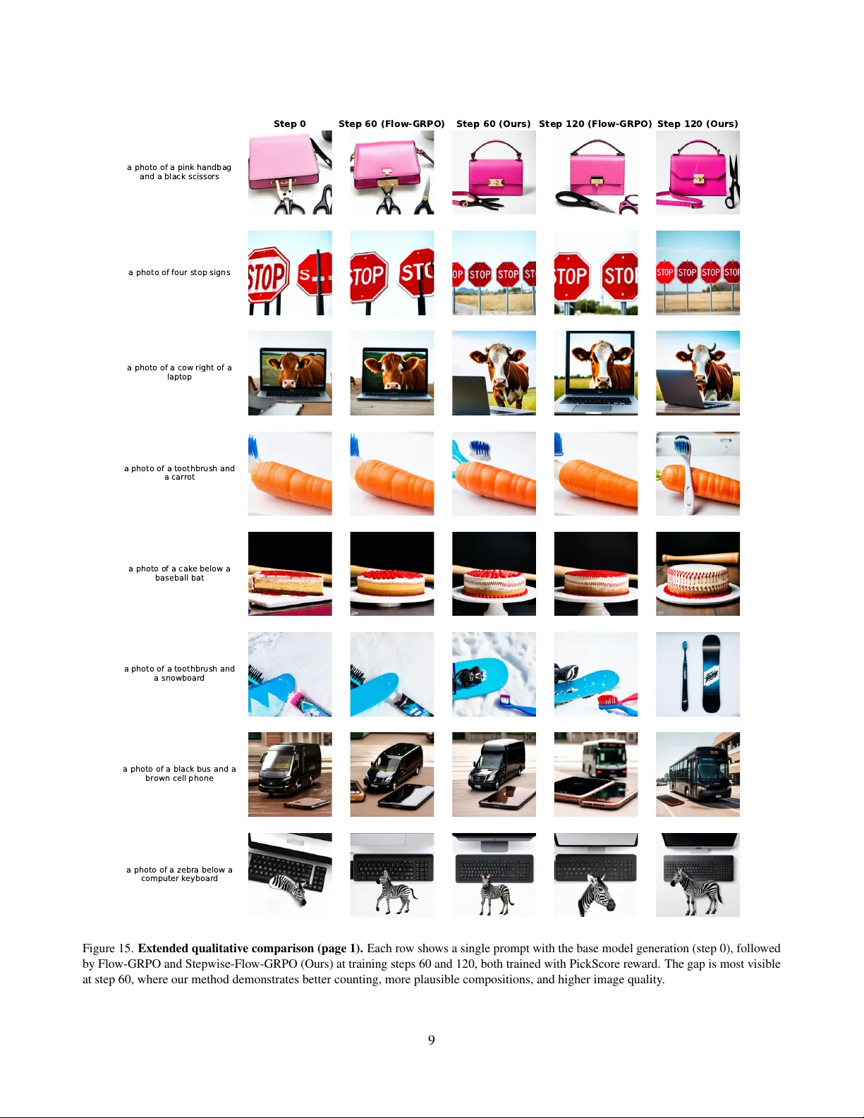
Stepwise Credit Assignment for GRPO on Flow-Matching Models

Stepwise Cr edit Assignment f or GRPO on Flow-Matching Models Y ash Sav ani † * Branislav Kv eton ‡ Y uchen Liu ‡ Y ilin W ang ‡ Jing Shi ‡ Subhojyoti Mukherjee ‡ Nikos Vlassis ‡ Krishna Kumar Singh ‡ † Carnegie Mellon Uni versity ‡ Adobe Research * W ork done while intern at Adobe. Corresponding author: ysavani@cs.cmu.edu . https://stepwiseflowgrpo.com … … 𝑔 0 . 86 0 𝑔 0 . 71 1 ො 𝑥 0 0 ( 𝑡 ) P r o m pt : “ a bl ue be n c h a n d a wh ite c a t” ො 𝑥 0 1 ( 𝑡 ) Figure 1. Stepwise credit assignment from temporal r eward structure. (Left) T wo trajectories for the same prompt, sho wing T weedie estimates ˆ x i 0 ( t ) and their PickScore re wards r i t at each denoising step. The reward curves are non-monotonic and frequently cross—trajectory 0 (blue) dips at t =0 . 86 before recov ering, while trajectory 1 (orange) drops sharply at t =0 . 71 —yet both reach similar final rew ards ( ∼ 0 . 90 ). Uniform credit assignment would treat these trajectories nearly identically , reinforcing the poor intermediate steps along with the good ones. Stepwise-Flow-GRPO instead uses gains g i t = r i t − 1 − r i t to penalize steps that hurt re ward and credit steps that improv e it, regardless of final outcome. (Right) This finer credit assignment yields faster con ver gence and higher final reward compared to Flo w-GRPO. Abstract Flow-GRPO successfully applies r einfor cement learning to flow models, b ut uses uniform credit assignment acr oss all steps. This ignor es the temporal structur e of diffusion gener - ation: early steps determine composition and content (low- fr equency structur e), while late steps r esolve details and textur es (high-fr equency details). Mor eover , assigning uni- form cr edit based solely on the final ima ge can inadvertently re ward suboptimal intermediate steps , especially when error s ar e corr ected later in the diffusion trajectory . W e pr opose Stepwise-Flow-GRPO , whic h assigns credit based on eac h step’ s re war d impr ovement. By levera ging T weedie’ s for- mula to obtain intermediate r ewar d estimates and intr oduc- ing gain-based advantages, our method achieves superior sample efficiency and faster con verg ence. W e also intr oduce a DDIM-inspir ed SDE that impr oves r ewar d quality while pr eserving stochasticity for policy gradients. 1. Introduction Reinforcement learning (RL) has dramatically improved reasoning in large language models (LLMs) [ 41 ], but adapt- ing it to flow-matching models for text-to-image genera- tion remains challenging. Flow-GRPO [ 26 ] and Dance- GRPO [ 56 ] showed that policy gradients can be applied to flow-matching models like SD-3.5-M by conv erting the deterministic flo w ordinary dif ferential equation (ODE) into a stochastic dif ferential equation (SDE) with matched marginals. These approaches assign the same advantage— calculated from the re wards on the final images—to all steps in a trajectory , effecti vely rewarding or penalizing ev ery denoising step based solely on the final generated ima ge. This uniform credit assignment ignores the temporal structur e of all diffusion generation processes, where dif- ferent steps contribute to distinct image properties. Early denoising steps contain primarily low-frequenc y informa- tion, which determines composition and layout, while late steps resolve high-frequenc y details and te xtures. Rew arding 1 an entire trajectory based on final image quality conflates these phases, potentially reinforcing poor early decisions that are compensated for later . As shown in Fig. 1 , interme- diate rew ard estimates reveal substantial temporal structure across steps that uniform credit assignment fails to exploit. T o capitalize on this opportunity , we propose Stepwise- Flow-GRPO , a stepwise credit assignment approach that directly rew ards the contribution of each denoising step. Us- ing T weedie’ s formula [ 9 ], we predict ˆ x 0 ( t ) := E [ x 0 | x t ] from intermediate noisy states x t and re ward these estimates as r t := R ( ˆ x 0 ( t ) , prompt ) . W e then use the stepwise re- ward gain g t = r t − 1 − r t —measuring the amount each step improv es the reward—to calculate the adv antages that are used to optimize the policy with GRPO [ 41 ]. This re- wards each step based on its actual contrib ution rather than final image quality alone. This design offers better credit assignment and improves sample efficiency . Fig. 4 shows that Stepwise-Flow-GRPO achie ves better sample efficienc y during training and con verges f aster . W e also notice that while the Flow-GRPO SDE prov ably matches marginals of the flo w ODE, the images generated with the SDE are noisy . T o account for this, we introduce a new SDE, inspired by DDIM [ 43 ], that produces high- quality images while matching the Flow-ODE Fokker -Planck marginal in the T aylor limit. Since reward models are trained on clean images, the noisy samples from Flow-GRPO’ s SDE degrade re ward signal; our formulation mitigates this, pro- viding a complementary way to accelerate Flow-GRPO. W e make the follo wing contributions: • W e introduce Stepwise-Flow-GRPO, which re wards rela- tiv e gain for each diffusion step instead of just re warding final image. • W e further optimize Flow-GRPO using an impro ved SDE inspired by DDIM to produce less noisy samples. • Our results show that Stepwise-Flo w-GRPO achieves sig- nificantly better sample ef ficiency and con vergence rates than standard Flow-GRPO. 2. Related W ork Reinfor cement learning (RL). RL is an area of machine learning where the goal is to learn a policy that maximizes a long-term re ward in an uncertain en vironment [ 46 ]. The be- ginnings of RL can be traced to model-based approaches for acting under uncertainty , such as Markov decision pr ocesses (MDPs) [ 4 , 33 ] and partially-observable MDPs (POMDPs) [ 42 ]. Because of the generality of the framework, man y RL algorithms hav e been proposed, such as temporal-difference learning [ 45 ], Q-learning [ 51 ], policy gradients [ 52 ], and actor-critic methods [ 47 ]. The main challenge with applying classic RL algorithms, which rely on v alue functions [ 4 ] and Q functions [ 51 ], to modern generativ e AI models is their scale. Therefore, most modern approaches to RL are based on polic y gradients with KL regularization [ 38 , 48 ]. In pr oxi- mal policy optimization (PPO) [ 40 ], a KL-re gularized policy is optimized with respect to a re ward model. This approach has been successfully applied to reinforcement learning from human feedback [ 30 ]. The main challenge with applying PPO in practice is that it requires a fine-grained critic model, which is yet another challenging learning problem to solv e. Gr oup r elative policy optimization (GRPO) [ 41 ] ov ercomes this problem by estimating and standardizing the rew ards using simulation against an en vironment. Our work replaces the total trajectory reward in GRPO with per-step gains, yielding fine-grained credit assignment analogous to a learned critic in PPO—but without requiring a separate critic model. This design is motiv ated by Kveton et al. [ 23 ] , who showed that KL-re gularized policy gradients ov er stepwise gains can learn near -optimal greedy policies when the reward is monotone and submodular in the state, extending classic guarantees from submodular optimization [ 13 , 29 ]. W e are the first to apply this gain-based transfor- mation to GRPO and flo w models, generalizing beyond the on-policy setting of Kveton et al. [ 23 ] to of f-policy optimiza- tion with group-relativ e advantages. RL for image generation. Recent progress in diffusion models [ 7 , 8 , 32 , 35 , 37 ] has led to substantial improve- ments in text-to-image generation, outperforming earlier GAN [ 14 , 21 , 55 ] and V AE-based [ 34 ] methods in both im- age quality and semantic alignment. Among these, flow- matching techniques [ 10 , 24 ] hav e shown strong perfor- mance but still face challenges in achie ving precise image- text alignment and maintaining aesthetic fidelity [ 5 , 19 , 53 ]. T o address these issues, researchers hav e explored methods such as attention manipulation [ 1 , 3 , 6 ], contrastive learn- ing [ 25 ], and asynchronous dif fusion [ 18 ]. While these ap- proaches offer partial impro vements, they often lack robust- ness and generalization. More recently , RL has emerged as a promising direction for enhancing alignment and image quality [ 20 , 26 , 31 , 56 ], which leverages pre-trained VLM models [ 22 , 28 , 50 , 54 ] to measure various aspects related to image quality and text alignment. Flow-GRPO [ 26 ] is a popular RL method that extends GRPO from the te xt domain [ 15 , 41 ] to image gen- eration using dif fusion models, showing notable gains. How- ev er, it only uses rew ards from the final step of generation, ov erlooking the denoising trajectory across steps. T o ov er- come this, we propose Stepwise-Flo w-GRPO, which intro- duces step-wise rew ards throughout the diffusion process, resulting in more fine-grained guidance and superior perfor- mance in image-text alignment and generation quality . Concurrent w orks. T empFlow-GRPO [ 16 ] and Granular- GRPO [ 58 ] also address the credit assignment limitation in Flow-GRPO. While both works recognize that early de- noising steps ha ve an outsized impact on final quality , they approach the problem differently: T empFlo w-GRPO applies hand-designed noise-le vel weighting to final-image adv an- 2 tages, while Granular-GRPO optimizes only the first half of steps. W e optimize telescoping reward gains that are data- driv en and require no manual scheduling or step selection. W e provide a detailed comparison in Sec. F . 3. Background Flow-matching models learn continuous-time normalizing flo ws by training on interpolated data. Gi ven data x 0 ∼ p data and noise x 1 ∼ N (0 , I ) , rectified flow [ 27 ] defines x t = (1 − t ) x 0 + tx 1 for t ∈ [0 , 1] . The model v θ ( x t , t, c ) is trained to predict the velocity field ˙ x t = x 1 − x 0 via L ( θ ) = E t,x 0 ,x 1 [ || ˙ x t − v θ ( x t , t, c ) || 2 ] where c is the prompt for generating x 0 . Generation follows the ODE: dx t = v θ ( x t , t, c ) dt . Starting from noise x 1 ∼ N (0 , I ) at t = 1 and integrating backw ard in time to t = 0 produces samples from the learned distribution. Flow-GRPO enables RL fine-tuning of flow models by con- verting the deterministic ODE into a stochastic SDE. The key insight from Liu et al. [ 27 ] is the construction of an SDE with matched marginals to the ODE based on the F okker-Planck equation. The SDE is given by dx t =  v t ( x t ) ± σ 2 t 2 t ˆ x 1  dt + σ t dw t (1) where ˆ x 1 = x t + (1 − t ) v t ( x t ) is the predicted noise, σ t is an arbitrary noise schedule, v t ( x t ) := v θ ( x t , t, c ) , and dw t is Brownian motion. In the ± operator , + corresponds to the forward process (corruption with noise) and − to the rev erse process (denoising), obtained via Anderson’ s time re versal formula [ 2 ]. This SDE provides stochasticity for RL exploration while preserving the marginals of the original flow . They solve it using the Euler-Maruyama discretization x t − ∆ t := x t −  v t ( x t ) − σ 2 t 2 t ˆ x 1  ∆ t + σ t √ ∆ tϵ (2) where ϵ ∼ N (0 , I ) injects the stochasticity . Therefore, for any step t , the marginal probability for the previous step t − ∆ t is given by π θ ( x t − ∆ t | x t ) = N  x t − ∆ t ; x t −  v t ( x t ) − σ 2 t 2 t ˆ x 1  ∆ t, σ 2 t ∆ tI  (3) In the rest of the paper , we use t ∈ { T , T − 1 , . . . , 1 , 0 } to index discrete steps in the RL objectiv e, whereas the earlier t ∈ [0 , 1] denotes continuous time in the SDE. This notational con venience simplifies our exposition and should be clear from context. The two are related by t cont. = t disc. T and ∆ t disc. = 1 T . Liu et al. [ 26 ] use GRPO [ 41 ] to optimize the policy π θ using group-relative advantages. For each prompt c , they generate N trajectories ( x i T , . . . , x i 0 ) i ∈ [ N ] and rew ard them on the final image in each trajectory only , r i = R ( x i 0 , c ) . W e denote by R ( x, c ) the rew ard of image x giv en prompt c , and experiment with sev eral different reward functions in Sec. 6 . The advantage of trajectory i is A i = r i − mean std where mean = 1 N N X j =1 r j , std = v u u t 1 N N X j =1 ( r j − mean) 2 The policy is updated to locally maximize J ( θ ) = 1 N T N X i =1 T − 1 X t =0 ℓ ( ρ i t ( θ ) , A i ) − β D i,t KL ( π θ || π ref ) (4) where ℓ ( ρ i t ( θ ) , A i ) = min( ρ i t ( θ ) A i , clip( ρ i t ( θ ) , 1 − ϵ, 1 + ϵ ) A i ) is the advantage of trajectory i weighted by the minimum of the unclipped and clipped propensity ratios at step t ρ i t ( θ ) = π θ ( x i t | x i t +1 ,c ) π old ( x i t | x i t +1 ,c ) between the current polic y π θ in Eq. ( 3 ) and sampling policy π old , clip( x, 1 − ϵ, 1 + ϵ ) = max(1 − ϵ, min(1 + ϵ, x )) is a clipping function parameterized by ϵ ∈ [0 , 1] , and D i,t KL ( π θ || π ref ) = D KL ( π θ ( x i t | x i t +1 , c ) || π ref ( x i t | x i t +1 , c )) is the KL penalty between the current policy π θ and initial policy π ref , at step t of trajectory i . GRPO combines two mechanisms to stabilize policy gra- dient optimization: propensity ratio clipping and KL regu- larization. The clipping clip( ρ i t ( θ ) , 1 − ϵ, 1 + ϵ ) bounds the propensity ratio to prevent destructiv ely lar ge policy updates. The KL penalty β D i,t KL ( π θ || π ref ) anchors the learned policy at the initial policy π ref , preserving its general capabilities while adapting to the reward function. T ogether , these cre- ate a trust region that limits how f ar the policy can de viate from both the sampling policy (clipping with π old ) and its initialization (KL with π ref ) [ 38 ]. In the on-policy setting, when π old = π θ at all iterations, the importance ratio becomes ρ i t ( θ ) = 1 , reducing GRPO to KL-regularized polic y gradient regardless of ϵ [ 48 ]. This simplified v ariant is commonly used when trajectories can be generated ef ficiently , as it remov es both the clipping hy- perparameter ϵ and the complexity of importance weighting, while retaining gradient stabilization through the KL term. 3 4. Problems with Unif orm Credit Assignment Flo w-GRPO uses the same advantage A i —calculated on the final image x i 0 —for e very denoising step, treating all steps as equally responsible for final quality . This uniform credit assignment suffers from two fundamental issues that stem from ignoring the temporal structure of diffusion generation. Problem 1: Ignoring hierarchical frequency structure. The diffusion process has inherent temporal hierarchicy: early steps establish composition and layout (low-frequenc y structure), while later steps refine details and textures (high- frequency structure). This hierarchy arises because different spatial frequencies become distinguishable from noise at different times during denoising. T o see why , consider the rectified flow interpolation in frequency space: ˜ x t ( k ) = (1 − t ) ˜ x 0 ( k ) + t ˜ x 1 ( k ) for spatial frequency k . Natural images concentrate energy at lo w frequencies with power spectrum ∝ | k | − α for α > 0 [ 11 , 36 ], while Gaussian noise ˜ x 1 ∼ N (0 , I ) has flat power across all frequencies. The signal-to- noise ratio at frequency k and time t is therefore SNR t ( k ) =  1 − t t  2 1 | k | α . The 1 / | k | α factor means lo w frequencies al ways ha ve higher SNR than high frequencies. As denoising proceeds ( t → 0) , the global prefactor ((1 − t ) /t ) 2 grows, progressiv ely lifting higher frequencies above the noise floor . The result is a coarse-to-fine generation order: at t ≈ 1 , only low-frequenc y information is recoverable; fine details emerge only near t = 0 . Uniform credit assignment ignores this structure, treating a step that determines object layout identically to one that sharpens an edge. Problem 2: Rewarding mistakes that get corrected. A trajectory might make a mistake at t ≈ 1 (like incorrect object color) that later steps correct. If the final image has a high re ward, Flo w-GRPO reinforces all steps—including the early mistakes—potentially exacerbating artifacts and compositional errors that are corrected later . Fig. 1 sho ws this on a real-world example: rew ard trajectories are non- monotonic, with intermediate dips that later recover , yet uniform credit assignment treats all steps equally . 5. Stepwise-Flow-GRPO T o address these problems, we introduce stepwise credit as- signment through two key ideas: (1) estimating intermediate rew ards by predicting clean images from noisy states, and (2) computing adv antages based on per -step rew ard improve- ments rather than the final re ward alone. W e also introduce a nov el SDE that produces higher-quality denoised images. W e now describe each component. 0.0 0.2 0.4 0.6 0.8 1.0 R everse-pr ocess step t 0.00 0.01 0.02 0.03 0.04 0.05 | g t | Mean Mean ± 1 std Figure 2. Gain magnitudes across steps. Mean absolute gain E i [ | g i t | ] measured on 256 GenEval prompts using PickScore. Early steps show larger gains, indicating that compositional decisions driv e most reward impro vement. 5.1. Stepwise Rewards W e cannot directly ev aluate reward models on noisy inter- mediate states x t , but we can estimate the underlying clean image and re ward that prediction. The T weedie formula [ 9 ] provides ˆ x 0 ( t ) := E [ x 0 | x t ] = x t − t ˆ x 1 , where ˆ x 1 is the pre- dicted noise already computed at each step in the generation process in Eq. ( 2 ). This makes the one-step T weedie estimate essentially free. T o get higher-quality estimates, we denoise from x t tow ard x 0 ov er multiple steps. W e discretize the interval [ t, 0] into T ′ steps and solve the flow ODE using forward Euler: starting from x t , we iterativ ely apply the flo w for steps t, t ( T ′ − 1) /T ′ , . . . , t/T ′ , 0 . When T ′ = 1 , this reduces to the one-step T weedie estimate. In practice, we find that T ′ = 5 ODE substeps provide strong re ward signal with minimal additional cost. W e compute stepwise rewards r i t = R ( ˆ x i 0 ( t ) , c ) at each step t of trajectory i , allowing us to ev aluate how interme- diate states progress tow ard high-quality images rather than relying solely on final outcomes. Crucially , each r i t is esti- mated using a single deterministic denoising trajectory of T ′ substeps starting from x i t —no av eraging over multiple samples is needed. Since the denoising from each state x i t is independent, all T rew ard estimates for a trajectory can be computed in parallel (see Sec. D ). 5.2. Stepwise Policy Optimization W e do not optimize stepwise rewards directly , as this would optimize high-scoring intermediary T weedie estimates in- stead of a high-scoring final image. Instead, we compute stepwise gains g i t := r i t − 1 − r i t , which measure each step’ s 4 marginal reward improvement. Steps that increase the re- ward recei ve positive reinforcement while steps that decrease it are penalized. Crucially , these gains telescope P T t =1 g i t = r i 0 − r i T , meaning that maximizing stepwise gains is equiv alent to maximizing the improv ement from initial noise x T to final image x 0 for a fixed initial condition. This connects local per-step optimization to the global objecti ve of maximizing final rew ard. As shown in Fig. 2 , the magnitudes of the gains are initially large and diminish as t → 0 , suggesting that early compositional decisions dri ve most of the re ward improv ement. Under certain submodularity assumptions, greedy maximization of such gains would be pro vably near- optimal (Sec. 5.3 ). Joint normalization preserv es temporal structure. Fol- lowing GRPO, we transform gains into group-relative ad- v antages. A key design choice is whether to normalize gains separately at each step or jointly across all steps. W e choose joint normalization to preserv e the larger magnitudes of early gains, since per -step normalization would artificially inflate noise in later steps where rew ard improvements are small. The group-relativ e advantage at step t of trajectory i is ˜ A i t = g i t − mean std (5) where mean = 1 N T X j,k g j k , std = s 1 N T X j,k ( g j k − mean) 2 for j ∈ { 1 , . . . , N } and k ∈ { 0 , . . . , T − 1 } . W e update the policy to maximize J ( θ ) = 1 N T N X i =1 T − 1 X t =0 h ℓ ( ρ i t ( θ ) , ˜ A i t ) − β D i,t KL ( π θ || π ref ) i (6) where all the terms are defined as in Eq. ( 4 ). The main dif- ference from Flow-GRPO is that uniform adv antages A i are replaced with stepwise adv antages ˜ A i t . The pseudo-code of our method is in Algorithm 1 . All N trajectories within a group share the same initial noise x T , so that re ward dif fer- ences arise solely from the stochastic denoising process. 5.3. Connection to Submodular Optimization Our greedy gain maximization has theoretical grounding in recent adaptiv e submodular optimization results. Consider a simplified on-policy v ariant of our method where π old = π θ (so ρ i t ( θ ) = 1 ) and advantages are replaced by ra w gains g i t . Then the objectiv e reduces to J ( θ ) = 1 N T N X i =1 T X t =1 g i t − β D KL ( π θ || π ref ) (7) Algorithm 1 Stepwise-Flow-GRPO Require: Base policy π ref , prompts P , number of steps T , batch size N , number of substeps T ′ Ensure: Initialize RL polic y π θ ← π ref while not con verged do Sample prompt c ∼ P Initialize x T ∼ N (0 , I ) for i = 1 , . . . , N do x i T ← x T ▷ All trajectories shar e initial noise Generate trajectories ( x i T − 1 , . . . , x i 0 ) ∼ π θ ( ·| c ) autoregressi vely using Eq. ( 2 ) Compute ˆ x i 0 ( t ) using T ′ substeps for all t Compute rew ards r i t ← R t ( ˆ x i 0 ( t ) , c ) for all t Compute gains g i t ← r i t − 1 − r i t for all t Compute ˜ A i t in Eq. ( 5 ) for all t and i Update θ by policy gradient using an AdamW step on loss − J ( θ ) in Eq. ( 6 ) retur n π θ This formula is algebraically equi valent to the adapti ve pol- icy gradient objective in Kveton et al. [ 23 ] . Kv eton et al. [ 23 ] showed that greedy KL-regularized policy gradients can learn near -optimal policies when re ward gains are mono- tone and submodular—analogous to classic guarantees for greedy submodular maximization [ 13 , 29 ]. The key difference from the classic policy gradient is that rather than optimizing the total trajectory re ward (as in Flo w-GRPO), we optimize per -step gains. Our setting gener - alizes Kveton et al. [ 23 ] by allowing of f-policy optimization ( π old  = π θ ) and group-relative advantages, and represents the first application of adaptive gain maximization to GRPO and flow models. While we do not formally verify submodu- larity of our re ward functions, our empirical successes and diminishing gains in Fig. 2 suggest that a submodularity-like structure is present. 5.4. Design V ariations In Sec. A , we explore se veral design alternativ es: (1) cen- tering gains with an exponential moving a verage baseline to reduce temporal variance, (2) generalized adv antage estima- tion (GAE) to let each step receiv e partial credit for future gains it enables, trading of f bias and v ariance via exponential discounting, (3) an ODE-based formulation using progres- siv e distillation between successive T weedie estimates ˆ x 0 ( t ) and ˆ x 0 ( t − 2∆ t ) . While these offer dif ferent computational tradeoffs, the g ain we presented in Sec. 5.2 performs best in our experiments. 5.5. Impro ved Sampling via DDIM-Style Updates The SDE in Eq. ( 1 ) enables RL by injecting the stochasticity needed for exploration, while matching the marginals to the ODE ensures that optimizing the SDE policy also impro ves 5 the deterministic ODE used at inference. Howe ver , we find empirically that the noise injected by the SDE produces visually degraded samples compared to deterministic ODE integration. Since reward models are trained on clean images, this degrades the re ward estimates and slows do wn optimization. W e adopt a DDIM-style sam- pling strategy [ 43 ] that produces higher-quality samples for the re ward model while preserving the stochasticity required for policy gradients. The DDIM update rule interpolates between deterministic and stochastic sampling x t − ∆ t = √ α t − ∆ t ˆ x 0 ( t ) + q β t − ∆ t − σ 2 t ˆ x 1 + σ t ϵ where √ α t − ∆ t is the signal strength, p β t − ∆ t is the noise strength, and σ t controls stochasticity , T o match the marginals of rectified flow x t = (1 − t ) x 0 + tx 1 , we set α t = (1 − t ) 2 and β t = t 2 , yielding x t − ∆ t = (1 − ( t − ∆ t )) ˆ x 0 ( t ) + q ( t − ∆ t ) 2 − σ 2 t ˆ x 1 + σ t ϵ (8) When σ t = 0 , this recov ers the deterministic flow ODE. Exact marginal matching would require the coefficient of ˆ x 1 to be ( t − ∆ t ) − σ 2 t (2 t ) (deriv ed in Sec. B ). The DDIM form p ( t − ∆ t ) 2 − σ 2 t = ( t − ∆ t ) − σ 2 t 2( t − ∆ t ) + O ( σ 4 t ) is a close approximation for small σ t and ∆ t , and produces higher-quality images in practice. W e use σ t = η ( t − ∆ t ) √ 1 − t , where η controls explo- ration strength. This schedule inj ects maximum stochasticity at t = 1 (heavy noise), smoothly anneals to σ t → 0 as t → 0 to recov er the deterministic ODE, and maintains small σ t throughout to match the mar ginal. The result is a Gaussian policy π θ ( x t − 1 | x t , c ) = N ( x t − 1 ; µ t , σ 2 t I ) with mean µ t = (1 − ( t − ∆ t )) ˆ x 0 ( t ) + q ( t − ∆ t ) 2 − σ 2 t ˆ x 1 (9) This allows computing importance ratios ρ i t ( θ ) and KL penal- ties in Eq. ( 4 ). This approach significantly improves visual quality while preserving the ability to optimize via GRPO. A similar result was deri ved in a recent concurrent work [ 49 ]. 6. Experiments Datasets and metrics. Our main experiments are conducted on two datasets: PickScore [ 22 ] and GenEval [ 12 ], which tests compositional understanding through spatial relation- ships, object counts, and attribute binding. W e addition- ally ev aluate OCR text rendering in Sec. E . For the final model validation, we e valuate PickScore-trained models us- ing GenEv al and provide qualitati ve examples of their out- puts to v erify that the y match Flo w-GRPO without rew ard hacking or artifacts. P r o m p t s F l o w - GR P O O u r s A p h o t o o f a d o n u t b e l o w a c a t A p h o t o o f a b u s a b o v e a b o a t A p h o t o o f a c o w ri g h t o f a l a p t o p A p h o t o o f a b ro w n h o t d o g a n d a p u rp l e p i z z a A p h o t o o f a p i n k o v e n a n d a g re e n m o t o r c y c l e A p h o t o o f f o u r f ri s b e s s Figure 3. Qualitati ve results . W e compare our Stepwise-Flow- GRPO with Flo w-GRPO and observe better spatial reasoning, at- tribute binding, and counting performance. Reward functions. On GenEval, we train with three pre- trained re ward models: PickScore [ 22 ], ImageRe ward [ 54 ], and UnifiedRew ard-7b-v1.5 [ 50 ]. On the PickScore dataset, we use PickScore as the rew ard. UnifiedReward requires 8 additional NVIDIA A100 80GB GPUs, deployed via SGLang [ 57 ] for ef ficient inference (prompt in Sec. E ). All rew ard functions use the default Flow-GRPO implementa- tion with efficienc y optimizations. Implementation details. W e use SD3.5-Medium [ 44 ] trained on 8 NVIDIA A100 GPUs, built from the Flow- GRPO codebase [ 26 ]. W e sample using 10 denoising steps with cfg = 1 . 0 [ 17 ] (no classifier-free guidance) and batch size 16 to maximize throughput and double training batch 6 0 50 100 150 Step 0.725 0.750 0.775 0.800 0.825 0.850 0.875 0.900 PickScore Ours Flow-GRPO (a) Pickscore (GenEval) 0 50 100 150 Step 0.2 0.4 0.6 0.8 ImageReward Ours Flow-GRPO (b) ImageRew ard (GenEval) 0 50 100 150 200 Step 0.2 0.3 0.4 0.5 0.6 UnifiedReward Ours Flow-GRPO (c) UnifiedRew ard (GenEval) 0 50 100 150 Step 0.700 0.725 0.750 0.775 0.800 0.825 0.850 PickScore Ours Flow-GRPO (d) PickScore (PickScore Dataset) Figure 4. Sample efficiency across r eward functions. Stepwise-Flow-GRPO consistently outperforms Flow-GRPO in re ward per training step across all settings, achieving both f aster conv ergence and superior final performance in 3 out of 4 settings. 0 50 100 150 0.725 0.750 0.775 0.800 0.825 0.850 0.875 0.900 PickScore Ours Flow-GRPO Wall-clock time (min) (a) Pickscore (GenEval) 0 25 50 75 100 0.2 0.4 0.6 0.8 ImageReward Ours Flow-GRPO Wall-clock time (min) (b) ImageRew ard (GenEval) 0 50 100 150 200 Wall-clock time (min) 0.2 0.3 0.4 0.5 0.6 UnifiedReward Ours Flow-GRPO (c) UnifiedRew ard (GenEval) 0 25 50 75 100 Wall-clock time (min) 0.675 0.700 0.725 0.750 0.775 0.800 0.825 0.850 0.875 PickScore Ours Flow-GRPO (d) Pickscore (PickScore Dataset) Figure 5. W all-clock efficiency matches sample efficiency gains. Reward v ersus wall-clock time for the same settings as Fig. 4 . Despite additional computational cost for intermediate denoising, Stepwise-Flow-GRPO conv erges faster in wall-clock time, achieving visibly superior performance in 3 out of 4 settings. 0 50 100 Step 0.75 0.80 0.85 0.90 PickScore Ours Flow-GRPO Ours (Imp. SDE) Flow-GRPO (Imp. SDE) (a) PickScore (GenEval) 0 50 100 150 Step 0.2 0.4 0.6 0.8 ImageReward Ours Flow-GRPO Ours (Imp. SDE) Flow-GRPO (Imp. SDE) (b) ImageRew ard (GenEval) 0 50 100 150 200 Step 0.2 0.3 0.4 0.5 0.6 0.7 UnifiedReward Ours Flow-GRPO Ours (Imp. SDE) Flow-GRPO (Imp. SDE) (c) UnifiedRew ard (GenEval) 0 50 100 150 200 Step 0.70 0.75 0.80 0.85 0.90 PickScore Ours Flow-GRPO Ours (Imp. SDE) Flow-GRPO (Imp. SDE) (d) Pickscore (PickScore Dataset) Figure 6. Stepwise credit assignment r emains effective with impro ved SDE. Reward versus training step when both methods use the DDIM-inspired SDE from Sec. 5.5 . Stepwise-Flo w-GRPO retains its sample efficienc y advantage, demonstrating that the improvements in credit assignment and sampling are complementary . sizes. For the SDE formulation, we use σ t = 0 . 7 p t/ (1 − t ) following Flo w-GRPO, and additionally ev aluate both meth- ods with our improved SDE from Sec. 5.5 using η = 0 . 9 . Our method computes intermediate estimates ˆ x 0 ( t ) using T ′ = 5 flow ODE substeps from each x t . T o assess final model quality under standard inference settings, we sep- arately train models with cfg = 4 . 5 and batch size 8 us- ing PickScore on the GenEval dataset, and ev aluate with the GenEval benchmark (reward and wall-clock figures in Sec. E ). 6.1. Main Results Sample efficiency . Fig. 4 shows that Stepwise-Flow-GRPO consistently achieves higher rew ards for the final image 7 Experiment Overall Single Obj. T wo Objs. Counting Colors Position Attr . Binding Pr etrained Models SD3.5-M (cfg=1.0) 0.28 0.71 0.23 0.15 0.45 0.05 0.08 SD3.5-M (cfg=4.5) 0.63 0.98 0.78 0.50 0.81 0.24 0.52 F ine-tuned Models SD3.5-M+Flow-GRPO (cfg=1.0 PickScore) 0.60 0.96 0.73 0.67 0.67 0.21 0.35 SD3.5-M+Ours (cfg=1.0 PickScore) 0.60 0.96 0.75 0.67 0.67 0.21 0.34 SD3.5-M+Flow-GRPO (cfg=4.5 Pickscore) 0.68 0.98 0.82 0.64 0.82 0.24 0.59 SD3.5-M+Ours (cfg=4.5 PickScore) 0.71 0.98 0.85 0.70 0.82 0.29 0.59 T able 1. Final model quality on GenEval. Compositional generation performance for models trained with PickScore re ward. Both methods substantially improve o ver the base model, with our method matching Flow-GRPO at cfg=1.0 and outperforming it across most categories at cfg=4.5, particularly in counting and spatial positioning. per training iteration than Flow-GRPO across all reward functions, demonstrating superior sample efficiency . The improv ement is most pronounced early in training, where stepwise credit assignment enables faster identification of effecti ve denoising strategies. Our method achiev es both faster con ver gence and superior final performance in 3 out of 4 settings. Importantly , T ab . 1 sho ws that despite faster con vergence, our method achiev es no worse final GenEval accuracy than Flo w-GRPO, indicating we improve learning speed without sacrificing final quality . W all-clock efficiency . While Stepwise-Flow-GRPO requires additional computation for intermediate denoising and re- ward e valuation (timing breakdo wn in Sec. D ), the impro ved sample efficiency compensates for this overhead. Fig. 5 shows that our method con verges f aster in wall-clock time, achie ving visibly superior performance in 3 out of 4 settings, reaching target reward values with less total computation than Flow-GRPO. GenEval results. Our Stepwise-Flow-GRPO matches Flow- GRPO at cfg=1.0 and outperforms it at cfg=4.5 (it is equal or better on all sub-categories) in T ab . 1 . W e compare the methods qualitativ ely in Fig. 3 . The results indicate that our method improv es spatial reasoning, attribute binding, and counting capabilities. The generated images also appear to be more realistic and physically plausible. Notably , Flow- GRPO merges objects in the first and fifth ro ws, and places the bus unrealistically in the sky instead of on the top of the boat in the third row . Additional qualitativ e examples are giv en in Sec. E . Impro ved SDE results. Fig. 6 shows that Stepwise-Flow- GRPO has better sample efficienc y than Flow-GRPO when both methods use the impro ved SDE from Sec. 5.5 . While the DDIM-inspired SDE substantially impro ves both meth- ods, combining it with stepwise credit assignment yields better results than either modification alone, showing that the improv ements are complementary . 6.2. Ablation Studies Number of denoising substeps. W e ablate the number of ODE steps T ′ used to estimate ˆ x 0 ( t ) in Sec. C . When 1 ≤ T ′ ≤ 3 , the reward estimates are noisy and degrade training signal, while 6 ≤ T ′ ≤ 10 hav e negligible quality improv ements at increased computational cost. W e select T ′ = 5 as the optimal tradeoff between estimate quality and efficienc y . Gain normalization strategy . W e compare joint normal- ization in Eq. ( 5 ) to per -step normalization in Sec. C . Joint normalization preserves the temporal structure where early gains are lar ger (Fig. 2 ), allo wing optimization to prioritize compositional decisions over detail refinement. Per-step nor - malization equalizes importance across the steps, resulting in slower con vergence (see Sec. C ). 7. Conclusions and Future W ork W e introduced Stepwise-Flow-GRPO, which assigns credit to individual denoising steps using gain-based advantages from intermediate re ward estimates, and a DDIM-inspired SDE that improves re ward signal quality . T ogether , these yield superior sample efficienc y , con vergence speed, and training stability ov er uniform credit assignment. Our stepwise gains open sev eral directions: using per- prompt gain variance as a difficulty signal for curriculum learning, adaptively weighting steps proportional to their gain v ariance to focus optimization on high-information re- gions of the trajectory , and enabling self-correcting diffusion where models learn to detect and retry poor intermediate decisions. 8 References [1] Aishwarya Agarwal, Srikrishna Karanam, K. J. Joseph, Apoorv Saxena, K oustav a Goswami, and Balaji V asan Srini- vasan. A-star: T est-time attention segre gation and retention for text-to-image synthesis. 2023 IEEE/CVF International Confer ence on Computer V ision (ICCV) , pages 2283–2293, 2023. 2 [2] B. D. O. Anderson. Rev erse-time diffusion equation models. Stochastic Pr ocesses and their Applications , 12(3):313–326, 1982. 3 [3] Zhipeng Bao, Y ijun Li, Krishna Kumar Singh, Y u-Xiong W ang, and Martial Hebert. Separate-and-enhance: Com- positional finetuning for text2image diffusion models. In SIGGRAPH , 2024. 2 [4] Richard Bellman. Dynamic Pro gramming . Princeton Univ er- sity Press, Princeton, NJ, 1957. 2 [5] Agneet Chatterjee, Gabriela Ben Melech Stan, Estelle Aflalo, Sayak Paul, Dhruba Ghosh, T ejas Gokhale, Ludwig Schmidt, Hannaneh Hajishirzi, V asudev Lal, Chitta Baral, and Y ezhou Y ang. Getting it right: Improving spatial consistency in te xt- to-image models, 2024. 2 [6] Hila Chefer , Y uval Alaluf, Y ael V inker , Lior W olf, and Daniel Cohen-Or . Attend-and-excite: Attention-based semantic guid- ance for text-to-image dif fusion models, 2023. 2 [7] Junsong Chen, Jincheng Y u, Chongjian Ge, Lewei Y ao, Enze Xie, Y ue W u, Zhongdao W ang, James Kwok, Ping Luo, Huchuan Lu, and Zhenguo Li. Pixart- α : Fast training of diffusion transformer for photorealistic te xt-to-image synthe- sis, 2023. 2 [8] Prafulla Dhariwal and Ale xander Nichol. Diffusion models beat gans on image synthesis. Advances in neural information pr ocessing systems , 2021. 2 [9] Bradley Efron. T weedie’ s formula and selection bias. Journal of the American Statistical Association , 106(496):1602–1614, 2011. 2 , 4 [10] Patrick Esser , Sumith Kulal, Andreas Blattmann, Rahim En- tezari, Jonas Müller , Harry Saini, Y am Levi, Dominik Lorenz, Axel Sauer , Frederic Boesel, Dustin Podell, T im Dockhorn, Zion English, Kyle Lacey , Ale x Goodwin, Y annik Marek, and Robin Rombach. Scaling rectified flow transformers for high- resolution image synthesis. arXiv preprint , 2024. 2 [11] David J. Field. Relations between the statistics of natural images and the response properties of cortical cells. Journal of the Optical Society of America A , 4(12):2379–2394, 1987. 4 [12] Dhruba Ghosh, Hannaneh Hajishirzi, and Ludwig Schmidt. Genev al: An object-focused framew ork for ev aluating text-to- image alignment. Advances in Neural Information Pr ocessing Systems , 36:52132–52152, 2023. 6 [13] Daniel Golovin and Andreas Krause. Adaptive submodularity: Theory and applications in activ e learning and stochastic optimization. Journal of Artificial Intellig ence Resear ch , 42: 427–486, 2011. 2 , 5 [14] Ian J Goodfellow , Jean Pouget-Abadie, Mehdi Mirza, Bing Xu, David W arde-Farley , Sherjil Ozair , Aaron Courville, and Y oshua Bengio. Generati ve adversarial nets. Advances in neural information pr ocessing systems , 27, 2014. 2 [15] Daya Guo, Dejian Y ang, Hao wei Zhang, Junxiao Song, Ruoyu Zhang, Runxin Xu, Qihao Zhu, Shirong Ma, Peiyi W ang, Xiao Bi, et al. Deepseek-r1: Incentivizing reasoning capability in llms via reinforcement learning. arXiv pr eprint arXiv:2501.12948 , 2025. 2 [16] Xiaoxuan He, Siming Fu, Y uke Zhao, W anli Li, Jian Y ang, Dacheng Y in, Fengyun Rao, and Bo Zhang. T empflo w-grpo: When timing matters for grpo in flow models. arXiv preprint arXiv:2508.04324 , 2025. 2 , 6 [17] Jonathan Ho and Tim Salimans. Classifier-free diffusion guidance. arXiv pr eprint arXiv:2207.12598 , 2022. 6 [18] Zijing Hu, Y unze T ong, Fengda Zhang, Junkun Y uan, Jun Xiao, and Kun Kuang. Asynchronous denoising diffusion models for aligning text-to-image generation, 2025. 2 [19] Kaiyi Huang, Kaiyue Sun, Enze Xie, Zhenguo Li, and Xihui Liu. T2i-compbench: A comprehensiv e benchmark for open- world compositional te xt-to-image generation. Advances in Neural Information Pr ocessing Systems , 2023. 2 [20] Dongzhi Jiang, Ziyu Guo, Renrui Zhang, Zhuofan Zong, Hao Li, Le Zhuo, Shilin Y an, Pheng-Ann Heng, and Hong- sheng Li. T2i-r1: Reinforcing image generation with col- laborativ e semantic-level and token-le vel cot. arXiv pr eprint arXiv:2505.00703 , 2025. 2 [21] Minguk Kang, Jun-Y an Zhu, Richard Zhang, Jaesik Park, Eli Shechtman, Sylv ain Paris, and T aesung Park. Scaling up gans for text-to-image synthesis. In Pr oceedings of the IEEE Con- fer ence on Computer V ision and P attern Recognition (CVPR) , 2023. 2 [22] Y uval Kirstain, Adam Polyak, Uriel Singer , Shahbuland Ma- tiana, Joe Penna, and Omer Levy . Pick-a-pic: An open dataset of user preferences for text-to-image generation. 2023. 2 , 6 [23] Branislav Kveton, Anup Rao, V iet Dac Lai, Nikos Vlassis, and David Arbour . Adaptiv e submodular policy optimization. In Proceedings of the 2nd Reinforcement Learning Confer- ence , 2025. 2 , 5 [24] Black F orest Labs, Stephen Batifol, Andreas Blattmann, Fred- eric Boesel, Saksham Consul, Cyril Diagne, T im Dockhorn, Jack English, Zion English, Patrick Esser , Sumith Kulal, Kyle Lacey , Y am Levi, Cheng Li, Dominik Lorenz, Jonas Müller, Dustin Podell, Robin Rombach, Harry Saini, Axel Sauer, and Luke Smith. Flux.1 kontext: Flow matching for in-context image generation and editing in latent space, 2025. 2 [25] Jaa-Y eon Lee, Byunghee Cha, Jeongsol Kim, and Jong Chul Y e. Aligning text to image in dif fusion models is easier than you think, 2025. 2 [26] Jie Liu, Gongye Liu, Jiajun Liang, Y angguang Li, Jiaheng Liu, Xintao W ang, Pengfei W an, Di Zhang, and W anli Ouyang. Flow-grpo: T raining flow matching models via online rl. arXiv pr eprint arXiv:2505.05470 , 2025. 1 , 2 , 3 , 6 , 7 [27] Xingchao Liu, Chengyue Gong, and Qiang Liu. Flow straight and fast: Learning to generate and transfer data with rectified flow . arXiv preprint , 2022. 3 [28] Y uhang Ma, Xiaoshi W u, Keqiang Sun, and Hongsheng Li. Hpsv3: T ow ards wide-spectrum human preference score, 2025. 2 9 [29] G. L. Nemhauser , L. A. W olsey , and M. L. Fisher . An analysis of approximations for maximizing submodular set functions - I. Mathematical Pr ogramming , 14(1):265–294, 1978. 2 , 5 [30] Long Ouyang, Jeffre y W u, Xu Jiang, Diogo Almeida, Carroll W ainwright, Pamela Mishkin, Chong Zhang, Sandhini Agar- wal, Katarina Slama, Ale x Ray , John Schulman, Jacob Hilton, Fraser Kelton, Luk e Miller, Maddie Simens, Amanda Ask ell, Peter W elinder, P aul Christiano, Jan Leike, and Ryan Lo we. T raining language models to follow instructions with human feedback. In Advances in Neural Information Pr ocessing Systems 35 , 2022. 2 [31] Kaihang Pan, W endong Bu, Y uruo Wu, Y ang Wu, Kai Shen, Y unfei Li, Hang Zhao, Juncheng Li, Siliang T ang, and Y ueting Zhuang. Focusdiff: Advancing fine-grained te xt-image align- ment for autoregressiv e visual generation through rl. arXiv pr eprint arXiv:2506.05501 , 2025. 2 [32] Dustin Podell, Zion English, Kyle Lacey , Andreas Blattmann, T im Dockhorn, Jonas Müller , Joe Penna, and Robin Rombach. Sdxl: Improving latent diffusion models for high-resolution image synthesis. In The T welfth International Confer ence on Learning Repr esentations (ICLR) , 2024. 2 [33] Martin Puterman. Markov Decision Processes: Discrete Stochastic Dynamic Pr ogramming . John W iley & Sons, New Y ork, NY , 1994. 2 [34] Aditya Ramesh, Mikhail Pavlo v , Gabriel Goh, Scott Gray , Chelsea V oss, Alec Radford, Mark Chen, and Ilya Sutskev er . Zero-shot text-to-image generation. In Pr oceedings of the 38th International Confer ence on Machine Learning . PMLR, 2021. 2 [35] Robin Rombach, Andreas Blattmann, Dominik Lorenz, Patrick Esser, and Björn Ommer. High-resolution image synthesis with latent diffusion models. In Proceedings of the IEEE/CVF Confer ence on Computer V ision and P attern Recognition (CVPR) , 2022. 2 [36] Daniel L. Ruderman and William Bialek. Statistics of natural images: Scaling in the woods. Physical Review Letters , 73 (6):814–817, 1994. 4 [37] Chitwan Saharia, William Chan, Saurabh Saxena, Lala Li, Jay Whang, Emily L Denton, Kamyar Ghasemipour, Raphael Gontijo Lopes, Burcu Karagol A yan, Tim Salimans, et al. Pho- torealistic text-to-image dif fusion models with deep language understanding. Advances in neural information pr ocessing systems , 2022. 2 [38] John Schulman, Serge y Levine, Pieter Abbeel, Michael Jor- dan, and Philipp Moritz. Trust region policy optimization. In Pr oceedings of the 32nd International Confer ence on Ma- chine Learning , pages 1889–1897, 2015. 2 , 3 [39] John Schulman, Philipp Moritz, Serge y Levine, Michael Jor - dan, and Pieter Abbeel. High-dimensional continuous con- trol using generalized adv antage estimation. arXiv preprint arXiv:1506.02438 , 2015. 1 [40] John Schulman, Filip W olski, Prafulla Dhariwal, Alec Rad- ford, and Oleg Klimov . Proximal policy optimization algo- rithms. CoRR , abs/1707.06347, 2017. 2 [41] Zhihong Shao, Peiyi W ang, Qihao Zhu, Runxin Xu, Junxiao Song, Xiao Bi, Hao wei Zhang, Mingchuan Zhang, Y . K. Li, Y . Wu, and Daya Guo. DeepSeekMath: Pushing the limits of mathematical reasoning in open language models. CoRR , abs/2402.03300, 2024. 1 , 2 , 3 [42] Edward Sondik. The Optimal Contr ol of P artially Observable Markov Decision Pr ocesses . PhD thesis, Stanford University , 1971. 2 [43] Jiaming Song, Chenlin Meng, and Stef ano Ermon. Denoising diffusion implicit models. In International Conference on Learning Repr esentations (ICLR) , 2021. 2 , 6 [44] Stability AI. Stable diffusion 3.5: A multimodal diffusion transformer , 2024. 6 [45] Richard Sutton. Learning to predict by the methods of tempo- ral differences. Machine Learning , 3:9–44, 1988. 2 [46] Richard Sutton and Andrew Barto. Reinforcement Learning: An Intr oduction . MIT Press, Cambridge, MA, 1998. 2 [47] Richard Sutton, David McAllester , Satinder Singh, and Y ishay Mansour . Policy gradient methods for reinforcement learning with function approximation. In Advances in Neural Information Pr ocessing Systems 12 , pages 1057–1063, 2000. 2 [48] Emanuel T odorov . Linearly-solvable Markov decision prob- lems. In Advances in Neural Information Processing Systems 19 , 2006. 2 , 3 [49] Feng W ang and Zihao Y u. Coefficients-preserving sampling for reinforcement learning with flow matching, 2025. 6 [50] Y ibin W ang, Y uhang Zang, Hao Li, Cheng Jin, and Jiaqi W ang. Unified reward model for multimodal understanding and generation. arXiv preprint , 2025. 2 , 6 [51] Christopher W atkins and Peter Dayan. Q-learning. Machine Learning , 8:279–292, 1992. 2 [52] Ronald W illiams. Simple statistical gradient-following al- gorithms for connectionist reinforcement learning. Machine Learning , 8(3-4):229–256, 1992. 2 [53] Xindi W u, Dingli Y u, Y angsibo Huang, Olga Russakovsky , and Sanjeev Arora. Conceptmix: A compositional image generation benchmark with controllable difficulty . arXiv pr eprint arXiv:2408.14339 , 2024. 2 [54] Jiazheng Xu, Xiao Liu, Y uchen Wu, Y uxuan T ong, Qinkai Li, Ming Ding, Jie T ang, and Y uxiao Dong. Imagere ward: learning and ev aluating human preferences for text-to-image generation. In Pr oceedings of the 37th International Con- fer ence on Neural Information Pr ocessing Systems , 2023. 2 , 6 [55] T ao Xu, Pengchuan Zhang, Qiuyuan Huang, Han Zhang, Zhe Gan, Xiaolei Huang, and Xiaodong He. Attngan: Fine- grained text to image generation with attentional generativ e adversarial networks. arXiv pr eprint arXiv:1711.10485 , 2017. 2 [56] Zeyue Xue, Jie W u, Y u Gao, Fangyuan K ong, Lingting Zhu, Mengzhao Chen, Zhiheng Liu, W ei Liu, Qiushan Guo, W eilin Huang, et al. Dancegrpo: Unleashing grpo on visual genera- tion. arXiv pr eprint arXiv:2505.07818 , 2025. 1 , 2 [57] Lianmin Zheng, Liangsheng Y in, Zhiqiang Xie, Jef f Huang, Chuyue Sun, Cody Hao Y u, Shiyi Cao, Christos Kozyrakis, Ion Stoica, Joseph E. Gonzalez, Clark Barrett, and Y ing Sheng. Efficiently programming large language models using sglang, 2023. 6 10 [58] Y ujie Zhou, Pengyang Ling, Jiazi Bu, Y ibin W ang, Y uhang Zang, Jiaqi W ang, Li Niu, and Guangtao Zhai. Fine-grained grpo for precise preference alignment in flow models. arXiv pr eprint arXiv:2510.01982 , 2025. 2 , 6 11 Stepwise Cr edit Assignment f or GRPO on Flow-Matching Models Supplementary Material In this appendix, we cover the following topics: A) our exploration on v arious design choices B) our improv ement on SDE C) ablation studies D) our runtime analysis E) addi- tional results F) comparisons with concurrent work. A. Design V ariations W e explored several alternative formulations of stepwise credit assignment to in vestigate potential improvements in variance reduction and temporal credit propagation. While these v ariations offer intuiti ve benefits in principle, our exper - iments show that the gain formulation from Sec. 5.2 performs best in practice. A.1. Exponential Moving A verage Baseline Motivation. Raw gains g i t = r i t − 1 − r i t can exhibit high variance across training iterations, potentially leading to noisy gradient estimates. A common variance reduction technique in RL is to center advantages using a baseline. W e explore using an e xponential moving a verage (EMA) of past gains as a temporal baseline. Formulation. W e maintain a per -step EMA baseline b t updated after each training iteration: b t ← α · b t + (1 − α ) · E i [ g i t ] (10) where α = 0 . 99 is the decay rate. The centered gains are then: ˜ g i t = g i t − b t (11) These centered gains are normalized and con verted to adv an- tages as in the standard formulation. Expected benefit. By subtracting a running average of typical gain magnitudes at each step, we hoped to reduce vari- ance in advantage estimates while preserving the directional signal about which steps improve re ward. This is analogous to value function baselines in polic y gradient methods. A.2. Generalized Advantage Estimation (GAE) Motivation. Standard gains g i t only capture the immediate rew ard improvement from step t . Howe ver , a step’ s true contribution might include its do wnstream impact on future steps. GAE [ 39 ] provides a principled way to trade of f bias and variance by e xponentially weighting future gains. Formulation. W e apply GAE to the gain sequence with discount factor γ : GAE i t = T − t X k =0 γ k g i t + k (12) In practice, we compute this efficiently via: GAE i t = 1 γ t T X k = t γ k g i k (13) W e use γ = 0 . 95 following standard RL practice. The GAE values replace ra w gains in the advantage calculation. Expected benefit. GAE allows early steps to receiv e credit for setting up conditions that enable large future gains, ev en if their immediate gain g i t is small. F or example, a compositional decision at t ≈ T might have small imme- diate reward improvement but enable larger gains at later refinement steps. W e hypothesized this could improve credit assignment for temporally extended ef fects. A.3. ODE-Based Progr essive Distillation Motivation. The SDE formulation requires introducing stochasticity σ t for policy gradients, which can de grade sam- ple quality . An alternative approach is to av oid the SDE entirely and instead optimize a progressi ve distillation objec- tiv e between successiv e T weedie estimates. Formulation. Instead of computing log-probabilities under a Gaussian policy , we use a progressive distillation loss between the current step’ s T weedie estimate ˆ x 0 ( t ) and the twice-previous step’ s estimate ˆ x 0 ( t − 2∆ t ) : L i t = −∥ ˆ x i 0 ( t − 2∆ t ) − µ i t ∥ 2 (14) where µ i t is the mean of the flow transition from x t to x t − 2∆ t : µ i t = ˆ x i 0 ( t ) · (1 − ( t − 2∆ t )) + ˆ x i 1 ( t ) · ( t − 2∆ t ) (15) W e then scale this loss by gain-based adv antages as in stan- dard GRPO. Expected benefit. This formulation completely avoids the stochasticity required for the SDE, potentially impro ving sample quality . The distillation objective encourages consis- tency between successive predictions of the final image, with stronger enforcement on steps with high gains. W e hypothe- sized this could provide cleaner gradients while maintaining stepwise credit assignment. A.4. Experimental Results W e ev aluate all variations on the PickScore reward using the GenEv al dataset, follo wing the same training protocol as our main experiments. Fig. 7 shows re ward curves for all design v ariations com- pared to our standard gain formulation. No variation sho ws significant improv ement over the standard formulation. 1 0 50 100 150 Step 0.75 0.80 0.85 0.90 PickScore Ours EMA gains GAE gains ODE Figure 7. Design variation comparison. Rew ard vs. training iteration for different formulations of stepwise credit assignment on GenEval with PickScore re ward. The standard gain formulation from the main paper matches all alternatives, demonstrating that preserving the natural temporal structure of dif fusion gains is the most effecti ve credit assignment. The superior performance of using advantage calculated directly on the gains suggests that the natural temporal struc- ture of diffusion generation should be preserv ed rather than normalized aw ay . EMA centering and GAE both don’t sig- nificantly improv e with this structure, while progressive dis- tillation is far less stable than the SDE formulation. So, in the main paper we keep the original, simpler implementation. B. Impro ved SDE Flow-GRPO’ s SDE generates noisy intermediate samples that degrade re ward signal quality . While the SDE in Eq. ( 1 ) is theoretically sound for RL exploration, the noise injection mechanism produces visibly corrupted images at interme- diate steps, see Fig. 8 . Since rew ard models are typically trained on clean images, this noise substantially reduces the informativ eness of reward signals, slo wing RL con ver gence. W e address this by replacing Flow-GRPO’ s SDE with a DDIM-inspired alternati ve that provides e xploration while producing cleaner samples. W e construct an SDE that interpolates between deter- ministic ODE sampling and stochastic exploration while preserving the variance structure of the flo w . Drawing inspi- ration from DDIM [ 43 ], we define the transition from step t to t − ∆ t as x t − ∆ t = (1 − ( t − ∆ t )) ˆ x 0 + q ( t − ∆ t ) 2 − σ 2 t ˆ x 1 + σ t ϵ (16) where ˆ x 0 = x t − tv t and ˆ x 1 = x t + (1 − t ) v t are the predicted clean image and noise respectively gi ven the flow prediction v t := v θ ( x t , t, c ) . Stochasticity is controlled with σ t and ϵ ∼ N (0 , I ) . When σ t = 0 , this recov ers the deterministic ODE; when σ t > 0 , RL exploration is enabled through controlled noise injection. 1 Re writing Eq. ( 2 ) using x t = (1 − t ) ˆ x 0 + t ˆ x 1 , we obtain x t − ∆ t = (1 − ( t − ∆ t )) ˆ x 0 +  ( t − ∆ t ) + σ 2 t ∆ t 2 t  ˆ x 1 + σ t √ ∆ t ϵ (17) Comparing with Eq. ( 16 ), the noise coefficients differ by p ( t − ∆ t ) 2 − σ 2 t ≈ ( t − ∆ t ) − σ 2 t 2( t − ∆ t ) via T aylor ex- pansion. As ∆ t → 0 and σ t → 0 , the two formulations con verge. B.1. V ariance-Preserving Pr operty The DDIM SDE exactly preserv es the marginal variance at each step, while Flow-GRPO’ s SDE inflates it. For rectified flo w , the training interpolation x t = (1 − t ) x 0 + tx 1 implies that V ar( x t | x 0 ) = t 2 . Computing the variance of Eq. ( 16 ): V ar( x t − ∆ t | ˆ x 0 ) (18) = (( t − ∆ t ) 2 − σ 2 t ) V ar( ˆ x 1 ) + σ 2 t (19) If V ar( ˆ x 1 ) = 1 , this exactly matches the e xpected variance. In contrast, from Eq. ( 17 ): V ar Flow ( x t − ∆ t | x 0 ) =  ( t − ∆ t ) + σ 2 t ∆ t 2 t  2 + σ 2 t ∆ t > ( t − ∆ t ) 2 for any σ t > 0 , ∆ t > 0 (20) This excess variance accumulates across steps, producing visibly noisier trajectories that confound rew ard ev aluation. B.2. Adaptive Noise Schedule Setting σ 2 t = ( t − ∆ t ) 2 in Eq. ( 16 ) yields: x t − ∆ t = (1 − ( t − ∆ t )) ˆ x 0 + ( t − ∆ t ) ϵ (21) which completely discards the predicted noise ˆ x 1 . Howe ver , during training, the model learns that x t = (1 − t ) x 0 + tx 1 where both x 0 and x 1 contain complementary information about the data distribution. At test time, both ˆ x 0 and ˆ x 1 carry 1 This is exactly equal to the DDIM update if we let α t − ∆ t = (1 − ( t − ∆ t )) 2 and β t = ( t − ∆ t ) 2 , where α t and β t are the signal and noise strengths in the paper respectiv ely . 2 P r o m p t s F l o w - GR P O S D E I m p r o v e d S D E a p h o t o o f t w o w i n e g l a s s e s a p h o t o o f a b o w l a p h o t o o f a y e l l o w d i n i n g t a b l e a n d a p i n k d o g a p h o t o o f a b r o w n c a rro t a n d a w h i t e p o t t e d p l a n t a p h o t o o f a c o w ri g h t o f a l a p t o p Figure 8. Improved SDE produces cleaner images. Qualitativ e comparison between Flow-GRPO SDE (middle) and our DDIM- inspired SDE (right) from Sec. 5.5 . The improved formulation gen- erates images that are much less noisy while maintaining stochas- ticity for policy gradients. entangled information about the true clean image, i.e., ˆ x 1 is not merely noise to be replaced, but rather encodes structure that the model has learned to extract from x t . Fully replac- ing ˆ x 1 with independent noise ϵ produces samples of the form (1 − t ) ˆ x 0 + tϵ , which lie outside the model’ s training distribution and yield poor v elocity predictions v t . Setting σ t = η ( t − ∆ t ) retains a (1 − η 2 ) fraction of the predicted noise structure. This interpolates between deterministic sampling ( η = 0 ) and full replacement ( η = 1 ), providing RL e xploration while maintaining samples within the model’ s learned distribution. Howe ver , this uniform schedule treats all steps equally despite their differential impact on the final output. Noise injected at step t propagates through the remaining denoising steps and affects x 0 through the accumulated flow . T o quan- tify this sensitivity , consider the Jacobian J t = ∂ x 0 /∂ x t , which ev olves according to the tangent flo w equation: dJ t dt = J t · ∂ v t ( x t , t, c ) ∂ x t , J 0 = I (22) While exact computation is intractable, first-order analysis suggests ∥ J t ∥ 2 F ≈ 1 + ct for some constant c > 0 when ∥ ∂ v t /∂ x t ∥ F = O (1) (typical for normalized neural net- works). This indicates that perturbations at earlier steps (larger t ) ha ve amplified influence on the final image. Setting σ t = η t √ 1 − t provides this compensation: the √ 1 − t factor naturally downweights exploration at early steps (when t → 1 , √ 1 − t → 0 ) where sensiti vity is high- est, while allo wing more exploration at later steps where per - turbations hav e localized effects. This makes the sensitivity- weighted exploration σ 2 t · (1 + ct ) more uniform across the trajectory , ensuring that all steps contribute roughly equally to the RL exploration b udget. B.3. RL Objective W e apply the same GRPO objective as Liu et al. [ 26 ] but with the DDIM SDE as our policy . The marginal probability for Eq. ( 16 ) is: π θ ( x t − ∆ t | x t , c ) = N  x t − ∆ t ; µ t , σ 2 t I  (23) where µ t = (1 − ( t − ∆ t )) ˆ x 0 + p ( t − ∆ t ) 2 − σ 2 t ˆ x 1 . W e op- timize the objective in Eq. ( 4 ) using this polic y , inheriting the same clipping, KL regularization, and group-relati ve advan- tages from Flo w-GRPO. The cleaner intermediate samples from our SDE enable more accurate re ward e valuation, par - ticularly for vision-based rew ard models sensitive to image quality . C. Ablation Studies W e conduct ablation studies to v alidate ke y design choices in Stepwise-Flow-GRPO: the g ain normalization strategy and the number of ODE substeps for computing intermediate clean image estimates. All experiments use PickScore re- ward on the GenEv al dataset with the same training protocol as our main experiments. C.1. Gain Normalization Strategy A critical design choice is whether to normalize gains g i t globally across all steps and trajectories (joint normalization) or separately at each step (per-step normalization). This decision affects how the temporal magnitude of gains is preserved in the final adv antages. 3 Joint normalization (our method) : Compute mean and standard deviation across all steps and trajectories: ˜ A i t = g i t − µ t σ global , (24) µ global = 1 N T X j,k g j k , σ global = 1 N T X j,k ( g j k − µ global ) 2 (25) This preserves the relati ve magnitudes across steps, so early gains with naturally larger values receive proportionally larger adv antages. Stepwise normalization : Compute mean and standard deviation separately for each step: ˜ A i t = g i t − µ t σ t , (26) µ t = 1 N X j g j t , σ t = 1 N X j ( g j t − µ t ) 2 (27) This equalizes the importance of all steps regardless of their natural gain magnitudes. Fig. 9 shows that joint normalization significantly outper- forms per-step normalization in con vergence speed. Both methods ev entually con verge to similar final rew ards, in- dicating that stepwise normalization doesn’t improv e final quality , only slows do wn learning. C.2. Number of Denoising Substeps Computing intermediate re ward estimates r i t = R ( ˆ x 0 ( t ) , c ) requires denoising from noisy state x t to obtain a clean image estimate ˆ x 0 ( t ) . The number of ODE substeps T ′ con- trols the tradeoff between estimate quality and computational cost. W e compare T ′ ∈ { 2 , 5 , 8 } on PickScore reward using the GenEval dataset, measuring both reward con vergence and wall-clock time. Fig. 10 shows that all choices of T ′ achiev e similar performance in both training iterations and wall-clock time, demonstrating that our method is robust to this hyperparameter . W e select T ′ = 5 as our def ault, though the results suggest practitioners can adjust this based on their computational constraints without significantly impacting final performance. D. Runtime Analysis Stepwise-Flow-GRPO incurs additional computational cost from: (1) computing intermediate estimates ˆ x 0 ( t ) via T ′ = 5 ODE substeps from each x t , and (2) e valuating the re ward model on these estimates at each step. T ab. 2 shows per- iteration timing on 8 NVIDIA A100 GPUs with batch size 16. Generation overhead. Our method requires approxi- mately 1.8-2.4 × more generation time than Flow-GRPO due 0 50 100 150 Step 0.75 0.80 0.85 0.90 PickScore Global std Stepwise std Figure 9. Joint normalization preser ves temporal structure and accelerates con vergence. Reward vs. training iteration comparing joint normalization (global mean/std across all steps and trajecto- ries) against per-step normalization (separate mean/std for each step). 0 50 100 150 Step 0.725 0.750 0.775 0.800 0.825 0.850 0.875 0.900 PickScore T 0 = 5 T 0 = 2 T 0 = 8 0.0 2.5 5.0 7.5 10.0 Training Time (GP U Hours) 0.725 0.750 0.775 0.800 0.825 0.850 0.875 0.900 PickScore T 0 = 5 T 0 = 2 T 0 = 8 Figure 10. Stepwise-Flow-GRPO is robust to the number of denoising substeps. Reward vs. training iteration (top) and GPU Hours (bottom) for different numbers of substeps T ′ ∈ { 2 , 5 , 8 } used to compute ˆ x 0 ( t ) . All settings achiev e similar conv ergence speed and final performance, validating that our method is not sensitiv e to this hyperparameter choice. to additional ODE integration (50 extra steps for T = 10 steps). These intermediate denoising steps are embarrass- ingly parallel and batch efficiently . Reward evaluation o verhead. The overhead v aries by rew ard model: PickScore (lightweight CNN) adds minimal cost (2.8s vs 1.4s), ImageRe ward shows 10 × ov erhead (8.2s vs 0.7s), and UnifiedReward (7B VLM) dominates computation (114.6s vs 48.8s). For UnifiedRe ward, we use 8 separate A100 80GB GPUs with SGLang for efficient 4 Method (Reward) Generation (s) Reward ev al (s) Ours (PickScore) 24.4 ± 0.0 2.8 ± 0.0 Flow-GRPO (PickScore) 13.7 ± 0.9 1.4 ± 1.3 Ours (ImageRew ard) 29.8 ± 0.2 8.2 ± 0.2 Flow-GRPO (ImageRe ward) 7.9 ± 0.0 0.7 ± 0.0 Ours (UnifiedRew ard) 136.1 ± 5.8 114.6 ± 5.8 Flow-GRPO (UnifiedRe ward) 56.0 ± 30.9 48.8 ± 30.9 T able 2. Per -iteration timing breakdown in seconds per training iteration, av eraged over multiple runs. batched inference. Implementation optimizations. W e implement several optimizations to minimize overhead: (1) Batched intermedi- ate denoising: All T ′ = 5 substeps for a gi ven x t are batched together . (2) Parallel reward ev aluation: Intermediate esti- mates { ˆ x 0 ( t ) } T t =1 are e v aluated in parallel across steps. (3) Asynchronous ex ecution: Generation and rew ard ev aluation are pipelined when possible. Crucially , despite the 1.8-2.4 × per-iteration slowdo wn, Stepwise-Flow-GRPO achiev es faster over all con ver gence in wall-clock time across all settings (Fig. 5 in main paper). The superior sample efficienc y—requiring 2-3 × fewer train- ing iterations to reach target rew ards—more than compen- sates for the per-iteration o verhead. In practice, our method con verges 20-40% faster in total w all-clock time depending on the rew ard function, demonstrating that the improved learning signal justifies the additional computation. E. Additional Results W e provide extended experimental results including: (1) OCR text rendering e valuation, (2) longer training runs with the GenEval rew ard, and (3) extended training with Uni- fiedRew ard. These experiments v alidate that our method’ s advantages e xtend across diverse re ward functions and train- ing durations. E.1. OCR T ext Rendering W e ev aluate on a specialized OCR dataset using a combined rew ard: 80% OCR accuracy + 20% PickScore. This chal- lenging compositional task requires rendering readable text while maintaining visual quality . Fig. 11 shows that Stepwise-Flow-GRPO substantially outperforms Flow-GRPO. Flo w-GRPO div erges after ∼ 500 steps, while our method continues impro ving and plateaus at a significantly higher reward. This demonstrates particularly strong benefits for hierarchical compositional tasks where early steps establish structure (letter shapes, spacing) that later steps refine. 0 500 1000 1500 2000 Step 0.35 0.40 0.45 0.50 0.55 OCR+PickScore Ours Flow-GRPO 0 100 200 300 Training Time (GP U Hours) 0.20 0.25 0.30 0.35 0.40 0.45 0.50 0.55 OCR+PickScore Ours Flow-GRPO Figure 11. OCR text rendering results. Reward vs. train- ing iteration (top) and wall-clock time (bottom) using combined OCR+PickScore re ward (80% OCR, 20% PickScore). Flow-GRPO div erges after 500 steps while Stepwise-Flow-GRPO continues improving, demonstrating superior stability and final performance on compositional text rendering. E.2. Extended GenEval T raining T o test scalability , we conduct a 400 GPU hour train- ing run on GenEv al. Fig. 12 sho ws that after 400 hours, Stepwise-Flow-GRPO achie ves 0.87 overall GenEv al score—substantially outperforming Flow-GRPO (0.72 from paper) and ev en beats state-of-the-art models like GPT -4o (0.84). The performance gap widens with extended training, par - ticularly on challenging categories: our method achieves 0.89 on counting, 0.73 on spatial positioning, and 0.80 on attribute binding. These categories require precise com- positional decisions that benefit most from accurate credit assignment. This suggests that appropriate credit assignment becomes more critical as models approach high performance lev els. E.3. UnifiedReward T raining W e validate sustained advantages with UnifiedReward-7b- v1.5, a large vision-language model that ev aluates caption alignment and visual quality . UnifiedRew ard prompt: "Y ou are given a text caption and a generated image based on that caption. Y our task is to evaluate this image based on two ke y criteria: (1) Alignment with the Caption: Assess how well this image aligns with the pro vided caption. Consider the accuracy of depicted objects, their relationships, and attributes. (2) Overall Image Quality: Examine the visual quality including clarity , detail preservation, color accuracy , and aesthetic appeal. Assign a score fr om 1 to 5 after ’F inal Scor e:’." Fig. 13 shows that after 60 GPU hours, Stepwise-Flow- GRPO achieves 0.74 GenEval score (T ab . 3 ) with smooth, stable training curves. Our method maintains consistent efficienc y advantages throughout e xtended training. T raining stability . Notably , Flo w-GRPO with the stan- dard SDE formulation consistently di verged when training 5 0 100 200 300 400 Training Time (GP U Hours) 0.3 0.4 0.5 0.6 0.7 0.8 0.9 GenEval Ours Figure 12. Extended GenEval training. GenEval overall score vs. wall-clock time for 400 GPU hour runs. Stepwise-Flow-GRPO achiev es 0.87, substantially outperforming Flow-GRPO (0.72) and approaching state-of-the-art autoregressi ve models. The widening performance gap demonstrates that stepwise credit assignment provides increasing benefits at high performance le vels. with UnifiedRew ard, preventing stable optimization. In con- trast, our method trains stably throughout, demonstrating that stepwise credit assignment provides not only ef ficiency improv ements but also fundamental stability benefits when using complex re ward models. This increased robustness is particularly v aluable for large VLM-based re wards where gradient noise can be substantial. E.4. Qualitative Results Figs. 15 to 17 provide e xtended qualitati ve comparisons be- tween Flow-GRPO and Stepwise-Flow-GRPO. Each row shows a single prompt with the base model output (step 0) and results from both methods at training steps 60 and 120. Our method produces consistently better images, with the most pronounced dif ferences at step 60 when the perfor- mance gap is largest. Stepwise-Flow-GRPO sho ws clear improvements in counting (e.g., “three oranges”, “four clocks”, “a tennis racket and a bird”), real-world dynamics (e.g., “broccoli and a v ase”, “a white dining table and a red car”), and overall image quality (e.g., “a red train and a purple bear”, “bed”). These impro vements are consistent with our method’ s ability to assign credit to the denoising steps that establish composi- tion and object placement, rather than uniformly re warding the entire trajectory . 0 20 40 60 Training Time (GP U Hours) 0.45 0.50 0.55 0.60 0.65 UnifiedReward Ours Figure 13. UnifiedReward training. Reward vs. wall-clock time for 60 GPU hour run on GenEval using UnifiedReward-7b-v1.5. Stepwise-Flow-GRPO trains stably while Flow-GRPO div erges with this rew ard function, demonstrating superior robustness with complex VLM-based re wards. F. Comparison with Concurrent W ork T empFlow-GRPO [ 16 ] and Granular-GRPO [ 58 ] are concur- rent works that also address the uniform credit assignment limitation in Flow-GRPO. All three methods recognize that early denoising steps have outsized impact on final image quality , but the approaches differ in se veral ke y respects. What is optimized. T empFlow-GRPO and Granular-GRPO both use the standard GRPO advantage ˆ A i = ( R ( x i 0 , c ) − mean ) / std , i.e., the normalized final re war d , with per-step attribution via trajectory branching. In contrast, we optimize telescoping gains g i t = r i t − 1 − r i t , directly rew arding each step’ s mar ginal impr ovement . This captures causal contribu- tion rather than terminal correlation. How early steps are emphasized. T empFlow-GRPO ap- plies a hand-designed noise-lev el weighting Norm ( σ t √ ∆ t ) to discount adv antages at later steps. Granular-GRPO opti- mizes only the first 8 of 16 steps, leaving later steps unop- timized. Our gains are data-dependent : as sho wn in Fig. 2 , gain magnitudes naturally decrease as t → 0 , automatically concentrating optimization on early steps without manual schedules or step selection. Sampling efficiency . Both T empFlo w-GRPO and Granular-GRPO use ODE → SDE → ODE branching, requir- ing O ( T 2 K ) forward passes for T steps and K branches. W e use the SDE throughout with few-step T weedie esti- mation, which is embarrassingly parallel and empirically 6 Model Overall Single Obj. T wo Objs. Counting Colors Position Attr . Binding Pr etrained Models SD3.5-M (cfg=1.0) 0.28 0.71 0.23 0.15 0.45 0.05 0.08 SD3.5-M (cfg=4.5) 0.63 0.98 0.78 0.50 0.81 0.24 0.52 Standar d T raining Dur ation Flow-GRPO (cfg=1.0, PickScore) 0.60 0.96 0.73 0.67 0.67 0.21 0.35 Ours (cfg=1.0, PickScore) 0.60 0.96 0.75 0.67 0.67 0.21 0.34 Flow-GRPO (cfg=4.5, PickScore) 0.68 0.98 0.82 0.64 0.82 0.24 0.59 Ours (cfg=4.5, PickScore) 0.71 0.98 0.85 0.70 0.82 0.29 0.59 Extended T raining Flow-GRPO (cfg=4.5, GenEv al, 400 GPU hrs) 0.72 – – – – – – Ours (cfg=4.5, UnifiedReward, 60 GPU hrs) 0.74 0.99 0.89 0.73 0.83 0.34 0.66 Ours (cfg=4.5, GenEval, 400 GPU hrs) 0.87 0.99 0.93 0.89 0.87 0.73 0.80 Refer ence: State-of-the-art Models Janus-Pro-7B 0.80 0.99 0.89 0.59 0.90 0.79 0.66 SAN A-1.5 4.8B 0.81 0.99 0.93 0.86 0.84 0.59 0.65 GPT -4o 0.84 0.99 0.92 0.85 0.92 0.75 0.61 T able 3. Complete GenEval r esults. After 400 GPU hours, our method achie ves 0.87 ov erall, substantially outperforming Flow-GRPO (0.72) and approaching GPT -4o (0.84). Flow-GRPO extended results from [ 26 ]; reference models from respecti ve papers. faster —running T empFlo w-GRPO’ s released code at equiv a- lent batch sizes, we observed our method to be approximately 1 . 5 × faster per epoch. 7 P r o m p t s B a s e M o d e l Ge n E v a l A p h o t o o f f o u r s t o p s i g n s a p h o t o o f f o u r d o n u t s a p h o t o o f a c o w ri g h t o f a l a p t o p A p h o t o o f a s u rf b o a r d a n d a s u i t c a s e U n i f i e d R e w a r d Figure 14. Qualitative comparison across training objectives. Generated images from GenEval prompts using base SD3.5-M (left), GenEval re ward training (middle), and UnifiedRew ard training (right). While GenEval rew ard training improves prompt adherence and benchmark scores, UnifiedRew ard training produces higher overall visual quality and more photorealistic images. 8 a photo of a pink handbag and a black scissors Step 0 Step 60 (Flow-GRPO) Step 60 (Ours) Step 120 (Flow-GRPO) Step 120 (Ours) a photo of four stop signs a photo of a cow right of a laptop a photo of a toothbrush and a car r ot a photo of a cak e below a baseball bat a photo of a toothbrush and a snowboar d a photo of a black bus and a br own cell phone a photo of a zebra below a computer k eyboar d Figure 15. Extended qualitative comparison (page 1). Each row sho ws a single prompt with the base model generation (step 0), followed by Flow-GRPO and Stepwise-Flo w-GRPO (Ours) at training steps 60 and 120, both trained with PickScore reward. The gap is most visible at step 60, where our method demonstrates better counting, more plausible compositions, and higher image quality . 9 a photo of thr ee oranges Step 0 Step 60 (Flow-GRPO) Step 60 (Ours) Step 120 (Flow-GRPO) Step 120 (Ours) a photo of a br occoli and a vase a photo of four clocks a photo of a purple computer k eyboar d and a r ed chair a photo of a gr een skis and a br own airplane a photo of a purple elephant and a br own sports ball a photo of a frisbee and an apple a photo of a blue toilet and a white suitcase Figure 16. Extended qualitative comparison (page 2). Same layout as Fig. 15 . Stepwise-Flow-GRPO consistently produces more accurate object counts, better spatial arrangements, and higher ov erall quality than Flow-GRPO across training. 10 a photo of a suitcase above a skis Step 0 Step 60 (Flow-GRPO) Step 60 (Ours) Step 120 (Flow-GRPO) Step 120 (Ours) a photo of a tennis rack et and a bir d a photo of a white dining table and a r ed car a photo of a r ed train and a purple bear a photo of a bed Figure 17. Extended qualitative comparison (page 3). Same layout as Fig. 15 . Our method maintains qualitative adv antages throughout training, with the largest visible dif ferences at step 60. 11