Improved Approximation Algorithms for Multiway Cut by Large Mixtures of New and Old Rounding Schemes

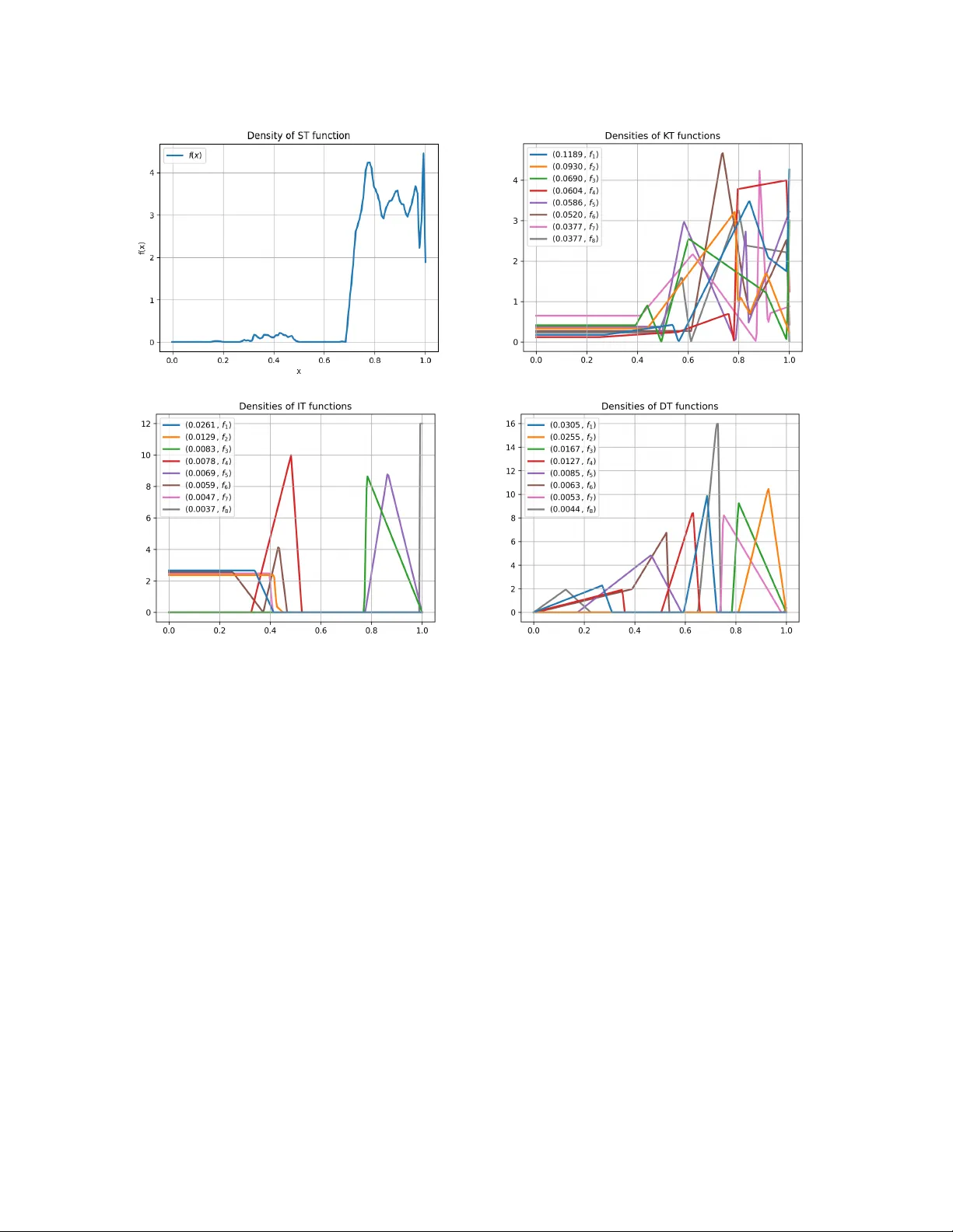
Impro v ed Appro ximation Algorithms for Multiw a y Cut b y Large Mixtures of New and Old Rounding Sc hemes ∗ Josh ua Brak ensiek † Neng Huang ‡ Aaron P otec hin § Uri Zwic k ¶ Abstract The input to the Multiw ay Cut problem is a weigh ted undirected graph, with nonnegative edge w eights, and k designated terminals. The goal is to partition the v ertices of the graph into k parts, each con taining exactly one of the terminals, suc h that the sum of weigh ts of the edges connecting v ertices in diﬀerent parts of the partition is minimized. The problem is APX-hard for k ≥ 3. The curren tly best kno wn appro ximation algorithm for the problem for arbitrary k , obtained by Sharma and V ondr´ ak [STOC 2014] more than a decade ago, has an approximation ratio of 1.2965. W e present an algorithm with an improv ed approximation ratio of 1.2787. Also, for small v alues of k ≥ 4 w e obtain the ﬁrst impro vemen ts in 25 years ov er the currently b est appro ximation ratios obtained by Karger, Klein, Stein, Thorup, and Y oung [STOC 1999]. (F or k = 3 an optimal approximation algorithm is known.) Our main technical contributions are new insights on rounding the LP relaxation of C˘ alinescu, Karloﬀ, and Rabani [STOC 1998], whose in tegralit y ratio matches Multiw ay Cut’s approx- imabilit y ratio, assuming the Unique Games Conjecture [Manok aran, Naor, Ragha vendra, and Sc hw artz, STOC 2008]. First, we introduce a generalized form of a rounding scheme suggested b y Klein b erg and T ardos [F OCS 1999] and use it to replace the Exponential Clo cks rounding sc heme used b y Buc h binder, Naor, and Sc h wartz [STOC 2013] and by Sharma and V ondr´ ak. Sec- ond, while previous algorithms use a mixture of tw o, three, or four basic rounding schemes, eac h from a diﬀerent family of rounding schemes, our algorithm uses a computationally-discov ered mixture of hundreds of basic rounding schemes, each parametrized by a random v ariable with a distinct probability distribution, including in particular man y diﬀeren t rounding schemes from the same family . W e give a completely rigorous analysis of our impro ved algorithms using a com bination of analytical techniques and in terv al arithmetic. ∗ F ull version of paper to app ear in the proceedings of STOC 2026. Companion co de: https://github.com/ jbrakensiek/multiway- cut- verification † Univ ersity of California, Berkeley . Email: josh.brakensiek@berkeley.edu . Supp orted in part b y a Simons In vestigator a ward and NSF gran ts CCF-2211972 and DMS-2503280. ‡ Univ ersity of Mic higan. Email: nengh@umich.edu § Univ ersity of Chicago. Email: potechin@uchicago.edu ¶ Bla v atnik School of Computer Science, T el Aviv Universit y , Israel. Email: zwick@tau.ac.il . W ork supported b y ISF grant 2735/2025. 1 In tro duction The input to the (Minimum) Multiwa y Cut problem is a w eighted undirected graph G = ( V , E , w ), where w : E → R + , with k designated v ertices called terminals . The ob jectiv e is to ﬁnd a partition of V into k parts, each containing exactly one terminal, so as to minimize the total weigh t of edges whose endp oints lie in diﬀerent parts of the partition. F or k = 2 this is the classical min s - t cut problem whic h admits eﬃcient p olynomial-time algorithms. F or k ≥ 3, how ever, the problem is APX-hard [ DJP + 94 ]. This motiv ated a long series of pap ers [ DJP + 94 , CKR00 , KKS + 04 , CCT06 , SV14 , BNS18 , BSW19 , BSW21 ] that design approximation algorithms for the problem, with grad- ually improving appro ximation ratios. The currently b est approximation algorithm for arbitrary k , due to Sharma and V ondr´ ak [ SV14 ], achiev es a ratio of 1 . 2965. F or the full history of the problem, and a summary of all previous results, see T able 1 and Section 1.1 . F or k = 3, Karger, Klein, Stein, Thorup, and Y oung [ KKS + 04 ] and indep enden tly Cheung, Cun- ningham, and T ang [ CT99 , CCT06 ], combined with a result of Manok aran, Naor, Raghav endra, and Sch w artz [ MNRS08 ], show ed that the b est approximation ratio for the problem, assuming the Unique Games Conjecture (UGC), is 12 11 = 1 . 0909 . . . . Karger et al. [ KKS + 04 ] also giv e impro ved appro ximation algorithms for small v alues of k . These results are summarized in T able 2 . Our main result is an impro ved approximation algorithm for the Multiw ay Cut problem, for arbi- trary k , whose appro ximation ratio is 1 . 2787. This is the ﬁrst improv ed appro ximation ratio for the problem for o ver a decade. Theorem 1.1. Multiway Cut with an arbitr ary numb er of terminals has a p olynomial-time 1 . 2787 - appr oximation algorithm. W e also obtain impro v ed approximation ratios for every v alue of k ≥ 4. F or the exact approximation ratios, see T able 2 . These are the ﬁrst improv emen ts of these appro ximation ratios for o ver 25 y ears. In particular, w e hav e: Theorem 1.2. (a) Multiway Cut with 4 terminals has a p olynomial-time 1 . 1489 -appr oximation al- gorithm. (b) Multiway Cut with 5 terminals has a p olynomial-time 1 . 1837 -appr oximation algorithm. (c) Multiway Cut with 6 terminals has a p olynomial-time 1 . 2149 -appr oximation algorithm. 1.1 Previous W ork Dahlhaus et al. [ DJP + 92 , DJP + 94 ] were the ﬁrst to consider the Multiw ay Cut problem from the computational complexity p ersp ective. They pro ved that the problem is APX-hard for k ≥ 3 and ga ve a simple com binatorial algorithm with an appro ximation ratio of 2 − 2 k . They also show ed that in planar graphs, the problem can b e solv ed in p olynomial time for ev ery ﬁxed k , but is NP-hard when k is part of the input. Cunningham [ Cun91 ], Chopra and Rao [ CR91 ], and Bertsimas, T eo, and V orha [ BTV99 ] studied the facets of the m ultiwa y cut polyhedron and suggested some simple linear programming relaxations of the problem. These did not lead to improv ed approximation ratios. The next ma jor step was made b y C˘ alinescu, Karloﬀ, and Rabani [ CKR00 ]. They introduced a stronger LP relaxation of the problem, equiv alent to em b edding the v ertices of the graph in to the k -simplex ∆ k = { ( u 1 , u 2 , . . . , u k ) | u 1 , u 2 , . . . , u k ≥ 0 , P k i =1 u i = 1 } , 1 and used a simple Single 1 According to our deﬁnition, the k -simplex has k vertices and is ( k − 1)-dimensional. Some authors refer to this as the ( k − 1)-simplex. Our notation seems more conv enient for our purposes. 1 Ratio P ap er Metho d Analysis T yp e 2 [ DJP + 94 ] Com binatorial Analytic 1.5 [ CKR00 ] ST Analytic 1.3438 [ KKS + 04 ] ST + IT Analytic 1.3239 [ BNS18 ] ST + EC/KT Analytic 1.3022 [ SV14 ] ST + EC/KT + DT Analytic 1.2970 [ BSW21 ] Simplex T rans. + ST + EC/KT Analytic 1.2965 [ SV14 ] ST + EC/KT + IT + DT Computational 1.2787 Here ST + GKT ∗ + IT ∗ + DT ∗ Computational T able 1: A summary of Multiwa y Cut approximation algorithms for an arbitrary num b er of termi- nals k . The “Metho d” column describ es the rounding tec hniques used by the algorithms according to the following legend: Single Threshold (ST), Indep endent Thresholds (IT), Exp onential Clo cks or Klein b erg-T ardos (EC/KT), Descending Thresholds (DT), and Generalized Kleinberg-T ardos (GKT). A star, as in IT ∗ , indicates that sev eral indep enden t copies of the rounding schemes of this families are used, eac h parametrized by a diﬀerent random v ariable. Thr eshold (ST) rounding scheme to obtain an appro ximation algorithm with an appro ximation ratio of 1 . 5 − 1 k . All subsequent approximation algorithms for the Multiwa y Cut problem use the relaxation of C˘ alinescu et al. [ CKR00 ]. F or completeness, the CKR LP relaxation is describ ed in App endix A . Karger et al. [ KKS + 99 , KKS + 04 ] obtained an improv ed appro ximation ratio of 1 . 3438. Their algorithm uses the Single Threshold (ST) rounding sc heme of C˘ alinescu et al. [ CKR00 ] together with another rounding sc heme which is now known as Indep endent Thr esholds (IT) . As mentioned, Cheung, Cunningham, and T ang [ CT99 , CCT06 ] and indep endently Karger et al. [ KKS + 99 , KKS + 04 ], obtained a 12 11 -appro ximation ratio for the case k = 3. They also show ed that this matc hes the integralit y ratio of the relaxation of C˘ alinescu et al. [ CKR00 ]. Karger et al. [ KKS + 99 , KKS + 04 ] also obtained improv ed approximation ratios for small v alues of k . F or k = 4 , 5, their b est algorithms are obtained b y discretizing the simplex and using v ery large linear programs to ﬁnd nearly-optimal distributions of side-p ar al lel cuts (sp ar cs) . F or k ≥ 6, they use their algorithm for general k with slightly tuned parameters. The exact ratios obtained can b e found in T able 2 . The next improv emen t, for general k , was obtained b y Buch binder, Naor, and Sch w artz [ BNS18 ]. They obtained a simple approximation algorithm with an appro ximation ratio of 4 3 − 4 9 k − 6 < 1 . 3334 and a slightly more complicated algorithm with an approximation ratio of 1 . 3239 − 1 24 k . Their algorithms use a mixture of the Single Threshold (ST) rounding sc heme with a non-uniform random v ariable, and a tec hnique called Exp onential Clo cks (EC) that w as previously introduced b y Ge, He, Y e, and Zhang [ GHYZ11 ]. They also show ed that the Exp onen tial-Clo c ks (EC) rounding sc heme could b e replaced b y a rounding scheme introduced by Kleinberg and T ardos [ KT02 ]. Sharma and V ondr´ ak [ SV14 ] built on the results of Buc h binder et al. [ BNS18 ] and obtained three impro ved approximation algorithms for the Multiw ay Cut problem. Their ﬁrst algorithm, with a ratio of 3+ √ 5 4 ≃ 1 . 309017, w as obtained using a combination of the Si ngle Thr eshold (ST) and Exp onen tial-Clo cks (EC) rounding tec hniques, as used b y Buc hbinder et al. [ BNS18 ]. They also 2 k SP ARCs [ KKS + 04 ] ST+IT [ KKS + 04 ] EC+ST [ BNS18 ] New Algorithms Lo wer Bound [ AMM17 ] 4 1.1539 1.189 1.2000 1.1489 1.125 5 1.2161 1.223 1.2308 1.1837 1.142 6 1.2714 1.244 1.2500 1.2149 1.1538 7 1.3200 1.258 1.2632 1.2399 1.1612 8 1.3322 1.269 1.2728 1.2499 1.1666 9 – 1.277 1.2800 1.2549 1.1707 10 – 1.284 1.2858 1.2599 1.1739 an y 1.2787 1.20016 [ BCKM20 ] T able 2: Upp er and lo wer b ounds on the approximation ratios of the Multiw ay Cut problem with k = 4 , 5 , . . . , 10 terminals. (F or k = 3 a tigh t b ound of 12 11 = 1 . 0909 ... is known.) The low er b ounds are on the integralit y ratio of the LP relaxation of Multiwa y Cut, which translate under the Unique Games Conjecture to low er b ounds on the approximabilit y ratio of the problem. The last line restates the appro ximation ratio that w e get for an arbitrary n umber of terminals and also gives the b est known lo wer bound for this case. The appro ximation ratio that w e obtain for general k impro ves ov er all previously known results for k ≥ 10. sho wed that under some mild assumptions, this is the b est ratio that can b e obtained b y com bining these t w o tec hniques. Their second approximation algorithm, with a ratio of 10+4 √ 3 13 ≃ 1 . 30217, w as obtained b y combining the tw o original rounding sc hemes with a new rounding technique which they call Desc ending Thr esholds (DT) . Their third and ﬁnal algorithm, with an appro ximation ratio of 1 . 2965, is obtained by adding the Indep endent Thresholds (IT) rounding technique of Karger et al. [ KKS + 04 ] to the mix. Their analysis of the third algorithm is computer assisted. Buc hbinder, Sch w artz, and W eizman [ BSW21 ] obtained a relatively simple algorithm with an ap- pro ximation ratio of 297 229 ≃ 1 . 29694, almost matching the b est appro ximation ratio of Sharma and V ondr´ ak [ SV14 ]. This is curren tly the b est appro ximation ratio that can b e v eriﬁed analytically without the use of a computer. Their algorithm uses an in teresting technique called simplex tr ans- formations . As a result, unlik e all algorithms discussed ab o ve, their algorithm uses cuts that are not parallel to one of the faces of the simplex, i.e., cuts that dep end on more than one co ordinate. Buc hbinder, Sch w artz, and W eizman [ BSW19 ] used a global linear transformation to obtain an appro ximation ratio of 11 8 = 1 . 375 using just the Single Threshold (ST) rounding tec hnique. Manok aran, Naor, Ragha vendra, and Sc hw artz [ MNRS08 ] sho wed that, under the Unique Games Conjecture (UGC) of Khot [ Kho02 ], the in tegrality ratio of the LP relaxation of C˘ alinescu et al. [ CKR00 ] is the b est approximation ratio that can b e obtained for the Multiw ay Cut problem in p olynomial time. Thus, eﬀorts for obtaining improv ed approximation algorithms for the problem should concen trate on ﬁnding b etter w ays of rounding solutions of this LP relaxation. In particular, no improv ed res ults can b e obtained by trying to use semideﬁnite programming (SDP) relaxations. F reund and Karloﬀ [ FK00 ] show ed that the integralit y ratio of the CKR relaxation is at least 8 / (7 + 1 k − 1 ), for any k ≥ 3. Angelidakis, Mak aryc hev, and Manurangsi [ AMM17 ] improv ed the lo wer b ounds to 6 / (5 + 1 k − 1 ) by in tro ducing an interesting new framew ork of non-opp osite cuts . B ´ erczi, Chandrasek aran, Kir´ aly , and Madan [ BCKM20 ] used this framework to obtain a lo wer b ound of 1 . 20016 for general k . 3 1.2 Our Con tributions and T ec hniques Our improv ed appro ximation algorithms for Multiw ay Cut are obtained by designing impro v ed rounding schemes for the LP relaxation of C˘ alinescu et al. [ CKR00 ]. Previous algorithms used a mixture of up to four basic rounding schemes, each taken from a diﬀeren t family of rounding sc hemes. As mentioned the families of rounding sc hemes used w ere: Single Threshold (ST), In- dep enden t Thresholds (IT), Exp onential clo cks (EC) or Kleinberg-T ardos (KT), and Descending Thresholds (DT). W e improv e on all previous results using the follo wing steps: 1. W e introduce a generalized version of the Kleinberg-T ardos (KT) rounding sc heme. 2. W e use man y basic rounding sc hemes from eac h family of rounding schemes, eac h parametrized b y a random v ariable with a diﬀerent distribution. 3. W e devise an algorithm for ﬁnding go o d mixtures of a v ery large num b er of basic rounding sc hemes b y approximating the solution of an inﬁnite 0-sum game play ed by a cut play er and an edge pla yer. 4. W e use rigorous computational techniques, in particular Interval Arithmetic , to obtain rigor- ous computer-assisted pro ofs of the appro ximation ratios obtained. W e elab orate on each of these steps in the following sections. 1.2.1 Generalized Kleinberg-T ardos A (multiw ay) cut of the k -simplex ∆ k = { ( u 1 , u 2 , . . . , u k ) | u 1 , u 2 , . . . , u k ≥ 0 , P k i =1 u i = 1 } is a function c : ∆ k → [ k ] that maps each point of the simplex to one of the k terminals, suc h that c ( e i ) = i , for i ∈ [ k ], i.e., the i -th v ertex of the simplex is mapp ed to terminal i . A r ounding scheme is a probabilit y distribution ov er cuts. Klein b erg and T ardos [ KT02 ] introduced the following rounding scheme, whic h we call KT, and used it to obtain a 2-approximation algorithm for the Uniform Metric Labeling problem. Initially all the simplex p oin ts are unassigned. The rounding scheme pro ceeds in rounds. In eac h round, a uniformly random terminal i ∈ [ k ] and a uniformly random thr eshold t ∈ [0 , 1] are c hosen. Each unassigned simplex point u = ( u 1 , u 2 , . . . , u k ) with u i ≥ t is assigned to terminal i , i.e., c ( u ) = i . This pro ceeds un til all simplex p oin ts are assigned. This rounding scheme, unlike all other sc hemes w e consider, samples the terminals with r ep etitions . It is not diﬃcult to chec k that the exp ected n umber of rounds needed to ‘color’ the whole simplex is p olynomial in k . Buc hbinder, Naor, and Sc hw artz [ BNS18 ] sho wed that the rounding tec hnique of Kleinberg and T ardos [ KT02 ] can b e used to replace the Exponential Clocks (EC) rounding tec hnique whic h they and Sharma and V ondr´ ak [ SV14 ] use in their approximation algorithms, as b oth rounding tec hniques, although very diﬀerent from each other, ha ve iden tical cut density functions, as we deﬁne b elo w. (F or a more formal deﬁnition, see Section 2 .) A Generalized Klein b erg-T ardos (GKT) rounding sc heme is a rounding sc heme in whic h the random thresholds are chosen nonuniformly . More precisely , w e let KT( f ), where f : [0 , 1] → R + is a density function, b e the Generalized Kleinberg-T ardos rounding sc heme in which the random thresholds are chosen indep enden tly according to a random v ariable with densit y function f . T o ensure termination w e require that F ( 1 k ) > 0, where F ( x ) = R x 0 f ( t ) dt is the cumulativ e probabilit y 4 function corresp onding to f . It is interesting to note that while non uniform thresholds were used in conjunction with man y of the other random tec hniques, this was not tried with the Klein b erg-T ardos rounding scheme. Our results show that c ho osing the thresholds nonuniformly greatly enhances the p erformance of suc h rounding schemes. If R is a rounding sc heme and u , v ∈ ∆ k are tw o simplex p oints, we let P R k ( u , v ) = P [ c ( u )  = c ( v )] b e the probabilit y that the edge ( u , v ) is cut by the rounding sc heme R . If R is symmetric , i.e., it treats all terminals equally 2 , w e can restrict our attention to (1 , 2) -aligne d e dges , i.e., edges of the form u = ( u 1 , u 2 , . . . , u k ) and v = u − ε ( e 1 − e 2 ) = ( u 1 − ε, u 2 + ε, u 3 , . . . , u k ). W e deﬁne the density of the rounding sc heme R at u as follo ws: d R k ( u ) = lim ε → 0 P R k ( u , u − ε ( e 1 − e 2 )) ε . It is known that sup u ∈ ∆ k d R k ( u ) is the appro ximation ratio achiev ed by using the rounding scheme R . One of the features that mak e the Klein b erg-T ardos (KT) and the Exp onential Clocks (EC) round- ing sc hemes attractiv e is that they hav e v ery simple densit y functions d KT k ( u ) = d EC k ( u ) = 2 − u 1 − u 2 . Used on their own, each one of these rounding sc hemes only gives an appro xima- tion ratio of 2 for the Multiwa y Cut problem. How ev er, they are useful in combination with other rounding tec hniques. As a ﬁrst step tow ards using Generalized Klein b erg-T ardos schemes KT( f ) to obtain impro v ed appro ximation algorithms, we obtain the following relatively simple form ula for their densities: Prop osition 1.3 (See Corollary 2.4 ) . L et f : [0 , 1] → R + b e a pr ob ability density function and let F : [0 , 1] → [0 , 1] b e its c orr esp onding cumulative density function. Then, d KT( f ) k ( u 1 , u 2 , . . . , u k ) = f ( u 1 ) P k i =1 F ( u i ) 1 − F ( u 1 ) P k i =1 F ( u i ) ! + f ( u 2 ) P k i =1 F ( u i ) 1 − F ( u 2 ) P k i =1 F ( u i ) ! . Note that if f ( x ) = 1 and F ( x ) = x , the density simpliﬁes to 2 − u 1 − u 2 . By v arying the distribution f ov er [0 , 1], w e get access to a large family of cut density functions that w ere not a v ailable to prior approac hes to Multiw ay Cut. How ev er, to tak e adv an tage of this newfound freedom, w e also need a no v el approach to discov ering mixtur es of rounding sc hemes with a lo w approximation ratio, as discussed b elow. A p ossible alternativ e approac h is to consider generalized versions of the Exp onen tial Clo cks (EC) rounding technique in whic h a distribution other than the exp onential distribution is used for the ‘clo c ks’. W e discuss this option brieﬂy in App endix C . The main diﬃcult y with this approach is that the corresp onding densit y functions seem hard to work with. 1.2.2 Using Large Mixtures of Rounding Sc hemes If R 1 , R 2 , . . . , R n are rounding sc hemes, and ( p 1 , p 2 , . . . , p n ) ∈ ∆ n , the mixtur e R = P n i =1 p i R i is the rounding scheme that applies R i with probability p i , for i ∈ [ n ]. W e refer to the R i ’s as the b asic rounding schemes that constitute R . By the linearity of exp ectations, w e ha ve d R k ( u ) = P n i =1 p i d R i k ( u ). Mixtures allow an algorithm designer to balance out sev eral rounding sc hemes whose densities are maximized at diﬀeren t p oints of the k -simplex. 2 More sp eciﬁcally , P R k ( u , v ) is inv arian t under p ermutation of terminals. All rounding sc hemes considered in this pap er are symmetric. In fact, one can show that any rounding scheme can b e replaced with a symmetric one without increasing the w orst-case cut density . 5 As men tioned ab o v e, most approximation algorithms for Multiw ay Cut use a mixture of several basic rounding sc hemes, each tak en from a diﬀerent family of rounding sc hemes. Sharma and V ondr´ ak [ SV14 ], for example, use a mixture of four basic rounding schemes, ST( f ), EC/KT, IT( g ), and DT( g ), where f is a rather complicated, computationally discov ered, densit y function and g is the densit y function of a uniformly random v ariable on [0 , 6 11 ]. (See the legend giv en in T able 1 and Section 2 .) W e note that with the exception of Single Threshold (ST), the other families of rounding schemes, including the newly in tro duced family KT( f ) of generalized Klein b erg-T ardos rounding schemes, are nonline ar , in the sense that α 1 KT( f 1 ) + α 2 KT( f 2 )  = KT( α 1 f 1 + α 2 f 2 ). In fact, α 1 KT( f 1 ) + α 2 KT( f 2 ) do es not seem to b e equiv alen t to KT( g ) for any density function g . The same observ ation holds also for Indep enden t Thresholds (IT) and Descending Thresholds (DT). As a conse quence, it ma y b e b eneﬁcial to use a mixture that contains man y rounding sc hemes from eac h family of rounding schemes, eac h with its distinct density function. Thus, for example, we ma y use a mixture that con tains KT( f 1 ), KT( f 2 ),. . . , KT( f n ), for an arbitrarily large v alue of n , and similarly IT( g 1 ), IT( g 2 ),. . . , IT( g m ), etc. Our results sho w that using such large mixtures is indeed b eneﬁcial and ma y lead to substantially improv ed approximation ratios. This observ ation substantially broadens the range of possibilities. Exploring this huge space man- ually seems practically imp ossible. W e thus need an automated tec hnique for discov ering go o d mixtures of rounding sc hemes, mixtures that could p ossibly contain h undreds of basic rounding sc hemes. 1.2.3 Computational Discov ery of Rounding Sc hemes Computational techniques were used in several of the previous pap ers on the Multiwa y Cut problem. Both Cheung et al. [ CT99 , CCT06 ] and Karger et al. [ KKS + 04 ] solv ed large linear programs, obtained b y discretizing the 3-simplex, to disco ver similar, but not identical, optimal algorithms for k = 3 and to obtain matching low er b ounds on the in tegrality ratio of the relaxation. Once the optimal algorithms were disco vered, they were able to analyze them without the use of a computer. Karger et al. [ KKS + 04 ] also used tw o diﬀeren t computational approac hes to obtain their algorithms for k ≥ 4. F or k = 4 , 5 they again solv ed large linear programs, somewhat diﬀeren t from the ones used for k = 3, to obtain their b est algorithms for these v alues. F or k ≥ 6 they obtained their b est algorithms using a mixture of ST( f ) and IT( g ), where f is the density function of a uniform random v ariable on [ b, 1], and g is the densit y of a uniform random v ariable on [0 , b ], where b ∈ [0 , 1] is a parameter that they tuned computationally . (F or eac h v alue of k they use a diﬀeren t v alue of b .) Sharma and V ondr´ ak [ SV14 ] used a mixture of ST( f ), EC/KT, IT( g ) and DT( g ), where f is a complicated densit y function discov ered computationally and g is the density function of a uniformly random v ariable on [0 , 6 11 ]. Because of the linearity of the densit y function of ST schemes, they w ere able to solv e a h uge linear program that optimizes a very ﬁne discrete v ersion of f , and the probabilities with whic h each one of their four basic rounding schemes should b e used. W e use m uch more extensiv e computational tec hniques to disco ver rounding sc hemes that are mix- tures of hundreds of basic rounding sc hemes, eac h with its own densit y function. This in volv es solving many nonlinear, and non-con vex, optimization problems. W e do that using standard nu - merical optimization tec hniques. (More details are given in Section 4 .) These tec hniques are, 6 of course, not guaranteed to ﬁnd globally optimal solutions. Ho wev er, once we get a suggested rounding sc heme, we can rigorously obtain an upp er b ound on its approximation ratio. W e next give a high-lev el description of our computational techniques. Let R 1 , R 2 , . . . , R n b e a ﬁnite collection of rounding schemes and let u 1 , u 2 , . . . , u m b e a ﬁnite collection of simplex p oin ts. W e can use a linear program to ﬁnd a mixture R = P n i =1 p i R i of the rounding sc hemes that minimizes max j ∈ [ m ] d R k ( u j ). The dual linear program ﬁnds a distribution ( q 1 , q 2 , . . . , q m ) o ver the a v ailable simplex p oints that maximizes min i ∈ [ n ] P m j =1 q j d R i k ( u j ). This can th us b e view ed as a 0 -sum game , with pay oﬀ matrix ( d R i k ( u j )), play ed b etw een the algorithm designer, who c ho oses rounding sc hemes, and the adversary , who c ho oses simplex p oints. View ed from this p ersp ective, it is not surprising that in most cases, the optimal strategies of the tw o play ers are mixe d , i.e., a probabilit y distribution ov er either the rounding sc hemes or the simplex p oints. Suc h linear programs w ere used by many of the previous pap ers, including [ CT99 , CCT06 , KKS + 04 , SV14 ]. W e go one step further. Supp ose that ( p 1 , p 2 , . . . , p n ) and ( q 1 , q 2 , . . . , q m ) are the optimal mixed strategies of the pla yers in the abov e game. W e try to ﬁnd a new rounding sc heme R ′ for which P m j =1 q j d R ′ k ( u j ) is smaller than the v alue of the game and add R ′ to the collection of basic rounding sc hemes a v ailable to the algorithm designer. Similarly , w e also try to ﬁnd a new simplex p oin t u ′ for which d R k ( u ′ ) = P n i =1 p i d R i k ( u ′ ) is larger than the v alue of the game and add it to the collection of simplex p oints. After eac h such step w e resolv e the 0-sum game and obtain the newly optimal distributions. W e let this process run for as long as we c an, or until no signiﬁcantly improv ed results are found. F or more details, see Section 4 . W e note that a similar computational tec hnique w as used by Brak ensiek, Huang, Potec hin, and Zwic k [ BHPZ23 ] to disco v er impro v ed appro ximation algorithms for MAX DI-CUT and other MAX CSP problems. 1.2.4 V eriﬁcation Using In terv al Arithmetic An interv al arithmetic system pro vides functions for computing the basic arithmetic op erations, and other basic functions such as exp( x ), on intervals rather than on num b ers. The functions return an interv al that is guaranteed to contain the correct interv al. F or example, if f int is an in terv al arithmetic implementation of a function f , and I = [ a, b ] is an interv al, then f int ( I ) ⊇ f ( I ) = { f ( x ) | x ∈ I } . Note that f int is not required to return f ( I ) exactly , as it may b e imp ossible to represent the true endp oints of the interv al using the mac hine precision, or it ma y b e to o time consuming to compute them exactly . T o b e useful, ho wev er, f int ( I ) should not b e m uch larger than f ( I ). By combining the in terv al implementations of the basic functions, in terv al implemen tation of muc h more complicated functions can b e obtained. It is imp ortant to note that the in terv al implemen tation of the basic functions should take into accoun t all numerical errors, including ﬂoating p oint rounding errors, that may o ccur during the computation of the ﬁnal interv al. W e make use of a mo dern interv al arithmetic library called Arb [ Joh17 , Joh19 ]. T o illustrate the usefulness of interv al arithmetic, consider the follo wing example. Supp ose that f ( x 1 , x 2 , . . . , x k ) is a con tin uous, and p ossibly diﬀeren tiable, function deﬁned on [0 , 1] k . Supp ose that m = min x 1 ,...,x k ∈ [0 , 1] f ( x 1 , x 2 , . . . , x k ) and that m > 0. Our goal is to prov e that m > 0. A traditional approach is to compute the partial deriv atives of f , assuming that f is diﬀeren tiable, lo ok for critical p oints and sho w that f is positive at all critical p oin ts. This is actually not enough as we also need to lo ok for critical points on the b oundary of the region. In many cases this approach is not feasible as the partial deriv ativ es may b e very complicated and there may 7 b e an enormous num b er of critical p oints. If w e can show that f ( x 1 , x 2 , . . . , x k ) is L -Lipschitz, i.e., | f ( x ) − f ( y ) | ≤ L ∥ x − y ∥ 1 , for every x , y ∈ [0 , 1] k , then in order to obtain the worst-case cut density within an y given additive error ϵ > 0, it is enough to ev aluate f on all p oints of the form ( i 1 N , i 2 N , . . . , i k N ), where i 1 , i 2 , . . . , i k ∈ { 0 , 1 , . . . , N } , for a suﬃciently large in teger N = N ( ϵ, L ). Ho wev er, this requires a rigorous b ound on the Lipschitz constan t L , and rigorous b ounds on the n umerical errors that could o ccur during all these function ev aluations, again not a pleasant task. Using interv al arithmetic, on the other hand, w e can adaptiv ely partition [0 , 1] k in to a collection of b o xes I 1 × I 2 × · · · × I k and compute f int ( I 1 , I 2 . . . , I k ) for eac h one of these b oxes. If all returned in terv als are p ositive, we get a rigorous proof that m > 0. In particular, this approac h neither requires that f is diﬀerentiable nor that w e hav e an explicit b ound on the Lipschitz constan t L . F urthermore, an y numerical errors are automatically accounted for b y the interv al arithmetic system. In terv al arithmetic was used b efore to obtain rigorous pro ofs of appro ximation ratios. (See, e.g., [ Zwi02 , Sj¨ o09 , ABG16 , BKK + 18 , BK20 , BHPZ23 , BHZ24 ].) W e note that Sharma and V ondr´ ak [ SV14 ] used computational techniques to obtain a b ound of 1 . 2965 on the approxima- tion ratio of their algorithm, but did not explicitly bound the numerical errors that may hav e o ccurred during the computation of this constant. (It is extremely unlik ely , ho wev er, that these una voidable n umerical errors aﬀect the fourth decimal digit of their bound.) The same holds for some of the b ounds obtained b y Karger et al. [ KKS + 04 ] for small v alues of k . Since our rounding sc hemes use mixtures of h undreds of basic rounding sc hemes, analyzing their p erformance b y hand is infeasible. W e therefore resort to in terv al arithmetic to rigorously b ound their p erformance ratios. F or small v alues of k we could in principle try to use the general approac h outlined abov e, with the k -dimensional b ox [0 , 1] k replaced b y the k -simplex ∆ k . Ho wev er, ev en for relativ ely small v alues of k this becomes infeasible and we need to use additional ideas. The basic approac h fails completely when k is arbitrary , as then we are essentially trying to minimize a function deﬁned on ∪ k ≥ 3 ∆ k . T o ov ercome these obstacles, our veriﬁcation works with pr eﬁxes of simplex p oints instead of simplex p oin ts themselves. A preﬁx of a simplex p oint is a tuple u = ( u 1 , . . . , u ℓ ) where 0 ≤ u 1 , . . . , u ℓ ≤ 1 and P ℓ i =1 u i ≤ 1. Such a preﬁx can b e extended to a point in the k -simplex, for an y k > ℓ , by app ending additional co ordinates u ℓ +1 , . . . , u k , making sure that P k i =1 u i = 1. (If P ℓ i =1 u i = 1, then u is already a simplex p oin t.) The density of a preﬁx u is deﬁned to b e the maxim um density of any simplex p oin t that can b e obtained b y extending u . The main purp ose of working with preﬁxes is that w e may use one ev aluation, namely , ev aluation of the density of the preﬁx, to co ver all simplex p oin ts ha ving that preﬁx. Bounding densities of preﬁxes is a nontrivial task. Karger et al. [ KKS + 04 ] and Sharma and V ondr´ ak [ SV14 ] used a similar approach in their analytical and computational analyses, but only with preﬁxes of length ℓ = 2. T o get our improv ed appro ximation ratios w e need to consider longer preﬁxes. The main tec hnical diﬃculty now is to obtain a go o d upp er b ound on the density of preﬁxes of an y length. It turns out that b y imp osing v ery mild conditions on our rounding schemes, w e can deriv e a tight upp er b ound on the density of not all, but a sizable c h unk of simplex p oints having the preﬁx. More sp eciﬁcally , if w e assume that in our mixture R , there e xists some α > 0 such that for any IT( f ) ∈ R , f is increasing on [0 , α ], and for an y KT( g ) ∈ R , g is constan t on [0 , α ], then w e may deﬁne a function d R for ev ery R ∈ R such that for any preﬁx u = ( u 1 , . . . , u ℓ ) and k ≥ ℓ , 8 max 0 ≤ u ℓ +1 ,...,u k ≤ α P k i =1 u i =1 d R k ( u 1 , u 2 , . . . , u ℓ , u ℓ +1 , . . . , u k ) ≤ d R ( u ) . (1) F urthermore, equalit y is ac hiev ed most of the time (See Lemmas 6.2 and 6.8 for more details). The ev aluation for the expression on the right hand side is straigh tforward for ST, GKT, and DT sc hemes. F or IT schemes it is more complicated, for we need to derive an expression in volving Kummer’s conﬂuen t hypergeometric function (see Lemma 3.7 ). This leads naturally to our v eriﬁcation algorithm, for whic h w e no w give a high-lev el description. Let us say w e are attempting to v erify that the density ac hieved by R (which satisﬁes the abov e conditions regarding IT and GKT sc hemes) is alw ays at most d 0 for some d 0 > 0. Using interv al arithmetic, we work with sets of preﬁxes U = U 1 × · · · × U ℓ , where U 1 , . . . , U ℓ are interv als within [0 , 1]. W e implement in in terv al arithmetic the ev aluation of E R ∈R [ d R ( U )], which giv es us an in terv al con taining ev aluations of E R ∈R [ d R ( u )] for preﬁxes u ∈ U . If we ﬁnd some u ∈ U for this ev aluation is greater than d 0 , then w e get a preﬁx whic h could p oten tially be extended to a p oint on which the density of R is greater than d 0 (in fact, it can in most cases). In this c ase we halt the v eriﬁcation without success. Otherwise, by ( 1 ) we kno w that for every simplex p oint with preﬁx in U whose remaining co ordinates are all at most α , its cut densit y is at most d 0 . So we consider this lev el “passed”, and add a new in terv al U ℓ +1 = [ α, 1] and recursiv ely apply this algorithm. Since the coordinates of an y simplex point sum to 1, w e can add at most 1 /α new co ordinates, which guaran tees that the veriﬁcation will terminate in a ﬁnite amoun t of time. This strategy may also b e adapted for v eriﬁcation of a ﬁnite ﬁxed k . See Section 6 for more details. 1.3 Related W ork The Multiwa y Cut problem is a sp ecial case of the 0-Extension problem, introduced b y Karzanov [ Kar98 ], and the Metric L ab eling problem introduced by Kleib ert and T ardos [ KT02 ]. In the 0- Extension problem, in addition to the weigh ted undirected graph G = ( V , E , w ), where w : E → R + , the input also includes a metric d deﬁned on the set of terminals T . T o goal is to ﬁnd an assignmen t ℓ : V → T that minimizes the separation cost P { u,v }∈ E w ( u, v ) d ( ℓ ( u ) , ℓ ( v )). If d is the uniform metric, i.e., d ( t, t ′ ) = 1, if t  = t ′ , and d ( t, t ) = 0, this is exactly the Multiw ay Cut problem. In the Metric Lab eling problem, the input also includes an assignment c ost function c : V × T → R + and the goal is to ﬁnd an assignment ℓ : V → T that minimizes P u ∈ V c ( u, ℓ ( u )) + P { u,v }∈ E w ( u, v ) d ( ℓ ( u ) , ℓ ( v )), the sum of the assignmen t and separation costs. A sp ecial case of the Metric Labeling problem that still captures the Multiwa y Cut problem is the Uniform Metric L ab eling problem in whic h the metric d is the uniform metric. The b est approximation ratio kno wn for the 0-Extension problem is O (log k / log log k ) [ CKR05 , FHR T03 ], where k = | T | is the num b er of terminals. The b est approximation ratio known for the Metric Lab eling problem is O (log k ) [ KT02 ]. The b est approximation ratio known for the Uniform Metric Lab eling problem is 2 [ KT02 ]. Manok aran et al. [ MNRS08 ] show ed that, under the Unique Games Conjecture (UGC), the b est appro ximation ratios that can b e obtained for the 0-Extension and the Metric Lab eling problems in p olynomial time are equal to the intergalit y ratios of the e arth mover LP relaxations of these problems in tro duced by Chekuri, Khanna, Naor, and Zosin [ CKNZ04 ]. A complementary problem to Multiw a y Cut is Multiway Uncut , where one seeks to maximize the n umber (or total weigh t) of edges which are not cut by an assignment to the terminals. The exact 9 optimization problem is equiv alent to Multiwa y Cut, but the quantitativ e guarantees of approxi- mation algorithms are rather diﬀerent. Langb erg, Rabani, and Swam y [ LRS06 ] studied Multiwa y Uncut and obtained an approximation ratio of 0 . 8535, with a nearly matching LP in tegrality gap of 6 7 ≈ 0 . 8571. Ene, V ondr´ ak, and W u [ EVW13 ] studied a n umber of generalizations of Multiw ay Cut. The authors divided these generalizations into t wo categories (1) submo dular optimization problems general- ization Multiwa y Cut (Submo dular Multiwa y Parition) and (2) Min-CSP problems generalizing Multiw ay Cut (e.g., Hyp er gr aph Multiwa y Cut). In b oth cases, they show ed that in general the optimal appro ximation ratio is 2 − 2 k assuming either RP  = N P or the Unique Games Conjecture. They also obtained b etter appro ximation ratios in some sp ecial cases. V ery recently , B´ e rczi, Kir´ aly , and Szab o [ BKS24 ] p osed a v arient of Multiw ay Cut where the k terminals are not ﬁxed, but rather the i th terminal can b e chosen from a subset S i of the vertices pro vided as part of the input. They study the existence (or non-existence) of approximation algo- rithms for many v ersions of this question. Of note, a num ber of their appro ximation algorithms use an optimal appro ximation algorithm for Multiwa y Cut as a black-box. In particular, Theorem 1.1 automatically impro ves the quantitativ e guarantees of many of their algorithms. Eﬀort has also b een put into solving Multiw ay Cut exactly for sp ecial families of graphs. As previ- ously men tioned, Dahlhaus et al. [ DJP + 92 , DJP + 94 ] sho wed that Multiwa y Cut can b e eﬃciently solv ed for the class of planar graphs. More recently , Hirai [ Hir18 ] dev elop ed a theory of submodular optimization on a rather general set of lattices, showing as a corollary that problems like Multiwa y Cut and 0-Extension can b e solv ed exactly on “orientable mo dular” graphs. A notable op en question related to Multiwa y Cut is that of kernelization , where one seeks to eﬃcien tly replace the input (unw eighted) graph with a small graph such that (1) all k terminals are preserv ed in the smaller graph and (2) the optimal Multiw a y Cut in b oth graphs is identical. A natural target for the size of the k ernel is the sums of de gr e es D of the terminals as one can alw ays ﬁnd a multiw a y cut using at most D edges. 3 Kratsc h and W ahlstr¨ om [ KW20 ] can eﬃciently construct via a randomized algorithm a k ernel of size O ( D k +1 ), which is p olynomial for ﬁxed k . F or general k , recent work b y W ahlstr¨ om [ W ah22 ] pro ved that one can eﬃcien tly construct such a kernel of quasip olynomial size 2 O (log 4 D ) also via a randomized algorithm. See also the follo w-up w ork of W ahlstr¨ om [ W ah24 ] whic h constructs kernels for v arian ts of Multiwa y Cut. 1.4 Organization The rest of the pap er is organized as follo ws. In the next section w e deﬁne the basic families of rounding schemes used in the paper, including the new family of Generalized Klein b erg-T ardos (GKT) rounding sc hemes, and analyze each one of them. The analysis of GKT is no vel to the b est of our knowledge. W e also extend the analysis previously giv en for some of the other rounding sc hemes. In Section 3 w e obtain b ounds on the density functions of the GKT and IT rounding sc hemes when only a preﬁx of a simplex p oin t is given. (See the discussion in Section 1.2.4 .) In Section 4 we discuss the pro cess w e used for the discov ery of large mixtures of rounding schemes. In Section 5 we describ e the main features of the newly discov ered rounding sc hemes. In Section 6 w e consider the rigorous veriﬁcation of the approximation ratios claimed. In Section 7 , we discuss ho w our new results relate to the quest of ﬁnding truly optimal rounding schemes for Multiw ay Cut. W e end in Section 8 with some concluding remarks and op en problems. F urther material app ears in app endices. 3 Man y works in this ﬁeld use s instead of (our) k and k instead of (our) D . 10 2 Rounding Sc hemes and Their Analysis In this section we describ e the diﬀeren t rounding s c hemes used b y our algorithms. W e start with some general deﬁnitions and observ ations that apply to all schemes and then consider each scheme separately . All the rounding sc hemes R considered in the pap er, except for Exp onential Clo cks (EC) which is discussed brieﬂy , are of the following form. The sc heme chooses a random sequence σ (1) , σ (2) , . . . of terminals and a random sequence t 1 , t 2 , . . . of thr esholds . In the i -th round, the scheme assigns all yet unassigned simplex p oints ( u 1 , u 2 , . . . , u k ) with u σ ( i ) ≥ t i to terminal σ ( i ). The schemes diﬀer in the w a y the random sequences of terminals and thresholds are c hosen. In most sc hemes σ (1) , σ (2) , . . . , σ ( k ) is actually a p erm utation and t k = 0. That means that all simplex p oints that are y et unassigned at the b eginning of the k -th round are assigned to the ‘default’ terminal σ ( k ). Deﬁnition 2.1 (Cut probabilities) . F or a r ounding scheme R , L et P R k,ε ( u 1 , u 2 , . . . , u k ) b e the pr ob ability that the (1 , 2) -aligne d e dge of length ε c onne cting ( u 1 , u 2 , . . . , u k ) and ( u 1 − ε, u 2 + ε, . . . , u k ) is cut by R , i.e., the two endp oints of the e dge ar e assigne d by R to diﬀer ent terminals. L et P R, 1 k,ε ( u 1 , u 2 , . . . , u k ) b e the pr ob ability that ( u 1 , u 2 , . . . , u k ) is assigne d by R to terminal 1 and that ( u 1 − ε, u 2 + ε, . . . , u k ) is assigne d, at a later stage, to a diﬀer ent terminal. L et P R, 2 k,ε ( u 1 , u 2 , . . . , u k ) b e the pr ob ability that ( u 1 − ε, u 2 + ε, . . . , u k ) is assigne d by R to terminal 2 and that ( u 1 , u 2 , . . . , u k ) is assigne d, at a later stage, to a diﬀer ent terminal. F or all rounding schemes R considered in this pap er we ha ve: P R k,ε ( u 1 , u 2 , . . . , u k ) = P R, 1 k,ε ( u 1 , u 2 , . . . , u k ) + P R, 2 k,ε ( u 1 , u 2 , . . . , u k ) . This is b ecause if ( u 1 , u 2 , . . . , u k ) and ( u 1 − ε, u 2 + ε, . . . , u k ) are still unassigned, they can only b e assigned together to terminals other than 1 and 2. In other w ords, only terminals 1 or 2 can cut a (1 , 2)-aligned edge. The ‘later stage’ requirement is added to ensure that the even t in which ( u 1 , u 2 , . . . , u k ) is assigned to terminal 1 and ( u 1 − ε, u 2 + ε, . . . , u k ) is assigned to terminal 2 is not coun ted t wice. This subtlety is imp ortan t only for the Generalized Kleiberg-T ardos sc hemes (GKT). Note also that b y the symmetry of our rounding schemes we ha ve that P R, 2 k,ε ( u 1 , u 2 , . . . , u k ) = P R, 1 k,ε ( u 2 + ε, u 1 − ε, . . . , u k ) , and that P R k,ε ( u 1 , u 2 , . . . , u k ) is symmetric in u 3 , . . . , u k , i.e., it do es not dep end on the order of these argumen ts. Deﬁnition 2.2 (Cut densities) . d R k ( u 1 , . . . , u k ) = lim ε → 0 P R k,ε ( u 1 , u 2 , . . . , u k ) ε , d R,i k ( u 1 , . . . , u k ) = lim ε → 0 P R,i k,ε ( u 1 , u 2 , . . . , u k ) ε . As b efore, w e hav e: d R k ( u 1 , u 2 , . . . , u k ) = d R, 1 k ( u 1 , u 2 , . . . , u k ) + d R, 2 k ( u 1 , u 2 , . . . , u k ) . 11 If d R, 1 k ( u 2 , u 1 , . . . , u k ) is con tinuous, which holds for most of the schemes w e consider, then: d R, 2 k ( u 1 , u 2 , . . . , u k ) = d R, 1 k ( u 2 , u 1 , . . . , u k ) . Th us, to compute the cut density d R k ( u 1 , u 2 , . . . , u k ) of a scheme R we can concen trate on computing d R, 1 k ( u 1 , u 2 , . . . , u k ) and a corresp onding form ula for d R, 2 k ( u 1 , u 2 , . . . , u k ) w ould follow. All the rounding schemes w e use are parametrized by a con tinuous random v ariable T assuming v alues in [0 , 1]. 4 W e let f : [0 , 1] → [0 , ∞ ) be the density function (p df ) of this random v ariable, and F ( x ) = R x 0 f ( t ) dt b e the corresp onding cumulativ e distribution function (cdf ). Th us P [ T ≤ t ] = F ( t ). W e also let F ( u 1 , u 2 ) = F ( u 2 ) − F ( u 1 ), for u 1 ≤ u 2 , so that P [ t 1 < T ≤ t 2 ] = F ( t 1 , t 2 ). W e next consider the individual rounding sc hemes used, starting with the newly in tro duced gen- eralized version of the Kleinberg-T ardos rounding sch eme. W e next consider the Indep endent Thresholds (IT) rounding sc heme whic h was considered b efore but for which w e need to introduce a more delicate analysis. Finally , we consider the Single Threshold (ST) and Descending Thresholds (DT) rounding sc hemes. 2.1 Generalized Klein b erg-T ardos (GKT) Klein b erg and T ardos [ KT02 ] introduced their rounding scheme to obtain a 2-appro ximation al- gorithm for the uniform metric lab eling problem. It uses the uniform random v ariable on [0 , 1]. Buc hbinder, Naor, and Sch w artz [ BNS18 ] show ed that it is equiv alen t to their Exp onential Clo cks (EC) rounding sc heme. Interestingly , none of the previous papers on the Multiw ay Cut problem considered using the rounding scheme of Kleinberg and T ardos with a non-uniform random v ari- able, even though non-uniform random v ariables w ere used in all other rounding schemes. W e sho w that using the rounding scheme of Kleinberg and T ardos with a non-uniform random v ariable can lead to signiﬁcan tly improv ed approximation ratios for the Multiwa y Cut problem. A Generalized Kleinberg-T ardos scheme KT( f ), where f is a density function of a contin uous ran- dom v ariable with v alues in [0 , 1], w orks as follo ws. It rep eatedly chooses a terminal i ∈ [ k ] uniformly at random, and a random threshold t chosen according to the density function f , independent of all previous c hoices. If a simplex p oint u = ( u 1 , . . . , u k ) is y et unassigned and u i ≥ t then u is assigned to terminal i . This go es on until all simplex p oin ts, or until all simplex p oints that app ear in the em b edding of the input graph into the simplex, are assigned to terminals. T o ensure the termination of KT( f ) we require that F ( 1 k ) > 0 (since for an y simplex p oin t u = ( u 1 , . . . , u k ), there exists some i ∈ [ k ] such that u i ≥ 1 /k ). KT( f ) diﬀers from all other rounding sc hemes considered in this pap er in that it do es not choose a random p erm utation of the terminals. Instead, it samples terminals with rep etitions. W e next provide an analysis of KT( f ) generalizing the analysis of [ KT02 ] and [ BNS18 ]. Lemma 2.3. P KT( f ) , 1 k,ε ( u 1 , u 2 , . . . , u k ) = F ( u 1 − ε, u 1 ) F ( u 1 ) + F ( u 2 + ε ) + P k i =3 F ( u i ) 1 − F ( u 1 − ε ) F ( u 1 − ε ) + F ( u 2 + ε ) + P k i =3 F ( u i ) ! . 4 Strictly sp eaking, the random v ariable T is not allo wed to assume the v alue 0, as this may lead to a vertex e i of the simplex b eing assigned to a terminal other than terminal i . As we consider contin uous random v ariables, this happ ens with probabilit y 0. 12 Pr o of. Let u = ( u 1 , u 2 , . . . , u k ) and v = ( u 1 − ε, u 2 + ε, . . . , u k ). A sc hematic description of the computation of P R, 1 k,ε ( u 1 , u 2 , . . . , u k ) is given in Figure 1 . W e let c ( u ) and c ( v ) b e the indices of the terminals assigned to u and v , or ⊥ if no terminal is assigned yet. Initially c ( u ) = c ( v ) = ⊥ . In eac h round, KT( f ) chooses a random terminal i , uniformly at random, and a random threshold t according to the densit y f . One of the following four things can happ en: 1. u is assigned to terminal 1 while v remains unassigned. This happens if i = 1 and t ∈ ( u 1 − ε, u 1 ], hence with probabilit y 1 k F ( u 1 − ε, u 1 ). 2. v is assigned to terminal 2 while u remains unassigned. This happens if i = 2 and t ∈ ( u 2 , u 2 + ε ], hence with probability 1 k F ( u 2 , u 2 + ε ). 3. u and v are b oth assigned to the same terminal. This happ ens either if i = 1 and t ∈ (0 , u 1 − ε ], or if i > 1 and t ∈ (0 , u i ], hence with probabilit y 1 k F ( u 1 − ε ) + 1 k P k i =2 F ( u i ). 4. u and v b oth remain unassigned. This happ ens with the complementary probability . Th us, the probability that the ﬁrst transition out of the state c ( u ) = c ( v ) = ⊥ is to the state c ( u ) = 1 and c ( v ) = ⊥ , shown in the diagram in orange, is 1 k F ( u 1 − ε, u 1 ) 1 k F ( u 1 − ε, u 1 ) + 1 k F ( u 2 , u 2 + ε ) + 1 k F ( u 1 − ε ) + 1 k P k i =2 F ( u i ) = F ( u 1 − ε, u 1 ) F ( u 1 ) + F ( u 2 + ε ) + P k i =3 F ( u i ) . If the ﬁrst transition out of c ( u ) = c ( v ) = ⊥ is to a diﬀerent state, then the ev ent whose probabilit y the expression P KT( f ) , 1 k,ε ( u 1 , u 2 , . . . , u k ) is computing do es not happ en, as we require u to b e assigned to terminal 1 b efor e v is assigned to a diﬀerent terminal. Next, if w e are in the orange state c ( u ) = 1 and c ( v ) = ⊥ , three p ossible things can happ en in eac h following round: 1. v is also assigned to terminal 1. This happ ens if i = 1 and t ∈ (0 , u 1 − ε ], hence with probabilit y 1 k F ( u 1 − ε ). 2. v is assigned to a terminal other 1. This happ ens if i = 2 and t ∈ (0 , u 2 + ε ] or if i > 2 and t ∈ (0 , u i ], hence with probabilit y 1 k F ( u 2 + ε ) + 1 k P k i =3 F ( u i ). 3. v remains unassigned. This happ ens with the complementary probability . Th us, the probability that the ﬁrst transition out of the orange state c ( u ) = 1 , c ( v ) = ⊥ is to the red state c ( u ) = 1 , c ( v ) > 1 is 1 − 1 k F ( u 1 − ε ) 1 k F ( u 1 − ε ) + 1 k F ( u 2 + ε ) + 1 k P k i =3 F ( u i ) = 1 − F ( u 1 − ε ) F ( u 1 − ε ) + F ( u 2 + ε ) + P k i =3 F ( u i ) . Com bining these tw o probabilities, we get the expression app earing in the statement of the lemma. As an immediate corollary , we get: Corollary 2.4. d KT( f ) , 1 k ( u 1 , u 2 , . . . , u k ) = f ( u 1 ) P k i =1 F ( u i ) 1 − F ( u 1 ) P k i =1 F ( u i ) ! . 13 c ( u ) = ⊥ c ( v ) = ⊥ c ( u ) = 1 c ( v ) = ⊥ c ( u ) = ⊥ c ( v ) = 2 c ( u ) = c ( v ) c ( u ) = 1 c ( v ) = 1 c ( u ) = 1 c ( v ) > 1 1 k F ( u 1 − ε, u 1 ) 1 k F ( u 2 , u 2 + ε ) 1 k F ( u 1 − ε ) + 1 k P k i =2 F ( u i ) 1 k F ( u 1 − ε ) 1 k F ( u 2 + ε ) + 1 k P k i =3 F ( u i ) Figure 1: Analysis of KT( f ) - The computation of P KT( f ) , 1 k,ε ( u 1 , u 2 , . . . , u k ). F or a uniform random v ariable on [0 , 1] we ha ve f ( u ) = 1 and F ( u ) = u . Hence P k i =1 F ( u i ) = P k i =1 u i = 1. Thus d KT( f ) , 1 k ( u 1 , u 2 , . . . , u k ) = 1 − u 1 and d KT( f ) k ( u 1 , u 2 , . . . , u k ) = 2 − u 1 − u 2 , matc hing the analysis of [ BNS18 ] for the uniform case, which also matc hes the p erformance of Exp onen tial Clo cks (EC). 2.2 Indep enden t Thresholds (IT) The Indep endent Thresholds (IT) rounding scheme w as introduced b y Karger et al. [ KKS + 04 ]. F or general k , they used it with a uniform random v ariable on the in terv al (0 , 6 11 ]. In this section we extend and generalize the analysis of IT sc hemes given in [ KKS + 04 ]. An IT( f ) scheme, where f is a densit y function of a con tinuous random v ariable that attains v alues in [0 , 1], c ho oses a random permutation σ on the k terminals. It also chooses k − 1 indep endent thresholds t 1 , t 2 , . . . , t k − 1 according to the distribution f . F or i = 1 , 2 , . . . , k − 1, if a simplex p oint u = ( u 1 , . . . , u k ) is y et unassigned and u σ − 1 ( i ) ≥ t i then u is assigned to terminal σ − 1 ( i ). At the end, all unassigned simplex p oin ts are assigned to terminal σ − 1 ( k ). (It is con venien t to use σ − 1 in the deﬁnition, as then σ ( i ) is the num ber of the round in which terminal i is considered.) The following lemma is a sligh t mo diﬁcation of a formula app earing in [ KKS + 04 ]. Here S k denotes the set of all p erm utations on [ k ]. Lemma 2.5. P IT( f ) , 1 k,ε ( u 1 , u 2 , . . . , u k ) = ( F ( u 1 ) − F ( u 1 − ε )) · 1 k ! X σ ∈ S k σ (1)  = k Y i : σ ( i ) <σ (1) (1 − F ( u i + ε i )) , wher e ε 2 = ε and ε i = 0 for i ≥ 3 . Pr o of. The even t happ ens if and only if the random threshold t σ (1) c hosen for terminal 1 falls in 14 the in terv al ( u 1 − ε, u 1 ], and the threshold t σ ( i ) of eac h terminal i that app ears b efore terminal 1 in the random p ermutation σ c hosen b y the scheme falls in the in terv al ( u i , 1]. F or terminal 2, the threshold should actually b e in ( u 2 + ε, 1] as otherwise ( u 1 − ε, u 2 + ε, . . . , u k ) will b e assigned to terminal 2 b efore ( u 1 , u 2 , . . . , u k ) is assigned to terminal 1. In addition to that, terminal 1 should not b e the last terminal in the p erm utation, hence the condition σ (1)  = k . W e note that the eﬀect of the condition σ (1)  = k b ecomes negligible for large or unbounded v alues of k . How ever, it is imp ortan t when considering small v alues of k . As an immediate corollary of lemma ab o ve we get: Corollary 2.6. d IT( f ) , 1 k ( u 1 , u 2 , . . . , u k ) = f ( u 1 ) · 1 k ! X σ ∈ S k σ (1)  = k Y i : σ ( i ) <σ (1) (1 − F ( u i )) . W e no w go b ey ond the analysis of IT( f ) given b y [ KKS + 04 ] and obtain eﬃcien t wa ys of ev aluating or b ounding d IT( f ) , 1 k ( u 1 , u 2 , . . . , u k ). In particular, relations b etw een d IT( f ) , 1 k ( u 1 , u 2 , . . . , u k ) and elementary symmetric p olynomials are revealed. In Section 3.2 w e go further and consider the asymptotic b eha vior of d IT( f ) , 1 k ( u 1 , u 2 , . . . , u k ) as k → ∞ . Let A = { i | σ ( i ) < σ (1) } ⊆ [2 , k ], 5 where σ is a random p erm utation c hosen uniformly at random. Note that A is a random set, that | A | is uniformly distributed in [ k − 1], and that by symmetry all subsets A ⊆ [2 , k ] of a given size are equally likely . W e thus hav e: d IT( f ) , 1 k ( u 1 , . . . , u k ) = f ( u 1 ) · 1 k k − 2 X a =0 1  k − 1 a  X A ⊆ [2 ,k ] | A | = a Y i ∈ A (1 − F ( u i )) , where the upper limit of the sum is k − 2, and not k − 1, as w e wan t to exclude p ermutations in whic h terminal 1 is the last terminal. Deﬁnition 2.7 (Elemen tary symmetric functions) . L et e k ( x 1 , . . . , x n ) = X A ∈ [ n ] | A | = k Y i ∈ A x i , E k ( x 1 , . . . , x n ) = e k ( x 1 , . . . , x n )  n k  b e the k -th elementary symmetric function, and the normalize d k -th elementary symmetric function, in the variables x 1 , x 2 , . . . , x n . Giv en x 1 , . . . , x n , the elementary symmetric functions e k ( x 1 , . . . , x n ), for k = 0 , 1 , . . . , n , can b e ev aluated by computing the co eﬃcients of the univ ariate p olynomial n Y i =1 (1 − tx i ) = n X k =0 e k ( x 1 , . . . , x n ) t k . Using FFT, the pro duct of t wo univ ariate p olynomials of degree n can b e computed in time O ( n log n ). Hence the pro duct of n degree-1 polynomials, and the v alues of all the elementary symmetric p olynomials on n v ariables, can b e computed in O ( n log 2 n ) time. 5 If j and k are integers, we let [ j, k ] = { j, j + 1 , . . . , k } and [ k ] = { 1 , 2 , . . . , k } . 15 Corollary 2.8. L et y i = 1 − F ( u i ) , for i ∈ [ k ] , then d IT( f ) , 1 k ( u 1 , . . . , u k ) = f ( u 1 ) · 1 k k − 2 X a =0 e a ( y 2 , . . . , y k )  k − 1 a  = f ( u 1 ) · 1 k k − 2 X a =0 E a ( y 2 , . . . , y k ) . Corollary 2.8 provides an eﬃcient wa y of computing d IT( f ) , 1 k ( u 1 , . . . , u k ), and d IT( f ) k ( u 1 , . . . , u k ), as the elemen tary symmetric p olynomials can b e ev aluated eﬃcien tly as explained ab ov e. Using a simple decomp osition prop ert y of the elementary symmetric polynomials w e also get the follo wing corollary that we use in Section 3 . Corollary 2.9. L et y i = 1 − F ( u i ) , for i ∈ [ k ] , then for any ℓ ∈ [ k ] we have d IT( f ) , 1 k ( u 1 , u 2 , . . . , u k ) = f ( u 1 ) · 1 k X 0 ≤ a<ℓ 0 ≤ b ≤ k − ℓ a + b ≤ k − 2 1  k − 1 a + b  e a ( y 2 , . . . , y ℓ ) · e b ( y ℓ +1 , . . . , y k ) . The follo wing lemma, whic h seems to b e new, giv es an integral form ula for d IT( f ) , 1 k ( u 1 , . . . , u k ) with a simple in tuitive deriv ation. W e do not rely on this form ula in our analysis so its pro of is deferred to App endix B . Lemma 2.10. F or every k ≥ 3 we have: d IT( f ) , 1 k ( u 1 , . . . , u k ) ≤ f ( u 1 ) · Z 1 0 k Y i =2 (1 − tF ( u i )) dt − 1 k k Y i =2 (1 − F ( u i )) ! . 2.3 Single Threshold (ST) The Single Threshold (ST) rounding scheme w as in troduced b y C˘ alinescu, Karloﬀ, and Rabani [ CKR00 ] who used it with a uniform random v ariable assuming v alues in [0 , 1]. An ST( f ) sc heme, where f is a densit y function of a con tin uous random v ariable that attains v alues in [0 , 1], c ho oses a random p ermutation σ on the k terminals and a single threshold t c hosen according to the distribution f . F or i = 1 , 2 , . . . , k − 1, if a simplex point u = ( u 1 , . . . , u k ) is unassigned and u σ ( i ) ≥ t then u is assigned to terminal σ ( i ). At the end, all unassigned simplex p oin ts are assigned to terminal σ ( k ). Lemma 2.11. d ST( f ) , 1 k ( u 1 , u 2 , . . . , u k ) =      (1 − 1 k ) f ( u 1 ) if u 1 > u 2 , . . . , u k f ( u 1 ) |{ i ∈ [ k ] | u i ≥ u 1 }| otherwise . Pr o of. Assume at ﬁrst that u 1 ≤ max { u 2 , . . . , u k } . W e then hav e: P ST( f ) , 1 k ( u 1 , u 2 , . . . , u k ) = Z u 1 u 1 − ε f ( t ) |{ i ∈ [ k ] | u i ≥ t }| dt . This follo ws as we need t ∈ ( u 1 − ε, u 1 ] and terminal 1 needs to app ear in the random p ermutation b efore ev ery terminal i > 1 for which u i ≥ t , otherwise this terminal would capture b oth endp oints 16 of the edge. (Note that this condition also implies that teminal 1 is not the last terminal in the p erm utation.) T aking the limit, w e get the claimed expression for d ST( f ) , 1 k ( u 1 , u 2 , . . . , u k ). If u 1 > u 2 , . . . , u k , w e need t ∈ ( u 1 − ε, u 1 ] and that terminal 1 is not the last terminal in the p erm utation, which happ ens with probability 1 − 1 k . This again gives the claimed expression. It is in teresting to note that d ST( f ) , 1 k ( u 1 , u 2 , . . . , u k ) is not a contin uous function. F or example, if u 1 < u 2 , then d ST( f ) , 1 ( u 1 , u 2 , u 1 ) = 1 3 f ( u 1 ), while d ST( f ) , 1 ( u 1 , u 2 , u 1 − δ ) = 1 2 f ( u 1 ), for every δ > 0. The expressions for d ST( f ) , 2 k ( u 1 , u 2 , . . . , u k ) are th us similar, but not completely identical: 6 Lemma 2.12. d ST( f ) , 2 k ( u 1 , u 2 , . . . , u k ) =      (1 − 1 k ) f ( u 2 ) if u 2 ≥ u 1 , u 3 , . . . , u k f ( u 2 ) 1 + |{ i ∈ [ k ] | u i > u 2 }| otherwise . In the exp erimen tal disco very of our rounding sc hemes w e only relied on the following p otentially w eaker corollary . The stronger bounds of Lemmas 2.11 and 2.12 are used, ho wev er, to sp eed up the v eriﬁcation pro cess. Corollary 2.13. If u 1 ≤ u 2 , then d ST( f ) k ( u 1 , u 2 , . . . , u k ) ≤ 1 2 f ( u 1 ) + (1 − 1 k ) f ( u 2 ) . It follows immediately from this corollary that the appro ximation ratio achiev ed b y the algorithm of C˘ alinescu et al. [ CKR00 ] is at most 3 2 − 1 k , as they just use ST( f ) with f ( x ) = 1, for x ∈ [0 , 1]. 2.4 Descending Thresholds (DT) The Descending Threshold (DT) rounding scheme was introduced b y Sharma and V ondr´ ak [ SV14 ] who used it with a random v ariable that is uniform in the in terv al [0 , 6 11 ]. W e again use it with more general random v ariables. An DT( f ) scheme, where f is a densit y function of a con tinuous random v ariable that attains v alues in [0 , 1], c hooses for each terminal i a random threshold t i according to f . All choices are indep endent. It then lets σ be the p erm utation that sorts the random thresholds in de cr e asing order, i.e., t σ (1) > t σ (2) > · · · > t σ ( k ) . (W e assume that f is ﬁnite in [0 , 1], so the probabilit y of a tie is 0.) F or i = 1 , 2 , . . . , k − 1, if a simplex p oint u = ( u 1 , u 2 , . . . , u k ) w as not assigned y et to a terminal and u σ ( i ) ≥ t σ ( i ) , then u is assigned to terminal σ ( i ). A t the end, all p oin ts that were not assigned are assigned to terminal σ ( k ). Both IT( f ) and DT( f ) c ho ose indep endent random thresholds t i for each terminal according to f . The main diﬀerence is that IT( f ) also c ho oses a random p ermutation indep enden t of all thresholds while DT( f ) uses the random thresholds to deﬁne the p ermutation. Recall that F ( u ) = R u 0 f ( x ) dx is the cumulativ e probabilit y function of a random v ariable with densit y function f ( x ) and that F ( u 1 , u 2 ) = F ( u 2 ) − F ( u 1 ), for u 1 ≤ u 2 , is the probability that the random v ariable attains a v alue in ( u 1 , u 2 ]. Generalizing expressions app earing in Sharma and V ondr´ ak [ SV14 ] we obtain: 6 The expressions will b ecome identical if w e consider an edge with endpoints ( u 1 − ε 2 , u 2 + ε 2 , u 3 , . . . , u k ) and ( u 1 + ε 2 , u 2 − ε 2 , u 3 , . . . , u k ), but they b ecome slightly more complicated, with both strict and non-strict inequalities. 17 Lemma 2.14. P DT( f ) , 1 k,ε ( u 1 , u 2 , . . . , u k ) = Z u 1 u 1 − ε f ( t )     Y i  =1 i : u i >t (1 − F ( t, u i )) − Y i  =1 F (max { t, u i } , 1)     dt . Pr o of. F or terminal 1 to cut the edge, three things need to happ en: (1) t 1 ∈ ( u 1 − ε, u 1 ]; (2) F or ev ery i  = 1 we need that t i / ∈ ( t 1 , u i ], as otherwise terminal i w ould b e considered b efore terminal 1 and w ould capture b oth endp oints of the edge; (3) T erminal 1 is not the last in the permutation, i.e., there exists i  = 1 for which t 1 ≥ t i . Conditioning on t 1 = t , where t ∈ ( u 1 − ε, u 1 ], the probabilit y that condition (2) holds, i.e., that t i / ∈ ( t, u i ] for every i  = 1, is Q i  =1 i : u i >t (1 − F ( t, u i )), as all the thresholds are c hosen indep enden tly . (Note that if u i ≤ t , then the condition t i / ∈ ( t, u i ] holds automatically .) The probabilit y that condition (2) holds while condition (3) do es not is Q i  =1 F (max { t, u i } , 1). As an immediate corollary , we get: Corollary 2.15. If f ( u ) is c ontinuous, then d DT( f ) , 1 k ( u 1 , u 2 , . . . , u k ) = f ( u 1 ) ·   Y i : u i ≥ u 1 (1 − F ( u 1 , u i )) − Y i  =1 F (max { u 1 , u i } , 1)   . Note that F ( u 1 , u i ) = F ( u i ) − F ( u 1 ), if u 1 < u i , and that F (max { u 1 , u i } , 1) = 1 − F (max { u 1 , u i } ). Also note that if u i = u 1 , then 1 − F ( u 1 , u 1 ) = 1, hence the condition u i ≥ u 1 can b e replaced by u i > u 1 , and it also not necessary to require that i  = 1. F or the same reason, d DT( f ) , 1 k ( u 1 , u 2 , . . . , u k ) is a con tinuous function of u 1 , u 2 , . . . , u k . The term Q i  =1 F (max { u 1 , u i } , 1) is signiﬁcan t only when k is small. When k is large, or unbounded, w e use the upp er b ound on d DT( f ) , 1 k ( u 1 , u 2 , . . . , u k ) obtained b y ignoring this term. 3 F urther Analysis of GKT and IT In this section we presen t further analysis of the GKT and IT rounding schemes. In particular, we obtain b ounds on d R k ( u 1 , u 2 , . . . , u k ), where R = KT( f ) or R = IT( f ), when a preﬁx ( u 1 , u 2 , . . . , u ℓ ) of the simplex p oint, where 2 ≤ ℓ < k , is given, and where the suﬃx ( u ℓ +1 , . . . , u k ) may b e arbitrary . These b ounds play a crucial role in the discov ery of our impro ved rounding sc hemes and in their rigorous v eriﬁcation. T o obtain these b ounds, w e need to make some further assumptions on the distributions used. F or GKT sc hemes, we assume that the densit y function f ( x ) is constan t, and p ositiv e, in the interv al [0 , α ], for some α > 0. F or IT schemes, w e assume that the cum ulative densit y function F ( x ) is conv ex in an in terv al [0 , α ]. It is con venien t to make the following deﬁnition: Deﬁnition 3.1 (Cut densit y of preﬁxes) . L et R b e a r ounding scheme. If 2 ≤ ℓ ≤ k and u 1 , u 2 , . . . , u ℓ ar e such that u 1 , u 2 , . . . , u ℓ ≥ 0 and P ℓ i =1 u i ≤ 1 , let d R, 1 k ( u 1 , u 2 , . . . , u ℓ ) = max u ℓ +1 ,...,u k ≥ 0 P k i =1 u i =1 d R, 1 k ( u 1 , u 2 , . . . , u ℓ , u ℓ +1 , . . . , u k ) . 18 d R, 2 k ( u 1 , u 2 , . . . , u ℓ ) and d R k ( u 1 , u 2 , . . . , u ℓ ) are deﬁned analogously . It follo ws immediately from the ab ov e the deﬁnition that d R, 1 k ( u 1 , u 2 , . . . , u ℓ ) ≤ d R, 1 k +1 ( u 1 , u 2 , . . . , u ℓ ) as in the maxim um deﬁning d R, 1 k +1 ( u 1 , u 2 , . . . , u ℓ ) we are free to choose u k +1 = 0 and d R, 1 k +1 ( u 1 , u 2 , . . . , u k , 0) = d R, 1 k ( u 1 , u 2 , . . . , u k ). W e thus deﬁne: Deﬁnition 3.2 (Asymptotic Cut densit y) . L et R b e a r ounding scheme. If 2 ≤ ℓ , 0 ≤ u 1 , u 2 , . . . , u ℓ and P ℓ i =1 u i ≤ 1 , let d R, 1 ∞ ( u 1 , u 2 , . . . , u ℓ ) = lim k →∞ d R, 1 k ( u 1 , u 2 , . . . , u ℓ ) = sup k ≥ 2 d R, 1 k ( u 1 , u 2 , . . . , u ℓ ) . 3.1 F urther Analysis of GKT The b ound for GKT is relativ ely straightforw ard. Lemma 3.3. Supp ose that f is c onstant and nonzer o on [0 , α ] , for some α > 0 . If u ℓ +1 , . . . u k ∈ [0 , α ] , wher e 2 ≤ ℓ ≤ k , then d KT( f ) , 1 k ( u 1 , u 2 , . . . , u k ) = f ( u 1 ) P ℓ i =1 F ( u i ) + f (0)  1 − P ℓ i =1 u i    1 − F ( u 1 ) P ℓ i =1 F ( u i ) + f (0)  1 − P ℓ i =1 u i    . Pr o of. This follo ws immediately from Corollary 2.4 . If f is constan t in [0 , α ], then F ( x ) = f (0) x for ev ery x ∈ [0 , α ]. Th us, k X i = ℓ +1 F ( u i ) = f (0) k X i = ℓ +1 u i = f (0) 1 − ℓ X i =1 u i ! . Note that the expression ab o ve dep ends only on the preﬁx ( u 1 , u 2 , . . . , u ℓ ) and not on the en tire simplex p oin t ( u 1 , u 2 , . . . , u k ). 3.2 F urther Analysis of IT Bounding the density of IT when only a preﬁx ( u 1 , u 2 , . . . , u ℓ ) of a simplex p oint is giv en is harder. Karger et al. [ KKS + 04 ] obtained such a b ound when ℓ = 2 and when f ( x ) is constant. This b ound is not enough for our purp oses and w e need to extend it to larger v alues of ℓ . W e show that if F ( x ) is conv ex in the interv al [0 , α ], where α > 0, whic h is satisﬁed for example if f ( x ) is non-decreasing in [0 , α ], then the maximum in the deﬁnition of d IT( f ) , 1 k ( u 1 , u 2 , . . . , u ℓ ), restricted to the region 0 ≤ u ℓ +1 , . . . , u k ≤ α (whic h alw a ys holds if P ℓ i =1 u i ≥ 1 − α ), is attained when u ℓ +1 , . . . , u k are all equal. Before pro ceeding, we recall a sp ecial case of Maclaurin’s inequalit y [ HLP52 ] which is a reﬁnemen t of the inequalit y of arithmetic and geometric means. Lemma 3.4 (Maclaurin’s inequality) . If x 1 , x 2 , . . . , x n ≥ 0 and 1 ≤ k ≤ n , then: E k ( x 1 , . . . , x n ) ≤ E 1 ( x 1 , . . . , x n ) k =  1 n n X i =1 x i  k . 19 The follo wing lemma now follows easily . Lemma 3.5. L et F ( x ) b e c onvex in [0 , α ] . Then, the maximum of E k ( x 1 , . . . , x n ) , wher e x i = 1 − F ( u i ) , for 1 ≤ i ≤ n , under the c onstr aints 0 ≤ u 1 , . . . , u n ≤ α and P n i =1 u i = s ≤ αn is attaine d when u i = s n , for i ∈ [ n ] . Pr o of. Let G ( x ) = 1 − F ( x ). As F ( x ) is conv ex in [0 , α ], we get that G ( x ) is conca ve in [0 , α ]. Using Maclaurin’s inequalit y (Lemma 3.4 ) and the concavit y of G ( x ) we get: E k ( x 1 , . . . , x n ) ≤  1 n n X i =1 x i  k =  1 n n X i =1 G ( u i )  k ≤ G  P n i =1 u i n  k = G  s n  k . The lemma follo ws as G ( s n ) k = E k (1 − F ( s n ) , . . . , 1 − F ( s n )). W e are now ready to prov e: Lemma 3.6. L et F ( x ) b e a c onvex function in [0 , α ] , let 2 ≤ ℓ ≤ k and let u 1 , u 2 , . . . , u ℓ ≥ 0 b e such that 1 − ( k − ℓ ) α ≤ P ℓ i =1 u i ≤ 1 . Then, max 0 ≤ u ℓ +1 ,...,u k ≤ α P k i =1 u i =1 d IT( f ) , 1 k ( u 1 , u 2 , . . . , u ℓ , u ℓ +1 , . . . , u k ) = d IT( f ) , 1 k ( u 1 , u 2 , . . . , u ℓ , c, c, . . . , c | {z } k − ℓ ) , wher e c = 1 − P ℓ i =1 u i k − ℓ ≤ α . In p articular, if P ℓ i =1 u i ≥ 1 − α , then d IT( f ) , 1 k ( u 1 , u 2 , . . . , u ℓ ) = d IT( f ) , 1 k ( u 1 , u 2 , . . . , u ℓ , c, c, . . . , c | {z } k − ℓ ) . Pr o of. By Corollary 2.9 , we get that d IT( f ) , 1 k ( u 1 , u 2 , . . . , u k ) is a weigh ted sum, with nonnegativ e co eﬃcien ts, of terms of the form e b ( y ℓ +1 , . . . , y k ), where 0 ≤ b ≤ k − 1 and y i = 1 − F ( u i ), for ℓ + 1 ≤ i ≤ k . By Lemma 3.5 , under the condition that 0 ≤ u ℓ +1 , . . . , u k ≤ α , the maxima of E b ( y ℓ +1 , . . . , y k ), and hence also of e b ( y ℓ +1 , . . . , y k ), for all v alues of b , are attained simultaneously when u ℓ +1 = · · · = u n = c = (1 − P ℓ i =1 u i ) / ( k − ℓ ). Hence, these are also the v alues of u ℓ +1 , . . . , u k that maximize d IT( f ) , 1 k ( u 1 , u 2 , . . . , u k ). W e next wan t to determine d IT( f ) , 1 ∞ ( u 1 , u 1 , . . . , u ℓ ), as in Deﬁnition 3.2 . The expression w e obtain in volv es Kummer’s conﬂuent hypergeometric function 1 F 1 ( a ; b ; z ) = ∞ X n =0 ( a ) n ( b ) n z n n ! , also called the conﬂuent hypergeometric function of the ﬁrst kind, where ( a ) n = a ( a + 1) . . . ( a + n − 1) is the rising P o chhammer symbol. (Note that ( a ) 0 = 1.) Lemma 3.7. Supp ose that F ( x ) is c onvex in [0 , α ] , let u 1 , u 2 , . . . , u ℓ ≥ 0 b e such that P ℓ i =1 u i ≤ 1 . L et β = f (0)(1 − P ℓ i =1 u i ) . As b efor e, let y i = 1 − F ( u i ) , for i ∈ [2 , ℓ ] . Then lim k →∞ d IT( f ) , 1 k ( u 1 , u 2 , . . . , u ℓ , c, c, . . . , c | {z } k − ℓ ) = f ( u 1 ) · ℓ − 1 X a =0 c ℓ,a ( β ) e a ( y 2 , . . . , y ℓ ) , 20 wher e c = (1 − P ℓ i =1 u i ) / ( k − ℓ ) inside the limit expr ession and c ℓ,a ( β ) = Z 1 0 t a (1 − t ) ℓ − 1 − a e − β t dt = 1 ( ℓ − a )  ℓ a  · 1 F 1 ( a + 1; ℓ + 1; − β ) . (2) Pr o of. By Corollary 2.9 we hav e: d IT( f ) , 1 k ( u 1 , u 2 , . . . , u k ) = f ( u 1 ) · 1 k X 0 ≤ a<ℓ 0 ≤ b ≤ k − ℓ a + b ≤ k − 2 1  k − 1 a + b  e a ( y 2 , . . . , y ℓ ) · e b ( y ℓ +1 , . . . , y k ) . As it makes no asymptotic diﬀerence, we ignore the condition a + b ≤ k − 2. (Note that the conditions on a and b imply that a + b ≤ k − 1.) It follows that d IT( f ) , 1 k ( u 1 , u 2 , . . . , u ℓ , c, c, . . . , c | {z } k − ℓ ) = f ( u 1 ) · 1 k X 0 ≤ a<ℓ 0 ≤ b ≤ k − ℓ 1  k − 1 a + b  e a ( y 2 , . . . , y ℓ ) ·  k − ℓ b  (1 − F ( c )) b = f ( u 1 ) · ℓ − 1 X a =0 " 1 k k − ℓ X b =0  k − ℓ b   k − 1 a + b  (1 − F ( c )) b # | {z } c ℓ,a ( k,c ) e a ( y 2 , . . . , y ℓ ) . As c = 1 − P ℓ i =1 u i k − ℓ , we hav e F ( c ) ≈ f (0) 1 − P ℓ i =1 u i k − ℓ ≈ β k as k → ∞ . W e need to determine the limits of the co eﬃcien ts c ℓ,a ( β ) = lim k →∞ c ℓ,a ( k , c ) = lim k →∞ 1 k k − ℓ X b =0  k − ℓ b   k − 1 a + b   1 − β k  b . It is kno wn that 1  n k  = ( n + 1) Z 1 0 t k (1 − t ) n − k dt . Th us, 1 k k − ℓ X b =0  k − ℓ b   k − 1 a + b   1 − β k  b = k − ℓ X b =0  k − ℓ b   1 − β k  b Z 1 0 t a + b (1 − t ) k − 1 − a − b dt = Z 1 0 t a (1 − t ) k − 1 − a k − ℓ X b =0  k − ℓ b  t (1 − β k ) 1 − t ! b dt = Z 1 0 t a (1 − t ) k − 1 − a 1 + t (1 − β k ) 1 − t ! k − ℓ dt = Z 1 0 t a (1 − t ) k − 1 − a 1 − β t k 1 − t ! k − ℓ dt = Z 1 0 t a (1 − t ) ℓ − 1 − a  1 − β t k  k − ℓ dt . As k → ∞ , the ab o v e expression is asymptotically Z 1 0 t a (1 − t ) ℓ − 1 − a e − β t dt = B ( a + 1 , ℓ − a ) · 1 F 1 ( a + 1; ℓ + 1; − β ) = 1 ( ℓ − a )  ℓ a  · 1 F 1 ( a + 1; ℓ + 1; − β ) , where B ( a + 1 , ℓ − a ) = Γ( a +1)Γ( ℓ − a ) Γ( ℓ +1) = a !( ℓ − a − 1)! ℓ ! is the b eta function. The next to last equation is a kno wn identit y inv olving the function 1 F 1 ( a + 1; ℓ + 1; − β ), see [ Daa25 , Eq. (13.4.1)]. 21 Corollary 3.8. L et F ( x ) b e a c onvex function in [0 , α ] , let 2 ≤ ℓ ≤ k and let u 1 , u 2 , . . . , u ℓ ≥ 0 b e such that 1 − ( k − ℓ ) α ≤ P ℓ i =1 u i ≤ 1 . Then, max 0 ≤ u ℓ +1 ,...,u k ≤ α P k i =1 u i =1 d IT( f ) , 1 k ( u 1 , u 2 , . . . , u k ) ≤ f ( u 1 ) · ℓ − 1 X a =0 c ℓ,a ( β ) e a ( y 2 , . . . , y ℓ ) , wher e c ℓ,a ( β ) is deﬁne d as in ( 2 ) . In p articular, if P ℓ i =1 u i ≥ 1 − α , then d IT( f ) , 1 ∞ ( u 1 , u 2 , . . . , u ℓ ) = f ( u 1 ) · ℓ − 1 X a =0 c ℓ,a ( β ) e a ( y 2 , . . . , y ℓ ) . Pr o of. By Lemma 3.6 , we hav e for c = (1 − P ℓ i =1 u i ) / ( k − ℓ ), max 0 ≤ u ℓ +1 ,...,u k ≤ α P k i =1 u i =1 d IT( f ) , 1 k ( u 1 , u 2 , . . . , u k ) = d IT( f ) , 1 k ( u 1 , u 2 , . . . , u ℓ , c, c, . . . , c | {z } k − ℓ ) , In particular, the expression on the right hand side is non-decreasing as k gro ws. It then follo ws from Lemma 3.7 that max 0 ≤ u ℓ +1 ,...,u k ≤ α P k i =1 u i =1 d IT( f ) , 1 k ( u 1 , u 2 , . . . , u ℓ , u ℓ +1 , . . . , u k ) ≤ lim k →∞ d IT( f ) , 1 k ( u 1 , u 2 , . . . , u ℓ , c, c, . . . , c | {z } k − ℓ ) = f ( u 1 ) · ℓ − 1 X a =0 c ℓ,a ( β ) e a ( y 2 , . . . , y ℓ ) . If P ℓ i =1 u i ≥ 1 − α , then any new co ordinate after u ℓ m ust b e at most α , so d IT( f ) , 1 ∞ ( u 1 , u 2 , . . . , u ℓ ) = lim k →∞ d IT( f ) , 1 k ( u 1 , u 2 , . . . , u ℓ ) = f ( u 1 ) · ℓ − 1 X a =0 c ℓ,a ( β ) e a ( y 2 , . . . , y ℓ ) . Regarding the co eﬃcients c ℓ,a , it is interesting to note that c ℓ,a ( β ) = E [e − β T ], where T ∼ Beta( a + 1 , ℓ − a ) is a b eta random v ariable. W e hav e no intuitiv e explanation of this iden tity . As sp ecial cases w e get: c 2 , 0 ( β ) = Z 1 0 (1 − t )e − β t dt = e − β − 1 + β β 2 , c 2 , 1 ( β ) = Z 1 0 t e − β t dt = 1 − (1 + β )e − β β 2 . This matc hes the results of [ KKS + 04 ] for ℓ = 2. By manipulating the expression obtained in Lemma 3.7 it is p ossible to also obtain the following ﬁnite form ula that do es not explicitly inv olv e the hypergeometric function: c ℓ,a ( β ) = ℓ − a − 1 X j =0 ( − 1) j  ℓ − a − 1 j  ( a + j )! β a + j +1  1 − e − β a + j X r =0 β r r !  . 22 4 Disco v ery of Com bined Rounding Sc hemes No w that w e ha ve discussed in detail the properties of our basic schemes, we turn to discuss how they can b e combined to pro duce a mixture which b eats the state of the art for Multiw ay Cut. The purp ose of this section is to describ e the high-level details of the computational pro cedure we used to discov er the rounding sc hemes needed to pro ve Theorem 1.1 and Theorem 1.2 . The rounding sc hemes found are describ ed in Section 5 . 4.1 Zero-sum Games and the Minimax Theorem The main inspiration for our disco v ery procedure is a recent algorithm developed b y Brakensiek, Huang, Potec hin, and Zwick [ BHPZ23 ] for discov ering new rounding schemes for MAX DI-CUT and for related problems. How ev er, the exact settings are quite diﬀeren t. In particular, the MAX DI-CUT rounding sc hemes round solutions of an SDP relaxation, while here we round solutions of an LP relaxation. What the t wo problems hav e in common is that they can b oth b e though t of as 2-pla yer 0-sum games. In the con text of Multiwa y Cut, we think of the tw o play ers as a cut player and an e dge player . T o make the game ﬁnite, assume the cut play er has a ﬁnite list R = { R 1 , . . . , R n } of rounding sc hemes for Multiwa y Cut (in our case these will b e the aforementioned b asic rounding sc hemes), and that the edge play er has a ﬁnite set U = { u 1 , . . . , u m } ⊂ ∆ k of simplex p oin ts. 7 W e assume for now that k , the num ber of terminals, is ﬁxed. (F or a discussion of the underlying inﬁnite game, see Section 7 .) The game proceeds with the cut play er picking i ∈ [ n ] and the edge play er picking j ∈ [ m ] simultaneously . The pa yoﬀ for the edge play er is then d R i k ( u j ) and the pa y oﬀ for the cut pla yer is − d R i k ( u j ). In other words, the cut play er seeks to minimize d R i k ( u j ) while the edge play er seeks to maximize d R i k ( u j ). F rom the classical theory of 0-sum games [ Neu28 ], we kno w that the game has a value and a Nash e quilibrium [ Nas51 ] of mixed strategies. That is, there exists probabilit y distribution ( p 1 , . . . , p n ) and ( q 1 , . . . , q m ) suc h that n X i =1 m X j =1 p i q j d R i k ( u j ) = min i ∈ [ n ] m X j =1 q j d R i k ( u j ) = max j ∈ [ m ] n X i =1 p i d R i k ( u j ) . (3) The common v alue ab o ve is called the value of the zero-sum game, which w e denote by val ( R , U ). The distributions ( p 1 , . . . , p n ) and ( q 1 , . . . , q m ) are optimal mixed strategies of the t wo pla y ers. The v alue and the optimal strategies can b e found eﬃciently by solving a linear program. In general, val ( R , U ) giv es neither an upper nor a lo wer b ound on the appro ximation ratio of the Multiwa y Cut problem, since R and U may not include useful rounding sc hemes and simplex p oin ts. W e could, in principle, get an approximate upp er b ound on the ratio by choosing U to b e an ε -net of the simplex. This, ho w ever, is impractical, since the size of suc h an ε -net is O ( ε 1 − k ). Our approach, following [ BHPZ23 ], is to adaptively gro w R and U until the v alue of the game cannot b e c hanged by muc h by adding new rounding schemes or simplex p oints. The discov ery pro cess is used to pro duce c andidate mixtures of rounding sc hemes that hop efully ha ve go o d approximation ratios. These mixtures are sub jected to a rigorous v eriﬁcation as describ ed in Section 6 . There are thus no correctness concerns when it comes to the discov ery pro cess. 7 W e call the play er the edge play er and not the vertex pla yer as the simplex points represent inﬁnitesimal (1 , 2)- aligned edges. 23 4.2 Finding New Basic Rounding Sc hemes Let R := { R 1 , . . . , R n } and U := { u 1 , . . . , u m } b e ﬁnite collections of basic rounding schemes and simplex p oin ts. Let ( p 1 , . . . , p n ) and ( q 1 , . . . , q m ) b e optimal distributions of the tw o pla yers, and let v b e the v alue of the game. It is clear that using only a mixture of R we cannot obtain an appro ximation ratio b etter than v . W e would th us like to ﬁnd a new basic rounding scheme R ′ whose addition to R will enable us to obtain a b etter appro ximation ratio. Ideally , w e w ould lik e to ﬁnd a rounding sc heme R ′ that minimizes P m j =1 q j d R k ( u j ). Ev en if we restrict ourselv es to ﬁnding the b est rounding sc heme R ′ from one of the studied families of rounding sc hemes, this seems to b e a daunting task. Suppose, for example, that we wan t to ﬁnd the b est GKT scheme. W e then seek to ﬁnd a densit y function f for whic h P m j =1 q j d KT( f ) k ( u j ) is minimized. This is a c alculus of variations problem as we are optimizing o ver functions rather than p oin ts in R n for some ﬁnite n . Solving such problems, even approximately , seems out of reac h at presen t. T o mak e the optimization problem more manageable, we need to restrict the search to density functions from fairly restricted families of functions. W e chose to work with the family of pie c ewise line ar densit y functions comp osed of a limited n umber of pieces. A function f : [0 , 1] → R + is piece- wise linear if there exists 0 = x 0 < x 1 < . . . x r = 1 suc h that f ( x ) is linear in eac h in terv al [ x i − 1 , x i ], for i ∈ [ r ]. If we let y i = f ( x i ), for i ∈ [0 , r ], then the k + 1 pairs ( x 0 , y 0 ) , ( x 1 , y 1 ) , . . . , ( x r , y r ) de- termine the function exactly . F or technical reasons, we also assume that x i − x i − 1 ≥ δ , for i ∈ [ r ], for some p ositive parameter δ > 0. As r increases, and δ decreases, this provides b etter and b etter appro ximations of all contin uous density functions. W e are, ho wev er, restricted to w ork with fairly small v alues of r . Finding the piecewise linear function f with at most r pieces that minimizes P m j =1 q j d KT( f ) k ( u j ) is still a hard non-con vex optimization problem. That said, we are now optimizing o ver a ﬁnite n umber of v ariables and can th us use standard n umerical techniques to try to ﬁnd at least a lo cal minim um. An imp ortan t asp ect of our approach is that we are not dep endent on ﬁnding the b est density function f . Rather, we are making progress as long as we manage to ﬁnd some density function f for whic h P m j =1 q j d KT( f ) k ( u j ) is smaller than the current v alue of the game. T o ﬁnd such a function w e p erform many numerical searc hes starting from v arious initial p oin ts, including, in particular, random initial p oin ts. T o speed-up the v eriﬁcation pro ces s, the schemes to be v eriﬁed should satisfy a condition that we call α -compliance with α as large as p ossible. (F or the details, see Section 6 .) Deﬁnition 4.1 ( α -compliance) . L et α ∈ (0 , 1] . We say that a mixtur e R over GKT, IT, ST, and DT r ounding schemes is α -c ompliant, if the fol lowing holds: • F or every IT( f ) in the supp ort of R , f is non-de cr e asing on [0 , α ] ; • F or every KT( f ) in the supp ort of R , f is c onstant and non-zer o on [0 , α ] . It is of course easy to restrict the search new rounding functions so that the resulting sc hemes w ould b e α -compliant. In our sc hemes we typically hav e α = 0 . 25 or α = 0 . 15. 24 4.3 Finding New Simplex Poin ts In our rounding sc heme discov ery , we do not wan t to only ﬁnd new basic rounding sc hemes, as our ﬁnite sample of simplex p oints U may b e insuﬃcient to accurately approximate the approximation ratio of the optimal mixture of schemes in R . T o mitigate this, we optimize ov er p otential simplex p oin ts u ∈ ∆ k to add to U . More formally , we seek to solve the following optimization problem: max u ∈ ∆ k P n i =1 p i d R i k ( u ). Un- lik e the optimization to ﬁnd new basic rounding schemes, this is a rather standard non-linear optimization problem, so oﬀ-the-shelf metho ds suﬃce to ﬁnd lo cal maxima u . Ho wev er, unlike the task of ﬁnding new rounding schemes, to even tually certify the correctness of our rounding sc heme (see Section 6 ), w e need m uch more assurance that there is not a signiﬁcan t global optimum we are missing. T ow ard this, we use a few strategies. First, w e run the lo cal optimizer from man y more random p oin ts than we do for ﬁnding random schemes. Second, w e also use all existing p oints in U as starting p oints. The reason for this is that if we hav e b een running man y rounds of optimization already , the p oint in U are lik ely close to (near) global optima, but the optima ma y hav e shifted slightly due to the addition of new schemes in R . Another imp ortan t strategy is to not search blindly o ver all u ∈ ∆ k , but rather the inequalities in Section 3 suggest that the optimal u ∈ ∆ k often hav e man y coordinates of u equal. By imp osing constrain ts that some of the co ordinates of u m ust b e equal, we can greatly reduce the dimension of our optimization, making it more lik ely we ﬁnd global optima. The discussion so far assumed that k is ﬁxed, and rather small. Additional complications arise when k is arbitrary . In this case, w e work with preﬁxes of simplex p oints, as explained in Section 3 . More precisely , we use u = ( u 1 , u 2 , . . . , u ℓ ), for ℓ ≥ 2, to represent a p oint u = ( u 1 , u 2 , . . . , u ℓ , c, c, . . . , c ), where c = (1 − P ℓ i =1 u i ) / ( k − ℓ ) and k → ∞ . This preﬁxed-based ap- proac h allows us to compactly represen t the most diﬃcult simplex p oin ts for our rounding schemes. 4.4 The Heuristic Discov ery Algorithm W e now put all the pieces together and describ e the algorithm used to disco v er our impro ved rounding sc hemes. W e assume that w e ha ve the following three basic functions: Sol veGame ( R , U ) – Solves the game deﬁned b y R and U b y solving a linear program. Returns a triplet v , p, q , where v is the v alue of the game and p and q are the optimal strategies of the t wo play ers. NewScheme ( R T , U , q ) – T ries to ﬁnd a piecewise linear density function f comp osed of at most r pieces that minimizes P m j =1 q j d R T( f ) k ( u j ), where R T ∈ { ST , KT , IT , DT } . Returns a pair f , v , where f is the function found and v is its v alue. NewPoint ( R , p ) – T ries to ﬁnd a simplex p oint u that maximizes P n i =1 p i d R i k ( u ). Returns a pair u , v , where u is the p oint found and v is its v alue. The discov ery algorithm Disco ver ( R 0 , U 0 , ε 0 , ε 1 , γ ), whose pseudo co de is giv en in Algorithm 1 , receiv es an initial collection R 0 of basic rounding schemes, an initial collection U 0 of simplex points, initial and ﬁnal precision parameters ε 0 and ε 1 , and a scale factor γ . The algorithm also receiv es man y other parameters that for simplicity are not shown explicitly . Three of these parameters 25 Algorithm 1 The Discov ery algorithm for a ﬁxed k 1: Input: Initial collection of basic rounding schemes R 0 , an initial collection of simplex p oin ts U 0 , initial and ﬁnal precision parameters ε 0 and ε 1 , and a scale factor γ . 2: pro cedure Discover ( R 0 , U 0 , ε 0 , ε 1 , γ ) 3: R , U ← R 0 , U 0 4: v , p, q ← Sol veGame ( R , U ) 5: ε ← ε 0 6: while ε ≥ ε 1 do ▷ Disco ver new basic rounding schemes 7: for R T ∈ { ST , KT , IT , DT } do 8: for i ← 1 to N do 9: ﬂag ← false 10: for j ← 1 to M do 11: f , v ′ ← NewScheme ( R T , U , q ) 12: if v ′ ≤ v − ε then 13: R ← R ∪ { R T ( f ) } 14: v , p, q ← Sol veGame ( R , U ) 15: ﬂag ← true 16: break 17: if not ﬂag then 18: break ▷ Disco ver new simplex p oints 19: for i ← 1 to N do 20: ﬂag ← false 21: for j ← 1 to M do 22: u , v ′ ← NewPoint ( R , p ) 23: if v ′ ≥ v + ε then 24: U ← U ∪ { u } 25: v , p, q ← Sol veGame ( R , U ) 26: ﬂag ← true 27: break 28: if not ﬂag then 29: break 30: ε ← γ ε 31: return v , ( R , p ) , ( U , q ) are α - the compliance parameter, r - the maximum num b er of pieces that the piecewise linear densit y functions may hav e, and δ - the minimum length of a piece. The algorithm works in rounds. In each round it ﬁrst tries to ﬁnd new basic rounding sc hemes. More precisely , it tries to add up to N rounding schemes from each one of the four basic families. T o ﬁnd eac h suc h scheme it mak es at most M calls to NewScheme , where N and M are some parameters. A new scheme is added only if it impro ves the v alue by at least ε . Next, the algorithm tries to add up to N new simplex p oints. T o ﬁnd each suc h simplex p oints it makes at most M calls to NewPoint . Disco ver also tries to add simplex p oints by starting searches from existing simplex p oints. This is not sho wn explicitly in the pseudo co de. At the end of eac h round, ε is 26 scalled down b y a factor of γ . When ε < ε 1 , the algorithm returns v , ( R , p ) and ( U , q ). If ε 1 is small enough, and N and M are large enough, then R = P n i =1 p i R i is a rounding scheme likely to giv e an approximation ratio not muc h larger than v + ε 1 . This is then veriﬁed rigorously . 4.5 Implemen tation Details Our implemen tation of Disco ver w as done in Python. Sol veGame solv es the linear programs using Gurobi [ Gur24 ], with the help of an API wrapp er provid ed by CVXPY [ DB16 ]. The heuristics for ﬁnding new distributions NewScheme and NewPoint were implemen ted using the scipy.optimize library [ VGO + 20 ]. Of the heuristic provided by SciPy , “Sequential Least Squares Programming (SLSQP)” [ Kra88 , LH95 , NW06 ] w as the most eﬀective for solving our non-linear optimization problems. W e also note that more than 99% of the running time was sp en t lo oking for new rounding schemes and new simplex p oin ts. Less than 1% of the running time was sp ent on solving linear programs. Finding each new rounding sc heme in volv ed several runs of Discover , each with some adjustment of the parameters. Each one of these runs could of course start with the rounding scheme pro duced b y the previous run. Most of these runs to ok more than a day . The curren t implemen tation of Disco ver is sequen tial, as we resolve the game whenev er a new basic rounding scheme or a new simplex p oint is added. W e may try to exp eriment with a parallel implemen tation of Discover in which the game is resolved only after ﬁnding the N new basic rounding sc hemes, or the N new simplex p oints in eac h round. 5 The New Rounding Sc hemes W e now giv e more details ab out the improv ed rounding sc hemes found b y our computational approac h. W e concen trate on the sc heme found for an arbitrary num b er of terminals. The details for the sc hemes found for small num b er of terminals are similar. The b est scheme w e found so far for arbitrary k is a mixture of 394 basic rounding schemes. Eac h basic rounding scheme is an ST( f ), KT( f ), IT( f ) or DT( f ) scheme, where f is its piecewise linear densit y function, and used with a sp eciﬁc probability . (Due to a technical reason we allo w sev eral ST( f ) schemes. They could b e replaced, ho w ever, by one equiv alent ST( f ′ ) scheme.) The sc heme w as c hosen to b e 0 . 25-compliant (see Deﬁnition 4.1 ). The 148 sc hemes with the largest probabilities are used with a total probability of 0 . 99. KT, DT, ST and IT schemes are used with total probabilities of appro ximately 0 . 581747, 0 . 158685, 0 . 138938 and 0 . 120631, respectively . It is in teresting to note that the newly introduced family of GKT sc hemes is used with a probability of almost 0 . 6, showing its great usefulness. Each of the other three families is used with a probability of ab out 0 . 14, sho wing that each one of them is still imp ortant. Figure 2 shows the densit y functions used by some of the basic rounding schemes of the mixture. F or ST, the com bined density function of all ST sc hemes is shown. Also sho wn are the density functions of the 8 basic rounding sc hemes from each of the families KT, IT and DT that are used with the largest probabilities. (These probabilities can b e found in the legend of the c orresp onding ﬁgures.) It is in teresting to note that the combined densit y of the ST schemes is essen tially 0 for up to ab out x ≈ 0 . 684 and then increases sharply . The ST densit y function used b y Sharma and V ondr´ ak [ SV14 ] and b y Karger et al.[ KKS + 04 ] exhibit somewhat similar b eha vior. (In [ SV14 ] the density is small, 27 Figure 2: The densit y functions of the ST, KT, IT and DT sc hemes used in mixture that obtains an approximation ratio of 1 . 2787 for an arbitrary num b er of terminals. F or ST, the combined densit y of all ST schemes is given. F or each one of KT, IT and DT, the densities of the 8 rounding sc hemes of eac h family used with the largest probabilities are sho wn. Also sho wn are the proba- bilities with whic h each one of these rounding schemes is used. Plots in this pap er are made with Matplotlib [ Hun07 ]. but not 0, for x ≤ 0 . 61. In [ KKS + 04 ], the density is 0 up to 6 / 11 ≈ 0 . 54545 and is then constant.) W e hav e no explanation at presen t for the ‘bumpy’ b ehavior of the ST density for x ∈ [0 . 8 , 1]. W e think that this b ehavior is not essen tial and can b e comp ensated by suitably changing the densit y functions of the other rounding sc hemes. It is in teresting to note that the the ﬁrst KT function is used with a probability of ab out 0 . 12, and the second with a probabilit y of ab out 0 . 09. Also, each of the 8 KT density functions shown has t wo lo cal maxima. W e hop e that further exp erimen ts will shed more ligh t on the behavior of KT sc hemes. The IT and DT densit y functions sho wn seem to b e b etter b eha ved. They mostly hav e ‘triangular’ shap e and in particular are nonzero only on a relativ ely small sub-in terv al of [0 , 1]. It w ould be inter- esting to see whether they could b e replaced by step functions. (W e currently only allow piecewise linear densit y functions, with some minimum nonzero separation b etw een tw o breakp oints.) W e refer to the collection of all basic rounding sc hemes from each one of the families ST, KT, 28 Figure 3: Heatmaps sho wing the densities of the v arious comp onents of the algorithm, and of the whole algorithm, on simplex p oints of the form ( u 1 , u 2 , c, c, . . . ), ( u 1 , 0 , u 3 , c, c, . . . ) and ( u 1 , u 2 , u 3 , 0 , . . . , 0). In points of the ﬁrst form we ha ve c = (1 − u 1 − u 2 ) / ( k − 2), where k → ∞ , and similarly for points of the second form. The b oundary v alue b et w een blue and red shades is 1 . 278. Although the diﬀeren t comp onen ts hav e v ery large maxim um densities, the mixture of all of them giv es a ﬁnal scheme in which the densities are almost constan t in most the regions shown. Plots in this pap er are made with Matplotlib [ Hun07 ]. IT and DT as a c omp onent of the whole algorithm. Heatmaps sho wing the cut densities of the four components, and of the whole algorithms, on simplex p oints of the form, ( u 1 , u 2 , c, c, . . . ), ( u 1 , 0 , u 3 , c, c, . . . ) and ( u 1 , u 2 , u 3 , 0 , . . . , 0) are shown in Figure 3 . In p oin ts of the ﬁrst form we ha ve c = (1 − u 1 − u 2 ) / ( k − 2), where k → ∞ , and similarly for p oin ts of the second form. Simplex p oin ts of these forms are among the hardest p oin ts for the algorithm, i.e., p oints in whic h the com bined cut density function attains some of its highest v alues. Most of the other hard p oin ts are of the form ( u 1 , u 2 , u 3 , c, c, . . . ), where c = (1 − u 1 − u 2 − u 3 ) / ( k − 3), but it is harder to plot them. 29 Figure 4: A closer lo ok at the densities of the whole algorithm. A closer lo ok at the densities obtained b y the whole algorithm is giv en in Figure 4 . It is quite remark able ho w the combined algorithm manages to balance the four comp onents, eac h with a v astly diﬀeren t b ehavior, and obtain a density that is almost constant on most of the problematic simplex p oin ts. 6 V eriﬁcation Algorithm W e now present our v eriﬁcation algorithms for general k and for small ﬁxed k . W e also pro vide some information on implemen tation details. The veriﬁcation algorithms are v ery general and w ork as long as the mixture R is α -c ompliant for some α > 0. (See Deﬁnition 4.1 .) 6.1 V eriﬁcation for General k W e ﬁrst focus on the case of general k . Let α ∈ (0 , 1], and R b e an α -complian t mixture. F or any u = ( u 1 , . . . , u k ) ∈ ∆ k , the cut densit y achiev ed by R on u is given by d R k ( u ) = E R ∼R d R k ( u ) . Our goal is to pro vide a rigorous veriﬁcation that for some d 0 > 0, d R k ( u ) ≤ d 0 , ∀ k ≥ 2 , u ∈ ∆ k . As men tioned earlier, our veriﬁcation algorithm w orks with tuples of interv als which represent sets of preﬁxes of simplex p oin ts. W e formalize this in the follo wing deﬁnition. Deﬁnition 6.1. L et U = ( U 1 , . . . , U ℓ ) , wher e ℓ ≥ 2 and e ach U i is an interval within [0 , 1] . F or any simplex p oint u ∈ ∆ k wher e k ≥ ℓ , we say that u is compatible with U if u i ∈ U i for every 1 ≤ i ≤ ℓ . F urthermor e, for any α > 0 , we say that u is ( ℓ, α )-light , if u i ≤ α for every i ∈ { ℓ + 1 , . . . , k } . F or u = ( u 1 , u 2 , . . . , u ℓ ), consider the function d R ( u ) = E R ∼R d R ( u ) where w e deﬁne d R ( u ) = lim k →∞ d R k ( u 1 , u 2 , . . . , u ℓ , c, c, . . . , c | {z } k − ℓ ) , c = 1 − P ℓ i =1 u i k − ℓ , if R is an IT or GKT scheme, and d R ( u ) = f ( u 1 ) · Y i : u i ≥ u 1 (1 − F ( u 1 , u i )) + f ( u 2 ) · Y i : u i ≥ u 2 (1 − F ( u 2 , u i )) 30 if R is an DT scheme, and ﬁnally d R ( u ) = f ( u min ) 2 + |{ i ∈ [3 , ℓ ] | u i > u min }| + f ( u max ) 1 + |{ i ∈ [3 , ℓ ] | u i > u max }| where u min = min { u 1 , u 2 } and u max = max { u 1 , u 2 } if R is an ST sc heme. W e sho w that d R ( u ) is an upp er b ound for the cut density of R at any point u ′ whic h has u as preﬁx and whose remaining co ordinates are all at most α : Lemma 6.2. L et R b e an IT, GKT, DT, or ST scheme in the supp ort of an α -c ompliant mixtur e R . Then, for every u = ( u 1 , . . . , u ℓ ) wher e ℓ ≥ 2 , we have d R ( u ) ≥ sup k ≥ ℓ sup 0 ≤ u ℓ +1 ,...,u k ≤ α P k i =1 u i =1 d R k ( u 1 , . . . , u k ) . Pr o of. W e need to sho w that for every k ≥ ℓ and ev ery 0 ≤ u ℓ +1 , . . . , u k ≤ α such that P k i =1 u i = 1, w e hav e d R ( u ) ≥ d R k ( u 1 , . . . , u k ) . (4) If R is an IT or GKT scheme, then ( 4 ) follows from Lemma 3.6 and Lemma 3.3 resp ectively . If R is a DT sc heme, then by Corollary 2.15 , we hav e for every 0 ≤ u ℓ +1 , . . . , u k ≤ α d R k ( u 1 , u 2 , . . . , u k ) = 2 X j =1 f ( u j ) ·     Y i : u i ≥ u j 1 ≤ i ≤ k (1 − F ( u j , u i )) − Y i  = j 1 ≤ i ≤ k F (max { u j , u i } , 1)     ≤ f ( u 1 ) · Y i : u i ≥ u 1 1 ≤ i ≤ k (1 − F ( u 1 , u i )) + f ( u 2 ) · Y i : u i ≥ u 2 1 ≤ i ≤ k (1 − F ( u 2 , u i )) ≤ f ( u 1 ) · Y i : u i ≥ u 1 1 ≤ i ≤ ℓ (1 − F ( u 1 , u i )) + f ( u 2 ) · Y i : u i ≥ u 2 1 ≤ i ≤ ℓ (1 − F ( u 2 , u i )) = d R ( u ) . Finally , if R is an ST scheme, assuming u 1 ≤ u 2 without loss of generality , we hav e by Lemma 2.11 and Lemma 2.12 d R k ( u 1 , u 2 , . . . , u k ) = f ( u 1 ) |{ i ∈ [ k ] | u i ≥ u 1 }| + f ( u 2 ) 1 + |{ i ∈ [ k ] | u i > u 2 }| ≤ f ( u 1 ) 2 + |{ i | u i > u 1 , 3 ≤ i ≤ k }| + f ( u 2 ) 1 + |{ i | u i > u 2 , 3 ≤ i ≤ k }| ≤ f ( u 1 ) 2 + |{ i | u i > u 1 , 3 ≤ i ≤ ℓ }| + f ( u 2 ) 1 + |{ i | u i > u 2 , 3 ≤ i ≤ ℓ }| = d R ( u ) . This completes the pro of. Deﬁnition 6.3. BoundDensity R ( U ) is an interval arithmetic implementation for d R ( u ) which satisﬁes the fol lowing guar ante e: if U = ( U 1 , . . . , U ℓ ) and D = BoundDensity R ( U ) 8 , then for every u = ( u 1 , . . . , u ℓ ) c omp atible with U , d R ( u ) ≤ sup( D ) . 8 Note that BoundDensity R ( U ) returns an interv al. 31 Remark 6.4. In the usual interval arithmetic guar ante e, we would have d R ( u ) ∈ D . Her e we only obtain an upp er b ound (which is suﬃcient for our purp ose) b e c ause of the evaluation of d ST( f ) ( u ) , whose expr ession involves c omp arison b etwe en c o or dinates. In our interval arithmetic implemen- tation, the c omp arison b etwe en two intervals U i and U j , say U i < U j , is only true when u i < u j for every u i ∈ U i and u j ∈ U j , so we wil l often under c ount the denominators in the expr ession of d ST( f ) ( u ) . W e will also mak e the following assumption on the precision of in terv al arithmetic. This assumption is only needed to pro ve termination of our veriﬁcation algorithms. Assumption 1. F or every ε > 0 and inte ger ℓ ≥ 2 , ther e exists some δ = δ ( ε, ℓ ) > 0 such that the fol lowing holds: for any U = ( U 1 , . . . , U ℓ ) , wher e ℓ ≥ 2 and e ach U i is an interval within [0 , 1] , if | U i | ≤ δ for every i ∈ { 1 , 2 , . . . ℓ } , then for every d ∈ D = BoundDensity R ( U ) , ther e exists some u = ( u 1 , . . . , u ℓ ) that is c omp atible with U such that | d R ( u ) − d | ≤ ε . Informally , the assumption sa ys that by making the input interv als suﬃcien tly small, w e ma y get arbitrarily go o d precision for the output interv al. This, of course, would require arbitrarily go o d precision. (An in terv al arithmetic implementation is usually not restricted b y the mac hine precision as it can ha ve its own implementation of arithmetic op erations. [ FHL + 07 ]) In actual runs we only need this for ε > 10 − 4 . Algorithm 2 The veriﬁcation algorithm for general k 1: Input: U = ( U 1 , . . . , U ℓ ), where ℓ ≥ 2 and each U i is an interv al within [0 , 1]; target densit y d 0 2: pro cedure Verify ( U , d 0 ) 3: D ← BoundDensity R ( U ) 4: if min( D ) > d 0 then 5: return false 6: if max( D ) ≤ d 0 then 7: if 1 − min( P ℓ i =1 U i ) < α then 8: return true 9: else 10: U ℓ +1 ← [ α, 1 − min( P ℓ i =1 U i )] 11: U ′ = ( U 1 , . . . , U ℓ +1 ) 12: return Verify ( U ′ , d 0 ) 13: Let U i b e a longest in terv al in U 14: Split U i in to tw o equal-length subin terv als U L i and U R i 15: U L ← ( U 1 , . . . , U i − 1 , U L i , U i +1 , . . . , U ℓ ) 16: U R ← ( U 1 , . . . , U i − 1 , U R i , U i +1 , . . . , U ℓ ) 17: return Verify ( U L , d 0 ) ∧ Verify ( U R , d 0 ) W e no w presen t and analyze our v eriﬁcation algorithm for general k . The pseudo co de for the algorithm can b e found in Algorithm 2 . In the following analysis, when we use the phrase the exe cution of Verify ( U , d 0 ), we refer to the en tire computation including all recursiv e calls made b y it and its subroutines. Lemma 6.5. L et U = ( U 1 , . . . , U ℓ ) , wher e ℓ ≥ 2 and e ach U i is an interval within [0 , 1] . Assume that Verify ( U , d 0 ) r eturns true for some d 0 > 0 . L et u ∈ ∆ k b e c omp atible with U , and let p b e the minimum value in { ℓ, . . . , k } such that u is ( p, α ) -light. Then, ther e must b e some U ( p ) = 32 ( U ( p ) 1 , . . . , U ( p ) p ) with which u is c omp atible such that the exe cution of Verify ( U , d 0 ) c ontains a r e cursive c al l to Verify ( U ( p ) , d 0 ) . Pr o of. W e prov e this by induction on p . If p = ℓ then w e can take U ( p ) = U . Assume p > ℓ . Let u ′ = ( u ′ 1 , . . . , u ′ k ′ ) b e suc h that u ′ i = u i for ev ery 1 ≤ i ≤ p − 1 and u ′ p = · · · = u ′ k ′ = 1 − P p − 1 i =1 u i k ′ − p +1 . W e may choose k ′ to b e suﬃciently large so that u ′ is ( p − 1 , α )-ligh t. By the inductive h yp othesis, there exists a recursiv e call Verify ( U ( p − 1) , d 0 ) such that U ( p − 1) has length p − 1, u ′ is compatible with U ( p − 1) , and the execution of Verify ( U , d 0 ) con tains a recursiv e call to Verify ( U ( p − 1) , d 0 ). W e tak e Verify ( U ( p − 1) , d 0 ) to b e the last such recursiv e call, which exists since Verify ( U , d 0 ) halts (it returns true ). F or this call, the if-else blo ck starting on Line 7 m ust b e executed, for otherwise the program would create t wo recursive calls Verify ( U ( p − 1) ,l , d 0 ) and Verify ( U ( p − 1) ,r , d 0 ), one of whic h u ′ m ust b e compatible with. Now, the if condition on Line 7 do es not hold, since 1 − min p − 1 X i =1 U ( p − 1) i ! ≥ 1 − p − 1 X i =1 u i ≥ u p ≥ α . Therefore, Line 12 will b e called with some U ′ of length p which u is compatible with, so we may tak e U ( p ) = U ′ . Theorem 6.6. L et U = ( U 1 , . . . , U ℓ ) , wher e ℓ ≥ 2 and e ach U i is an interval within [0 , 1] and d 0 > 0 . Then we have the fol lowing c orr e ctness guar ante e: (1) Assume that BoundDensity R ( U ) satisﬁes Assumption 1 . If ther e exists some ε > 0 such that d R ( u ) ≤ d 0 − ε for every u c omp atible with U , then Verify ( U , d 0 ) r eturns true . (2) If Verify ( U , d 0 ) r eturns true , then d R ( u ) ≤ d 0 for every u c omp atible with U . In p articular, d R k ( u ) ≤ d 0 for every k ≥ ℓ and u ∈ ∆ k c omp atible with U . Pr o of. F or part (1), consider the execution of Verify ( U , d 0 ) b efore any recursive call is made. Let D b e the output of BoundDensity R ( U ) which we obtain on Line 3 . Then by interv al arith- metic, { d R ( u ) | u = ( u 1 , . . . , u ℓ ) compatible with U } ⊆ D . Since d R ( u ) ≤ d 0 − ε for ev ery u compatible with U , we hav e min( D ) ≤ d R ( u ) < d 0 , so the call do es not return false on Line 5 . The same logic applies to all subsequen t recursive calls, so the program never returns false . Now it is suﬃcien t to argue that the program will only make ﬁnitely man y recursive calls, so it must halt and return true . Since each new co ordinate w e add at Line 10 has minimum v alue α > 0, w e can add at most 1 /α co ordinates. Assume for the sak e of con tradiction that Verify ( U , d 0 ) nev er halts, then for some p ≤ ℓ + 1 /α the execution of Verify ( U , d 0 ) must contain inﬁnitely man y calls of the form Verify ( U ′ , d 0 ) where U ′ con tains p interv als. Cho ose a p to b e maximal with this prop ert y (so that only ﬁnitely man y calls o ccur with U ′ con taining more than p interv als). Then there m ust b e some U ′ of length p satisfying the follo wing: • the execution of Verify ( U ′ , d 0 ) do es not halt. • Verify ( U ′ , d 0 ) is called during the execution of Verify ( U , d 0 ). 33 • F or an y U ′′ whose length is greater than p , the execution of Verify ( U ′ , d 0 ) never calls Verify ( U ′′ , d 0 ) as a subroutine. Let δ = ( ε/ 2 , p ) > 0 be guaran teed as in Assumption 1 . In the recursive tree for the execution of Verify ( U ′ , d 0 ), the maximal length of any interv al is decreased by at least half if the depth is increased b y p , we may additionally assume that • U ′ = ( U ′ 1 , . . . , U ′ p ) where | U ′ i | < δ for any i ∈ { 1 , . . . , p } . No w we let d = max( D ′ ) where D ′ = BoundDensity R ( U ′ ), then b y Assumption 1 w e can ﬁnd some u compatible with U ′ suc h that d R ( u ) ≥ max( D ) − ε/ 2. It follo ws that max( D ) ≤ d R ( u ) + ε/ 2 ≤ d 0 − ε/ 2, so the if-else statement starting on Line 7 will be executed when w e call Verify ( U ′ , d 0 ). But this means either Verify ( U ′ , d 0 ) returns true or it mak es another recursive call with some U ′′ with length greater than p , con tradicting our assumption on U ′ . F or part (2), let u = ( u 1 , . . . , u k ) be compatible with U . By symmetry , we may p ermute some of the indices greater than ℓ and assume that u ℓ +1 ≥ · · · ≥ u k . Find the minimum p ∈ { ℓ, ℓ + 1 , · · · , k } suc h that u is ( p, α )-ligh t. By Lemma 6.5 , there exists a recursive call Verify ( U ( p ) , d 0 ). W e take the last suc h call. Then, the if-else blo ck starting on Line 7 must b e executed, which means in the previous line max( D ) ≤ d 0 holds. So we hav e d R ( u ) ≤ max( D ) ≤ d 0 . Remark 6.7. We r emark that the “ ε -r o om” is ne e de d in the ﬁrst p art b e c ause if d ( u ) ≤ d 0 but the e quality is achieve d at some u 0 , then due to the inher ent loss in interval arithmetic, we c an never distinguish with c ertainty whether d ( u 0 ) = d 0 or d ( u 0 ) is slightly ab ove d 0 using interval arithmetic c alculations. 6.2 V eriﬁcation for Fixed Finite k The veriﬁcation for ﬁxed k (see Algorithm 3 for pseudo co de) is similar to that of general k , with a few diﬀerences which we now explain in detail. Again, we assume that w e are given α > 0 and an α -complian t mixture R . W e ﬁrst give the new ev aluation function BoundDensity k ( U ). Giv en as input U = ( U 1 , . . . , U ℓ ), where 2 ≤ ℓ ≤ k , BoundDensity k ( U ) computes, for ev ery u = ( u 1 , . . . , u ℓ ) compatible with U , the function d R k ( u ) = E R ∼R d R k ( u ) where d R k ( u ) = d R k ( u 1 , u 2 , . . . , u ℓ , c, c, . . . , c | {z } k − ℓ ) , c = 1 − P ℓ i =1 u i k − ℓ , if R is an IT or GKT scheme, and d R k ( u ) = 2 X j =1 f ( u j ) ·   Y i : u i ≥ u j (1 − F ( u j , u i )) −   Y i  = j F (max { u j , u i } , 1)   F (max { u j , α } , 1) k − ℓ   if R is an DT scheme, and d R k ( u ) = f ( u min ) 2 + |{ i ∈ [3 , ℓ ] | u i > u min }| + f ( u max ) · min  1 − 1 k , 1 1 + |{ i ∈ [3 , ℓ ] | u i > u max }|  where u min = min { u 1 , u 2 } and u max = max { u 1 , u 2 } if R is an ST scheme. 34 Lemma 6.8. L et R b e an IT, GKT, DT, or ST scheme in the supp ort of an α -c ompliant mixtur e R . F or every u = ( u 1 , . . . , u ℓ ) wher e 2 ≤ ℓ ≤ k , we have d R k ( u ) ≥ max 0 ≤ u ℓ +1 ,...,u k ≤ α P k i =1 u i =1 d R k ( u 1 , . . . , u k ) . Pr o of. F or IT and GKT, the lemma follo ws from Lemma 3.6 and Lemma 3.3 resp ectively . If R is a DT sc heme, then by Corollary 2.15 , we hav e for every 0 ≤ u ℓ +1 , . . . , u k ≤ α d R k ( u 1 , u 2 , . . . , u k ) = 2 X j =1 f ( u j ) ·     Y i : u i ≥ u j 1 ≤ i ≤ k (1 − F ( u j , u i )) − Y i  = j 1 ≤ i ≤ k F (max { u j , u i } , 1)     ≤ 2 X j =1 f ( u j ) ·     Y i : u i ≥ u j 1 ≤ i ≤ l (1 − F ( u j , u i )) − Y i  = j 1 ≤ i ≤ ℓ F (max { u j , u i } , 1) Y i  = j ℓ +1 ≤ i ≤ k F (max { u j , u i } , 1)     ≤ 2 X j =1 f ( u j ) ·     Y i : u i ≥ u j 1 ≤ i ≤ l (1 − F ( u j , u i )) − Y i  = j 1 ≤ i ≤ ℓ F (max { u j , u i } , 1) · F (max { u j , α } , 1) k − ℓ     = d R k ( u ) . The last inequalit y follo ws since 0 ≤ u i ≤ α for ev ery ℓ + 1 ≤ i ≤ k so F (max { u j , α } , 1) = 1 − F (max { u j , α } ) ≤ 1 − F (max { u j , u i } ) = F (max { u j , u i } , 1). Finally , if R is an ST sc heme, assuming u 1 ≤ u 2 without loss of generalit y , w e hav e b y Lemma 2.11 and Lemma 2.12 d R k ( u 1 , u 2 , . . . , u k ) = f ( u 1 ) |{ i ∈ [ k ] | u i ≥ u 1 }| + f ( u 2 ) · min  1 − 1 k , 1 1 + |{ i ∈ [ k ] | u i > u 2 }|  ≤ f ( u 1 ) 2 + |{ i | u i > u 1 , 3 ≤ i ≤ k }| + f ( u 2 ) · min  1 − 1 k , 1 1 + |{ i | u i > u 2 , 3 ≤ i ≤ k }|  ≤ f ( u 1 ) 2 + |{ i | u i > u 1 , 3 ≤ i ≤ ℓ }| + f ( u 2 ) · min  1 − 1 k , 1 1 + |{ i | u i > u 2 , 3 ≤ i ≤ ℓ }|  = d R k ( u ) . This completes the pro of. By Lemma 6.8 , we know that if d 0 ≥ d R k ( u ), then the densit y will not exceed d 0 unless w e add a co ordinate greater than α , so the recursion structure from the general k case still applies here. On the other hand, when d 0 < d R k ( u ), it is p ossible that w e ov erestimated the density (note that d R k ( u ) is only an upp er b ound on the density) since diﬀerent rounding sc hemes ma y ac hieve their w orst-case density on diﬀerent p oints, so we need to chec k if adding one more co ordinate decreases the density . This explains Line 4 , where we do not return false unless ℓ = k , and Line 14 , where w e need to chec k if adding a new co ordinate helps ( ε > 0 here do es not aﬀect correctness, though it do es aﬀect the actual running time) . The ﬁnal diﬀerence is on Line 7 , where compared to general k w e also hav e the halting condition ℓ = k , which is self-evident. The formal correctness pro of is similar to the general k case, and we omit it here. 35 Algorithm 3 The veriﬁcation algorithm for ﬁnite k 1: Input: U = ( U 1 , . . . , U ℓ ), where 2 ≤ ℓ ≤ k and eac h U i is an interv al within [0 , 1]; target densit y d 0 ; some parameter ε > 0. 2: pro cedure Verify ( U , d 0 ) 3: D ← BoundDensity k ( U ) 4: if min( D ) > d 0 and ℓ = k then 5: return false 6: if max( D ) ≤ d 0 then 7: if 1 − min( P ℓ i =1 U i ) < α or ℓ = k then 8: return true 9: else 10: U ℓ +1 ← [ α, 1 − min( P ℓ i =1 U i )] 11: U ′ = ( U 1 , . . . , U ℓ +1 ) 12: return Verify ( U ′ , d 0 ) 13: Let U i b e a longest in terv al in U ▷ If w e are here, then max( D ) > d 0 14: if | U i | ≤ ε and ℓ < k then ▷ Add new in terv al if max interv al length is small 15: U ℓ +1 ← [0 , 1 − min( P ℓ i =1 U i )] 16: U ′ = ( U 1 , . . . , U ℓ +1 ) 17: return Verify ( U ′ , d 0 ) 18: Split U i in to tw o equal-length subin terv als U L i and U R i 19: U L ← ( U 1 , . . . , U i − 1 , U L i , U i +1 , . . . , U ℓ ) 20: U R ← ( U 1 , . . . , U i − 1 , U R i , U i +1 , . . . , U ℓ ) 21: return Verify ( U L , d 0 ) ∧ Verify ( U R , d 0 ) 6.3 Implemen tation and V eriﬁcation Details No w that w e hav e discussed the in terv al arithmetic v eriﬁcation algorithms, we no w giv e a few details ab out their implemen tation. The core of the interv al arithmetic veriﬁcation is implemen ted using the Arb library [ Joh17 ] as part of the FLINT C libraries [ The25 ]. Arb itself builds on the GNU MP [ Gt24 ] and MPFR [ FHL + 07 ] libraries for its arbitrary precision ﬂoating point arithmetic. T o implemen t the bound in Lemma 3.7 , w e mak e sure of Arb’s implemen tation of h yp ergeometric func- tions [ Joh19 ]. W e also make use of a recently made C++ wrapp er for a fragment of Arb [ BHZ24 ]. P arallel V eriﬁcation. In order make the veriﬁcation computationally feasible, w e take adv an tage of an intuitiv e source of parallelism. Recall that it suﬃces to Verify ( U , d 0 ), where d 0 is our target appro ximation ratio and U = ([0 , 1]). T o parallelize this task, we pic k a natural n umber N ∈ N (e.g., N = 2000) and consider N tasks U i := ([ i − 1 N , i N ]) for i ∈ [ N ] := { 1 , 2 . . . , N } . F or each of our veriﬁed bounds, we use GNU P arallel [ T an11 ] to deplo y these N tasks across mac hines at the Universit y of California, Berkeley’s Savio3 HPC cluster using In tel Xeon Skylake c hips with 32 cores. 9 W e summarize the results of the veriﬁcations in T able 3 . In total, ov er 8000 core-hours w e used to verify the results in this pap er. 9 Some mac hines used had 40 cores, although in suc h cases GNU Parallel was conﬁgured to only tak e adv antage of 32 of them. 36 k V eriﬁed Ratio N Cores W all Time (hr) T otal W ork (hr) 4 1.1489 20000 192 10.5 1646 5 1.1837 8000 128 21.9 2762 6 1.2149 8000 128 11.7 1461 7 1.2399 2000 128 2.4 296 8 1.2499 2000 128 3.0 370 9 1.2549 2000 128 4.0 456 10 1.2599 2000 128 5.3 487 an y 1.2787 4000 192 5.3 967 T able 3: This table summarizes the results of our v eriﬁcations of eac h of our results. Here “ N ” is the n umber of tasks the v eriﬁcation was split into, “W all Time” refers to amount of ph ysical time that passed to run the v eriﬁcation, and “T otal W ork” refers to the total amoun t of time used b y all the cores. 7 Discussion In this section, we giv e further discussion on how our new rounding sc hemes are related to the goal of even tually ﬁnding truly optimal rounding schemes for Multiw ay Cut. It essentially follo ws from argumen ts giv en in Karger et al. [ KKS + 04 ], combined with result of Manok aran et al. [ MNRS08 ], that the best appro ximation ratio that can b e achiev ed for the Multiwa y Cut problem with k terminals, under the Unique Games Conjecture (UGC), is equal to the v alue of the follo wing inﬁnite 0-sum game. An e dge player chooses tw o distinct points u  = v ∈ ∆ k , while a cut player sim ultaneously chooses a k -cut, or more precisely , a measurable lab eling c : ∆ k → [ k ] satisfying c ( e i ) = i , for i ∈ [ k ]. The outcome of the game is [ c ( u )  = c ( v )] 1 2 ∥ u − v ∥ 1 . (Here [ c ( u )  = c ( v )] is equal to 1 if c ( u )  = c ( v ) and to 0 otherwise.) The cut play er tries to minimize this v alue while the edge pla yer tries to maximize it. A mixed strategy of the edge pla y er is a distribution o ver pairs ( u , v ) ∈ ∆ k × ∆ k . A mixed strategy of the cut play er is a distribution ov er lab elings c : ∆ k → [ k ]. The set of mixed strategies of the edge play er, though inﬁnite, is relativ ely manageable. In particu- lar, it is compact. It is also not diﬃcult to show that the cut play er has an optimal mixed strategy that is symmetric, in which case the edge play er ma y restrict herself to inﬁnitesimal edges that are (1 , 2)-aligned, so her mixed strategy reduces to a distribution o ver ∆ k . By con trast, the space of mixed strategies av ailable to the cut pla yer is far less manageable. In particular, suitable measurabilit y assumptions are needed to ensure that the game is well deﬁned and that it has a v alue. Our computation approac h appro ximates the v alue of this inﬁnite game using mixed strategies with ﬁnite supp ort. How ever, the strategies in the cut play er’s supp ort are not pure, i.e., deterministic, lab elings, but rather basic rounding schemes, i.e., contin uous distributions of fairly restricted forms o ver lab elings. 10 W e curren tly use four diﬀerent families of basic rounding sc hemes: the newly in tro duced Generalized Kleinberg-T ardos (GKT), Single Threshold (ST), Indep endent Thresholds (IT) and Descending Thresholds (DT). W e sa y that a lab eling c : ∆ k → [ k ] is c onvex if c − 1 ( i ) is con vex, for ev ery i ∈ [ k ]. W e sa y that 10 It is not diﬃcult to chec k that any distribution that giv es a single lab eling c 0 : ∆ k → [ k ] a p ositive probability has an inﬁnite v alue. 37 a labeling c : ∆ k → [ k ] is p olytop al if c − 1 ( i ) is a polytop e, for ev ery i ∈ [ k ]. F urthermore, a lab eling c : ∆ k → [ k ] is fac et-p ar al lel p olytop al if each facet of each one of the p olytop es c − 1 ( i ), for i ∈ [ k ], is parallel to one of the facets of the simplex. Each of ST, IT and DT uses only facet- parallel polytopal lab eling. In fact, they only use what Karger et al. [ KKS + 04 ] call side-p ar al lel cuts (sp ar cs) , deﬁned b y a p ermutation σ on the terminals and a sequence of thresholds, as in the deﬁnition of IT schemes. The cuts used b y EC are p olytopal, but not of the other forms. The cuts obtained using the simplex transformations of Buc hbinder et al. [ BSW21 ], as far as we can see, are not p olytopal. It is in teresting to note that GKT, and even KT, while only branching on conditions of the form u i ≥ t , may generate cuts that are not con v ex. F or example, if k = 3, the sequence of terminals considered is 1 , 2 , 1 , 3 , . . . , and the sequence of thresholds is 0 . 2 , 0 . 25 , 0 . 1 , 0 , . . . , then c − 1 (1) = { ( u 1 , u 2 , u 3 ) ∈ ∆ 3 | u 1 ≥ 0 . 2 ∨ ( u 1 ≥ 0 . 1 ∧ u 2 < 0 . 25) } . If u 1 = (0 . 24 , 0 . 76 , 0) and u 2 = (0 . 14 , 0 , 0 . 86), then c ( u 1 ) = c ( u 2 ) = 1 while c ( 1 2 ( u 1 + u 2 )) = 2. It would b e extremely interesting to know whic h t yp es of cuts are needed for obtaining optimal ap- pro ximation algorithms for the Multiw ay Cut problem. Are sparcs enough? Karger et al. [ KKS + 04 ] sho w that they are enough for k = 3, but the question is op en for k ≥ 4. Are non-conv ex cuts needed? If not, why are the GKT family so useful? Eac h of the families ST( f ), IT( f ) and DT( f ), while inducing distributions o v er sparcs, cannot induce an arbitrary distribution o ver sparcs. T o describ e suc h a general distribution we need a densit y function f : [0 , 1] k → R + of a contin uous k -dimensional random v ariable. As discussed b y Sharma and V ondr´ ak [ SV14 ], such a distribution should be symmetric, and in particular the marginal distribution induced on any tw o terminals should b e the same. This discussion lead them to deﬁne the DT family of rounding sc hemes. A smaller family of rounding schemes that at least in the limit can appro ximate a general distribu- tion ov er sparcs is what we can call IT( f 1 , f 2 , . . . , f k ). This is a v ersion of IT in whic h each threshold is c hosen according to its own distribution. symmetry is assured b y the choice of the random p er- m utation. The threshold for the i -th terminal in the p ermutation is c hosen using f i . Karger et al. [ KKS + 04 ] use such rounding schemes to obtain their b est ratios for k = 4 , 5. More sp eciﬁcally , for some v alue of N , and for every i 1 , i 2 , . . . , i k ∈ [ N ] they use IT( f 1 , f 2 , . . . , f k ) where f j is the densit y function of a uniformly random v ariable on [ i j − 1 N , i j N ]. They solve a huge linear program to ﬁnd the b est mixture of such sc hemes. F or k ≥ 6, the v alues of N that could b e used are to o small to pro vide go o d approximation ratios. Mixtures of KT( f ), ST( f ), IT( f ) and DT( f ), while unlik ely to giv e optimal algorithms, seem to giv e substantially impro ved results. It would b e in teresting to understand the limits of what can b e ac hieved using them. (In particular, w e note that they cannot b e used to obtain an optimal algorithm for k = 3, though they come very close.) It would also b e interesting to see whether other in teresting families can b e added to the mix. W e hop e that a closer lo ok of the densit y functions used for each one of these families will reveal some in teresting patterns. Understanding these patterns may lead to meta r ounding schemes in whic h w e choose a con tinuous distribution F KT o ver simple densit y functions to be used b y KT sc hemes, etc. The simple density functions ma y , for example, be step functions that are nonzero only on t wo interv als so that a con tinuous distribution ov er them would b e simple to describ e. 38 8 Concluding Remarks and F urther Directions Multiw ay Cut is a fundamen tal and intriguing optimization problem. Although some improv ed appro ximation ratios were obtained in this pap er, we are still far from obtaining optimal, or close to optimal, appro ximation algorithms for it. W e b elieve that our computational techniques can b e pushed a bit further and w e hop e to presen t some further improv ed results in the ﬁnal version of this pap er. W e also plan to tak e a closer lo ok at the newly discov ered rounding schemes and try to gain some insigh ts from them that may p otentially lead to more improv emen ts. The tw o most interesting setting of the problem at present are the general case with an arbitrary n umber of terminals, whic h has b een the main fo cus of previous pap ers, and the case of k = 4 terminals. Since optimal approximation algorithms are known for the k = 3 case [ CT99 , KKS + 99 , KKS + 04 , CCT06 ], it is natural to seek a b etter understanding of the k = 4 case, though this app ears to b e a highly non-trivial task. W e conclude the pap er with a few directions tow ard further improving our understanding of Mul- tiw ay Cut in b oth the general and ﬁxed k settings. Ric her Distributions of Rounding Sc hemes. Although our current metho ds could certainly b e reﬁned to give mo dest improv emen ts to Theorem 1.1 and Theorem 1.2 , new ideas are needed to giv e substantial impro vemen ts. In Section 7 , w e discuss how even for k = 3 a mixture of ST , DT , IT, and GKT do es not app ear to b e enough to achiev e the (kno wn) optimal approximation ratio. As suc h, more eﬀort needs to b e put into designing no vel rounding sc hemes whic h can help push the appro ximation ratio of Multiwa y Cut even lo wer. Some candidates for richer families of rounding sc hemes are describ ed in Section 7 , but care is needed to not make the rounding schemes to o general so that an y optimization runs into the “curse of dimensionality .” As such, we ask the following op en ended question: can we pro ve any structural characteristics of the truly optimal Multiw a y Cut sc hemes either for k general or k = 4? F or example, does the cut regions of Multiw ay Cut need to b e con vex, or is the non-conv exit y of (G)KT a necessary feature? Impro v ed V eriﬁcation T echniques. Due to the complexity of the sc hemes we s tudied in this pap er, using in terv al arithmetic veriﬁcation w as essen tial for giving a rigorous b ound on their accuracy . As noted in T able 3 , the in terv al arithmetic v eriﬁcations w e conducted requires signiﬁcan t computing resources. W e leav e improving the runtime of the veriﬁcation scheme as the sub ject of future w ork. The following are a few concrete directions in whic h this could b e p ossible. One p otential source of impro v ement is exploring diﬀeren t interv al splitting techniques. Righ t now, giv en a preﬁx U = ( U 1 , . . . , U ℓ ), we pick the longest interv al U i to split in our recursion. How ev er, the longest interv al ma y not necessarily b e the largest con tributor to the error of the rounding sc heme. F or example, some other interv al U j migh t lie in a region where the probabilit y density functions ha ve larger deriv ativ es, contributing more error. Second, more understanding is needed of how to tak e adv antage of parallelism in the veriﬁcation. As mentioned in Section 6.3 , we do a “uniform” case split, where each task is based on an interv al of the form ( i − 1 N , i N ). How ev er a more dynamic case split (p ossibly in more than one dimension) w ould likely help distribute the workload more accurately . Finally , another approach is to instead v erify smo other rounding sc hemes. One approach tow ard this w ould be to understand “Meta schemes” (i.e., parameterized mixtures of basic rounding schemes, 39 see Section 7 ) and coming up with new analytical formulas for their cut densities. This could greatly decrease the n umerical error in the interv al arithmetic calculations, thus leading to faster running times. Lo w er Bounds. While this paper fo cuses on improv ed appro ximation algorithms for Multiwa y Cut, there app ears to b e ro om for improv ement in terms of integralit y gap (and thus UG-hardness) lo wer b ounds for Multiw ay Cut. As previously mentioned, the curren t b est lo wer b ound for small v alues of k is 6 / (5 + 1 k − 1 ) due to Angelidakis, Mak arychev, and Man urangsi [ AMM17 ], improving on a long-standing bound of 8 / (7 + 1 k − 1 ) by F reund and Karloﬀ [ FK00 ]. The main source of the impro ved analysis in [ AMM17 ] is from lo oking at a v arian t of Multiwa y Cut, which they call Non- opp osite Multiwa y Cut. A precise description is b eyond the scop e of this article, but the key idea is that by studying Non-opp osite Multiw ay Cut in a ﬁxed-dimensional simplex ∆ k , one can deduce lo wer b ounds on the traditional Multiwa y Cut problem for an y num b er of terminals k ′ ≥ k . More precisely , Angelidakis, Mak aryc hev, and Manurangsi [ AMM17 ] adapt the techniques of Cheung, Cunningham, and T ang [ CT99 , CCT06 ] and Karger et al. [ KKS + 99 , KKS + 04 ] to tigh tly understand the b ehavior of non-opp osite cuts in ∆ 3 , yielding a num ber of new lo w er bounds including 1 . 2 for general k . Ho wev er, it app ears that even b etter low er b ounds can b e found by studying non-opp osite cuts in ∆ k for k ≥ 4. In fact, B´ erczi, Chandrasek aran, Kir´ aly , and Madan [ BCKM20 ], found an impro ved in tegrality gap for ∆ 4 with a ratio of 1 . 20016, improving the lo w er b ound of Multiw ay Cut for general k accordingly . How ev er, their metho ds do not app ear to yield improv ements for an y (reasonably) small ﬁxed k . Giv en this landscap e, we b eliev e the next ma jor frontier in the study of Multiw ay Cut is to obtain a tigh t understanding of both traditional cuts and non-opposite cuts in ∆ 4 . F urthermore, the minimax framework we use in this paper to design algorithms for Multiw ay Cut could also b e useful in this regard. How ever, muc h modiﬁcation of the techniques is needed, as an adversarial Cut pla y er could design any legal cut of ∆ 4 rather than just the basic sc hemes (suc h as KT, ST, IT and DT) studied in this pap er. W e leav e further inv estigation of ho w to o vercome these challenges to future w ork. Ac kno wledgmen ts W e ackno wledge help from ChatGPT while writing the co de for discov ering new rounding schemes and while preparing some of the plots. W e emphasize that we did not use ChatGPT or an y other LLM mo del while writing our v eriﬁcation co de. W e thank the Univ ersit y of California, Berk eley , for pro viding the HPC resources used in this pro ject. References [ABG16] P er Austrin, Siav osh Benabbas, and Konstan tinos Georgiou. Better balance b y b eing biased: A 0.8776-approximation for max bisection. ACM T r ans. Algorithms , 13(1):2:1– 2:27, 2016. doi:10.1145/2907052 . [AMM17] Haris Angelidakis, Y ury Mak aryc hev, and Pasin Manurangsi. An Improv ed Integralit y Gap for the C˘ alinescu-Karloﬀ-Rabani Relaxation for Multiwa y Cut. In Pr o c. of 19th IPCO , pages 39–50, 2017. doi:10.1007/978- 3- 319- 59250- 3_4 . 40 [BCKM20] Krist´ of B ´ erczi, Karthek ey an Chandrasek aran, T am ´ as Kir´ aly , and Vivek Madan. Impro v- ing the in tegrality gap for m ultiwa y cut. Mathematic al Pr o gr amming , 183(1):171–193, 2020. doi:10.1007/s10107- 020- 01485- 2 . [BHPZ23] Joshua Brakensiek, Neng Huang, Aaron P otechin, and Uri Zwick. Separating MAX 2-AND, MAX DI-CUT and MAX CUT. In Pr o c. of 64th FOCS , pages 234–252, 2023. URL: https://doi.org/10.1109/FOCS57990.2023.00023 . [BHZ24] Josh ua Brakensiek, Neng Huang, and Uri Zwick. Tigh t appro ximabilit y of max 2-sat and relativ es, under ugc. In Pr o c. of 35th SODA , pages 1328–1344. SIAM, 2024. URL: https://doi.org/10.1137/1.9781611977912.53 . [BK20] Amey Bhangale and Subhash Khot. Simultaneous Max-Cut is harder to appro ximate than Max-Cut. In Pr o c. of 35th CCC , volume 169 of LIPIcs , pages 9:1–9:15, 2020. doi:10.4230/LIPIcs.CCC.2020.9 . [BKK + 18] Amey Bhangale, Subhash Khot, Sw astik Koppart y , Sushan t Sac hdev a, and Dev anathan Thiruv enk atac hari. Near-optimal appro ximation algorithm for simultaneous Max-Cut. In Pr o c. of 29th SODA , pages 1407–1425, 2018. doi:10.1137/1.9781611975031.93 . [BKS24] Krist´ of B ´ erczi, T am´ as Kir´ aly , and Daniel P . Szab o. Multiwa y cuts with a choice of represen tatives. In Pr o c. of 49th MF CS , LIPIcs, pages 25:1–25:17, 2024. URL: https: //doi.org/10.4230/LIPIcs.MFCS.2024.25 , doi:10.4230/LIPICS.MFCS.2024.25 . [BNS18] Niv Buc h binder, Joseph (Seﬃ) Naor, and Ro y Sc h wartz. Simplex partitioning via exp o- nen tial clo cks and the multiw a y-cut problem. SIAM Journal on Computing , 47(4):1463– 1482, 2018. doi:10.1137/15M1045521 . [BSW19] Niv Buc hbinder, Roy Sch w artz, and Baruch W eizman. A simple algorithm for the m ultiwa y cut problem. Op er ations R ese ar ch L etters , 47(6):587–593, 2019. doi:10. 1016/j.orl.2019.09.012 . [BSW21] Niv Buch binder, Ro y Sc hw artz, and Baruch W eizman. Simplex T ransformations and the Multiwa y Cut Problem. Mathematics of Op er ations R ese ar ch , 46(2):757–771, 2021. doi:10.1287/moor.2020.1073 . [BTV99] Dimitris Bertsimas, Chung-Pia w T eo, and Rak esh V ohra. Analysis of LP relaxations for m ultiwa y and mult icut problems. Networks , 34(2):102–114, 1999. doi:10.1002/ (SICI)1097- 0037(199909)34:2< 102::AID- NET3> 3.0.CO;2- X . [CCT06] Kevin K.H. Cheung, William H. Cunningham, and Lawrence T ang. Optimal 3-terminal cuts and linear programming. Mathematic al Pr o gr amming , 106:1–23, 2006. URL: https://doi.org/10.1007/s10107- 005- 0668- 2 . [CKNZ04] Chandra Chekuri, Sanjeev Khanna, Joseph Naor, and Leonid Zosin. A linear program- ming form ulation and appro ximation algorithms for the metric lab eling problem. SIAM J. Discr et. Math. , 18(3):608–625, 2004. doi:10.1137/S0895480101396937 . [CKR00] Gruia C˘ alinescu, Ho ward Karloﬀ, and Y uv al Rabani. An Improv ed Appro ximation Al- gorithm for MUL TIW A Y CUT. Journal of Computer and System Scienc es , 60(3):564– 574, 2000. doi:10.1006/jcss.1999.1687 . 41 [CKR05] Gruia C˘ alinescu, How ard Karloﬀ, and Y uv al Rabani. Approximation Algorithms for the 0-Extension Problem. SIAM Journal on Computing , 34(2):358–372, 2005. doi: 10.1137/S0097539701395978 . [CR91] Sunil Chopra and M. R. Rao. On the multiw a y cut p olyhedron. Networks , 21(1):51–89, 1991. doi:10.1002/net.3230210106 . [CT99] William H. Cunningham and Lawrence T ang. Optimal 3-terminal cuts and linear pro- gramming. In Pr o c. of 7th IPCO , pages 114–125, 1999. URL: https://doi.org/10. 1007/3- 540- 48777- 8_9 . [Cun91] William H. Cunningham. The optimal multiterminal cut problem. DIMACS Series in Discr ete Mathematics and The or etic al Computer Scienc e , 5:105–120, 1991. [Daa25] A. B. Olde Daalhuis. Conﬂuent hypergeometric functions. In F. W. J. Olver, A. B. Olde Daalh uis, D. W. Lozier, B. I. Schneider, R. F. Boisvert, C. W. Clark, B. R. Miller, and B. V. Saunders, editors, NIST Digital Libr ary of Mathematic al F unctions . National Institute of Standards and T ec hnology , Gaithersburg, MD, 2025. Accessed 2025-10-23. URL: https://dlmf.nist.gov/13.4#E1 . [DB16] Steven Diamond and Stephen Boyd. CVXPY: A Python-embedded mo deling language for con vex optimization. Journal of Machine L e arning R ese ar ch , 17(83):1–5, 2016. URL: http://jmlr.org/papers/v17/15- 408.html . [DJP + 92] Elias Dahlhaus, David S. Johnson, Christos H. Papadimitriou, P aul D. Seymour, and Mihalis Y annak akis. The complexity of multiw ay cuts (extended abstract). In Pr o c. of 24th STOC , pages 241–251, 1992. doi:10.1145/129712.129736 . [DJP + 94] Elias Dahlhaus, David S. Johnson, Christos H. Papadimitriou, P aul D. Seymour, and Mihalis Y annak akis. The Complexit y of Multiterminal Cuts. SIAM Journal on Com- puting , 23(4):864–894, 1994. doi:10.1137/S0097539792225297 . [EVW13] Alina Ene, Jan V ondr´ ak, and Yi W u. Lo cal distribution and the symmetry gap: Approx- imabilit y of multiw a y partitioning problems. In Pr o c. of 24th SOD A , pages 306–325. SIAM, 2013. doi:10.1137/1.9781611973105.23 . [FHL + 07] Laurent F ousse, Guillaume Hanrot, Vincent Lef` evre, Patric k P ´ elissier, and P aul Zim- mermann. MPFR: A multiple-precision binary ﬂoating-p oint library with correct round- ing. ACM T r ans. Math. Softw. , 33(2):13, 2007. doi:10.1145/1236463.1236468 . [FHR T03] Jittat F akc haroenphol, Chris Harrelson, Satish Rao, and Kunal T alwar. An impro ved appro ximation algorithm for the 0-extension problem. In Pr o c. of 14th SODA , pages 257–265, 2003. URL: http://dl.acm.org/citation.cfm?id=644108.644153 . [FK00] Ari F reund and How ard Karloﬀ. A lo w er b ound of 8 / (7 + 1 k − 1 ) on the in tegrality ratio of the c˘ alinescu–k arloﬀ–rabani relaxation for multiw a y cut. Information Pr o c essing L et- ters , 75(1-2):43–50, 2000. URL: https://doi.org/10.1016/S0020- 0190(00)00065- X . [GHYZ11] Dongdong Ge, Simai He, Yin yu Y e, and Jiaw ei Zhang. Geometric rounding: a dep en- den t randomized rounding scheme. Journal of c ombinatorial optimization , 22(4):699– 725, 2011. URL: https://doi.org/10.1007/s10878- 010- 9320- z . 42 [Gt24] T orb j¨ orn Granlund and the GMP developmen t team. GNU MP: The GNU Multiple Pr e cision Arithmetic Libr ary , 6.3.0 edition, 2024. http://gmplib.org/ . [Gur24] Gurobi Optimization, LLC. Gurobi Optimizer Reference Man ual, 2024. URL: https: //www.gurobi.com . [Hir18] Hiroshi Hirai. L-conv exit y on graph structures. Journal of the Op er ations R ese ar ch So ciety of Jap an , 61(1):71–109, 2018. [HLP52] Go dfrey Harold Hardy , John Edensor Littlew oo d, and George P´ oly a. Ine qualities . 1952. [Hun07] J. D. Hunter. Matplotlib: A 2D graphics environmen t. Computing in Scienc e & Engine ering , 9(3):90–95, 2007. doi:10.1109/MCSE.2007.55 . [Joh17] F redrik Johansson. Arb: eﬃcient arbitrary-precision midp oint-radius interv al arith- metic. IEEE T r ansactions on Computers , 66(8):1281–1292, 2017. URL: https: //doi.org/10.1109/TC.2017.2690633 . [Joh19] F redrik Johansson. Computing hypergeometric functions rigorously . ACM T r ansactions on Mathematic al Softwar e (TOMS) , 45(3):1–26, 2019. URL: https://doi.org/10. 1145/3328732 . [Kar98] Alexander V. Karzanov. Minim um 0-extensions of graph metrics. Eur. J. Comb. , 19(1):71–101, 1998. URL: https://doi.org/10.1006/eujc.1997.0154 , doi:10. 1006/EUJC.1997.0154 . [Kho02] Subhash Khot. On the p ow er of unique 2-pro ver 1-round games. In Pr o c. of 34th STOC , pages 767–775, 2002. doi:10.1145/509907.510017 . [KKS + 99] Da vid R. Karger, Philip Klein, Cliﬀ Stein, Mikk el Thorup, and Neal E. Y oung. Round- ing algorithms for a geometric embedding of minimum multiw ay cut. In Pr o c. of 31st STOC , pages 668–678, 1999. doi:10.1145/301250.301430 . [KKS + 04] Da vid R. Karger, Philip Klein, Cliﬀ Stein, Mikk el Thorup, and Neal E. Y oung. Round- ing Algorithms for a Geometric Embedding of Minimum Multiwa y Cut. Mathematics of Op er ations R ese ar ch , 29(3):436–461, 2004. doi:10.1287/moor.1030.0086 . [Kra88] Dieter Kraft. A softw are pac k age for sequential quadratic programming. F orschungsb ericht- Deutsche F orschungs- und V ersuchsanstalt fur Luft- und R aumfahrt , 1988. [KT02] Jon M. Klein b erg and ´ Ev a T ardos. Approximation algorithms for classiﬁcation prob- lems with pairwise relationships: metric lab eling and mark ov random ﬁelds. J. ACM , 49(5):616–639, 2002. doi:10.1145/585265.585268 . [KW20] Stefan Kratsch and Magnus W ahlstr¨ om. Representativ e sets and irrelev an t v ertices: New to ols for kernelization. J. ACM , 67(3):1–50, 2020. URL: https://doi.org/10. 1145/3390887 . [LH95] Charles L. La wson and Ric hard J. Hanson. Solving le ast squar es pr oblems . SIAM, 1995. [LRS06] Mic hael Langb erg, Y uv al Rabani, and Chaitan ya Swam y . Approximation algorithms for graph homomorphism problems. In Pr o c. of 9th APPRO X , pages 176–187, 2006. doi:10.1007/11830924\_18 . 43 [MNRS08] Ra jsek ar Manok aran, Joseph (Seﬃ) Naor, Prasad Ragha v endra, and Ro y Sc h wartz. SDP gaps and UGC hardness for m ultiwa y cut, 0-extension, and metric lab eling. In Pr o c. of 40th STOC , pages 11–20, 2008. doi:10.1145/1374376.1374379 . [Nas51] John Nash. Non-co op erativ e games. A nnals of mathematics , pages 286–295, 1951. [Neu28] J. v on Neumann. Zur theorie der gesellschaftsspiele. Mathematische A nnalen , 100:295– 320, 1928. URL: http://eudml.org/doc/159291 . [NW06] Jorge Nocedal and Stephen J W right. Numeric al optimization . Springer, 2006. URL: https://doi.org/10.1007/978- 0- 387- 40065- 5 . [Sj¨ o09] Henrik Sj¨ ogren. Rigorous analysis of approximation algorithms for MAX 2-CSP. Mas- ter’s thesis, KTH Ro yal Institute of T ec hnology , 2009. [SV14] Ankit Sharma and Jan V ondr´ ak. Multiw ay cut, pairwise realizable distributions, and descending thresholds. In Pr o c. of 46th STOC , pages 724–733, 2014. doi:10.1145/ 2591796.2591866 . [T an11] O. T ange. Gn u parallel - the command-line pow er to ol. ;lo gin: The USENIX Magazine , 36(1):42–47, 2011. URL: https://www.gnu.org/s/parallel , doi:10.5281/zenodo. 16303 . [The25] The FLINT team. FLINT: Fast Libr ary for Numb er The ory , 2025. V ersion 3.3.1, https://flintlib.org . [V GO + 20] Pauli Virtanen, Ralf Gommers, T ra vis E. Oliphant, Matt Hab erland, Tyler Reddy , Da vid Cournap eau, Evgeni Buro vski, Pearu Peterson, W arren W eck esser, Jonathan Brigh t, St ´ efan J. v an der W alt, Matthew Brett, Joshua Wilson, K. Jarro d Millman, Nik olay May oro v, Andrew R. J. Nelson, Eric Jones, Robert Kern, Eric Larson, C J Carey , ˙ Ilhan P olat, Y u F eng, Eric W. Mo ore, Jak e V anderPlas, Denis Laxalde, Josef P erktold, Rob ert Cimrman, Ian Henriksen, E. A. Quintero, Charles R. Harris, Anne M. Arc hibald, Antˆ onio H. Ribeiro, F abian P edregosa, Paul v an Mulbregt, and SciPy 1.0 Con tributors. SciPy 1.0: F undamental Algorithms for Scientiﬁc Computing in Python. Natur e Metho ds , 17:261–272, 2020. doi:10.1038/s41592- 019- 0686- 2 . [W ah22] Magn us W ahlstr¨ om. Quasip olynomial multicut-mimic king net works and kernels for m ultiwa y cut problems. ACM T r ansactions on Algorithms (T ALG) , 18(2):1–19, 2022. URL: https://doi.org/10.1145/3501304 . [W ah24] Magn us W ahlstr¨ om. Represen tative set statements for delta-matroids and the mader delta-matroid. In Pr o c. of 35th SODA , pages 780–810, 2024. doi:10.1137/1. 9781611977912.31 . [Zwi02] Uri Zwic k. Computer assisted pro of of optimal appro ximability results. In Pr o c. of 13th SOD A , pages 496–505, 2002. URL: http://dl.acm.org/citation.cfm?id=545381. 545448 . 44 APPENDIX min 1 2 X { i,j }∈ E w i,j ∥ u i − u j ∥ 1 s.t. u i ∈ ∆ k , i ∈ V u i = e i , i ∈ [ k ] min 1 2 X { i,j }∈ E ℓ ∈ [ k ] w ij d i,j,ℓ s.t. d i,j,ℓ ≥ u i,ℓ − u j,ℓ , { i, j } ∈ E , ℓ ∈ [ k ] d i,j,ℓ ≥ u j,ℓ − u i,ℓ , { i, j } ∈ E , ℓ ∈ [ k ] P k ℓ =1 u i,ℓ = 1 , i ∈ V u i,i = 1 , i ∈ [ k ] u i,ℓ ≥ 0 , i ∈ V , ℓ ∈ [ k ] Figure 5: The LP relaxation of Multiwa y Cut introduced in [ CKR00 ]. A The LP Relaxation of Multiw a y Cut The LP relaxation of Multiw ay Cut in tro duced by [ CKR00 ] is giv en in Figure 5 . Let G = ( V , E , w ), where w : E → R + b e the w eigh ted undirected input graph. W e assume that V = [ n ] = { 1 , 2 , . . . , n } and that the k terminals are [ k ] = { 1 , 2 , . . . , k } On the left, it is given as a simplex embedding problem. The relaxation assigns to each v ertex i ∈ V a v ector u i ∈ ∆ k in the k -simplex ∆ k = { ( x 1 , x 2 , . . . , x k ) | P k i =1 x i = 1 , x 1 , x 2 , . . . , x n ≥ 0 } . F or a terminal i ∈ [ k ] w e require that u i = e i , where e i is the i -th unit vector. Note that e 1 , e 2 , . . . , e k are the vertices of ∆ k . The ob jectiv e is to minimize half the weigh ted sum of the L 1 -distances b etw een simplex p oints assigned to adjacen t v ertices in the graph. This is indeed a relaxation of the problem as an y integral solution, i.e., any m ultiwa y cut separating the terminals, can b e realized b y assigning eac h u i to one of the unit v ectors e 1 , e 2 , . . . , e k . Note that for every i  = j ∈ [ k ] we hav e 1 2 ∥ e i − e j ∥ 1 = 1. The simplex em b edding program has a clear in tuitive meaning, but it is not a linear program, due to the app earance of the nonlinear terms ∥ u i − u j ∥ 1 in the ob jectiv e function. Ho wev er, it is not diﬃcult to see that it is equiv alent to the linear program given on the right of Figure 5 . B A In tegral F orm ula for the Density of IT Sc hemes W e now provide a pro of of Lemma 2.10 which we rep eat for conv enience. Lemma 2.10 . F or every k ≥ 3 we have: d IT( f ) , 1 k ( u 1 , . . . , u k ) ≤ f ( u 1 ) · Z 1 0 k Y i =2 (1 − tF ( u i )) dt − 1 k k Y i =2 (1 − F ( u i )) ! . Pr o of. A conv enien t wa y of choosing a random permutation on [ k ] is to choose for eac h i ∈ [ k ] a uniformly distributed random num ber X i in [0 , 1] and use the p ermutation that sorts these v alues in increasing order. Condition on the random num b er t = X 1 . T erminal i catches the edge before it can b e cut b y terminal 1, only if X i < t and the random threshold chosen for terminal i is at most u i . The probability of this even t is tF ( u i ), as the tw o ev ents are indep endent. The ev ents for diﬀeren t i ’s are also indep endent. Th us, the probability that no terminal captures the edge b efore it is cut b y terminal 1 is exactly Q k i =2 (1 − tF ( u i )). Integrating ov er t we get the integral term in the statemen t of the lemma. 45 APPENDIX The ab ov e expression ignores the fact that terminal 1 do es not cut the edge if it is the last terminal in the p erm utation. T o obtain the correct expression w e need to subtract 1 k Q k i =2 (1 − F ( u i )) which is the probabilit y that terminal 1 is the last in the p ermutation but w ould otherwise cut the edge. C Generalized Exp onen tial Clo c ks In tro duced b y Buch binder, Naor, and Sc hw artz [ BNS18 ], the exp onential clo cks rounding sc heme w orks as follo ws. Sample k v alues X 1 , . . . , X k ≥ 0 from the exp onential distribution with scale parameter 1. Then, for any simplex p oin t u ∈ ∆ k , w e color the u according to argmax i ∈ [ k ] u i X i (or equiv alently argmin i ∈ [ k ] X i u i ). W e let EC b e the resulting rounding scheme. The key property of EC prov ed b y Buc h binder et al. [ BNS18 ] is that the cut density of E C is d E C k ( u ) = 2 − u 1 − u 2 . This very elementary expression for the cut density allow ed for it to be seamlessly analyzed in mixtures with other rounding schemes such as single threshold (ST) and indep endent thresholds (IT) rounding sc hemes. A rather natural av en ue to ward generalizing the exp onential clo cks rounding scheme would be to replace the use of the exp onential distribution with an arbitrary probabilit y distribution o ver the p ositive reals. How ev er, without taking adv an tage of the unique prop erties of the exp onential distribution, the cut densit y functions b ecome largely impractical. F or completeness, w e deriv e here these cut densit y functions. In the comp eting clo ck algorithm, we c ho ose k i.i.d. random v ariables Z 1 , . . . , Z k from some distribution D . F or any u = ( u 1 , . . . , u k ), w e assign ℓ ( u ) = argmin i Z i u i . W e would lik e to compute the cut density pro duced by this algorithm. Let f , F b e the p df and cdf of D resp ectively , and f t , F t the pdf and cdf of Z /t where Z ∼ D . F ollowing the analysis in [ BNS18 ], let u = ( u 1 , . . . , u k ) , v = ( u 1 + ε, u 2 − ε, u 3 , . . . , u k ), and let A i b e the ev ent that ℓ ( u ) = ℓ ( v ) = i . W e hav e P [ A 1 ] = P  Z 1 u 1 = min  Z 1 u 1 , Z 2 u 2 , . . . , Z k u k  , Z 1 u 1 + ε = min  Z 1 u 1 + ε , Z 2 u 2 − ε , . . . , Z k u k   = P  Z 1 u 1 = min  Z 1 u 1 , Z 2 u 2 , . . . , Z k u k   = Z ∞ 0 f u 1 ( x ) · Y j ≥ 2 (1 − F u j ( x ))d x , P [ A 2 ] = P  Z 2 u 2 = min  Z 1 u 1 , Z 2 u 2 , . . . , Z k u k  , Z 2 u 2 − ε = min  Z 1 u 1 + ε , Z 2 u 2 − ε , . . . , Z k u k   = P  Z 2 u 2 − ε = min  Z 1 u 1 + ε , Z 2 u 2 − ε , . . . , Z k u k   = Z ∞ 0 f u 2 − ε ( x ) · (1 − F u 1 + ε ( x )) · Y j ≥ 3 (1 − F u j ( x ))d x , P [ A i ] = P  Z i u i = min  Z 1 u 1 , Z 2 u 2 , . . . , Z k u k  , Z i u i = min  Z 1 u 1 + ε , Z 2 u 2 − ε , . . . , Z k u k   = P  Z i u i = min  Z 1 u 1 + ε , Z 2 u 2 , . . . , Z k u k   = Z ∞ 0 f u i ( x ) · (1 − F u 1 + ε ( x )) · Y j ≥ 2 ,j  = i (1 − F u j ( x ))d x , 46 APPENDIX where i ≥ 3. Note that if w e plug in the pdf and cdf for exp onential random v ariables ( f t ( x ) = te − tx , F t ( x ) = 1 − e − tx ), w e reco ver the analysis of Lemma 3.1 in [ BNS18 ]. When ε = 0, we hav e that P k i =1 P [ A i ] = 1, so the cut densit y is exactly lim ε → 0 1 − P k i =1 P [ A i ] ε = − ∂ ∂ ε k X i =1 P [ A i ] !      ε =0 . T o compute these deriv atives, w e use the fact that f t ( x ) = tf ( tx ), 1 − F t ( x ) = R ∞ x f t ( y )d y = R ∞ x tf ( ty )d y . It follo ws that ∂ ∂ ε (1 − F t + ε ( x ))     ε =0 = ∂ ∂ ε Z ∞ x ( t + ε ) f (( t + ε ) y )d y     ε =0 = Z ∞ x ( t + ε ) · y · f ′ (( t + ε ) y ) + f (( t + ε ) y )d y     ε =0 = Z ∞ x t · y · f ′ ( ty ) + f ( ty )d y = y f ( ty ) | + ∞ x − Z ∞ x f ( ty )d y + Z ∞ x f ( ty )d y = − x · f ( tx ) , and ∂ ∂ ε f t − ε ( x )     ε =0 = ∂ ∂ ε ( t − ε ) f (( t − ε ) x )     ε =0 = − f (( t − ε ) x ) − ( t − ε ) xf ′ (( t − ε ) x )   ε =0 = − f ( tx ) − txf ′ ( tx ) . So w e hav e, for i ≥ 3, ∂ ∂ ε P [ A i ]     ε =0 = Z ∞ 0 f u i ( x ) · ( − x · f ( u 1 x )) · Y j ≥ 2 ,j  = i (1 − F u j ( x ))d x , and ∂ ∂ ε P [ A 2 ]     ε =0 = Z ∞ 0 ( − f ( u 2 x ) − u 2 xf ′ ( u 2 x )) · Y j  =2 (1 − F u j ( x ))d x + Z ∞ 0 f u 2 ( x ) · ( − x · f ( u 1 x )) · Y j ≥ 3 (1 − F u j ( x ))d x . 47 APPENDIX F or the ﬁrst term in the sum, we hav e Z ∞ 0 ( − f ( u 2 x ) − u 2 xf ′ ( u 2 x )) · Y j  =2 (1 − F u j ( x ))d x = − Z ∞ 0 f ( u 2 x ) · Y j  =2 (1 − F u j ( x ))d x − Z ∞ 0 u 2 xf ′ ( u 2 x ) · Y j  =2 (1 − F u j ( x ))d x = − Z ∞ 0 f ( u 2 x ) · Y j  =2 (1 − F u j ( x ))d x −   x Y j  =2 (1 − F u j ( x )) f ( u 2 x )       ∞ 0 − Z ∞ 0 f ( u 2 x )d( x Y j  =2 (1 − F u j ( x )))   = − Z ∞ 0 f ( u 2 x ) · Y j  =2 (1 − F u j ( x ))d x + Z ∞ 0 f ( u 2 x )d( x Y j  =2 (1 − F u j ( x ))) = X j  =2 Z ∞ 0 f ( u 2 x )( − xf u j ( x )) Y ℓ  =2 ,j (1 − F u ℓ ( x ))d x . In summary , we hav e that the cut densit y is equal to − ∂ ∂ ε k X i =1 P [ A i ] !      ε =0 = 1 u 1 X i  =1 Z ∞ 0 xf u 1 ( x ) f u i ( x ) Y j  =1 ,i (1 − F u j ( x ))d x + 1 u 2 X i  =2 Z ∞ 0 xf u 2 ( x ) f u i ( x ) Y j  =2 ,i (1 − F u j ( x ))d x . As a sanit y c heck, for exp onential random v ariables the abov e simpliﬁes to (1 − u 1 ) + (1 − u 2 ) = 2 − u 1 − u 2 . 48

Improved Approximation Algorithms for Multiway Cut by Large Mixtures of New and Old Rounding Schemes

Original Paper

Comments & Academic Discussion

Leave a Comment

Original Paper

Related Papers

Comments & Academic Discussion

Leave a Comment