A mathematical description of the spin Hall effect of light in inhomogeneous media

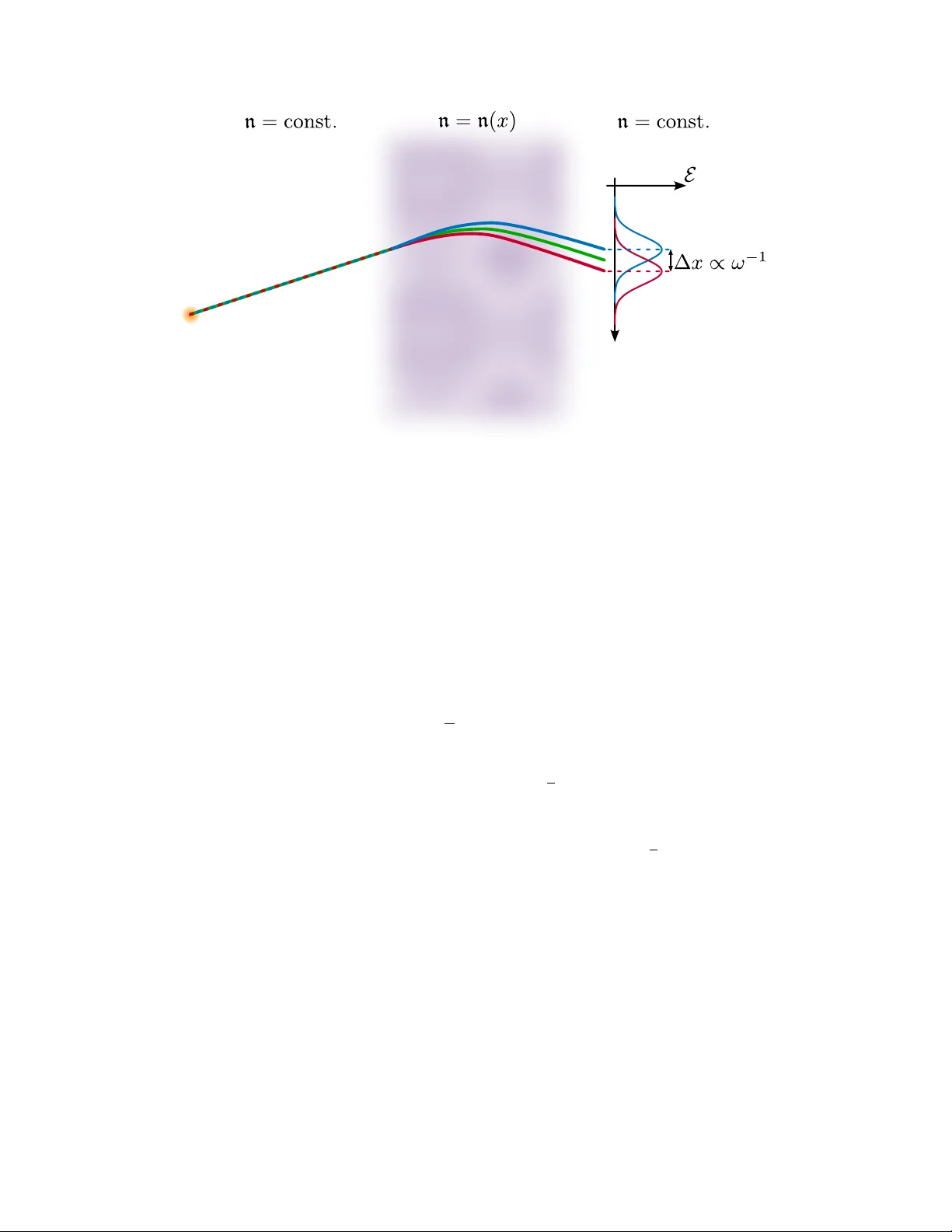
A mathematical description of the spin Hall eﬀect of ligh t in inhomogeneous media Sam C. Collingb ourne ∗ 1 , Marius A. Oancea † 2 , and Jan Sbierski ‡ 1 1 School of Mathematics and Maxwell Institute for Mathematical Sciences, University of Edinburgh, James Clerk Maxwell Building, Peter Guthrie T ait Road, Edinburgh, EH9 3FD, United Kingdom 2 Universit y of Vienna, F acult y of Physics, Boltzmanngasse 5, 1090 Vienna, Austria Abstract W e study Gaussian w av e pack et solutions for Maxwell’s equations in an isotropic, inhomogeneous medium and derive a system of ordinary diﬀeren tial equations that captures the leading-order correction to geo desic motion. The dynamical quan tities in this system are the energy centroid, the linear and angular momen tum, and the quadrup ole momen t. F urthermore, the system is closed to ﬁrst order in the inv erse frequency . As an immediate consequence, the energy cen troids of Gaussian wa v e pac kets with opp osite circular p olarisations generally propagate in diﬀerent directions, thereby providing a mathematical pro of of the spin Hall eﬀect of light in an inhomogeneous medium. Con ten ts 1 In tro duction 2 1.1 Discussion of main results . . . . . . . . . . . . . . . . . . . . . . . . . . . . . . . . . . . . . . 4 1.2 Ov erview of the pro of . . . . . . . . . . . . . . . . . . . . . . . . . . . . . . . . . . . . . . . . 5 1.3 Outline of the pap er . . . . . . . . . . . . . . . . . . . . . . . . . . . . . . . . . . . . . . . . . 6 2 Preliminaries 7 2.1 Notation and con ven tions . . . . . . . . . . . . . . . . . . . . . . . . . . . . . . . . . . . . . . 7 2.2 Maxw ell’s equations in an inhomogeneous medium . . . . . . . . . . . . . . . . . . . . . . . . 8 2.3 Energy , momen tum, and multipole moments . . . . . . . . . . . . . . . . . . . . . . . . . . . . 8 2.4 Optical geometry . . . . . . . . . . . . . . . . . . . . . . . . . . . . . . . . . . . . . . . . . . . 10 3 Main results 10 4 The approximate solutions 16 4.1 Construction of the Gaussian b eam appro ximation . . . . . . . . . . . . . . . . . . . . . . . . 19 4.1.1 Construction of the phase function . . . . . . . . . . . . . . . . . . . . . . . . . . . . . 24 4.1.2 Construction theorem . . . . . . . . . . . . . . . . . . . . . . . . . . . . . . . . . . . . 27 4.2 Conserv ation laws . . . . . . . . . . . . . . . . . . . . . . . . . . . . . . . . . . . . . . . . . . 29 4.3 The stationary phase appro ximation for the approximate solutions . . . . . . . . . . . . . . . 30 5 Construction of a one-parameter family of initial data 33 6 The energy estimate 36 ∗ sc.collingbourne@ed.ac.uk † marius.oancea@univie.ac.at ‡ jan.sbierski@ed.ac.uk 1 7 Appro ximation of exact solutions and pro of of main results 37 7.1 Pro of of Theorem 3.10 . . . . . . . . . . . . . . . . . . . . . . . . . . . . . . . . . . . . . . . . 40 A The stationary phase appro ximation 46 B Additional results and useful relations 47 C Deriv ation of the Gaussian beam equations 51 D Auxiliary computations 53 D.1 Computation of initial a verage quan tities and multipole moments . . . . . . . . . . . . . . . . 53 D.2 Computation for circularly p olarised initial data . . . . . . . . . . . . . . . . . . . . . . . . . 55 1 In tro duction Spin Hall eﬀects are present in man y areas of ph ysics, suc h as condensed matter ph ysics [ 1 – 8 ], optics [ 9 – 19 ], general relativity [ 20 – 36 ], and high energy physics [ 37 – 39 ]. The characteristic prop ert y of these eﬀects is that lo calised w av e pac kets carrying spin angular momen tum are scattered or propagated in a spin-dep endent w ay . This behaviour is due to spin-orbit coupling mec hanisms [ 1 , 9 ] represen ted b y mutual interactions b etw een the external (av erage position and a verage momentum) and the in ternal (spin angular momentum) degrees of freedom of a wa v e pack et. While on a fundamental lev el the description of such w av e pack ets is giv en by a partial diﬀerential equation (suc h as Schr¨ odinger, Dirac, Maxwell, linearised gra vity), spin Hall eﬀects are usually derived using semiclassical methods. This leads to an appro ximate description in terms of a system of ordinary diﬀeren tial equations, where the propagation of the w a ve pac k et is appro ximately represented as a p oin t particle that follows a spin-dependent tra jectory . In optics, the spin Hall eﬀect of l ight t ypically arises during the propagation of electromagnetic w av e pac k- ets in inhomogeneous media with a smo othly v arying refractiv e index [ 11 – 14 , 40 – 42 ], or in asso ciation with reﬂection and refraction pro cesses at the in terface betw een tw o distinct media where there is a discon tin uous jump of the refractive index [ 43 – 48 ] (similar eﬀects are also present for light propagating in optical ﬁbres [ 19 , 49 , 50 ]). Most importantly , spin Hall eﬀects of ligh t ha ve b een observed in man y exp erimen ts, where p olarisation-dep enden t shifts of the energy cen troids of electromagnetic wa ve pack ets ha ve b een measured [ 16 , 17 , 51 – 53 ]. An o verview of these eﬀects and their applications can be found in [ 9 , 10 ]. A sketc h of the spin Hall eﬀect of ligh t in an inhomogeneous medium is presen ted in Figure 1 (see also [ 9 ] for other similar illustrations of the eﬀect). Here, w e consider a medium with a smoothly v arying refractiv e index, where a central region is sandwiched b etw een tw o regions of constant refractiv e index. In particular, w e assume that there are no sharp interfaces and that the refractive index v aries smo othly b et ween these regions. In the region of constant refractive index to the left of the ﬁgure, w e prescrib e initial data representing lo calised wa ve pack ets, where the only diﬀerence betw een the considered w a ve pack ets is the state of circular p olarisation. F or reference, w e include the geometric optics geodesic ray represented in green, whic h is indep enden t of the state of p olarisation and the frequency . Ho wev er, if we include higher-order spin Hall corrections to the geometric optics approximation, the propagation of the wa ve pac kets b ecomes frequency- and p olarisation-dep endent. In this case, the rays follo wed by the centre of energy of the wa ve pac kets of opp osite circular p olarisation (blue and red ra ys in Figure 1 ) coincide with the geometric optics ra y (green ra y in Figure 1 ) in the initial region of constan t refractiv e index but drift apart in a frequency- and polarisation- dep enden t wa y as soon as the inhomogeneous region is reached. This p olarisation-dep endent propagation of electromagnetic wa ve pac kets represents the spin Hall eﬀect of ligh t. In comparison to the geometric optics ra y , the spin Hall ra ys will generally drift in a direction orthogonal to the direction of propagation and to the gradien t of the refractive index, and the magnitude of the drift is proportional to the wa velength. The 2 Figure 1: A sk etch of the spin Hall eﬀect of ligh t in an inhomogeneous medium. The geometric optics geodesic is represen ted by the green ra y , whic h is indep endent of the frequency and of the polarisation. When higher- order spin Hall corrections to the geometric optics approximation are included, we obtain frequency- and p olarisation-dep enden t ra ys. This leads to the spin Hall eﬀect of light, where the propagation of the energy cen troids of w av e pack ets with opp osite circular p olarisation is then represented by the blue and red ra ys. On the righ t part of the ﬁgure, the spin Hall ra y separation is also represented in terms of the shifted energy densities of the t wo w av e pack ets with opposite circular p olarisations. geometric optics rays are recov ered in the limit of zero w a velength, or equiv alen tly , inﬁnitely high frequency . In other w ords, the spin Hall correction term for geometric optics geo desics is prop ortional to [ 9 ] s ω p × ∇ n , (1.1) where s = ± 1 is a constant determined by the state of circular polarisation, ω is the frequency of the wa v e, p is the linear momen tum which represen ts (to leading order in 1 ω ) the direction of propagation of the wa ve pac ket and n is the refractive index of the medium. One ma y call the correction ( 1.1 ) to geo desic motion due to diﬀeren t circular p olarisations the ‘classical’ spin Hall eﬀect. Already here it is w orthwhile to p oint out that further correction terms to geo desic motion whic h are proportional to 1 ω are in general present (see Section 1.1 ). The deriv ations of the (classical) spin Hall eﬀect of light present in the physics literature generally start b y considering Maxwell’s equations and then applying certain approximations or high-frequency asymptotic expansions. A common route is represen ted by extensions of geometric optics and WKB-type expansions [ 41 , 42 ], sometimes com bined with paraxial approximations [ 11 , 13 ]. In this case, a geometric optics ansatz of the form ψ e i ω S , where S is a real phase function and ψ is a vector-v alued amplitude, is inserted into Maxw ell’s equations and the resulting equations at each order in ω are individually set to zero. This recov ers the well-kno wn geometric optics results represented by a Hamilton-Jacobi equation for S at the leading order in ω and a transp ort equation for the amplitude ψ at the next-to-leading order in ω . The Hamilton-Jacobi equation can be solved by the metho d of characteristics, leading to the geo desic rays of geometric optics. The transp ort equation determines the evolution of the shap e of the wa ve pac ket, as well as the evolution of the p olarisation, along the geometric optics rays. In particular, it is conv enient to express the part of the 3 transp ort equation for the polarisation in terms of a Berry connection, whic h can b e in tegrated to represent the evolution of the p olarisation in terms of a Berry phase (see [ 54 , 55 ] for a geometric deﬁnition of transp ort equations in terms of Berry connections). Within this framework, the spin Hall equations can be obtained by noting that the total phase of the ansatz ψ e i ω S is not only given b y the eikonal phase S , but that there is also a sub-leading Berry phase con tribution S B that comes from the complex v ector amplitude ψ . Thus, the total phase function is S + ω − 1 S B , and a modiﬁed Hamilton-Jacobi equation for it can be deriv ed b y com bining the Hamilton-Jacobi equation for S and the transport equation for ψ . The spin Hall equations represen ted b y the leading-order geo desic rays of geometric optics together with the spin-dep endent correction term in Eq. ( 1.1 ), are then obtained by applying the metho d of characteristics to the modiﬁed Hamilton-Jacobi equation. W e emphasise here that this approach only focuses on the sub-leading correction originating from the dynamics of the p olarisation, through the Berry phase and the Berry connection. In particular, there are no con tributions related to the shap e of the w av e pac k et (e.g., general angular momentum or quadrupole momen ts). F urthermore, we note that the correction to the geometrical optics rays is captured at the lev el of ‘corrected characteristics’ instead of the lev el of the tra jectory of the energy centroid. Those aspects will b e imp ortan t for comparison with the results that we presen t in the following. Diﬀeren t deriv ations of the spin Hall equations, based on other metho ds, hav e also been given. F or example, in Refs. [ 12 , 56 ] the authors used semiclassical metho ds (adapted from quantum mechanics and condensed matter physics [ 57 – 59 ]) to describ e the dynamics of wa v e pac kets with Berry curv ature corrections. Here also, similar to the previously discussed approac h, the main geometric ob jects describing the eﬀect are the Berry connection and the asso ciated Berry curv ature. Another deriv ation has also b een giv en in [ 14 , 15 ], where instead of starting from Maxwell’s equations the authors introduce a geometrically motiv ated form ulation of photons as classical particles. On a more mathematical level, a spin Hall eﬀect of light has been describ ed in [ 18 ], where the authors considered electromagnetic w av e pac kets in photonic crystals (optical materials with p erio dic structure). This result uses semiclassical metho ds based on the theory of pseudo diﬀeren tial op erators [ 60 – 62 ] to prov e Egorov-t yp e theorems for the dynamics of certain observ ables. 1.1 Discussion of main results In this pap er, w e present a precise mathematical theory of the propagation of Gaussian b eam 1 solutions to Maxwell’s equations in an inhomogeneous medium with refractiv e index n . This theory is based on the Gaussian b eam approximation 2 for hyperb olic partial diﬀerential equations, as, for example, presented in [ 67 , 68 ]: proﬁle functions for the Gaussian beam can be freely chosen as part of the initial data, which then determines a one-parameter family of Gaussian beam solutions, where the parameter is the frequency ω of the beam. As the frequency ω go es to inﬁnity , the spatial width of the Gaussian en velope of the b eam scales to zero lik e ω − 1 2 . W e show that for any given time T > 0, the follo wing ODE system is satisﬁed by this 1 W e emphasise here a diﬀerence in terminology compared to the optics literature. In our work, a Gaussian b eam represents a wa ve pac ket of ﬁnite energy that, at eac h time t , is localised in space in the sense that it decays exponentially in all three spatial directions a wa y from a reference point. On the other hand, in the optics literature the term Gaussian b eam is generally used to describe exact or approximate solutions of a wa ve equation or a paraxial equation that are exp onentially localised only in tw o spatial direction transverse to the spatial direction of propagation and which hav e inﬁnite energy [ 63 – 65 ]. 2 In the literature, this is also known as the complex WKB approximation [ 66 ]. 4 one-parameter family of Gaussian b eam solutions for times 0 ≤ t ≤ T (see Theorem 3.10 ): ˙ X i = 1 E n 2 P i − 1 E n 2 ϵ ij k J j ∇ k ln n − 1 E ˙ Q ij ∇ j ln n − 1 E 2 n 2 h P i Q j k ∇ j ∇ k ln n + 2 P j Q ik ( ∇ j ln n )( ∇ k ln n ) i + O ( ω − 2 ) , (1.2a) ˙ P i = E ∇ i ln n + Q j k ∇ i ∇ j ∇ k ln n + O ( ω − 2 ) , (1.2b) ˙ J i = ϵ ij k  P j ˙ X k + Q j l ∇ l ∇ k ln n  + O ( ω − 2 ) , (1.2c) ˙ Q ij = i ω − 1 E d dt ( A − 1 ) ij + O ( ω − 2 ) . (1.2d) Here, the constants implicit in the O -notation depend in particular on the c hosen proﬁle functions and the time of appro ximation T . In principle, these constan ts can be computed explicitly . F urthermore, E denotes the total energy (whic h is conserv ed in time), X the cen tre of energy , P the Mink owski linear momentum, J the Mink owski angular momen tum, and Q the quadrupole moment. Both the angular momen tum and the quadrup ole momen t are deﬁned with resp ect to the energy cen troid X . The deﬁnitions are given in Section 2.3 . F urthermore, in the abov e system, n and its deriv atives are all ev aluated at X ( t ) and A ( t ) denotes an inv ertible matrix whic h is purely imaginary and is uniquely determined for all time b y the c hosen proﬁle functions. In particular, this closes the ODE system, mo dulo the error terms O ( ω − 2 ). If one normalises the energy so that it is of order 1 (with resp ect to ω → ∞ ), then one can show that P is also of order 1 (see Remark 3.20 ) and J and Q are of order ω − 1 (see Proposition 3.15 ). As a consequence, the error terms are indeed negligible for large ω and the ODE system determines the ev olution of X , P , J , Q up to and including order ω − 1 . A t leading order ∼ 1, the solution ( X ( t ) , P ( t )) of the ab ov e ODE system is determined b y geo desic motion with respect to the optical metric, as discussed in Remark 3.20 . This recov ers the propagation of the energy cen troid according to the la ws of geometric optics in the limit ω → ∞ , and is represen ted by the green ray in Figure 1 . In addition to the precise mathematical theory , our approac h directly giv es a system inv olving the energy cen troid as a v ariable (which is accessible to exp erimen ts [ 16 , 17 , 52 ]) and, moreo ver, the system captures al l ω − 1 corrections to null geodesic motion: not just the in ternal spin angular momen tum, but indeed the total angular momen tum and also the quadrup ole momen t. The displacemen t ( 1.1 ) of the ‘classical’ spin Hall eﬀect arises from the second term on the right-hand side of ( 1.2a ) if one makes the idealised assumption that the wa v e only carries internal spin angular momentum (whic h is proportional to P ). This is presented in Prop osition 3.15 and Deﬁnition 3.25 with Eq. ( 3.27 ). T o the best of our kno wledge, this w ork represen ts the ﬁrst mathematical theory of the spin Hall eﬀect of ligh t in an inhomogeneous medium whic h is based on the Gaussian beam approximation. Ho wev er, for the Sc hr¨ odinger equation the Gaussian beam approximation has already been used to capture subleading eﬀects on the propagation depending on the shap e of the w av e pac ket [ 69 ] as well as the anomalous Hall eﬀect in inhomogeneous perio dic media [ 70 ], which has structural similarities to the spin Hall eﬀect of ligh t. Note that in [ 70 ] an eﬀectiv e particle- ﬁeld system is derived, while our ODE system ( 1.2 ) corresponds to an eﬀective particle system. 1.2 Ov erview of the pro of W e work at the level of the electric ﬁeld E and the magnetising ﬁeld H and construct appro ximate Gaussian b eam solutions of the form ˆ E = ω 3 / 4 Re  ( e 0 + ω − 1 e 1 + ω − 2 e 2 ) e i ω ϕ  , ˆ H = ω 3 / 4 Re  ( h 0 + ω − 1 h 1 + ω − 2 h 2 ) e i ω ϕ  . (1.3) 5 Here, e j , h j , and ϕ are the proﬁle functions of the b eam. In con trast to unconstrained h yp erb olic PDEs (see, for example, [ 67 , 68 ]), one cannot just take the induced initial data of the appro ximate solution as initial data for Maxw ell’s equations, since in general it does not satisfy the constrain t equations. Here, we use Bogo vskii’s op erator [ 71 , 72 ] to solv e for a compactly supp orted error term, whic h we add to the approximate initial data to obtain exact Gaussian b eam initial data for Maxwell’s equations. Our main theorem is phrased in terms of suc h compactly supp orted exact Gaussian b eam initial data. Using energy estimates, we get quan titative upp er b ounds on the diﬀerence b etw een exact and appro xi- mate solutions in a ﬁnite time range. This gives us on the one hand the a priori estimate | X ( t ) − γ ( t ) | R 3 = O ( ω − 1 ) , (1.4) where γ is the geodesic determined b y the optical geometry and γ ( t ) is the point of stationary phase for the energy and momen tum densit y of the approximate solution at time t . On the other hand, w e obtain that the energy centroid ˆ X of the approximate solution is O ( ω − 2 )-close to X – and similarly for the linear and angular momen tum and the quadrup ole moment. In principle ˆ X ( t ) can b e computed to order ω − 1 directly from the proﬁle functions of the appro ximate solution (see Prop osition 4.105 ), which ma y b e of use for n umerical ev aluation in concrete situations. Ho wev er, theoretically it hides the explicit dynamical dep endence of the energy cen troid on the ﬁrst few m ultip ole momen ts. T o derive the closed ODE system ( 1.2 ) for these momen ts, w e pro ceed as follows: Maxwell’s equations giv e us ˙ X i = 1 E Z R 3 n − 2 S i d 3 x, (1.5) where S is the momen tum density and P i ( t ) := R R 3 S i ( t, x ) d 3 x . W e no w T a ylor-expand n − 2 ( x ) around X ( t ). The ﬁrst (constant) term can b e pulled out of the integral so that w e end up with 1 E n − 2 | X ( t ) P i ( t ), whic h is the ﬁrst term on the right-hand side of ( 1.2a ). The remaining terms in the T a ylor expansion yield higher m ultip ole momen ts. The antisymmetric ﬁrst momen t of S gives us the angular momen tum term in Eq. ( 1.2a ), while the symmetric ﬁrst moment can b e related to the time deriv ativ e of the quadrupole moment. T o treat the second momen ts, w e ﬁrst use the fact that they are O ( ω − 2 )-close to those of the approximate solution. W e then use the structure of the appro ximate solution together with a stationary phase expansion and Eq. ( 1.4 ) to write them, to leading order, in terms of linear momentum and quadrupole moment. The third moments can b e sho wn to b e negligible – again using a stationary phase expansion for the approximate solution. The ev olution equations for P , J , and Q can b e dealt with in a similar w a y . Finally , the determination of the correct order in ω of the diﬀeren t moments again follo ws from the stationary phase expansion. 1.3 Outline of the pap er W e start with some preliminaries in Section 2 : in Section 2.1 w e lay out con ven tions used throughout this pap er, in Section 2.2 we recall Maxw ell’s equations in an inhomogeneous medium and deﬁne the notions of total energy , linear momen tum, angular momentum, dip ole momen t, and quadrup ole moment. The ev olution equations of those quantities are also collated here. In Section 2.4 the optical geometry is deﬁned and the equations of ray optics (geo desics) recalled. Our main results are stated and discussed in detail in Section 3 . The pro of of our main results is spread across Sections 4 to 7 : in Section 4 the construction of approximate Gaussian beam solutions is carried out, and in Section 5 exact Maxw ell initial data satisfying the constraint equations is constructed from the induced initial data of the approximate solution b y adding a suitable small p erturbation. The fundamental energy estimate for Maxwell’s equations is recalled in Section 6 , which is used to control the error betw een the exact and appro ximate Gaussian b eam solution. The deriv ation of our ODE system is then concluded in Section 7 . F our appendices are pro vided: App endix A recalls the stationary 6 phase approximation for the conv enience of the reader, while App endices B to D provide more details on and auxiliary computations for the Gaussian b eam appro ximation for Maxwell’s equations. Ac kno wledgemen ts Sam C. Collingbourne and Jan Sbierski ackno wledge support through the Roy al Society Universit y Researc h F ello wship URF \ R1 \ 211216. This research was funded in whole or in part b y the Austrian Science F und (FWF) 10.55776/PIN9589124 . Jan Sbierski also thanks Sung-Jin Oh for discussions ab out Bogo vskii’s op er- ator. 2 Preliminaries In this section, we review our notation and introduce the basic deﬁnitions to b e used in the rest of the pap er. The starting p oin t for the formulation of our results is represented by Maxwell’s equations in an inhomogeneous medium, together with the asso ciated observ able quan tities, such as total energy and cen tre of energy , linear and angular momen tum, and quadrup ole moment. W e also review the optical geometry asso ciated with Gordon’s optical metric, whic h serves as a geodesic formulation of ra y optics. 2.1 Notation and conv entions • W e w ork in Mink owski spacetime R 1+3 using global Cartesian coordinates ( t, x ), where the spatial co ordinates are denoted as x = x i = ( x 1 , x 2 , x 3 ). • W e use lo wercase Latin indices that range from 1 to 3 to denote coordinate components x i , as w ell as v ector comp onents v i . The summation conv en tion v i w i = P 3 i =1 v i w i is used for rep eated indices. T o a void p ossible confusion b etw een indices and the imaginary unit, we use the notation i 2 = − 1. W e also ﬁx the complex square ro ot b y imp osing a branch cut along the negativ e real axis. • W e denote spatial partial deriv atives by ∇ i and spacetime partial deriv atives by ∂ ν . Indices ν, κ, . . . denote spacetime indices running from 0 to 3. • The electric p ermittivity ε : R 3 → R and the magnetic p ermeabilit y µ : R 3 → R are p ositive smo oth real scalar functions on R 3 with 0 < c m ≤ ε ≤ C m and 0 < c m ≤ µ ≤ C m for some positive constants c m , C m . The refractive index of the inhomogeneous medium is deﬁned as n = √ εµ , and we assume that n ≥ 1. • F or v ∈ R 3 , deﬁne ( ⋆v ) ij = ϵ ij k v k , where ϵ ij k is the Levi-Civita sym b ol. • Given a spacetime vector or v ector ﬁeld v , then v denotes the purely spatial part with respect to the standard basis. • Our con ven tion for raising and low ering spatial indices is with resp ect to the Euclidean metric δ . If a raising or lo w ering of an index is accompanied by ♯ or ♭ , then the raising or low ering is with resp ect to g = n 2 δ . • Similarly , the norm | X | := √ X i X i of a v ector in R 3 is alwa ys with respect to the Euclidean metric. F or a complex v ector X ∈ C 3 the norm is deﬁned b y | X | := p X i X i . The dot product for real as well as for complex vectors X , Y is deﬁned by X · Y = X i Y i . Note that for a complex vector X we ha ve | X | 2 = X · X and X · X is not necessarily real. 7 • W e denote the closure of a set K by cl( K ). • Given a quantit y Q , which in particular depends on ω > 1, we employ the notation Q = O ( ω − p ) if there exists a p ositiv e constant C , whose dep endence will b e made explicit, such that |Q| ≤ C ω − p . • Given a function Q : R 3 → C , whic h furthermore dep ends on ω > 1, we employ the notation Q ( x ) = O L q ( R 3 ) ( ω − p ) if there exists a positive constan t C , whose dependence will b e made explicit, such that ∥Q∥ L q ( R 3 ) ≤ C ω − p . • Let f : R 1+3 → C or f : R → C be a smo oth function. W e use the notation ˙ f = ∂ t f and ¨ f = ∂ 2 t f . • Let α = ( α 1 , α 2 , α 3 ) ∈ N 3 and D α b e deﬁned b y D α := ( ∇ x 1 ) α 1 ( ∇ x 2 ) α 2 ( ∇ x 3 ) α 3 . 2.2 Maxw ell’s equations in an inhomogeneous medium This section recalls the basic theory of Maxwell’s equations in an inhomogeneous medium, which is at rest in Mink owski spacetime with resp ect to the timelik e Killing vector ﬁeld ∂ t . In a general medium, the equations can b e written as [ 73 ] ∇ · D = 4 π ρ, (2.1a) ∇ · B = 0 , (2.1b) ∇ × E + 1 c ˙ B = 0 , (2.1c) ∇ × H − 1 c ˙ D = 4 π c j, (2.1d) where E is the electric ﬁeld, D the displacement ﬁeld, B the magnetic ﬁeld, and H the magnetising ﬁeld. All these ﬁelds are smooth functions from (subsets of ) R 1+3 to R 3 . W e work in units where the sp eed of ligh t is c = 1, and w e restrict our atten tion to the ca se where there are no c harges or currents ( ρ = 0 and j = 0). F urthermore, we consider inhomogeneous media described by the constitutiv e relations D = εE , B = µH, (2.2) where ε = ε ( x ) and µ = µ ( x ) are positive smo oth real scalar functions on R 3 with 0 < c m ≤ ε ≤ C m and 0 < c m ≤ µ ≤ C m for some positive constants c m , C m . The refractiv e index is then deﬁned as n = √ εµ , and to simplify the presen tation, w e also assume the ph ysically realistic assumption that n ≥ 1. In this case, Maxw ell’s equations can b e written as ∇ · E + E · ∇ ln ε = 0 , (2.3a) ∇ · H + H · ∇ ln µ = 0 , (2.3b) ∇ × E + µ ˙ H = 0 , (2.3c) ∇ × H − ε ˙ E = 0 . (2.3d) All solutions to ( 2.3 ) considered in this pap er will hav e compact spatial support. 2.3 Energy , momen tum, and multipole momen ts The energy densit y of the electromagnetic ﬁeld is deﬁned as E := 1 2 ( E · D + H · B ) = 1 2 ( εE · E + µH · H ) , (2.4) 8 and the momen tum density (Mink owski’s P oyn ting vector) is deﬁned as S := D × B = n 2 E × H . (2.5) Using Maxw ell’s equations ( 2.3 ), the energy densit y and momen tum densit y are related through the con tinuit y equation ˙ E + ∇ ·  n − 2 S  = 0 . (2.6) The total energy of the electromagnetic ﬁeld is deﬁned as E ( t ) := Z R 3 E ( t, x ) d 3 x. (2.7) If we assume that the electromagnetic ﬁeld v anishes suﬃciently fast at inﬁnit y – for example, if the ﬁeld is of compact spatial supp ort, as is the case in this pap er – it follo ws from the contin uity equation that the total energy is conserv ed: ˙ E = 0 . (2.8) W e deﬁne the energy centroid (or also cen tre of energy) of the electromagnetic ﬁeld as X i ( t ) := 1 E Z R 3 x i E ( t, x ) d 3 x. (2.9) T aking the time deriv ative of the abov e equation and using Maxwell’s equations ( 2.3 ) in combination with suﬃcien tly fast decay to wards inﬁnit y , we obtain ˙ X i = 1 E Z R 3 n − 2 S i d 3 x. (2.10) The total linear momen tum is deﬁned as P i ( t ) := Z R 3 S i ( t, x ) d 3 x. (2.11) T aking the time deriv ativ e and using Maxw ell’s equations ( 2.3 ) in combination with suﬃcien tly fast deca y to wards inﬁnit y we obtain ˙ P i = 1 2 Z R 3 ( εE · E ∇ i ln ε + µH · H ∇ i ln µ ) d 3 x. (2.12) The total angular momen tum with resp ect to the energy centroid X ( t ) is deﬁned as J i ( t ) := Z R 3 ϵ ij k r j ( t, x ) S k ( t, x ) d 3 x, (2.13) where r j ( t, x ) := x j − X j ( t ). T aking the time deriv ative, w e obtain ˙ J i = ϵ ij k P j ˙ X k + Z R 3 ϵ ij k r j ˙ S k d 3 x = ϵ ij k P j ˙ X k + 1 2 Z R 3 ϵ ij k r j  εE · E ∇ k ln ε + µH · H ∇ k ln µ  d 3 x. (2.14) The dip ole and quadrup ole moments of the energy density with resp ect to the energy centroid X ( t ) are deﬁned as D i ( t ) := Z R 3 r i ( t, x ) E ( t, x ) d 3 x, (2.15a) Q ij ( t ) := Z R 3 r i ( t, x ) r j ( t, x ) E ( t, x ) d 3 x. (2.15b) 9 It follo ws from the deﬁnition ( 2.9 ) of the energy centroid that D i = Z R 3 x i E d 3 x − X i Z R 3 E d 3 x = 0 . (2.16) Using Maxwell’s equations ( 2.3 ) and again suﬃcien tly fast decay at inﬁnit y , the time deriv ative of the quadrup ole momen t is ˙ Q ij = 2 Z R 3 n − 2 r ( i S j ) d 3 x. (2.17) 2.4 Optical geometry Recall that the optical metric on R × R 3 = R 1+3 as deﬁned b y Gordon [ 74 ] is giv en b y − n − 2 dt 2 + δ , where δ = dx 1 ⊗ dx 1 + dx 2 ⊗ dx 2 + dx 3 ⊗ dx 3 is the Euclidean metric on R 3 . In this pap er, it will b e useful to w ork with the conformally rescaled optical metric g := − dt 2 + n 2 δ =: − dt ⊗ dt + g (2.18) on R 1+3 , where w e hav e deﬁned the Riemannian metric g := n 2 δ on R 3 . Note that g is a Loren tzian metric. W e denote the Christoﬀel symbols with resp ect to g by Γ and those with resp ect to g b y Γ. A straight- forw ard inv estigation then giv es Γ i j k = Γ i j k for i, j, k ∈ { 1 , 2 , 3 } and all other Christoﬀel symbols of g with at least one time-comp onen t v anish. Thus, the geodesic equation on ( R 1+3 , g ) takes the form ¨ γ t = 0 , (2.19a) ¨ γ i = − Γ i j k ˙ γ j ˙ γ k . (2.19b) Th us, it follo ws that t 7→ γ ( t ) =  t, γ ( t )  is a g -n ull geodesic, if and only if, t 7→ γ ( t ) is a geo desic in ( R 3 , g ) parametrised b y g -arclength. W e no w fo cus on the spatial geometry of ( R 3 , g ). Consider the Hamiltonian H ( x, p ) := 1 2 g − 1 | x ( p, p ) on phase space T ∗ R 3 ≃ R 6 . Then the Hamiltonian equations ˙ x i = ∂ H ∂ p i = g ij p j , (2.20a) ˙ p i = − ∂ H ∂ x i = 2 H∇ i ln n , (2.20b) generate the geodesic ﬂow on phase space. Consider now a geodesic γ on ( R 3 , g ) which is parametrised by g -arclength. If we set p i := ˙ γ ♭ i := g ij ˙ γ j , w e then hav e H ( γ , ˙ γ ♭ ) ≡ 1 2 and th us the equations ˙ γ i = g ij p j = 1 n 2 δ ij p j , (2.21a) ˙ p i = ∇ i ln n (2.21b) are satisﬁed. 3 Main results There are v arious lo calised high-frequency solutions of Maxw ell’s equations whose energy centroids propagate, to leading order in one ov er frequency , according to n ull geo desic motion. In this pap er, w e restrict ourselves to a sp ecial class of suc h localised high-frequency solutions, namely those arising from Gaussian b eam initial data (deﬁned below). F or suc h solutions, we describ e the sub-leading correction to the equation of motion of the energy cen troid. W e b egin by deﬁning the class of initial data that w e consider in this pap er. 10 Deﬁnition 3.1. K -supp orte d Gaussian b e am initial data of or der 2 for Maxwel l’s e quations ( 2.3 ) is a one- p ar ameter family  E ( · ; ω ) , H ( · ; ω )  ∈ C ∞ 0 ( K , R 3 ) × C ∞ 0 ( K , R 3 ) with ω > 1 of the form E ( x ; ω ) = ω 3 / 4 Re n  e 0 ( x ) + ω − 1 e 1 ( x )  e i ω ϕ ( x ) o + O L 2 ( R 3 ) ( ω − 2 ) , (3.2a) H ( x ; ω ) = ω 3 / 4 Re n  h 0 ( x ) + ω − 1 h 1 ( x )  e i ω ϕ ( x ) o + O L 2 ( R 3 ) ( ω − 2 ) , (3.2b) such that for x 0 ∈ R 3 and a pr e-c omp act op en neighb ourho o d K ⊆ R 3 of x 0 we have 1. ϕ ∈ C ∞ ( R 3 , C ) with Im ϕ ≥ 0 and Im ϕ | x 0 = 0 , ∇ Im ϕ | x 0 = 0 , ∇ Re ϕ | x 0  = 0 , Im ∇ i ∇ j ϕ | x 0 is a p ositive deﬁnite matrix 3 , and ∇ Im ϕ  = 0 in cl( K ) \ { x 0 } . 2. e A , h A ∈ C ∞ 0 ( K , C 3 ) for A ∈ { 0 , 1 } with e 0 | x 0  = 0 and D α  e k 0 ∇ k ϕ     x 0 = 0 ∀| α | ≤ 5 , (3.3a) D α  e k 1 ∇ k ϕ − idiv e 0 − i e k 0 ∇ k ln ε     x 0 = 0 ∀| α | ≤ 3 . (3.3b) Mor e over, the ﬁrst terms in the T aylor exp ansion of h A ar ound x 0 ar e r elate d to those of e A and ϕ by D α h i 0     x 0 = D α  − 1 µ ˙ ϕ ϵ ij k e k 0 ∇ j ϕ      x 0 ∀| α | ≤ 5 , (3.4a) D α h i 1     x 0 = D α  − 1 µ ˙ ϕ ϵ ij k e k 1 ∇ j ϕ + i µ ˙ ϕ ϵ ij k ∇ j e k 0 + i n 2 ˙ ϕ 2 ∇ j ϕ ∇ j h i 0 + i 2 n 2 ˙ ϕ 2  h i 0 ∆ ϕ − n 2 h i 0 ¨ ϕ + ∇ i ϕ h m 0 ∇ m ln n 2 − h i 0 ∇ m ϕ ∇ m ln ε       x 0 ∀| α | ≤ 3 , (3.4b) wher e ˙ ϕ and ¨ ϕ c an b e c ompute d naively at x 0 , up to or der 5 and 3 r esp e ctively, fr om the formulas 4 ˙ ϕ = − 1 n p ∇ i ϕ ∇ i ϕ , ¨ ϕ = ∇ j ϕ n p ∇ i ϕ ∇ i ϕ ∇ j p ∇ i ϕ ∇ i ϕ n ! . (3.5) 3. E ( · ; ω ) and H ( · ; ω ) satisfy the c onstr aint e quations ( 2.3a ) and ( 2.3b ) for e ach ω > 1 . A priori it migh t not b e ob vious that the class of K -supp orted Gaussian b eam initial data of order 2 is non- empt y . That it is indeed not just non-empt y , but a very ric h class of initial data is shown in Theorems 4.89 and 5.1 . The construction of approximate Gaussian b eam solutions to h yp erb olic PDEs is w ell kno wn and is given, for example, in [ 67 ], [ 68 ]. Here, we carry out this construction in Theorem 4.89 for Maxw ell’s equations ( 2.3 ), whic h constitute a c onstr aine d h yperb olic system. As a consequence, it remains to show that one can p erturb the compactly supp orted appro ximate initial data to obtain compactly supp orted data whic h identically satisﬁes the constrain t equations. This is done in Theorem 5.1 . Giv en suc h K -supp orted Gaussian b eam initial data of order 2 together with the p oint x 0 ∈ R 3 , there are the following asso ciated dynamical structures which naturally en ter in to the ODE system describ ed in the main Theorem 3.10 . These structures are determined purely by the optical geometry and the Gaussian b eam initial data. F or this we deﬁne the constan t c γ :=  1 n   ∇ ϕ |      x 0 = − ˙ ϕ | x 0 > 0 . (3.6) 3 Note that this implies that Im ∇ i ∇ j ϕ | x 0 is inv ertible. 4 Recall that √ denotes the complex square root (with a branch cut along the negative real axis). 11 Firstly , we consider the (real and n ull) spacetime v ector ∂ t + ∇ i ϕ n |∇ ϕ | ∂ i = ∂ t + 1 c γ ∇ i ϕ n 2 ∈ T (0 ,x 0 ) R 1+3 and the aﬃnely parametrised g -null geo desic γ generated by these initial data, which is of the form t γ 7→ ( t, γ ( t )). Recall from Section 2.4 that γ is a Riemannian geo desic in ( R 3 , g ) emanating from x 0 with tangen t ∇ i ϕ n |∇ ϕ | ∂ i that is parametrised b y g -arclength and satisﬁes Eq. ( 2.21 ). Secondly , we then consider the follo wing time-dep endent real 3 × 3-matrices along γ L ij ( t ) = − 1 n 2 c γ  n 2 ˙ γ i ˙ γ j − δ ij     γ ( t ) , (3.7a) N ij ( t ) = −  ∇ i ln n  ˙ γ j    γ ( t ) , (3.7b) R ij ( t ) = − c γ h ∇ i ∇ j ln n −  ∇ i ln n  ∇ j ln n  i    γ ( t ) (3.7c) and w e solve the follo wing matrix Riccati equation 5 d dt M + M · L · M + N · M + M · N T + R = 0 (3.8) with initial data M ij (0) := ∇ i ∇ j ϕ | x 0 . In the proof of Prop osition 4.55 it is sho wn that due to Im ∇ i ∇ j ϕ | x 0 b eing p ositiv e deﬁnite, this ODE has a unique smo oth solution t 7→ M ( t ) ∈ M at (3 × 3; C ) for all t ≥ 0 and A ij ( t ) := 2i · Im M ij ( t ) (3.9) is inv ertible for all t ≥ 0. The in verse of the matrix A is the dynamical structure that en ters into the ODE system b elo w. The follo wing is the main theorem of this pap er: Theorem 3.10. L et K -supp orte d Gaussian b e am initial data of or der 2 as in Deﬁnition 3.1 b e given and c onsider the c orr esp onding solution ( E , H ) to Maxwel l’s e quations ( 2.3 ) . Construct the nul l ge o desic γ and time-dep endent pur ely imaginary and invertible matrix A ij ( t ) as deﬁne d ab ove. L et T > 0 b e given. Then for al l 0 ≤ t ≤ T the fol lowing system of ODEs is satisﬁe d by the solution ( E , H ) : ˙ X i = 1 E n 2 P i − 1 E n 2 ϵ ij k J j ∇ k ln n − 1 E ˙ Q ij ∇ j ln n − 1 E 2 n 2 h P i Q j k ∇ j ∇ k ln n + 2 P j Q ik ( ∇ j ln n )( ∇ k ln n ) i + O ( ω − 2 ) , (3.11a) ˙ P i = E ∇ i ln n + Q j k ∇ i ∇ j ∇ k ln n + O ( ω − 2 ) , (3.11b) ˙ J i = ϵ ij k  P j ˙ X k + Q j l ∇ l ∇ k ln n  + O ( ω − 2 ) , (3.11c) ˙ Q ij = i ω − 1 E d dt ( A − 1 ) ij + O ( ω − 2 ) . (3.11d) Her e, n and its derivatives ar e al l evaluate d at X ( t ) . The c onstant implicit in the O -notation dep ends only on the c onstants implicit in the O L 2 ( R 3 ) -terms in Eq. ( 3.2 ) , the pr oﬁle functions ϕ , e A , and h A for A = 0 , 1 , the functions ε and µ , and the time of appr oximation T . Note that by deﬁnition ( 3.9 ), the matrix A is purely imaginary , so the ﬁrst term on the righ t-hand side of ( 3.11d ) is indeed real. W e emphasise that in this theorem, if T > 0 is ﬁxed, ω > 1 has to b e c hosen large enough for the error terms to b e small enough. Our pro of relies on the v alidity of the Gaussian b eam approximation. If the electric permittivity ε and magnetic p ermeabilit y µ are giv en, and if the proﬁle functions ϕ , e A , and h A for 5 Here, · stands for matrix multiplication and T for matrix transpose. 12 A = 0 , 1 of the initial data are known together with a b ound on the error terms in Eq. ( 3.2 ), then an explicit, T -dep endent b ound on the error terms in Eq. ( 3.11 ) is , in principle, computable from our pro of, and thus an estimate on ho w big ω has to b e chosen for a satisfactory appro ximation. T o complement Theorem 3.10 , the initial v alues of the a verage quan tities and m ultip ole momen ts can be computed directly from the Gaussian b eam initial data. Prop osition 3.12. Consider initial data as in Deﬁnition 3.1 . Then, the c orr esp onding ener gy E and initial data for the system of ODEs ( 3.11 ) ar e E = 1 q det  1 2 π i A   u + ω − 1 L 1 u     x 0 + O ( ω − 2 ) , (3.13a) X i (0) = x i 0 + i ω − 1 E q det  1 2 π i A  ( A − 1 ) ia h ∇ a u − i u ( A − 1 ) bc ∇ a ∇ b ∇ c Im ϕ i    x 0 + O ( ω − 2 ) , (3.13b) P i (0) = 1 q det  1 2 π i A   v i + ω − 1 L 1 v i     x 0 + O ( ω − 2 ) , (3.13c) J i (0) = ϵ ij k r j P k (0) + i ω − 1 q det  1 2 π i A  ϵ ij k ( A − 1 ) j a h ∇ a v k − i v k ( A − 1 ) bc ∇ a ∇ b ∇ c Im ϕ i    x 0 + O ( ω − 2 ) , (3.13d) Q ij (0) = i ω − 1 E ( A − 1 ) ij + O ( ω − 2 ) , (3.13e) wher e L 1 is the diﬀer ential op er ator deﬁne d in Eq. ( A.3 ) with f ( x ) = 2i Im ϕ , A ij = A ij (0) = 2i ∇ i ∇ j Im ϕ | x 0 , r j = x j 0 − X j (0) and u = 1 4  ε e 0 · e 0 + µ h 0 · h 0  + ω − 1 2 Re  ε e 0 · e 1 + µ h 0 · h 1  , (3.14a) v = n 2 2 Re  e 0 × h 0  + ω − 1 n 2 2 Re  e 0 × h 1 + e 1 × h 0  . (3.14b) Pr o of. The pro of can b e found in App endix D.1 . Prop osition 3.15. Given initial data as in Deﬁnition 3.1 , the total angular momentum and the quadrup ole moment for al l t ∈ [0 , T ] ar e J i ( t ) = ω − 1 E ˙ ϕ | x 0  s − i ϵ abc P a ( t ) | P ( t ) | ( A − 1 ) bd ( t ) B c d ( t )  P i ( t ) | P ( t ) | + i ω − 1 E ˙ ϕ | x 0 ϵ iab  P c ( t ) | P ( t ) | ( A − 1 ) cd ( t ) B a d ( t ) − ˙ ϕ | x 0 E | P ( t ) | ( A − 1 ) ac ∇ c ln n  P b ( t ) | P ( t ) | + O ( ω − 2 ) , (3.16a) Q ij ( t ) = i ω − 1 E ( A − 1 ) ij ( t ) + O ( ω − 2 ) , (3.16b) wher e B ij ( t ) = Re M ij ( t ) and the c onstant s ∈ [ − 1 , 1] is determine d by the state of p olarisation of the initial data (with s = ± 1 for cir cular p olarisation) as s = i n e 0 · h 0 ε e 0 · e 0     x 0 . (3.17) Pr o of. See Section 7 . Based on Eq. ( 3.16a ), w e note that there are several contributions to the total angular momentum carried b y the wa ve pac ket. The term prop ortional to s and aligned with the longitudinal direction of P is called spin angular momentum and is determined b y the state of p olarisation. In other w ords, this is an intrinsic 13 angular momen tum contribution related to the spin-1 nature of the electromagnetic ﬁeld. When combined with Eq. ( 3.11a ), the spin angular momentum giv es the spin Hall correction term ( 1.1 ) that is commonly discussed in the literature [ 9 ]. The other terms in Eq. ( 3.16a ) provide additional transverse and longitudinal angular momen tum contributions that directly dep end on the shap e and phase proﬁle of the w av e pac ket through the A and B matrices. W e emphasise that these additional terms are not related to an y v ortex-t yp e structures (such as in the case of Laguerre-Gauss beams) [ 75 , 76 ], but rather to the asymmetry or astigmatism that can b e present in the Gaussian proﬁle of the wa v e pack et [ 77 , 78 ]. In any case, all these additional terms pro vide contributions to the spin Hall eﬀect that ha ve not been previously discussed in the literature. Remark 3.18 (On the form of the ODE system ( 3.11 )) . 1. Equation ( 3.11a ) c an b e inserte d into the right- hand side of e quation ( 3.11c ) to obtain an ODE system in c anonic al form. 2. Equation ( 3.11d ) c an b e solve d dir e ctly to give ( 3.16b ) . This c an b e inserte d in the ﬁrst thr e e e quations to get a close d system for X , P , J alone to gether with the for cing term ( A − 1 ) ij ( t ) : ˙ X i ( t ) = 1 E n 2 P i ( t ) − 1 E n 2 ϵ ij k J j ( t ) ∇ k ln n − i ω − 1 d dt ( A − 1 ) ij ( t ) ∇ j ln n − i ω − 1 E n 2 h P i ( t )( A − 1 ) j k ( t ) ∇ j ∇ k ln n + 2 P j ( t )( A − 1 ) ik ( t )( ∇ j ln n )( ∇ k ln n ) i + O ( ω − 2 ) , (3.19a) ˙ P i ( t ) = E ∇ i ln n + i ω − 1 E ( A − 1 ) j k ( t ) ∇ i ∇ j ∇ k ln n + O ( ω − 2 ) , (3.19b) ˙ J i ( t ) = ϵ ij k h P j ( t ) ˙ X k ( t ) + i ω − 1 E ( A − 1 ) j l ( t ) ∇ l ∇ k ln n i + O ( ω − 2 ) . (3.19c) Remark 3.20 (Null geo desic motion at leading order) . We investigate the le ading or der b ehaviour of the solution to Eq. ( 3.19 ) . F or 0 ≤ t ≤ T we dir e ctly obtain fr om Eq. ( 3.19b ) that P i ( t ) = O (1) . (3.21) Inserting ( 3.19a ) into ( 3.19c ) and only ke eping le ading or der terms gives ˙ J i ( t ) = P m ( t ) J m ( t ) E n 2 ∇ i ln n − P m ( t ) ∇ m ln n E n 2 J i ( t ) + O ( ω − 1 ) . (3.22) Now, fr om Eqs. ( 3.21 ) and ( 3.13d ) it fol lows that J i ( t ) = O ( ω − 1 ) for 0 ≤ t ≤ T (or inde e d this fol lows fr om ( 3.16 ) ). Putting this information b ack into Eq. ( 3.19a ) , the le ading or der b ehaviour of the system ( 3.19 ) r e duc es to ˙ X i ( t ) = 1 E n 2 P i ( t ) + O ( ω − 1 ) , (3.23a) ˙ P i ( t ) = E ∇ i ln n + O ( ω − 1 ) . (3.23b) Now, with X i ( t ) = γ i ( t ) and P i ( t ) = E · p i ( t ) = E · ˙ γ ♭ i , (3.24) we se e that Eq. ( 3.23 ) is e quivalent to le ading or der to Eq. ( 2.21 ) – and by ( 3.13b ) , ( 3.13c ) the initial values agr e e. Henc e, due to the uniqueness of the initial value pr oblem, the solution  X ( t ) , P ( t )  is given by ( 3.24 ) to le ading or der. We have thus shown that, to le ading or der, Eq. ( 3.19c ) for the angular momentum dr ops out and the evolution of  X ( t ) , P ( t )  is determine d by nul l ge o desic motion. The c ontent of The or em 3.10 , or of Eq. ( 3.19 ) , is to give an ODE system which determines the c orr e ction to nul l ge o desic motion for the ener gy c entr oid to the ﬁrst suble ading or der in ω − 1 . This deviation fr om nul l ge o desic motion dep ends not only on the initial p osition and initial momentum, but also on the initial angular momentum and the initial quadrup ole moment. However, it c an stil l b e describ e d in terms of ordinary diﬀer ential e quations as a p article system! 14 Finally , we discuss how the ODE system ( 3.11 ) (or ( 3.19 )) can be used to describe the spin Hall eﬀect of ligh t in an inhomogeneous medium. F or this we consider a point x 0 ∈ R 3 that lies outside the inhomogeneous medium or at least in a region where the medium is nearly homogeneous in the sense that D α ε | x 0 = 0 = D α µ | x 0 for all 1 ≤ | α | ≤ 3. W e no w prepare left and righ t circularly p olarised Gaussian beam initial data in the vicinity of this point whic h, to leading order, is ‘iden tical up to p olarisation’. Mathematically , this is captured as follo ws: Deﬁnition 3.25 (A class of circularly polarised initial data) . Assume that the me dium is ne arly homo gene ous ne ar x 0 ∈ R 3 in the sense that D α ε | x 0 = 0 = D α µ | x 0 for al l 1 ≤ | α | ≤ 3 . Then K -supp orte d Gaussian b e am initial data of or der 2 as in Deﬁnition 3.1 is c al le d cir cularly p olarise d if, for  ∇ ϕ |∇ ϕ |    x 0 , X, Y  b eing a p ositively oriente d orthonormal fr ame at x 0 , wher e X and Y ar e r e al ve ctors, we have 1. e 0 | x 0 = a √ 2 ( X − i sY ) , wher e s = ± 1 and a is a strictly p ositive r e al c onstant. 2. Re ∇ a ∇ b ϕ | x 0 = 0 (or e quivalently ∇ a ∇ b ϕ | x 0 = 1 2 A ab ) and D α ϕ | x 0 = 0 for al l 3 ≤ | α | ≤ 4 . 3. ∇ a e i 0   x 0 = − 1 |∇ ϕ | 2  e b 0 ∇ a ∇ b ϕ  ∇ i ϕ    x 0 , (3.26a) ∇ a ∇ b e i 0   x 0 = − 2 |∇ ϕ | 2  ∇ ( a e c 0 ∇ b ) ∇ c ϕ  ∇ i ϕ    x 0 , (3.26b) e i 1   x 0 = i |∇ ϕ | 2 div e 0 ∇ i ϕ    x 0 . (3.26c) In the ab ov e deﬁnition, the sign of s deﬁnes the state of circular p olarisation and agrees with the v alue of s from ( 3.17 ). The existence of suc h circularly p olarised initial data follows again from Theorems 4.89 and 5.1 : in Theorem 4.89 the abov e initial conditions on D α ϕ | x 0 for 2 ≤ | α | ≤ 4 can b e freely sp eciﬁed and the v alue of e 0 | x 0 can also b e freely prescrib ed. F urthermore, the comp onents of ∇ a e i 0 | x 0 , ∇ a ∇ b e i 0 | x 0 , and e i 1 | x 0 that are not constrained b y Eq. ( 3.3 ) are set to zero, which directly giv es ( 3.26 ). In other w ords, in our deﬁnition w e capture that, in particular, e 0 c hanges as little as p ossible compared to its v alue at x 0 . Broader classes of circularly polarised Gaussian b eam initial data may b e deﬁned. The adv antage of the abov e deﬁnition is that the initial data for the ODE system ( 3.11 ) can b e relativ ely easily computed (see Appendix D.2 for the computation of P i (0), whic h is more inv olved): E = ε a 2 2 q det  1 2 π i A   1 − i ω − 1 8 |∇ ϕ | 2 A ij  X i X j + Y i Y j       x 0 + O ( ω − 2 ) , (3.27a) X i (0) = x i 0 + O ( ω − 2 ) , (3.27b) P i (0) = ε na 2 2 q det  1 2 π i A   ∇ i ϕ |∇ ϕ | + i ω − 1 4 |∇ ϕ | 3  X i X j + Y i Y j  A j k ∇ k ϕ      x 0 + O ( ω − 2 ) , (3.27c) J i (0) = ω − 1 sε na 2 2 q det  1 2 π i A  ∇ i ϕ |∇ ϕ | 2     x 0 + O ( ω − 2 ) , (3.27d) Q ij (0) = i ω − 1 E ( A − 1 ) ij + O ( ω − 2 ) . (3.27e) Note that only the initial angular momentum J i (0) dep ends on s , while the other quan tities E , X i (0), P i (0) and Q ij (0) are indep enden t of s . 15 No w assume that the t wo circularly polarised Gaussian beams, one with s = +1, the other with s = − 1, propagate into the inhomogeneous medium where in particular ∇ ln n  = 0. Since the tw o angular momen ta J ( t ) are of order ω − 1 and diﬀerent, it follo ws from the second term on the right-hand side of ( 3.19a ) that the t wo tra jectories of the energy cen troids in general diﬀer at ﬁxed time t b y an amoun t of order ω − 1 . Giv en a particular inhomogeneous medium described b y functions ε and µ one ma y solve the ODE system ( 3.11 ) or ( 3.19 ) to obtain the precise description of the tw o tra jectories. 4 The appro ximate solutions In this section, w e use the Gaussian b eam appro ximation [ 67 , 68 ] to construct high-frequency approximate solutions ( ˆ E , ˆ H ) for Maxw ell’s equations ( 2.3 ). F or clarity , and b ecause the geometric optics appro ximation is more widely used and app ears in a muc h broader b o dy of w ork, w e begin b y brieﬂy con trasting it with the Gaussian b eam approac h. A brief historical accoun t of the Gaussian b eam approximation can be found in [ 68 ] and references therein. The geometric optics and Gaussian b eam appro ximations for Maxw ell’s equations ( 2.3 ) b oth start from a highly oscillatory ansatz of the form E := ω 3 / 4 N − 1 X A =0 ω − A e A e i ω ϕ , H := ω 3 / 4 N − 1 X A =0 ω − A h A e i ω ϕ , ˆ E := Re ( E ) , ˆ H := Re ( H ) , (4.1) where N ∈ N , A = 0 , ..., N − 1, ( e A , h A ) ∈ C ∞ ( R 4 , C ) × C ∞ ( R 4 , C ), and ω > 1 is large. The function ϕ is called the eik onal function and is where the ﬁrst diﬀerence betw een the approximations lies: ϕ is a smo oth real-v alued spacetime function in the geometric optics appro ximation and in the Gaussian b eam appro ximation ϕ is a smo oth complex-v alued spacetime function with the requiremen t that along a c hosen curv e γ (see below for restrictions): 1. ϕ | γ and ∇ a ϕ | γ are real-v alued, 2. Im ϕ is chosen so that Im ∇ a ∇ b ϕ   γ is p ositiv e-deﬁnite. This means that | ˆ E ( x ) | and | ˆ H ( x ) | resemble Gaussian distributions centred on γ . If w e then cut-oﬀ with a smo oth function, w e obtain a lo calised b eam around the curve γ . In b oth cases, w e wish to build approximate solutions to ( 2.3 ) with ( 4.1 ). More precisely , if we deﬁne C := ω − 3 / 4 e − i ω ϕ  div E + E i ∇ i ln ε  , (4.2a) K := ω − 3 / 4 e − i ω ϕ  div H + H i ∇ i ln µ  , (4.2b) F := ω − 3 / 4 e − i ω ϕ  ∇ × E + µ ˙ H  , (4.2c) G := ω − 3 / 4 e − i ω ϕ  ∇ × H − ε ˙ E  , (4.2d) w e wan t ω 3 / 4 C e iω ϕ = O L 2 ( R 3 ) ( ω − M ) , ω 3 / 4 K e iω ϕ = O L 2 ( R 3 ) ( ω − M ) , (4.3a) ω 3 / 4 F e iω ϕ = O L 2 ( R 3 ) ( ω − M ) , ω 3 / 4 Ge iω ϕ = O L 2 ( R 3 ) ( ω − M ) , (4.3b) for some M ∈ N and for all 0 ≤ t ≤ T < ∞ . F or later use, we also in tro duce here the following notation: ˆ F := Re ( ω 3 / 4 F e iω ϕ ) , ˆ G := Re ( ω 3 / 4 Ge iω ϕ ) . (4.4) The requiremen t set by Eq. ( 4.3 ) yields a sequence of equations for the coeﬃcients ( e i , h i ). In particular, w e hav e the following proposition: 16 Prop osition 4.5. The quantities C , K , F and G have the fol lowing exp ansions in terms of ω : C = N − 1 X A =0 ω 1 − A C A , K = N − 1 X A =0 ω 1 − A K A , F = N − 1 X A =0 ω 1 − A F A , G = N − 1 X A =0 ω 1 − A G A , (4.6) wher e, for A ∈ N , C A := i e i A ∇ i ϕ + div e A − 1 + e i A − 1 ∇ i ln ε, (4.7a) K A := i h i A ∇ i ϕ + div h A − 1 + h i A − 1 ∇ i ln µ, (4.7b) F A := i  ϵ ij k e k A ∇ j ϕ + µ ˙ ϕh i A  + ϵ ij k ∇ j e k A − 1 + µ ˙ h i A − 1 , (4.7c) G A := i  ϵ ij k h k A ∇ j ϕ − ε ˙ ϕe i A  + ϵ ij k ∇ j h k A − 1 − ε ˙ e i A − 1 , (4.7d) with e − 1 = 0 = h − 1 . Pr o of. W e now expand Eq. ( 4.2 ). This yields: ∇ i E i + E i ∇ i ln ε =  i ω e i 0 ∇ i ϕ + X A ≥ 0 ω − A  div e A + i e i A +1 ∇ i ϕ + e i A ∇ i ln ε   e i ω ϕ , (4.8a) ∇ i H i + H i ∇ i ln µ =  i ω h i 0 ∇ i ϕ + X A ≥ 0 ω − A  div h A + i h i A +1 ∇ i ϕ + h i A ∇ i ln µ   e i ω ϕ , (4.8b) ϵ ij k ∇ j E k + µ ˙ H i =  X A ≥ 0 ω − A h ϵ ij k  ∇ j e k A + i e k A +1 ∇ j ϕ  + µ ˙ h i A + i µ ˙ ϕh i A +1 i + i ω  ϵ ij k e k 0 ∇ j ϕ + µ ˙ ϕh 0   e i ω ϕ , (4.8c) ϵ ij k ∇ j H k − ε ˙ E i =  X A ≥ 0 ω − A h ϵ ij k  ∇ j h k A + i h k A +1 ∇ j ϕ  − ε ˙ e i A − i ε ˙ ϕe i A +1 i + i ω  ϵ ij k h k 0 ∇ j ϕ − ε ˙ ϕe i 0   e i ω ϕ . (4.8d) The O ( ω ) contributions are C 0 = e i 0 ∇ i ϕ, (4.9a) K 0 = h i 0 ∇ i ϕ, (4.9b) F i 0 = ϵ ij k e k 0 ∇ j ϕ + µ ˙ ϕh i 0 , (4.9c) G i 0 = ϵ ij k h k 0 ∇ j ϕ − ε ˙ ϕe i 0 . (4.9d) The O ( ω − A ) for A ≥ 0 are C A +1 = div e A + i e i A +1 ∇ i ϕ + e i A ∇ i ln ε, (4.10a) K A +1 = div h A + i h i A +1 ∇ i ϕ + h i A ∇ i ln µ, (4.10b) F i A +1 = ϵ ij k  ∇ j e k A + i e k A +1 ∇ j ϕ  + µ ˙ h i A + i µ ˙ ϕh i A +1 , (4.10c) G i A +1 = ϵ ij k  ∇ j h k A + i h k A +1 ∇ j ϕ  − ε ˙ e i A − i ε ˙ ϕe i A +1 . (4.10d) Using e − 1 = 0 = h − 1 , these can b e written in a uniﬁed form of the statement. In ac hieving Eq. ( 4.3 ) from Eq. ( 4.7 ) lies the next diﬀerence betw een the t wo approac hes: in the geometric optics appro ximation we require that, for all 0 ≤ A ≤ M + 1, C A ≡ 0 , K A ≡ 0 , F A ≡ 0 , G A ≡ 0 , (4.11) 17 in spacetime to achiev e ( 4.3 ). In the Gaussian b eam appro ximation one can sho w that for ( 4.3 ) to hold, it suﬃces to require that, for all 0 ≤ A ≤ M + 1, ( C A , K A , F A , G A ) to v anish on the curv e γ to some order S (dep enden t on A ), 6 i.e. for all 0 ≤ A ≤ M + 1, D α C A | γ = 0 , D α K A | γ = 0 , D α F A | γ = 0 , D α G A | γ = 0 , ∀| α | ≤ S. (4.12) Going bac k to the geometric optics appro ximation for Maxw ell’s equations, instead of studying Eq. ( 4.11 ), one can study the eik onal equation for ϕ ∇ ϕ · ∇ ϕ − n 2 ˙ ϕ 2 = 0 (4.13) in com bination with transp ort and constraint equations for e A :  ∂ t − ∇ m ϕ n 2 ˙ ϕ ∇ m  e n A = 1 2 n 2 ˙ ϕ  e n A  ∆ ϕ − n 2 ¨ ϕ  − i  ∆ e n A − 1 − n 2 ¨ e n A − 1  − i e m A − 1 ∇ n ∇ m ln ε +  e m A ∇ n ϕ − i ∇ n e m A − 1  ∇ m ln n 2 −  e n A ∇ m ϕ − i ∇ m e n A − 1  ∇ m ln µ  , (4.14a) 0 = i e i A ∇ i ϕ + div e A − 1 + e i A − 1 ∇ i ln ε. (4.14b) In this case, one deﬁnes h A b y the requirement that F A = 0. W e can deduce Eqs. ( 4.13 ) and ( 4.14 ) from Lemma C.7 . This is the con tent of Prop osition 4.51 in the context of the Gaussian beam appro ximation. Ho wev er, Prop osition 4.51 can b e adapted straightforw ardly to the geometric optics setting. 7 In the Gaussian beam approximation we require the same equations to hold on γ to some degree and prescrib e that ∇ m ϕ n 2 ˙ ϕ = − ˙ γ m to obtain ODE s for e A , where w e assume for simplicit y that γ can be parametrised b y t as ( t, γ ( t )). Again, one eliminates h A (to some degree) on γ b y the requiremen t that F A | γ = 0 (to some degree). More precisely , Deﬁnition 4.15. We say that ϕ : R 4 → C satisﬁes the Eikonal e quation on γ to de gr e e j ϕ if D α  ∇ ϕ · ∇ ϕ − n 2 ˙ ϕ 2     γ = 0 ∀| α | ≤ j ϕ . (4.16) We say that e A satisﬁes the e A -tr ansp ort e quation along γ to de gr e e j A if  ∂ t + ˙ γ m ∇ m  D α e n A    γ = D α  1 2 n 2 ˙ ϕ  e n A  ∆ ϕ − n 2 ¨ ϕ  − i  ∆ e n A − 1 − n 2 ¨ e n A − 1  − i e m A − 1 ∇ n ∇ m ln ε +  e m A ∇ n ϕ − i ∇ n e m A − 1  ∇ m ln n 2 −  e n A ∇ m ϕ − i ∇ m e n A − 1  ∇ m ln µ      γ + X 0 <β ≤ α  α β  D β  ∇ m ϕ n 2 ˙ ϕ  ∇ m D α − β e n A     γ ∀| α | ≤ j A . (4.17) We say that e A satisﬁes the e A -c onstr aint along γ to de gr e e c A if D α C A   γ = 0 ∀| α | ≤ c A . (4.18) Prescribing that ∇ m ϕ n 2 ˙ ϕ = − ˙ γ m to obtain ODEs along γ restricts the curv e along which one can p erform the construction. Requiring that the Eik onal equation holds to degree 0 means 0 =  n 2 ˙ ϕ 2 − ∇ ϕ · ∇ ϕ     γ = n 2 ˙ ϕ 2  1 − n 2 | ˙ γ | 2     γ = ⇒ g ( ˙ γ , ˙ γ ) = 0 , (4.19) 6 See already Proposition 4.28 in the context of Maxwell’s equations. 7 Note that Eqs. ( 4.13 ) and ( 4.14 ) can also be obtained by plugging the ansatz for ˆ E in Eq. ( 4.1 ) into the wa ve equation for E , ∇ ( E · ∇ ln ε ) + ∇ ln µ × ( ∇ × E ) + ∆ E − n 2 ∂ 2 t E = 0, whic h follows from Eq. ( 2.3 ). 18 where we use ˙ γ t = 1. In other words, γ m ust be a null curve. Requiring that the eik onal equation holds to degree 1 imp oses ˙ γ ν ∂ ν ( ∇ m ϕ ) + ˙ ϕ ∇ m ln n   γ = 0 , (4.20) whic h combined with ˙ γ t = 1 , ˙ γ m = − ∇ m ϕ n 2 ˙ ϕ     γ (4.21) constitutes the equations of geo desic ﬂow on the cotangen t bundle. So γ must be a null geodesic in this construction. An adv antage of the Gaussian beam appro ximation is that it do es not break do wn at caustics. The simple ansatz ( 4.1 ) remains a v alid approximation for all ﬁnite time T provided that ω is c hosen suﬃciently large. This is in contrast to geometric optics appro ximation, whic h breaks down at caustics. This means that the time T , up to which one has go o d control ov er the solution, cannot b e taken arbitrarily large by increasing ω . The formation of caustics is not a death sentence for the method, since one can extend the appro ximate solution through the caustics with Maslov’s canonical op erator. Ho wev er, the solution no longer has the simple form ( 4.1 ). 4.1 Construction of the Gaussian b eam appro ximation In this section, we study and construct appro ximate solutions to Maxwell’s equations ( 2.3 ) in an inhomo- geneous medium. W e start with a preparatory lemma that allo ws us to show that for Eq. ( 4.3 ) to hold, it suﬃces to require eac h ( C A , K A , F A , G A ) to v anish on the curve γ to some order S . Lemma 4.22. L et γ b e a curve in R 1+ n p ar ametrise d by t ∈ [0 , T ] such that γ ( t ) = ( t, γ ( t )) , and f ∈ C ∞ c ([0 , T ] × R n , C ) and vanishes along γ (up) to (and including) de gr e e S : D α f   γ = 0 ∀| α | ≤ S. (4.23) L et c > 0 b e a c onstant. Then, we have sup t ∈ [0 ,T ] Z R n | f ( t, x ) | 2 e − ω c | x − γ ( t ) | 2 d n x ≤ C [ f , T ] ω S + n +2 2 , (4.24) wher e C is a c onstant dep ending on f and T . Pr o of. Since f is compactly supp orted and v anishes along γ , for each t , | f ( t, x ) | ≤ C [ f , T ] | x − γ ( t ) | S +1 . (4.25) This giv es Z R n | f ( t, x ) | 2 e − ω c | x − γ ( t ) | 2 d n x ≤ C [ f , T ] Z R n | x − γ ( t ) | 2( S +1) e − ω c | x − γ ( t ) | 2 d n x. (4.26) W e now c hange v ariables and deﬁne ˆ x = √ ω [ x − γ ]. This gives Z R n | f ( t, x ) | 2 e − ω c | x − γ ( t ) | 2 d n x ≤ C [ f , T ] Z R n ω − S − 1 | ˆ x | 2( S +1) e − c | ˆ x | 2 1 ω n 2 d n ˆ x. (4.27) 19 Prop osition 4.28. L et ˆ E and ˆ H as in Eq. ( 4.1 ) b e given with N = 3 and let γ b e a curve in R 1+ n p ar ametrise d by t ∈ [0 , T ] such that γ ( t ) = ( t, γ ( t )) . Supp ose further that 1. for | α | ≤ 1 , D α ϕ | γ ar e r e al-value d, 2. e 0 | γ (0)  = 0 and for some α , with | α | = 1 , D α ϕ | γ (0)  = 0 , 3. for | α | = 2 , Im ( D α ϕ | γ ) is p ositive-deﬁnite, 4. C 0 , K 0 , F 0 and G 0 , vanish on γ to de gr e e 5 , 5. C 1 , K 1 , F 1 and G 1 vanish on γ to de gr e e 3 , 6. C 2 , K 2 , F 2 and G 2 vanish on γ to de gr e e 1 . Then, given a ρ > 0 , ther e exists a smo oth function χ ρ : [0 , T ] × R 3 → [0 , 1] with supp χ ρ ( t, · ) ⊆ B ρ ( γ ( t )) ⊆ R 3 and which is e qual to 1 in a neighb ourho o d of γ  [0 , T ]  , such that ˆ E ρ := ˆ E · χ ρ and ˆ H ρ · χ ρ satisfy Maxwel l’s e quations ( 2.3 ) to or der 2 by which we me an, ther e exists a C ( T ) > 0 such that sup t ∈ [0 ,T ]    ω 3 / 4 C e iω ϕ , ω 3 / 4 K e iω ϕ , ω 3 / 4 F e iω ϕ , ω 3 / 4 Ge iω ϕ    L 2 ( R 3 ) ≤ C ( T ) ω − 2 . (4.29) Pr o of. F or the purp oses of the pro of, let N ∈ N be free. W e compute from equation ( 4.6 ) that    ω 3 / 4 F e iω ϕ    2 L 2 ( R 3 ) = Z R 3 ω 3 / 2 F · F e − 2 ω Im ϕ d 3 x ≤ C ω 3 / 2 N − 1 X A =0 Z R 3 ω 2(1 − A ) | F A | 2 e − 2 ω Im ϕ d 3 x, (4.30) where the last inequality follo ws from Cauch y–Sch w arz. By the assumption that, for | α | ≤ 1, D α ϕ | γ are real-v alued and, for | α | = 2, Im ( D α ϕ | γ ) is p ositiv e-deﬁnite, there exists c > 0 and ˜ ρ > 0 suc h that for each t ∈ [0 , T ] and x ∈ B ˜ ρ ( γ ( t )) Im ( ϕ ( t, x )) ≥ c 2 | x − γ ( t ) | 2 . (4.31) The monotonicit y of the exp onential function implies e − 2 ω Im ϕ ( t,x ) ≤ e − cω | x − γ ( t ) | 2 (4.32) for t ∈ [0 , T ] and x ∈ B ˜ ρ ( γ ( t )). W e w ould no w like to use the estimate ( 4.32 ) in ( 4.30 ) and apply Lemma 4.22 . Ho wev er, w e need to ensure that F A are compactly supp orted. Let ρ m = min( ρ, ˜ ρ ) and let χ ρ ( t, x ) be a smo oth function suc h that, for each t : 1. supp( χ ρ ( t, · )) ⊆ B ρ m ( γ ( t )), 2. χ ρ ( t, · ) ≡ 1 on B ˇ ρ ( γ ( t )) for some 0 < ˇ ρ < ρ m . W e now deﬁne ˆ E ρ = ˆ E · χ ρ , ˆ H ρ = ˆ H · χ ρ . (4.33) W e note that since χ ρ ≡ 1 in a neigh b ourho o d of γ , ˆ E ρ and ˆ H ρ main tain properties 1-6 in the statement of the prop osition, and the associated F A no w ha ve supp ort in B ρ ( γ ( t )). W e can now apply the estimate ( 4.32 ) in ( 4.30 ) to obtain    ω 3 / 4 F e iω ϕ    2 L 2 ( R 3 ) ≤ C ω 3 / 2 " N − 2 X A =0 Z R 3 ω 2(1 − A ) | F A | 2 e − cω | x − γ | 2 d 3 x + Z R 3 ω 2 ω 2( N − 1) | F N − 1 | 2 e − cω | x − γ | 2 d 3 x # . (4.34) 20 Compact support allo ws us to apply Lemma 4.22 . F or the last integral, where w e do not assume an y v anishing of F N − 1 , w e obtain ω 3 / 2 Z R 3 ω 2 ω 2( N − 1) | F N − 1 | 2 e − ω | x − γ | 2 d 3 x ≤ C [ F N − 1 , T ] 1 ω 2( N − 2) . (4.35) Therefore, if N = 4 then s ω 3 / 2 Z R 3 ω 2 ω 6 | F 3 | 2 e − ω | x − γ | 2 d 3 x ≤ C [ F 3 , T ] 1 ω 2 . (4.36) So, it suﬃces to hav e N = 3 terms in the expansion, since any higher order con tributions incur an error at O ( ω − 2 ). No w, let S 0 , S 1 and S 2 b e the degree to whic h F 0 , F 1 and F 2 v anish, resp ectively . Then w e estimate, using Lemma 4.22 , s ω 3 / 2 Z R 3 ω 2 | F 0 | 2 e − ω | x − γ | 2 d 3 x ≤ C [ F 0 , T ] ω ω S 0 +1 2 , (4.37a) s ω 3 / 2 Z R 3 | F 1 | 2 e − ω | x − γ | 2 d 3 x ≤ C [ F 1 , T ] 1 ω S 1 +1 2 , (4.37b) s ω 3 / 2 Z R 3 ω − 2 | F 2 | 2 e − ω | x − γ | 2 d 3 x ≤ C [ F 2 , T ] 1 ω S 2 +1 2 +1 . (4.37c) Th us, the estimate ( 4.29 ) requires the degree of v anishing to b e S 0 = 5, S 1 = 3, and S 2 = 1. The cases for C, K , G are the same. Lemma 4.38 (Propagation of Constrain ts) . Supp ose ϕ satisﬁes the Eikonal e quation ( 4.16 ) to de gr e e j ϕ ≥ 3 . Supp ose e 0 and e 1 satisfy the r esp e ctive e A -c onstr aints ( 4.18 ) at t = 0 and the tr ansp ort e quations for al l t to de gr e es c 0 = j ϕ − 1 , c 1 = j ϕ − 3 and j 0 = j ϕ − 1 and j 1 = j ϕ − 3 . Then, the e 0 -c onstr aint is satisﬁe d to de gr e e j ϕ − 1 for al l t along γ and the e 1 -c onstr aint is satisﬁe d to de gr e e j ϕ − 3 for al l t along γ . Pr o of. It is instructiv e to ﬁrst do the j ϕ = 1 case. Recall that ˙ γ j := − ∇ j ϕ n 2 ˙ ϕ   γ . W e then compute that  ∂ t − ∇ j ϕ n 2 ˙ ϕ ∇ j  ( √ εe n 0 ) = − √ εe n 0 ∇ j ϕ 2 n 2 ˙ ϕ ∇ j ln ε + √ ε  ∂ t − ∇ j ϕ n 2 ˙ ϕ ∇ j  e n 0 , (4.39a)  ∂ t − ∇ j ϕ n 2 ˙ ϕ ∇ j  ( ∇ i ϕ ) = ∇ i ˙ ϕ − 1 2 n 2 ˙ ϕ ∇ i [ ∇ ϕ · ∇ ϕ ] . (4.39b) Using these iden tities together with the e 0 transp ort equation at degree j 0 = 0 and the Eik onal equation ( 4.16 ) to degree j ϕ = 1 giv es  ∂ t + ˙ γ m ∇ m  ( √ εe n 0 )    γ = 1 2 n 2 ˙ ϕ √ εe n 0  ∆ ϕ − n 2 ¨ ϕ  − 1 n 2 ˙ ϕ  √ εe [ n 0 ∇ m ] ϕ  ∇ m ln n 2    γ , (4.40a)  ∂ t + ˙ γ j ∇ j  ( ∇ i ϕ )    γ = ∇ i ˙ ϕ − 1 2 n 2 ˙ ϕ ∇ i [ ∇ ϕ · ∇ ϕ ]    γ = − ˙ ϕ 2 ∇ i ln n 2    γ . (4.40b) Next, w e compute  ∂ t − ∇ j ϕ n 2 ˙ ϕ ∇ j  ( √ εe i 0 ∇ i ϕ ) = ( ∇ i ϕ )  ∂ t − ∇ j ϕ n 2 ˙ ϕ ∇ j  ( √ εe i 0 ) + √ εe i 0  ∂ t − ∇ j ϕ n 2 ˙ ϕ ∇ j  ( ∇ i ϕ ) . (4.41) 21 Ev aluating on γ and using the Eik onal equation ( 4.16 ) gives  ∂ t + ˙ γ j ∇ j  ( √ εe i 0 ∇ i ϕ )    γ = 1 2 n 2 ˙ ϕ h ∆ ϕ − n 2 ¨ ϕ − ( ∇ m ϕ ) ∇ m ln n 2 i √ εe i 0 ∇ i ϕ = ∇ j  ∇ j ϕ 2 n 2 ˙ ϕ  √ εe i 0 ∇ i ϕ     γ . (4.42) By the ODE uniqueness, C 0 | γ = 0 is the unique solution. W e now proceed to general j ϕ ≥ 2. W e note that − ∇ j ϕ n 2 ˙ ϕ ∇ j D α ( √ εe i 0 ∇ i ϕ ) = D α  − ∇ j ϕ n 2 ˙ ϕ ∇ j ( √ εe i 0 ∇ i ϕ )  + X 0 <β ≤ α  α β  D β  ∇ j ϕ n 2 ˙ ϕ  ∇ j D α − β ( √ εe i 0 ∇ i ϕ ) , (4.43) whic h we can use to compute that, if c 0 = j ϕ − 1 ≥ 1 and j 0 = j ϕ − 1 ≥ 1, then for | α | ≤ j ϕ − 1 we ha ve  ∂ t + ˙ γ j ∇ j  D α ( √ εe i 0 ∇ i ϕ )    γ = D α  ∇ j  ∇ j ϕ 2 n 2 ˙ ϕ  √ εe i 0 ∇ i ϕ  + X 0 <β ≤ α  α β  D β  ∇ j ϕ n 2 ˙ ϕ  ∇ j D α − β ( √ εe i 0 ∇ i ϕ )     γ . (4.44) The result now proceeds by induction, using D β C 0 | γ = 0 for | β | ≤ | α | − 1, where the base case is pro ved ab o ve. W e now pro ceed to show the propagation of the e 1 -constrain t. Let us start with the j ϕ = 3 case. Note that since the e 0 -constrain t holds initially to degree 2, the e 0 -constrain t holds for all t to degree 2 from ab ov e. In propagating the e 1 -constrain t we m ust use j ϕ = 3 and j 0 = 2. W e wan t to compute  ∂ t + ˙ γ m ∇ m  C 1 =  ∂ t + ˙ γ m ∇ m   div e 0 + i e i 1 ∇ i ϕ + e i 0 ∇ i ln ε  . (4.45) W e recall the e 0 and e 1 -transp ort equations ( 4.17 ):  ∂ t + ˙ γ m ∇ m  D α e n 0    γ = D α  1 2 n 2 ˙ ϕ  e n 0  ∆ ϕ − n 2 ¨ ϕ − ∇ m ϕ ∇ m ln µ  + e m 0 ∇ n ϕ ∇ m ln n 2      γ + X 0 <β ≤ α  α β  D β  ∇ m ϕ n 2 ˙ ϕ  ∇ m D α − β e n 0     γ , (4.46a)  ∂ t + ˙ γ m ∇ m  e n 1    γ = 1 2 n 2 ˙ ϕ  e n 1  ∆ ϕ − n 2 ¨ ϕ  − i  ∆ e n 0 − n 2 ¨ e n 0  − i e m 0 ∇ n ∇ m ln ε +  e m 1 ∇ n ϕ − i ∇ n e m 0  ∇ m ln n 2 −  e n 1 ∇ m ϕ − i ∇ m e n 0  ∇ m ln µ      γ . (4.46b) Since j 0 = 2 > 1, the e 0 -transp ort equation holds to degree 1. Using this and the e 1 -transp ort equation, an arduous computation yields  ∂ t + ˙ γ m ∇ m  C 1    γ = 1 2 n 2 ˙ ϕ n ∆ ϕ − n 2 ¨ ϕ − ∇ m ϕ ∇ m ln µ  C 1 + ∆( e n 0 ∇ n ϕ ) − n 2 ∂ 2 t ( e n 0 ∇ n ϕ ) − ( ∇ m ln µ ) ∇ m ( e n 0 ∇ n ϕ ) − i e n 1 ∇ n [ ∇ ϕ · ∇ ϕ ] + i ∇ ϕ · ∇ ϕe m 1 ∇ m ln n 2 − ∇ n ˙ ϕ ˙ ϕ h e n 0 ∆ ϕ − n 2 e n 0 ¨ ϕ + e m 0 ∇ n ϕ ∇ m ln n 2 − e n 0 ∇ m ϕ ∇ m ln µ − 2i n 2 ˙ ϕ 2 e n 1 − 2 n 2 ˙ ϕ ( ∂ t + ˙ γ m ∇ m ) e n 0 io    γ , (4.47) where w e used ¨ e n 0 ∇ n ϕ + e n 0 ∇ n ¨ ϕ = ∂ 2 t ( e n 0 ∇ n ϕ ) − 2 ˙ e n 0 ∇ n ˙ ϕ = ∂ 2 t ( e n 0 ∇ n ϕ ) − 2( ∂ t + ˙ γ m ∇ m ) e n 0 ∇ n ˙ ϕ + 2 ˙ γ m ∇ m e n 0 ∇ n ˙ ϕ, (4.48a) (∆ e n 0 ) ∇ n ϕ + e n 0 ∆ ∇ n ϕ = ∆( e n 0 ∇ n ϕ ) − 2( ∇ m e n 0 ) ∇ m ∇ n ϕ. (4.48b) 22 Since C 0 | γ = 0 to degree 2, Prop osition B.14 gives ∂ 2 t ( e n 0 ∇ n ϕ ) | γ = 0. 8 Using these facts along with the Eik onal equation at degree 1 and the e 0 -transp ort equation yields  ∂ t + ˙ γ k ∇ k  C 1    γ = 1 2 n 2 ˙ ϕ  ∆ ϕ − µε ¨ ϕ − ∇ m ϕ ∇ m ln µ  C 1    γ . (4.49) W eighting with √ ε giv es  ∂ t + ˙ γ m ∇ m  ( √ εC 1 )    γ = −∇ m  ∇ m ϕ 2 n 2 ˙ ϕ  √ εC 1     γ . (4.50) By ODE uniqueness, C 1 | γ = 0 for all t . The general result with deriv atives no w pro ceeds by induction. W e no w wan t to show that if ( ϕ, e 0 , e 1 , e 2 ) satisﬁes Deﬁnition 4.15 to some degree, then w e may deﬁne h 0 , h 1 , h 2 suc h that assumptions 4-6 of Prop osition 4.28 are satisﬁed. Prop osition 4.51. Supp ose that ϕ satisﬁes the Eikonal e quation ( 4.16 ) to de gr e e j ϕ = 6 , the ( e 0 , e 1 ) - c onstr aint e quations ( 4.18 ) ar e satisﬁe d to de gr e es ( c 0 , c 1 ) = (5 , 3) at t = 0 and the e 2 -c onstr aint to de gr e e c 2 = 1 along γ . Supp ose that the e 0 and e 1 -tr ansp ort e quations ( 4.17 ) ar e satisﬁe d to de gr e es ( j 0 , j 1 ) = (5 , 3) . Deﬁne D α h i 0   γ := D α  − 1 µ ˙ ϕ ϵ ij k e k 0 ∇ j ϕ      γ ∀| α | ≤ 5 , (4.52a) D α h i 1   γ := D α  − 1 µ ˙ ϕ ϵ ij k e k 1 ∇ j ϕ + i µ ˙ ϕ ϵ ij k ∇ j e k 0 + i ˙ ϕ ˙ h i 0      γ ∀| α | ≤ 3 , (4.52b) D α h i 2   γ := D α  − 1 µ ˙ ϕ ϵ ij k e k 2 ∇ j ϕ + i µ ˙ ϕ ϵ ij k ∇ j e k 1 + i ˙ ϕ ˙ h i 1      γ ∀| α | ≤ 1 , (4.52c) wher e ˙ h A and its sp atial derivatives ar e c ompute d fr om the tangential derivative to γ and sp atial derivatives as D α ˙ h i A =  ˙ γ ν ∂ ν D α h i A − ˙ γ k ∇ k D α h i A  . (4.53) Note that Eq. ( 4.52 ) c orr esp onds to F 0 , F 1 , F 2 vanishing along γ to de gr e e 5 , 3 , 1 , r esp e ctively. Then 1. G 0 | γ = 0 = K 0 | γ to de gr e e 5 , 2. G 1 | γ = 0 = K 1 | γ to de gr e e 3 , 3. G 2 | γ = 0 = K 2 | γ to de gr e e 1 . Pr o of. W e now use Lemma C.7 and start with ( C.8b ), whic h gives µ ˙ ϕK A = F i A ∇ i ϕ + idiv F A − 1 + i µ∂ t K A − 1 . (4.54) Setting A = 0, it follo ws directly from F 0 v anishing along γ to degree 5 that K 0 v anishes along γ to degree 5. F or A = 1 w e pro ceed similarly , now using that div F 0 v anishes to degree 4 along γ and that ∂ t K 0 v anishes to degree 4 along γ by Proposition B.14 . Finally , the case A = 2 pro ceeds in exactly the same wa y . T o show the v anishing of G A , w e use ( C.8d ), which giv es µ ˙ ϕG n A = ( ⋆F A ) mn ∇ m ϕ + C A ∇ n ϕ − i ∇ n C A − 1 − µ div  i µ ⋆ F n A − 1  + i ∂ t F n A − 1 + 2 n 2 ˙ ϕ  ( e n A − 1 − transp ort)[0]  − i e n A  Eik onal[0]  . 8 This is where we need to require that the e 0 -constraint and transp ort equations hold to degree 2, whic h then requires the Eikonal to degree 3. 23 F urthermore, we recall that by Lemma 4.38 , the e 0 and e 1 constrain ts are satisﬁed to degree c 0 = 5 and c 1 = 3 for all t along γ . W e now start with A = 0 in ( 4.55 ). Since F 0 , C 0 and Eikonal[0] v anish to degree 5 along γ , it follo ws that G 0 v anishes to degree 5 along γ . 9 The cases A = 1 , 2 again follo w similarly using Prop osition B.14 – and for A = 2 w e also use our assumption of the proposition that C 2 v anishes to degree 1 along γ . 4.1.1 Construction of the phase function In this subsection, w e provide the existence result for the eik onal equation ( 4.16 ). Prop osition 4.55. L et x 0 ∈ R 3 and j ϕ ≥ 2 . Consider initial data of D α ϕ | (0 ,x 0 ) = D α ϕ | x 0 for 0 ≤ | α | ≤ j ϕ , such that 1. for | α | ≤ 1 , D α ϕ | x 0 ∈ R and ther e is some α , with | α | = 1 , such that D α ϕ | x 0  = 0 , 2. for | α | = 2 , the biline ar form Im  D α ϕ | x 0  is p ositive deﬁnite. L et γ b e the futur e-dir e cte d nul l ge o desic (with r esp e ct to g ) starting at (0 , x 0 ) with initial tangent ˙ γ (0) =  1 , 1 n   ∇ ϕ   ∇ ϕ     x 0  . (4.56) Then, ther e exists a (unique) 10 solution of the Eikonal e quation ( 4.16 ) to de gr e e j ϕ along al l of γ which attains the pr escrib e d initial data ab ove and for p = 0 , 1 and | α | ≤ j ϕ − p satisﬁes h ( ∂ t ) p D α ˙ ϕ i (0 , x 0 ) = h ( ∂ t ) p D α  − 1 n p ∇ i ϕ ∇ i ϕ i (0 , x 0 ) . (4.57) Mor e over, the biline ar form Im  D α ϕ | γ ( t )  with | α | = 2 is p ositive-deﬁnite for al l t . Remark 4.58. The existenc e of an appr oximate solution to the eikonal e quation to de gr e e j ϕ c an also b e dir e ctly inferr e d fr om the sp ac etime c onstruction in [ 68 ] with the L or entzian metric g on R 1+3 or fr om [ 67 ]. F or the c onvenienc e of the r e ader and to ke ep the p ap er self-c ontaine d, we however give a pr o of b elow. Mor e over, the metho d of pr o of chosen her e is natur al ly adapte d to the c anonic al 1 + 3 -splitting of R 1+3 and the Riemannian ge ometry of ( R 3 , g ) and slightly diﬀers fr om those in [ 67 ], [ 68 ]. Pr o of. It is here that using the conformally rescaled optical metric g on R 3+1 giv en in Eq. ( 2.18 ) b ecomes con venien t. As sho wn in Section 2.4 , t 7→ γ ( t ) =  t, γ ( t )  is a null geo desic in ( R 1+3 , g ) if and only if t 7→ γ ( t ) is a geo desic in ( R 3 , g ) parametrised by g -arclength. Recall that the geodesic equation in ( R 3 , g ) is given b y Eq. ( 2.21 ). By standard ODE existence and uniqueness, we obtain a solution of the abov e geodesic equation ( 2.21 ) with initial p oin t γ i (0) = x i 0 and initial tangen t dγ i (0) dt = ˙ γ i (0) = 1 n   ∇ ϕ   ∇ i ϕ     x 0 . (4.59) F rom the spacetime p ersp ective, we obtain a future-directed n ull geo desic γ ( t ) = ( t, γ i ( t )). W e now construct our solution to the eik onal equation ( 4.16 ) by deﬁning ˙ ϕ   γ = − |∇ ϕ | n     x 0 , ∇ k ϕ   γ = − n 2 ˙ ϕ ˙ γ k   γ = |∇ ϕ | n    x 0 n 2 ˙ γ k | γ . (4.60) 9 Na ¨ ıvely , it seems as though to produce G 0 | γ = 0 to degree 5 one requires that the Eik onal equation ( 4.16 ) b e satisﬁed merely to degree 5. How ever, to propagate the constraint C 0 to degree 5 along γ , one requires an additional degree for the Eik onal equation. 10 By this we mean that the formal T aylor expansion to degree j ϕ of ϕ along γ is uniquely determined. 24 W e compute n 2 ˙ ϕ 2 − ∇ ϕ · ∇ ϕ | γ = n 2    1 n ∇ ϕ    x 0    2 −    1 n ∇ ϕ    x 0    2 n 4 δ km ˙ γ k ˙ γ m    γ = n 2    1 n ∇ ϕ    x 0    2 −    1 n ∇ ϕ    x 0    2 n 4 1 n 2    γ = 0 , (4.61) since | ˙ γ ( t ) | 2 = 1 n 2 from the n ullity of γ . This completes the construction for degree 0. W e note four observ ations b efore moving on to the degree 1 construction: • First, the Eikonal equation also implies |∇ ϕ | 2 n 2     γ = ˙ ϕ 2   γ = |∇ ϕ | 2 n 2     x 0 . (4.62) • Second, this equation and the Eikonal equation imply that  ∂ t + ˙ γ j ∇ j  ϕ    γ = 0 = ⇒ ϕ   γ = ϕ   x 0 . (4.63) • Third, for all t , we ha ve ˙ γ k = ˙ γ k = − 1 n 2 ˙ ϕ ∇ k ϕ    γ = 1 n |∇ ϕ | ∇ k ϕ    γ . (4.64) • F ourth, the following equations are equiv alent b y the deﬁnition of ˙ ϕ | γ : d dt  ˙ ϕ   γ  =  ∂ t + ˙ γ j ∇ j  ˙ ϕ    γ = 0 ⇐ ⇒ ∂ t  ∇ ϕ · ∇ ϕ − n 2 ˙ ϕ 2    γ = 0 . (4.65) W e no w mo ve to degree 1, where w e will show that ∇ a ( ∇ ϕ · ∇ ϕ − n 2 ˙ ϕ 2 ) | γ = 0 is satisﬁed b y the construction giv en in Eq. ( 4.60 ). W e start by writing ∇ a  ∇ ϕ · ∇ ϕ − n 2 ˙ ϕ 2    γ = 2  ∇ i ϕ ∇ a ∇ i ϕ − n 2 ˙ ϕ ∇ a ˙ ϕ − n 2 ˙ ϕ 2 ∇ a ln n    γ , (4.66) whic h is equiv alent to  ∂ t − ∇ i ϕ n 2 ˙ ϕ ∇ i  ∇ a ϕ     γ =  ∂ t + ˙ γ i ∇ i  ∇ a ϕ    γ = − ˙ ϕ ∇ a ln n    γ . (4.67) On the other hand, from Eq. ( 4.60 ) and the geo desic equation Eq. ( 2.21 ), we obtain  ∂ t + ˙ γ i ∇ i  ∇ a ϕ    γ = d dt  ∇ a ϕ   γ  = d dt  − n 2 ˙ ϕ ˙ γ a   γ  = − ˙ ϕ d dt p a   γ = − ˙ ϕ ∇ a ln n   γ . (4.68) Th us, the eikonal equation is satisﬁed to degree 1 b y the construction in Eq. ( 4.60 ). W e now consider the degree 2 and compute 1 2 ∇ b ∇ a  ∇ ϕ · ∇ ϕ − n 2 ˙ ϕ 2    γ = ∇ b ∇ i ϕ ∇ a ∇ i ϕ + ∇ i ϕ ∇ a ∇ b ∇ i ϕ − 2 n 2 ∇ b ln n · ˙ ϕ ∇ a ˙ ϕ − n 2 ∇ b ˙ ϕ ∇ a ˙ ϕ − n 2 ˙ ϕ ∇ a ∇ b ˙ ϕ − 2 n 2 ∇ a ln n ∇ b ln n · ˙ ϕ 2 − 2 n 2 ∇ b ˙ ϕ · ˙ ϕ ∇ a ln n − n 2 ˙ ϕ 2 ∇ a ∇ b ln n ! = 0 . (4.69) When w e ev aluate ( 4.69 ) on γ and use Eq. ( 4.67 ) to write ∇ a ˙ ϕ    γ = ∇ i ϕ n 2 ˙ ϕ ∇ i ∇ a ϕ − ˙ ϕ ∇ a ln n    γ (4.70) 25 w e obtain after division by − n 2 ˙ ϕ | γ : ˙ γ ν ∂ ν ( ∇ a ∇ b ϕ ) + 1 n 2 ˙ ϕ ∇ b (ln n ) δ kj ∇ k ϕ ∇ j ∇ a ϕ + 1 n 2 ˙ ϕ ∇ a (ln n ) δ kj ∇ k ϕ ∇ j ∇ b ϕ − ∇ a (ln n ) ∇ b (ln n ) ˙ ϕ + ∇ a ∇ b [ln n ] ˙ ϕ + 1 n 2 ˙ ϕ  ∇ p ϕδ kp ∇ q ϕδ j q n 2 ˙ ϕ 2 − δ kj  ∇ b ∇ j ϕ ∇ k ∇ a ϕ = 0 . (4.71) Deﬁning M ab = ∇ a ∇ b ϕ   γ , (4.72a) L ab = 1 n 4 ˙ ϕ 3 h  ∇ a ϕ  ∇ b ϕ  − n 2 ˙ ϕ 2 δ ab i    γ , (4.72b) N ab = 1 n 2 ˙ ϕ  ∇ a ln n  ∇ b ϕ     γ , (4.72c) R ab = ˙ ϕ h ∇ a ∇ b ln n −  ∇ a ln n  ∇ b ln n  i    γ , (4.72d) ( 4.71 ) tak es the form of a Riccati equation along γ for the second spatial deriv atives of ϕ : d dt M + M · L · M + N · M + M · N T + R = 0 . (4.73) Let J and V b e 3 × 3 matrices that satisfy the linear ODE system d dt J = N T J + LV , d dt V = − N V − RJ. (4.74) Since this is linear, w e ha ve the existence of a global solution. Moreo ver, if J is inv ertible, then M = V J − 1 solv es the Riccati equation. W e no w show that J is inv ertible by constructing a conserv ed quantit y from the symplectic form on the cotangen t bundle ω = dx k ∧ dp k , (4.75) and then arguing b y contradiction. T o this end, let v ∈ C 3 and deﬁne X v = ( J v ) k ∂ x k + ( V v ) k ∂ p k . (4.76) W e compute ω ( X , X )( t ) = [ J ( t ) v ] · [ V ( t ) v ] − [ V ( t ) v ] · [ J ( t ) v ] , (4.77) and d dt ω ( X v , X v )( t ) = [ ˙ J ( t ) v ] · [ V ( t ) v ] + [ J ( t ) v ] · [ ˙ V ( t ) v ] − [ ˙ V ( t ) v ] · [ J ( t ) v ] − [ V ( t ) v ] · [ ˙ J ( t ) v ] = [ N T J v + LV v ] · [ V ( t ) v ] − [ V ( t ) v ] · [ N T J v + LV v ] + [ J ( t ) v ] · [ − N V v − RJ v ] − [ − N V v − RJ v ] · [ J ( t ) v ] = 0 , (4.78) since L and R are symmetric and all of L, N , R are real. Supp ose J is not inv ertible, then there is a t 0 > 0 and v ∈ C 3 where J ( t 0 ) v = 0. If w e take the initial data J (0) = 1 3 and V (0) = M (0), then we can use the conserv ation of ω ( X v , X v )( t ) to sho w 0 = ω ( X v , X v )( t 0 ) = ω ( X v , X v )(0) = v · [ M (0) v ] − [ M (0) v ] · v = − i { Im [ M (0)] v } · v , (4.79) 26 whic h is a contradiction to the positivity of Im [ M (0)]. T o show that Im [ M ( t )] > 0 for all time, w e note that M ( t ) := V ( t ) J − 1 ( t ), so V ( t ) = M ( t ) J ( t ). W e then compute ω ( X v , X v )( t ) = [ J ( t ) v ] · [ V ( t ) v ] − [ V ( t ) v ] · [ J ( t ) v ] = [ J ( t ) v ] · [ M ( t ) J ( t ) v ] − [ M ( t ) J ( t ) v ] · [ J ( t ) v ] = − 2i { Im [ M ( t )] J ( t ) v } · [ J ( t ) v ] . (4.80) Conserv ation of ω ( X v , X v )( t ) then giv es { Im [ M ( t )] J ( t ) v } · [ J ( t ) v ] = { Im [ M (0)] J (0) v } · [ J (0) v ] = { Im [ M (0)] v } · v > 0 . (4.81) Since J is an inv ertible linear map, it is an isomorphism. Therefore, for an y w ∈ C 3 , ∃ v ∈ C 3 suc h that w = J v . Hence, we ha v e { Im [ M ( t )] w } · w > 0 , ∀ w  = 0 , ∀ t ≥ 0 . (4.82) If j ϕ = 2, then the abov e completes the construction. How ever, if j ϕ > 2, then at degree 2 < q ≤ j ϕ , we ﬁnd that ∇ k 1 ... ∇ k q  ∇ ϕ · ∇ ϕ − n 2 ˙ ϕ 2    γ = 0 (4.83) giv es a linear ODE for ∇ k 1 ... ∇ k q ϕ | γ , whic h we can solv e for all time with standard ODE existence results. W e can now extend to a spacetime function via Borel’s lemma B.27 : ϕ ( t, x ) = a ( t ) + b k ( t )[ x k − γ k ( t )] + X 2 ≤| α |≤ j ϕ 1 α ! D α ϕ | γ [ x − γ ( t )] α , (4.84) with a ( t ) = ϕ | γ = ϕ | x 0 , b k ( t ) = ∇ k ϕ | γ = |∇ ϕ | n    x 0 n 2 ˙ γ k | γ . (4.85) Finally , we no w address the initial v alues of ˙ ϕ and ¨ ϕ . First, b y deﬁnition, we ha ve ˙ ϕ   (0 ,x 0 ) = − |∇ ϕ | n     x 0 . (4.86) W e then use that, by construction and Proposition B.14 , we ha ve ∂ p t D α ˙ ϕ 2 | (0 ,x 0 ) = ∂ p t D α  1 n 2 ∇ ϕ · ∇ ϕ  | (0 ,x 0 ) (4.87) for p = 0 , 1 and | α | ≤ j ϕ − p . Since the complex square ro ot is a smo oth function in a neighbourho o d of ˙ ϕ 2 | x 0 , w e obtain by the c hain rule and induction that ∂ p t D α ˙ ϕ | (0 ,x 0 ) = ∂ p t D α  − 1 n p ∇ ϕ · ∇ ϕ  | (0 ,x 0 ) . (4.88) 4.1.2 Construction theorem In this subsection w e pro vide the existence result for the appro ximate solutions to the Maxw ell equations in an inhomogeneous medium. This mak es use of Prop osition 4.55 ab ov e. 27 Theorem 4.89. L et x 0 ∈ R 3 and ρ > 0 b e given. Supp ose that we ar e given initial data of D α ϕ | (0 ,x 0 ) = D α ϕ | x 0 for 0 ≤ | α | ≤ 7 , such that 1. for | α | ≤ 1 , D α ϕ | x 0 ∈ R and ther e is some α , with | α | = 1 , such that D α ϕ | x 0  = 0 , 2. for | α | = 2 , the biline ar form Im  D α ϕ | x 0  is p ositive deﬁnite. This r epr esents initial data for the Eikonal e quation ( 4.16 ) to de gr e e 7 along the futur e-dir e cte d nul l ge o desic starting at (0 , x 0 ) with initial tangent ˙ γ (0) =  1 , 1 n   ∇ ϕ   ∇ i ϕ     x 0  . (4.90) L et ϕ b e the solution as given in Pr op osition 4.55 . F urthermor e, supp ose that we ar e also given initial data 1. D α e 0 | x 0 such that e 0 | x 0  = 0 and D α ( e k 0 ∇ k ϕ ) | x 0 = 0 for | α | ≤ 5 , 2. D α e 1 | x 0 such that D α ( e k 1 ∇ k ϕ − idiv e 0 − i e k 0 ∇ k ln ε ) | x 0 = 0 for | α | ≤ 3 . This r epr esents (c onstr aine d) initial data for the e A -tr ansp ort e quations ( 4.17 ) to de gr e es 5 − 2 A along γ , for A = 0 , 1 . Then, ther e exist smo oth ˆ E ( t, x ) and ˆ H ( t, x ) of the form ˆ E = ω 3 / 4 Re  ( e 0 + ω − 1 e 1 + ω − 2 e 2 ) e i ω ϕ  , ˆ H = ω 3 / 4 Re  ( h 0 + ω − 1 h 1 + ω − 2 h 2 ) e i ω ϕ  , (4.91) such that: 1. at e ach t , ˆ E ( t, x ) and ˆ H ( t, x ) ar e supp orte d in B ρ ( γ ( t )) , 2. ˆ E and ˆ H satisfy Maxwel l’s e quations to or der 2: sup t ∈ [0 ,T ] ∥ div( ε ˆ E ) ∥ L 2 ( R 3 ) ≤ C ( T ) ω − 2 , sup t ∈ [0 ,T ] ∥∇ × ˆ E + µ∂ t ˆ H | {z } = ˆ F ∥ L 2 ( R 3 ) ≤ C ( T ) ω − 2 , sup t ∈ [0 ,T ] ∥ div( µ ˆ H ) ∥ L 2 ( R 3 ) ≤ C ( T ) ω − 2 , sup t ∈ [0 ,T ] ∥∇ × ˆ H − ε∂ t ˆ E | {z } = ˆ G ∥ L 2 ( R 3 ) ≤ C ( T ) ω − 2 , (4.92) 3. for A = 0 , 1 , we have D α e A | (0 ,x 0 ) = D α e A | x 0 , (4.93) for al l | α | ≤ 5 − 2 A , 4. for A = 0 , 1 , 2 and | α | ≤ 5 − 2 A , D α x h A | γ satisﬁes Eq. ( 4.52 ) . In p articular, for A = 0 , 1 , h A satisﬁes the h A -tr ansp ort e quations ( C.6 ) to de gr e e 5 − 2 A along γ and has induc e d initial data D α h i A | (0 ,x 0 ) = D α h i A | x 0 , (4.94) for al l | α | ≤ 5 − 2 A , wher e D α h i A | x 0 is deﬁne d in Eq. ( 3.4 ) , 5. for al l t ≥ 0 we have Im ( ∇ ϕ )( t, x )  = 0 for x ∈ supp  ˆ E ( t, · )  ∪ supp  ˆ H ( t, · )  \ { γ ( t ) } . 28 Pr o of. W e w ould lik e to app eal to Prop osition 4.28 . Recall from Prop osition 4.51 that the conditions 4 – 6 of Prop osition 4.28 can b e satisﬁed if w e can construct a solution to the Eik onal equation along γ to degree 6 and solutions to the e 0 and e 1 -transp ort equations to degree (5 , 3) along γ (provided the constraints are satisﬁed initially to degrees (5,3) respectively) and such that e 2 satisﬁes the e 2 -constrain t along γ . This last p oin t can b e done trivially after one constructs e 1 . W e can use Proposition 4.55 to construct a solution to the Eik onal equation along γ to degree 7. The transp ort ODEs go verning e 0 and e 1 are linear and, therefore, global existence follows from the standard ODE theory . Pick e 2 suc h that D α  e k 2 ∇ k ϕ    γ = D α  idiv e 1 + i e k 1 ∇ k ln ε    γ ∀| α | ≤ 1 . (4.95) No w w e can deﬁne ( h 0 , h 1 , h 2 ) via Eq. ( 4.52 ). This then completes our construction along γ by Prop osi- tion 4.51 . Using Lemma B.27 , w e can build smo oth spacetime functions ( ϕ, e 0 , e 1 , e 2 ) whose deriv ativ es along γ agree with those constructed. W e are now in the setting of Prop osition 4.28 , whic h completes the construction. The fact that the h A -transp ort equations are satisﬁed follows directly from Lemma C.7 . The last p oin t 5 in the abov e theorem can b e ensured by virtue of ∇∇ Im ϕ ( t, γ ( t )) being p ositiv e deﬁnite and c ho osing the bump function χ ρ in Prop osition 4.28 to ha ve ev en smaller supp ort around γ . Remark 4.96. Note that in Pr op osition 4.51 we r e quir e the Eikonal e quation to b e satisﬁe d only to de gr e e 6 – which, by Pr op osition 4.55 determines 6 derivatives of ϕ along γ uniquely. However, when c onstructing 5 derivatives of e 0 and 3 derivatives of e 1 fr om their tr ansp ort e quations, 7 derivatives of ϕ along γ enter. The r e ason that in the ab ove the or em we have pr ovide d initial data for ϕ up to and including 7 derivatives and r e quir e d the Eikonal e quation to b e satisﬁe d to de gr e e 7 is that in this way ﬁve derivatives of e 0 and thr e e derivatives of e 1 along γ ar e uniquely ﬁxe d by our choic e of initial data. However, this is not ne e de d in the r emainder of the p ap er and the ab ove the or em r emains true as state d if one only pr escrib es six derivatives of ϕ and c onstructs a solution to the Eikonal e quation to de gr e e six. 4.2 Conserv ation la ws In this section, we present the leading-order conserv ation la ws for the approximate solutions deﬁned ab ov e. These follo w from the transport equations satisﬁed b y e 0 and h 0 , and represen t energy conserv ation at leading order, as w ell as a conserv ation of the state of p olarisation. Prop osition 4.97 (Conserv ation la ws) . Consider the appr oximate solution deﬁne d in The or em 4.89 . Then, the fol lowing c onservation laws hold:  ∂ t + ˙ γ j ∇ j  εe 0 · e 0 q det  1 2 π i A       γ = 0 , (4.98a)  ∂ t + ˙ γ j ∇ j  µh 0 · h 0 q det  1 2 π i A       γ = 0 , (4.98b)  ∂ t + ˙ γ j ∇ j  n e 0 · h 0 q det  1 2 π i A       γ = 0 , (4.98c) wher e A ab ( t, x ) = 2i ∇ a ∇ b Im ϕ ( t, x ) and A ab ( t ) = A| γ ( t ) . 29 Pr o of. W e fo cus on the ﬁrst conserv ation law in Eq. ( 4.98a ). W e hav e  ∂ t + ˙ γ j ∇ j  εe 0 · e 0 q det  1 2 π i A       γ = 1 q det  1 2 π i A    ∂ t + ˙ γ j ∇ j   εe 0 · ¯ e 0  − εe 0 · ¯ e 0 2 ( A − 1 ) ij  ∂ t + ˙ γ j ∇ j  A ij      γ . (4.99) Using the transp ort equation ( 4.40a ), the ﬁrst term on the right-hand side of the abov e equation is  ∂ t + ˙ γ j ∇ j   εe 0 · ¯ e 0     γ = 1 n 2 ˙ ϕ h Re  ∆ ϕ − n 2 ¨ ϕ  − ( ∇ i ϕ ) ∇ i ln n 2 i εe 0 · e 0    γ = 1 n 2 ˙ ϕ  Re  ∆ ϕ − 1 n 2 ˙ ϕ 2 ( ∇ i ϕ )( ∇ j ϕ ) ∇ i ∇ j ϕ  − ( ∇ i ϕ ) ∇ i ln n  εe 0 · e 0     γ . (4.100) The second equality in the ab ov e equation follo ws b y replacing ¨ ϕ | γ = ∇ i ϕ n 2 ˙ ϕ ∇ i ˙ ϕ | γ , whic h comes from Eq. ( 4.65 ), and b y using Eq. ( 4.67 ) to replace ∇ i ˙ ϕ | γ . The second term on the right-hand side of Eq. ( 4.99 ) can be calculated by taking the imaginary part of the Riccati equation ( 4.73 ). Note that w e hav e  ∂ t + ˙ γ j ∇ j  A ij    γ ( t ) = d dt A ij ( t ) . (4.101) W e immediately see that the t wo terms on the righ t-hand side of Eq. ( 4.99 ) cancel, and w e obtain the conserv ation la w in Eq. ( 4.98a ). The pro ofs of the other conserv ation laws follo w identically if w e also use the corresp onding transp ort la w for h 0 giv en in Eq. ( C.6 ). 4.3 The stationary phase approximation for the appro ximate solutions In this section, w e show how the stationary phase approximation can be used to expand the in tegrals that deﬁne the total energy , energy centroid, total linear momentum, total angular momen tum, and quadrupole momen t corresp onding to the approximate Gaussian beam solutions constructed in Theorem 4.89 . Consider the appro ximate solutions ˆ E and ˆ H constructed in Eq. ( 4.91 ). Then, the corresp onding energy densit y and Po ynting v ector are ˆ E = ω 3 / 2 4  εe · ¯ e + µh · ¯ h  e − 2 ω Im ϕ + ω 3 / 2 4 Re  ( εe · e + µh · h ) e 2i ω Re ϕ  e − 2 ω Im ϕ , (4.102a) ˆ S = ω 3 / 2 2 n 2 Re  e × ¯ h  e − 2 ω Im ϕ + ω 3 / 2 2 n 2 Re  ( e × h ) e 2i ω Re ϕ  e − 2 ω Im ϕ , (4.102b) where e = P 2 A =0 ω − A e A and h = P 2 A =0 ω − A h A . The quan tities ˆ E ( t ) := Z R 3 ˆ E ( t, x ) d 3 x, ˆ X i ( t ) := 1 ˆ E Z R 3 x i ˆ E ( t, x ) d 3 x, (4.103a) ˆ P i ( t ) := Z R 3 ˆ S i ( t, x ) d 3 x, ˆ J i ( t ) := Z R 3 ε ij k ˆ r j ( t, x ) ˆ S k ( t, x ) d 3 x, (4.103b) ˆ Q ij ( t ) := Z R 3 ˆ r i ( t, x ) ˆ r j ( t, x ) ˆ E ( t, x ) d 3 x, (4.103c) where ˆ r i ( t, x ) := x i − ˆ X i ( t ), are the energy , energy centroid, total linear momen tum, total angular momen tum, and quadrupole momen t of the appro ximate solutions. These can be appro ximated using the stationary phase metho d [ 79 , Sec. 7.7], whic h is review ed in App endix A . In particular, by applying [ 79 , Th. 7.7.1], it follo ws 30 that the in tegrals of the abov e terms prop ortional to e ± 2i ω Re ϕ deca y to an arbitrarily high order in ω . The in tegrals of the remaining terms can b e appro ximated using Theorem A.1 [ 79 , Th. 7.7.5] and are of the form Z R 3 u ( x ) e i ω f ( x ) d 3 x = e i ω f ( x s ) q det  ω 2 π i A  X j 0 . Then, for t ∈ [0 , T ] and up to err or terms of or der ω − 2 , the c orr esp onding total ener gy, ener gy c entr oid, total line ar momentum, total angular momentum, and quadrup ole moment of the appr oximate solution ar e ˆ E ( t ) = 1 q det  1 2 π i A   u + ω − 1 L 1 u     γ ( t ) + O ( ω − 2 ) , (4.106a) ˆ X i ( t ) = γ i ( t ) + i ω − 1 ˆ E q det  1 2 π i A  ( A − 1 ) ia h ∇ a u − i u ( A − 1 ) bc ∇ a ∇ b ∇ c Im ϕ i    γ ( t ) + O ( ω − 2 ) , (4.106b) ˆ P i ( t ) = 1 q det  1 2 π i A   v i + ω − 1 L 1 v i     γ ( t ) + O ( ω − 2 ) , (4.106c) ˆ J i ( t ) = ϵ ij k ˆ r j ˆ P k + i ω − 1 q det  1 2 π i A  ϵ ij k ( A − 1 ) j a h ∇ a v k − i v k ( A − 1 ) bc ∇ a ∇ b ∇ c Im ϕ i    γ ( t ) + O ( ω − 2 ) , (4.106d) ˆ Q ij ( t ) = i ω − 1 ˆ E ( A − 1 ) ij + O ( ω − 2 ) , (4.106e) wher e L 1 is the diﬀer ential op er ator deﬁne d in Eq. ( A.3 ) with f ( x ) = 2i Im ϕ , A ij = A ij ( t ) = 2i ∇ i ∇ j Im ϕ | γ ( t ) , ˆ r j ( t ) = ˆ r j ( t, γ ( t )) = γ j ( t ) − ˆ X j ( t ) and u = 1 4  εe · ¯ e + µh · ¯ h  = 1 4  εe 0 · ¯ e 0 + µh 0 · ¯ h 0  + ω − 1 2 Re  εe 0 · ¯ e 1 + µh 0 · ¯ h 1  + O ∞ ( ω − 2 ) , (4.107a) v = n 2 2 Re  e × ¯ h  = n 2 2 Re  e 0 × ¯ h 0  + ω − 1 n 2 2 Re  e 0 × ¯ h 1 + e 1 × ¯ h 0  + O ∞ ( ω − 2 ) . (4.107b) The c onstants in the err or terms dep end on T and on the appr oximate solution in Eq. ( 4.91 ) . The notation O ∞ indic ates her e that the err or b ounds also hold after taking ﬁnitely many derivatives of the expr ession, wher e the exact c onstant then also dep ends on the numb er of derivatives taken. Pr o of. The in tegrals of the terms in Eq. ( 4.102 ) proportional to e ± 2i ω Re ϕ deca y to arbitrary high order in ω b y [ 79 , Th. 7.7.1]. F or the integrals of the remaining terms in Eq. ( 4.102 ), we apply Theorem A.1 , which giv es the ab ov e expressions. In particular, w e note that at leading order the linear momentum is ˆ P i = ˆ E n ∇ i ϕ |∇ ϕ |     γ ( t ) + O ( ω − 1 ) = − ˆ E ˙ ϕ ∇ i ϕ     γ ( t ) + O ( ω − 1 ) . (4.108) This follows b y using Eq. ( 4.52a ) to express h 0 | γ in terms of e 0 | γ , and the eikonal equation ( 4.16 ) with j ϕ = 0 whic h gives ˙ ϕ | γ = − |∇ ϕ | n | γ . F urthermore, note that ˙ ϕ | γ is constan t by construction, as giv en in Eq. ( 4.60 ). Next, w e analyse the relation betw een the state of polarisation and the angular momen tum carried by the wa v e pack et. T o see this, w e decomp ose the total angular momentum into comp onents parallel and orthogonal to ∇ i ϕ | γ . 31 Prop osition 4.109. In the setting of Pr op osition 4.105 the total angular momentum ˆ J given in Eq. ( 4.106d ) c an b e de c omp ose d as ˆ J i = ( ˆ J ∥ ) ∇ i ϕ |∇ ϕ |     γ + ϵ iab ( ˆ J ⊥ ) a ∇ b ϕ |∇ ϕ |     γ , (4.110) wher e ( ˆ J ∥ ) = ω − 1 ˆ E ˙ ϕ  s + i( A − 1 ) j a B i a ϵ ij k ∇ k ϕ |∇ ϕ |      γ + O ( ω − 2 ) , (4.111a) ( ˆ J ⊥ ) a = ω − 1 i ˆ E ˙ ϕ  ∇ c ϕ |∇ ϕ | ( A − 1 ) b c B a b − |∇ ϕ | ( A − 1 ) ab ∇ b ln n      γ + O ( ω − 2 ) , (4.111b) B ab = ∇ a ∇ b Re ϕ and s = i n e 0 · h 0 εe 0 · e 0     γ = const . ∈ [ − 1 , 1] . (4.111c) Pr o of. The component of the angular momen tum in the direction of ∇ i ϕ | γ can be obtained from Eq. ( 4.106d ) as ( ˆ J ∥ ) = ˆ J i ∇ i ϕ |∇ ϕ |     γ = i ω − 1 |∇ ϕ | q det  1 2 π i A  ϵ ij k ( ∇ i ϕ )( A − 1 ) j a ∇ a v k     γ + O ( ω − 2 ) = i ω − 1 n 2 2 |∇ ϕ | q det  1 2 π i A  ( ∇ i ϕ )( A − 1 ) j a Re  h 0 j ∇ a e 0 i − e 0 j ∇ a h 0 i      γ + O ( ω − 2 ) = ω − 1 ˆ E ˙ ϕ " i n e 0 · h 0 εe 0 · e 0 + 2i( A − 1 ) j a B i a Re  n e 0[ i h 0 j ]  εe 0 · e 0 #      γ + O ( ω − 2 ) = ω − 1 ˆ E ˙ ϕ  s + i( A − 1 ) j a B i a ϵ ij k ∇ k ϕ |∇ ϕ |      γ + O ( ω − 2 ) . (4.112) The ﬁrst line follo ws from Eq. ( 4.106d ), together with the fact that v i | γ ∝ ∇ i ϕ | γ + O ( ω − 1 ). The second line is obtained using the deﬁnition of v , together with the orthogonalit y relations e i 0 ∇ i ϕ | γ = 0 = h i 0 ∇ i ϕ | γ . T o obtain the third line, we used ∇ a ( e i 0 ∇ i ϕ ) | γ = 0 = ∇ a ( h i 0 ∇ i ϕ ) | γ b y construction of the appro ximate solution, and w e split ∇ i ∇ j ϕ = B ij + 1 2 A ij . Finally , the fourth line follows by ﬁxing an orthonormal frame  ∇ i ϕ |∇ ϕ |    γ , X, Y  , where X and Y are real v ectors. Then, to satisfy the constraint e i 0 ∇ i ϕ | γ = 0, w e can generally parametrise e 0 as e 0   γ = a ( t )  z 1 ( t ) m ( t ) + z 2 ( t ) m ( t )  , (4.113) where m = 1 √ 2 ( X − i Y ), a ( t ) is a strictly p ositive real scalar function and z 1 , 2 ( t ) are complex scalar functions that satisfy | z 1 | 2 + | z 2 | 2 = 1. Then, using Eq. ( 4.52a ) to express h 0 | γ in terms of e 0 | γ , w e obtain i n e 0 · h 0 εe 0 · e 0      γ = | z 1 | 2 − | z 2 | 2 = s ∈ [ − 1 , 1] , (4.114a) Re  n e 0[ i h 0 j ]  εe 0 · e 0      γ = ϵ ij k ∇ k ϕ |∇ ϕ |     γ . (4.114b) The conserv ation of s follows b y applying Prop osition 4.97 : ˙ s =  ∂ t + ˙ γ j ∇ j  i n e 0 · h 0 εe 0 · e 0     γ =  ∂ t + ˙ γ j ∇ j  i n q det ( 1 2 π i A ) e 0 · h 0 ε q det ( 1 2 π i A ) e 0 · e 0      γ = 0 . (4.115) 32 The comp onen t of angular momentum in directions orthogonal to ∇ i ϕ | γ , called transverse angular mo- men tum [ 76 ], is determined by the v ector ( ˆ J ⊥ ) i = ϵ iab ∇ a ϕ |∇ ϕ | ˆ J b     γ = 2i ω − 1 |∇ ϕ | q det  1 2 π i A  δ [ c i ( ∇ d ] ϕ )( A − 1 ) a c  ∇ a v d − 1 u v d ∇ a u      γ + O ( ω − 2 ) , = − 2i ω − 1 ˆ E |∇ ϕ | ˙ ϕ δ [ c i ( ∇ d ] ϕ )( A − 1 ) a c  B ad − 1 |∇ ϕ | 2 ( ∇ d ϕ )( ∇ j ϕ ) B aj + ( ∇ d ϕ ) ∇ a ln n      γ + O ( ω − 2 ) = i ω − 1 ˆ E |∇ ϕ | ˙ ϕ  ( ∇ b ϕ )( A − 1 ) a b B ai − |∇ ϕ | 2 ( A − 1 ) a i ∇ a ln n      γ − i ω − 1 ˆ E |∇ ϕ | ˙ ϕ ( ∇ i ϕ )( ∇ c ϕ )( A − 1 ) a c  B j a ∇ j ϕ |∇ ϕ | 2 − ∇ a ln n      γ + O ( ω − 2 ) . (4.116) In the ab ov e equation, the ﬁrst line follows from Eqs. ( 4.106b ) and ( 4.106d ), the second line follows from expanding the deriv atives of v and u , using the constrain ts e i 0 ∇ i ϕ | γ = 0 = h i 0 ∇ i ϕ | γ , and ∇ a ( e i 0 ∇ i ϕ ) | γ = 0 = ∇ a ( h i 0 ∇ i ϕ ) | γ , as w ell as Eq. ( 4.52a ). The ﬁnal line follows b y simply rearranging some of the previous terms. Note that the term in the last line is proportional to ∇ i ϕ | γ , so w e can drop it as it will not con tribute to Eq. ( 4.110 ) due to the cross pro duct. The total angular momen tum ˆ J i consists of t wo longitudinal terms and a transv erse term. The longitudinal term prop ortional to s is called spin angular momen tum and is determined by the state of polarisation of e 0 | γ . In particular, we hav e s = ± 1 for circular p olarisation ( z 1 = 0 or z 2 = 0 in Eq. ( 4.113 )), s = 0 for linear polarisation, and s ∈ ( − 1 , 1) \ { 0 } for elliptical polarisation [ 73 , 80 ]. The other t wo terms are called the intrinsic longitudinal and transverse orbital angular momen tum [ 75 – 78 ] and are determined by ∇ a ∇ b ϕ | γ . 5 Construction of a one-parameter family of initial data In this section, we construct compactly supp orted Gaussian b eam initial data for Maxwell’s equations by correcting the initial data for the approximate solution so that the constraint equations are satisﬁed ex- actly . Thus, the class of initial data introduced in Deﬁnition 3.1 is non-empt y . W e also show that t wo sets of Gaussian b eam initial data with suﬃciently matching phase and amplitude jets are equiv alent up to O L 2 ( R 3 ) ( ω − 2 ). Theorem 5.1. Consider the setting of The or em 4.89 . Then, ther e exists a one-p ar ameter family of smo oth initial data E ( x ; ω ) , H ( x ; ω ) for Maxwel l’s e quations ( 2.3 ) of the form E ( x ; ω ) = ω 3 / 4 Re n  e 0 (0 , x ) + ω − 1 e 1 (0 , x )  e i ω ϕ (0 ,x ) o + O L 2 ( R 3 ) ( ω − 2 ) , (5.2a) H ( x ; ω ) = ω 3 / 4 Re n  h 0 (0 , x ) + ω − 1 h 1 (0 , x )  e i ω ϕ (0 ,x ) o + O L 2 ( R 3 ) ( ω − 2 ) , (5.2b) wher e e A (0 , x ) , h A (0 , x ) for A ∈ { 0 , 1 } , and ϕ (0 , x ) ar e as in Eq. ( 4.91 ) , and such that supp  E ( · ; ω )  ∪ supp  H ( · ; ω )  ⊆ B ρ ( x 0 ) for al l ω > 1 , with 0 < ρ < 1 as in The or em 4.89 . In p articular, this c onstitutes K -supp orte d Gaussian b e am initial data of or der 2 with K = B ρ ( x 0 ) . In particular, this theorem shows that the class of Gaussian beam initial data giv en in Deﬁnition 3.1 is non-empt y . 33 Pr o of. The main p oint to prov e is that one can p erturb the initial data ˆ E (0 , x ) and ˆ H (0 , x ) induced b y Eq. ( 4.91 ) b y compactly supported functions E cor ( x ), H cor ( x ) in O L 2 ( R 3 ) ( ω − 2 ) such that Maxw ell’s constrain t equations ( 2.3a ) and ( 2.3b ) are satisﬁed b y E ( x ) := ˆ E (0 , x ) + E cor ( x ) and H ( x ) := ˆ H (0 , x ) + H cor ( x ). In order for E and H to solve the constraint equations ( 2.3a ) and ( 2.3b ), the correction terms m ust solve ∇ · ( εE cor ) = −∇ · ( ε ˆ E | t =0 ) , (5.3a) ∇ · ( µH cor ) = −∇ · ( µ ˆ H | t =0 ) . (5.3b) Recall that ˆ E (0 , x ) and ˆ H (0 , x ) are supp orted in B ρ ( x 0 ). Equation ( 5.3 ) can no w b e solv ed using Bogo vskii’s op erator [ 71 ]. Sp eciﬁcally , w e use Lemma I I I.3.1 in [ 72 ] (note that the compatibility conditions R B ρ ( x 0 ) ∇ · ( ε ˆ E | t =0 ) d 3 x = 0 = R B ρ ( x 0 ) ∇ · ( µ ˆ H | t =0 ) d 3 x are trivially satisﬁed) to obtain εE cor , µH cor ∈ C ∞ 0 ( B ρ ( x 0 )) with ∥ εE cor ∥ H 1 ( B ρ ( x 0 )) ≤ C ρ ∥∇ · ( ε ˆ E | t =0 ) ∥ L 2 ( B ρ ( x 0 )) = O ( ω − 2 ) , (5.4a) ∥ µH cor ∥ H 1 ( B ρ ( x 0 )) ≤ C ρ ∥∇ · ( µ ˆ H | t =0 ) ∥ L 2 ( B ρ ( x 0 )) = O ( ω − 2 ) , (5.4b) where w e hav e used Eq. ( 4.92 ) and the constant C ρ > 0 depends only on 0 < ρ < 1. Since ε and µ are smo oth p ositiv e functions, this allo ws us to divide b y ε and µ to deﬁne smooth E cor and H cor , and thus also E and H . The b ound O L 2 ( R 3 ) in Eq. ( 5.2 ) on the correction terms E cor , H cor no w follo ws from Eq. ( 5.4 ). Moreov er, b y construction, we ha ve supp  E ( · , ω )  ∪ supp  H ( · , ω )  ⊆ B ρ ( x 0 ) for all ω > 1 and Maxwell’s constrain t equations ( 2.3a ) and ( 2.3b ) are satisﬁed. This in particular sho ws p oin t 3 in Deﬁnition 3.1 . Poin ts 1 and 2 in Deﬁnition 3.1 follo w directly from Theorem 4.89 . The following prop osition states under what conditions the constructed initial data in Theorem 5.1 is equiv alent 11 to general Gaussian b eam initial data of order 2 as in Deﬁnition 3.1 . Prop osition 5.5. L et x 0 ∈ R 3 and ( a ) K ⊆ R 3 b e pr e c omp act op en neighb ourho o ds of x 0 for a ∈ { 0 , 1 } . Consider two one-p ar ameter families of ve ctor ﬁelds Re ( a ) E E E ( x ; ω ) with ( a ) E E E ( x ; ω ) = ω 3 / 4 ( a ) e ( x ) e i ω ( a ) ϕ ( x ) = ω 3 / 4 h ( a ) e 0 ( x ) + ω − 1 ( a ) e 1 ( x ) i e i ω ( a ) ϕ ( x ) , (5.6) for a ∈ { 0 , 1 } , wher e 1. ( a ) ϕ ∈ C ∞ ( R 3 , C ) , with Im ( a ) ϕ ≥ 0 and Im ( a ) ϕ   x 0 = 0 , ∇ i Im ( a ) ϕ   x 0 = 0 for i = 1 , 2 , 3 , Im ∇ i ∇ j ( a ) ϕ   x 0 is a p ositive deﬁnite matrix, and ∇ Im ( a ) ϕ  = 0 in cl( ( a ) K ) \ { x 0 } for a ∈ { 0 , 1 } . 2. ( a ) e A ∈ C ∞ 0 ( ( a ) K , C 3 ) for a ∈ { 0 , 1 } and A ∈ { 0 , 1 } . 3. D α (0) ϕ   x 0 = D α (1) ϕ   x 0 for 0 ≤ | α | ≤ 5 . 4. D α (0) e 0   x 0 = D α (1) e 0   x 0 for 0 ≤ | α | ≤ 3 . 5. D α (0) e 1   x 0 = D α (1) e 1   x 0 for 0 ≤ | α | ≤ 1 . Then, we have || Re (0) E E E ( · ; ω ) − Re (1) E E E ( · ; ω ) || L 2 ( R 3 ) = O ( ω − 2 ) . 11 By this, we mean that it ‘diﬀers by a function O L 2 ( R 3 ) ( ω − 2 )’. 34 Pr o of. W e note that || Re (0) E E E ( · ; ω ) − Re (1) E E E ( · ; ω ) || L 2 ( R 3 ) ≤ || (0) E E E ( · ; ω ) − (1) E E E ( · ; ω ) || L 2 ( R 3 ) . Therefore, it is enough to sho w that || (0) E E E ( · ; ω ) − (1) E E E ( · ; ω ) || 2 L 2 ( R 3 ) = O ( ω − 4 ) . (5.7) Similarly to Eqs. ( 4.31 ) and ( 4.32 ), based on the assumptions on the phase functions given in point 1 , there exist constan ts c > 0 and ρ > 0 suc h that Im ( a ) ϕ ( x ) ≥ c 2 | x − x 0 | 2 , e − 2 ω Im ( a ) ϕ ( x ) ≤ e − ω c | x − x 0 | 2 ∀ x ∈ B ρ ( x 0 ) . (5.8) F urthermore, we can also deﬁne the strictly positive constan ts 12 ( a ) m = inf x ∈ ( a ) K \ B ρ ( x 0 ) Im ( a ) ϕ , (5.9) so that w e hav e | e i ω ( a ) ϕ | = e − ω Im ( a ) ϕ ≤ e − ω ( a ) m ∀ x ∈ ( a ) K \ B ρ ( x 0 ) . (5.10) Next, w e introduce the following notation: δ ϕ = (0) ϕ − (1) ϕ , δ e 0 = (0) e 0 − (1) e 0 , δ e 1 = (0) e 1 − (1) e 1 , δ e = (0) e − (1) e = δ e 0 + ω − 1 δ e 1 . (5.11) Then, using assumptions 3 to 5 and T aylor’s theorem, w e hav e | δ ϕ ( x ) | ≤ C ϕ r 6 , | δ e 0 ( x ) | ≤ C 0 r 4 , | δ e 1 ( x ) | ≤ C 1 r 2 , (5.12) where r = | x − x 0 | , C ϕ , C 0 , and C 1 are constan ts, and x ∈ B ρ ( x 0 ). W e can also use these relations to write | δ e ( x ) | ≤ C 2 ( r 4 + ω − 1 r 2 ) , (5.13) where C 2 = max( C 0 , C 1 ) and x ∈ B ρ ( x 0 ). Based on this, w e can p erform the following point wise estimates for x ∈ B ρ ( x 0 ). W e hav e (0) E E E − (1) E E E = ω 3 / 4  δ e e i ω (0) ϕ + (1) e  e i ω (0) ϕ − e i ω (1) ϕ  . (5.14) F or the ﬁrst term in the ab ov e equation, we can use Eqs. ( 5.8 ) and ( 5.12 ) to write ω 3 / 4 | δ e || e i ω (0) ϕ | ≤ C 2 ω 3 / 4 ( r 4 + ω − 1 r 2 ) e − cωr 2 2 . (5.15) In the second term, we ha ve (1) e , which is uniformly b ounded, and we can write | (1) e | ≤ C e for all x ∈ R 3 . F or the diﬀerence of exp onen tials, we can write e i ω (0) ϕ − e i ω (1) ϕ = Z 1 0 d ds e i ω [ s (0) ϕ +(1 − s ) (1) ϕ ] ds = i ω δ ϕ Z 1 0 e i ω [ s (0) ϕ +(1 − s ) (1) ϕ ] ds. (5.16) T aking the absolute v alue and using Eq. ( 5.8 ) to get s Im (0) ϕ + (1 − s ) Im (1) ϕ ≥ cr 2 2 , w e obtain | e i ω (0) ϕ − e i ω (1) ϕ | ≤ ω | δ ϕ | Z 1 0 e − ω [ s Im (0) ϕ +(1 − s ) Im (1) ϕ ] ds ≤ ω | δ ϕ | e − ωcr 2 2 ≤ ω C ϕ r 6 e − ωcr 2 2 ∀ x ∈ B ρ ( x 0 ) . (5.17) 12 The fact that they are strictly positive follows from Im ( a ) ϕ ≥ 0 together with ∇ Im ( a ) ϕ  = 0 in cl( ( a ) K ) \ { x 0 } . 35 Bringing all terms together, w e get for some constant C > 0 | (0) E E E − (1) E E E | ≤ C ( ω 3 / 4 r 4 + ω − 1 / 4 r 2 + ω 7 / 4 r 6 ) e − cωr 2 2 ∀ x ∈ B ρ ( x 0 ) . (5.18) or equiv alently (for some diﬀeren t constant C ) | (0) E E E − (1) E E E | 2 ≤ C ( ω 3 / 2 r 8 + ω − 1 / 2 r 4 + ω 7 / 2 r 12 ) e − cω r 2 ∀ x ∈ B ρ ( x 0 ) . (5.19) W e can now estimate the in tegral by splitting it as follo ws: || (0) E E E ( · ; ω ) − (1) E E E ( · ; ω ) || 2 L 2 ( R 3 ) = Z B ρ ( x 0 ) | (0) E E E − (1) E E E | 2 d 3 x + Z R 3 \ B ρ ( x 0 ) | (0) E E E − (1) E E E | 2 d 3 x. (5.20) The ﬁrst in tegral can b e estimated using Eq. ( 5.19 ) and the following bound Z B ρ ( x 0 ) r p e − cω r 2 d 3 x ≤ Z R 3 r p e − cω r 2 d 3 x = 4 π Z ∞ 0 ( r ′ ) p +2 e − c ( r ′ ) 2 dr ′ | {z } < ∞ if p> − 3 · ω − p +3 2 , (5.21) where w e hav e used the substitution r ′ = √ ω r . W e obtain Z B ρ ( x 0 ) | (0) E E E − (1) E E E | 2 d 3 x ≤ C Z B ρ ( x 0 )  ω 3 / 2 r 8 + ω − 1 / 2 r 4 + ω 7 / 2 r 12  e − cω r 2 d 3 x = O ( ω − 4 ) . (5.22) F or the second integral, w e can write Z R 3 \ B ρ ( x 0 ) | (0) E E E − (1) E E E | 2 d 3 x ≤ 2 1 X a =0 Z R 3 \ B ρ ( x 0 ) | ( a ) E E E | 2 d 3 x. (5.23) But w e hav e | ( a ) E E E | 2 = ω 3 / 2 | ( a ) e | 2 e − 2 ω Im ( a ) ϕ ≤ ω 3 / 2 C e e − 2 ω ( a ) m ∀ x ∈ R 3 \ B ρ ( x 0 ) . (5.24) Th us, we obtain (for some constan t C) Z R 3 \ B ρ ( x 0 ) | (0) E E E − (1) E E E | 2 d 3 x ≤ C ω 3 / 2 e − 2 ω m , (5.25) where m = min( (0) m, (1) m ) > 0. Thus, this term is exp onen tially small in ω . Th us, we obtain the ﬁnal result || (0) E E E ( · ; ω ) − (1) E E E ( · ; ω ) || 2 L 2 ( R 3 ) = O ( ω − 4 ) + O ( ω 3 / 2 e − 2 ω m ) = O ( ω − 4 ) . (5.26) 6 The energy estimate In this section, we establish the basic energy estimate for Maxw ell’s equations in an inhomogeneous medium. It will b e relev ant to obtain a bound on the quality of the Gaussian b eam appro ximation. Prop osition 6.1. L et ˜ E , ˜ H ∈ C ∞ ([0 , ∞ ) × R 3 , R 3 ) b e such that for e ach t ≥ 0 we have ˜ E ( t, · ) and ˜ H ( t, · ) c omp actly supp orte d in R 3 . Mor e over, we deﬁne ∇ × ˜ E + µ ˙ ˜ H =: − ˜ F , (6.2a) ∇ × ˜ H − ε ˙ ˜ E =: − ˜ G , (6.2b) 36 and we use the notation ˜ E := 1 2 ( ε | ˜ E | 2 + µ | ˜ H | 2 ) and ˜ E ( t ) := R R 3 ˜ E ( t, x ) d 3 x . Then the fol lowing ener gy estimate holds: ˜ E 1 / 2 ( t ) ≤ ˜ E 1 / 2 (0) + 1 √ 2 c m Z t 0 " Z R 3  | ˜ F | 2 + | ˜ G | 2  d 3 x # 1 / 2 dt, (6.3) wher e the c onstant c m is deﬁne d b elow Eq. ( 2.2 ) . Mor e over, if ˜ F and ˜ G vanish, then ˜ E is indep endent of time. Pr o of. W e compute d dt ˜ E ( t ) = Z R 3  ε ˜ E · ˙ ˜ E + µ ˜ H · ˙ ˜ H  d 3 x = Z R 3 h ˜ E ·  ∇ × ˜ H  − ˜ H ·  ∇ × ˜ E  i d 3 x + Z R 3  ˜ E · ˜ G − ˜ H · ˜ F  d 3 x = Z R 3 ∇ ·  ˜ H × ˜ E  d 3 x + Z R 3  ˜ E · ˜ G − ˜ H · ˜ F  d 3 x. (6.4) The ﬁrst term on the righ t-hand side v anishes due to the assumption of compact spatial supp ort for each ﬁxed time. If ˜ F and ˜ G v anish, then this sho ws that ˜ E is independent of time. In full generality , to estimate the second term, w e compute     Z R 3  ˜ E · ˜ G − ˜ H · ˜ F  d 3 x     ≤ 1 √ c m Z R 3  √ ε | ˜ E · ˜ G | + √ µ | ˜ H · ˜ F |  d 3 x ≤ 1 √ c m  Z R 3  ε ˜ E · ˜ E + µ ˜ H · ˜ H  d 3 x  1 / 2  Z R 3  | ˜ F | 2 + | ˜ G | 2  d 3 x  1 / 2 , (6.5) where the constan t c m is deﬁned below Eq. ( 2.2 ), and the second inequalit y follo ws from Cauch y–Sc hw arz. Th us, we obtain d dt ˜ E ≤ r 2 c m ˜ E 1 / 2  Z R 3  | ˜ F | 2 + | ˜ G | 2  d 3 x  1 / 2 . (6.6) This giv es d dt ˜ E 1 / 2 ≤ 1 √ 2 c m  Z R 3  | ˜ F | 2 + | ˜ G | 2 ) d 3 x  1 / 2 , (6.7) from whic h Eq. ( 6.3 ) follows b y integration. 7 Appro ximation of exact solutions and pro of of main results In this section, w e giv e the pro ofs of Theorem 3.10 and Prop osition 3.15 . Thus, w e start by assuming K - supp orted Gaussian beam initial data of order 2, as in Deﬁnition 3.1 . Let ( E , H ) denote the corresponding solution. Let ρ 0 > 0 be large enough that K ⊆ B ρ 0 ( x 0 ). By ﬁnite sp eed of propagation, w e then hav e supp( E ( t, · )) ∪ supp( H ( t, · )) ⊆ B ρ 0 + t ( x 0 ) ∀ t ≥ 0 . (7.1) W e no w construct the appro ximate Gaussian b eam solution. Consider the induced jets D α ϕ | x 0 for 0 ≤ | α | ≤ 7, D α e 0 | x 0 for 0 ≤ | α | ≤ 5, and D α e 1 | x 0 for 0 ≤ | α | ≤ 3. By the properties of these jets according to Deﬁnition 3.1 , the assumptions of Theorem 4.89 are satisﬁed, and we obtain the appro ximate solutions ˆ E = ω 3 / 4 Re h  e 0 + ω − 1 e 1 + ω − 2 e 2  e i ω ϕ i , ˆ H = ω 3 / 4 Re h  h 0 + ω − 1 h 1 + ω − 2 h 2  e i ω ϕ i (7.2) 37 of Eq. ( 4.91 ). Without loss of generality , w e can assume that ρ > 0 in Theorem 4.89 was c hosen small enough that Eq. ( 7.1 ) also holds for ˆ E and ˆ H . W e set ˜ E := E − ˆ E , ˜ H := H − ˆ H , (7.3) whic h implies ˜ F = ˆ F and ˜ G = ˆ G , where ˆ F and ˆ G are as in Eq. ( 4.4 ). The following lemma shows that the Gaussian beam initial data we started with and the induced initial data of the appro ximate solution are suﬃciently close. Lemma 7.4. We have ˜ E (0) := 1 2 Z t =0  ε | ˜ E | 2 + µ | ˜ H | 2  d 3 x = O ( ω − 4 ) . (7.5) Pr o of. Since ε and µ are uniformly b ounded, this follo ws from sho wing || ˜ E (0 , · ) || L 2 ( R 3 ) = O ( ω − 2 ) and || ˜ H (0 , · ) || L 2 ( R 3 ) = O ( ω − 2 ). W e ﬁrst lo ok at ˜ E (0 , x ) = ω 3 / 4 Re n  e 0 ( x ) + ω − 1 e 1 ( x )  e i ω ϕ ( x ) o − ω 3 / 4 Re n  e 0 (0 , x ) + ω − 1 e 1 (0 , x )  e i ω ϕ (0 ,x ) o − ω 3 / 4 Re h ω − 2 e 2 (0 , x ) e i ω ϕ (0 ,x ) i | {z } = O L 2 ( R 3 ) ( ω − 2 ) + O L 2 ( R 3 ) ( ω − 2 ) (7.6) where we use Lemma 4.22 for the underbraced term. Since at x 0 the jets of the structure functions agree to a suﬃciently high order, || ˜ E (0 , · ) || L 2 ( R 3 ) = O ( ω − 2 ) follows from Prop osition 5.5 . W e pro ceed in a similar manner for || ˜ H (0 , · ) || L 2 ( R 3 ) = O ( ω − 2 ), noting that the relations in Eq. ( 3.4 ) ensure the agreemen t of the jets at x 0 to a suﬃcien tly high order. Giv en the closeness of the initial data, w e can no w infer the closeness of the actual solution to the appro ximate solution up to a ﬁnite time. Lemma 7.7. L et T > 0 b e given. Then ther e exists a c onstant C > 0 (dep endent on T ) such that ˜ E 1 / 2 ( t ) ≤ C ω − 2 for 0 ≤ t ≤ T . (7.8) Pr o of. By Eq. ( 7.1 ) and Theorem 4.89 , ˜ E ( t, · ) and ˜ H ( t, · ) are compactly supp orted for each t ≥ 0. Thus, w e can in vok e the energy estimate ( 6.3 ) from Prop osition 6.1 and use Eqs. ( 4.92 ) and ( 7.5 ). Prop osition 7.9. L et f ∈ C 0 ([0 , ∞ ) × R 3 ) and D ∈ {E , S i , εE · E , µH · H } . L et ˆ D b e the r esp e ctive quantity with r esp e ct to the appr oximate Gaussian b e am solution. Then, ther e exists C > 0 such that for al l 0 ≤ t ≤ T we have Z R 3 f ( t, x ) D ( t, x ) d 3 x = Z R 3 f ( t, x ) ˆ D ( t, x ) d 3 x + || f ( t, · ) || L ∞ ( B ρ 0 + t ( x 0 )) C ω − 2 . (7.10) Pr o of. W e give the proof for D = εE · E . The other cases follow analogously .     Z R 3 f εE · E d 3 x − Z R 3 f ε ˆ E · ˆ E d 3 x     ≤ || f ( t, · ) || L ∞ ( B ρ 0 + t ( x 0 )) C m || 2 ˜ E · E − ˜ E · ˜ E || L 1 ( R 3 ) ≤ || f ( t, · ) || L ∞ ( B ρ 0 + t ( x 0 )) C m || ˜ E || L 2 ( R 3 ) h 2 || E || L 2 ( R 3 ) + || ˜ E || L 2 ( R 3 ) i , (7.11) where we hav e used Eq. ( 7.1 ), H¨ older’s inequalit y , and the Cauch y–Sch w arz inequality . W e now use the b oundedness of the energy E and Eq. ( 7.8 ). 38 The next corollary is a direct consequence of Proposition 7.9 and the compact support ( 7.1 ) of the exact and approximate solutions. It shows that, up to time T , the following in tegrated quantities of the exact and approximate solutions are close. Note that once Eq. ( 7.13b ) is established, it is used for Eqs. ( 7.13d ) and ( 7.13e ). Corollary 7.12. We have for al l 0 ≤ t ≤ T E ( t ) = ˆ E ( t ) + O ( ω − 2 ) , (7.13a) X i ( t ) = ˆ X i ( t ) + O ( ω − 2 ) , (7.13b) P i ( t ) = ˆ P i ( t ) + O ( ω − 2 ) , (7.13c) J i ( t ) = ˆ J i ( t ) + O ( ω − 2 ) , (7.13d) Q ij ( t ) = ˆ Q ij ( t ) + O ( ω − 2 ) . (7.13e) W e can now pro ve Proposition 3.15 . Pr o of of Pr op osition 3.15 . The pro of of Eq. ( 3.16 ) follows from Prop ositions 4.105 and 4.109 , together with Corollary 7.12 . W e also use ˙ ϕ | γ ( t ) = const . = ˙ ϕ | x 0 , as given in Eq. ( 4.60 ), as w ell as the leading order form of ˆ P giv en in Eq. ( 4.108 ). The fact that s is a constant in the in terv al [ − 1 , 1] follows from Proposition 4.109 . W e now pro ve a ﬁrst estimate on the energy cen troid. Prop osition 7.14. Ther e exists C > 0 such that | X i ( t ) − γ i ( t ) | ≤ C ω − 1 for al l 0 ≤ t ≤ T . Pr o of. Using Corollary 7.12 , w e compute E [ X i ( t ) − γ i ( t )] = ˆ E [ ˆ X i ( t ) − γ i ( t )] + O ( ω − 2 ) . (7.15) Then, b y the stationary phase expansion in Theorem A.1 with x s = γ ( t ), it follo ws that E [ X i ( t ) − γ i ( t )] = Z R 3 [ x i − γ i ( t )] ˆ E ( t, x ) d 3 x + O ( ω − 2 ) = O ( ω − 1 ) . (7.16) Prop osition 7.17. L et ˆ D ∈ { ˆ E , ˆ S i , ε ˆ E 2 , µ ˆ H 2 } and let p ∈ C ∞ ([0 , ∞ ) × R 3 ) b e a function such that D α p ( t, X ( t )) = 0 for al l multi-indic es 0 ≤ | α | ≤ 2 . Then, ther e exists a c onstant C > 0 such that for al l 0 ≤ t ≤ T we have     Z R 3 p ( t, x ) ˆ D d 3 x     ≤ C · ω − 2 . (7.18) Pr o of. W e do this for ˆ E but the other cases are analogous. W e deﬁne r i ( t, x ) := x i − X ( t ) and, for each t ∈ [0 , T ], w e T aylor expand p around X ( t ) to write Z R 3 p ( t, x ) ˆ E d 3 x = Z R 3 X | α | =3 h D α p ( t, X ( t )) α ! + h α ( t, x ) i r α ˆ E d 3 x, (7.19) with lim x → X ( t ) h α ( t, x ) = 0. Using Eq. ( 4.102 ) and noting, from [ 79 , Th. 7.7.1], that the in tegrals of that app ear in the ab o ve terms proportional to e ± 2i ω Re ϕ deca y to an arbitrarily high order in ω gives Z R 3 p ( t, x ) ˆ E d 3 x = Z R 3 X | α | =3 h D α p ( t, X ( t )) α ! + h α ( t, x ) i r α uω 3 / 2 e − 2 ω Im ϕ d 3 x, (7.20) 39 where u is given in Eq. ( 4.107a ). W e now use the stationary phase appro ximation in Theorem A.1 with x s = γ ( t ), f = 2i Im ϕ and q = X | α | =3 h D α p ( t, X ( t )) α ! + h α ( t, x ) i r α u. (7.21) Using Prop osition 7.14 to giv e r ( t, γ ( t )) = O ( ω − 1 ) and Im ϕ | γ = Im ϕ | x 0 = 0 b y Eq. ( 4.63 ), we obtain Z R 3 p ( t, x ) ˆ E d 3 x = O ( ω − 2 ) , (7.22) since L 0 u | γ ( t ) = O ( ω − 3 ) and ω − 1 L 1 u | γ ( t ) = O ( ω − 2 ). W e are now in a position to prov e the ODE system ( 3.11 ) in Theorem 3.10 . 7.1 Pro of of Theorem 3.10 Pr o of of The or em 3.10 . W e b egin b y deﬁning r i ( t, x ) := x i − X i ( t ). Note that, b y Proposition 7.14 , we hav e r i ( t, x ) = x i − γ i ( t ) + O ( ω − 1 ). W e now pro ve the ev olution equations ( 3.11 ) one by one. Step 1: pro of of Eq. ( 3.11a ). W e start from Eq. ( 2.10 ) and T aylor-expand n − 2 for each 0 ≤ t ≤ T around X ( t ): n − 2 ( x ) = X | α |≤ 2 D α n − 2 ( X ( t )) α ! r α + X | α | =3  D α n − 2 ( X ( t )) α ! + h α ( x )  r α | {z } =: R ( t,x ) , (7.23) where h α ( x ) → 0 for x → X ( t ). Thus, w e obtain E · ˙ X i ( t ) = Z R 3 n − 2 S i d 3 x = n − 2    X ( t ) P i + ∇ j n − 2    X ( t ) Z R 3 r j S i d 3 x + 1 2 ∇ j ∇ k n − 2    X ( t ) Z R 3 r j r k S i d 3 x + Z R 3 R ( t, x ) S i d 3 x, (7.24) where we used the deﬁnition ( 2.11 ) of P in the ﬁrst term on the right-hand side. The second term can b e rewritten as Z R 3 r j S i d 3 x = Z R 3  r [ j S i ] + r ( j S i )  d 3 x = − 1 2 ϵ ij k J k + Z R 3 r ( j S i ) d 3 x, (7.25) where w e used the deﬁnition ( 2.13 ) of J . The symmetric term in the ab ov e equation can b e related to the time deriv ative of the quadrupole moment. Using Eq. ( 2.17 ) and the T aylor expansion of n − 2 , w e obtain 1 2 ˙ Q ij = Z R 3 n − 2 r ( i S j ) d 3 x = n − 2    X ( t ) Z R 3 r ( i S j ) d 3 x + ∇ k n − 2    X ( t ) Z R 3 r k r ( i S j ) d 3 x + Z R 3  1 2 ∇ a ∇ b n − 2    X ( t ) r a r b + R ( t, x )  r ( i S j ) d 3 x. (7.26) W e use Prop osition 7.9 for all the remaining integrals, and putting ev erything together yields E · ˙ X i ( t ) = n − 2    X ( t ) P i − 1 2 ∇ j n − 2    X ( t ) ϵ ij k J k + 1 2 n 2 ∇ j n − 2    X ( t ) ˙ Q ij − n 2 ( ∇ j n − 2 )( ∇ k n − 2 )    X ( t ) Z R 3 r k r ( i ˆ S j ) d 3 x + 1 2 ∇ j ∇ k n − 2    X ( t ) Z R 3 r j r k ˆ S i d 3 x − n 2 ∇ j n − 2    X ( t ) Z R 3  1 2 ∇ a ∇ b n − 2    X ( t ) r a r b + R ( t, x )  r ( i ˆ S j ) d 3 x + Z R 3 R ( t, x ) ˆ S i d 3 x + O ( ω − 2 ) . (7.27) 40 In the abov e equation, the terms on the last line are O ( ω − 2 ) b y Prop osition 7.17 . The integrals on the second line can b e ev aluated using Theorem A.1 , which giv es Z R 3 r k r i ˆ S j d 3 x = 1 q det  1 2 π i A  h r k r i v j + ω − 1 L 1  r k r i v j  i    γ ( t ) + O ( ω − 2 ) = i ω − 1 q det  1 2 π i A  ( A − 1 ) ki v j    γ ( t ) + O ( ω − 2 ) = i ω − 1 ( A − 1 ) ki ˆ P j + O ( ω − 2 ) = 1 ˆ E ˆ Q ki ˆ P j + O ( ω − 2 ) = 1 E Q ki P j + O ( ω − 2 ) , (7.28) where v is deﬁned as in Eq. ( 4.107b ). T o obtain the second line, w e used Prop osition 7.14 , which gives r i | γ ( t ) = O ( ω − 1 ). In the last line of equalities, we ﬁrst used Eq. ( 4.106c ), then Eq. ( 4.106e ), and ﬁnally Corollary 7.12 . The ev olution equation for the energy centroid can no w b e written as ˙ X i = 1 E n 2 P i − 1 E n 2 ϵ ij k J j ∇ k ln n − 1 E ˙ Q ij ∇ j ln n − 1 E 2 n 2 h P i Q j k ∇ j ∇ k ln n + 2 P j Q ik ( ∇ j ln n )( ∇ k ln n ) i + O ( ω − 2 ) , (7.29) where n and its deriv atives are ev aluated at X ( t ). Step 2: proof of Eq. ( 3.11b ). W e start from Eq. ( 2.12 ) and T aylor-expand ∇ i ln ε and ∇ i ln µ for each 0 ≤ t ≤ T around X ( t ): ( ∇ i ln ε )( x ) = X | α |≤ 2 D α ∇ i ln ε ( X ( t )) α ! r α + X | α | =3  D α ∇ i ln ε ( X ( t )) α ! + h ε α ( x )  r α | {z } =: R ε i ( t,x ) , (7.30a) ( ∇ i ln µ )( x ) = X | α |≤ 2 D α ∇ i ln µ ( X ( t )) α ! r α + X | α | =3  D α ∇ i ln µ ( X ( t )) α ! + h µ α ( x )  r α | {z } =: R µ i ( t,x ) , (7.30b) where h ε α ( x ) → 0 and h µ α ( x ) → 0 for x → X ( t ). Thus, w e obtain ˙ P i = 1 2 Z R 3  εE · E ∇ i ln ε + µH · H ∇ i ln µ  d 3 x = ∇ i ln ε    X i ( t ) Z R 3 ε 2 E · E d 3 x + ∇ i ln µ    X i ( t ) Z R 3 µ 2 H · H d 3 x + ∇ j ∇ i ln ε    X i ( t ) Z R 3 r j ε 2 E · E d 3 x + ∇ j ∇ i ln µ    X i ( t ) Z R 3 r j µ 2 H · H d 3 x + ∇ k ∇ j ∇ i ln ε    X i ( t ) Z R 3 r j r k ε 2 E · E d 3 x + ∇ k ∇ j ∇ i ln µ    X i ( t ) · Z R 3 r j r k µ 2 H · H d 3 x + Z R 3  R ε i ( t, x ) ε 2 E · E + R µ i ( t, x ) µ 2 H · H  d 3 x. (7.31) Since the dip ole momen t of the energy densit y with resp ect to the energy cen troid v anishes b y deﬁnition, we ha ve D j = 0 ⇔ Z R 3 r j ε 2 E · E d 3 x = − Z R 3 r j µ 2 H · H d 3 x. (7.32) 41 Using this relation and Prop osition 7.9 , w e obtain ˙ P i = ∇ i ln ε    X i ( t ) Z R 3 ε 2 ˆ E · ˆ E d 3 x + ∇ i ln µ    X i ( t ) Z R 3 µ 2 ˆ H · ˆ H d 3 x + ∇ j ∇ i ln ε µ    X i ( t ) Z R 3 r j ε 2 ˆ E · ˆ E d 3 x + ∇ k ∇ j ∇ i ln ε    X i ( t ) Z R 3 r j r k ε 2 ˆ E · ˆ E d 3 x + ∇ k ∇ j ∇ i ln µ    X i ( t ) Z R 3 r j r k µ 2 ˆ H · ˆ H d 3 x + Z R 3  R ε i ( t, x ) ε 2 ˆ E · ˆ E + R µ i ( t, x ) µ 2 ˆ H · ˆ H  d 3 x + O ( ω − 2 ) . (7.33) The last term on the right-hand side is O ( ω − 2 ) by Prop osition 7.17 , and all remaining in tegrals can b e ev aluated using Theorem A.1 with x s = γ ( t ). W e hav e Z R 3 ε 2 ˆ E · ˆ E d 3 x = 1 4 q det  1 2 π i A  h εe · e + ω − 1 L 1 ( εe · e ) i    γ ( t ) + O ( ω − 2 ) = 1 2 ˆ E + O ( ω − 2 ) = 1 2 E + O ( ω − 2 ) , (7.34a) Z R 3 µ 2 ˆ H · ˆ H d 3 x = 1 4 q det  1 2 π i A  h µh · h + ω − 1 L 1  µh · h  i    γ ( t ) + O ( ω − 2 ) = 1 2 ˆ E + O ( ω − 2 ) = 1 2 E + O ( ω − 2 ) . (7.34b) In the equations ab ov e, the ﬁrst lines follow from the stationary phase approximation given in Theorem A.1 . The second lines follow from combining Lemma B.1 with Eq. ( 4.106a ). Then, for the ﬁnal equalit y , w e inv ok e Prop osition 7.9 . W e contin ue with the ev aluation of the dip ole term Z R 3 r j ε 2 ˆ E · ˆ E d 3 x = 1 4 q det  1 2 π i A  h r j εe · e + ω − 1 L 1  r j εe · e  i    γ ( t ) + O ( ω − 2 ) = 1 4 q det  1 2 π i A  n  γ j ( t ) − ˆ X j ( t )  εe · e + i ω − 1 ( A − 1 ) j a  ∇ a ( εe · e ) − i εe · e ( A − 1 ) bc ∇ a ∇ b ∇ c Im ϕ  o    γ ( t ) + O ( ω − 2 ) = O ( ω − 2 ) . (7.35) W e used Proposition 7.9 in the second equalit y to replace X j = ˆ X j + O ( ω − 2 ), and the last equalit y follo ws after replacing ˆ X j ( t ) with the expression giv en in Eq. ( 4.106b ). Finally , the quadrup ole terms are Z R 3 r j r k ε 2 ˆ E · ˆ E d 3 x = 1 4 q det  1 2 π i A  h r j r k εe · e + ω − 1 L 1  r j r k εe · e  i    γ ( t ) + O ( ω − 2 ) = i ω − 1 4 q det  1 2 π i A  εe 0 · e 0 ( A − 1 ) j k    γ ( t ) + O ( ω − 2 ) = 1 2 ˆ Q j k ( t ) + O ( ω − 2 ) = 1 2 Q j k ( t ) + O ( ω − 2 ) , (7.36) 42 and Z R 3 r j r k µ 2 ˆ H · ˆ H d 3 x = 1 4 q det  1 2 π i A  h r j r k µh · h + ω − 1 L 1  r j r k µh · h  i    γ ( t ) + O ( ω − 2 ) = i ω − 1 4 q det  1 2 π i A  µh 0 · h 0 ( A − 1 ) j k    γ ( t ) + O ( ω − 2 ) = i ω − 1 4 q det  1 2 π i A  εe 0 · e 0 ( A − 1 ) j k    γ ( t ) + O ( ω − 2 ) = 1 2 ˆ Q j k ( t ) + O ( ω − 2 ) = 1 2 Q j k ( t ) + O ( ω − 2 ) . (7.37) In the abov e, we hav e used a combination of Lemma B.1 with Eq. ( 4.106a ), then Eq. ( 4.106e ), and for the ﬁnal equalities, w e hav e inv oked Prop osition 7.9 . Bringing ev erything together, the evolution equation for the total linear momen tum b ecomes ˙ P i = E ∇ i ln n + Q j k ∇ i ∇ j ∇ k ln n + O ( ω − 2 ) , (7.38) where the deriv atives of n are ev aluated at X ( t ). Step 3: pro of of Eq. ( 3.11c ). W e start from Eq. ( 2.12 ) and use the same T aylor expansion for ∇ i ln ε and ∇ i ln µ as ab o ve to obtain ˙ J i = ϵ ij k P j ˙ X k + 1 2 Z R 3 ϵ ij k r j  εE · E ∇ k ln ε + µH · H ∇ k ln µ  d 3 x = ϵ ij k P j ˙ X k + ϵ ij k  ∇ k ln ε    X i ( t ) Z R 3 r j ε 2 E · E d 3 x + ∇ k ln µ    X i ( t ) Z R 3 r j µ 2 H · H d 3 x  + ϵ ij k  ∇ l ∇ k ln ε    X i ( t ) Z R 3 r j r l ε 2 E · E d 3 x + ∇ l ∇ k ln µ    X i ( t ) Z R 3 r j r l µ 2 H · H d 3 x  + ϵ k ij Z R 3 r j  R ε k ε 2 E · E + R µ k µ 2 H · H  d 3 x. (7.39) Using Prop osition 7.9 and the v anishing of the dip ole moment, w e obtain ˙ J i = ϵ ij k P j ˙ X k + ϵ ij k ∇ k ln ε µ    X i ( t ) Z R 3 r j ε 2 ˆ E · ˆ E d 3 x + ϵ ij k  ∇ l ∇ k ln ε    X i ( t ) Z R 3 r j r l ε 2 ˆ E · ˆ E d 3 x + ∇ l ∇ k ln µ    X i ( t ) Z R 3 r j r l µ 2 ˆ H · ˆ H d 3 x  + ϵ k ij Z R 3 r j  R ε k ε 2 ˆ E · ˆ E + R µ k µ 2 ˆ H · ˆ H  d 3 x + O ( ω − 2 ) . (7.40) The last term on the right-hand side is O ( ω − 2 ) b y Prop osition 7.17 , and all remaining in tegrals ha ve been ev aluated ab ov e in Step 2. The evolution equation for the total angular momen tum is ˙ J i = ϵ ij k  P j ˙ X k + Q j l ∇ l ∇ k ln n  + O ( ω − 2 ) , (7.41) where the deriv atives of n are ev aluated at X ( t ). Step 4: pro of of Eq. ( 3.11d ). W e start from Eq. ( 2.17 ) and use Prop osition 7.9 and Corollary 7.12 (to replace r i = x i − X i = x i − ˆ X i + O ( ω − 2 ) = ˆ r j + O ( ω − 2 )) to obtain ˙ Q ij = 2 Z R 3 n − 2 r ( i S j ) d 3 x = 2 Z R 3 n − 2 ˆ r ( i ˆ S j ) d 3 x + O ( ω − 2 ) (7.42) 43 Next, w e compute d dt ˆ Q ij ( t ) = − 2 ˙ ˆ X ( i ( t ) Z R 3 ˆ r j ) ˆ E ( t, x ) d 3 x | {z } =: I + Z R 3 ˆ r i ˆ r j  ε ˙ ˆ E · ˆ E + µ ˙ ˆ H · ˆ H  d 3 x | {z } =: I I (7.43) Let us ﬁrst ev aluate the ﬁrst term on the right-hand side. W e compute Z R 3 ˆ r j ˆ E ( t, x ) d 3 x = Z R 3 x j ˆ E ( t, x ) d 3 x − ˆ X j Z R 3 ˆ E ( t, x ) d 3 x = ˆ E ˆ X j − ˆ X j ˆ E = 0 . (7.44) This sho ws I = 0. W e now con tinue with I I : I I = Z R 3 ˆ r i ˆ r j h ( ∇ × ˆ H ) · ˆ E − ( ∇ × ˆ E ) · ˆ H i d 3 x + Z R 3 ˆ r i ˆ r j  ˆ G · ˆ E − ˆ F · ˆ H  d 3 x = Z R 3 ˆ r i ˆ r j ∇ · ( ˆ H × ˆ E ) d 3 x + O ( ω − 2 ) (7.45) where w e use Eq. ( 4.92 ) and the compact supp ort of ˆ E and ˆ H . So, I I = Z R 3 h ˆ r i ( ˆ E × ˆ H ) j + ˆ r j ( ˆ E × ˆ H ) i i d 3 x + O ( ω − 2 ) = 2 Z R 3 n − 2 ˆ r ( i ˆ S j ) d 3 x + O ( ω − 2 ) . (7.46) Th us, we ha ve ˙ Q ij = Z R 3 ˆ r i ˆ r j ∂ t ˆ E ( t, x ) d 3 x + O ( ω − 2 ) . (7.47) Next, w e can write ∂ t ˆ E = ω 3 / 2  ∂ t u − 2 ω u Im ˙ ϕ  e − 2 ω Im ϕ + ω 3 / 2 ∂ t h Re  ue 2i ω Re ϕ e − 2 ω Im ϕ  i , (7.48) with u deﬁned in Eq. ( 4.107a ). Using [ 79 , Th. 7.7.1], the in tegrals of the ab ov e terms prop ortional to e ± 2i ω Re ϕ deca y to an arbitrarily high order in ω . F or the remaining terms, we apply the stationary phase appro ximation given in Theorem A.1 with x s = γ ( t ), f = 2i Im ϕ , A ab = 2i ∇ a ∇ a Im ϕ | γ ( t ) , and q = ω 3 / 2 ∂ t u or q = − 2 ω 3 / 2 ω ˆ r i ˆ r j Im ˙ ϕu (7.49) from whic h we obtain ˙ Q ij = 1 q det  1 2 π i A  h ˆ r i ˆ r j ∂ t u + ω − 1 L 1  ˆ r i ˆ r j ∂ t u  − 2 ω ˆ r i ˆ r j u Im ˙ ϕ − 2 L 1  ˆ r i ˆ r j u Im ˙ ϕ  − 2 ω − 1 L 2  ˆ r i ˆ r j u Im ˙ ϕ  i    γ ( t ) + O ( ω − 2 ) . (7.50) W e analyse all of the ab o ve terms individually . Recall that Im ˙ ϕ | γ ( t ) = 0 and ˆ r i | γ ( t ) = O ( ω − 1 ). F urthermore, taking the imaginary part of the Eik onal equation ( 4.16 ) to degree j ϕ = 1 giv es ∇ a Im ˙ ϕ   γ = − i 2 n 2 ˙ ϕ A ab ∇ b ϕ   γ = i 2 A ab ˙ γ b . The ﬁrst three terms are ˆ r i ˆ r j ∂ t u    γ ( t ) = O ( ω − 2 ) , (7.51a) ω − 1 L 1  ˆ r i ˆ r j ∂ t u     γ ( t ) = i ω − 1 2 ( A − 1 ) ab ∇ a ∇ b  ˆ r i ˆ r j ∂ t u     γ ( t ) + O ( ω − 2 ) = i ω − 1 ( A − 1 ) ij ∂ t u    γ ( t ) + O ( ω − 2 ) , (7.51b) − 2 ω ˆ r i ˆ r j u Im ˙ ϕ    γ ( t ) = 0 . (7.51c) 44 The fourth term is − 2 L 1  ˆ r i ˆ r j u Im ˙ ϕ     γ ( t ) = − i( A − 1 ) ab ∇ a ∇ b  ˆ r i ˆ r j u Im ˙ ϕ     γ ( t ) + O ( ω − 2 ) = 2 u ˙ γ ( i ˆ r j )    γ ( t ) + O ( ω − 2 ) = − 2i ω − 1 ˙ γ ( i ( A − 1 ) j ) a h ∇ a u − i u ( A − 1 ) bc ∇ a ∇ b ∇ c Im ϕ i    γ ( t ) + O ( ω − 2 ) , (7.52) where the last equalit y was obtained using Eq. ( 4.106b ) to ev aluate ˆ r j | γ = γ j − ˆ X j . The ﬁfth term is − 2 ω − 1 L 2  ˆ r i ˆ r j u Im ˙ ϕ     γ ( t ) = ω − 1 4 ( A − 1 ) ab ( A − 1 ) cd ∇ a ∇ b ∇ c ∇ d  ˆ r i ˆ r j u Im ˙ ϕ     γ ( t ) − ω − 1 24 ( A − 1 ) ab ( A − 1 ) cd ( A − 1 ) ef ∇ a ∇ b ∇ c ∇ d ∇ e ∇ f h g ˆ r i ˆ r j u ( Im ˙ ϕ ) i    γ ( t ) + O ( ω − 2 ) , (7.53) where g ( t, x ) = 2i Im ϕ ( t, x ) − 2i Im ϕ [ t, γ ( t )] − 1 2 A ab ( t )[ x − γ ( t )] a [ x − γ ( t )] b . (7.54) T o obtain the abov e equation, we used Eq. ( A.4c ) and note that only the ﬁrst t wo terms in Eq. ( A.4c ) ha v e relev ant contributions from Remark A.5 in com bination with Im ϕ | γ = 0 = Im ˙ ϕ | γ and ˆ r = O ( ω − 1 ). Note that a deriv ative must hit each ˆ r , tw o deriv atives m ust hit Im ϕ since ∇ Im ϕ | γ = 0 b y Eq. ( 4.64 ), and three deriv atives m ust hit g to give non-trivial con tributions. Applying these same facts giv es ∇ a ∇ b ∇ c ∇ d  ˆ r i ˆ r j u Im ˙ ϕ     γ ( t ) = − 6i uδ i ( b δ j c ∂ t ∇ a ∇ d ) (2i Im ϕ )    γ ( t ) + 12i δ i ( b δ j c ∇ a uA d ) e ˙ γ e    γ ( t ) + O ( ω − 1 ) , (7.55a) ∇ a ∇ b ∇ c ∇ d ∇ e ∇ f h 2i( Im ϕ ) ˆ r i ˆ r j u ( Im ˙ ϕ ) i    γ ( t ) = 6!i 2 · 3! ∇ ( a ∇ b ∇ c (2i Im ϕ ) δ i d δ j e A f ) k ˙ γ k u    γ ( t ) + O ( ω − 1 ) . (7.55b) Th us, we can rewrite Eq. ( 7.53 ) as − 2 ω − 1 L 2  ˆ r i ˆ r j u Im ˙ ϕ     γ ( t ) = i ω − 1 4 ( A − 1 ) ( ad ( A − 1 ) ef ) δ i a δ j d h − 6 u∂ t ∇ e ∇ f (2i Im ϕ ) + 12 ∇ e uA f k ˙ γ k i    γ ( t ) − 5i ω − 1 2 ( A − 1 ) ( ab ( A − 1 ) cd ( A − 1 ) ef ) ∇ a ∇ b ∇ c (2i Im ϕ ) δ i d δ j e A f k ˙ γ k u    γ ( t ) + O ( ω − 2 ) , (7.56) where w e used the fact that the symmetrisation extends to the contracted indices. Next, the identities ( A − 1 ) ( ab ( A − 1 ) cd ) = 1 3 h ( A − 1 ) ab ( A − 1 ) cd + ( A − 1 ) ac ( A − 1 ) bd + ( A − 1 ) ad ( A − 1 ) bc i , (7.57a) ( A − 1 ) ( ab ( A − 1 ) cd ( A − 1 ) ef ) = 1 5 h 3( A − 1 ) ab ( A − 1 ) ( cd ( A − 1 ) ef ) + 2( A − 1 ) cf ( A − 1 ) ae ( A − 1 ) bd i , (7.57b) allo w us to compute − 2 ω − 1 L 2  ˆ r i ˆ r j u Im ˙ ϕ     γ ( t ) = − i ω − 1 2 h 2( A − 1 ) ia ( A − 1 ) j b + ( A − 1 ) ij ( A − 1 ) ab i u∂ t ∇ a ∇ b (2i Im ϕ )    γ ( t ) − i ω − 1 2 n ( A − 1 ) ab h 2( A − 1 ) c ( i ˙ γ j ) + ˙ γ c ( A − 1 ) ij i + 2 ˙ γ c ( A − 1 ) bj ( A − 1 ) ai o u ∇ a ∇ b ∇ c (2i Im ϕ )    γ ( t ) + i ω − 1 h ( A − 1 ) ia ˙ γ j + ( A − 1 ) j a ˙ γ i + ( A − 1 ) ij ˙ γ a i ∇ a u    γ ( t ) + O ( ω − 2 ) . (7.58) Putting ev erything together, we obtain ˙ Q ij = i ω − 1 q det  1 2 π i A   ( A − 1 ) ij h ( ∂ t + ˙ γ a ∇ a ) u − u 2 ( A − 1 ) bc ( ∂ t + ˙ γ a ∇ a ) ∇ b ∇ c (2i Im ϕ ) i − u ( A − 1 ) ib ( A − 1 ) j c ( ∂ t + ˙ γ a ∇ a ) ∇ b ∇ c (2i Im ϕ )      γ ( t ) + O ( ω − 2 ) . (7.59) 45 The term in square brac kets is O ( ω − 1 ) b y Prop osition 4.97 , and we are left with ˙ Q ij = − i ω − 1 u q det  1 2 π i A  ( A − 1 ) ib ( A − 1 ) j c ( ∂ t + ˙ γ a ∇ a ) ∇ b ∇ c (2i Im ϕ )    γ ( t ) + O ( ω − 2 ) = − i ω − 1 u q det  1 2 π i A  ( A − 1 ) ib ( A − 1 ) j c d dt A bc    γ ( t ) + O ( ω − 2 ) = i ω − 1 ˆ E d dt ( A − 1 ) ij + O ( ω − 2 ) . (7.60) where w e use d dt A − 1 = − A − 1 · dA dt · A − 1 and Eq. ( 4.106a ). Finally , we apply Prop osition 7.9 to the term E = ˆ E + O ( ω − 2 ) to obtain ˙ Q ij = i ω − 1 E d dt ( A − 1 ) ij + O ( ω − 2 ) . (7.61) A The stationary phase appro ximation W e collec t here some general results regarding the stationary phase approximation, whic h are used in man y parts of the pap er. The pro of of the follo wing theorem can b e found in [ 79 , Sec. 7.7]. Theorem A.1 (Theorem 7.7.5 from [ 79 ]) . L et K ⊂ R n b e a c omp act set, X an op en neighb ourho o d of K and k p ositive inte ger. If q ∈ C 2 k 0 ( K ) , f ∈ C 3 k +1 ( X ) and Im f ≥ 0 in X , Im f ( x s ) = 0 , ∇ a f ( x s ) = 0 , det ∇ a ∇ b f ( x s )  = 0 , ∇ a f  = 0 in K \ { x s } then     Z R n q ( x ) e i ω f ( x ) d n x − e i ω f ( x s ) q det  ω 2 π i A  X j 0 . (A.2) In the ab ove e quation, A ab = ∇ a ∇ b f ( x s ) , D a = − i ∇ a , and L j q ( x s ) = X ν − µ = j X 2 ν ≥ 3 µ 1 i j 2 ν µ ! ν !  − ( A − 1 ) ab ∇ a ∇ b  ν ( g µ q )( x s ) , (A.3a) g ( x ) = f ( x ) − f ( x s ) − 1 2 ∇ a ∇ b f ( x s )( x − x s ) a ( x − x s ) b . (A.3b) Note that the Hessian of f is denoted ab o ve as ∇∇ f , while in [ 79 ] this is denoted b y f ′′ . The ﬁrst four 46 terms in the ab o ve expansion are L 0 q ( x s ) = q ( x s ) , (A.4a) L 1 q ( x s ) = i 2 ( A − 1 ) ab ∇ a ∇ b q ( x s ) − i 8 ( A − 1 ) ab ( A − 1 ) cd ∇ a ∇ b ∇ c ∇ d ( g q )( x s ) + i 96 ( A − 1 ) ab ( A − 1 ) cd ( A − 1 ) ij ∇ a ∇ b ∇ c ∇ d ∇ i ∇ j ( g 2 q )( x s ) , (A.4b) L 2 q ( x s ) = − 1 2 2 0!2!  ( A − 1 ) ab ∇ a ∇ b  2 ( q )( x s ) + 1 2 3 1!3!  ( A − 1 ) ab ∇ a ∇ b  3 ( g q )( x s ) − 1 2 4 2!4!  ( A − 1 ) ab ∇ a ∇ b  4 ( g 2 q )( x s ) + 1 2 5 3!5!  ( A − 1 ) ab ∇ a ∇ b  5 ( g 3 q )( x s ) − 1 2 6 4!6!  ( A − 1 ) ab ∇ a ∇ b  6 ( g 4 q )( x s ) , (A.4c) L 3 q ( x s ) = − i 2 3 0!3!  ( A − 1 ) ab ∇ a ∇ b  3 ( q )( x s ) + i 2 4 1!4!  ( A − 1 ) ab ∇ a ∇ b  4 ( g q )( x s ) − i 2 5 2!5!  ( A − 1 ) ab ∇ a ∇ b  5 ( g 2 q )( x s ) + i 2 6 3!6!  ( A − 1 ) ab ∇ a ∇ b  6 ( g 3 q )( x s ) − i 2 7 4!7!  ( A − 1 ) ab ∇ a ∇ b  7 ( g 4 q )( x s ) + i 2 8 5!8!  ( A − 1 ) ab ∇ a ∇ b  8 ( g 5 q )( x s ) − i 2 9 6!9!  ( A − 1 ) ab ∇ a ∇ b  9 ( g 6 q )( x s ) . (A.4d) Remark A.5. Note that at le ast 3 derivatives ne e d to hit g to get a non-zer o term when evaluate d at x = x s . In p articular, b ase d on this pr op erty and the symmetry of the matrix ( A − 1 ) ab , we have L 1 q ( x s ) = i 2 ( A − 1 ) ab ∇ a ∇ b q ( x s ) − i 2 ( A − 1 ) ab ( A − 1 ) cd ( ∇ a q )( x s )( ∇ b ∇ c ∇ d g )( x s ) − i 8 q ( x s )( A − 1 ) ab ( A − 1 ) cd ( ∇ a ∇ b ∇ c ∇ d g )( x s ) + i 96 q ( x s )( A − 1 ) ab ( A − 1 ) cd ( A − 1 ) ij ∇ a ∇ b ∇ c ∇ d ∇ i ∇ j ( g 2 )( x s ) . (A.6) B Additional results and useful relations W e gather here some useful results that are needed for the main part of the paper. Lemma B.1. Supp ose ( ϕ, e 0 , e 1 , h 0 , h 1 ) satisﬁes the assumptions of Pr op osition 4.51 . Then, the fol lowing identity holds: µh · h + ω − 1 L 1  µh · h    γ = εe · e + ω − 1 L 1  εe · e    γ + O ( ω − 2 ) . (B.2) In p articular, µh 0 · h 0   γ = εe 0 · e 0   γ , ∇ a  µh 0 · h 0    γ = ∇ a  εe 0 · e 0    γ . (B.3) 47 Pr o of. First, recall the relations that w e will use for this pro of: √ µh i 0   γ = − 1 √ µ ˙ ϕ ϵ ij k e 0 k ∇ j ϕ     γ , (B.4a) ∇ a  √ µh i 0    γ = − 1 √ µ ˙ ϕ ϵ ij k  ∇ a  e 0 k ∇ j ϕ  − 1 √ µ ˙ ϕ ( ∇ j ϕ ) e 0 k ∇ a  √ µ ˙ ϕ       γ , (B.4b) ∇ a ∇ b  √ µh i 0    γ = − 1 √ µ ˙ ϕ ϵ ij k  ∇ a ∇ b  e 0 k ∇ k ϕ  − 2 √ µ ˙ ϕ ∇ ( a  √ µ ˙ ϕ  ∇ b )  e 0 k ∇ j ϕ  + 2 µ ˙ ϕ 2 ( ∇ j ϕ ) e 0 k ∇ ( a  √ µ ˙ ϕ  ∇ b )  √ µ ˙ ϕ  − 1 √ µ ˙ ϕ ( ∇ j ϕ ) e 0 k ∇ a ∇ b  √ µ ˙ ϕ       γ , (B.4c) ∇ a  √ µ ˙ ϕ    γ = 1 ε √ µ ˙ ϕ ( ∇ i ϕ ) ∇ a ∇ i ϕ − √ µ ˙ ϕ 2 ∇ a ln ε     γ , (B.4d) ∇ a ∇ b  √ µ ˙ ϕ    γ = √ µ ∇ a ∇ b ˙ ϕ + ˙ ϕ 2 √ µ ∇ a ∇ b √ µ − √ µ ˙ ϕ 4 ( ∇ a ln µ )( ∇ b ln µ ) + 1 ε ˙ ϕ  ∇ ( a ln µ  ( ∇ i ϕ ) ∇ b ) ∇ i ϕ − µ ˙ ϕ 2  ∇ ( a ln µ  ∇ b ) ln ε     γ . (B.4e) W e will also use the constraints e i 0 ∇ i ϕ   γ = 0 , (B.5a) ∇ a  e i 0 ∇ i ϕ    γ = 0 ⇒ ( ∇ i ϕ ) ∇ a e i 0   γ = − e i 0 ∇ a ∇ i ϕ   γ . (B.5b) The initial expression can b e expanded as µh · h + ω − 1 L 1  µh · h    γ = µh 0 · h 0 + 2 ω − 1 Re  µh 1 · h 0  + i ω − 1 2 ( A − 1 ) ab ∇ a ∇ b  µh 0 · h 0  − i ω − 1 2 ( A − 1 ) ab ( A − 1 ) cd  ∇ a  µh 0 · h 0  ∇ b ∇ c ∇ d g + i ω − 1 96 µh 0 · h 0 ( A − 1 ) ab ( A − 1 ) cd ( A − 1 ) ij ∇ a ∇ b ∇ c ∇ d ∇ i ∇ j g 2    γ . (B.6) F or the ﬁrst and last terms of the ab ov e expansion, we can use Eq. ( B.4a ) to obtain µh 0 · h 0   γ = 1 µ ˙ ϕ 2 ϵ ij k ϵ i m n e k 0 e n 0 ( ∇ j ϕ )( ∇ m ϕ )   γ = 1 µ ˙ ϕ 2  δ j m δ kn − δ j n δ m k  e k 0 e n 0 ( ∇ j ϕ )( ∇ m ϕ )   γ = 1 µ ˙ ϕ 2 h e 0 · e 0 ( ∇ i ϕ )( ∇ i ϕ ) − e k 0 ( ∇ k ϕ ) e m 0 ( ∇ m ϕ ) i    γ = εe 0 · e 0    γ . (B.7) W e used the fact that ∇ i ϕ | γ is R -v alued and, therefore, w e can use the Eikonal equation ( 4.16 ) and the constrain t ( B.5a ). In the fourth term in Eq. ( B.6 ) w e hav e ∇ a  µh 0 · h 0    γ = 2 Re  √ µh 0 i ∇ a  √ µh i 0    γ = 2 µ ˙ ϕ 2 Re  ϵ ij k ϵ imn ( ∇ j ϕ ) e k 0  ∇ a  e 0 k ∇ j ϕ  − 1 √ µ ˙ ϕ ( ∇ j ϕ ) e 0 k ∇ a  √ µ ˙ ϕ       γ = 2 µ ˙ ϕ 2 Re  |∇ ϕ | 2 e k 0 ∇ a e 0 k + e k 0 e 0 k ( ∇ j ϕ ) ∇ a ∇ j ϕ − |∇ ϕ | 2 e k 0 e 0 k n 2 ˙ ϕ 2 ( ∇ j ϕ ) ∇ a ∇ j ϕ + |∇ ϕ | 2 e k 0 e 0 k ∇ a ln ε      γ = ∇ a  εe 0 · e 0    γ . (B.8) 48 The remaining terms in Eq. ( B.6 ) are 2 ω − 1 Re  µh 1 · h 0  + i ω − 1 2 ( A − 1 ) ab ∇ a ∇ b  µh 0 · h 0    γ = = 2 ω − 1 Re  µh 1 · h 0 + 1 4  ∇∇ Im ϕ − 1  ab h ∇ a ( √ µh 0 i ) ∇ b ( √ µh i 0 ) + √ µh i 0 ∇ a ∇ b ( √ µh 0 i ) i      γ . (B.9) W e calculate the three terms in the ab ov e equation separately . F or the ﬁrst term, we ha v e µh 1 · h 0   γ = − i µ ˙ ϕ 2 ϵ ij k ( ∇ j ϕ ) e k 0 h µ ˙ h i 0 + ϵ imn  ∇ m e 0 n + i e 1 n ∇ m ϕ  i    γ = i µ ˙ ϕ 2  1 ˙ ϕ e 0 · e 0 ( ∇ a ϕ ) ∇ a ˙ ϕ − ¨ ϕ |∇ ϕ | 2 ˙ ϕ 2 e 0 · e 0 + |∇ ϕ | 2 ˙ ϕ e · ˙ e − e b 0 ( ∇ a ϕ ) ∇ a e 0 b + e a 0 ( ∇ b ϕ ) ∇ a e 0 b − i |∇ ϕ | 2 e 1 · e 0      γ = εe 1 · e 0 − i ε |∇ ϕ | 2 e a 0 e b 0 ∇ a ∇ b ϕ − i ε n |∇ ϕ | e b 0  ∂ t + ˙ γ a ∇ a  e 0 b     γ = εe 1 · e 0 + i εe 0 · e 0 2 |∇ ϕ | 2  δ ij − ( ∇ i ϕ )( ∇ j ϕ ) |∇ ϕ | 2 − 2 e ( i 0 e j ) 0 e 0 · e 0  ∇ i ∇ j ϕ + i εe 0 · e 0 2 |∇ ϕ | 2 ( ∇ i ϕ ) ( ∇ i ln n − ∇ i ln µ )     γ . (B.10) Note that the last term in the ab o ve equation will v anish when taking the real part. The second term is ∇ a  √ µh 0 i  ∇ b  √ µh i 0    γ = ϵ ij k ϵ imn µ ˙ ϕ 2  ∇ a  e k 0 ∇ j ϕ  − 1 √ µ ˙ ϕ ( ∇ j ϕ ) e k 0 ∇ a  √ µ ˙ ϕ   ×  ∇ a  e 0 n ∇ m ϕ  − 1 √ µ ˙ ϕ ( ∇ m ϕ ) e 0 n ∇ a  √ µ ˙ ϕ       γ = ∇ a  √ εe 0 i  ∇ b  √ εe i 0  + εe 0 · e 0 |∇ ϕ | 2  δ ij − ( ∇ i ϕ )( ∇ j ϕ ) |∇ ϕ | 2 − 2 e ( i 0 e j ) 0 e 0 · e 0  ( ∇ a ∇ i ϕ )( ∇ b ∇ j ϕ )     γ . (B.11) Similarly , for the third term, we obtain √ µh i 0 ∇ a ∇ b  √ µh 0 i    γ = √ εe i 0 ∇ a ∇ b  √ εe 0 i  − εe 0 · e 0 |∇ ϕ | 2  δ ij − ( ∇ i ϕ )( ∇ j ϕ ) |∇ ϕ | 2 − 2 e ( i 0 e j ) 0 e 0 · e 0  ( ∇ a ∇ i ϕ )( ∇ b ∇ j ϕ )     γ . (B.12) Bringing these three terms together, w e obtain 2 ω − 1 Re  µh 1 · h 0  + i ω − 1 2 ( A − 1 ) ab ∇ a ∇ b  µh 0 · h 0     γ = 2 ω − 1 Re  εe 1 · e 0  + i ω − 1 2 ( A − 1 ) ab ∇ a ∇ b  εe 0 · e 0  + 2 ω − 1 Re  i εe 0 · e 0 2 |∇ ϕ | 2  δ ij − ( ∇ i ϕ )( ∇ j ϕ ) |∇ ϕ | 2 − 2 e ( i 0 e j ) 0 e 0 · e 0  ∇ i ∇ j ϕ + εe 0 · e 0 4 |∇ ϕ | 2  δ ij − ( ∇ i ϕ )( ∇ j ϕ ) |∇ ϕ | 2 − 2 e ( i 0 e j ) 0 e 0 · e 0   ∇∇ Im ϕ − 1  ab ( ∇ a ∇ i ϕ ) ∇ b ∇ j ( ϕ − ϕ )      γ . (B.13) In the ab o ve equation, w e ha ve ∇ b ∇ j ( ϕ − ϕ ) = − 2i ∇ b ∇ j Im ϕ , and the term in the curly brac k ets v anishes. This completes the pro of. Prop osition B.14. Supp ose that the fol lowing e quality holds on γ to some de gr e e j : D α A   γ = D α B   γ ∀| α | ≤ j. (B.15) 49 Then, for al l | β | ≤ j , we c an c ompute single time derivatives of A along γ via ∂ t D β A   γ =    ∂ t D β B   γ | β | ≤ j − 1 , ∂ t D β B + ˙ γ i ∇ i D β ( B − A )   γ | β | = j. (B.16) Supp ose j ≥ 2 . Then ∂ 2 t A   γ = ∂ 2 t B   γ . (B.17) Pr o of. This follo ws from a careful but elementary computation ∂ t A =  ∂ t − ∇ k ϕ n 2 ˙ ϕ ∇ k  A −  − ∇ k ϕ n 2 ˙ ϕ  ∇ k A. (B.18) Ev aluating on γ and using Eq. ( B.15 ) giv es ∂ t A   γ =  ∂ t + ˙ γ i ∇ i  A − ˙ γ i ∇ i A   γ =  ∂ t + ˙ γ i ∇ i  B − ˙ γ i ∇ i B   γ = ∂ t B   γ . (B.19) F or second time deriv atives, w e note the formula, ∂ 2 t A =  ∂ t − ∇ m ϕ n 2 ˙ ϕ ∇ m  ∂ t − ∇ k ϕ n 2 ˙ ϕ ∇ k  A −  − ∇ k ϕ n 2 ˙ ϕ  ∇ k A  −  − ∇ m ϕ n 2 ˙ ϕ  ∂ t ∇ m A =  ∂ t − ∇ m ϕ n 2 ˙ ϕ ∇ m   ∂ t − ∇ k ϕ n 2 ˙ ϕ ∇ k  A − ∇ k A  ∂ t − ∇ m ϕ n 2 ˙ ϕ ∇ m  − ∇ k ϕ n 2 ˙ ϕ  − 2  − ∇ k ϕ n 2 ˙ ϕ  ∂ t − ∇ m ϕ n 2 ˙ ϕ ∇ m  ∇ k A +  − ∇ m ϕ n 2 ˙ ϕ  − ∇ k ϕ n 2 ˙ ϕ  ∇ k ∇ m A, (B.20) where w e use Eq. ( B.18 ). Ev aluating on γ and using D α A = D α B for | α | ≤ 2 giv es ∂ 2 t A   γ =  ∂ t + ˙ γ m ∇ m  ∂ t + ˙ γ k ∇ k  A − 2 ˙ γ k  ∂ t + ˙ γ m ∇ m  ∇ k A + ˙ γ k ˙ γ m ∇ k ∇ m A −  ∇ k A  ∂ t + ˙ γ m ∇ m   − ∇ k ϕ n 2 ˙ ϕ      γ =  ∂ t + ˙ γ m ∇ m  ∂ t + ˙ γ k ∇ k  B − 2 ˙ γ k  ∂ t + ˙ γ m ∇ m  ∇ k B + ˙ γ k ˙ γ m ∇ k ∇ m B −  ∇ k B  ∂ t + ˙ γ m ∇ m   − ∇ k ϕ n 2 ˙ ϕ      γ = ∂ 2 t B   γ , (B.21) where w e hav e used Eq. ( B.15 ). Prop osition B.22. Supp ose that the eikonal e quation holds to de gr e e 1 on γ . Then, we have the fol lowing identities for 2 nd -derivatives of ϕ : ¨ ϕ   γ = ∇ i ϕ n 2 ˙ ϕ ∇ i ˙ ϕ    γ (B.23a) ∇ i ˙ ϕ   γ = ( ∇ j ϕ )( ∇ i ∇ j ϕ ) n 2 ˙ ϕ − ˙ ϕ ∇ i n 2 2 n 2    γ , (B.23b)  ∂ t + ˙ γ i ∇ i  ˙ ϕ   γ = 0 , (B.23c)  ∂ t + ˙ γ i ∇ i  ∇ j ϕ   γ = − ˙ ϕ ∇ j n 2 n 2    γ . (B.23d) Pr o of. Using prop osition B.14 , w e can compute ∂ t  ∇ ϕ · ∇ ϕ − n 2 ˙ ϕ 2    γ = 0 , (B.24a) ∇ i  ∇ ϕ · ∇ ϕ − n 2 ˙ ϕ 2    γ = 0 , (B.24b) whic h gives the ﬁrst t wo results. The latter tw o are derived from the ﬁrst t w o. 50 The classical v ersion of Borel’s lemma allows one to specify deriv ativ es of a function at a p oint and extend it to a smo oth function globally: Lemma B.25 (Classical Borel’s Lemma) . Given, for e ach n -tuple α ∈ N n , a c onstant c α ∈ R . Ther e exists a function f ∈ C ∞ ( R n ) such that [ D α f ](0) = c α . (B.26) Ho wev er, we require a simpler v ersion of the lemma: Lemma B.27 (Borel’s Lemma II) . L et 0 ≤ N < ∞ and γ : R → R 4 b e a smo oth curve p ar ametrise d by t ∈ R such that γ ( t ) = ( t, γ ( t )) . Given, for e ach 3 -tuple α ∈ N 3 with | α | ≤ N , a c α ∈ C ∞ ( R ) . Ther e exists a function f ∈ C ∞ ( R 3+1 ) such that [ D α f ]( t, γ ( t )) = c α ( t ) . (B.28) Pr o of. Deﬁne f ( t, x ) := X | α |≤ N 1 α ! c α ( t )[ x − γ ( t )] α . (B.29) This is clearly smo oth and satisﬁes the required equality . C Deriv ation of the Gaussian b eam equations Here w e deﬁne: Eik onal[ α ] := D α  ∇ ϕ · ∇ ϕ − n 2 ˙ ϕ 2     γ (C.1) ( e n A − transp ort)[ α ] :=  ∂ t + ˙ γ m ∇ m  D α e n A    γ − D α  1 2 n 2 ˙ ϕ  e n A  ∆ ϕ − n 2 ¨ ϕ  − i  ∆ e n A − 1 − n 2 ¨ e n A − 1  − i e m A − 1 ∇ n ∇ m ln ε +  e m A ∇ n ϕ − i ∇ n e m A − 1  ∇ m ln n 2 −  e n A ∇ m ϕ − i ∇ m e n A − 1  ∇ m ln µ      γ − X 0 <β ≤ α  α β  D β  ∇ m ϕ n 2 ˙ ϕ  ∇ m D α − β e n A     γ , (C.2) ( h n A − transp ort)[ α ] :=  ∂ t + ˙ γ m ∇ m  D α h n A    γ − D α  1 2 n 2 ˙ ϕ  h n A  ∆ ϕ − n 2 ¨ ϕ  − i  ∆ h n A − 1 − n 2 ¨ h n A − 1  − i h m A − 1 ∇ n ∇ m ln µ +  h m A ∇ n ϕ − i ∇ n h m A − 1  ∇ m ln n 2 −  h n A ∇ m ϕ − i ∇ m h n A − 1  ∇ m ln ε      γ − X 0 <β ≤ α  α β  D β  ∇ m ϕ n 2 ˙ ϕ  ∇ m D α − β h n A     γ . (C.3) The deﬁnition of the Eik onal equation ( 4.16 ) and the e A -transp ort equation ( 4.17 ) no w read as Eik onal[ α ] = 0 ∀| α | ≤ j ϕ (C.4) ( e n A − transp ort)[ α ] = 0 ∀| α | ≤ j A . (C.5) F urthermore, we sa y that h A satisﬁes the h A -transp ort equation along γ to degree j A if ( h n A − transp ort)[ α ] = 0 ∀| α | ≤ j A . (C.6) The follo wing algebraic relations b etw een those expressions exist: 51 Lemma C.7. The fol lowing expr essions hold: G i A ∇ i ϕ = idiv G A − 1 − ˙ ϕεC A + i ε∂ t C A − 1 , (C.8a) F i A ∇ i ϕ = idiv F A − 1 − ˙ ϕµK A + i µ∂ t K A − 1 , (C.8b) ε ˙ ϕF n A − ( ⋆G A ) mn ∇ m ϕ − K A ∇ n ϕ + i ∇ n K A − 1 + ε div  i ε ⋆ G n A − 1  − i ∂ t F n A − 1 = 2 n 2 ˙ ϕ h ( h n A − 1 − transp ort)[0] i − i h n A  Eik onal[0]  , (C.8c) µ ˙ ϕG n A − ( ⋆F A ) mn ∇ m ϕ − C A ∇ n ϕ + i ∇ n C A − 1 + µ div  i µ ⋆ F n A − 1  − i ∂ t F n A − 1 = 2 n 2 ˙ ϕ h ( e n A − 1 − transp ort)[0] i − i e n A  Eik onal[0]  . (C.8d) Pr o of. W e b egin by computing directly that G i A ∇ i ϕ = − i ε ˙ ϕe i A ∇ i ϕ + ϵ ij k ∇ j h k A − 1 ∇ i ϕ − ε ˙ e i A − 1 ∇ i ϕ, (C.9) b y the antisymmetry of ϵ ij k . W e now compute from div G A − 1 : ϵ ij k ∇ j h k A − 1 ∇ i ϕ = idiv G A − 1 − ε ˙ ϕ div e A − 1 − εe i A − 1 ∇ i ˙ ϕ − e i A − 1 ˙ ϕ ∇ i ε + idiv( ε ˙ e A − 2 ) . (C.10) Substituting in giv es G i A ∇ i ϕ = idiv G A − 1 − h div( εe A − 1 ) + i εe i A ∇ i ϕ i ˙ ϕ + i ∂ t h div( εe A − 2 ) + i εe i A − 1 ∇ i ϕ i , (C.11) whic h gives the result. T aking the dual of G A +1 giv es, ⋆G mn A +1 =  ∇ m h n A + i h n A +1 ∇ m ϕ  −  ∇ n h m A + i h m A +1 ∇ n ϕ  − ϵ i mn ε ˙ e i A − i ϵ i mn e i A +1 ε ˙ ϕ. (C.12) Con tracting with ∇ m ϕ yields ⋆G mn A +1 ∇ m ϕ =  ∇ m ϕ ∇ m h n A + i h n A +1 ∇ ϕ · ∇ ϕ  −  ∇ m ϕ ∇ n h m A + i h m A +1 ∇ m ϕ ∇ n ϕ  + ϵ nm i ∇ m ϕε ˙ e i A + i ϵ nm i e i A +1 ∇ m ϕε ˙ ϕ. (C.13) W e use F A as i ϵ nj k e k A +1 ∇ j ϕ = F n A +1 − µ ˙ h n A − i µh n A +1 ˙ ϕ − ϵ nj k ∇ j e k A (C.14) to replace the last term ab o ve. This yields ( ⋆G A +1 ) mn ∇ m ϕ = ∇ m ϕ ∇ m h n A + i h n A +1  ∇ ϕ · ∇ ϕ − n 2 ˙ ϕ 2  −  ∇ m ϕ ∇ n h m A + i h m A +1 ∇ m ϕ ∇ n ϕ  + ϵ nm i ∇ m ϕε ˙ e i A +  F n A +1 − µ ˙ h n A − ϵ nj k ∇ j e k A  ε ˙ ϕ. (C.15) W e compute ∂ t ( − i F A ): ∂ t ( − i F n A ) = ϵ nj k ˙ e k A ∇ j ϕ + ϵ nj k e k A ∇ j ˙ ϕ + µ ˙ h n A ˙ ϕ + µh n A ¨ ϕ − i ϵ nj k ∇ j ˙ e k A − 1 − i µ ¨ h n A − 1 . (C.16) This yields, when com bined with ∇ m ϕ ( ⋆G A +1 ) mn , ∂ t ( − i F n A ) + ∇ m ϕ ∇ m h n A + i h n A +1  ∇ ϕ · ∇ ϕ − n 2 ˙ ϕ 2  − ∇ m ϕ ∇ n h m A − i h m A +1 ∇ m ϕ ∇ n ϕ + F n A +1 ε ˙ ϕ (C.17) − µ ˙ h n A ε ˙ ϕ − ( ⋆G A +1 ) mn ∇ m ϕ − n 2 ˙ h n A ˙ ϕ − n 2 h n A ¨ ϕ + i εµ ¨ h n A − 1 = ε ∇ j  ϵ nj k e k A ˙ ϕ  − i ϵ nj k ε ∇ j ˙ e k A − 1 . (C.18) 52 Returning to ⋆G A , w e now write ϵ nm i e i A ˙ ϕ = i ε  ∇ m h n A − 1 + i h n A ∇ m ϕ  − i ε  ∇ n h m A − 1 + i h m A ∇ n ϕ  − i ϵ i mn ˙ e i A − 1 − i ε ⋆ G mn A . (C.19) T aking a divergence then giv es ε ∇ m  ϵ nm i e i A ˙ ϕ  − i ϵ i nm ε ∇ m ˙ e i A − 1 = − i( ∇ m ln ε )  ∇ m h n A − 1 + i h n A ∇ m ϕ − ∇ n h m A − 1 − i h m A ∇ n ϕ  + i∆ h n A − 1 − h n A ∆ ϕ − ( ∇ m h n A ) ∇ m ϕ + ( ∇ n ϕ )div h A − i ∇ n  K A − h i A − 1 ∇ i ln µ  − ( ∇ n h m A ) ∇ m ϕ − ε div  i ε ⋆ G n A  . (C.20) This pro duces F n A +1 ε ˙ ϕ − ( ⋆G A +1 ) mn ∇ m ϕ − K A +1 ∇ n ϕ + i ∇ n K A + ε div  i ε ⋆ G n A  − i ∂ t F n A = 2 n 2 ˙ ϕ  ∂ t − ∇ m ϕ n 2 ˙ ϕ ∇ m  h n A − h n A ∆ ϕ + i h i A − 1 ∇ n ∇ i ln µ + n 2 h n A ¨ ϕ − i n 2 ¨ h n A − 1 + i∆ h n A − 1 − i( ∇ m ln ε )  ∇ m h n A − 1 + i h n A ∇ m ϕ  + i  ∇ n h i A − 1  ∇ i ln n 2 − h m A ( ∇ n ϕ ) ∇ m ln n 2 − i h n A +1  ∇ ϕ · ∇ ϕ − n 2 ˙ ϕ 2  . (C.21) Prop osition C.22. L et N ≥ 1 . Supp ose that for e ach 0 ≤ A ≤ N − 1 our Gaussian b e am appr oximation satisﬁes D α G A   γ = 0 , (C.23a) D α F A   γ = 0 , (C.23b) for al l 0 ≤ | α | ≤ N − 1 − A . Then, for e ach 0 ≤ A ≤ N − 1 D α C A   γ = 0 , (C.24a) D α K A   γ = 0 , (C.24b) for al l 0 ≤ | α | ≤ N − 1 − A . Mor e over, the Eikonal e quation ( 4.16 ) vanishes to de gr e e N − 1 and, for e ach 0 ≤ A ≤ N − 1 , the e A -tr ansp ort e quation ( 4.17 ) vanishes to de gr e e N − 2 − A . Final ly, for e ach 0 ≤ A ≤ N − 1 , the h A -tr ansp ort e quation Eq. ( C.6 ) vanishes to de gr e e N − 2 − A . Pr o of. W e appeal to Lemma C.7 and Proposition B.14 and pro ceed by induction with a careful coun ting of deriv atives. D Auxiliary computations D.1 Computation of initial av erage quan tities and multipole moments Pr o of of Pr op osition 3.12 . Consider the deﬁnitions of total energy , energy centroid, total linear momen tum, total angular momentum, and quadrup ole moment given in Section 2.3 . The energy density and Po yn ting 53 v ector of the initial data in Deﬁnition 3.1 are 13 E = ω 3 / 2 u e − 2 ω Im ϕ + ω 3 / 2 4 Re nh ε e 0 · e 0 + µ h 0 · h 0 + 2 ω − 1  ε e 0 · e 1 + µ h 0 · h 1  i e 2i ω Re ϕ o e − 2 ω Im ϕ + O L 1 ( R 3 ) ( ω − 2 ) , (D.1a) S = ω 3 / 2 v e − 2 ω Im ϕ + ω 3 / 2 n 2 2 Re nh e 0 × h 0 + ω − 1  e 0 × h 1 + e 1 × h 0  i e 2i ω Re ϕ o e − 2 ω Im ϕ + O L 1 ( R 3 ) ( ω − 2 ) . (D.1b) The integrals of the terms in the ab ov e equations that are prop ortional to e ± 2i ω Re ϕ deca y to arbitrary high order in ω b y [ 79 , Th. 7.7.1]. F or the integrals of the remaining terms, w e apply Theorem A.1 , whic h giv es the expressions in Eq. ( 3.13 ). In particular, w e consider the follo wing in tegrals in the con text of Theorem A.1 : E (0) = E = Z R 3 E d 3 x = Z R 3 ω 3 / 2 u e − 2 ω Im ϕ d 3 x + O ( ω − 2 ) , (D.2a) X i (0) = 1 E Z R 3 x i E d 3 x = 1 E Z R 3 x i ω 3 / 2 u e − 2 ω Im ϕ d 3 x + O ( ω − 2 ) , (D.2b) Q ij (0) = Z R 3 r i r j E d 3 x = Z R 3 r i r j ω 3 / 2 u e − 2 ω Im ϕ d 3 x + O ( ω − 2 ) , (D.2c) P i (0) = Z R 3 S i d 3 x = Z R 3 ω 3 / 2 v i e − 2 ω Im ϕ d 3 x + O ( ω − 2 ) , (D.2d) J i (0) = Z R 3 ϵ ij k r j S d 3 x = Z R 3 ϵ ij k r j ω 3 / 2 v k e − 2 ω Im ϕ d 3 x + O ( ω − 2 ) , (D.2e) where r i = x i − X i (0). W e now write f = 2 i Im ϕ and recall ϕ ∈ C ∞ ( R 3 , C ) with 1 2 Im f = Im ϕ ≥ 0 and 1 2 Im f | x 0 = Im ϕ | x 0 = 0, − i 2 ∇ i f | x 0 = ∇ i Im ϕ | x 0 = 0 for i = 1 , 2 , 3, Im ∇ i ∇ j ϕ | x 0 is a p ositive deﬁnite matrix, and Im ∇ ϕ  = 0 in cl( K ) \ { x 0 } . So w e can estimate the abov e in tegrals with the Theorem A.1 . F or p = 2 in Theorem A.1 , w e obtain E (0) = Z R 3 ω 3 / 2 u e iω f d 3 x + O ( ω − 2 ) = ω 3 / 2 e i ω f ( x 0 ) q det  ω 2 π i A  h u ( x 0 ) + ω − 1 L 1 u ( x 0 ) i + O ( ω − 2 ) =  u ( x 0 ) + ω − 1 ( L 1 u )( x 0 )  q det  A 2 π i  + O ( ω − 2 ) , (D.3a) P i (0) = Z R 3 ω 3 / 2 v i e iω f d 3 x + O ( ω − 2 ) = 1 q det  A 2 π i  h v i ( x 0 ) + ω − 1 ( L 1 v i )( x 0 ) i + O ( ω − 2 ) . (D.3b) F or the centre of energy w e compute, X i (0) = 1 E Z R 3 x i ω 3 / 2 u e − 2 ω Im ϕ d 3 x + O ( ω − 2 ) = 1 E (0) q det  A 2 π i  h x i 0 u ( x 0 ) + ω − 1 ( L 1 x i u )( x 0 ) i + O ( ω − 2 ) = x i 0 u ( x 0 ) + ω − 1 ( L 1 x i u )( x 0 ) u ( x 0 ) + ω − 1 ( L 1 u )( x 0 ) + O ( ω − 2 ) = x i 0 + ω − 1 ( L 1 x i u )( x 0 ) − x i 0 ( L 1 u )( x 0 ) u ( x 0 ) + O ( ω − 2 ) . (D.4) 13 The terms O L 1 ( R 3 ) ( ω − 2 ) are for example obtained as follows: || ω 3 4 e 0 e iω ϕ · O L 2 ( R 3 ) ( ω − 2 ) || L 1 ( R 3 ) ≤  Z R 3 ω 3 2 | e 0 | 2 e 2 ω Im ϕ d 3 x  1 2 | {z } = O (1) · ω − 2 , where we have applied Theorem A.1 to the underbraced term. 54 W e can now compute, ( L 1 x i u )( x 0 ) − x i 0 ( L 1 u )( x 0 ) = i 2 ( A − 1 ) ai ∇ a u + i 2 ( A − 1 ) ib ∇ b u − i 2 ( A − 1 ) ib ( A − 1 ) cd u ( ∇ b ∇ c ∇ d g )    x 0 , (D.5) where g ( x ) = 2i Im ϕ ( x ) − 2i Im ϕ ( x 0 ) − i[ ∇ i ∇ j Im ϕ ]( x 0 )( x − x 0 ) i ( x − x 0 ) j = 2i Im ϕ ( x ) − i[ ∇ i ∇ j Im ϕ ]( x 0 )( x − x 0 ) i ( x − x 0 ) j . (D.6) So w e compute that ( ∇ b ∇ c ∇ d g )( x 0 ) = 2i( ∇ b ∇ c ∇ d Im ϕ )( x 0 ) . (D.7) This giv es X i (0) = x i 0 + ω − 1  i( A − 1 ) ia ( ∇ a u )( x 0 ) u ( x 0 ) + ( A − 1 ) ib ( A − 1 ) cd ( ∇ b ∇ c ∇ d Im ϕ )( x 0 )  + O ( ω − 2 ) . (D.8) F or the quadrup ole moment w e ﬁnd Q ij (0) = Z R 3 r i (0 , x ) r j (0 , x ) ω 3 / 2 u e − 2 ω Im ϕ d 3 x + O ( ω − 2 ) = 1 q det  A 2 π i  n r i (0 , x 0 ) r j (0 , x 0 ) u ( x 0 ) + ω − 1 L 1 [ r i (0 , x ) r j (0 , x ) u ]( x 0 ) o + O ( ω − 2 ) = 1 q det  A 2 π i  ω − 1 L 1 [ r i (0 , x ) r j (0 , x ) u ]( x 0 ) + O ( ω − 2 ) , (D.9) since r i (0 , x 0 ) = x i 0 − X i (0) = O ( ω − 1 ) b y Eq. ( D.8 ). W e now compute L 1 ( r i r j u )( x 0 ) = i 2 ( A − 1 ) ab ∇ a ∇ b ( r i r j u )( x 0 ) + O ( ω − 1 ) = i 2 ( A − 1 ) ij u + O ( ω − 1 ) , (D.10) where w e use that ∇ a r i = δ i a and r i (0 , x 0 ) = O ( ω − 1 ). Finally , for angular momentum w e hav e J i (0) = Z R 3 ϵ ij k r j (0 , x ) ω 3 / 2 v k e − 2 ω Im ϕ d 3 x + O ( ω − 2 ) = ϵ ij k q det  A 2 π i  h r j (0 , x 0 ) v k ( x 0 ) + ω − 1 L 1 [ r j (0 , x ) v k ]( x 0 ) i + O ( ω − 2 ) . (D.11) W e compute L 1 [ r j (0 , x ) v k ]( x 0 ) = i 2 ( A − 1 ) ab ∇ a ∇ b [ r j (0 , x ) v k ] − i 2 ( A − 1 ) ab ( A − 1 ) cd  ∇ a [ r j (0 , x ) v k ]  ( ∇ b ∇ c ∇ d g )    x 0 + O ( ω − 2 ) = i( A − 1 ) j a ( ∇ a v k )( x 0 ) + ( A − 1 ) j b ( A − 1 ) cd v k ( x 0 )( ∇ b ∇ c ∇ d Im ϕ )( x 0 ) , (D.12) where w e used ∇ a r i = δ i a and r i (0 , x 0 ) = O ( ω − 1 ). This completes the pro of. D.2 Computation for circularly p olarised initial data W e recall that P i (0) = 1 q det  A 2 π i  h v i ( x 0 ) + ω − 1 ( L 1 v i )( x 0 ) i + O ( ω − 2 ) , (D.13) 55 with v = n 2 2 Re  e 0 × h 0  + ω − 1 n 2 2 Re  e 0 × h 1 + e 1 × h 0  . (D.14) Therefore, P (0) = 1 q det  A 2 π i  n n 2 2 Re  e 0 × h 0  + ω − 1 n 2 2 Re  e 0 × h 1 + e 1 × h 0  + ω − 1 L 1 h n 2 2 Re  e 0 × h 0  io    x 0 + O ( ω − 2 ) . (D.15) In Theorem A.1 applied to the curren t setting, g ( x ) = 2i Im ϕ ( x ) − 2i Im ϕ ( x 0 ) − i ∇ j ∇ k Im ϕ | x 0 ( x − x 0 ) j ( x − x 0 ) k . (D.16) Note that b y imposing ∇ i Im ϕ | x 0 = 0 and D α ϕ | x 0 = 0 for 3 ≤ | α | ≤ 4 w e hav e D α g | x 0 = 0 for all | α | ≤ 4. This fact reduces L 1 u ( x 0 ) to L 1 q ( x 0 ) = i 2 ( A − 1 ) ab ∇ a ∇ b q ( x 0 ) . (D.17) Finally , we recall D α h i 0     x 0 = D α  − 1 µ ˙ ϕ ϵ ij k e k 0 ∇ j ϕ      x 0 ∀| α | ≤ 5 , (D.18) D α h i 1     x 0 = D α  − 1 µ ˙ ϕ ϵ ij k e k 1 ∇ j ϕ + i µ ˙ ϕ ϵ ij k ∇ j e k 0 + i n 2 ˙ ϕ 2 ∇ j ϕ ∇ j h i 0 + i 2 n 2 ˙ ϕ 2 ∇ i ϕ h m 0 ∇ m ln n 2 + i 2 n 2 ˙ ϕ 2 h i 0  ∆ ϕ − n 2 ¨ ϕ − ∇ m ϕ ∇ m ln ε       x 0 ∀| α | ≤ 3 , (D.19) where w e can compute ˙ ϕ and its deriv atives from the form ula ˙ ϕ = − √ ∇ i ϕ ∇ i ϕ n . Note that w e can use these v alues for h 0 directly in all these expressions, since they hold to degree 5 and w e hav e at most 2 deriv atives on h 0 app earing in L 1 v . W e now compute the leading order con tribution in ω : ( e 0 × h 0 ) m = − 1 µ ˙ ϕ ( ∇ m ϕ e 0 · e 0 − e j 0 ∇ j ϕ e m 0 ) . (D.20) T aking the real part gives Re [( e 0 × h 0 ) m ] = − 1 2 µ ˙ ϕ ( ∇ m ϕ e 0 · e 0 − e j 0 ∇ j ϕ e m 0 ) − 1 2 µ ˙ ϕ ( ∇ m ϕ e 0 · e 0 − e j 0 ∇ j ϕ e m 0 ) . (D.21) Ev aluating at x 0 and using Im ϕ | x 0 = 0 and the constrain ts gives Re h n 2 2 ( e 0 × h 0 ) m i    x 0 = ε n 2 µ |∇ ϕ | ( ∇ m ϕ ) e 0 · e 0    x 0 = a ε n 2 |∇ ϕ | ∇ m ϕ    x 0 , (D.22) whic h completes the leading order computation. 56 Mo ving onto the ω − 1 con tribution, we no w note the following expressions: A ij | x 0 = ∇ i ∇ j [ ϕ − ϕ ] | x 0 = 2 ∇ ij ϕ | x 0 = − 2 ∇ ij ϕ | x 0 , (D.23a) ˙ ϕ = − |∇ ϕ | n    x 0 , (D.23b) ∇ p ˙ ϕ | x 0 = − 1 n |∇ ϕ | ∇ q ϕ ∇ q ∇ p ϕ    x 0 = − 1 2 n |∇ ϕ | ∇ q ϕ A pq    x 0 , (D.23c) ∇ p ˙ ϕ | x 0 = ∇ p ˙ ϕ | x 0 = − 1 n |∇ ϕ | ∇ q ϕ ∇ q ∇ p ϕ    x 0 = 1 2 n |∇ ϕ | ∇ q ϕ A pq    x 0 , (D.23d) ¨ ϕ | x 0 = ∇ j ϕ n 2 |∇ ϕ | 2 ∇ p ϕ ∇ p ∇ j ϕ    x 0 = ∇ j ϕ 2 n 2 |∇ ϕ | 2 ∇ p ϕ A pj    x 0 , (D.23e) ∇ q ∇ p ˙ ϕ | x 0 = − 1 4 n |∇ ϕ | A m q A p m + 1 4 n |∇ ϕ | 3 ∇ n ϕ ∇ m ϕ A nq A mp    x 0 , (D.23f ) ∇ q ∇ p ˙ ϕ | x 0 = − 1 4 n |∇ ϕ | A m q A p m + 1 4 n |∇ ϕ | 3 ∇ n ϕ ∇ m ϕ A nq A mp    x 0 , (D.23g) W e now compute (ignoring deriv atives of ε and µ since our medium is nearly homogeneous), ( e 0 × h 1 ) m     x 0 = ( e 0 ) k  i µ ˙ ϕ ∇ m e k 0 − 1 µ ˙ ϕ e k 1 ∇ m ϕ − i n 2 µ ˙ ϕ 2 ∇ p ϕ ∇ p  1 ˙ ϕ e k 0 ∇ m ϕ  − i e k 0 ∇ m ϕ 2 µ n 2 ˙ ϕ 3  ∆ ϕ − n 2 ¨ ϕ       x 0 − ( e 0 ) j  i µ ˙ ϕ ∇ j e m 0 − 1 µ ˙ ϕ e m 1 ∇ j ϕ − i µ n 2 ˙ ϕ 2 ∇ p ϕ ∇ p  1 ˙ ϕ e m 0 ∇ j ϕ  − i e m 0 ∇ j ϕ 2 µ n 2 ˙ ϕ 3  ∆ ϕ − n 2 ¨ ϕ       x 0 . (D.24) W e recall ∇ Im ϕ | x 0 = 0 and the constrain t e i 0 ∇ i ϕ = 0 as w ell as the relations from ( 3.26 ) that ∇ a e i 0   x 0 = − 1 |∇ ϕ | 2  e b 0 ∇ a ∇ b ϕ  ∇ i ϕ    x 0 = − 1 2 |∇ ϕ | 2 e c 0 A ac ∇ i ϕ    x 0 , (D.25a) ∇ a e i 0   x 0 = 1 2 |∇ ϕ | 2 e c 0 A ac ∇ i ϕ    x 0 (D.25b) to pro duce ( e 0 × h 1 + e 0 × h 1 ) m     x 0 = i e 0 · e 0 µ n 2 ˙ ϕ 2  ∇ p ϕ ∇ p  1 ˙ ϕ ∇ m ϕ  − ∇ p ϕ ∇ p  1 ˙ ϕ ∇ m ϕ  − 1 2 ˙ ϕ ∇ m ϕ h ∆( ϕ − ϕ ) − n 2 ( ¨ ϕ − ¨ ϕ ) i      x 0 + i e j 0 e b 0 µ n 2 ˙ ϕ 3 ∇ j ∇ b ( ϕ − ϕ ) ∇ m ϕ − i µ n 2 ˙ ϕ 3 e j 0 e m 0 ∇ p ϕ ∇ p ∇ j ϕ + i µ n 2 ˙ ϕ 3 e j 0 e m 0 ∇ p ϕ ∇ p ∇ j ϕ     x 0 . (D.26) Using the prescrib ed v alue of e 1 from Eq. ( 3.26 ), w e now compute ( e 1 × h 0 ) m | x 0 = idiv e 0 1 µ ˙ ϕ e m 0    x 0 = − i µ ˙ ϕ |∇ ϕ | 2 e m 0  e b 0 ∇ a ∇ b ϕ  ∇ a ϕ    x 0 = − i µ n 2 ˙ ϕ 3 e m 0  e b 0 ∇ a ∇ b ϕ  ∇ a ϕ    x 0 . (D.27) 57 Com bining these results gives 2 Re ( e 0 × h 1 + e 1 × h 0 ) m     x 0 = i e 0 · e 0 µ n 2 ˙ ϕ 2  1 ˙ ϕ 2 ∇ p ϕ ∇ p ˙ ϕ ∇ m ϕ − 1 ˙ ϕ 2 ∇ p ϕ ∇ p ˙ ϕ ∇ m ϕ + 1 ˙ ϕ ∇ p ϕ ∇ p ∇ m ( ϕ − ϕ ) − 1 2 ˙ ϕ ∇ m ϕ h ∆[ ϕ − ϕ ] − n 2 ( ¨ ϕ − ¨ ϕ ) i  + i µ n 2 ˙ ϕ 3 e j 0 e b 0 ∇ j ∇ b ( ϕ − ϕ ) ∇ m ϕ     x 0 . (D.28) Using the relations ( D.23 ), w e obtain 2 Re ( e 0 × h 1 + e 1 × h 0 ) m     x 0 = i n e 0 · e 0 µ |∇ ϕ | 3  ∇ p ϕ A m p − 3 2 |∇ ϕ | 2 ∇ p ϕ ∇ q ϕ ∇ m ϕ A pq + 1 2 ∇ m ϕ A p p  − i n ( e 0 ) j e i 0 µ |∇ ϕ | 3 A ij ∇ m ϕ     x 0 . (D.29) W e now compute 2 deriv atives of 1 2 n 2 ( e 0 × h 0 ) m = − ε 2 ˙ ϕ ( ∇ m ϕ e 0 · e 0 − e j 0 ∇ j ϕ e m 0 ) . (D.30) Similarly , ignoring deriv atives of ε giv es ∇ a h 1 2 n 2 ( e 0 × h 0 ) m i = ε 2 ˙ ϕ 2 ∇ a ˙ ϕ ( ∇ m ϕ e 0 · e 0 − e j 0 ∇ j ϕ e m 0 ) − ε 2 ˙ ϕ ( ∇ a ∇ m ϕ e 0 · e 0 − e j 0 ∇ a ∇ j ϕ e m 0 ) − ε 2 ˙ ϕ ( ∇ m ϕ ∇ a e 0 · e 0 − ∇ a e j 0 ∇ j ϕ e m 0 ) − ε 2 ˙ ϕ ( ∇ m ϕ e 0 · ∇ a e 0 − e j 0 ∇ j ϕ ∇ a e m 0 ) . (D.31) T aking another deriv ative and ev aluating at x 0 , ignoring third deriv atives of ϕ and deriv atives of ε giv es ∇ b ∇ a h 1 2 n 2 ( e 0 × h 0 ) m i    x 0 = ε 2 ˙ ϕ ( ∇ b e j 0 ∇ a e m 0 + ∇ a e j 0 ∇ b e m 0 ) ∇ j ϕ − ε 2 ˙ ϕ ( ∇ a e 0 · ∇ b e 0 + ∇ b e 0 · ∇ a e 0 ) ∇ m ϕ + ε 2 ˙ ϕ e j 0  ∇ a ∇ j ϕ ∇ b e m 0 + ∇ b ∇ j ϕ ∇ a e m 0  + ε 2 ˙ ϕ e m 0  ∇ a e j 0 ∇ b ∇ j ϕ + ∇ b e j 0 ∇ a ∇ j ϕ  + ε 2 ˙ ϕ 2 ∇ b ˙ ϕ  ∇ a ∇ m ϕ e 0 · e 0 − e j 0 ∇ a ∇ j ϕ e m 0 − ∇ a e j 0 ∇ j ϕ e m 0  + ε 2 ˙ ϕ 2 ∇ a ˙ ϕ  ∇ b ∇ m ϕ e 0 · e 0 − e j 0 ∇ b ∇ j ϕ e m 0 − ∇ b e j 0 ∇ j ϕ e m 0  +  ε 2 ˙ ϕ 2 ∇ b ∇ a ˙ ϕ − ε ˙ ϕ 3 ∇ b ˙ ϕ ∇ a ˙ ϕ  ∇ m ϕ e 0 · e 0 + ε 2 ˙ ϕ ∇ b ∇ a e j 0 ∇ j ϕ e m 0    x 0 . (D.32) T racing with A − 1 and using Eq. ( D.23a ) giv es ( A − 1 ) ab ∇ b ∇ a h 1 2 n 2 ( e 0 × h 0 ) m i    x 0 = ε ˙ ϕ ( A − 1 ) ab ∇ b e j 0 ∇ a e m 0 ∇ j ϕ − ε ˙ ϕ ( A − 1 ) ab ∇ a e 0 · ∇ b e 0 ∇ m ϕ − ε 2 ˙ ϕ e j 0 ∇ j e m 0 − ε 2 ˙ ϕ e m 0 ∇ j e j 0 + ε 2 ˙ ϕ ( A − 1 ) ab ∇ b ∇ a e j 0 ∇ j ϕ e m 0 + ε ˙ ϕ 2 h − 1 2 ∇ m ˙ ϕ e 0 · e 0 + 1 2 e j 0 ∇ j ˙ ϕ e m 0 − ( A − 1 ) ab ∇ b ˙ ϕ ∇ a e j 0 ∇ j ϕ e m 0 i + ( A − 1 ) ab  ε 2 ˙ ϕ 2 ∇ b ∇ a ˙ ϕ − ε ˙ ϕ 3 ∇ b ˙ ϕ ∇ a ˙ ϕ  ∇ m ϕ e 0 · e 0    x 0 . (D.33) 58 Using the relations in Eqs. ( D.23 ) and ( D.25 ) and ∇ a ∇ b e i 0   x 0 = − 1 |∇ ϕ | 2 h ( ∇ a e c 0 ∇ b + ∇ b e c 0 ∇ a ) ∇ c ϕ i ∇ i ϕ    x 0 = e c 0 4 |∇ ϕ | 4 ( A ac A bj + A bc A aj ) ∇ j ϕ ∇ i ϕ    x 0 , (D.34a) ∇ a ∇ b e i 0   x 0 = e c 0 4 |∇ ϕ | 4 ( A ac A bj + A bc A aj ) ∇ j ϕ ∇ i ϕ    x 0 , (D.34b) w e obtain ( A − 1 ) ab ∇ b ∇ a h 1 2 n 2 ( e 0 × h 0 ) m i    x 0 = ε n 4 |∇ ϕ | e j 0 e c 0 A j c ∇ m ϕ − ε n 4 |∇ ϕ | 3 ∇ q ϕ A m q e 0 · e 0 + ε n 8 |∇ ϕ | 3  3 |∇ ϕ | 2 ∇ q ϕ A bq ∇ b ϕ − A p p  ∇ m ϕ e 0 · e 0    x 0 . (D.35) So, ( A − 1 ) ab ∇ b ∇ a h 1 2 n 2 ( e 0 × h 0 ) m + 1 2 n 2 ( e 0 × h 0 ) m i    x 0 = ε n ∇ m ϕ 2 |∇ ϕ | e j 0 e c 0 A j c − ε n 2 |∇ ϕ | 3 ∇ q ϕ A m q e 0 · e 0 + ε n 4 |∇ ϕ | 3  3 |∇ ϕ | 2 ∇ q ϕ A bq ∇ b ϕ − A p p  ∇ m ϕ e 0 · e 0    x 0 . (D.36) Com bining the ω − 1 terms giv es n 2 2 Re ( e 0 × h 1 + e 1 × h 0 ) m + i 2 ( A − 1 ) ab ∇ a ∇ b h n 2 2 Re  e 0 × h 0  i     x 0 = i ε n e 0 · e 0 8 |∇ ϕ | 3  1 2 A p p − 3 2 |∇ ϕ | 2 ∇ p ϕ ∇ q ϕ A pq  ∇ m ϕ − i ε n e j 0 e i 0 8 |∇ ϕ | 3 A ij ∇ m ϕ + i ε n e 0 · e 0 8 |∇ ϕ | 3 ∇ p ϕ A m p     x 0 . (D.37) Pro jecting on to the orthonormal frame, and noting e 0 · e 0 = a 2 , w e can then write n 2 2 Re ( e 0 h 1 + e 1 × h 0 ) m + i 2 ( A − 1 ) ab ∇ a ∇ b h n 2 2 Re  e 0 × h 0  i     x 0 = i ε na 2 16 |∇ ϕ | 2  A p p − ∇ p ϕ |∇ ϕ | ∇ q ϕ |∇ ϕ | A pq − ( X i X j + Y i Y j ) A ij  ∇ m ϕ |∇ ϕ | + i ε na 2 8 |∇ ϕ | 2 ∇ p ϕ |∇ ϕ | A pq ( Y q Y m + X q X m )     x 0 . (D.38) Since the trace is basis indep enden t, the term in the ﬁrst line now v anishes. 59 References [1] J. Sino v a, S. O. V alenzuela, J. W underlich, C. H. Bac k, and T. Jungwirth. Spin Hall eﬀects . Reviews of Mo dern Ph ysics 87 , 1213–1260 (2015) . [2] D. Xiao, M.-C. Chang, and Q. Niu. Berry phase eﬀects on electronic properties . Reviews of Modern Ph ysics 82 , 1959–2007 (2010) . [3] J. Sinov a, D. Culcer, Q. Niu, N. A. Sinitsyn, T. Jungwirth, and A. H. MacDonald. Univ ersal Intrinsic Spin Hall Eﬀect . Ph ysical Review Letters 92 , 126603 (2004) . [4] M. I. Dy akono v, and V. I. Perel. P ossibility of orienting electron spins with curren t. Soviet Journal of Exp erimen tal and Theoretical Physics Letters 13 , 467 (1971). [5] M. I. Dy akono v, and V. I. P erel. Current-induced spin orientation of electrons in semiconductors . Ph ysics Letters A 35 , 459–460 (1971) . [6] A. A. Bakun, B. P . Zakharc heny a, A. A. Rogac hev, M. N. Tk ach uk, and V. G. Fleisher. Observ ation of a surface photo current caused by optical orientation of electrons in a semiconductor. Soviet Journal of Exp erimen tal and Theoretical Physics Letters 40 , 1293 (1984). [7] Y. K. Kato, R. C. My ers, A. C. Gossard, and D. D. Awsc halom. Observ ation of the spin Hall eﬀect in semiconductors . Science 306 , 1910–1913 (2004) . [8] D. Xiao, J. Shi, and Q. Niu. Berry Phase Correction to Electron Densit y of States in Solids . Physical Review Letters 95 , 137204 (2005) . [9] K. Y. Bliokh, F. J. Ro dr ´ ıguez-F ortu ˜ no, F. Nori, and A. V. Zay ats. Spin-orbit interactions of light . Nature Photonics 9 , 796–808 (2015) . [10] X. Ling et al. Recen t adv ances in the spin Hall eﬀect of ligh t . Reports on Progress in Ph ysics 80 , 066401 (2017) . [11] V. S. Lib erman, and B. Y. Zel’dovic h. Spin-orbit interaction of a photon in an inhomogeneous medium . Ph ysical Review A 46 , 5199–5207 (1992) . [12] M. Ono da, S. Murak ami, and N. Nagaosa. Hall Eﬀect of Ligh t . Ph ysical Review Letters 93 , 083901 (2004) . [13] K. Y. Bliokh. Geometrodynamics of polarized ligh t: Berry phase and spin Hall eﬀect in a gradient-index medium . Journal of Optics A: Pure and Applied Optics 11 , 094009 (2009) . [14] C. Duv al, Z. Horv´ ath, and P . A. Horv´ athy. F ermat principle for spinning light . Physical Review D 74 , 021701 (2006) . [15] C. Duv al, Z. Horv´ ath, and P . A. Horv´ athy. Geometrical spinoptics and the optical Hall eﬀect . Journal of Geometry and Ph ysics 57 , 925–941 (2007) . [16] K. Y. Bliokh, A. Niv, V. Kleiner, and E. Hasman. Geometro dynamics of spinning light . Nature Pho- tonics 2 , 748 (2008) . [17] O. Hosten, and P . Kwiat. Observ ation of the spin Hall eﬀect of light via w eak measuremen ts . Science 319 , 787–790 (2008) . [18] G. De Nittis, and M. Lein. Deriv ation of Ray Optics Equations in Photonic Crystals via a Semiclassical Limit . Annales Henri P oincar´ e 18 , 1789–1831 (2017) . [19] A. V. Do oghin, N. D. Kundik ov a, V. S. Liberman, and B. Y. Zel’do vich. Optical Magn us eﬀect . Ph ysical Review A 45 , 8204–8208 (1992) . 60 [20] L. Andersson, and M. A. Oancea. Spin Hall eﬀects in the sky . Classical and Quantum Gra vity 40 , 154002 (2023) . [21] P . Gosselin, A. B ´ erard, and H. Mohrbac h. Spin Hall eﬀect of photons in a static gra vitational ﬁeld . Ph ysical Review D 75 , 084035 (2007) . [22] P . Gosselin, A. B ´ erard, and H. Mohrbac h. Semiclassical dynamics of Dirac particles interacting with a static gra vitational ﬁeld . Physics Letters A 368 , 356–361 (2007) . [23] M. A. Oancea, J. Joudioux, I. J. Do din, D. E. Ruiz, C. F. Paganini, and L. Andersson. Gravitational spin Hall eﬀect of ligh t . Physical Review D 102 , 024075 (2020) . [24] A. I. Harte, and M. A. Oancea. Spin Hall eﬀects and the localization of massless spinning particles . Ph ysical Review D 105 , 104061 (2022) . [25] V. P . F rolov. Maxwell equations in a curv ed spacetime: Spin optics approximation . Ph ysical Review D 102 , 084013 (2020) . [26] V. P . F rolo v. Spinoptics in a curved spacetime . Ph ysical Review D 110 , 064020 (2024) . [27] M. A. Oancea, and T. Hark o. W eyl geometric eﬀects on the propagation of ligh t in gravitational ﬁelds . Ph ysical Review D 109 , 064020 (2024) . [28] A. I. Harte, T. B. Mieling, M. A. Oancea, and E. Steininger. Gravitational w av e memory and its eﬀects on particles and ﬁelds . Ph ysical Review D 111 , 024034 (2025) . [29] N. Y amamoto. Spin Hall eﬀect of gravitational w a ves . Ph ysical Review D 98 , 061701(R) (2018) . [30] L. Andersson, J. Joudioux, M. A. Oancea, and A. Ra j. Propagation of p olarized gra vitational wa v es . Ph ysical Review D 103 , 044053 (2021) . [31] V. P . F rolov, and A. A. Shoom. Gra vitational spinoptics in a curv ed space-time . Journal of Cosmology and Astroparticle Ph ysics 2024 , 039 (2024) . [32] M. A. Oancea, R. Stisk alek, and M. Zumalac´ arregui. F requency- and p olarization-dep endent lensing of gra vitational wa ves in strong gra vitational ﬁelds . Physical Review D 109 , 124045 (2024) . [33] M. A. Oancea, R. Stisk alek, and M. Zumalac´ arregui. Probing general relativistic spin-orbit coupling with gravitational wa v es from hierarchical triple systems . Mon thly Notices of the Ro yal Astronomical So ciet y: Letters 535 , L1–L6 (2024) . [34] M. A. Oancea, and A. Kumar. Semiclassical analysis of Dirac ﬁelds on curv ed spacetime . Ph ysical Review D 107 , 044029 (2023) . [35] R. R¨ udiger. The Dirac equation and spinning particles in general relativity . Pro ceedings of the Ro yal So ciet y of London. A. Mathematical and Physical Sciences 377 , 417–424 (1981) . [36] J. Audretsc h. T ra jectories and spin motion of massiv e spin- 1 2 particles in gravitational ﬁelds . Journal of Ph ysics A: Mathematical and General 14 , 411–422 (1981) . [37] S. Y. F. Liu, and Y. Yin. Spin Hall eﬀect in heavy-ion collisions . Ph ysical Review D 104 , 054043 (2021) . [38] Y. Hidak a, S. Pu, Q. W ang, and D.-L. Y ang. F oundations and applications of quantum kinetic theory . Progress in P article and Nuclear Physics 127 , 103989 (2022) . [39] D. Kharzeev, J. Liao, S. V oloshin, and G. W ang. Chiral magnetic and vortical eﬀects in high-energy n uclear collisions—A status rep ort . Progress in Particle and Nuclear Ph ysics 88 , 1–28 (2016) . [40] K. Bliokh, and Y. Bliokh. T op ological spin transport of photons: the optical Magnus eﬀect and Berry phase . Ph ysics Letters A 333 , 181–186 (2004) . 61 [41] K. Y. Bliokh, and Y. P . Bliokh. Mo diﬁed geometrical optics of a smo othly inhomogeneous isotropic medium: The anisotropy , Berry phase, and the optical Magn us eﬀect . Ph ysical Review E 70 , 026605 (2004) . [42] D. E. Ruiz, and I. Y. Do din. First-principles v ariational formulation of p olarization eﬀects in geometrical optics . Ph ysical Review A 92 , 043805 (2015) . [43] F. I. F edorov. T o the theory of total reﬂection* . Journal of Optics 15 , 014002 (2013) . [44] C. Imbert. Calculation and Experimental Pro of of the T ransverse Shift Induced b y T otal Internal Reﬂection of a Circularly P olarized Light Beam . Ph ysical Review D 5 , 787–796 (1972) . [45] K. Y. Bliokh, and Y. P . Bliokh. P olarization, transverse shifts, and angular momen tum conserv ation la ws in partial reﬂection and refraction of an electromagnetic wa v e pac ket . Physical Re view E 75 , 066609 (2007) . [46] K. Y. Bliokh, and Y. P . Bliokh. Conserv ation of Angular Momen tum, T ransverse Shift, and Spin Hall Eﬀect in Reﬂection and Refraction of an Electromagnetic W av e Pac ket . Ph ysical Review Letters 96 , 073903 (2006) . [47] A. Aiello, and J. P . W o erdman. Role of beam propagation in Goos–H¨ anchen and Im b ert–F edorov shifts . Optics Letters 33 , 1437–1439 (2008) . [48] K. Y. Bliokh, and A. Aiello. Goos–H¨ anc hen and Im b ert–F edorov beam shifts: an o verview . Journal of Optics 15 , 014001 (2013) . [49] T. B. Mieling, and M. A. Oancea. P olarization transp ort in optical ﬁb ers beyond Ryto v’s la w . Physical Review Researc h 5 , 023140 (2023) . [50] T. B. Mieling, and M. Hudelist. Fib er optics in curv ed space-times . Ph ysical Review Researc h 7 , 013162 (2025) . [51] Y. Qin, Y. Li, H. He, and Q. Gong. Measuremen t of spin Hall eﬀect of reﬂected light . Optics Letters 34 , 2551–2553 (2009) . [52] T. P . Chakrav arthy, and N. K. Viswanathan. Direct and recipro cal spin-orbit interaction eﬀects in a graded-index medium . OSA Con tinuum 2 , 1576–1589 (2019) . [53] W. L¨ oﬄer et al. Polarization-dependent Go os–H¨ anchen shift at a graded dielectric interface . Optics Comm unications 283 , 3367–3370 (2010) . [54] C. Emmric h, and A. W einstein. Geometry of the transport equation in multicomponent WKB appro x- imations . Comm unications in Mathematical Physics 176 , 701–711 (1996) . [55] M. A. Oancea, T. B. Mieling, and G. P alum b o. Quantum geometric tensors from sub-bundle geometry . Quan tum 10 , 1965 (2026) . [56] M. Onoda, S. Murak ami, and N. Nagaosa. Geometrical aspects in optical wa v e-pack et dynamics . Ph ys- ical Review E 74 , 066610 (2006) . [57] R. G. Littlejohn, and W. G. Flynn. Geometric phases in the asymptotic theory of coupled wa ve equa- tions . Ph ysical Review A 44 , 5239–5256 (1991) . [58] M.-C. Chang, and Q. Niu. Berry phase, h yp erorbits, and the Hofstadter sp ectrum: Semiclassical dy- namics in magnetic Blo c h bands . Physical Review B 53 , 7010–7023 (1996) . [59] G. Sundaram, and Q. Niu. W av e-pac ket dynamics in slo wly perturb ed crystals: Gradient corrections and Berry-phase eﬀects . Ph ysical Review B 59 , 14915–14925 (1999) . 62 [60] S. T eufel. Adiabatic p erturbation theory in quantum dynamics . Lecture Notes in Mathematics. Berlin, Heidelb erg: Springer, 2003. [61] G. P anati, H. Sp ohn, and S. T eufel. Eﬀectiv e Dynamics for Bloch Electrons: P eierls Substitution and Bey ond . Communications in Mathematical Ph ysics 242 , 547–578 (2003) . [62] H.-M. Stiepan, and S. T eufel. Semiclassical Appro ximations for Hamiltonians with Op erator-V alued Sym b ols . Communications in Mathematical Ph ysics 320 , 821–849 (2013) . [63] A. E. Siegman. Lasers. Universit y Science Bo oks, 1986. [64] A. P . Kiselev. Lo calized light wa v es: Paraxial and exact solutions of the wa ve equation (a review) . Optics and Sp ectroscop y 102 , 603–622 (2007) . [65] U. Levy, Y. Silberb erg, and N. Da vidson. Mathematics of v ectorial Gaussian beams . Adv ances in Optics and Photonics 11 , 828–891 (2019) . [66] V. P . Maslov. The Complex WKB Metho d for Nonlinear Equations I: Linear Theory . Birkh¨ auser Basel, 1994. [67] J. Ralston. Gaussian b eams and the propagation of singularities. Studies in partial diﬀerential equations 23 , C248 (1982). [68] J. Sbierski. Characterisation of the energy of Gaussian beams on Loren tzian manifolds: with applications to blac k hole spacetimes . Analysis & Partial Diﬀeren tial Equations 8 , 1379–1420 (2015) . [69] T. Ohsa w a, and M. Leok. Symplectic semiclassical w av e pac k et dynamics . Journal of Physics A: Math- ematical and Theoretical 46 , 405201 (2013) . [70] A. B. W atson, J. Lu, and M. I. W einstein. W av epack ets in inhomogeneous p erio dic media: Eﬀective particle-ﬁeld dynamics and Berry curv ature . Journal of Mathematical Physics 58 , 021503 (2017) . [71] M. Bogovskii. Solution of the ﬁrst b oundary v alue problem for an equation of contin uit y of an incom- pressible medium. Doklady Ak ademii Nauk SSSR 248 , 1037–1040 (1979). [72] G. Galdi. An in tro duction to the mathematical theory of the Navier-Stok es equations: Steady-state problems . Springer Science & Business Media, 2011. [73] M. Born, and E. W olf. Principles of Optics: Electromagnetic Theory of Propagation, In terference and Diﬀraction of Ligh t . 7th. Cambridge Univ ersity Press, 1999. [74] W. Gordon. Zur Lich tfortpﬂanzung nach der Relativit¨ atstheorie . Annalen der Physik 377 , 421–456 (1923) . [75] D. L. Andrews, and M. Babiker. The Angular Momen tum of Ligh t . Cam bridge Univ ersit y Press, 2012. [76] K. Y. Bliokh, and F. Nori. T ransverse and longitudin al angular momenta of ligh t . Physics Reports 592 , 1–38 (2015) . [77] J. Visser, and G. Nienhuis. Orbital angular momen tum of general astigmatic mo des . Ph ysical Review A 70 , 013809 (2004) . [78] A. B. Plac henov, P . Chamorro-Posada, and A. P . Kiselev. Nonparaxial Tilted W av eob jects . Journal of Ligh tw av e T echnology 41 , 2212–2224 (2023) . [79] L. H¨ ormander. The Analysis of Linear Partial Diﬀeren tial Operators I: Distribution theory and F ourier analysis . Springer Berlin, Heidelb erg, 2003. [80] Y. A. Kra vtsov, and Y. I. Orlo v. Geometrical optics of inhomogeneous media. Springer Berlin, Heidel- b erg, 1990. 63

A mathematical description of the spin Hall effect of light in inhomogeneous media

Original Paper

Comments & Academic Discussion

Leave a Comment

Original Paper

Related Papers

Comments & Academic Discussion

Leave a Comment