Sublogarithmic Distributed Vertex Coloring with Optimal Number of Colors

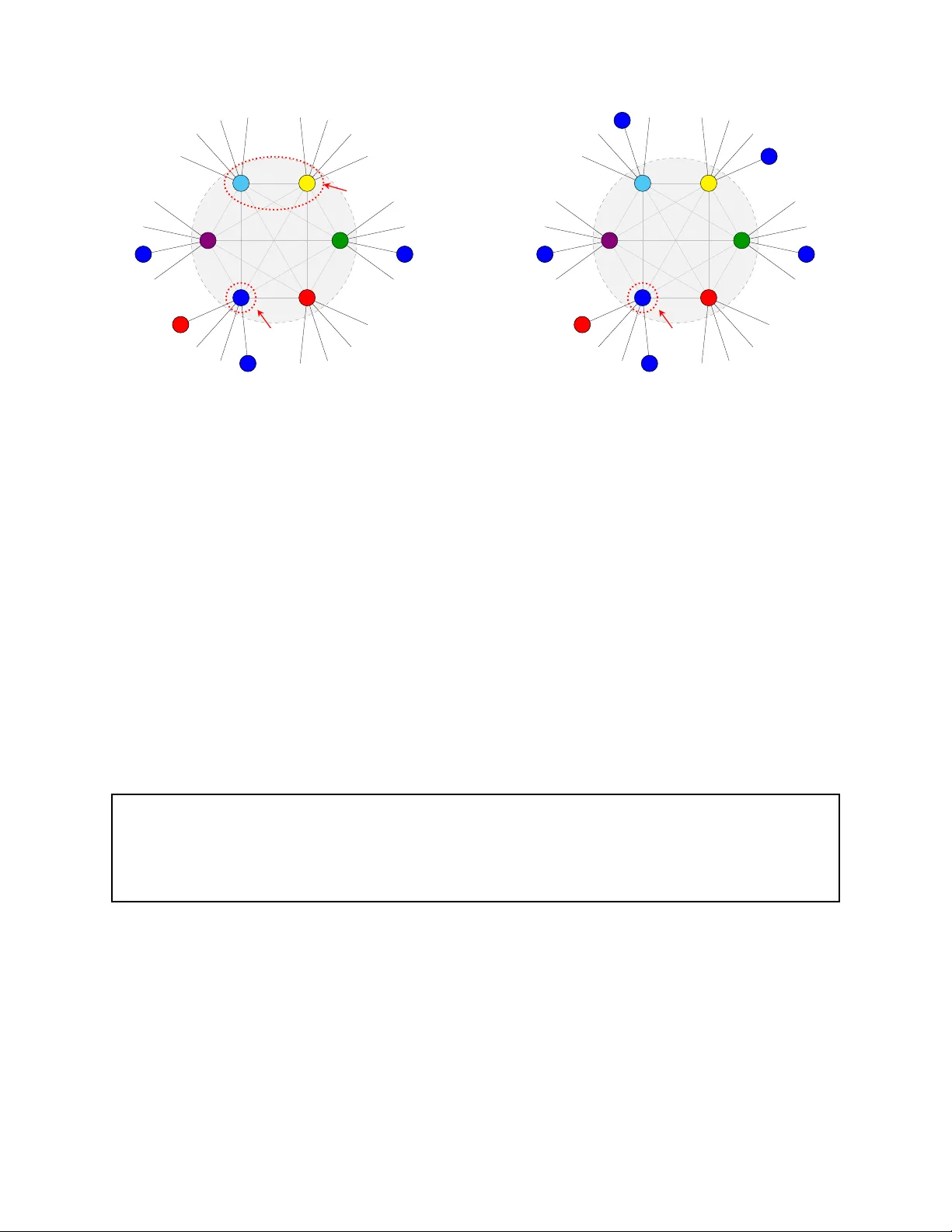
Sublogarithmic Distributed V ertex Coloring with Optimal Num b er of Colors Maxime Flin ∗ Aalto Univ ersity maxime.ﬂin@aalto.ﬁ Magn ´ us M. Halld´ orsson † Reykja vik Universit y mmh@ru.is Man uel Jakob ‡ TU Graz m.jak ob@tugraz.at Y annic Maus ‡ TU Graz y annic.maus@tugraz.at Abstract F or any ∆, let k ∆ b e the maxim um integer k suc h that ( k + 1)( k + 2) ⩽ ∆. W e give a distributed LOCAL algorithm that, given an in teger k < k ∆ , computes a v alid ∆ − k -coloring if one exists. The algorithm runs in e O ( log 4 log n ) rounds, whic h is within a polynomial factor of the Ω( log log n ) low er bound, whic h already applies to the case k = 0. It is also b est p ossible in the sense that if k ⩾ k ∆ , the problem requires Ω( n/ ∆) distributed rounds [Molloy , Reed, ’14, Bamas, Esp eret ’19]. F or ∆ at most p olylogarithmic, the algorithm is an exp onen tial improv ement ov er the curren t state of the art of O ( log 49 / 12 n ) rounds. When ∆ ⩾ ( log n ) 50 , our algorithm achiev es an even faster run time of O (log ∗ n ) rounds. ∗ This work was supp orted in part b y the Research Council of Finland, Grants 359104 and 363558. Part of this w ork w as done while the author was working at Reykjavik Univ ersity , funded b y the Icelandic Research F und, Gran t 2310015-053. † Supp orted b y the Icelandic Research F und, Grant 2511609. ‡ This research was funded in whole or in part by the Austrian Science F und (FWF) https://doi.org/10.55776/ P36280 , https://doi.org/10.55776/I6915 . F or op en access purp oses, the author has applied a CC BY public cop yright license to any author-accepted manuscript version arising from this submission. Con ten ts 1 In tro duction 1 1.1 F urther Background on Distributed Graph Coloring . . . . . . . . . . . . . . . . . . 2 1.2 The Challenges and Our T echnical Con tributions . . . . . . . . . . . . . . . . . . . . 3 1.3 Organization of the Paper . . . . . . . . . . . . . . . . . . . . . . . . . . . . . . . . . 5 2 T ec hnical Ov erview 5 2.1 Color Co verage (CC) & Π-ous subgraphs . . . . . . . . . . . . . . . . . . . . . . . . 5 2.2 Ov erview of the Coloring Algorithm . . . . . . . . . . . . . . . . . . . . . . . . . . . 7 2.3 Smaller Degrees and the Lov´ asz Lo cal Lemma . . . . . . . . . . . . . . . . . . . . . . 8 3 Preliminaries 10 3.1 Lo v´ asz Lo cal Lemma . . . . . . . . . . . . . . . . . . . . . . . . . . . . . . . . . . . . 11 3.2 Our Shattering F ramework . . . . . . . . . . . . . . . . . . . . . . . . . . . . . . . . 11 4 T op-Lev el Algorithm and Pro ofs of Theorems 1 and 2 14 4.1 Graph Decomp osition . . . . . . . . . . . . . . . . . . . . . . . . . . . . . . . . . . . 14 4.2 The Color Cov erage (CC) Prop ert y . . . . . . . . . . . . . . . . . . . . . . . . . . . . 15 4.3 F ull Algorithm and Pro ofs of Theorems 1 and 2 . . . . . . . . . . . . . . . . . . . . . 16 5 Coloring With Muc h Slack 19 5.1 Iterated Random Color T rial with Prop ert y CC ( Lemma 5.1 ) . . . . . . . . . . . . . 20 5.2 Finishing Oﬀ The Coloring via MCT (Lemma 5.2 ) . . . . . . . . . . . . . . . . . . . 24 6 Coloring the Sparse No des 26 6.1 Algorithm for Sparse No des . . . . . . . . . . . . . . . . . . . . . . . . . . . . . . . . 26 6.2 Degree Splitting (Pro of of Lemma 6.3 ) . . . . . . . . . . . . . . . . . . . . . . . . . . 28 6.3 Slac k Generation (Pro of of Lemma 6.1 ) . . . . . . . . . . . . . . . . . . . . . . . . . 31 7 Coloring Cliques 35 7.1 Step 1: Sync hronized Color T rial . . . . . . . . . . . . . . . . . . . . . . . . . . . . . 35 7.2 Step 2: Finding Safe Swaps . . . . . . . . . . . . . . . . . . . . . . . . . . . . . . . . 36 7.3 Step 3: Lo cal Matching . . . . . . . . . . . . . . . . . . . . . . . . . . . . . . . . . . 37 7.4 Pro of of Lemma 7.2 . . . . . . . . . . . . . . . . . . . . . . . . . . . . . . . . . . . . 38 7.5 Pro of of Lemma 7.6 . . . . . . . . . . . . . . . . . . . . . . . . . . . . . . . . . . . . 40 8 Ultrafast Coloring High-Degree Graphs 45 A Graph Decomp osition by Molloy-Reed 51 B Concentration Inequalities 53 C Slac k Generation 54 ii 1 In troduction Graph coloring is a problem of fundamen tal imp ortance to com binatorics and computer science. Giv en a graph G = ( V , E ) and an in teger c ⩾ 1, a c -coloring of G is a mapping from the vertices of G to { 1 , 2 , . . . , c } suc h that adjacen t v ertices of G receiv e diﬀerent colors. Determining the smallest c for which a giv en graph admits a c -coloring – a v alue kno wn as the chromatic n umber denoted by χ ( G ) – has b een an enduring challenge in graph theory since its v ery b eginning. Computationally , it has long b een known that computing exactly or even appro ximately the chromatic num b er of a graph is NP-hard [ Kar72 ; Zuc07 ]. In general, the chromatic num b er of a graph dep ends on the global structure of the graph rather than on purely lo cal prop erties (see [ AS00 , Chapter 3]). Distributed Graph Coloring. In the LOCAL mo del, introduced by Linial [ Lin92 ], the input graph G is seen as a netw ork in which n = | V | no des equipp ed with unique identiﬁers communicate with their neighbors in synchronous rounds and p erform unlimited lo cal computation, aiming to minimize the total n umber of rounds until each no de has computed its output, e.g., its color in a graph coloring problem. In this setting, one classically aims to compute a ∆ + 1-coloring where ∆ is the maxim um degree of the graph [ BE13 ]. Sequentially , the problem is trivial as one can greedily assign colors to no des without ev er getting stuck, or in other w ords, any v alid partial coloring can alw ays b e completed to a coloring of the whole graph. Essentially all eﬃcien t distributed graph coloring algorithms exploit this greedy b ehavior of the problem, e.g., [ BEPS16 ; CLP20 ; MT20 ; GK21 ; HKNT22 ; GG24 ]. The most imp ortan t exceptions are sev eral pap ers that aim for an eﬃcien t distributed implementation of Bro oks’ theorem [ Bro41 ] for coloring w ith exactly ∆ colors, e.g., [ PS95 ; GHKM18 ; FHM23 ; HM24 ; BBN26 ; BBN25 ]. Coloring with F ew er Colors. Coloring graphs whose chromatic n umber is smaller than ∆ using the optimal n umber of colors is challenging, even in the centralized setting. In a seminal pap er, Molloy and Reed [ MR14 ] characterized the precise threshold at whic h the problem b ecomes NP-complete. Let k ∆ b e the largest integer such that ( k ∆ + 1)( k ∆ + 2) ⩽ ∆. 1 They sho wed that for c < ∆ − k ∆ the decision problem whether a graph admits a c -coloring is NP-complete, while for c ⩾ ∆ − k ∆ the decision is based on whether the induced neighborho o d G [ N [ v ]] of some no de v is c -colorable. F urthermore, for c ⩾ ∆ − k ∆ the coloring can b e computed b y a (centralized) p olynomial-time algorithm when ∆ is a constan t. This result is highly non-trivial, spanning more than 60 dense pages [ MR14 ]. In the distributed setting, Bamas and Esp eret sho w ed that for c = ∆ − k ∆ computing a c -coloring of a graph with c hromatic num b er c requires Ω( n/ ∆) rounds [ BE19 ]. Based on the work of Molloy and Reed, they also gav e a randomized algorithm for the LOCAL mo del to c -color graphs when c > ∆ − k ∆ in a p olylogarithmic num b er of rounds. In con trast, the state-of-the-art algorithms for (∆ + 1)-coloring and, recently also for ∆-coloring, only require p oly ( log log n ) randomized distributed time [ CLP20 ; RG20 ; GHKM18 ; FHM23 ; BBN25 ]. This discrepancy motiv ates the follo wing question. Can one c olor in a sublo garithmic numb er of r ounds with fewer than ∆ c olors? Our Results. In this pap er, we answer the question in the aﬃrmativ e. W e show that one can compute a c -coloring in sublogarithmic time when one exists and c ⩾ ∆ − k ∆ + 1. Moreov er, when ∆ is asymptotically larger than some p olylogarithm in n , our algorithm runs in O ( log ∗ n ) rounds, matc hing the state of the art for the signiﬁcantly easier (∆ + 1)-coloring problem. More precisely , w e prov e the following theorem: 1 It can b e veriﬁed that k ∆ = ⌊ p ∆ + 1 / 4 − 3 / 2 ⌋ and thus √ ∆ − 3 < k ∆ < √ ∆ − 1 holds. 1 Theorem 1. F or suﬃciently lar ge ∆ , and any c ⩾ ∆ − k ∆ + 1 , ther e is a distribute d r andomize d algorithm that takes a gr aph G with maximum de gr e e ∆ as input, and do es the fol lowing: either some vertex outputs a c ertiﬁc ate that G is not c -c olor able, or the algorithm ﬁnds a c -c oloring of G . The algorithm runs in O ( log ∗ n ) r ounds when ∆ ⩾ ( log n ) 50 , and in gener al in e O ( log 4 log n ) r ounds 2 , with high pr ob ability. Theorem 1 comes p olynomially close to the low er b ound of Ω( log ∆ log n ) rounds established for the ∆-coloring problem [ BFHKLRSU16 ]. Moreov er, this result uses the fewest n umber of colors p ossible due to the aforemen tioned low er b ound from [ BE19 ]. While our approac h builds on the framew ork of Molloy and Reed, it is conceptually and tec hnically simpler in several key asp ects; see Sections 1.2 and 2 for details. By plugging the randomized algorithm from Theorem 1 in to the p o w erful distributed derandom- ization framework of [ GKM17 ; GHK18 ; RG20 ; GG24 ] w e obtain more than a quadratic improv emen t for deterministic algorithms. Previously the b est algorithm, using state-of-the-art subroutines [ GG24 ; R G20 ], had complexit y O (log 49 / 12 n ) [ BE19 ]. Theorem 2. F or suﬃciently lar ge ∆ , and any c ⩾ ∆ − k ∆ + 1 , ther e is a distribute d deterministic algorithm that takes a gr aph G with maximum de gr e e ∆ as input, and do es the fol lowing: either some vertex outputs a c ertiﬁc ate that G is not c -c olor able, or the algorithm ﬁnds a c -c oloring of G . The algorithm runs in e O (log 2 n ) r ounds. The run time of Theorem 2 is only roughly quadratically slow er than the low er b ound of Ω( log ∆ n ) rounds established for the ∆-coloring problem [ CKP16 ] and almost matches the natural barrier of Ω( log 2 n ) rounds for the deterministic complexit y of the problem. Surpassing it is b eliev ed to require fundamen tally new techniques. Molloy and Reed’s, Bamas and Esp eret’s, and also our algorithm for computing a coloring with fewer than ∆ colors rely in multiple places on solving instances of the constructiv e Lov´ asz Lo cal Lemma (LLL). The only kno wn metho d to do this deterministically in a distributed setting is via the aforemen tioned derandomization framework that inherently comes with an Ω( log 2 n ) cost; see [ GG24 ] for more details. Breaking this barrier for general LLLs is considered one of the biggest op en problems in the ﬁeld. Chang and P ettie conjectured in [ CP19 ] that this can b e done on b ounded-degree graphs, but this question remains unansw ered. 1.1 F urther Background on Distributed Graph Coloring Historic fo cus on Greedy problems. Coloring was the central topic of the pap er e stablishing the LOCAL mo del [ Lin92 ]. How ever, since this mo del requires that no des decide on their colors only based on their lo cal view, ev en solving greedy problems such as maximal indep enden t set, maximal matc hing or (∆ + 1)-vertex-coloring is highly non-trivial. Linial show ed that ev en coloring an n -cycle with a constan t num b er of colors requires at least Ω( log ∗ n ) rounds for deterministic algorithms and Naor later extended this low er b ound to the randomized setting [ Nao91 ]. It to ok roughly 30 y ears to understand that on general graphs those greedy problems could b e solv ed deterministically in p olylogarithmic distributed time thanks to a breakthrough b y Rohzon and Ghaﬀari [ R G20 ]. Over the last 5 y ears, follow-up w ork [ GK21 ; BBHORS21 ; FGGKR23 ; GG24 ] on deterministic algorithms coupled with earlier randomized tec hniques [ BEPS16 ; Gha16 ; CLP20 ; HKNT22 ] led to exciting progress on our understanding of the complexity of greedy problems in the LOCAL mo del. Recen t in terest in the lo calit y of non-greedy problems. 3 Despite rising interest in the lo calit y of non-greedy problems, e.g., for the seminal w orks on (h yp ergraph) sinkless orientation 2 In this pap er, e O ( f ( n )) hides m ultiplicative factors of size poly log f ( n ). 3 In tuitively , a non-greedy problem is one where not every partial solution can b e extended to a full solution. One 2 problems [ BFHKLRSU16 ; GS ; BMNSU25 ], for v arious degree splitting problems [ GHKMSU17 ; HMN22 ; Da v23 ], and for the more amenable non-greedy edge coloring problems, e.g., [ GKMU18 ; SV19 ; HN21 ; HMN22 ; CHLPU20 ; Dav23 ; JMS25 ], little is known for non-greedy vertex coloring. The exception is the aforementioned coloring with exactly ∆ colors. A well-kno wn theorem of Bro oks [ Bro41 ] shows that an y connected graph admits a ∆-coloring unless it is a (∆ + 1)-clique or an o dd cycle. There hav e b een several w orks designing faster and faster algorithms for the problem [ PS95 ; GHKM18 ; FHM23 ; HM24 ; BBN25 ] culminating in the very recent result of [ BBN26 ] obtaining an optimal round complexit y when ∆ = O (1). The only kno wn works attempting to color with fewer than ∆ c olors are for v ery sparse graphs, i.e., triangle-free graphs [ CPS17 ], but their randomized complexities remain at least logarithmic. In a diﬀerent direction, Barenboim designed a randomized distributed algorithm that computes an O ( n 1 / 2+ ε χ ( G ))-coloring of any graph G [ Bar12 ]. The imp ortance of the Lo v´ asz Lo cal Lemma. The Lov´ asz Lo cal Lemma (LLL) provides a p o w erful probabilistic framework for showing that, ev en when many lo cal bad even ts may o ccur, there exists a global conﬁguration that a voids all of them simultaneously . Informally , it can b e view ed as a lo calized analogue of the union b ound: if each bad even t o ccurs with suﬃciently small probabilit y and dep ends on only a limited n umber of other even ts, then one can still guarantee the existence of an outcome in which no bad ev ent o ccurs. In the c onstructive v ersion of the LLL, the goal is not only to prov e existence but also to eﬃciently compute suc h an ass ignmen t. Mollo y and Reed’s algorithm for coloring with c ⩾ ∆ − k ∆ hea vily relies on multiple instances of the constructive LLL (see Section 11 in [ MR14 ]). In essence, the LLL is used to ensure that partial colorings retain prop erties similar to those of a random coloring, thereby guaranteeing that they can alw ays b e extended without creating deadlo c ks. In their distributed adaptation, Bamas and Esp eret signiﬁcantly reduced the n umber of required LLL instances and solved eac h of them using a logarithmic-time distributed LLL solver based on the Moser–T ardos framew ork [ BE19 ; MT10 ; CPS17 ]. T o date, no non–LLL-based approach is kno wn for computing such colorings. In the distributed setting, random v ariables and bad even ts are naturally asso ciated with no des of the communication netw ork, and the ob jective mirrors that of the constructive LLL: to compute a global assignmen t that av oids all bad ev ents. Consequen tly , understanding the distributed complexit y of the LLL has b ecome a cen tral challenge in the ﬁeld. In a seminal result, Chang and Pettie [ CP19 ] sho wed that the LLL is complete for sublogarithmic-time computation of lo cal graph problems on constan t-degree graphs. As a consequence, any such problem with sublogarithmic complexit y can b e solv ed in p oly ( log log n ) rounds using the distributed LLL algorithm of Fischer and Ghaﬀari [ FG17 ]. F or general graphs, how ever, it remains a ma jor op en question which problems admit sublogarithmic- time distributed algorithms. The complexity of the general distributed LLL on general graphs is also widely op en, despite recent progress on sp ecial cases [ GHK18 ; Dav23 ] and results showing sublogarithmic a verage-time complexity p er node [ Da v25 ]. Moreo ver, the constructive LLL admits an Ω( log log n ) randomized lo wer bound [ BFHKLRSU16 ]. Our work not only yields sublogarithmic-time algorithms for coloring with few er than ∆ colors, but also provides sublogarithmic-time solutions for sev eral LLL instances that, prior to our work, w ere only known to admit logarithmic-time distributed solutions. 1.2 The Challenges and Our T echnical Con tributions Our approach follows the same high-level structure as that of Molloy and Reed [ MR14 ]. As in their w ork, w e ﬁrst transform the input graph to exp ose its structural regularities and then decomp ose it distinguishing feature is that greedy problems can b e solved in O ( log ∗ n ) rounds on constant-degree graphs, while non-greedy problems require at least Ω(log log n ) rounds. See [ JMS25 ] for a more formal discussion on the topic. 3 in to ﬁv e comp onents: a sparse region, t wo dense regions consisting of cliques, and t wo intermediate regions linking them. These comp onen ts are colored in a carefully chosen order while main taining probabilistic in v arian ts that guarantee that the dense cliques can b e completed in the ﬁnal stages. W e refer to Section 2 for a more detailed ov erview of this framework. Challenges in achieving sublogarithmic distributed algorithms. While the Molloy–Reed framew ork provides a conceptually clean approac h, several asp ects p ose ma jor c hallenges in the distributed setting: 1. The metho d of [ MR14 ] for coloring the sparse and intermediate regions relies on an iterative semi-random pro cess. This pro cedure is tec hnically inv olv ed—requiring a lengthy analysis—and inheren tly slow, as it p erforms ∆ Θ(1) iterations, each requiring the solution of an LLL instance. Although Bamas and Esp eret reduced this to O ( log 13 / 12 ∆) ite rations, this complexity remains far to o large for ac hieving sublogarithmic distributed time. 2. The probabilistic arguments throughout [ MR14 ] are based on the Lo v´ asz Lo cal Lemma. Kno wn distributed LLL solvers require Ω( log n ) rounds in general [ BE19 ; MT10 ; CPS17 ]. While some LLL instances can b e solved faster when the criteria are suﬃciently relaxed [ HMN22 ; Dav23 ], others – most notably those arising from the dense regions – satisfy only p olynomial LLL criteria and thus resist existing fast techniques. As a consequence, a direct distributed implementation of the Molloy–Reed framework inevitably leads to high round complexit y . Notably , this diﬃculty is most pronounced for high-degree graphs, despite the fact that such graphs admit ultrafast distributed algorithms for simpler problems such as ∆-coloring [ FHM23 ]. Our Contributions. W e present a sublogarithmic-time distributed algorithm for coloring with ∆ − k ∆ + 1 colors b y reﬁning and simplifying the Mollo y–Reed framework. 1. A central slack in v ariant. Our main conceptual contribution is the introduction of a central in v ariant based on slack , ensuring that each vertex consistently has more a v ailable colors than comp eting constraints. The k ey feature of this inv arian t is its monotonicity: as the algorithm progresses, the loss of av ailable colors is matched by a corresp onding reduction in uncolored neigh b ors, so that slack do es not deteriorate. This viewp oin t allows us to a void tracking the detailed evolution of color lists and degrees o ver time. Rather than carefully con trolling distributions at each step, we rely on the in v ariant to ensure that partial colorings remain extendable, leading to a simpler and more robust approac h to coloring the sparse and intermediate regions. 2. F aster handling of structured LLL instances. W e develop sublogarithmic-time solutions for the Lov´ asz Lo cal Lemma instances arising in our setting. Our approach builds on the shattering framew ork, augmented with additional mec hanisms—such as guard even ts—that ensure the residual instances remain well-behav ed and av oid cascading dep endencies. While the individual ingredients ha ve app eared in prior work, their combination allows us to handle LLL instances that w ere not previously known to admit such fast distributed solutions. 3. P arallel coloring of dense cliques. F or dense regions, we introduce a subsampling technique that enables cliques to b e colored in parallel b y reducing the problem to indep enden t matc hing tasks within each clique. This av oids the need for global co ordination and simpliﬁes the treatmen t of dense structures compared to prior approaches. 4 4. Ultrafast algorithms in the high-degree regime. In graphs of suﬃciently large degree, we can replace the core iterativ e coloring step with a reduction to a form of list coloring that admits v ery fast distributed algorithms. As all our probabilistic claims hold with sub exp onen tial error b ounds, we also bypass the application of LLL altogether. This leads to a O ( log ∗ n )-time solution when ∆ ⩾ log 50 n . Conceptually , our results expand the small but growing class of explicit distributed LLL form ulations that can b e solv ed in sublogarithmic time on general graphs. Despite this progress, designing a general distributed LLL algorithm that eﬃciently handles all relev an t instances across all degree regimes remains a ma jor op en problem in the ﬁeld. 1.3 Organization of the P ap er In Section 2 , w e present the main technical ideas underlying our approac h, while Section 3 contains complemen tary background material. The algorithm is describ ed formally in Section 4 , where we also pro ve Theorems 1 and 2 . The subroutines and their analyses for coloring Π-ous subgraphs, sparse v ertices, and dense vertices are presented in Sections 5 to 7 , resp ectiv ely . The high-degree case is treated separately in Section 8 . The substantial technical detail throughout the pap er is driven by the goal of achieving sublog- arithmic distributed run time. If one w ere only concerned with the existence of such colorings, a p olynomial-time cen tralized algorithm, or a p olylogarithmic-time distributed solution, many sections could b e signiﬁcantly simpliﬁed. 2 T ec hnical Overview W e give an ov erview of the main technical ideas b ehind Theorem 1 , fo cusing on ho w to construct a (∆ − k ∆ + 1)-coloring in sublogarithmic distributed time. In Section 2.3 , w e attempt to give a bird’s ey e view of the tec hniques allowing us to solv e each instance of the Lov´ asz Lo cal Lemma in sublogarithmic time. 2.1 Color Co v erage (CC) & Π -ous subgraphs Due to the imp ossibilit y of completing all partial solutions in a non-greedy coloring problem, the hardest part of the problem is coloring the last v ertices. In a non-greedy coloring problem, one has to construct a coloring while ensuring that the remaining no des can b e colored later. F ollowing Mollo y and Reed, w e color the dense vertices last and b egin by reviewing the conditions necessary for coloring the cliques at the end. Color Swapping in Cliques. Consider a (∆ − k ∆ + 1)-clique in which every vertex is adjacent to k ∆ no des outside the clique and all but one vertex hav e b een prop erly colored. T o color this remaining vertex v , which we call unhappy , Molloy and Reed swap its color with that of some other v ertex in the clique. In order to do so without creating new conﬂicts, the vertex u with which v sw aps its color must ha ve no external neighbors with v ’s color (and vice versa). See Figure 1a . Ho wev er, it may happ en that the coloring outside the clique do es not p ermit any such swap (as in Figure 1b ). T o circumv ent this issue, Molloy and Reed constrain all earlier steps of the coloring algorithm so that the coloring outside eac h clique b eha ves suﬃcien tly randomly . Concretely , this means that for every clique and every color, only a small num b er of v ertices are forbidden from using that color. W e formalize this requirement as the c olor c over age (henc eforth CC) pr op erty . Ensuring that CC holds until coloring the dense parts of the graph is essential to completing the coloring. See 5 A i Swappable unhappy (a) A i unhappy (b) Figure 1: A clique A i in a graph with ∆ = 9 and k = 3. On Figure 1a , the clique A i con tains one unhapp y vertex, in blue. It c annot swap its color with the purple or green v ertex b ecause they hav e a blue external neigh b or. It cannot swap its color with the red vertex b ecause it has a red external neigh b or. The remaining v ertices (in cyan and yello w) mak e the Sw appable set for this unhapp y v ertex. On Figure 1b , the Sw appable set is empty b ecause to o many vertices on the outside adopted the blue color. Section 4.2 for the precise deﬁnition of CC. Π -ous subgraphs. The CC condition can b e main tained if all earlier coloring steps are suﬃcien tly random. If eac h dense no de has at most U neigh b ors outside its clique, and each of them picks one random color out of U · ∆ 0 . 22 colors, then few of these outside neighbors pick the same color, thereb y maintaining the CC condition. Th us, the k ey to ensuring the CC condition in eac h step of the algorithm is to main tain large lists of av ailable colors L ( v ) (colors that do not currently app ear in the neighborho o d of v ) compared to the n umber of outside neighbors of the cliques. W e capture this condition through Prop ert y Π , which we state in a simpliﬁed form as follows: Prop ert y Π (formalized in Section 4.3 ). A n induc e d sub gr aph H satisﬁes Pr op erty Π if (a) e ach unc olor e d dense vertex has at most U outside neighb ors, and (b) e ach vertex u ∈ H has a list L ( u ) of at le ast d H ( u ) + U · ∆ 0 . 22 available c olors. In tuitively , Prop erty Π guarantees that every vertex has enough slac k compared to the num b er of neigh b ors outside its dense structure. Subgraphs satisfying Prop erty Π are called Π -ous (pronounced pi ous). W e can color a Π-ous subgraph H while maintaining CC by a combination of iterated random color trials ( R ct ) and m ulti color trials ( Mct ). Condition (b) of Prop erty Π ensures that the list of av ailable colors for eac h vertex of H has U · ∆ 0 . 22 slack that remains and ensures a suﬃcien tly large list regardless of ho w the coloring of H pro ceeds. Slac k do es not decrease b ecause coloring a neigh b or remo ves b oth one comp eting vertex and one a v ailable color, lea ving their diﬀerence—the slac k—unchanged or increased. 6 Prop ert y Π is strictly stronger than assumptions of [ MR14 ]. Their assumption (8.2) on the list size inv olv es a max of t wo terms, not the sum, whic h means that slack is only guaran teed when degrees are high. 2.2 Ov erview of the Coloring Algorithm Our algorithm centers on identifying Π-ous subgraphs that can b e colored while main taining Prop ert y CC , thereb y ensuring that the dense vertices can b e colored last. W e build on the structural decomp osition of Molloy and Reed, whic h nearly 4 partitions the sparser regions of the graph into Π-ous subgraphs [ MR14 ]. More precisely , they reduced the problem of ﬁnding a c -coloring of G to the problem of ﬁnding a c -coloring of a graph F with a very sp eciﬁc structure. Bamas and Esp eret also show ed that F can b e constructed from G in O (1) rounds in the LOCAL mo del, and that one can eﬃciently recov er a c -coloring of G from a c -coloring of F in the distributed setting [ BE19 ]. Structural Decomp osition (formalized in Lemma 4.1 ). The vertices of the graph F are partitioned in to ﬁve sets as follo ws: • Sparse v ertices ( S ): vertices whose neighborho o ds are far from b eing cliques, either ha ving noticeably low er degree or many missing edges among their neighbors, • High-slac k intermediates ( B H ): v ertices outside the cliques that ha ve many neighbors in cliques, • Cliques with large external degree ( A H ): true cliques of size b et ween c − Θ( √ ∆ ) and c and whose vertices hav e at most O ( √ ∆) external neighbors, • Lo w-slack in termediates ( B L ): v ertices that still ha ve many neigh b ors in cliques, but not as many as the vertices in B H , • Cliques with small external degree ( A L ): the ﬁnal cliques to b e colored, each with ev en smaller external degree b ounded by O (∆ 1 / 4 ). While we follow the same o verall structure as Molloy and Reed’s algorithm, the internal comp onen ts diﬀer signiﬁcantly . Most notably , the fact that w e aim to color Π-ous subgraphs means that w e can use a simpler analysis. First, w e observe that B H and B L are Π-ous b y deﬁnition; w e then provide a simple metho d to partition S in to tw o Π-ous subgraphs; and ﬁnally design a highly parallelizable approac h for coloring the cliques. Coloring S, B H and B L is one of the most tec hnically inv olv ed parts in [ MR14 ]. W e shortly detail each of these steps. Coloring no des in B H and B L . By construction, no des in B H and B L ha ve many uncolored neigh b ors in cliques, whic h provides them with temp orary slack; as a result, they satisfy Prop ert y Π purely due to structural prop erties. It is crucial that the v ertices in B L are colored after the cliques in A H . Although lists of v ertices in B L are guaran teed to hav e size Ω( √ ∆ ), this is insuﬃcient for B L b eing Π-ous if A H is still uncolored. Coloring the Sparse V ertices in S . It is well known that a single round of random color trials ( R ct ) gives each v ertex v ∈ S slac k Ω( √ ∆ ). This pro cess is called slack generation. Unfortunately , 4 The subgraphs induced b y B H and B L are Π-ous b y construction, how ever the subgraph induced by S is not Π-ous right a wa y; see Section 6 for more details. 7 A i Al l i B S Figure 2: A schematic illustration of the structural decomp osition by Molloy and Reed. The v ertices of S are lo osely connected, while the set A i is a clique. The intermediate set B is to o highly connected to A to b e considered sparse, but not densely enough to b e itself part of the clique. F or the coloring, w e further divide the set B in to tw o subsets, B H and B L (see Lemma 4.1 ); ho wev er, the ﬁgure shows B as a single set for simplicit y . Note that some vertices of B , here in the set All i , can b e connected to all the vertices of a clique (see Lemma 4.1 for details on the set Al l i ). this is still insuﬃcient for Prop ert y Π requiring slac k U · ∆ 0 . 22 where U = Θ( √ ∆ ). W e therefore split the remaining uncolored vertices S ′ in to tw o groups S 1 and S 2 . Coloring S 1 ﬁrst gives their v ertices extra temp orary slack (from neighbors in S 2 ), and when we color S 2 w e can rely on the fact that dense vertices hav e few neigh b ors in S 2 making it easier to satisfy Prop ert y Π . Coloring of Cliques. T o ac hieve a sublogarithmic distributed runtime, we color cliques in A H and A L resp ectiv ely in parallel. F or each clique A i , w e assign a random p ermutation of the colors to its v ertices av oiding any conﬂicts inside the clique. With this pro cess, only O ( √ ∆ ) v ertices p er clique conﬂict with external neighbors. Each such unhappy vertex v seeks a partner u in A i so that b oth b ecome happy if they swap their colors. Prop ert y CC crucially guaran tees a large supply of v alid swap candidates. T o execute swaps in all cliques concurrently , w e ﬁrst indep enden tly do wnsample the candidate sets and remo ve those causing external c onﬂicts , i.e., swaps that cannot b e executed safely in parallel with sampled candidate swaps in adjacent cliques. W e sho w that, after this pruning step, suﬃciently man y candidates remain to also a void internal c onﬂicts . W e set up a bipartite graph b et ween unhappy vertices and their remaining candidates and sho w that it satisﬁes Hall’s condition, ensuring a p erfect matching b etw een unhappy no des and swap candidates. W e can then p erform the corresp onding swaps sim ultaneously without in terference within the clique and due to the prior pruning also without interference b et ween diﬀerent cliques. 2.3 Smaller Degrees and the Lo v´ asz Lo cal Lemma All steps of our coloring algorithm are randomized and hav e a lo cal failure probability of the form exp ( − ∆ ε ) for some univ ersal constant ε ∈ (0 , 1]. Hence, when ∆ ≫ log 1 /ε n , our algorithm succeeds with high probability . How ev er, when ∆ ⩽ p oly(log n ), lo cal failures can no longer b e a voided. The main tool at our disp osal to handle lo cal failures is the Lo v´ asz Lo cal Lemma. Since w e aim for a sublogarithmic runtime, we cannot rely on the general framework by Moser and T ardos [ MT10 ; CPS17 ]. The only general approach currently kno wn to achiev e sublogarithmic round complexit y is the shattering fr amework [ BEPS16 ]. Unfortunately , there exists no general-purp ose distributed LLL solver yielding sublogarithmic time on graphs of all degrees, in particular in the 8 c hallenging regime where degrees are sublogarithmic but exceed p oly ( log log n ). 5 F or v ery low degree graphs, sublogarithmic-time algorithms are known [ FG17 ; Dav23 ]. W e therefore design dedicated constructions tailored to the diﬀerent degree regimes. The Shattering F ramework. In this framework, a fast, randomized pr e-shattering phase resolves most of the graph – for instance, ﬁxing the colors of the ma jority of vertices – leaving only small residual comp onen ts of size p oly ( log n ). A subsequen t p ost-shattering phase then deterministically completes the solution b y solving a smaller residual LLL problem, typically within p oly ( log log n ) rounds. As one randomly colors v ertices in the pre-shattering phase, one may be forced to uncolor certain v ertices. F or instance, if a color app ears to o frequen tly around a clique and Prop ert y CC is violated. This may in terfere with the progress measures of our algorithm, which are typically form ulated as additional bad even ts. F or instance, uncoloring vertices ma y violate an ev ent ensuring a constant-factor decrease in the uncolored degree. Such even ts are usually resolv ed during the p ost-shattering phase. The k ey challenge, especially for non-greedy problems such as ours, is to design the pre-shattering phase in suc h a wa y that the p ost-shattering instance (1) is solv able and (2) has p olylogarithmic size comp onen ts, meaning that retractions (e.g., uncolorings) do not p ercolate to the large parts of the graph. W e introduce several metho ds to deal with these challenges. • F r esh budgets are used in the pre-shattering and the p ost-shattering whenev er we do not w ant to see to o many of something. By giving half of the total budget to eac h of the shattering steps, w e remov e the dep endencies b et w een the t wo phases. • Mar ginal events are added in the p ost-shattering phase to accoun t for previously av oided bad ev ents that could b e reactiv ated b y newly assigned v ariables. • Guar d events imp ose additional constraints to preserve suﬃcient randomness for the p ost- shattering phase. They prev ent the pre-shattering pro cess from ﬁxing to o many v ariables or o vercommitting to sp eciﬁc random outcomes, which would reduce the av ailable randomness needed later. • Palette splitting further separates randomness b etw een pre- and p ost-shattering: one part of the color palette is used in pre-shattering, the other in p ost-shattering. Despite this restriction, the probabilistic guarantees of each step contin ue to hold. Example 1: Subsampling Swap Candidates. T o illustrate those t wo ideas, consider the LLL that gov erns subsampling of swap candidates in cliques. Each unhappy v ertex v indep enden tly samples p oten tial partners with a ﬁxed probabilit y; with o verwhelming probability , ev ery vertex obtains suﬃcien tly many candidates. The subtlet y lies in showing that, after pruning candidates in volv ed in conﬂicting swaps across adjacen t cliques, enough v alid partners remain. This is ac hiev able, and the shattering analysis ensures that the comp onen ts where the sampling fails are small. Since we only pick candidates in pre- and p ost-shattering using separate budgets, this increases the num b er of neigh b ors with a giv en color by a factor of at most tw o compared to ha ving one single budget for b oth steps. Con venien tly , the same analysis b ounds the probability of breaking Prop ert y CC for the pre- and p ost-shattering. Remo ving candidates do es not make other candidates bad, how ev er, resampling candidates to repair lo cal failures can aﬀect neighboring cliques, and p otentially undo the progress made during pre-shattering. T o resolve this, w e add an even t in p ost-shattering for each clique adjacent to some 5 W e cannot pro v ably rule out that some of our LLLs could b e solved via the sublogarithmic-time algorithm of [ GHK18 ], but we do not kno w how to prov e that they fall into the handled class of LLLs either. 9 other clique that resamples its candidates in p ost-shattering. Example 2: Slac k Generation. T o illustrate the latter t wo techniques, let us lo ok at the slac k generation LLL. Sparse no des ha ve man y non-edges in their neigh b orho od, i.e., pairs of non-adjacent no des. One can show that one round of random color trials pro vides a no de with slack prop ortional to the n umber of non-edges by same-coloring the endp oints of man y of these non-edges. One can sho w that receiving suﬃcien t slack forms an LLL. In a pre-shattering phase based on randomly coloring vertices, a no de ma y also obtain to o little slac k. No w, if all of its neigh b ors are already colored, it is impossible for it to obtain slack in the p ost-shattering phase. Uncoloring its neighbors would remov e the slack of other no des and in fact this ma y p ercolate through the graph. Instead, we use a guarding even t that ensures that in the pre-shattering phase few enough neigh b ors of eac h no de participate in the coloring pro cedure ensuring that enough neighbors (and also non-edges b et w een them) remain uncolored for a tentativ e p ost-shattering phase. Of course, this ev ent can also fail but one can verify that the guarding even t prev ents p ercolation of uncolorings. If enough neighbors (and also non-edges b et ween them) remain uncolored in p ost-shattering, w e can use the same random pro cess with a disjoint palette to decouple the randomness of the pre-shattering and p ost-shattering phase. The Quest for a Sublogarithmic LLL F ramework. W e solve se v eral LLLs b y a combination of the mitigations ab o ve. Developing a general black-box framework that can solv e all distributed LLLs of this form in sublogarithmic time remains an op en challenge. Determining precisely whic h classes of LLL instances admit such runtimes is, in our view, one of the central op en problems in the distributed complexity of the Lov´ asz Lo cal Lemma. Op en Problem 1. Do es ther e exist a suﬃciently lar ge c onstant c such that al l LLLs with dep endency de gr e e d and lo c al failur e pr ob ability p ⩽ d − c admit a p oly(log log n ) r ound algorithm? Op en Problem 2. Do es ther e exist a c onstant d 0 such that al l LLLs with dep endency de gr e e d ⩾ d 0 and lo c al failur e pr ob ability p ⩽ exp − Ω( d ε ) for some c onstant ε ∈ (0 , 1) admit a p oly ( log log n ) r ound algorithm? 3 Preliminaries Graphs. F or a graph G = ( V , E ), we denote by ∆( G ) its maximum degree. F or a set S ⊆ V , denote by G [ S ] the subgraph of G induced by S . The neighborho o d of a vertex in a graph G is denoted b y N G ( v ) = { u ∈ V | { u, v } ∈ E ( G ) } , and, b y extension, for an y X ⊆ V , w e write N G ( X ) = S v ∈ X N ( v ) for the set of v ertices adjacent to some v ertex in X . W e also use N ⩽ t G ( X ) to denote the set of vertices within distance t of a vertex in X ⊆ V . F or a v ertex v ∈ G w e denote the degree of v in to H b y deg H ( v ) = | N G ( v ) ∩ V ( H ) | . When graphs are clear from the con text we omit the resp ectiv e indices. F or S ⊆ V , w e write G − S for the graph G [ V \ S ] induced b y the vertices outside of S . F or a vertex v and set S ⊆ V , deﬁne dist ( v , S ) = min u ∈ S dist ( v , u ). If A is a collection of sets of vertices, then let dist( v , A ) = min S ∈A dist( v , S ). Colorings. F or an integer c ⩾ 1 we denote [ c ] = { 1 , . . . , c } . A partial c -coloring is a function φ : V → [ c ] ∪ ⊥ suc h that for all { u, v } ∈ E are such that φ ( u )  = φ ( v ) unless φ ( u ) = ⊥ or φ ( v ) = ⊥ . The domain of φ is the set of colored vertices: dom φ = { u ∈ V : φ ( u )  = ⊥} . Giv en a coloring φ , a color is available to v ∈ V if none of its neighbors hav e that color under φ . The set of a v ailable colors, or palette, is denoted b y L ( v ) = L φ ( v ) = [ c ] \ { φ ( u ) | u ∈ N ( v ) } . The slack of a vertex v with resp ect 10 to a coloring φ and induced subgraph H ⊆ G is the diﬀerence b et ween the num b er of av ailable colors and the num b er of uncolored neighbors in H , i.e., the slac k is s H,φ ( v ) = | L φ ( v ) | − | N H ( v ) \ dom φ | . W e emphasize that the slack is alwa ys deﬁned with resp ect to a subgraph H and that it do es not decrease as we color additional vertices of H . Probabilities. When we say that an even t holds “with high probability in n ”, abridged to w.h.p. , w e mean that it holds with probabilit y at least 1 − n − c for some desirably large constan t c > 0. W e often omit to men tion n explicitly as every suc h statement in this pap er holds w.h.p. in n , where n is the num b er of vertices in the LOCAL net work. Assumption on ∆ . As stated in Theorem 1 , we assume that ∆ ⩾ ∆ 0 where ∆ 0 is a suﬃcien tly large univ ersal constant; we frequently use this prop ert y throughout the pap er to simplify inequalities. 3.1 Lo v´ asz Lo cal Lemma Let (Ω i , P i ) n i =1 b e probabilit y spaces and X i : Ω i → R a family of mutually indep enden t random v ariables for all i ∈ [ n ]. Let B = { B 1 , B 2 , . . . , B m } b e a family of undesirable ( b ad ) even ts in Ω = Q n i =1 Ω i and, for all i ∈ [ n ], let v ar ( B i ) ⊆ [ n ] b e sets such that each indicator random v ariable 1( B i ) is a function of { X j : j ∈ v ar ( B i ) } . Tw o even ts B i , B j are adjacent in the dep endency gr aph if v ar ( B i ) ∩ v ar ( B j )  = ∅ . The classical Lov´ asz Lo cal Lemma (LLL) [ AS00 , Chapter 5] states that if there exist parameters p < 1 and d suc h that every ev ent B i satisﬁes P [ B i ] ⩽ p , and ep ( d + 1) ⩽ 1, where d is the maxim um degree of the dep endency graph, then there exists an assignment of the v ariables X i that a voids all even ts in B . In the distribute d L ov´ asz L o c al L emma [ CPS17 ], the input graph is the dependency graph: v ertices are ev ents of B and tw o even ts are connected b y an edge iﬀ they share a v ariable. The ob jective is for all no des to collab orativ ely ﬁnd an assignment of the v ariables that av oids every ev ent in B , using as few comm unication rounds as p ossible. In most applications, the input graph is not the dep endency graph itself, but a round of communication on the dep endency graph can b e sim ulated by O (1) rounds of LOCAL on the input graph. In the con text of our coloring algorithms, the random v ariables corresp ond to eac h no de’s random c hoices such as its selected candidate color or whether it participates in a given trial. The bad ev ents are the undesired outcomes of these c hoices, for example, for eac h clique there is a bad ev ent that holds if its color cov erage prop ert y is violated. Theorem 3 (Deterministic LLL in LOCAL , [ R G20 ; GG24 ]) . Ther e is a c onstant ε > 0 for which the fol lowing holds. Ther e is a deterministic LOCAL algorithm for the c onstructive L ov´ asz L o c al L emma with n events under criterion epd (1 + ε ) < 1 that runs in O ( log ∗ s ) + e O ( log 3 n ) r ounds if no de IDs ar e fr om a sp ac e of size s . Theorem 3 is prov en b y using the p o w erful general derandomization framew ork of [ RG20 ; GHK18 ; GKM17 ] for the algorithm of Moser-T ardos [ MT10 ] and using the fastest e O ( log 2 n ) algorithm for computing the required netw ork decomp ositions [ GG24 ]. 3.2 Our Shattering F ramework Throughout this pap er, we use LLL instances to compute certain go o d vertex lab els, e.g., colors. T o solv e LLL instances in sublogarithmic time, we use the shattering technique [ BEPS16 ]. W e describ e in this section the general approach that w e follow throughout this pap er. Sublogarithmic LLL Algorithm. Every LLL that w e solve in this pap er follows the same general approac h: each vertex v of the graph to b e colored has a random v ariable X v (t ypically a random 11 color) and the vertex is inv olved in p oly (∆) many even ts. Eac h even t o ccurs with probabilit y at most exp ( − ∆ 1 / 40 ), and hence when ∆ ⩾ ( log n ) 50 , it suﬃces to sample the X v uniformly to obtain a globally satisfying assignment with high probability . When ∆ is small, we split the random pro cess as follows: I: In a pr e-shattering random pro cess, each vertex v samples its random v ariable X v (t ypically a random color). W e hav e a collection A of bad even ts that can then o ccur. I I: W e r etr act the v ariables held b y the v ertices v within O (1) hops in G (the v ariable graph) of a vertex used by an o ccurring ev ent in A . The exact meaning of retracting X v dep ends on the concrete LLL instance but generally means that the v alue of X v will b e ignored for the ﬁnal output. I II: In a second p ost-shattering random pro cess, we sample v ariables Y v for a subset of the vertices that includes at least all the retracted vertices. F or this step, w e also hav e a set of bad even ts B that m ust form an LLL. A satisfying assignment of the Y v a voiding all bad even ts of the LLL is computed using the deterministic algorithm of Theorem 3 . Eac h vertex v pro duces its ﬁnal v alue (e.g., color) by combining its X v and Y v v alues, usually as the v alue of Y v if it w as deﬁned and X v otherwise. F or this scheme to succeed and run fast, it is essen tial that: 1. Ev ery even t in A o ccurs with low probability , 2. The connected comp onen ts of the dep endency graph of B hav e p oly(log n ) size, and 3. The even ts B form an LLL. Our analysis fo cuses on pro ving those three p oin ts. In general, the round complexity of our pre- shattering and retraction phases is constant and the ov erall round complexity is dominated b y applying Theorem 3 on the connected comp onen ts of the dep endency graph of B . The runtime of p oly ( log log n ) then follows from p oin t 2, as the comp onen ts hav e size N = p oly ( log n ) and Theorem 3 ends after p oly( N ) rounds. T o prov e p oin t 2, we use a shattering argumen t. The Shattering Lemma. The following lemma, initially introduced by [ BEPS16 ], sho ws that when v ertices of a graph of maximum degree ∆ get selected with probabilit y 1 / p oly (∆), the connected comp onen ts of the selected v ertices are small. Recall that this is only used when ∆ ⩽ p oly ( log n ), so connected components hav e size at most p oly ( log n ). W e use the following general purp ose shattering statemen t. Lemma 3.1 (Shattering Lemma [ FG17 ]) . L et G = ( V , E ) b e a gr aph with maximum de gr e e ∆ . Consider a pr o c ess that gener ates a r andom subset B ⊆ V such that P [ v ∈ B ] ⩽ ∆ − C 1 , for some c onstant C 1 ⩾ 1 , and such that the r andom variables 1 ( v ∈ B ) dep end only on the r andomness of no des within at most C 2 hops fr om v , for al l v ∈ V , for some c onstant C 2 ⩾ 1 . Then, for any c onstant C 3 ⩾ 1 , satisfying C 1 > C 3 + 4 C 2 + 2 , we have that any c onne cte d c omp onent in G [ B ] has size at most O (∆ 2 C 2 log ∆ n ) with pr ob ability at le ast 1 − n − C 3 . T o av oid technical redundancies, we use the follo wing shattering lemma instead of Lemma 3.1 . It takes adv antage of the fact that, in all our application, our LLLs hav e one random v ariable p er v ertex. So we consider tw o LLLs A and B whose v ariables are indexed by the vertices of a graph G called the variable gr aph . The set A ′ con tains all the bad ev ents that occur after the pre-shattering step and whose v ariables are retracted. Ev ery even t B ∈ B with a v ariable within 12 distance c B ′ in G of a retracted v ariable, i.e., in vbl ( A ′ ), is included in the p ost-shattering LLL whic h w e call B ′ . Lemma 3.2 states that the dep endency graph G dep of the p ost-shattering LLL B ′ has small connected comp onen ts if vbl ( B ) is lo c al ly emb e dde d in the v ariable graph G for ev ery ev ent B ∈ A ∪ B . This is formalized b y Parts (S1) and (S2) . F or simplicity , we state Lemma 3.2 in terms of collections of sets A , A ′ , B , B ′ instead of LLLs. When we use Lemma 3.2 , we replace every bad even t B with the set of vertices in G that hold its v ariables. The fact that A ′ con tain rare bad ev ents from an LLL is formalized b y Parts (S3) and (S4) . Lemma 3.2. L et G = ( V , E ) b e an n -vertex gr aph with maximum de gr e e ∆ . Consider A , B ⊆ 2 V two c ol le ctions of subsets of V . Supp ose ther e exist c onstants c 1 , c 2 , c 4 ⩾ 1 and c B ′ ⩾ 0 with c 4 > 3 c 1 (4 c B ′ + 16) + c 2 + c B ′ + 1 such that (S1) for al l S ∈ A ∪ B , the set S has we ak-diameter at most c 1 in G , and (S2) for al l v ∈ V , ther e ar e at most ∆ c 2 sets S ∈ A ∪ B such that v ∈ S . L et X v b e indep endent r andom variables indexe d by the vertic es of G . Consider a r andom pr o c ess on the c orr esp onding pr ob ability sp ac e that pr o duc es a c ol le ction A ′ ⊆ A such that, for al l A ∈ A , (S3) the r andom variable 1 ( A ∈ A ′ ) is a function of the { X v : v ∈ A } , and (S4) P [ A ∈ A ′ ] ⩽ ∆ − c 4 . Deﬁne B ′ = { B ∈ B : ∃ v ∈ B , dist G ( v , A ′ ) ⩽ c B ′ } . L et G dep b e the (r andom) gr aph on vertex set B ′ with e dges b etwe en B and B ′ iﬀ B ∩ B ′  = ∅ . Then, the c onne cte d c omp onents of G dep have size at most O (∆ 4 c 1 c B ′ +4 c 1 + c 2 log n ) , with high pr ob ability in n . Pr o of. Let H = G 2 c 1 , namely the graph on vertex set V with an edge { u, v } iﬀ dist G ( u, v ) ⩽ 2 c 1 . F or ev ery B ∈ B ′ , let f ( B ) ∈ B b e the vertex such that dist G ( f ( B ) , A ′ ) ⩽ c B ′ , whic h exist by deﬁnition of B ′ . Observe that f is an adjacency-preserving map from G dep to H [ N ⩽ c B ′ G ( A ′ )]: by (S1) , if B ∩ B ′  = ∅ (i.e., they are adjacen t in G dep ), then f ( B ) and f ( B ′ ) are connected b y an edge in H . Let C b e the largest connected comp onen t of G dep . The image of C , denoted f ( C ), is a connected subgraph of H [ N ⩽ c B ′ G ( A ′ )]. On the other hand, by (S2) each v ertex of H is the image of at most ∆ c 2 v ertices of C through f , and so | C | ⩽ ∆ c 2 | f ( C ) | . It therefore suﬃces to upp er b ound the size of the largest connected comp onent of H [ N ⩽ c B ′ G ( A ′ )]. By (S2) , (S4) , and the union b ound ov er all sets A with v as a vertex, we hav e that P " v ∈ [ A ∈A ′ A # ⩽ ∆ c 2 − c 4 . By the union b ound o ver the vertices of N ⩽ c B ′ +1 G ( v ), w e deduce that P  dist G ( v , A ′ ) ⩽ c B ′  ⩽ ∆ c B ′ +1 · ∆ c 2 − c 4 ⩽ ∆( H ) ( c B ′ +1+ c 2 − c 4 ) / (3 c 1 ) . By (S3) , whether A ∈ A ′ dep end only on the random v ariables X u of vertices in A , which has diameter one in H . Whether v ∈ N ⩽ c B ′ G ( A ′ ) dep ends on whether A ∈ A ′ for all the A with a 13 v ertex in N ⩽ c B ′ G ( v ), hence it dep ends only on the random v alues within c B ′ + 1 hops in H . Let C 1 = ( c 4 − c B ′ − c 2 − 1) / (3 c 1 ), C 2 = c B ′ + 1 and C 3 = 10; it is easy to v erify that C 1 > C 3 + 4 C 2 + 2 for our choice of c 1 , c 2 , c 4 , c B ′ . By Lemma 3.1 , w.h.p. , all the comp onen ts of H [ N ⩽ c B ′ G ( A ′ )] ha ve size at most O (∆( H ) 2 c B ′ +2 log n ) = O (∆ 4 c 1 c B ′ +4 c 1 log n ), whic h implies the claimed b ound on the size of the largest connected comp onen t in G dep . 4 T op-Lev el Algorithm and Pro ofs of Theorems 1 and 2 The goal of this section is to presen t the top-level algorithm for pro ving Theorems 1 and 2 . Theorem 1. F or suﬃciently lar ge ∆ , and any c ⩾ ∆ − k ∆ + 1 , ther e is a distribute d r andomize d algorithm that takes a gr aph G with maximum de gr e e ∆ as input, and do es the fol lowing: either some vertex outputs a c ertiﬁc ate that G is not c -c olor able, or the algorithm ﬁnds a c -c oloring of G . The algorithm runs in O ( log ∗ n ) r ounds when ∆ ⩾ ( log n ) 50 , and in gener al in e O ( log 4 log n ) r ounds 6 , with high pr ob ability. W e assume that each vertex knows its inciden t edges and the v alues of ∆ and c . The general problem reduces to the coloring of a graph F with a highly sp eciﬁc structure (see Theorem 5 in [ MR14 ]). In Section 4.1 , we present a structural decomp osition of F that forms the base of our coloring algorithm. In Section 4.2 , w e detail the crucial c olor c over age property that we need to main tain throughout our algorithm in order to ﬁnd suitable color swaps when completing the coloring for the cliques of F . In Section 4.3 , we present the pro of of Theorem 1 , building on Lemmas 4.5 , 4.7 and 4.8 that state how fast w e can color the v arious parts of F . These lemmas are pro ven in Sections 5 to 7 . 4.1 Graph Decomp osition The coloring problem of Theorem 1 reduces to coloring a graph F with a sp eciﬁc structure. This structural decomp osition, in tro duced in [ MR14 ] and eﬃciently computable in LOCAL b y [ BE19 ], is tec hnically in volv ed. Since later pro ofs rely on several additional structural prop erties, their original presen tation b ecomes cumbersome. W e therefore adapt the decomp osition to our setting and restate it in the following (still technical) lemma, including all necessary prop erties. Lemma 4.1 (Structural Decomp osition) . Ther e is a de c omp osition of F into sets of vertic es S , B H , and B L , and into two c ol le ctions of cliques A H and A L that ar e c olor e d in the or der pr esente d b elow (se e Algorithm 1 ). A dditional pr op erties that the sets satisfy indep endently of the c oloring in pr evious steps ar e state d afterwar ds. 1. S : Each v ∈ S has deg S ( v ) < ∆ − 3 √ ∆ or it has deg S ( v ) ⩽ ∆ and at le ast 9 · 10 5 · ∆ 3 / 2 non-adjac ent p airs of neighb ors within S . 2. B H : Each v ∈ B H satisﬁes | L ( v ) | ⩾ deg B H ( v ) + ∆ 3 / 4 , r e gar d less of how S is c olor e d. 3. A H : The external de gr e e (cf. Deﬁnition 4.2 ) of e ach A i ∈ A H is b ounde d by 10 8 √ ∆ . 4. B L : Each v ∈ B L satisﬁes | L ( v ) | ⩾ deg B L ( v ) + 1 2 √ ∆ , r e gar d less of how S, B H , A H ar e c olor e d. 5. A L : The external de gr e e of e ach A i ∈ A L is b ounde d by 30∆ 1 / 4 . A dditional ly we have: 6 In this pap er, e O ( f ( n )) hides m ultiplicative factors of size poly log f ( n ). 14 (a) Every A i is a clique with c − 10 8 √ ∆ ⩽ | A i | ⩽ c . (b) All i ⊆ B L ∪ B H V ertic es in All i ⊆ B ar e adjac ent to al l of A i . | All i | = c − | A i | holds. (c) Big + i ⊆ B L ∪ B H : A vertex v / ∈ A i ∪ All i lies in Big + i if it has at le ast 2∆ 9 / 10 neighb ors in A i . The set Big + i is a clique, and e ach v ∈ Big + i has at most 3 4 ∆ + 10 8 √ ∆ neighb ors in A i . Deﬁnition 4.2. The external degree of a clique A i is the maximum numb er of neighb ors of a v ∈ A i outside of A i ∪ All i . The pro of of Lemma 4.1 app ears in Section A . 4.2 The Color Co v erage (CC) Prop ert y In this section, we formally introduce the c olor c over age property , whic h we abbreviate CC , that w as outlined in Section 2 . Informally sp eaking we wish to ensure that the coloring outside of cliques A i lo oks random enough. F ormally , we ask that each color is av ailable to a constant fraction of the no des on the inside of the cliques. While All i con tains the no des that are connected to all no des in A i , the no des in Big + i are connected to most no des (but still not to o many) of A i . Hence, coloring a single no de in Big + i ma y bring A i close to not satisfying Prop ert y CC . But due to Lemma 4.1 the no des in Big + i form a clique for A i ; hence, no tw o no des in Big + i can receiv e the same color. Prop ert y CC. Consider some arbitr ary step j of a c oloring algorithm. L et CC j ( i, x ) b e the numb er of vertic es in A i that have a neighb or v ∈ A i ∪ All i ∪ Big + i that gets c olor e d with x in step j . We say that CC is within budget for a single coloring step if CC j ( i, x ) < ∆ 37 / 40 holds for every unc olor e d clique A i and for every c olor x . We say that CC holds for a clique A i at a p oint in time if CC has b e en within budget for every c oloring step applie d so far. Essen tially , the ∆ 37 / 40 budget ensures that across all steps, eac h color remains suﬃcien tly under-used around ev ery clique, enabling v alid swaps later. The under-usage across all steps is formalized in the follo wing observ ation. Observ ation 4.3. If we maintain Pr op erty CC thr oughout the c oloring pr o c ess for a clique A i , then for al l c olors x and at any p oint in the c oloring pr o c ess, at most 4∆ / 5 vertic es of A i have a neighb or outside of A i ∪ All i with c olor x . Pr o of. Our algorithm has either O ( log ∗ ∆) or O ( log ∆) coloring steps 7 , dep ending on the approac h. Summing up the ∆ 37 / 40 budget of every individual step, results in O (log ∆ · ∆ 37 / 40 ) v ertices in A i that hav e a v ∈ A i ∪ All i ∪ Big + i that is p ermanen tly colored with color x (in any previous step). Consider a ﬁxed color x . By Lemma 4.1 - (c) , Big + i forms a clique, and hence at most one no de of Big + i can b e colored x , and this vertex has at most 3 4 ∆ + 10 8 √ ∆ neigh b ors in A i . Overall, the n umber of vertices v ∈ A i ∪ All i adjacen t to a v ertex colored x is b ounded ab o ve by O (log ∆ · ∆ 37 / 40 ) + 3 4 ∆ + 10 8 √ ∆ ⩽ 4∆ / 5 . 7 In several of our coloring steps we compute a partial coloring by setting up an LLL that w e solv e via the shattering framew ork. That means that we color vertices in a pre-shattering and a p ost-shattering phase, b oth of which count as a separate coloring step in the con text of this observ ation. In other words, the pre-shattering and p ost-shattering phases in these LLLs obtain a separate CC budget which simpliﬁes the analysis signiﬁcantly . 15 Bounding CC j ( i, x ) . Supp ose that we hav e a collection of at most ∆ subsets of V ( F ). Each set contains at most Q v ertices. No v ertex lies in more than 2∆ 9 / 10 sets. W e conduct a random exp erimen t where eac h vertex is marked with probability at most 1 / ( Q × ∆ 1 / 5 ). The vertices are not necessarily marked indep enden tly , but the exp erimen t has the following prop ert y 8 : (P7.1) F or an y set of ℓ ⩾ 1 v ertices, the probability that all are marked is at most 1 / ( Q × ∆ 1 / 5 ) ℓ . W e use the following Lemma 32 of [ MR14 ] verbatim. Note that condition (P7.1) do es not require indep endence b et ween vertices of diﬀeren t sets, and also not for v ertices inside the same set. Lemma 4.4 (Lemma 32 of [ MR14 ]) . The pr ob ability that at le ast ∆ 37 / 40 sets c ontain at le ast one marke d vertex is at most exp( − ∆ 1 / 40 ) . The high level idea of using Lemma 4.4 to sho w that CC is main tained for cliques in eac h step of our coloring pro cedure is as follows. Most of our coloring steps are based on some v arian t of random color trials, in whic h each no de picks one (or m ultiple) candidate colors and then permanently retains one of its candidate colors if none of its neighbors c hose it as a candidate. T o pro ve that suc h a pro cess maintains CC, ﬁx a color x ∈ [ c ], a clique A i , and deﬁne a set N v for eac h vertex v of the clique containing its external neighbors, except those in Big + i . Let Q b e an upp er b ound on the sizes of the sets. As we exclude vertices in Big + i (those with more than 2∆ 9 / 10 neigh b ors in A i ) no v ertex lies in more than 2∆ 9 / 10 sets. W e consider a vertex u ∈ S N v mark ed if color x is among its candidate colors. Clearly , the ﬁnal colors pick ed by vertices are not indep enden t, but the c hoices of candidate colors is. Hence, if the list of each vertex is of size Q · ∆ 1 / 5 the prop erties of Lemma 4.4 are satisﬁed. W e obtain that CC is main tained for color x and clique A i with probabilit y exp( − ∆ 1 / 40 ). Note that in this pro cess the even ts whether color x app ears in the neigh b orho od of t wo vertices v  = v ′ ma y not b e indep enden t as v and v ′ ma y ha ve a common external neighbor. The strength of Lemma 4.4 is that it can still deal with this situation. 4.3 F ull Algorithm and Pro ofs of Theorems 1 and 2 The pro of of Theorem 1 app ears at the end of this section. W e ﬁrst fo cus on coloring the graph F from which we can eﬃciently recov er a coloring of G . See Algorithm 1 for pseudo co de and the order in whic h we pro cess vertices of F . Algorithm 1: Overall ∆ − k Coloring Algorithm Input : Graph F from Lemma 4.1 with the vertex-partition S, B H , A H , B L , A L Output : Coloring of F 1 Colo rSparse ( S ) 2 Colo rWithMuchSlack ( B H ) 3 Colo rCliques ( A H ) 4 Colo rWithMuchSlack ( B L ) 5 Colo rCliques ( A L ) The guaran tees required and provided by subroutines Colo rWithMuchSlack , ColorSpa rse , and Colo rCliques are stated in Lemmas 4.5 , 4.7 and 4.8 b elo w, and pro ven in Sections 5 to 7 resp ectiv ely . 8 W e remark that the exact v alue of the constant 1 / 5 is not crucial. W e can choose it as small as we like, but then the b ound ∆ 37 / 40 inc hes closer to ∆ and the exp onen t in the error probability gets smaller. 16 W e b egin with the deﬁnition of Π-ous subgraphs that are cen tral for coloring all non-clique v ertices. It is used to sho w that any probabilistic coloring of these vertices is random enough compared to the external degree of the still uncolored cliques. Π -ous subgraphs. A subgraph H is Π-ous if it satisﬁes the follo wing prop erty: Prop ert y Π . A n induc e d sub gr aph H of F satisﬁes pr op erty Π if ther e exists U ⩾ ∆ 1 / 4 s.t. (a) every unc olor e d vertex in e ach clique A i has at most U neighb ors in H − All i , and (b) e ach vertex u ∈ H has a list of available c olors satisfying | L ( u ) | ⩾ deg H ( u ) + U · ∆ 0 . 22 . Prop ert y (b) ensures that every vertex in H has slack U · ∆ 0 . 22 , and importantly this slac k remains as other vertices of the subgraph H are colored. This allo ws us to color H with O ( log ∆) iterated random color trial while maintaining Prop ert y CC. In Section 5 we pro ve the following lemma for coloring Π-ous subgraphs. Lemma 4.5 ( ColorWithMuchSlack ) . L et H b e a Π -ous sub gr aph of F − S i A i . Ther e is a LOCAL algorithm that, w.h.p., extends the c oloring to al l the vertic es of H in e O ( log ∆ · log 3 log n ) r ounds while maintaining Pr op erty CC. Note that when ∆ = n ε , Lemma 4.5 do es not guarantee a sublogarithmic runtime. F or ∆ ⩾ ( log n ) 50 , we adapt the state-of-the-art ( deg +1)-list-coloring algorithm of [ HKNT22 ] for coloring a Π-ous subgraph while maintaining CC; see Section 8 for details. Using Lemma 4.5 for lo w-degree graphs incurs an additional O ( log ∆) = O ( log log n ) factor in the runtime, but greatly simpliﬁes the analysis. Lemma 4.6. L et H b e a Π -ous sub gr aph of F − S i A i and assume ∆ ⩾ ( log n ) 50 . Ther e is a LOCAL algorithm that list-c olors al l vertic es of H in O (log ∗ n ) r ounds while maintaining Pr op erty CC. W e cannot use Lemma 4.5 directly to color the vertices of S b ecause they do not hav e enough initial slac k to satisfy Prop ert y Π . As in [ MR14 ], we b egin by solving an LLL to provide them with Ω( √ ∆ ) slac k which is still not suﬃcient for Prop ert y Π . W e then color the vertices of S with Lemma 4.5 (or Lemma 4.6 ) in tw o batches to ensure that Prop ert y Π holds, thereby that CC is maintained. Details can b e found in Section 6 . Lemma 4.7 ( Colo rSparse ) . L et c ⩾ ∆ − k ∆ + 1 and S b e the set of vertic es in F as in L emma 4.1 -( 1 ). Ther e is a e O ( log 4 log n ) -r ound distribute d algorithm that, w.h.p. , c -c olors the vertic es of S while maintaining CC. When ∆ ⩾ (log n ) 50 , it runs in O (log ∗ n ) r ounds. As explained ab o v e, to color the cliques, we require that they satisfy Prop ert y CC . Since the cliques from A L are colored later, w e m ust b e careful ab out main taining Prop erty CC for those as w e color A H . W e prov e Lemma 4.8 in Section 7 . Lemma 4.8 ( Colo rCliques ) . L et c ⩾ ∆ − k ∆ + 1 and let A ′ b e a subset of the cliques A i fr om L emma 4.1 such that 1. al l A i ∈ A ′ satisfy Pr op erty CC , and 2. every unc olor e d vertex in some A i / ∈ A ′ has at most 30∆ 1 / 4 external neighb ors. 17 Then, ther e is a e O ( log 3 log n ) -r ound LOCAL algorithm that, w.h.p. , c -c olors al l the cliques in A ′ while maintaining Pr op erty CC for al l the unc olor e d cliques outside A ′ . F or ∆ ⩾ ( log n ) 50 , it runs in O (1) r ounds. Pr o of of The or em 1 . Building on [ MR14 , Theorem 5], Bamas and Esp eret [ BE19 , Theorem 4.1] sho w that if a graph G is not c -colorable for c ⩾ ∆ − k ∆ + 1, then there exists a vertex v ∈ V ( G ) suc h that the graph induced by { v } ∪ N ( v ) has chromatic num b er > c . This can b e tested in O (1) rounds in the LOCAL mo del exploiting the unbounded lo cal computations. Otherwise, w e compute a c -coloring of G as follows. First, we compute the graph F with v ertex partition S , B H , B L and tw o sets of cliques A H and A L via Lemma 4.1 . Then we c -color F (see b elo w), and recov er a c -coloring of G from the c -coloring of F in the same w a y as in [ BE19 ]. They show (in [ BE19 ]) that this can b e done in time prop ortional to the complexity of the de gr e e+ Ω( √ ∆ ) -list c oloring problem. This runs in e O ( log 5 / 3 log n ) in general and in O ( log ∗ n ) rounds for ∆ ⩾ (log n ) 14 ), with the algorithms of [ GG24 ; HKNT22 ]. F or the rest of the pro of w e fo cus on computing a c -coloring of F b y coloring the no des in S , B H , A H , B L , and A L in the prescrib ed order (see Algorithm 1 ). W e ﬁrst fo cus on the case when ∆ ⩽ (log n ) 50 ; the case of larger ∆ is handled thereafter. Coloring S. The sparse no des are colored via Lemma 4.7 . Coloring B H . W e argue that the graph induced b y B H is Π-ous with U = U H = 10 8 √ ∆ , and color it with Lemma 4.5 when ∆ ⩽ ( log n ) 50 and with Lemma 4.6 otherwise. By Lemma 4.1 -( 2 ), each v ertex of B H has ∆ 3 / 4 ⩾ U ∆ 1 / 4 = Θ(∆ 0 . 72 ) slac k in F [ B H ] regardless of how no des in S are colored. All cliques are uncolored at this p oint and eac h vertex in eac h A i has at most U H neigh b ors in B H b y Lemma 4.1 -( 3 , 5 ). Coloring A H . The collection of cliques in A H is colored via Lemma 4.8 . W e can apply the lemma as their Prop ert y CC was main tained by earlier coloring steps ( Lemmas 4.5 to 4.7 ). W e emphasize that, b y Lemma 4.8 , Prop ert y CC of cliques in A L still holds after coloring cliques in A H . Coloring B L . W e argue that F [ B L ] is Π-ous subgraph with U = U L = 30∆ 1 / 4 and color it via Lemma 4.5 when ∆ ⩽ ( log n ) 50 and via Lemma 4.6 otherwise. By Lemma 4.1 -( 5 ), the external degree of cliques in A L (cliques in A H are already colored at this p oint) is b ounded ab o ve by U L . By Lemma 4.1 -( 4 ), eac h no de of B L has at least √ ∆ / 2 slac k in F [ B L ], whic h is larger than the U L · ∆ 0 . 22 = 30∆ 0 . 47 slac k required by Prop erty Π . Coloring A L . The cliques in A L are also colored via Lemma 4.8 , whic h can b e done as Prop ert y CC holds for eac h of these cliques. Note that Lemma 4.8 -( 2 ) v acuously holds at this step b ecause all the uncolored cliques are in A ′ = A L . Run time. The run time is dominated b y the time required to color S , B H and B L . F or ∆ ⩽ ( log n ) 50 , it is e O ( log ∆ · log 3 log n ) = e O ( log 4 log n ) b y Lemmas 4.5 and 4.7 , while for ∆ ⩾ ( log n ) 50 , it is O ( log ∗ n ) b y Lemmas 4.6 and 4.7 . Theorem 2. F or suﬃciently lar ge ∆ , and any c ⩾ ∆ − k ∆ + 1 , ther e is a distribute d deterministic algorithm that takes a gr aph G with maximum de gr e e ∆ as input, and do es the fol lowing: either some vertex outputs a c ertiﬁc ate that G is not c -c olor able, or the algorithm ﬁnds a c -c oloring of G . The algorithm runs in e O (log 2 n ) r ounds. 18 Pr o of of The or em 2 . If the graph G is not c -colorable, there exists a v ertex v for which { v } ∪ N ( v ) is not c -colorable [ MR14 ; BE19 ], whic h can b e deterministically detected in O (1) rounds of LOCAL . When G is c -colorable, w e apply the derandomization framework developed in [ GKM17 ; GHK18 ; R G20 ]. It states that an y randomized algorithm with runtime T ( n ) for a problem whose solution can b e v eriﬁed in l ( n ) rounds can b e derandomized in O (( T ( n ) + l ( n )) · T N D ( n )) rounds where T N D ( n ) is the runtime to compute a so-called ( O ( log n ) , O ( log n ))-net work decomp osition, see any of these works for details. Here, it is applied to the randomized algorithm of Theorem 1 with T ( n ) = e O ( log 4 log n ) and l ( n ) = 1 b ecause chec king if the resulting coloring is prop er only requires a single round. By using the algorithm of [ GG24 ] for computing a netw ork decomp osition in e O ( log 2 n ) rounds, w e obtain Theorem 2 . 5 Coloring With Muc h Slac k The goal of this section is to pro ve Lemma 4.5 , that is, w e aim to color an induced subgraph H of F − S i A i that is Π-ous while at the same time main taining CC for all uncolored cliques. Recall that H is Π-ous if each no de has suﬃcient slac k in H compared to a giv en upp er b ound U ⩾ ∆ 1 / 4 on the external degree of uncolored cliques. The coloring pro cess consists of tw o primary comp onen ts. The ﬁrst one is a random color trial for all uncolored vertices, applied for O ( log ∆) iterations, where eac h iteration low ers the uncolored degree of each vertex by a constant factor in exp ectation. The prop erties of the resulting partial coloring after a single color trial are summarized in Lemma 5.1 b elo w. The second comp onen t summarized in Lemma 5.2 b elo w is then a multi color trial that colors all remaining vertices of the graph instance to b e colored. Lemma 5.1 (Random Color T rial) . L et H b e an unc olor e d Π -ous sub gr aph of F − S i A i and let R b e the gr aph induc e d by the r emaining unc olor e d no des of H after running Algorithm 3 . Then, w.h.p., 1. deg R ( v ) ⩽ max { (1 − 1 / 180) deg H ( v ) , ∆ 1 / 10 } for al l v ∈ V ( R ) ∪ S i A i , and 2. Pr op erty CC is maintaine d for al l unc olor e d cliques. A lgorithm 3 runs in e O (log 3 log n ) r ounds. Lemma 5.2 (Multi Color T rial) . L et H b e an unc olor e d induc e d sub gr aph in which every vertex has ∆ 9 / 20 slack and e ach unc olor e d vertex in e ach A i has at most ∆ 1 / 10 neighb ors in H . Ther e is a e O ( log 3 log n ) -r ound LOCAL algorithm that, w.h.p. , c olors H while maintaining Pr op erty CC for every unc olor e d clique A i . When ∆ ⩾ (log n ) 50 , the algorithm runs in O (1) r ounds. Finally , these tw o comp onen ts are combined to establish the main lemma of this section. W e start the coloring with O ( log ∆) iterations of the random color trial from Lemma 5.1 , which decrease the maxim um uncolored degree to ∆ 1 / 10 . Then, the coloring is completed by a single iteration of m ulti color trial from Lemma 5.10 . Lemma 4.5 ( ColorWithMuchSlack ) . L et H b e a Π -ous sub gr aph of F − S i A i . Ther e is a LOCAL algorithm that, w.h.p., extends the c oloring to al l the vertic es of H in e O ( log ∆ · log 3 log n ) r ounds while maintaining Pr op erty CC. Pr o of. W e color the graph H whic h satisﬁes Prop ert y Π , b y iteratively applying Algorithm 3 for T = c log ∆ times , where c > 0 is a suﬃciently large constan t. W e then ﬁnish the coloring of H using Lemma 5.2 . T o analyze the ﬁrst iterative pro cess, let H j b e the subgraph induced b y the 19 uncolored vertices of H after the j -th call of Algorithm 3 , and let H 0 = H . Consider a v ertex v ∈ V ( H ) ∪ S i A i . According to Lemma 5.1 , for every iteration j , one of the t wo conditions must hold: either the uncolored degree drops immediately suc h that | N H j ( v ) | ⩽ ∆ 1 / 10 or the degree drops b y a constant factor suc h that | N H j ( v ) | ⩽ (1 − 1 / 180) | N H j − 1 ( v ) | . If the ﬁrst condition holds for some j , then v has few er than ∆ 1 / 10 uncolored neigh b ors in H and already satisﬁes the required degree b ound. W e therefore assume that the second condition holds for all j . Since the maxim um degree of H (as a subgraph of F ) is at most 10 9 ∆ (by Lemma 4.1 ), after T = c log ∆ iterations the uncolored degree of v is at most 10 9 ∆ · (1 − 1 / 180) c log ∆ ⩽ 10 9 exp  ln ∆ − c · log ∆ 180  ⩽ 10 9 ∆ 1 − c/ 180 F or suﬃciently large constant c , this is at most ∆ 1 / 10 . No w let H ′ b e the subgraph of the initial graph H that con tains all the y et uncolored vertices after T iterations of Lemma 5.1 . Then the graph H ′ fulﬁlls the preconditions of Lemma 5.2 , whic h require that every vertex has ∆ 9 / 20 slac k and each uncolored v ertex in each A i has at most ∆ 1 / 10 neigh b ors in the remaining uncolored graph. The application of Lemma 5.2 to H ′ completes the coloring of H . The Prop ert y CC is preserved for all uncolored cliques as it is guaranteed b y the outcome of Lemmas 5.1 and 5.2 . The run time consists of the O ( log ∆) iterations from Lemma 5.1 that take e O ( log 3 log n ) rounds each and e O ( log 3 log n ) rounds for the one application of Lemma 5.2 . This completes the pro of. 5.1 Iterated Random Color T rial with Prop ert y CC ( Lemma 5.1 ) The goal of this section is to pro ve Lemma 5.1 . W e present a p oly ( log log n ) algorithm that partially colors the graph H while main taining Prop ert y CC and additionally reduces the uncolored degree of v ertices in H and S i A i b elo w ∆ 1 / 10 . The analysis fo cuses on a single iteration of Random Color T rial ( R ct ). W e sho w that in eac h iteration of the Rct pro cedure the uncolored degree of a vertex drops by a factor of (1 − 1 / 180) compared to the previous iteration while main taining Prop ert y CC . W e set up an LLL that, if solved correctly , yields a partial coloring guaranteeing this drop in the uncolored degree . The random pro cess underlying our LLL is describ ed in Algorithm 2 ; we call the color ψ ( v ) the candidate color of v . Algorithm 2: Random Color T rial ( Rct ) Input : H ′ an induced uncolored subgraph of H Output : A partial coloring of H ′ 1 Eac h vertex of H ′ gets activ ated indep endently with probability p a = 1 / 4 2 Eac h activ ated vertex v indep endently samples a uniform av ailable color ψ ( v ) // Let N < ( v ) = { u ∈ N ( v ) : I D ( u ) < I D ( v ) } 3 All v ertices v with ψ ( v ) ∈ ψ ( N < ( v )) discard ψ ( v ) (i.e., set ψ ( v ) to ⊥ ) In Algorithm 2 , every vertex of H ′ has one random v ariable that consists of a pair with a random activ ation bit, set to one w.p. p a , and the uniform av ailable color ψ ( v ). So we henceforth abuse notation slightly and asso ciate vertices with their random v ariables. W e introduce the following bad ev ent, for every vertex v with at least ∆ 1 / 10 , deﬁne E ( v ): the uncolored degree into H of v is reduced by a factor less than (1 − 1 / 180), and for each uncolored clique A i , w e hav e 20 E C C ( i ): Prop ert y CC is not maintained for some color w.r.t. A i . Observ ation 5.3. vbl( E ( v )) ⊆ N ⩽ 2 H ( v ) and vbl( E C C ( i )) ⊆ N ⩽ 2 F ( A i ) ∩ V ( H ) . Let us argue now that no matter the coloring of H , since it is Π-ous those bad even ts are rare. Lemma 5.4. L et H ′ b e an induc e d unc olor e d sub gr aph of a Π -ous sub gr aph H of F − S i A i , and v ∈ V ( H ) ∪ S i A i with deg H ′ ( v ) ⩾ ∆ 1 / 10 . After A lgorithm 2 , E ( v ) o c curs w.p. at most exp( − Ω(∆ 1 / 10 )) . Pr o of. Let u ∈ { v } ∪ N H ′ ( v ) with deg H ′ ( u ) ⩾ ∆ 1 / 10 . Let X u b e the random v ariable that counts the num b er of activ ated v ertices in the neighborho od N H ′ ( u ) of u . Its exp ected v alue is giv en by E [ X u ] = p a · deg H ′ ( u ). W e show the concentration of X u b y Chernoﬀ ’s b ound ( Prop osition B.1 ): P [ | X u − p a deg H ′ ( u ) | ⩾ p a deg H ′ ( u ) / 2] ⩽ 2 exp  − p a · deg H ′ ( u ) 12  ⩽ exp  − Ω(∆ 1 / 10 )  . where the last inequality uses the low er b ound on the degree of u . Let E all ( v ) b e the ev ent that ev ery vertex u ∈ { v } ∪ N H ′ ( v ) with deg H ′ ( u ) ⩾ ∆ 1 / 10 has b et ween ( p a / 2) deg H ′ ( u ) and 2 p a deg H ′ ( u ) activ e neighbors. Since E all ( v ) is a low-probabilit y even t, we assume E all ( v ) holds. Let u 1 , u 2 , . . . , u d b e the active neigh b ors of v ordered by increasing IDs. Let Z i b e the indicator random v ariable equal to one iﬀ u i gets colored b y Algorithm 2 . It is uniquely determined by the random v ariables R k := ψ ( N < ( u k ) \ S j 3 c 1 (4 c B ′ + 16) + c 2 + c B ′ + 1. By Lemmas 5.4 and 5.5 this probability is at most ∆( G ) · exp ( − ∆( G ) 1 / 40 ). As ∆( G ) = Θ(∆( F )) P art (S4) holds 22 for c 4 (as chosen ab o v e) as long as ∆( G ) is larger than a suﬃciently large absolute constan t ∆ 0 . The set of ev ents included in the LLL of Algorithm 3 are all included in B ′ (with c B ′ deﬁned ab o ve) as vertices with distance at most 2 to vbl ( A ′ ) participate in the p ost-shattering random pro cess and any even t E ( v ) or E C C ( i ) adjacent to such a v ertex participates in the p ost-shattering as w ell; note that the even t E C C ( i ) for a clique A i that has the closest v ertex w in H ′ in distance 2 do es not need to participate despite w ∈ vbl ( E C C ( i )) as the even t is av oided regardless the color c hoice of w . Hence b y Lemma 3.2 , the connected comp onen ts of G dep ha ve size at most O (∆( F ) 4 c 1 c B ′ +4 c 1 + c 2 log n ) = p oly(log n ) with high probabilit y . Remark 5.8. Determining and verifying the minimal admissible value of the c onstant c B ′ in the ab ove pr o of is somewhat te dious. The pr e c onditions r e quir e d for the shattering ar gument in Lemma 3.2 r emain valid even for lar ger choic es of c B ′ , sinc e the pr ob ability that any given event is c ontaine d in A ′ de cr e ases exp onential ly in ∆ . Conse quently, Part (S4) holds for any c onstant c 4 satisfying c 4 > 3 c 1 (4 c B ′ + 16) + c 2 + c B ′ + 1 , pr ovide d that ∆ is lar ger than a suﬃciently lar ge c onstant ∆ 0 = ∆ 0 ( c B ′ ) . In the subse quent se ctions, we use sever al analo gous applic ations of Lemma 3.2 . F or the sake of clarity and e ase of veriﬁc ation, we do not always optimize the choic e of c B ′ , but inste ad adopt values that simplify the ar gument. Final ly, we note that our r etr action algorithm is delib er ately somewhat aggr essive. F or instanc e, if E C C ( i ) holds for a clique A i , we r etr act al l c olor choic es of vertic es in vbl ( E C C ( i )) , including those at distanc e two fr om A i , even though it would suﬃc e to r etr act only the c olor choic es of vertic es in N ( A i ) . This uniform r etr action rule helps str e amline what is otherwise an alr e ady intric ate pr o c e dur e. Pr o of of Lemma 5.1 . If ∆ ⩾ ( log n ) 50 , then b y Lemmas 5.4 and 5.5 , none of the bad ev ents o ccur at Algorithm 3 of Algorithm 3 . Hence, (1) and (2) of Lemma 5.1 already hold after Algorithm 3 (i.e., A ′ = ∅ ) and we skip the p ost-shattering phase. W e henceforth assume that ∆ ⩽ (log n ) 50 . F or a v ertex v ∈ N H ( vbl ( A ′ )), note that each of its neighbors b elong to N ⩽ 2 H ( vbl ( A ′ )), hence ev ery uncolored neighbor of v in H ′ samples a random color in the run of Algorithm 2 in Algorithm 3 . By Lemmas 5.4 and 5.5 , after coloring som e of the v ertices of H during Algorithm 3 , the set of ev ents describ ed in Algorithm 3 of Algorithm 3 indeed forms an LLL whose dep endency degree is b ounded by p oly ∆ via Observ ation 5.3 , and th us an assignmen t of colors for v ertices of vbl ( A ′ ) that av oids its bad ev ents can b e found by Theorem 3 . Running Algorithm 2 takes O (1) rounds, and by Observ ation 5.3 so do es Algorithm 3 . By Lemma 5.7 , the connected comp onents of the dep endency graph of the LLL solved in Algorithm 3 hav e size at most N = p oly ( log n ). Hence, Theorem 3 runs in e O (log 3 N ) = e O (log 3 log n ). Let us now conclude by verifying that b oth prop erties claimed b y Lemma 5.1 hold after no des adopt colors as speciﬁed in the last line of Algorithm 3 . If v has few er than ∆ 1 / 10 uncolored neigh b ors, then (1) v acuously holds, so let us assume the con trary . Consider a v ertex v / ∈ N ( vbl ( A ′ )) ∪ vbl ( A ′ ). Then after Algorithm 3 , the degree of v has decreased by a factor of (1 − 1 / 180) or dropp ed b elo w ∆ 1 / 10 (otherwise E ( v ) holds and v ∈ N ( vbl ( A ′ )) ∪ vbl ( A ′ )) and none of the colors in N ( v ) are retracted (otherwise v has a neighbor in vbl ( A ′ )). Consider now a v ertex v ∈ N ( vbl ( A ′ )) ∪ vbl ( A ′ ). The p ost-shattering LLL (describ ed Algorithm 3 ) includes the ev ent E ( v ), so the uncolored degree of v in H ′ drops b y a (1 − 1 / 180) factor, hence it at most (1 − 1 / 180) deg H ( v ). Since H ′ con tains all the uncolored neighbors of v , the uncolored degree of v at the end of the algorithm is upp er b ounded by the uncolored degree of v in H ′ . After retracting colors in vbl ( A ′ ), none of the E C C ( i ) holds an ymore and thus Prop erty CC is 23 main tained by the pre-shattering phase. During p ost-shattering, only vertices of N ⩽ 2 H ( vbl ( A ′ )) get colored. Hence, Prop erty CC contin ues to hold for the A i that are not adjacent to some vertex in N ⩽ 2 H ( vbl ( A ′ )). If A i is adjacent to suc h a vertex, then CC is main tained b y the p ost-shattering coloring (with a fresh budget) b ecause E C C ( i ) w ould otherwise hold. 5.2 Finishing Oﬀ The Coloring via MCT (Lemma 5.2 ) In this section, we analyze the subsequent coloring step after computing the partial coloring in Section 5.1 . This step of computing the complete coloring of the considered vertices in volv es a single-round Mct (equiv alent to Lemma 35 of [ MR14 ]). In short, each vertex picks a set of colors and compares them to the sets of its neigh b ors. If there is a color in this set that was pick ed b y none of the neigh b ors, then the vertex retains that color. See Algorithm 4 . W e introduce the following Algorithm 4: MultiColorT rial Input : An uncolored graph H ′ and a parameter T Output : A partial coloring of H ′ 1 Ev ery vertex v ∈ V ( H ′ ) samples a set S ( v ) of T uniform a v ailable colors with rep etitions 2 if ∃ χ ∈ S ( v ) \ S ( N ( v )) then Color v with χ else v remains uncolored ev ents for every uncolored v ertex v ∈ V ( H ) and ev ery uncolored clique A i ∈ A H ∪ A L : E ′ ( v ): v do es not get colored, E C C ( i ): Prop ert y CC is not maintained for some color w.r.t. A i . Observ ation 5.9. vbl( E ′ ( v )) ⊆ N ⩽ 2 H ( v ) and vbl( E C C ( i )) ⊆ N ⩽ 2 F ( A i ) ∩ V ( H ) . Similarly to Section 5.1 , we argue that under the conditions of Lemma 5.2 , b oth even ts are unlik ely to o ccur when we run Algorithm 4 . Lemma 5.10. L et H b e an unc olor e d gr aph with maximum de gr e e at most ∆ 1 / 10 . F or every v ∈ V ( H ) with ∆ 9 / 20 slack in H , after Algorithm 4 with T = ∆ 1 / 10 , the event E ′ ( v ) holds w.p. at most exp( − ∆ 1 / 10 ) . Pr o of. Since eac h vertex has at most ∆ 1 / 10 uncolored neigh b ors, there are also at most T ∆ 1 / 10 = ∆ 1 / 5 diﬀeren t candidate colors app earing in its neighborho o d. Fix S ( N ( v )) arbitrarily . Eac h of the T colors that v pic ks uniformly at random from its list of a v ailable colors b elongs to this set w.p. at most ∆ 1 / 5 / | L ( v ) | . Since L ( v ) contains at least ∆ 9 / 20 colors, the probability that v is uncolored after Algorithm 4 is at most  ∆ 1 / 5 / | L ( v ) |  T ⩽ ∆ − T / 4 ⩽ exp( − ∆ 1 / 10 ). Lemma 5.11. L et H b e an unc olor e d sub gr aph of F − S i A i such that every unc olor e d v ∈ A i has at most ∆ 1 / 10 neighb ors in H . F or every unc olor e d clique A i , after Algorithm 4 , E C C ( i ) holds w.p. at most ∆ · exp( − ∆ 1 / 40 ) . Pr o of. W e again apply Lemma 4.4 to upp er b ound the probabilit y . Fix a clique A i and a color and form the sets consisting of external neighbors not in Big + i as b efore. Set Q = ∆ 1 / 10 . The probabilit y that a sp eciﬁc color is pick ed by neighbor is b ounded ab o ve by T / | L ( v ) | = 1 / ∆ 7 / 20 ⩽ 1 / ( Q · ∆ 1 / 5 ). Due to the indep endence of pic king candidate colors b et w een diﬀeren t vertices the probabilit y that a sp eciﬁc color is pic ked by ℓ v ertices is at most 1 / ( Q · ∆ 1 / 5 ) ℓ . No v ertex lies in more than 2∆ 9 / 10 sets, b ecause in that case it w ould b elong to some Big + i . Now w e can apply Lemma 4.4 and get 24 that for a ﬁxed clique and color the probability that CC fails is at most exp ( − ∆ 1 / 40 ). With a union b ound ov er all colors, E C C ( i ) holds w.p. at most ∆ · exp( − ∆ 1 / 40 ). Algorithm 5: Mct Coloring Pre-shattering: 1 Run Algorithm 4 with T = ∆ 1 / 10 . 2 Let A ′ b e the set of ev ents E ′ ( v ) or E C C ( i ) that o ccur. 3 Retract the colors of (i.e., uncolor) vertices in vbl( A ′ ) P ost-shattering: 4 Solv e the following LLL using the deterministic algorithm from Theorem 3 : Random pro cess: Run Algorithm 4 with T = ∆ 1 / 10 on vbl( A ′ ) Bad ev ents: E ′ ( v ) for ev ery uncolored vertex v , and E C C ( i ) for each uncolored clique A i adjacen t to a v ertex in vbl( A ′ ) Lemma 5.2 (Multi Color T rial) . L et H b e an unc olor e d induc e d sub gr aph in which every vertex has ∆ 9 / 20 slack and e ach unc olor e d vertex in e ach A i has at most ∆ 1 / 10 neighb ors in H . Ther e is a e O ( log 3 log n ) -r ound LOCAL algorithm that, w.h.p. , c olors H while maintaining Pr op erty CC for every unc olor e d clique A i . When ∆ ⩾ (log n ) 50 , the algorithm runs in O (1) r ounds. Pr o of. If ∆ ⩾ ( log n ) 50 , then by Lemmas 5.10 and 5.11 , none of the bad even ts o ccur after running Algorithm 4 in pre-shattering, w.h.p. . Hence, H is colored and CC is main tained w.h.p. . W e henceforth assume that ∆ ⩽ (log n ) 50 . Let G dep b e the dep endency graph of the E ′ ( v ) and E C C ( i ) and B b e the set of even ts of the p ost-shattering LLL in Algorithm 5 of Algorithm 5 . W e ﬁrst reason how to apply Lemma 3.2 to b ound the size of each connected comp onen t of G dep . W e take the whole graph F ⊇ H as graph G from Lemma 3.2 , b ecause every vertex of H has one v ariable in Algorithm 3 . The LLLs (formally sets of sets) A and B required to use the lemma are b oth given by all collections of vbl ( E ′ ( v )) and vbl ( E C C ( i )) for all v ∈ V ( H ) and uncolored cliques A i ∈ A L ∪ A H . The set A ′ consists of the ev ents E ′ ( v ) and E C C ( i ) that hold after Algorithm 5 of Algorithm 5 . Let B ′ with c B ′ = 0 b e as in the statemen t of Lemma 3.2 . Let c 1 = 5 , c 2 = 2, and c 4 = 3 c 1 (4 c B ′ + 16) + c 2 + c B ′ + 2. W e sho w that the preconditions Parts (S1) to (S4) of Lemma 3.2 hold. P art (S1) holds via Observ ation 5.9 and w e also obtain that each v ariable is used by at most ∆( F ) c 2 ev ents yielding P art (S2) . Part (S3) follo ws b y the deﬁnition of A ′ . In order to prov e P art (S4) , observ e that b y Lemmas 5.10 and 5.11 the probability of each A ∈ A to b e con tained in A ′ , i.e., E ′ ( v ) or E C C ( i ) hold, is upp er b ounded b y exp ( − Ω(∆( G ) 1 / 10 )) and ∆( G ) · exp ( − ∆( G ) 1 / 40 ) resp ectiv ely . Both of these v alues decrease exp onen tially in ∆( G ) = Θ(∆( F )) and hence for ∆( G ) ⩾ ∆ 0 for an absolute constant ∆ 0 can b e upp er b ounded b y 1 / ∆( F ) c 4 where c 4 is stated ab o v e. The set of even ts included in the LLL of Algorithm 5 of Algorithm 5 are all included in B ′ (with the v alue of c B ′ deﬁned ab ov e). Hence by Lemma 3.2 , the connected comp onen ts of G dep ha ve size at most N = O (∆( F ) 4 c 1 c B ′ +4 c 1 + c 2 log n ) = p oly(log n ) with high probabilit y . Since the pre-shattering only colors vertices and that the slac k do es not decrease, Lemma 5.10 con tinues to apply to b ound the probability of E ′ ( v ) in the p ost-shattering LLL. Likewise, Lemma 5.11 applies to b ound the probability for E C C ( i ) in the p ost-shattering LLL. Observ ation 5.9 b ounds the dep endency degree and hence, for suﬃcien tly large ∆, Algorithm 5 p oses an LLL that w e can solve 25 with Theorem 3 in e O ( log 3 N ) = e O ( log 3 log n ) rounds; all other parts of the algorithm are executed in O (1) rounds. At the end, all no des of H are colored as all even ts E ′ ( v ) are either a voided already after the pre-shattering phase or after the p ost-shattering phase; note that any uncolored no de after the pre-shattering phase is contained in vbl ( A ′ ). After retracting colors in vbl ( A ′ ), none of the E C C ( i ) holds anymore and thus also Prop ert y CC is maintained by the pre-shattering phase. During p ost-shattering, only vertices of vbl ( A ′ ) get colored. Hence, Prop erty CC contin ues to hold for the A i that are not adjacent to some v ertex in vbl ( A ′ ). If A i is adjacent to such a vertex, then Prop ert y CC is main tained by the p ost-shattering coloring (with a fresh budget) as it is implied by a voiding E C C ( i ). 6 Coloring the Sparse No des In this section, w e show ho w to color the sparse no des S while maintaining C C . Recall that this is the ﬁrst step of Algorithm 1 . Lemma 4.7 ( Colo rSparse ) . L et c ⩾ ∆ − k ∆ + 1 and S b e the set of vertic es in F as in L emma 4.1 -( 1 ). Ther e is a e O ( log 4 log n ) -r ound distribute d algorithm that, w.h.p. , c -c olors the vertic es of S while maintaining CC. When ∆ ⩾ (log n ) 50 , it runs in O (log ∗ n ) r ounds. 6.1 Algorithm for Sparse No des The ﬁrst step is similar to [ MR14 ]: to generate slack for the no des of S in the form of suﬃcien t color reuse. Initially , every vertex in S tries a random color, resulting in ab out √ ∆ colors rep eated in eac h neighborho od. A color is rep eated in N ( v ) if at least tw o v ertices ha ve it. When ∆ ⩾ ( log n ) 50 , ev ery vertex gains (1 + Ω(1)) √ ∆ slac k w.h.p. . When ∆ ⩽ log 50 n , our algorithm diﬀers signiﬁcan tly from [ MR14 ], with an inv olv ed shattering argument; see Lemma 6.1 and Section 6.3 for details. W e henceforth call S ′ ⊆ S the set of v ertices uncolored after slac k generation. If the remaining subgraph F [ S ′ ] satisﬁed prop ert y Π, we could complete the task with algorithm Colo rWithMuchSlack . How ev er, though the slack obtained is signiﬁcan t, it can still b e small relativ e to the external degree of cliques (see Lemma 4.1 ( 3 )). The solution is to color the no des of F [ S ′ ] in t wo batches. W e split S ′ in to subgraphs S 1 and S 2 via a de gr e e-splitting LLL that guarantees that degrees into S 1 and S 2 are similar to what a random split w ould provide. In Lemma 6.4 , we show F [ S 1 ] is Π-ous (thanks to the uncolored neighbors in S 2 ), and that F [ S 2 ] is Π-ous regardless of the coloring in S 1 (as long as it extends the coloring pro duced by slack generation). W e can then color S ′ b y using Colo rWithMuchSlack t wice: ﬁrst to color S 1 and then S 2 . Algorithm 6: ColorSpa rse 1 SlackGeneration 2 P artition S ′ in to sets S 1 and S 2 using the degree splitting algorithm of Lemma 6.3 when ∆ ⩽ (log n ) 50 and b y sampling ev ery vertex of S ′ in to S 2 w.p. p = 2∆ − 1 / 4 otherwise 3 Colo rWithMuchSlack ( S 1 ) 4 Colo rWithMuchSlack ( S 2 ) W e b egin by stating the prop erties of the SlackGeneration step. W e defer the pro of of Lemma 6.1 to Section 6.3 to preserve the ﬂow of the pap er. Lemma 6.1. Ther e is a r andomize d LOCAL algorithm that c omputes in e O ( log 3 log n ) r ounds a p artial c oloring of the sub gr aph F induc e d by S such that: 26 (a) F or every v ∈ S , either v has fewer than ∆ − 3 √ ∆ neighb ors in S or at le ast 1 . 05 √ ∆ c olors app e ar at le ast twic e in N ( v ) ∩ S ; (b) Pr op erty CC is maintaine d; and (c) Every vertex in S has at most 19∆ / 20 c olor e d neighb ors. If ∆ ⩾ (log n ) 50 , then the algorithm ends after O (1) r ound. F or the rest of this section, L ( v ) denotes the set of colors a v ailable after slac k generation ( Algorithm 6 in Algorithm 6 ). The main implication of Lemma 6.1 is the following low er b ound on the num b er of a v ailable colors. W e emphasize that for Observ ation 6.2 , it is crucial that the n umber of rep eated colors guaran teed by Lemma 6.1 (a) is (1 + Ω(1)) √ ∆. Observ ation 6.2. Al l v ∈ S ′ have | L ( v ) | ⩾ deg S ′ ( v ) + 0 . 05 √ ∆ . Pr o of. There are c ⩾ ∆ − k ∆ + 1 ⩾ ∆ − √ ∆ + 1 colors. If deg S ( v ) < ∆ − 3 √ ∆ , then c ⩾ deg S ( v ) + 2 √ ∆ and the claim follows as eac h color lost in L ( v ) corresp onds to a colored neighbor (thus not in S ′ ). If deg S ( v ) ⩾ ∆ − 3 √ ∆ , then by Lemma 6.1 (a), it has at least 1 . 05 √ ∆ rep eated colors in N ( v ). Simple accoun ting shows that L ( v ) contains at least c − deg S \ S ′ ( v ) + 1 . 05 √ ∆ ⩾ ∆ − deg S \ S ′ ( v ) + 0 . 05 √ ∆ ⩾ deg S ′ ( v ) + 0 . 05 √ ∆ , where the ﬁrst inequality uses the deﬁnition of c and the latter uses that F [ S ] has maximum degree ∆. The following de gr e e splitting result is used as a subroutine to implement line 3 of Algorithm 6 . Similar results were given in [ HMN22 ], but not the exact claim we need. Lemma 6.3. Ther e is a universal c onstant α > 0 for which the fol lowing holds. L et p ∈ (0 , 1) , let H b e a gr aph with maximum de gr e e ∆ ⩽ ( log n ) 50 and S ′ ⊆ V ( H ) . Ther e is a e O ( log 3 log n ) - r ound algorithm that p artitions S ′ into S 1 and S 2 such that, w.h.p. , every vertex v ∈ V ( H ) with deg S ′ ( v ) ⩾ αp − 1 log ∆ has 1. at most 4 p deg S ′ ( v ) neighb ors in S 2 , and 2. at le ast p deg S ′ ( v ) / 2 neighb ors in S 2 . W e emphasize that the guaran tee of Lemma 6.3 applies to all vertices of F with suﬃciently man y neighbors in S ′ . In particular, it splits the degree of vertices in A i to wards S ′ as w ell. The pro of is deferred to Section 6.2 and follows the shattering framework. Lemma 6.4. Ther e is a e O ( log 3 log n ) r ound LOCAL algorithm that p artitions S ′ into sets S 1 and S 2 such that 1. F [ S 1 ] is Π -ous, and 2. F [ S 2 ] is Π -ous r e gar d less of how the c oloring is extende d to the vertic es of S 1 . When ∆ ⩾ (log n ) 50 , the algorithm ends after O (1) r ounds. 27 Pr o of. Let p = 2∆ − 1 / 4 . When ∆ ⩾ ( log n ) 50 , we sample vertices of S ′ in to S 2 with probability p , by the Chernoﬀ Bound and Union Bound, the guaran tees of Lemma 6.3 (1,2) hold with high probabilit y . When ∆ ⩽ ( log n ) 50 , we split the vertices of S ′ in to S 1 and S 2 using the algorithm of Lemma 6.3 with H = F , S ′ as itself, and p = 2∆ − 1 / 4 . W e henceforth fo cus on pro ving that (1) and (2) hold. Let U 1 = 10 8 · √ ∆ , and U 2 = α ∆ 1 / 4 log ∆ where α is the constan t from Lemma 6.3 . W e claim that F [ S 1 ] is Π-ous with U = U 1 and F [ S 2 ] is Π-ous with U = U 2 , even after we extend the coloring to S 1 . Pro of of 1. A no de with deg S ′ ( v ) < ∆ / 40, has a list of size Ω(∆). Indeed, it has at most 19∆ / 20 colored neighbors (by Lemma 6.1 (c)) thus | L ( v ) | ⩾ c − 19∆ / 20 ⩾ ∆ / 20 − k ∆ ⩾ deg S ′ ( v ) + ∆ / 40 − k ∆ ⩾ deg S ′ ( v ) + 4∆ 3 / 4 ⩾ deg S ′ ( v ) + 4 U 1 ∆ 0 . 22 . A no de with deg S ′ ( v ) ⩾ ∆ / 40 has at least deg S ′ ( v ) / ∆ 1 / 4 ⩾ ∆ 3 / 4 / 40 neigh b ors in S 2 b y Lemma 6.3 (2). Th us, we obtain by Observ ation 6.2 that | L ( v ) | ⩾ deg S ′ ( v ) = deg S 1 ( v ) + deg S 2 ( v ) ⩾ deg S 1 ( v ) + ∆ 3 / 4 / 40 . F or suﬃciently large ∆, it holds that ∆ 3 / 4 / 40 > U 1 · ∆ 0 . 22 , thereby proving P art (b) of Prop ert y Π . As for P art (a), recall that a vertex in A has at most U 1 = 10 8 √ ∆ neigh b ors in S (b y Lemma 4.1 ( 3 )). Pro of of 2. Consider any extension of the coloring to S 1 and let L 2 ( v ) denote the list of colors still a v ailable to v ∈ S 2 . By Observ ation 6.2 , after coloring the no des in S 1 in an arbitrary manner, the list size of a no de v ∈ V ( S 2 ) is at least | L 2 ( v ) | ⩾ | L ( v ) | − deg S 1 ( v ) ⩾ deg S 2 ( v ) + 0 . 05 √ ∆ ⩾ deg S 2 ( v ) + U 2 · ∆ 0 . 22 , where the last inequalit y holds as for suﬃciently large ∆. Part (a) of Prop ert y Π trivially holds for a vertex u ∈ S i A i with deg S ′ ( u ) < α ∆ 1 / 4 log ∆ = U 2 . Otherwise, the splitting lemma applies to u and since deg S ′ ( u ) ⩽ 10 8 √ ∆ , it has at most 4 p deg S ′ ( u ) ⩽ 8 deg S ′ ( u ) / ∆ 1 / 4 ⩽ 8 · 10 8 ∆ 1 / 4 < U 2 neigh b ors in S 2 . W e conclude by putting all the statemen ts together to pro ve the main result ab out coloring S . Pr o of of L emma 4.7 . By Lemma 6.4 , we can use Lemma 4.5 to color F [ S 1 ] and F [ S 2 ]. It takes e O ( log ∆ · log 3 log n ) rounds when ∆ ⩽ ( log n ) 50 . When ∆ ⩾ ( log n ) 50 , we use Lemma 4.6 instead to color in O (log ∗ n ) rounds. 6.2 Degree Splitting (Pro of of Lemma 6.3 ) W e partition S ′ in to S 1 and S 2 with Algorithm 7 and argue that the claims of Lemma 6.3 are veriﬁed with high probability . The pro of follows the shattering framew ork: ﬁrst, we analyze the probabilit y of bad ev ents o ccurring during pre-shattering, deduce that the connected comp onen ts of the dep endency graph are p oly ( log n )-sized in p ost-shattering, and ﬁnally verify that the p ost-shattering instance is indeed an LLL. The ev ents E d ( v ) and E ′ d ( v ) are determined by the random choices of their neigh b ors. Observ ation 6.5. vbl( E d ( v )) ⊆ N ⩽ 1 H ( v ) and vbl( E ′ d ( v )) ⊆ N ⩽ 1 H ( v ) . The probabilit y that a bad even t E d ( v ) o ccurs during pre-shattering is lo w b y a direct application of the Chernoﬀ Bound. 28 Algorithm 7: Degree Splitting ( Lemma 6.3 ) Input : a graph H with maximum degree ∆, and a set S ′ ⊆ V ( H ) Output : a partition S 1 , S 2 of S ′ Pre-Shattering 1 Eac h vertex of S ′ joins S 2 indep enden tly w.p. p . 2 F or each v with deg S ′ ( v ) ⩾ αp − 1 log ∆, consider the ev ent E d ( v ): | deg S 2 ( v ) − p deg S ′ ( v ) | > ( p/ 2) deg S ′ ( v ) Retractions Let X b e the set of v ertices v for which E d ( v ) hold Remo ve from S 2 ev ery vertex adjacent to X , i.e., S 2 ← S 2 \ ( X ∪ N ( X )) P ost-Shattering W e solve the following LLL using Theorem 3 Ev ery vertex v ∈ N ⩽ 4 ( X ) ∩ ( S ′ \ S 2 ) indep enden tly joins S 2 w.p. p F or each v ∈ N ⩽ 5 ( X ) with deg S ′ ( v ) ⩾ αp − 1 log ∆, we hav e the bad even t E ′ d ( v ): deg S 2 ( v ) > 4 p deg S ′ ( v ) or deg S 2 ( v ) < ( p/ 2) deg S ′ ( v ). Claim 6.6. F or al l v , the event E d ( v ) o c curs w.p. at most 2 exp( − p deg S ′ ( v ) / 12) . F rom this, we argue that the connected comp onen ts of the p ost-shattering dep endency graph are small. Claim 6.7. Supp ose ∆ ⩽ ( log n ) 50 . The c onne cte d c omp onents of the dep endency gr aph G dep of A lgorithm 7 of Algorithm 7 have size at most p oly(log n ) with high pr ob ability. Pr o of. In order to b ound the size of the largest connected comp onen t of G dep w e use Lemma 3.2 ; next we argue that the lemma applies. W e take the whole graph F as graph G from Lemma 3.2 , b ecause every vertex v of S ′ ⊆ V ( F ) has one v ariable enco ding whether it is contained in S 2 or not. The LLLs (formally sets of sets) A and B required to use the lemma are b oth given by all collections of vbl ( E d ( v )) for all v ∈ V ( H ) satisfying deg S ′ ( v ) ⩾ αp − 1 log ∆ and vbl ( E ′ d ( v )) for all v ∈ V ( H ) satisfying deg S ′ ( v ) ⩾ α p − 1 log ∆ resp ectiv ely . The set A ′ consists of the even ts E d ( v ) that hold after Algorithm 7 of Algorithm 7 . Let B ′ with c B ′ = 5 b e as in the statemen t of Lemma 3.2 . Let c 1 = 2 and c 2 = 1. W e show that the preconditions Parts (S1) to (S4) of Lemma 3.2 hold. P art (S1) holds due to Observ ation 6.5 with c 1 = 2. P art (S2) requires a b ound ∆( F ) c 2 for some constan t c 2 on the n umber of even ts in which eac h v ariable app ears. It holds with c 2 = 1 as a vertex v holds v ariables used only by even ts E d ( u ) or E ′ d ( u ) with u ∈ N ⩽ 1 H ( v ) ⊆ N ⩽ 1 F ( v ). P art (S3) requires that for eac h even t A ∈ A w e can determine 1( A ∈ A ′ ) b y only ev aluating the v ariables in vbl ( A ) whic h immediately holds b y the deﬁnition of A ′ . P art (S4) requires an upp er b ound of 1 / ∆( F ) c 4 on the probabilit y for each bad ev ent A ∈ A to b e contained in A ′ where c 1 is an arbitrary constant satisfying c 4 > 3 c 1 (4 c B ′ + 16) + c 2 + c B ′ + 1. By claim 6.6 this probability is exp onentially small in ∆( G ) = Θ(∆( F )) and hence P art (S4) holds for c 4 (as c hosen ab o ve) as long as ∆( G ) is larger than a suﬃciently large absolute constan t ∆ 0 . The set of even ts included in the LLL of Algorithm 3 are all included in B ′ . Hence by Lemma 3.2 , the connected comp onen ts of G dep ha ve size at most O (∆( F ) 4 c 1 c B ′ +4 c 1 + c 2 log n ) = p oly(log n ) with high probabilit y . 29 And w e now prov e that the p ost-shattering even ts indeed form an LLL. Claim 6.8. In p ost-shattering, the pr ob ability that E ′ d ( v ) o c curs is at most 2∆ − α/ 24 , and dep endency de gr e e of the { E ′ d ( v ) : v ∈ N ⩽ 5 ( X ) } is at most ∆ 2 . Pr o of. Ev ery vertex v ∈ N ⩽ 5 ( X ) has at most deg S ′ ( v ) neighbors taking part in the p ost-shattering sampling. In exp ectation at most p deg S ′ ( v ) of them join S 2 and, by the Chernoﬀ Bound, the probabilit y to hav e more than 2 p deg S ′ ( v ) join S 2 is at most exp ( − p deg S ′ ( v ) / 12). If v ∈ X , then none of its neigh b ors remain in S 2 after retractions. Otherwise, E ( v ) did not hold, and hence v has at most 2 p deg S ′ ( v ) neigh b ors in S 2 b efore the post-shattering sampling. Th us, the probability that a v ertex has more than 4 p deg S ′ ( v ) neigh b ors in S 2 is upperb ounded b y exp ( − p deg S ′ ( v ) / 12) ⩽ ∆ − α/ 12 . A v ertex v / ∈ N ⩽ 3 ( X ) does not see an y retraction in its neigh b orho od and has enough neighbors in S 2 already (it w ould otherwise belong to X ). Let v ∈ N ⩽ 3 ( X ). Observ e that N ( v ) ∩ S ′ ⊆ N ⩽ 4 ( X ) ∩ S ′ , hence all its neighbors in S ′ \ S 2 participate in the p ost-shattering sampling. Call d its n umber of neigh b ors in S 2 b efore the p ost-shattering (and after retractions). It has at p ( deg S ′ ( v ) − d ) neighbors that join S 2 in the post-shattering, hence b y the Chernoﬀ Bound, it gains fewer than p ( deg S ′ ( v ) − d ) / 2 neigh b ors in S 2 during the p ost-shattering with probability at most exp ( − p ( deg S ′ ( v ) − d ) / 12). Hence, the degree in S 2 is smaller than d + p ( deg S ′ ( v ) − d ) / 2 = p deg S ′ ( v ) / 2 + (1 − p/ 2) d w.p. at most exp ( − p ( deg S ′ ( v ) − d ) / 12). If d ⩾ p deg S ′ ( v ) / 2, then w e already hav e that v has enough neigh b ors in S 2 . Otherwise, after the p ost-shattering sampling it has fewer than p deg S ′ ( v ) / 2 w.p. at most exp( − p deg S ′ ( v ) / 24) ⩽ ∆ − α/ 24 . By adding up the error probabilit y of b oth wa ys, the even t E ′ d ( v ) holds w.p. at most 2∆ − α/ 24 . Whether E ′ ( v ) is a function of the samplings of all u ∈ N ( v ). Hence E ′ d ( v ) is indep endent from ev ery E d ( u ) where u / ∈ N ⩽ 2 ( v ). So the dep endency degree is b ounded ab o ve by ∆ 2 . No w we can put all of this together to prov e our degree splitting lemma. Lemma 6.3. Ther e is a universal c onstant α > 0 for which the fol lowing holds. L et p ∈ (0 , 1) , let H b e a gr aph with maximum de gr e e ∆ ⩽ ( log n ) 50 and S ′ ⊆ V ( H ) . Ther e is a e O ( log 3 log n ) - r ound algorithm that p artitions S ′ into S 1 and S 2 such that, w.h.p. , every vertex v ∈ V ( H ) with deg S ′ ( v ) ⩾ αp − 1 log ∆ has 1. at most 4 p deg S ′ ( v ) neighb ors in S 2 , and 2. at le ast p deg S ′ ( v ) / 2 neighb ors in S 2 . Pr o of of L emma 6.3 . Pre-shattering and retractions require O (1) rounds of LOCAL . Claim 6.7 shows that each connected comp onen t in the p ost-shattering phase is w.h.p. of size at most p oly ( log n ). Claim 6.8 shows that it is an LLL with a suﬃcien tly go od p olynomial criterion to apply Theorem 3 when α and ∆ are large enough. Th us, the p ost-shattering LLL is solved in e O (log 3 log n ) rounds. It remains to show that the solution meets the requiremen ts of the lemma. Suﬃciently few neighb ors in S 2 (Part 1). Let v ∈ N ⩽ 5 ( X ). Since E ′ ( v ) do es not hold after p ost- shattering, it has at most 4 p deg S ′ ( v ) neigh b ors in S 2 . If v / ∈ N ⩽ 5 ( X ), then none of its neighbors participate in the sampling during p ost-shattering (recall that only nodes of N ⩽ 4 ( X ) participate). Since E ( v ) did not hold after pre-shattering, it has at most 2 p deg S ′ ( v ) neigh b ors in S 2 after p ost-shattering as well. Enough neighb ors in S 2 (Part 2): Let v ∈ N ⩽ 5 ( X ). Since E ′ ( v ) do es not hold after p ost-shattering, it has at least p deg S ′ ( v ) / 2 neighbors in S 2 . Let v / ∈ N ⩽ 5 ( X ). Since v / ∈ X , after the pre-shattering 30 sampling, v has at least p deg S ′ ( v ) / 2 neighbors in S 2 . Retractions only o ccur in X ∪ N ( X ), hence v is not aﬀected. The num b er of neigh b ors in S 2 can only increase during p ost-shattering, hence it has enough neighbors in S 2 at the end of the algorithm. 6.3 Slac k Generation (Pro of of Lemma 6.1 ) This section describ es the algorithm that is executed in Algorithm 6 of Algorithm 6 . The guarantees it pro vides are describ ed by Lemma 6.1 . A t the heart of Lemma 6.1 is the follo wing k ey observ ation ab out random color trials, formally stated in Prop osition 6.9 : the coloring is such that Ω( m/ ∆) colors are rep eated in the neighborho o d of a vertex with m missing edges. Crucially , as long as m ⩾ c ∆ log ∆, this fails with probabilit y at most ∆ − Θ( c ) , giving rise to an LLL. This was already used by [ MR14 ] (see Lemma 41). W e say that a color is r ep e ate d if it is used at least tw o times. W e use the follo wing v arian t of the result in which a set A of activ e no des try colors from a custom set of q colors, whic h we prov e in Section C . Prop osition 6.9. Ther e exists a universal c onstant c 0 for which the fol lowing holds. L et ∆ and q b e p ositive inte gers with q ⩾ ∆ / 3 . L et A ⊆ V ( G ) b e a subset of no des such that F [ A ] has maximum de gr e e at most ∆ , and C a set of q c olors. Consider a no de v ∈ V with at le ast m non-e dges in F [ N ( v ) ∩ A ] and such that m ⩾ c 0 · q . If every vertex of A samples a r andom c olor χ ( v ) ∈ C and r etains it only if χ ( v ) / ∈ χ ( N ( v ) ∩ A ) , then no de v has at le ast m/q 3 · 10 4 r ep e ate d c olor e d in N ( v ) with pr ob ability at le ast 1 − exp( − Ω( m/q )) . T o implement Lemma 6.1 when ∆ is small, we resort to the shattering tec hnique. T o ensure that Prop osition 6.9 applies after shattering, we use tw o disjoint sets of colors C 1 = { 1 , 2 , . . . , ∆ / 2 } and C 2 = { ∆ / 2 + 1 , . . . , c } for pre-shattering and p ost-shattering resp ectiv ely . In p ost-shattering, some vertices will only ha ve part of their neighbors sample colors. W e thus need to ensure that the p ost-shattering instance retains enough of the original sparsity . This can b e achiev ed b y activ ating no des randomly as Prop osition 6.10 describ es. Prop osition 6.10. Supp ose H is a gr aph of maximum de gr e e ∆ and let v b e a vertex such that H [ N ( v )] c ontains m anti-e dges. Sample every vertex into a set A with pr ob ability p ⩾ 8 / ∆ . The numb er of anti-e dges induc e d by H [ N ( v ) ∩ A ] is at le ast p 2 m/ 2 w.p. at le ast 1 − exp( − Ω( pm/ ∆)) . It follows immediately that Prop osition 6.10 holds in exp ectation. One obtains concentration through, e.g., Janson’s inequality . The pro of of Prop osition 6.10 is deferred to Section C . W e can no w describ e the algorithm for Lemma 6.1 run on the set of vertices S . It b egins by activ ating no des by sampling them into a set R ⊆ S w.p. 1/2 , and runs the random exp eriment of Prop osition 6.9 on activ ated no des only . When ∆ ⩾ ( log n ) 50 , the claims of Lemma 6.1 already hold with high probability . When ∆ is small, the algorithm b egins by identifying failures (see b elo w), it then retracts some colors ( Algorithm 8 ), and ﬁnally use a deterministic algorithm for ﬁxing the remaining parts of the graph ( Algorithm 8 ). T o identify the aforementioned failures w e deﬁne the following even ts. Deﬁne the following even t for eac h v ∈ S : E 1 ( v ): v has more than max { (11 / 20) deg S ( v ) , ∆ / 20 } neigh b ors in R , 31 F or each v ∈ S with deg S ( v ) ⩾ ∆ − 3 √ ∆ consider the following even ts E 2 ( v ): it has few er than 3 √ ∆ rep eated colors in F [ N ( v ) ∩ R ], or E 3 ( v ): it has few er than 9 · 10 5 ∆ 3 / 2 / 8 an ti-edges in F [ N ( v ) ∩ ( S \ R )]. F or each clique A i ∈ A L ∪ A H deﬁne the following even t: E C C ( i ): Prop ert y CC is violated for clique A i Algorithm 8: Implementation of Slack Generation ( Lemma 6.1 ) Pre-Shattering: 1 Eac h vertex of S joins R w.p. 1 / 2 2 Eac h vertex in R tries a random color in C 1 = [∆ / 2] Retractions: 3 Let A ′ b e the set of ev ents E 1 ( v ), E 2 ( v ), E 3 ( v ), or E C C ( i ) (deﬁned ab o ve) that o ccur. 4 Retract the colors of (i.e., uncolor) the v ertices in vbl( A ′ ) and remov e them from R P ost-Shattering: 5 Solv e the following LLL using the deterministic algorithm of Theorem 3 : Ev ery vertex in { v | dist F ( v , vbl( A ′ )) ⩽ 2 } ∩ ( S \ R ) tries a color in C 2 = { ∆ / 2 + 1 , . . . , ∆ − k } with probability 3 / 4. F or each v ∈ N ⩽ 3 (vbl( A ′ )), w e hav e the bad even t E ′ 1 ( v ): v has more than max { (4 / 5) · deg S \ R ( v ) , ∆ / 20 } colored neigh b ors in S \ R . F or every v ∈ N ⩽ 1 ( vbl ( A ′ )) with deg S ( v ) ⩾ ∆ − 3 √ ∆ , we also hav e the following bad even t E ′ 2 ( v ): v has fewer than 1 . 05 √ ∆ colors rep eated in F [ N ( v ) ∩ ( S \ R )] F or each A i ∈ A L ∪ A H with vbl( E C C ( i )) ∩ N ⩽ 1 (vbl( A ′ ))  = ∅ deﬁne the following even t: E C C ( i ): Prop ert y CC is violated for clique A i . Let us b egin b y proving that even ts from the pre-shattering are unlik ely . Claim 6.11. F or al l v in S , e ach event E i ( v ) , i ∈ [3] o c curs w.p. at most exp ( − Ω(∆ 1 / 40 )) . F or e ach A i ∈ A L ∪ A H the event E C C ( i ) o c curs with pr ob ability at most ∆ · exp( − Ω(∆ 1 / 40 )) . Pr o of. F or the same reason as in Lemma 5.5 , P [ E C C ( i )] ⩽ ∆ exp ( − Ω(∆ 1 / 40 )). Also, since v ertices try colors with probability 1 / 2, the Chernoﬀ Bound directly implies that P [ E 1 ( v )] ⩽ exp( − Ω(∆)). Let us no w consider some ﬁxed v with deg S ( v ) ⩾ ∆ − 3 √ ∆ and b ound the probability of E 2 ( v ) and E 3 ( v ). By Lemma 4.1 ( 1 ), the vertex v ∈ S has m ⩾ 9 · 10 5 ∆ 3 / 2 an ti-edges in its neigh b orho od. By Prop osition 6.10 on the subgraph of F induced by S and p = 1 / 2, there are few er than 9 · 10 5 ∆ 3 / 2 / 8 of an ti-edges in F [ N ( v ) ∩ R ] w.p. at most exp ( − Ω(∆ 1 / 2 )). Suppose that F [ N ( v ) ∩ R ] has 9 · 10 5 · ∆ 3 / 2 / 8 induced anti-edges. By Prop osition 6.9 (with C = C 1 , q ⩾ ∆ / 3 and m = 9 · 10 5 ∆ 3 / 2 / 8), after vertices of R try a random color from C 1 , the num b er of pairs of non-adjacen t neighbors colored the same in N ( v ) ∩ R is smaller than 9 · 10 5 ∆ 3 / 2 / 8 3 · 10 4 · ∆ ⩾ 3 √ ∆ w.p. at most exp( − Ω(∆ 1 / 2 )). Hence, the ev ent E 2 ( v ) o ccurs w.p. at most exp( − Ω(∆ 1 / 2 )). T o b ound the probabilit y of E 3 ( v ), observ e that eac h vertex of S joins the complement of R indep enden tly w.p. 1 / 2. By Prop osition 6.10 on H = F [ S ] where no des are sampled in A = S \ R 32 w.p. p = 1 / 2, the graph F [ N ( v ) ∩ ( S \ R )] contains fewer than 9 · 10 5 · ∆ 3 / 2 / 8 anti-edges w.p. at most exp( − Ω( √ ∆)). Next, w e argue ab out the size of the connected comp onen ts in the p ost-shattering instance. Claim 6.12. Supp ose ∆ ⩽ ( log n ) 50 . L et G dep b e the dep endency gr aph of the LLL of Algorithm 8 in Algorithm 8 . With high pr ob ability, its lar gest c onne cte d c omp onent has size at most p oly ( log n ) . Pr o of. In order to b ound the size of the largest connected comp onen t of G dep w e use Lemma 3.2 ; next we argue that the lemma applies. W e take the whole graph F as graph G from Lemma 3.2 , b ecause every vertex v of H has one v ariable enco ding whether it is contained in R and its color c hoice in Algorithm 8 . The LLLs (formally sets of sets) A required to use the lemma are giv en by the collections of vbl ( E 1 ( v )) , vbl ( E 2 ( v )) , vbl ( E 3 ( v )) and vbl ( E C C ( i )) for the resp ectiv e v ∈ V ( H ) and uncolored cliques A i ∈ A L ∪ A H . The LLL for B is given b y vbl ( E ′ 1 ( v )) , vbl ( E ′ 2 ( v )) and vbl ( E C C ( i )) for the resp ectiv e no des v ∈ V ( H ) and uncolored cliques in A i ∈ A L ∪ A H . The set A ′ consists of the ev ents vbl ( E 1 ( v )) , vbl ( E 2 ( v )) , vbl ( E 3 ( v )) and vbl ( E C C ( i )) that hold after Algorithm 8 of Algorithm 8 . Let B ′ with c B ′ = 3 b e as in the statement of Lemma 3.2 . Let c 1 = 5 , c 2 = 2, and c 4 = 3 c 1 (4 c B ′ + 16) + c 2 + c B ′ + 2. W e show that the preconditions P arts (S1) to (S4) of Lemma 3.2 hold. P art (S1) holds with a similar reas oning as in Observ ation 5.3 (and b ecause F includes the cliques) for c 1 = 5. P art (S2) holds for c 2 = 2 as a v ariable is only contained in even ts with v ariables in its 2-hop neighborho o d. Part (S3) follows directly with the deﬁnition of A ′ . P art (S4) requires an upp er b ound of 1 / ∆( F ) c 4 on the probability for each bad even t A ∈ A to b e contained in A ′ where c 1 is an arbitrary constan t satisfying c 4 > 3 c 1 (4 c B ′ + 16) + c 2 + c B ′ + 1. By claim 6.11 this probability is at most ∆( G ) · exp ( − ∆( G ) 1 / 40 ). As ∆( G ) = Θ(∆( F )) Part (S4) holds for c 4 (as chosen ab o ve) as long as ∆( G ) is larger than a suﬃciently large absolute constan t ∆ 0 . The set of even ts included in the LLL of Algorithm 8 are all included in B ′ with the c B ′ deﬁned ab o v e; a smaller c hoice of c B ′ is p ossible, but it is more tedious to v erify that all even ts are then included in B ′ . Hence b y Lemma 3.2 , the connected comp onen ts of G dep ha ve size at most O (∆( F ) 4 c 1 c B ′ +4 c 1 + c 2 log n ) = p oly ( log n ) with high probabilit y . The technical heart of this pro of is the follo wing claim, which argues that Prop osition 6.9 still applies in the p ost-shattering instance. This comes from the introduction of E 3 ( v ) to ensure that pre-shattering preserv ed enough sparsit y for the p ost-shattering step. Claim 6.13. In the p ost-shattering phase, events E ′ 1 ( v ) and E ′ 2 ( v ) o c cur w.p. at most exp ( − Ω(∆ 1 / 2 )) . Pr o of. The b ound on P [ E ′ 1 ( v )] follows directly with a Chernoﬀ b ound as each no de only picks a color with probabilit y 3 / 4, that is, in exp ectation 3 / 4 deg S \ R ( v ) neighbors participate in the coloring pro cess of the p ost-shattering phase, and the constant factor deviation (lo wer b ounded by ∆ / 20) forbidden b y E ′ 1 ( v ) is exp onen tially small in Ω(∆). Let v ∈ N ⩽ 1 ( vbl ( A ′ )) ∩ S b e a vertex with deg S ( v ) ⩾ ∆ − 3 √ ∆ . W e claim that, after retractions, v ertex v has at least 9 · 10 5 · ∆ 3 / 2 / 8 anti-edges in F [ N ( v ) ∩ N ⩽ 2 ( vbl ( A ′ )) ∩ ( S \ R )], where A ′ is the set of the o ccurring even ts previously deﬁned. If E 3 ( v ) o ccurred during pre-shattering, we ha ve that N ( v ) ∩ R = ∅ b ecause its neighbors are remov ed from R during the retraction step. Otherwise, then it had 9 · 10 5 · ∆ 3 / 2 / 8 an ti-edges in F [ N ( v ) ∩ ( S \ R )] b efore retractions b ecause E 3 ( v ) do es not o ccur. Removing vertices from R can only increase the num b er of an ti-edges in F [ N ( v ) ∩ ( S \ R )]; 33 hence, it also has 9 · 10 5 · ∆ 3 / 2 / 8 anti-edges in F [ N ( v ) ∩ N ⩽ 2 ( vbl ( A ′ )) ∩ ( S \ R )] after retractions as N ( v ) ∩ S ⊆ N ⩽ 2 (vbl( A ′ )) ∩ S . Consider now some vertex v ∈ N ⩽ 1 ( vbl ( A ′ )) ∩ S and let us upp er b ound the probability of E ′ 2 ( v ). As w e just argued, every such vertex v has 9 · 10 5 ∆ 3 / 2 / 8 an ti-edges in F [ N ( v ) ∩ ( S \ R )] (and all v ertices of N ( v ) ∩ ( S \ R ) are trying colors if activ ated). By Prop osition 6.10 (with p = 3 / 4), no de v has few er than (3 / 4) 2 / 2 · 9 · 10 5 · ∆ 3 / 2 / 8 w.p. at most exp ( − Ω(∆ 1 / 2 )). So, b y Prop osition 6.9 , the no de v has fewer than (3 / 4) 2 / 2 · 9 · 10 5 ∆ 3 / 2 / 8 3 · 10 4 · ∆ ⩾ 1 . 05 √ ∆ rep eated colors in N ( v ) w.p. at most exp ( − Ω(∆ 1 / 2 )). So the even t E ′ 2 ( v ) o ccurs w.p. at most exp( − Ω(∆ 1 / 2 )). And w e can no w conclude with the pro of of our main result, whic h we restate here. Lemma 6.1. Ther e is a r andomize d LOCAL algorithm that c omputes in e O ( log 3 log n ) r ounds a p artial c oloring of the sub gr aph F induc e d by S such that: (a) F or every v ∈ S , either v has fewer than ∆ − 3 √ ∆ neighb ors in S or at le ast 1 . 05 √ ∆ c olors app e ar at le ast twic e in N ( v ) ∩ S ; (b) Pr op erty CC is maintaine d; and (c) Every vertex in S has at most 19∆ / 20 c olor e d neighb ors. If ∆ ⩾ (log n ) 50 , then the algorithm ends after O (1) r ound. Pr o of. Both coloring steps ( Algorithm 8 ) pro duce a prop er coloring with disjoint sets of color, and hence the resulting partial coloring is prop er. By Claim 6.11 , when ∆ ⩾ ( log n ) 50 , the set A ′ is empt y with high probabilit y . Hence, Algorithm 8 ends after O (1) rounds for such v alues of ∆ and the partial coloring pro duced v eriﬁes the claims of Lemma 6.1 . When ∆ ⩽ ( log n ) 50 , by Claim 6.12 , the connected comp onen ts of the dep endency graph in the p ost-shattering instance hav e size at most p oly ( log n ). The probability of E C C ( i ), E ′ 1 ( v ), and E ′ 2 ( v ) is ∆ − ω (1) resp ectiv ely from Lemma 4.4 , the Chernoﬀ Bound and Claim 6.13 . Since vbl ( E i ( v )) ⊆ N ⩽ 2 ( v ) and vbl ( E C C ( i )) consists of every v ertex of S within 2 hops from A i in F , the dep endency degree of the LLL is p oly (∆( F )) = p oly (∆). Hence, they form an LLL that can b e solved in e O (log 3 log n ) by Theorem 3 . It remains to verify that the claimed prop erties indeed hold. Prop ert y CC is resp ected during b oth pre-shattering and p ost-shattering so Part (b) holds as w ell. Part (a). All the v ertices in V \ N ⩽ 1 ( vbl ( A ′ )) ha ve at least 3 √ ∆ colors that app ear at least t wice in N ( v ) ∩ S b ecause E 2 ( v ) do es not hold for such vertices and none of their neigh b ors retract their color. All vertices in v ∈ N ⩽ 1 ( vbl ( A ′ )) with deg S ( v ) ⩾ ∆ − 3 √ ∆ ha ve 1 . 05 √ ∆ rep eated colors b ecause E ′ 2 ( v ) do es not hold after the p ost-shattering step. Ov erall, Part (a) of Lemma 6.1 holds for all vertices of S . Part (c). V ertices v ∈ V \ N ⩽ 3 ( vbl ( A ′ )) hav e at most 11∆ / 20 colored neighbors b ecause E 1 ( v ) do es not hold and none of their neighbors gets colored in p ost-shattering. A vertex v with E 1 ( v ) ∈ A ′ has at most 4∆ / 5 colored neighbors after p ost-shattering b ecause all of its neighbors are uncolored at the b eginning of Algorithm 8 and E ′ 1 ( v ) do es not hold. F or ev ery other v ertex, i.e., v ∈ N ⩽ 3 ( vbl ( A ′ )) but E 1 ( v ) did not o ccur during pre-shattering, the num b er of colored neighbors is at most deg R ( v ) + max { (4 / 5) deg S \ R ( v ) , ∆ / 20 } 34 b ecause E ′ 1 ( v ) do es not hold and only vertices of R are colored during pre-shattering. If w e hav e that (4 / 5) deg S \ R ( v ) ⩽ ∆ / 20, then since deg R ( v ) ⩽ (11 / 20)∆, the n umber colored neighbors is at most (11 / 20 + 1 / 20)∆ < 19∆ / 20. Otherwise, using once again that deg R ( v ) ⩽ 11∆ / 20, the colored degree is at most deg R ( v ) + (4 / 5)(deg S ( v ) − deg R ( v )) ⩽ (4 / 5) deg S ( v ) + (1 / 5) deg R ( v ) ⩽ (4 / 5 + 1 / 5 · 11 / 20)∆ ⩽ (19 / 20)∆ . 7 Coloring Cliques The goal of this section is to extend the coloring to the cliques in A H and A L , resp ectiv ely . In Algorithm 1 , the cliques of A H are colored ﬁrst, and thus when coloring these no des we need to ensure that CC is satisﬁed for all cliques in A L . W e prov e the follo wing: Lemma 4.8 ( Colo rCliques ) . L et c ⩾ ∆ − k ∆ + 1 and let A ′ b e a subset of the cliques A i fr om L emma 4.1 such that 1. al l A i ∈ A ′ satisfy Pr op erty CC , and 2. every unc olor e d vertex in some A i / ∈ A ′ has at most 30∆ 1 / 4 external neighb ors. Then, ther e is a e O ( log 3 log n ) -r ound LOCAL algorithm that, w.h.p. , c -c olors al l the cliques in A ′ while maintaining Pr op erty CC for al l the unc olor e d cliques outside A ′ . F or ∆ ⩾ ( log n ) 50 , it runs in O (1) r ounds. A t a high level, we follo w the outline of the approach of [ MR14 ]. In the ﬁrst phase, we compute a defective coloring (i.e., a coloring with mono c hromatic edges) of the cliques to b e colored b y assigning a random p ermutation of the colors not used in All i to the v ertices of A i . Ab out √ ∆ v ertices of eac h clique ha ve a conﬂict in that they are assigned the same color as an external neigh b or (see Lemma 7.2 (a)). In the second phase, we p erform color swaps: each no de with a conﬂict ﬁnds a partner within its o wn clique with whom it can swap colors to remov e the conﬂict without in tro ducing new ones. This is where the CC prop ert y is crucially used. Our Step 1 is largely similar to the ﬁrst phase, with the diﬀerence of making the conﬂicts one-w ay directed in order to simplify the formulation in the shattering framew ork. W e implement the second phase quite diﬀerently and do so in t wo steps (Steps 2 and 3). In our Step 2, we ﬁnd for eac h conﬂicted no de a set of candidates for sw apping. These sets are designed so that the task of selecting a ﬁnal swapping partner from the candidate sets is indep endent across diﬀerent cliques. In Step 3, w e then choose the swap partners lo cally based on a bipartite matc hing and apply the sw aps in parallel. 7.1 Step 1: Synchronized Color T rial W e compute for eac h clique A i in A ′ a random p erm utation of the | A i | = c − | All i | colors not used b y All i (follo wing [ MR14 ]) and assign them to the no des of A i . This introduces a limited amount of conﬂicts, or mono chromatic edges. W e orien t these mono c hromatic edges for easier shattering form ulation: if { u, v } is oriented from u to v , it means that v should c hange its color in Step 2. Deﬁnition 7.1. F or a defe ctive c oloring γ and an orientation of the mono chr omatic e dges of γ , we deﬁne Unhapp y i as the set of vertic es of e ach A i in A ′ with an inc oming mono chr omatic e dge L et Unhapp y = S i Unhapp y i and c al l a no de unhapp y if it b elongs to Unhapp y . 35 Giv en the upp er b ound on external degrees, we exp ect each clique to ha ve O ( √ ∆ ) unhapp y no des. W e can achiev e that w.h.p. via an LLL formulation. Lemma 7.2. Ther e is a LOCAL algorithm that c omputes a defe ctive c oloring γ of A ′ ⊆ A and an orientation of its mono chr omatic e dges such that (a) | Unhapp y i | ⩽ (10 8 + 1) √ ∆ for al l A i ∈ A ′ , and (b) Al l cliques of A ′ and al l unc olor e d cliques not in A ′ satisfy the CC pr op erty. The algorithm runs in a single r ound when ∆ ⩾ (log 50 n ) and in e O (log 3 log n ) -r ounds otherwise. The pro of is deferred to Section 7.4 . 7.2 Step 2: Finding Safe Sw aps W e now compute a p o ol of p oten tial partners for eac h unhappy v ertex. A linear fraction of the no des in the clique satisﬁes a minimal requirement. W e then cull the p ool by probabilistic subsampling. An y candidate that could cause a conﬂict if some other swap were p erformed is then eliminated. This eliminates p oten tial inter-clique conﬂicts. In Step 3, we then select the actual swaps to av oid in tra-clique conﬂicts. A no de u is a swapp able candidate for a no de v (in the same A i ) if swapping their colors leav es them b oth conﬂict-free when the coloring of the rest of the graph is unc hanged. Let Sw appable v b e the set of swappable candidates for v . Deﬁnition 7.3. F or e ach v ∈ A i ∈ A ′ the set Sw appable v c onsists of al l no des u ∈ A i that satisfy (a) u ∈ Unhappy i , (b) γ ( u ) do es not app e ar on an external neighb or of v , and (c) γ ( v ) do es not app e ar on an external neighb or of u . W e next show that a constant fraction of the no des of A i are sw appable (for any given no de v ). This lemma is the only plac e where w e use the CC prop ert y . Its pro of is purely deterministic, given the CC prop ert y of the clique and the guaran tees of Lemma 7.2 . Lemma 7.4. Al l v ∈ A i ∈ A ′ have | Sw appable v | ⩾ ∆ / 10 . Pr o of. W e b ound separately from ab o ve the n umber of no des violating (a), (b) and (c) in Deﬁni- tion 7.3 . No des violating (a): By Lemma 7.2 (a) at most 4 √ ∆ v ertices of A i are in Unhappy i . No des violating (b): The external degree of v is b ounded b y √ ∆ (b y Lemma 4.1 (3,5)), and hence at most √ ∆ v ertices in A i ha ve a color app earing in the external neigh b orho od of v . No des violating (c): Note that CC holds for the clique A i , as it held b efore Step 1 (recall Lemma 4.8 (1)) and was main tained by Step 2 (by Lemma 7.2 (b)). Hence, by Observ ation 4.3 each color (here applied to γ ( v )) app ears on an external neighbor (recall, one outside of A i ∪ All i ) of at most 4∆ / 5 vertices in A i . Putting ev erything together, | Sw appable v | ⩾ | A i | − 4∆ / 5 − 5 √ ∆ ⩾ ∆ / 10 , using the low er b ound on | A i | from Lemma 4.1 (a). 36 While individual swaps can b e done safely (with the sets Sw appable v ), pairs of swaps could in tro duce new conﬂicts. Instead, w e seek in this step to truncate the sets to obtain a safe candidate system. Intuit ively , a candidate is safe with resp ect to the candidates of other cliques if it can swap its color obliviously to what happ ens in other cliques without creating mono c hromatic edges. Deﬁnition 7.5. Given a c ol le ction T = { T v ⊆ Swappable v : v ∈ Unhapp y } of candidate sets for e ach unhappy no de, we c al l a c andidate u ∈ Sw appable v unsafe for v with r e gar d to T if one of the fol lowing holds: i ) v has an external neighb or w that has a c andidate w ′ ∈ T w with γ ( w ′ ) = γ ( u ) ; ii ) v has an external neighb or w ∈ T w ′ that is a c andidate for a no de w ′ with γ ( w ′ ) = γ ( u ) ; iii ) u has an external neighb or w ∈ T w ′ that is a c andidate for a no de w ′ with γ ( w ′ ) = γ ( v ) . A c andidate that is not unsafe is safe . We say that T is a safe candidate system if the sets T v c ontain only safe c andidates for v for al l v ∈ Unhappy . Deﬁnition 7.5 has three instead of four cases, b ecause if u has an external neighbor w that has a candidate w ′ with γ ( w ′ ) = γ ( v ), then w ′ is also an unsafe candidate for w . Note that whether a candidate is safe or not dep ends on the candidate sets of no des in adjacent cliques. The most in volv ed step of our algorithm for coloring cliques is the construction of a safe candidate system as describ ed in Lemma 7.6 . W e defer the pro of to Section 7.5 to preserv e the ﬂo w of the pap er. Lemma 7.6 (Subsampling for safe candidates) . Ther e is a e O ( log 3 log n ) LOCAL algorithm that, w.h.p., c omputes a safe c andidate system T such that 1. | T v | ⩾ ∆ 17 / 40 / 40 for e ach v ∈ Unhappy , 2. Each u ∈ A i \ Unhappy i b elongs to at most ∆ 17 / 40 / 80 sets T v with v ∈ Unhappy i , and 3. (Str ong version of CC) F or e ach unc olor e d A j ∈ A ′ and c olor x , at most 2 · ∆ 37 / 40 vertic es in A j have a neighb or outside of A j ∪ All j ∪ Big + j that has a c andidate of c olor x or is a c andidate for a no de of c olor x . 7.3 Step 3: Lo cal Matc hing W e ﬁnally show how to turn a safe candidate system ( Lemma 7.6 ) in to a prop er coloring, concluding the pro of of Lemma 4.8 . W e ﬁrst observe that safeness implies that the color selection b ecomes a fully lo cal problem within eac h clique. Observ ation 7.7. Supp ose an unhappy no de v p erforms a swap of c olors with one of its safe c andidates u ∈ T v . Afterwar ds, ther e ar e no inc oming mono chr omatic e dges to v (nor u ), indep endent of any swaps p erforme d in other cliques. F urther, if al l unhappy no des p erform swaps with safe c andidates and if the swaps ar e disjoint, then the r esulting c oloring is pr op er. Pr o of. F or the ﬁrst claim, consider an external neighbor w of v and let A j b e its clique. Since u w as sw appable for v , γ ( u )  = γ ( w ), so if u did not p erform a swap, there is no conﬂict. Supp ose then that w sw app ed its color with one of its safe candidates w ′ . Then γ ( w ′ )  = γ ( u ), b y Deﬁnition 7.5 (i), so again there is no conﬂict. The case of conﬂicts with u is similar. 37 F or the second claim, observe that by the ﬁrst claim and since all unhappy no des p erform sw aps, all mono c hromatic edges b et ween cliques are eliminated and no new ones are introduced. The disjoin tness criteria – that no no de participates in more than one sw ap – ensures that no conﬂicts o ccur within the cliques. The remaining task – deciding on swap partners – then reduces to a lo cal bipartite match ing problem. Consider the bipartite graph with v ertex bipartition L = Unhapp y i and R = A i \ Unhappy i , with an edge b et ween each v ∈ L and u ∈ R if and only if u ∈ T v . By Lemma 7.6 (1,2), each no de in L has at least ∆ 17 / 40 / 40 inciden t edges, while eac h no de in R has at most ∆ 17 / 40 / 80 inciden t edges. It follo ws that for every subset S ⊆ L , | N ( S ) | ⩾ | S | . Then, by Hall’s theorem there is a matching M that saturates L . W e p erform exactly the color sw aps given b y the matc hing M , which yields a prop er coloring by Observ ation 7.7 . T o conclude with the pro of of Lemma 4.8 , it remains to argue that the CC prop ert y is maintained for the remaining uncolored cliques. This follo ws for Step 1 by Lemma 7.2 (b) and for Step 3 by Lemma 7.6 (3). 7.4 Pro of of Lemma 7.2 Lemma 7.2. Ther e is a LOCAL algorithm that c omputes a defe ctive c oloring γ of A ′ ⊆ A and an orientation of its mono chr omatic e dges such that (a) | Unhapp y i | ⩽ (10 8 + 1) √ ∆ for al l A i ∈ A ′ , and (b) Al l cliques of A ′ and al l unc olor e d cliques not in A ′ satisfy the CC pr op erty. The algorithm runs in a single r ound when ∆ ⩾ (log 50 n ) and in e O (log 3 log n ) -r ounds otherwise. Algorithm 9: Synchronized Color T rial on A i Input : A collection of uncolored cliques A ′′ ⊆ A ′ Output : A coloring γ of all the A i ∈ A ′′ and an orientation of its mono c hromatic edges 1 Eac h A i ∈ A ′′ samples a p erm utation π i of the colors not already used on All i 2 Order the vertices of A i as v 1 , v 2 , . . . , v | A i | arbitrarily and let γ ( v j ) b e the color π i ( j ) 3 Orien t the resulting mono c hromatic edges { u, v } as follows: • if v ∈ A i ∈ A ′ and u is not in a clique of A ′ , orien t the edge to wards the vertex v , and vice v ersa; • if v ∈ A i ∈ A ′ and u ∈ A j ∈ A ′ , orien t the edge from u to v if i < j and in the opp osite direction otherwise. Note that due to Lemma 4.1 (b), | All i | = c − | A i | , and hence a color is av ailable for each no de in A i . In this pro cess, each clique corresp onds to exactly one random v ariable. Recall that a vertex is unhapp y ( Deﬁnition 7.1 ) if it has at least one incoming mono c hromatic edge. W e consider t wo bad ev ents for each A i : deﬁne E a ( i ) : Unhapp y i con tains more than 10 8 √ ∆ v ertices; and E b ( i ) : A i is adjacent to a clique of A ′ or to an uncolored clique not in A ′ for which the CC prop ert y w as broken. Clearly , the even ts E a ( i ) and E b ( i ) depend on the random permutation of A i and of every A j adjacen t to A i . Let us argue that they are rare even ts, no matter what the coloring outside A i 38 is. W e emphasize that Claim 7.8 b ounds the probabilit y of b oth even ts for pre-shattering and p ost-shattering b ecause it assumes the coloring of F − A i is adv ersarial. Claim 7.8. L et A i ∈ A b e an unc olor e d clique, and let the c oloring of F − A i b e arbitr ary. When we run Algorithm 9 with an A ′′ that c ontains A i , then events E a ( i ) and E b ( i ) o c cur with pr ob ability at most exp( − Ω(∆ 1 / 40 )) . Pr o of. Let T emp i ⊆ A i consist of the no des of A i that ha ve a color conﬂicting with an external neigh b or. Clearly , Unhapp y i ⊆ T emp i . The colors are drawn from a set of size | A i | ⩾ ∆ / 2 and at most 10 8 √ ∆ of them conﬂict with those of external neigh b ors ( Lemma 4.1 (3,5)). Hence, eac h no de has conﬂict w.p. at most 2 · 10 8 / √ ∆ , so the exp ected size of T emp i is at most 2 · 10 8 √ ∆ . As Molloy and Reed argue in Lemma 39 of [ MR14 ] b y applying McDiarmid’s inequality ( Lemma B.5 , with c = r = 1), | T emp i | is highly concentrated. Sp eciﬁcally , E a ( i ) o ccurs w.p. at most 4 exp( − ( √ ∆) 2 / (128 · (10 8 + 1) √ ∆)) ⩽ exp( − ∆ 1 / 3 ) for ∆ suﬃciently large. Let us now bound P [ E b ( i )]. Fix an arbitrary color x and a clique A j . Due to Lemma 4.1 the external degree of A i is b ounded by 10 8 √ ∆ . F or a ﬁxed external neighbor u ∈ A ℓ ∈ A ′′ of A j , the probability that it receives color x in the random p ermutation of A j is 1 / | A j | ⩽ 2 / ∆ (b y Lemma 4.1 (b)). F urthermore, at most one v ertex in eac h clique is assigned color x and the random p erm utation for diﬀerent cliques are indep enden t. Hence, we can apply Lemma 4.4 with Q = 10 8 √ ∆ as it b ounds external degrees from ab o ve (by Lemma 4.1 (3,5)), and get that A j do es not satisfy CC for color x with probability at most exp ( − ∆ 1 / 40 ). By union b ound on all colors and cliques adjacen t to A i , the ev ent E b ( i ) o ccurs w.p. at most ∆ 3 / 2+1 · exp ( − ∆ 1 / 40 ) ⩽ exp ( − Ω(∆ 1 / 40 )). T o ensure that Lemma 7.2 (a,b) hold even when ∆ is small, we employ the shattering framew ork ( Lemma 3.2 ). Algorithm 10: Coloring Algorithm for Lemma 7.2 1 Run Algorithm 9 on every A i ∈ A ′ 2 Let A ′′ b e the set of cliques A i ∈ A ′ for whic h E a ( i ) or E b ( i ) o ccurs 3 Uncolor ev ery vertex in cliques A i ∈ A ′′ 4 Solv e the following LLL using Theorem 3 : Random Pro cess: Run Algorithm 9 on ev ery A i ∈ A ′′ and orien t mono chromatic edges b et w een A ′ \ A ′′ and A ′′ to ward A ′′ Bad Ev ents: E a ( i ) and E b ( i ) for all i ∈ A ′′ Pr o of of L emma 7.2 . W e run Algorithm 10 and show that prop erties (a) and (b) hold after the p ost-shattering phase. When ∆ ⩾ ( log n ) 50 , it follows directly from Claim 7.8 and the union b ound that A ′′ = ∅ , and hence the algorithm ends in O (1) rounds and is correct with high probability . W e argue now that the random pro cess in Algorithm 10 of Algorithm 10 along with ev ents E a ( i ) and E b ( i ) form an LLL whose dep endency graph G dep has p oly ( log n )-sized connected comp onen ts. The ev ents E a ( i ) and E b ( i ) dep end on the random choices of at most 10 9 ∆ 3 / 2 neigh b oring almost- cliques, hence the dep endency degree of the LLL is at most 10 18 ∆ 3 . By Claim 7.8 , every ev en t o ccurs w.p. ∆ − ω (1) , regardless of the coloring pro duced by the earlier steps of Algorithm 10 . Thus, the set of even ts describ ed in Algorithm 10 indeed describ es an LLL. W e next w ant to apply Lemma 3.2 to b ound the size of connected comp onen ts. Consider the v ariable graph H of this random pro cess: it has a vertex (i.e., a v ariable) v i for each A i ∈ A ′ and v ertices v i and v j are connected iﬀ an edge connects A i and A j . The collections A and 39 B from Lemma 3.2 are all 1-hop neighborho ods in H , i.e., all the { v i } ∪ N H ( v i ) for A i ∈ A ′ . Deﬁne c B ′ = 0 so that the set B ′ in Lemma 3.2 includes the 1-hop neighborho o d of every v i with A i ∈ A ′′ . This is a sup erset of A ′′ (the set of cliques for whic h w e hav e an ev ent in p ost-shattering), so it suﬃces to b ound from ab o ve the sizes of the connected comp onent s induced b y the ev ents corresp onding to sets of B ′ . P arts (S1) and (S2) with c 1 = 2 and c 2 = 1 are direct from the choice of sets { v i } ∪ N H ( v i ) b ecause it has diameter at most 2 and every v i is included only in the sets of its neighbors. Part (S3) is direct from Algorithm 9 . By Claim 7.8 , eac h A i is included in A ′′ (i.e., a bad ev ent o ccurred and A i uncolored its v ertices) with probability at most exp ( − Ω(∆ 1 / 40 )). The degree of a v i is at most 10 9 ∆ 3 / 2 , b ecause every vertex in A i ma y b e adjacen t to up to 10 9 √ ∆ v ertices in other cliques. It implies that for ∆ suﬃciently large, we can pick a constant c 4 > 3 c 1 (4 c B ′ + 16) + c 2 + c B ′ + 1 = O (1) suc h that each set of A is k ept in A ′ with probabilit y at most ∆( H ) − c 4 , i.e., Part (S4) . Therefore Lemma 3.2 applies and, w.h.p. , we can b ound the size of the largest comp onen t in the dep endency graph of the LLL of Algorithm 10 b y some p oly ( log n ). Let us conclude the pro of b y proving that the resulting coloring indeed satisﬁes (a) and (b). F or (b), it simply follo ws from the fact that after retractions ( Algorithm 10 ), the Prop ert y CC is preserv ed, and since even ts E b ( i ) are av oided in p ost-shattering, Prop ert y CC is also preserv ed by this coloring step (with a fresh budget). T o see wh y (a) holds, observe that every A / ∈ A ′′ satisﬁes (a) after Algorithm 10 (otherwise E a ( i ) o ccurs and A i is included in A ′′ ). Importantly , if a mono c hromatic edge { u, v } app ears where v w as colored b y Algorithm 10 and u b elongs to a clique of A ′ that did not participate in p ost-shattering (not in A ′′ ), we orien t the edge from u to v . So, the coloring of a clique A j that participates in the p ost-shattering phase can never increase the size of Unhapp y i of an adjacent clique A i that do es not participate in the p ost-shattering phase. Finally , a clique A i ∈ A ′′ colored by Algorithm 10 satisﬁes (a) at the end of the algorithm, as the even t E a ( i ) would otherwise o ccur in the p ost-shattering LLL. 7.5 Pro of of Lemma 7.6 Lemma 7.6 (Subsampling for safe candidates) . Ther e is a e O ( log 3 log n ) LOCAL algorithm that, w.h.p., c omputes a safe c andidate system T such that 1. | T v | ⩾ ∆ 17 / 40 / 40 for e ach v ∈ Unhappy , 2. Each u ∈ A i \ Unhappy i b elongs to at most ∆ 17 / 40 / 80 sets T v with v ∈ Unhappy i , and 3. (Str ong version of CC) F or e ach unc olor e d A j ∈ A ′ and c olor x , at most 2 · ∆ 37 / 40 vertic es in A j have a neighb or outside of A j ∪ All j ∪ Big + j that has a c andidate of c olor x or is a c andidate for a no de of c olor x . Our approac h is based on the following random pro cedure: for eac h no de v ∈ Unhappy, 1. eac h no de u ∈ Swappable v samples itself into a set S v with probabilit y p = ∆ − 23 / 40 ; then 2. all candidates u ∈ S v that are safe for v w.r.t. S = { S v : v ∈ Unhappy } join T v , 3. output the safe candidate system T = { T v : v ∈ Unhappy } . The sampling is done indep enden tly for diﬀerent no des v , v ′ ∈ Unhappy , that is, a no de u ma y b e con tained in some S v but not in S v ′ . W e emphasize that, when ∆ ⩽ p oly ( log n ), that pro cess do es not succeed everywhere; hence, we use (again) the shattering technique. The pre-shattering step will pro duces large enough sets T pre v of safe candidates for most cliques. The p ost-shattering step then computes sets T v for the remaining cliques based on the same LLL and Theorem 3 . 40 Before pro ving Lemma 7.6 , we prov e the following technical claim — that we will use b oth in pre- and p ost-shattering — to b ound the num b er of unsafe candidates. The set of cliques A ′′ ⊆ A ′ will b e all cliques of A ′ in pre-shattering, and, in p ost-shattering, all the cliques for which w e made retractions. Claim 7.9 shows that a set S of candidates contains only a constant fraction of unsafe candidates with regard to candidates sampled by neigh b oring cliques. Note that the random pro cess in Claim 7.9 dep ends only on the outside randomness, i.e., the set S is ﬁxed deterministically . W e also emphasize that the success probability dep ends on the degree k of the outside vertices into S . W e abuse notation slightly and write A ′ \ A i for A ′ \ { A i } . Claim 7.9. L et A ′′ ⊆ A ′ b e a subset of the cliques we wish to c olor. Supp ose that every no de in S w appable w for some w ∈ Unhappy i with A i ∈ A ′′ joins the c andidate set S w w.p. p < 10 − 10 ∆ − 1 / 2 . Consider a ﬁxe d v ∈ A i and S ⊆ Swappable v , and c al l k the maximum numb er of neighb ors in S that vertic es w ∈ A j ∈ A ′ \ A i c an have, i.e., k = max w ∈ A j ∈ A ′ \ A i | N ( w ) ∩ S | . Then, S c ontains fewer than | S | / 20 unsafe c andidates for v w.r.t. S = { S w : w ∈ Unhappy } w.p. at le ast 1 − exp( − Ω( | S | /k )) . Pr o of. Recall from Deﬁnition 7.5 that a no de u ∈ S can b e an unsafe candidate for v for three reasons. W e ﬁrst b ound the num b er of candidates that are bad due to ( i ) or ( ii ). Then, we analyze the n umber of unsafe candidates due to ( iii ). Counting unsafe c andidates due to rule ( i ) or ( ii ) : F or u ∈ S , let X u b e the indicator random v ariable equal to one iﬀ either ( i ) or ( ii ) in Deﬁnition 7.5 holds w.r.t. the sets of candidates { S w } w . T o hav e X u = 1 by rule ( i ), no de v m ust hav e an external neighbor w ∈ Unhappy with a candidate colored γ ( u ) and sampled in S w . T o hav e X u = 1 by rule ( ii ), no de v m ust hav e an external neigh b or in some S w where w is colored γ ( u ). F or a giv en external neighbor, at most one of those can o ccur, eac h w.p. at most 2 p ; th us, E [ X u ] ⩽ 10 8 √ ∆ · p < 1 / 100 (recall that by Lemma 4.1 , no de v has at most 10 8 √ ∆ external neighbors). The { X u } u ∈ A i are indep endent b ecause each X u dep ends only on the randomness of no des colored γ ( u ), and all of the no des of A i are colored diﬀerently . W e apply the Chernoﬀ Bound to the sum of the X u o ver u ∈ S and obtain that the probabilit y of having more than | S | / 20 no des remov ed is b ounded from ab o v e by exp( − Ω( | S | )). Counting unsafe c andidates due to rule ( iii ) : F or u ∈ S , let Y u b e the indicator random v ariable equal to one iﬀ ( iii ) in Deﬁnition 7.5 holds for u w.r.t. sets S . W e hav e that Y u = 1 only if there exists an external neigh b or w ∈ A j ∈ A ′′ of u that was sampled in the candidate set of the no de colored γ ( v ) in A j (if any). Hence, by union b ound, E [ Y u ] ⩽ p · 10 8 √ ∆ < 1 / 100. Note that Y u and Y u ′ can b e dep endent for u  = u ′ ∈ S as u and u ′ ma y hav e the same external neighbor w that is a candidate for a no de colored γ ( v ). How ever, the v ariables { Y u : u ∈ S } form a read- k family for k = max w ∈ A j ∈ A ′′ \ A i | N ( w ) ∩ S | , w.r.t. the indep enden t b o olean v ariables Z w equal to one iﬀ w w as sampled in the candidate set of the no de colored γ ( v ) in its clique. Eac h v ariable Z w inﬂuences only the Y u for whic h the edge { u, w } exists, whic h amounts to at most k v ariables deﬁnition of k . Hence, the read- k b ound implies that P " X u ∈ S Y u > | S | / 20 # ⩽ P "      X u ∈ S Y u − E " X u ∈ S Y u #      > | S | / 30 # ⩽ exp( − Ω( | S | /k )) Ov erall, the n umber of unsafe candidates for v in S is b ounded from ab o ve by the sum of X u + Y u o ver u ∈ S . By union b ound, the sum of the X u and the sum of the Y u are b oth smaller than | S | / 20 w.p. at least 1 − 2 exp( − Ω( | S | /k )); hence the claim. 41 W e are now ready to s tic k the analysis ab o v e together to pro ve Lemma 7.6 . Pre-shattering. F or each no de v ∈ Unhapp y , eac h no de u ∈ Sw appable v samples itself into the set S v with probability p = ∆ − 23 / 40 . Denote by S = { S v : v ∈ Unhappy } the randomly generated collection of candidate sets. Let us deﬁne a some bad ev ents for every A i ∈ A ′ : B 1 ( i ): Some v ∈ Unhappy i has few er than ∆ 17 / 40 / 20 safe candidates w.r.t. S ; B ′ 1 ( i ): Some w / ∈ A j ∈ A ′ \ A i has at least ∆ 1 / 10 neigh b ors in some S v where v ∈ Unhappy i ; B 2 ( i ): Some u ∈ A i \ Unhappy b elongs to more than ∆ 17 / 40 / 80 sets in S ; B 3 ( i ): F or some uncolored A j ∈ A ′ adjacen t to A i and color x , more than ∆ 37 / 40 v ertices in A j ha ve a neighbor outside of A j ∪ All j ∪ Big + j that either has a candidate of color x or is a candidate for a no de of color x ; B 4 ( i ): The set Sw appable v for some v ∈ Unhappy i con tains ∆ / 20 unsafe candidates w.r.t. S . It should b e clear that those ev ents dep end on the colors and random decisions within O (1) distance. Let us now argue that they o ccur with probability at most exp( − ∆ 1 / 40 ). Claim 7.10. Event B 1 ( i ) and B ′ 1 ( i ) o c cur with pr ob ability at most exp( − ∆ 1 / 40 ) . Pr o of. W e argue ab out a given v ∈ Unhappy i . The claim then follo ws by union b ound o ver all such v . W e ﬁrst argue that the probability on the randomness of S v that S v either (1) contains fewer than ∆ 17 / 40 / 20 no des, or (2) has ∆ 1 / 10 edges to some w ∈ A j ∈ A ′ \ A i is small. Fix a no de v ∈ A i , and recall that | Sw appable v | ⩾ ∆ / 10 ( Lemma 7.4 ). Hence, the exp ected size of S v is p | Sw appable v | = ∆ 17 / 40 / 10. By Chernoﬀ, we obtain that | S v | has fewer than ∆ 17 / 40 / 19 w.p. at most exp ( − Ω(∆ 17 / 40 )). Mean while, a no de w / ∈ A j ∈ A ′ \ A i has at most 10 8 √ ∆ neigh b ors in A i and thus o (1) exp ected neighbors in S v . By Chernoﬀ, no de w has more than ∆ 1 / 10 neigh b ors in S v w.p. at most exp ( − Ω(∆ 1 / 10 )). By union b ound on all v ∈ Unhappy i and w adjacen t to A i , w e get that P [ B ′ 1 ( i )] ⩽ 10 16 ∆ 2 exp  − Ω(∆ 1 / 10 )  ⩽ exp  − ∆ 1 / 40  . T o b ound the probability of B 1 ( i ), it suﬃces to b ound the probability of B 1 ( i ) ∩ B ′ 1 ( i ) ∩ E ( i ) , where E ( i ) is the ev ent that some S v with v ∈ Unhappy i con tains fewer than ∆ 17 / 40 / 19 no des. Consider an y given realization of the sets S v for v ∈ Unhappy i suc h that B ′ 1 ( i ) ∩ E ( i ) holds; then the random pro cess is the one describ ed in Claim 7.9 with A ′′ = A ′ \ A and S = S v for some ﬁxed v ∈ Unhappy i . Since S v is such that B ′ 1 ( v ) ∩ E ( i ) holds, it veriﬁes the assumption of Claim 7.9 with k = ∆ 1 / 10 , and thus S v con tains at most | S v | / 20 unsafe candidates. Under E ( i ) , it implies that S v con tains at least ∆ 17 / 40 / 20 safe candidates. By union b ound, the probability (on the randomness of S w for w / ∈ Unhappy \ Unhappy i ) that some v has to o few safe candidates is | Unhapp y i | exp − Ω ∆ 17 / 40 ∆ 1 / 10 !! ⩽ exp( − Ω(∆ 13 / 40 )) . Since this holds for any realization of { S v : v ∈ Unhappy i } where B ′ 1 ( i ) ∩ E ( i ) holds, w e get a b ound on the probabilit y of B 1 ( v ) as P [ B 1 ( i )] ⩽ P [ B 1 ( i ) ∩ B ′ 1 ( i ) ∩ E ( i ) ] + P [ B ′ 1 ( i )] + P [ E ( i )] ⩽ exp ( − ∆ 1 / 40 ). Claim 7.11. Event B 2 ( i ) o c curs with pr ob ability at most exp( − ∆ 1 / 40 ) . 42 Pr o of. In exp ectation, a v ertex is sampled in to ∆ − 23 / 40 | Unhapp y i | = o (1) sets of S . The claim follo ws via a Chernoﬀ b ound. Claim 7.12. Event B 3 ( i ) o c curs with pr ob ability at most exp( − Ω(∆ 1 / 40 )) Pr o of. Fix a clique A j (either in A ′ or uncolored) and a color x . F or a ﬁxed external neighbor u ∈ A ℓ  = A j , the vertex with color x in u ’s clique (if any) gets sampled into u ’s candidate set S u or samples u in to its candidate set with probabilit y at most p ⩽ ∆ − 23 / 40 . On the other hand, by assumption in Lemma 4.8 , the external degrees of uncolored cliques not in A ′ is at most 30∆ 1 / 4 (recall that in this step, w e do not need to guarantee that CC is maintained b y cliques of A ′ , in particular, cliques of A H do not need to verify Lemma 7.6 (3)). And since the sampling is indep enden t, it is easy to verify that (P7.1) holds with Q = 30∆ 1 / 4 , thus that B 3 ( i ) o ccurs b ecause of clique A j with probability at most exp ( − ∆ 1 / 40 ) by Lemma 4.4 . By union b ound on the colors and the at most 10 8 ∆ 3 / 2 cliques adjacen t to A i , w e obtain the desired probabilit y b ound. Claim 7.13. Event B 4 ( i ) holds w.p. at most exp( − Ω(∆ 1 / 2 )) . Pr o of. Fix some v ∈ Unhappy i . Recall that ev ery w ∈ A j ∈ A ′ \ A i has at most k := 10 8 √ ∆ external neigh b ors, th us at most k neigh b ors in Sw appable v . Hence Claim 7.9 with S = Sw appable v and k as ab o v e implies that Sw appable v con tains more than | Sw appable v | / 20 unsafe candidates w.r.t. sets { S w : w ∈ Unhappy } with probabilit y at most exp ( − Ω( | Sw appable v | /k )) ⩽ exp ( − Ω(∆ 1 / 2 )), where the last inequality uses that | Sw appable v | ⩾ ∆ / 10 ( Lemma 7.4 ). The claim follows b y union b ound on all v ∈ Unhappy i . Retractions & Candidates T pre v . If ∆ ⩾ ( log n ) 50 , w.h.p., none of the bad ev ents o ccur and w e are done. W e henceforth assume that ∆ ⩽ ( log n ) 50 . T o ﬁnd enough safe candidates even in cliques where bad ev ents o ccur, w e retract some sets of candidates. Let A ′′ ⊆ A ′ b e the set of cliques A i ∈ A ′ for whic h 1. some bad even t B j ( i ) for j ∈ [4] o ccurred, or 2. A i is inciden t to some A i ′ for whic h a bad ev ent B j ( i ′ ) o ccurred. F or all the cliques A i ∈ A ′ \ A ′′ and v ∈ Unhappy i , let T pre v b e the subset of S v con taining all the safe candidates w.r.t. the sets S v sampled during pre-shattering. Recall that remo ving candidates do es not turn safe candidates into unsafe ones; hence the sets T pre v con tain only safe candidates w.r.t. T pre = { T pre v : v ∈ Unhapp y i , A i ∈ A ′ \ A ′′ } . W e say that the sets S v for v ∈ A i ∈ A ′′ w ere retracted as we henceforth ignore them. P ost-shattering. T o compute candidates for sets of A ′′ w e consider the LLL induced b y the same random sampling pro cess as b efore except that it runs only in A ′′ : every vertex u ∈ Swappable v for v ∈ Unhappy i with A i ∈ A ′′ samples itself in to a set S ′ v with probabilit y p = ∆ − 23 / 40 . W e call the sets of candidates S ′ v rather than S v to emphasize that they w ere sampled during p ost-shattering. The random collection of candidate sets thereb y pro duced is called S ′ . Consider the following bad ev ents: for each A i ∈ A ′′ or A i adjacen t to some A j ∈ A ′′ , P 1 ( i ): Some v ∈ Unhappy i has few er than ∆ 17 / 40 / 40 safe candidates w.r.t. S ′ ∪ T pre ; and for each A i ∈ A ′′ , let 43 P 2 ( i ): Some u ∈ A i \ Unhappy i is a candidate for more than ∆ 17 / 40 / 80 no des in Unhapp y i ; P 3 ( i ): F or some uncolored A j ∈ A ′ adjacen t to A i and color x , more than 2 · ∆ 37 / 40 v ertices in A j ha ve a neigh b or outside of A j ∪ All j ∪ Big + j that either has a candidate of color x or is a candidate for a no de of color x . W e emphasize that the safety of the candidates is w.r.t. T pre obtained from pre-shattering and S ′ sampled in p ost-shattering. Let us ﬁrst argue that P 1 ( i ), P 2 ( i ) and P 3 ( i ) are rare even ts even in the presence of the ﬁxed pre-shattering sets S v . Claim 7.14. F or A i ∈ A ′′ or A i adjac ent to some A j ∈ A ′′ , the event P 1 ( i ) o c curs w.p. at most exp( − Ω(∆ 1 / 40 )) . Pr o of. Supp ose ﬁrst that A i ∈ A ′′ . If B 4 ( i ) holds, then A i and all the adjacen t cliques b elong to A ′′ . Hence the same argument as in Claim 7.10 (for B 1 ( i )) implies that P 1 ( i ) holds with probability at most exp ( − Ω(∆ 1 / 40 )). Otherwise, supp ose that B 4 ( i ) holds, hence for all v ∈ Unhappy i , the se ts Sw appable v con tain at least ∆ / 20 safe candidates w.r.t. T pre . W e follow the same analysis as for Claim 7.10 , but we only ha ve half as man y v ertices to pick from. F or a ﬁxed v ∈ Unhappy i , w.p. at least 1 − exp ( − Ω(∆ 17 / 40 )), at least Ω(∆ 17 / 40 ) no des u ∈ Swappable v that are safe candidates w.r.t. T pre and get sampled in to S ′ v . Also, w.p. at least 1 − 10 8 ∆ 3 / 2 exp ( − Ω(∆ 1 / 10 )), ev ery w ∈ A j ∈ A ′′ \ A i has fewer than ∆ 1 / 10 neigh b ors in S ′ v . No w, Claim 7.9 with S the set of safe candidates (w.r.t. T pre ) in S ′ v and k = ∆ 1 / 10 implies that w.p. 1 − exp ( − Ω(∆ 17 / 40 /k )) ⩾ 1 − exp ( − Ω(∆ 1 / 40 )). Ov erall, when A i ∈ A ′′ , the even t P 1 ( i ) holds w.p. at most exp( − Ω(∆ 1 / 40 )). Supp ose now that A i / ∈ A ′′ but is adjacent to some A j ∈ A ′′ . Fix some v ∈ Unhappy i . Since A i / ∈ A ′′ , the ev ent B ′ 1 ( i ) do es not hold, thus ev ery w in some A j ∈ A ′′ has few er than ∆ 1 / 10 neigh b ors in T pre v . By Claim 7.9 with S = T pre v , the set T pre v con tains at most | T pre v | / 20 unsafe candidates w.r.t. S ′ w.p. at least 1 − exp ( − Ω(∆ 17 / 40 / ∆ 1 / 10 )) = 1 − exp ( − Ω(∆ 13 / 40 )). Since T pre v con tained at least ∆ 17 / 40 / 20 no des (otherwise B 1 ( i ) would hold and A i ∈ A ′′ ), the set T pre v con tains at least (1 − 1 / 20)∆ 17 / 40 / 20 ⩾ ∆ 17 / 40 / 40 safe candidates w.r.t. sets T pre ∪ S ′ with probabilit y at least 1 − exp( − Ω(∆ 13 / 40 )). The claim follo ws by union b ound ov er all v ∈ Unhappy i . The b ound on the probability of P 2 ( i ) and P 3 ( i ) follows the same argumen t as in pre-shattering. Note that we allow the p ost-shattering phase to hav e a fresh budget. Claim 7.15. L et A i ∈ A ′′ . Then P 2 ( i ) and P 3 ( i ) e ach o c cur w.p. at most exp( − ∆ 1 / 40 ) . Pr o of. See Claims 7.11 and 7.12 . As for the synchronized color trial, we can see the p ost-shattering random pro cess as having one random v ariable for each clique A i ∈ A ′′ . F or each ev ent P 1 ( i ), P 2 ( i ), and P 3 ( i ), its set of v ariables corresp onds to the clique A i and each neighboring clique of A ′′ . Therefore the dep endency degree of those ev ents is at most 10 16 ∆ 3 . Since eac h even t o ccurs with probabilit y at most exp ( − Ω(∆ 1 / 40 )), it indeed deﬁnes an LLL that can b e solved by Theorem 3 . The shattering argument showing that the connected comp onen ts of the dependency graph ha ve size at most p oly ( log n ) is identical to that of Lemma 7.2 , so we do not rep eat it here. It follo ws that computing the sets S ′ suc h that none of the even ts P 1 ( i ), P 2 ( i ), or P 3 ( i ) o ccur takes e O (log 3 N ) = e O (log 3 log n ) rounds. The algorithm outputs the safe candidate system T = { T v : v ∈ Unhappy } where T v is the set of safe candidates for v in T pre v w.r.t. T pre ∪ S ′ if v ∈ A i ∈ A ′ \ A ′′ (it succeeded in pre-shattering), and 44 T v is the set of safe candidates for v in S ′ v w.r.t. T pre ∪ S ′ if v ∈ A i ∈ A ′′ (it retracted its candidates after pre-shattering). This choice of candidate sets satisﬁes Lemma 7.6 (3) b ecause after retractions in the pre-shattering, none of the B 3 ( i ) holds, and after p ost-shattering, none of the P 3 ( i ) hold. Lemma 7.6 (1,2) hold after retractions for ev ery clique A i / ∈ A ′′ b ecause B 1 ( i ) and B 2 ( i ) do not o ccur and retracting candidates in neighboring cliques cannot make them o ccur. If A i has neighboring cliques in A ′′ , the ev ent P 1 ( i ) is included in p ost-shattering so Lemma 7.6 (1) contin ues to hold after selecting sets S ′ . F or A i ∈ A ′′ , Lemma 7.6 (1,2) hold after p ost-shattering b ecause neither of P 1 ( i ) nor P 2 ( i ) can o ccur. ■ 8 Ultrafast Coloring High-Degree Graphs In this section, w e show that the coloring can b e computed in O ( log ∗ n ) rounds when ∆ = Ω( log 50 n ), rather than O ( log ∆ · p oly log log n ) many rounds when using the iterative approac h describ ed in Section 5 9 . Sev eral parts of our algorithm actually run in O (1) rounds when ∆ is large (e.g., when ∆ ⩾ log 50 n ) simply b ecause the probabilit y that eac h bad even t from our LLLs o ccurs is p oly ( n ) exp ( − Ω(∆ 1 / 40 ) ⩽ p oly ( n ) exp ( − Ω( log 5 / 4 n )) ⩽ 1 / p oly ( n ). This applies to the coloring of the cliques (see ColorCliques from Section 7 ), slack generation (see SlackGeneration from Section 6.3 ), and vertex splitting ( Lemma 6.3 from Section 6 ). The remaining hurdle is that the algorithm ColorWithMuchSlack uses O ( log ∆) iterations. In this section, we explain ho w it can b e replaced by an algorithm of [ HKNT22 ] for the ( deg +1)- list-coloring problem. It runs in O ( log ∗ n ) rounds when ∆ > ( log n ) 3 . Recall that the input to Colo rWithMuchSlack is a Π-ous subgraph H . Lemma 4.6. L et H b e a Π -ous sub gr aph of F − S i A i and assume ∆ ⩾ ( log n ) 50 . Ther e is a LOCAL algorithm that list-c olors al l vertic es of H in O (log ∗ n ) r ounds while maintaining Pr op erty CC. If it was not for the CC constraint, one could simply run the ( deg +1)-list-coloring algorithm of [ HKNT22 ] to extend the coloring to H . Given an instance of ( deg +1)-list-coloring, it is not p ossible in general to ensure that the CC constrain t will b e maintained. Here, w e use that, thanks to Prop ert y Π , the no des of H hav e lists signiﬁcan tly larger than their degree. In more detail, we observe that all the coloring steps of [ HKNT22 ] are based on three forms of randomized color trials that we hav e already considered: • Random color trials (RCT), when no des try a random color from their palette, • Multi-color trials (MCT), when no des try multiple colors from their palette, and • Sync hronized color trials (SCT), when the no des of an almost-clique are assigned a p erm utation of the colors in a palette. Using Prop ert y Π and Lemma 4.4 , we can show that eac h of the O ( log ∗ n ) steps of [ HKNT22 ] main tain the CC prop ert y with high probability . Pr o of of L emma 4.6 . One technical issue needs to b e resolved b efore applying the algorithm of [ HKNT22 ]. W e ha ve low er b ounds on the palettes of no des but not explicit low er b ounds on their de gr e es . T o address this, we construct the graph H ′ from H b y adding | L ( v ) | − ( deg H ( v ) + 1) dummy 9 W e ha ve not tried to optimize the constant exp onen t ”50” 45 v ertices incident to each v eac h with tw o arbitrary colors. Note that every vertex of H has degree at least U · ∆ 0 . 22 in H ′ (b y Prop ert y Π (b)). The ﬁrst step of [ HKNT22 ] computes (deterministically) a v ertex partition of H ′ in to sets V sp , C 1 , C 2 , . . . , C q with the prop erties describ ed in [ AA20 , Lemma 4.2]. The algorithm then colors H ′ in t wo steps (see Algorithm 8 in [ HKNT22 ]): ﬁrst color H ′ [ V sp ] with [ HKNT22 , Algorithm 4], and the color H ′ [ C 1 ∪ . . . ∪ C q ] with [ HKNT22 , Algorithm 5]. Both algorithms b egin with a random color trial — for the sparse vertices, only som e vertices try a random color. See [ HKNT22 , Algorithm 3]. Since every vertex of H samples one color out of a list of U ∆ 0 . 22 while the external degree of uncolored cliques is upp er b ounded b y U (b y Prop ert y Π ), Lemma 4.4 and union b ound implies that CC is not main tained for some clique with probability at most n ∆ exp ( − ∆ 1 / 40 ) < 1 / p oly ( n ). Note that the dummy no des do not verify Prop erty Π , as their lists are of size tw o, but they are not adjacent to the cliques of F . T o extend the coloring to H [ V sp ], [ HKNT22 ] uses an algorithm called SlackColor consisting of O ( log ∗ n ) iterations of of MCT. See [ HKNT22 , Lemma 1] and [ HKNT22 , Algorithm 10] with s min = U ∆ 0 . 22 ⩾ ∆ 0 . 47 and κ = 1 / 2. More precisely , each v ertex of V sp (not dummy vertices) picks up to log n ⩽ ∆ 1 / 50 colors u.a.r. from their list. By Prop ert y Π , all palettes contain at least U ∆ 0 . 22 colors. Hence, an y given color is pic ked with probability prop ortional to at most log n U ∆ 0 . 22 ⩽ 1 U ∆ 0 . 22 − 1 / 50 ⩽ 1 U ∆ 1 / 5 . Hence, w e can apply Lemma 4.4 as b efore to reason that eac h step of MCT maintains CC with probabilit y at least 1 − exp( − Ω( √ s min )) − ∆ exp( − Ω( s min )) ⩾ 1 − 1 / p oly( n ). The analysis of slack color for no des of H [ C 1 ∪ . . . ∪ C q ] is the same as ab ov e. W e emphasize that w e do not need the put-aside set, Step 3 and 7 in [ HKNT22 , Algorithm 5], b ecause Prop ert y Π ensures that all no des of H ha ve more than log 2 n colors in their lists. After slack generation, [ HKNT22 , Algorithm 5] runs a sync hronized color trial b efore it calls SlackColor on (most) no des. See [ HKNT22 , Algorithm 7]. In this algorithm, (most of ) the vertices in each C i receiv e a random color from a selected leader. As such, the probabilit y that any given color is tried b y a vertex in some C i is O (1 / | C i | ). Since the vertices ha ve deg ( v ) = | L ( v ) | − 1 ⩾ U ∆ 0 . 22 , where the equality holds b ecause of the dumm y vertices and the inequalit y b ecause of Prop erty Π , an almost-clique C i con tains at least Ω( U ∆ 0 . 22 ) v ertices. And thus the CC constrain t is maintained by the SCT as ev ery v ertex tries gets some color x with probability at most O (1 / | C i | ) ⩽ O ( 1 U ∆ 0 . 22 ) ⩽ 1 U ∆ 1 / 5 . References [AA20] Noga Alon and Sep ehr Assadi. “Palette Sparsiﬁcation Beyond (∆+1) V ertex Coloring”. In: Appr oximation, R andomization, and Combinatorial Optimization. A lgorithms and T e chniques, APPR OX/RANDOM 2020, August 17-19, 2020, Virtual Confer enc e . V ol. 176. LIPIcs. 2020. doi : 10 . 4230 / LIPICS . APPROX / RANDOM.2020.6 (cit. on p. 46 ). [AS00] Alon and Sp encer. The Pr ob abilistic Metho d . 2000. doi : 10. 1002/ 0471722154 (cit. on pp. 1 , 11 ). [Bar12] Leonid Barenboim. “On the Lo calit y of Some NP-Complete Problems”. In: A utomata, L anguages, and Pr o gr amming - 39th International Col lo quium, ICALP 2012, Warwick, UK, July 9-13, 2012, Pr o c e e dings, Part II . V ol. 7392. Lecture Notes in Computer Science. 2012. doi : 10 . 1007 / 978 - 3 - 642 - 31585 - 5 \ _37 (cit. on p. 3 ). 46 [BBHORS21] Alkida Balliu, Sebastian Brandt, Juho Hirvonen, Dennis Oliv etti, Mik a ¨ el Ra- bie, and Jukk a Suomela. “Low er Bounds for Maximal Matchings and Maximal Indep enden t Sets”. In: J. ACM 68.5 (2021). doi : 10.1145/3461458 (cit. on p. 2 ). [BBN25] Y ann Bourreau, Sebastian Brandt, and Alexandre Nolin. “F aster Distributed ∆-Coloring via Ruling Subgraphs”. In: Pr o c e e dings of the 57th A nnual ACM Symp osium on The ory of Computing, STOC 2025, Pr ague, Cze chia, June 23-27, 2025 . 2025. doi : 10.1145/3717823.3718320 (cit. on pp. 1 , 3 ). [BBN26] Y ann Bourreau, Sebastian Brandt, and Alexandre Nolin. “F aster Distributed ∆-Coloring via a Reduction to MIS”. In: Pr o c e e dings of the 2026 Annual ACM- SIAM Symp osium on Discr ete Algorithms (SODA) . 2026. doi : 10 . 1137 / 1 . 9781611978278.163 (cit. on pp. 1 , 3 ). [BE13] Leonid Barenboim and Michael Elkin. Distribute d Gr aph Coloring: F undamentals and R e c ent Developments . 2013 (cit. on p. 1 ). [BE19] ´ Etienne Bamas and Louis Esp eret. “Distributed Coloring of Graphs with an Optimal Number of Colors”. In: 36th International Symp osium on The or etic al Asp e cts of Computer Scienc e, ST A CS 2019, Mar ch 13-16, 2019, Berlin, Germany . V ol. 126. LIPIcs. 2019. doi : 10 . 4230 / LIPICS . STACS . 2019 . 10 . arXiv: 1809 . 08140 (cit. on pp. 1 – 4 , 7 , 14 , 18 , 19 , 51 ). [BEPS16] Leonid Baren b oim, Mic hael Elkin, Seth Pettie, and Johannes Schneider. “The Lo calit y of Distributed Symmetry Breaking”. In: Journal of the ACM 63.3 (2016) (cit. on pp. 1 , 2 , 8 , 11 , 12 ). [BFHKLRSU16] Sebastian Brandt, Orr Fischer, Juho Hirv onen, Barbara Keller, T uomo Lempi¨ ainen, Jo el Rybic ki, Jukk a Suomela, and Jara Uitto. “A Lo wer Bound for the Distributed Lo v´ asz Lo cal Lemma”. In: STOC . 2016 (cit. on pp. 2 , 3 ). [BMNSU25] Sebastian Brandt, Y annic Maus, Ananth Naray anan, Florian Schager, and Jara Uitto. “On the Lo calit y of Hall’s Theorem”. In: Pr o c e e dings of the 2025 Annual A CM-SIAM Symp osium on Discr ete Algorithms, SOD A 2025, New Orle ans, LA, USA, January 12-15, 2025 . 2025. doi : 10.1137/1.9781611978322.143 (cit. on p. 3 ). [Bro41] Ro wland Leonard Bro oks. “On colouring the no des of a netw ork”. In: Mathemat- ic al Pr o c e e dings of the Cambridge Philosophic al So ciety . V ol. 37. 2. Cambridge Univ ersity Press. 1941 (cit. on pp. 1 , 3 ). [CHLPU20] Yi-Jun Chang, Qizheng He, W enzheng Li, Seth Pettie, and Jara Uitto. “Dis- tributed Edge Coloring and a Sp ecial Case of the Constructiv e Lov´ asz Lo cal Lemma”. In: ACM T r ans. Algorithms (2020). doi : 10 . 1145 / 3365004 (cit. on p. 3 ). [CKP16] Yi-Jun Chang, Tsvi Kop elowitz, and Seth P ettie. “An Exp onen tial Separation b et w een Randomized and Deterministic Complexit y in the LOCAL Mo del”. In: 2016 IEEE 57th Annual Symp osium on F oundations of Computer Scienc e (F OCS) . 2016. doi : 10.1109/FOCS.2016.72 (cit. on p. 2 ). [CLP20] Yi-Jun Chang, W enzheng Li, and Seth P ettie. “Distributed (∆ + 1)-Coloring via Ultrafast Graph Shattering”. In: SIAM Journal of Computing 49.3 (2020). doi : 10.1137/19M1249527 (cit. on pp. 1 , 2 ). 47 [CP19] Y.-J. Chang and S. Pettie. “A Time Hierarch y Theorem for the LOCAL Mo del”. In: SIAM Journal on Computing 48.1 (2019). doi : 10.1137/17M1157957 (cit. on pp. 2 , 3 ). [CPS17] Kai-Min Ch ung, Seth Pettie, and Hsin-Hao Su. “Distributed algorithms for the Lo v´ asz lo cal lemma and graph coloring”. In: Distribute d Computing 30.4 (2017). doi : 10.1007/S00446- 016- 0287- 6 (cit. on pp. 3 , 4 , 8 , 11 ). [Da v23] P eter Davies. “Improv ed Distributed Algorithms for the Lov´ asz Lo cal Lemma and Edge Coloring”. In: Pr o c e e dings of the 2023 Annual ACM-SIAM Symp osium on Discr ete Algorithms (SODA) . 2023. doi : 10.1137/1.9781611977554.CH163 (cit. on pp. 3 , 4 , 9 ). [Da v25] P eter Da vies-Pec k. “On the Lo calit y of the Lo v´ asz Lo cal Lemma”. In: Pr o c e e dings of the 57th Annual ACM Symp osium on The ory of Computing, STOC 2025, Pr ague, Cze chia, June 23-27, 2025 . 2025. doi : 10.1145/3717823.3718103 (cit. on p. 3 ). [Do e20] Benjamin Do err. “Probabilistic T o ols for the Analysis of Randomized Optimiza- tion Heuristics”. In: The ory of Evolutionary Computation - R e c ent Developments in Discr ete Optimization . Natural Computing Series. 2020. doi : 10.1007/978- 3- 030- 29414- 4\_1 (cit. on p. 53 ). [DP09] Devdatt P . Dubhashi and Alessandro P anconesi. Conc entr ation of me asur e for the analysis of r andomize d algorithms . 2009. doi : 10.1017/CBO9780511581274 (cit. on p. 53 ). [F G17] Man uela Fischer and Mohsen Ghaﬀari. “Sublogarithmic Distributed Algorithms for Lov´ asz Lo cal Lemma, and the Complexity Hierarch y”. In: 31st International Symp osium on Distribute d Computing (DISC 2017) . V ol. 91. LIPIcs. 2017. doi : 10.4230/LIPIcs.DISC.2017.18 (cit. on pp. 3 , 9 , 12 ). [F GGKR23] Salw a F aour, Mohsen Ghaﬀari, Christoph Grunau, F abian Kuhn, and V´ acla v Rozhon. “Lo cal Distributed Rounding: Generalized to MIS, Matc hing, Set Cov er, and Beyond”. In: Pr o c e e dings of the 2023 ACM-SIAM Symp osium on Discr ete A lgorithms, SODA 2023, Flor enc e, Italy, January 22-25, 2023 . 2023. doi : 10 . 1137/1.9781611977554.CH168 (cit. on p. 2 ). [FHM23] Man uela Fischer, Magn ´ us M. Halld´ orsson, and Y annic Maus. “F ast Distributed Bro oks’ Theorem”. In: Pr o c e e dings of the 2023 A CM-SIAM Symp osium on Dis- cr ete Algorithms, SODA 2023, Flor enc e, Italy, January 22-25, 2023 . 2023. doi : 10.1137/1.9781611977554.CH98 (cit. on pp. 1 , 3 , 4 ). [GG24] Mohsen Ghaﬀari and Christoph Grunau. “Near-Optimal Deterministic Net work Decomp osition and Ruling Set, and Impro ved MIS”. In: 65th IEEE Annual Symp osium on F oundations of Computer Scienc e, F OCS 2024, Chic ago, IL, USA, Octob er 27-30, 2024 . 2024. doi : 10.1109/FOCS61266.2024.00007 (cit. on pp. 1 , 2 , 11 , 18 , 19 ). [Gha16] Mohsen Ghaﬀari. “An Improv ed Distributed Algorithm for Maximal Indep enden t Set”. In: Pr o c e e dings of the Twenty-Seventh Annual ACM-SIAM Symp osium on Discr ete Algorithms . SODA ’16. Arlington, Virginia, 2016 (cit. on p. 2 ). 48 [GHK18] Mohsen Ghaﬀari, David G. Harris, and F abian Kuhn. “On Derandomizing Lo cal Distributed Algorithms”. In: 59th IEEE Annual Symp osium on F oundations of Computer Scienc e, FOCS 2018, Paris, F r anc e, Octob er 7-9, 2018 . 2018. doi : 10.1109/FOCS.2018.00069 (cit. on pp. 2 , 3 , 9 , 11 , 19 ). [GHKM18] Mohsen Ghaﬀari, Juho Hirvonen, F abian Kuhn, and Y annic Maus. “Improv ed Distributed Delta-Coloring”. In: Pr o c e e dings of the 2018 ACM Symp osium on Principles of Distribute d Computing, PODC 2018, Egham, Unite d Kingdom, July 23-27, 2018 . 2018 (cit. on pp. 1 , 3 ). [GHKMSU17] Mohsen Ghaﬀari, Juho Hirvonen, F abian Kuhn, Y annic Maus, Jukk a Suomela, and Jara Uitto. “Impro ved Distributed Degree Splitting and Edge Coloring”. In: 31st International Symp osium on Distribute d Computing (DISC 2017) . 2017. doi : 10.4230/LIPIcs.DISC.2017.19 (cit. on p. 3 ). [GK21] Mohsen Ghaﬀari and F abian Kuhn. “Deterministic Distributed V ertex Coloring: Simpler, F aster, and without Net work Decomp osition”. In: FOCS . 2021. doi : 10.1109/FOCS52979.2021.00101 (cit. on pp. 1 , 2 ). [GKM17] Mohsen Ghaﬀari, F abian Kuhn, and Y annic Maus. “On the complexity of lo cal distributed graph problems”. In: Pr o c e e dings of the 49th Annual ACM SIGA CT Symp osium on The ory of Computing, STOC 2017, Montr e al, QC, Canada, June 19-23, 2017 . 2017. doi : 10.1145/3055399.3055471 (cit. on pp. 2 , 11 , 19 ). [GKMU18] Mohsen Ghaﬀari, F abian Kuhn, Y annic Maus, and Jara Uitto. “Deterministic distributed edge-coloring with fewer colors”. In: Pr o c e e dings of the 50th Annual A CM SIGACT Symp osium on The ory of Computing, STOC 2018, L os Angeles, CA, USA, June 25-29, 2018 . 2018. doi : 10 . 1145 / 3188745 . 3188906 (cit. on p. 3 ). [GLSS15] Dmitry Gavinsky, Shachar Lo vett, Michael E. Saks, and Srik anth Sriniv asan. “A tail b ound for read- k families of functions”. In: R andom Struct. Algorithms 47.1 (2015). doi : 10.1002/RSA.20532 (cit. on p. 53 ). [GS] Mohsen Ghaﬀari and Hsin-Hao Su. “Distributed Degree Splitting, Edge Coloring, and Orien tations”. In: Pr o c e e dings of the Twenty-Eighth Annual A CM-SIAM Symp osium on Discr ete Algorithms . SODA ’17. Barcelona, Spain (cit. on p. 3 ). [HKNT22] Magn ´ us M. Halld´ orsson, F abian Kuhn, Alexandre Nolin, and Tigran T onoy an. “Near-optimal distributed degree+1 coloring”. In: STOC ’22: 54th A nnual ACM SIGA CT Symp osium on The ory of Computing, R ome, Italy, June 20 - 24, 2022 . 2022 (cit. on pp. 1 , 2 , 17 , 18 , 45 , 46 ). [HM24] Magn ´ us M. Halld´ orsson and Y annic Maus. “Distributed Delta-Coloring Under Bandwidth Limitations”. In: 38th International Symp osium on Distribute d Com- puting, DISC 2024, Octob er 28 to Novemb er 1, 2024, Madrid, Sp ain . V ol. 319. LIPIcs. 2024. doi : 10.4230/LIPICS.DISC.2024.31 (cit. on pp. 1 , 3 ). [HMN22] Magn ´ us M. Halld´ orsson, Y annic Maus, and Alexandre Nolin. “F ast Distributed V ertex Splitting with Applications”. In: 36th International Symp osium on Dis- tribute d Computing, DISC 2022, Octob er 25-27, 2022, Augusta, Ge or gia, USA . V ol. 246. LIPIcs. 2022. doi : 10 .4230 / LIPICS. DISC . 2022. 26 (cit. on pp. 3 , 4 , 27 ). 49 [HN21] Magn ´ us M. Halld´ orsson and Alexandre Nolin. “Sup erfast Coloring in CONGEST via Eﬃcient Color Sampling”. In: Structur al Information and Communic ation Complexity - 28th International Col lo quium, SIROCCO 2021, Wr o c law, Poland, June 28 - July 1, 2021, Pr o c e e dings . V ol. 12810. Lecture Notes in Computer Science. 2021. doi : 10.1007/978- 3- 030- 79527- 6\_5 (cit. on p. 3 ). [JMS25] Man uel Jak ob, Y annic Maus, and Florian Schager. “T o wards Optimal Distributed Edge Coloring with F ewer Colors”. In: 39th International Symp osium on Dis- tribute d Computing, DISC 2025, Octob er 27-31, 2025, Berlin, Germany . V ol. 356. LIPIcs. 2025. doi : 10.4230/LIPICS.DISC.2025.37 (cit. on p. 3 ). [Kar72] Ric hard M. Karp. “Reducibilit y among Com binatorial Problems”. In: Pr o c. Symp. on Complexity of Computer Computations . 1972 (cit. on p. 1 ). [Lin92] Nati Linial. “Lo calit y in Distributed Graph Algorithms”. In: SIAM Journal on Computing 21.1 (1992) (cit. on pp. 1 , 2 ). [McD89] Colin McDiarmid. “On the metho d of b ounded diﬀerences”. In: London Mathe- matical So ciet y Lecture Note Series 141 (1989) (cit. on p. 54 ). [MR02] Mic hael Molloy and Bruce Reed. Gr aph c olouring and the pr ob abilistic metho d . V ol. 23. Algorithms and Combinatorics. Berlin, 2002 (cit. on p. 52 ). [MR14] Mic hael Molloy and Bruce Reed. “Colouring graphs when the n umber of colours is almost the maximum degree”. In: Journal of Combinatorial The ory, Series B 109 (2014) (cit. on pp. 1 , 3 , 4 , 7 , 14 , 16 – 19 , 24 , 26 , 31 , 35 , 39 , 51 – 54 ). [MT10] Robin A. Moser and G´ ab or T ardos. “A Constructive Pro of of the General Lov´ asz Lo cal Lemma”. In: J. A CM (2010) (cit. on pp. 3 , 4 , 8 , 11 ). [MT20] Y annic Maus and Tigran T ono yan. “Lo cal Conﬂict Coloring Revisited: Linial for Lists”. In: 34th International Symp osium on Distribute d Computing, DISC 2020, Octob er 12-16, 2020, Virtual Confer enc e . V ol. 179. LIPIcs. 2020. doi : 10.4230/LIPIcs.DISC.2020.16 (cit. on p. 1 ). [Nao91] Moni Naor. “A Low er Bound on Probabilistic Algorithms for Distributive Ring Coloring”. In: SIAM J. Discr ete Math. 4.3 (1991) (cit. on p. 2 ). [PS95] Alessandro P anconesi and Aravind Sriniv asan. “The lo cal nature of ∆-coloring and its algorithmic applications”. In: Combinatoric a 15.2 (1995). doi : 10.1007/ BF01200759 (cit. on pp. 1 , 3 ). [Ree98] Bruce A. Reed. “ ω , ∆, and χ ”. In: J. Gr aph The ory 27.4 (1998) (cit. on p. 52 ). [R G20] V´ acla v Rozho ˇ n and Mohsen Ghaﬀari. “Polylogarithmic-time deterministic netw ork decomp osition and distributed derandomization”. In: Pr o c e e dings of the 52nd A nnual ACM SIGACT Symp osium on The ory of Computing . STOC 2020. Chicago, IL, USA, 2020 (cit. on pp. 1 , 2 , 11 , 19 ). [SV19] Hsin-Hao Su and Hoa T. V u. “T ow ards the lo calit y of Vizing’s theorem”. In: STOC . 2019. doi : 10.1145/3313276.3316393 (cit. on p. 3 ). [Zuc07] Da vid Zuck erman. “Linear Degree Extractors and the Inappro ximability of Max Clique and Chromatic Num b er”. In: The ory of Computing 3 (2007) (cit. on p. 1 ). 50 A Graph Decomp osition b y Mollo y-Reed Based on Molloy and Reed [ MR14 ], Bamas and Esp eret give the follo wing structural decomp osition of the graph F . Lemma A.1 (Lemma 4.5 of [ BE19 ], based on Lemma 12 in [ MR14 ]) . We c an c onstruct fr om H in O (1) r ounds of LOCAL a gr aph F of maximum de gr e e at most 10 9 ∆ (such that a c -c oloring of H c an b e de duc e d fr om any c -c oloring of F in O (1) r ounds) and ﬁnd a p artition of the vertic es of F into S, B , A 1 , . . . , A t such that: (a) Every A i is a clique with c − 10 8 √ ∆ ⩽ | A i | ⩽ c . (b) Every vertex of A i has at most 10 8 √ ∆ neighb ors in F − A i . (c) Ther e is a set All i ⊆ B of c − | A i | vertic es which ar e adjac ent to al l of A i . Every other vertex of F − A i is adjac ent to at most 3 4 ∆ + 10 8 √ ∆ vertic es of A i . (d) Every vertex of S either has fewer than ∆ − 3 √ ∆ neighb ors in S or has at le ast 900∆ 3 / 2 non-adjac ent p airs of neighb ors within S . (e) Every vertex of B has fewer than c − √ ∆ + 9 neighb ors in F − S j A j . (f ) If a vertex v ∈ B has at le ast c − ∆ 3 / 4 neighb ors in F − S j A j , then ther e is some i such that: v has at most c − √ ∆ + 9 neighb ors in F − A i and every vertex of A i has at most 30∆ 1 / 4 neighb ors in F − A i . (g) F or every A i , every two vertic es outside of A i ∪ All i which have at le ast 2∆ 9 / 10 neighb ors in A i ar e joine d by an e dge of F . Giv en Lemma A.1 , the pro of of Lemma 4.1 is relativ ely straightforw ard. Lemma 4.1 (Structural Decomp osition) . Ther e is a de c omp osition of F into sets of vertic es S , B H , and B L , and into two c ol le ctions of cliques A H and A L that ar e c olor e d in the or der pr esente d b elow (se e Algorithm 1 ). A dditional pr op erties that the sets satisfy indep endently of the c oloring in pr evious steps ar e state d afterwar ds. 1. S : Each v ∈ S has deg S ( v ) < ∆ − 3 √ ∆ or it has deg S ( v ) ⩽ ∆ and at le ast 9 · 10 5 · ∆ 3 / 2 non-adjac ent p airs of neighb ors within S . 2. B H : Each v ∈ B H satisﬁes | L ( v ) | ⩾ deg B H ( v ) + ∆ 3 / 4 , r e gar d less of how S is c olor e d. 3. A H : The external de gr e e (cf. Deﬁnition 4.2 ) of e ach A i ∈ A H is b ounde d by 10 8 √ ∆ . 4. B L : Each v ∈ B L satisﬁes | L ( v ) | ⩾ deg B L ( v ) + 1 2 √ ∆ , r e gar d less of how S, B H , A H ar e c olor e d. 5. A L : The external de gr e e of e ach A i ∈ A L is b ounde d by 30∆ 1 / 4 . A dditional ly we have: (a) Every A i is a clique with c − 10 8 √ ∆ ⩽ | A i | ⩽ c . (b) All i ⊆ B L ∪ B H V ertic es in All i ⊆ B ar e adjac ent to al l of A i . | All i | = c − | A i | holds. (c) Big + i ⊆ B L ∪ B H : A vertex v / ∈ A i ∪ All i lies in Big + i if it has at le ast 2∆ 9 / 10 neighb ors in A i . The set Big + i is a clique, and e ach v ∈ Big + i has at most 3 4 ∆ + 10 8 √ ∆ neighb ors in A i . 51 Pr o of. Lemma A.1 decomp oses the graph F in to S , B , a collection of cliques A = S j A j , and men tions a set All i ⊆ B for eac h clique A i . The more ﬁne-grained decomp osition of this lemma follo ws the algorithm of [ MR14 ]. Let B H ⊆ B b e the vertices with at most c − ∆ 3 / 4 neigh b ors in F \ S j A j . The set B L equals B \ B H . A H con tains all cliques A i ∈ A suc h that each v ertex of A i has at least 30∆ 1 / 4 neigh b ors outside of A i ∪ All i . A L equals A \ A H . W e now prov e each of the prop erties separately . 1. S : The decomp osition of the graph F in Lemma A.1 leav es a crucial prop ert y op en, namely that the v ertices in S , the sparse vertices, ha ve a degree of at most ∆ in their induced subgraph. Prop ert y Lemma A.1 (d) only sp eciﬁes that a v ertex in S has a degree of at most ∆ − 3 √ ∆ or has at least 900∆ 3 / 2 non-edges in its neighborho o d. But for the up coming coloring step of coloring the vertices in S it is crucial that their degree is also b ounded ab o ve b y ∆ in any case. Ho wev er, in their pro of of Lemma A.1 in [ Ree98 ] the authors clearly state that this prop erty also applies. W e next reason wh y we can claim 9 . 9 · 10 5 · √ ∆ non-edges in the neighborho o d of vertices in S , instead of only 900 √ ∆ as claimed in Lemma A.1 . The structural decomp osition is deﬁned in Lemma 12 of [ MR14 ]. It b egins with the decomp osition from [ MR02 ] where no des of S are d -sparse for d = 10 6 √ ∆ , meaning that their neighborho o d has at most  ∆ 2  − d ∆ edges. As they claim in the pro of of Lemma 12(d), the only part where they add edges in F [ S ] that did not exist in G is in Mo diﬁcation 2 (see Section 5.3, page 161). Imp ortan tly , this step adds edges only b et w een big-neighbors. In the pro of of Lemma 12 (section 5.3, page 163), Molloy and Reed argue that v ∈ S with more than ∆ − 3 √ ∆ neigh b ors in S is not in an y B ig i set. No w, the argumen t is tw o-fold. If u ∈ N ( v ) ∩ S b elongs to some B ig i , Molloy and Reed reason that u is inciden t to at least ∆ 9 / 10 / 2 non-edges in F [ N ( v ) ∩ S ]. Hence, if v has at least α ∆ 6 / 10 big neighbors, it also has at least ( α/ 2)∆ 3 / 2 an ti-edges in F [ N ( v ) ∩ S ], where α = 2 · 10 6 . On the other hand, if it has few er than α ∆ 6 / 10 big neighbors, its induced neigh b orhoo d gained at most ( α ∆ 6 / 10 ) 2 ⩽ α 2 ∆ 12 / 10 = o (∆ 3 / 2 ) edges. As suc h, it has sparsit y at least d − o (∆ 1 / 2 ) ⩾ 9 . 9 · 10 5 . 2. By deﬁnition, v ertices in B H ha ve at most c − ∆ 3 / 4 neigh b ors in F \ S j A j . Hence, for eac h v ∈ B H at most x ( v ) = c − ∆ 3 / 4 − deg B H ( v ) neighbors are in S and already colored. Th us, the list of v when pro cessing B H is at least of size | L ( v ) | ⩾ c − x ( v ) = deg B H + ∆ 3 / 4 . 3. F ollows from Lemma A.1 (b). 4. F or each v ∈ B L , Lemma 12(f ) guaran tees that there is some A i ∈ A suc h that v has at most c − √ ∆ + 9 neigh b ors outside of A i . Lemma 12(f ) even states that A i ∈ A L . In other w ords v has at most x ( v ) = c − √ ∆ + 9 − deg B L ( v ) no des outside of A i ∈ A L and B L . As all no des in A L and B L are uncolored, we obtain | L ( v ) | ⩾ c − x ( v ) ⩾ deg B L ( v ) + √ ∆ − 9. 5. The upp er b ound on the external degree follows from the deﬁnition of A L . Additionally , we prov e the second list of prop erties: a) This is iden tical to Lemma A.1 (a). b) This follows from Lemma A.1 (c). c) The set Big + i forms a clique due to Lemma A.1 (g). The upp er b ound of the degree in to A i from a vertex in Big + i follo ws from Lemma A.1 (c). 52 B Concen tration Inequalities Theorem 4 (Janson’s inequality) . L et S ⊆ V b e a r andom subset forme d by sampling e ach v ∈ V indep endently with pr ob ability p . L et A b e any c ol le ction of subsets of V . F or e ach A ∈ A , let I A := 1 ( A ⊆ S ) b e an indic ator variable for the event that A is c ontaine d in S . L et f := P A ∈A I A and µ := E [ f ] . Deﬁne K := 1 2 X A,B ∈A ,A ∩ B  = ∅ E [ I A I B ] (1) Then, for any 0 ⩽ t ⩽ E [ f ] , P [ f ⩽ E [ f ] − t ] ⩽ exp  − t 2 2 µ + K  W e use the classic Chernoﬀ Bound on sums of indep enden t random v ariables. See [ Do e20 ] or [ DP09 ] for details. Prop osition B.1 (Chernoﬀ b ounds) . L et X 1 , . . . , X n b e a family of indep endent r andom variables with values in [0 , 1] , and let X = P i ∈ [ n ] X i . Supp ose µ L ⩽ E [ X ] ⩽ µ H , then for al l δ ⩾ 0 , we have that P [ X > (1 + δ ) µ H ] ⩽ exp  − δ 2 2 + δ µ H  . (2) for al l δ ∈ (0 , 1) , we have that P [ X < (1 − δ ) µ L ] ⩽ exp  − δ 2 2 µ L  . (3) Let Y 1 , . . . , Y n b e b o olean random v ariables (with v alues in { 0 , 1 } ). W e sa y they form a r e ad- k family if they can b e expressed as a function of indep enden t random v ariables X 1 , . . . , X m suc h that eac h X j inﬂuences at most k v ariables Y i . More formally , there are sets P i ⊆ [ m ] for each i ∈ [ n ] suc h that: (1) for each i ∈ [ n ], the v ariable Y i is a function of { X j : j ∈ P i } and (2) |{ i : j ∈ P i }| ⩽ k for eac h j ∈ [ m ]. Prop osition B.2 (read- k b ound, [ GLSS15 ]) . L et Y 1 , . . . , Y n b e a r e ad- k family of b o ole an variables, and let Y b e their sum. Then, for any δ > 0 , P [ | Y − E Y | > δ n ] ⩽ 2 exp  − 2 δ 2 n k  . Lemma B.3 (Azuma-Ho eﬀding) . L et Z = Z 1 + . . . + Z n b e the sum of n r andom variables and X 0 , . . . , X n b e a se quenc e, wher e Z i is uniquely determine d by X 0 , . . . , X i . L et µ i = E [ Z i | X 0 , . . . , X i − 1 ] , µ = P i µ i , and a i ⩽ Z i ⩽ a ′ i . Then P [ Z ⩾ µ + t ] , P [ Z ⩽ µ − t ] ⩽ exp  − t 2 2 P i ( a ′ i − a i ) 2  . W e use the following T alagrand inequality . A function f ( x 1 , . . . , x n ) is called c - Lipschitz iﬀ the v alue of any single x i aﬀects f b y at most c . Additionally , f is r - c ertiﬁable if for every x = ( x 1 , . . . , x n ), (1) there exists a set of indices J ( x ) ⊆ [ n ] suc h that | J ( x ) | ⩽ r · f ( x ), and (2) if x ′ agrees with x on the co ordinates in J ( x ), then f ( x ′ ) ⩾ f ( x ). Lemma B.4 (T alagrand’s Inequalit y [ MR14 ]) . L et X 1 , . . . , X n b e indep endent r andom variables and f ( X 1 , . . . , X n ) b e a c -Lipschitz, r -c ertiﬁable function. F or any b ⩾ 1 : P [ | f − E [ f ] | > b + 60 c p r E [ f ]] ⩽ 4 exp  − b 2 8 c 2 r E [ f ]  53 McDiarmid [ McD89 ] extended T alagrand’s inequality to the setting where X dep ends also on p erm utations. Lemma B.5 (McDiarmid’s Inequalit y [ MR14 , Section 3.1]) . L et X b e a non-ne gative r andom variable determine d by indep endent trials T 1 , . . . , T n and indep endent p ermutations Π 1 , . . . , Π m . Supp ose that for every set of p ossible outc omes of the trials and p ermutations, we have: 1. changing the outc ome of any of the trials aﬀe cts the outc ome by at most c , 2. inter changing two elements in any one p ermutation c an aﬀe ct X by at most c , and 3. for e ach s ⩾ 0 , if X ⩾ s then ther e exists a set of at most r s choic es whose outc omes c ertify that X ⩾ s . Then for any t > 0 , we have P [ || X − E X || > t ] ⩽ 4 exp  − t 2 128 c 2 r ( E X + t )  C Slac k Generation Prop osition 6.9. Ther e exists a universal c onstant c 0 for which the fol lowing holds. L et ∆ and q b e p ositive inte gers with q ⩾ ∆ / 3 . L et A ⊆ V ( G ) b e a subset of no des such that F [ A ] has maximum de gr e e at most ∆ , and C a set of q c olors. Consider a no de v ∈ V with at le ast m non-e dges in F [ N ( v ) ∩ A ] and such that m ⩾ c 0 · q . If every vertex of A samples a r andom c olor χ ( v ) ∈ C and r etains it only if χ ( v ) / ∈ χ ( N ( v ) ∩ A ) , then no de v has at le ast m/q 3 · 10 4 r ep e ate d c olor e d in N ( v ) with pr ob ability at le ast 1 − exp( − Ω( m/q )) . Pr o of. Let N A ( v ) = N ( v ) ∩ A for short. Let X ⊆  N A ( v ) 2  b e the set of non-edges, where | X | = m . Let χ ( w ) b e the random color chosen by w , and let φ ( w ) b e the p ossible p ermanen t color, or φ ( w ) = ⊥ in case of a conﬂict. Let Z b e the n umber of colors ψ ∈ [ q ] suc h that there exists a non-edge { u, w } ∈ X with χ ( u ) = χ ( w ) = ψ , and for al l suc h non-edges, φ ( u ) = φ ( w ) = ψ , i.e. all the no des retain the color (see b elo w for a formal deﬁnition with quantiﬁers). Sa y that a non-edge { u, w } ∈ X is suc c essful if φ ( u ) = φ ( w )  = ⊥ , and no no de in N A ( v ) \ { u, w } pic ks the same color. Let Y { u,w } b e an indicator function for the even t that { u, w } is successful. W e ha ve E [ Z ] ⩾ P { u,w }∈ X E [ Y { u,w } ], since each non-edge with Y { u,w } = 1 counts tow ards Z . The probability of a non-edge b eing successful is at least P [ Y { u,w } = 1] ⩾ 1 q  q − 1 q  2∆ − 2  q − 1 q  ∆ − 2 ⩾ 1 q  1 − 1 q  3∆ where u and w select the same color w.p. 1 /q ; with probability ( q − 1 q ) 2∆ − 2 none of the neigh b ors of u nor v c ho ose that particular color, and ( q − 1 q ) ∆ − 2 is the probability that no other neighbors of v c ho ose that color. Using that q ⩾ ∆ / 3 and that ∆ ⩾ 30, we can low er b ound this probabilit y as P [ Y { u,w } = 1] ⩾ 1 q exp  − 3∆ q − 1  ⩾ e − 10 q (using that 1 − x ⩾ exp  − 1 x − 1  for all x > 1) 54 whic h gives E [ Z ] ⩾ X { u,w }∈ X E [ Y { u,w } ] ⩾ e − 10 · m/q . Next, we show that Z is concentrated around its mean. Let T b e the n umber of colors that are randomly c hosen in Tr yColor b y b oth no des of at least one non-edge in X . Let D b e the num b er of colors that are c hosen in Tr yColor by b oth no des of at least one non-edge in X , but are not retained b y at least one of them. F ormally , T := # colors ψ s.t. ∃{ u, w } ∈ X : χ ( u ) = χ ( w ) = ψ D := # colors ψ s.t.  ∃{ u, w } ∈ X : χ ( u ) = χ ( w ) = ψ  ∧  ∃{ u, w } ∈ X : ( χ ( u ) = χ ( w ) = ψ ) ∧ ( φ ( u ) = ⊥ ∨ φ ( w ) = ⊥ )  Z := # colors ψ s.t.  ∃{ u, w } ∈ X : χ ( u ) = χ ( w ) = ψ  ∧  ∀{ u, w } ∈ X : ( χ ( u ) = χ ( w ) = ψ ) = ⇒ ( φ ( u ) = φ ( w ) = ψ )  W e hav e Z = T − D , since D counts the colors where the implication in the deﬁnition of Z fails. W e upp er b ound E [ T ] (which implies the same b ound for D , as D ⩽ T ). F or a ﬁxed color c , the probabilit y that b oth u, w pic k c is at most 1 /q 2 . By union b ound, the probability that c is pick ed b y at least one non-edge is at most m/q 2 . There are q colors, so E [ T ] ⩽ q · m/q 2 = m/q . The functions T and D are r -certiﬁable with r = 2 and r = 3, resp ectiv ely . See the app endix and Lemma B.4 for the deﬁnition of an r -certiﬁable function. T and D are b oth 2-Lipschitz: whether a no de is activ ated, and which color it pic ks aﬀects the outcome by at most c = 2. W e apply Lemma B.4 with b = E [ Z ] / 10 − 60 c p r · E [ T ] (whic h is non-negativ e for m/q ⩾ c 0 and c 0 a large enough constan t): P [ | T − E [ T ] | ⩾ b + 60 c p r · E [ T ]] = P [ | T − E [ T ] | ⩾ E [ Z ] / 10] ⩽ 4 exp −  E [ Z ] / 10 − 60 c p r · E [ T ]  2 8 c 2 r E [ T ] ! ⩽ exp − Θ(1) E [ Z ] 2 E [ T ] − E [ Z ] p E [ T ] + O (1) !! ⩽ exp ( − Ω( m/q )) In the last inequality , w e used that E [ Z ] ⩾ e − 10 m/q and E [ T ] ⩽ m/q . The same concentration b ound applies for D , meaning that P [ | D − E [ D ] | ⩾ E [ Z ] / 10] ⩽ exp ( − Ω( m/q )) . By union b ound, neither of the even ts | T − E [ T ] | ⩾ E [ Z ] / 10 and | D − E [ D ] | ⩾ E [ Z ] / 10 o ccur with probability at least 1 − 2 exp ( − Ω( m/q )). Hence, Z = T − D ⩾ E [ T ] − E [ Z ] / 10 − ( E [ D ] + E [ Z ] / 10) = (4 / 5) · E [ Z ] ⩾ m/q 3 · 10 4 , with probabilit y at least 1 − exp ( − Ω( m/q )). Prop osition 6.10. Supp ose H is a gr aph of maximum de gr e e ∆ and let v b e a vertex such that H [ N ( v )] c ontains m anti-e dges. Sample every vertex into a set A with pr ob ability p ⩾ 8 / ∆ . The numb er of anti-e dges induc e d by H [ N ( v ) ∩ A ] is at le ast p 2 m/ 2 w.p. at le ast 1 − exp( − Ω( pm/ ∆)) . Pr o of. Let E b e the set of non-edges in H [ N ( v )]. F or each non-edge e ∈ E , deﬁne an indicator v ariable I e for the ev ent that the non-edge e is preserved in H [ N ( v ) ∩ A ]. Call Z the num b er of 55 an ti-edges in H [ N ( v ) ∩ A ], i.e., we hav e E [ Z ] = P e ∈ E E [ I e ] = mp 2 . W e can b ound the quan tity Eq (1) as K = 1 2 X e,e ′ ∈ E ,e ∩ e ′  = ∅ E [ I e I e ′ ] ⩽ 1 2 m (2∆ − 2) p 3 ⩽ m ∆ p 3 , where the ﬁrst inequalit y uses that endp oints of e ha ve maximum degree ∆. Using Theorem 4 with t = E [ Z ] / 2, we can compute P [ Z ⩽ p 2 m/ 2] = P [ Z ⩽ E [ f ] − t ], where P [ Z ⩽ E [ f ] − t ] ⩽ exp  − t 2 2 E [ f ] + K  ⩽ exp  − p 4 m 2 / 4 2 p 2 m + p 3 m ∆  = exp  − p 2 m 8 + 4 p ∆  ⩽ exp  − pm 5∆  using that p ∆ ⩾ 8 by assumption. 56

Sublogarithmic Distributed Vertex Coloring with Optimal Number of Colors

Original Paper

Comments & Academic Discussion

Leave a Comment

Original Paper

Related Papers

Comments & Academic Discussion

Leave a Comment