Learning Where to Look: UCB-Driven Controlled Sensing for Quickest Change Detection

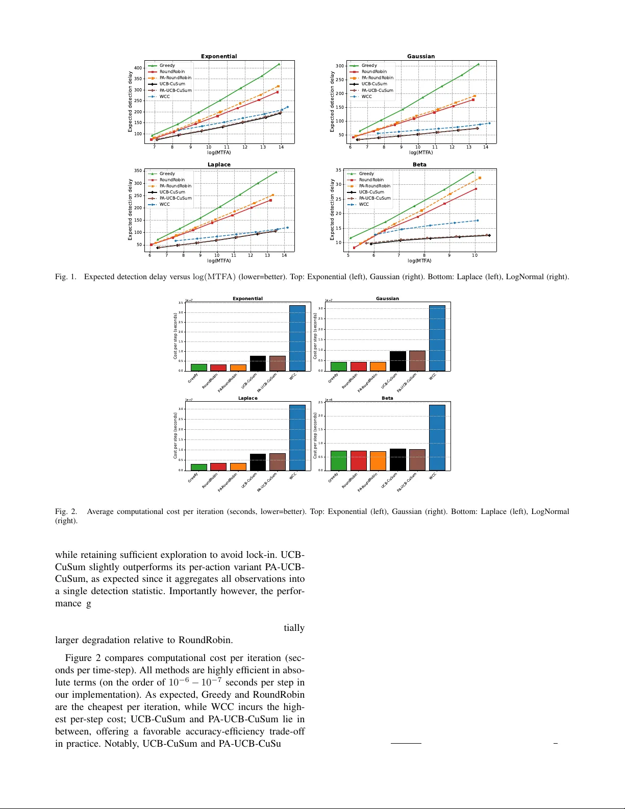
Learning Wher e to Look: UCB-Driven Controlled Sensing f or Quickest Change Detection Y u-Han Huang, Argyrios Gerogiannis, Subhonmesh Bose, V enugopal V . V eerav alli Abstract — W e study the multichannel quickest change de- tection problem with bandit feedback and controlled sensing, in which an agent sequentially selects one of the data streams to observe at each time-step and aims to detect an unknown change as quickly as possible while contr olling false alarms. Assuming known pre- and post-change distrib utions and al- lowing an arbitrary subset of streams to be affected by the change, we propose two novel and computationally efficient detection procedur es inspired by the Upper Confidence Bound (UCB) multi-armed bandit algorithm. Our methods adaptively concentrate sensing on the most informativ e str eams while pre- serving false-alarm guarantees. W e show that both procedures achieve first-order asymptotic optimality in detection delay under standard false-alarm constraints. W e also extend the UCB-driven contr olled sensing approach to the setting where the pre- and post-change distributions are unknown, except for a mean-shift in at least one of the channels at the change- point. This setting is particularly rele vant to the problem of learning in piecewise stationary en vironments. Finally , extensive simulations on synthetic benchmarks show that our methods consistently outperform existing state-of-the-art approaches while offering substantial computational savings. I . I N T R O D U C T I O N The problem of Quickest Change Detection (QCD) has an extensi ve range of applications in science and engineering, including quality control [1], earthquake detection [2], and online learning [3]. In this problem, an agent sequentially observes the environment through noisy samples, whose distribution shifts when the en vironment under goes a change. The goal for the agent is to detect the change as soon as possible while not triggering false alarms too often. See [4], [5], [6], [7] for books and survey articles on this topic. In this work, we study a variant of QCD, referred to as multichannel bandit QCD [8], [9], [10], which is a special case of the more general problem of QCD with controlled sensing that was introduced in [11] and further studied in [12]. In the multichannel bandit QCD problem, there are a finite number of data streams, and each data stream undergoes a different degree of shift in its distribution when the change occurs. The agent can only sample from one stream at a time, and therefore requires a carefully designed control polic y that selects which data stream to observe. In particular , the change detector and the control policy have to be designed jointly to achiev e the best tradeoff between detection delay and false alarm rate. A canonical example application of the QCD problem with controlled sensing, described in [11], is the surveillance system with a limited number of sensors that can be steered in different directions and locations. In this scenario, only a few sensors with specific positions can detect the change, as changes are localized in certain areas. Our motiv ation for studying the multichannel bandit QCD problem comes from detection-augmented learning in piece- wise stationary en vironments [13], [14], where one detects changes in the en vironment to restart stationary learning algorithms. T o detect such changes, one cannot rely on the optimal learned algorithm over a stationary interv al to detect changes in the environment quickly; it requires forced exploration. In this context, each channel corresponds to an action chosen for forced exploration, with the observations being the rew ards obtained from that action. When the learning environment changes, this change is reflected in the rew ard distributions obtained from the exploration actions, but the degree to which the distribution changes can vary across different actions. Current strategies for change detec- tion typically cycle through the various exploration actions in a round-robin fashion [15], [13], [14]. The round-robin approach is w asteful if only a small subset of the actions see significant shifts in distribution. Ideally , one would like to only explore actions for which the distribution shift is the most pronounced, making it a multichannel bandit QCD problem instance. A greedy algorithm for the multichannel bandit QCD prob- lem was proposed in [8] that samples a single channel until a cumulativ e log-likelihood ratio statistic for that channel exceeds a certain positi ve threshold or falls belo w zero. In the former case, a change is declared, and in the latter , the algo- rithm discards the observ ations from the channel, and repeats the process on the next channel. This greedy algorithm was shown to possess certain asymptotic optimality properties in terms of the tradeoff between delay delay and the false alarm rate when only a single channel is af fected by the change or all af fected channels see identical distribution shifts. This algorithm can be far from optimal when there is more than one affected channel and the distribution shifts can v ary significantly across actions. Intuiti vely , the greedy algorithm can focus on a single channel with a small distribution shift and declare a change with a large delay , never getting to sample another channel with a larger distribution shift, capable of certifying the change with far fewer samples. T o circumvent this challenge, the authors of [11] proposed the ϵ - Greedy Change Detector ( ϵ -GCD) for the general problem of QCD with controlled sensing. This algorithm, ho wever , is not (asymptotically) optimal; the worst-case delay can increase with the pre-change duration, as pointed out by [12]. An asymptotically optimal procedure for the general prob- lem of QCD with controlled sensing, called the W indowed- Chernoff-Cumulati ve Sum (WCC) procedure, was provided in [12]. In the special case of the multichannel bandit QCD problem, the WCC procedure chooses which channel to sample based on a windo wed maximum-likelihood estimate (MLE) of the set of channels that are af fected by the channel, and then chooses the channel with the lar gest potential distribution shift within that set. In addition, to avoid being unduly biased by the MLE, the WCC procedures performs random exploration of the other channels at o ( n ) time-steps ov er a time-horizon of length n . The observations from the chosen channels at each time-step are then fed into a windowed Cumulati ve Sum (CuSum) test for detecting the change. While the WCC procedure is asymptotically optimal for the multichannel bandit QCD problem, the control policy , which is designed to work for the general problem of QCD with controlled sensing, is not well-matched to the multi- channel special case. In particular , the number of subsets over which the MLE is computed grows exponentially with the number of channels. Another aspect of the WCC procedure that might make it less useful in the multichannel setting is that the observations across channels are combined into a single windo wed CuSum test for change detection. As discussed in Section V, this aspect does not allow the WCC procedure to be easily generalized to the setting where the pre- and post-change distrib utions of the observ ations from the channels are unknown. Giv en the similarity between the multi-armed bandit (MAB) and the multichannel bandit QCD problems, it is nat- ural to ask if one can dev elop MAB-like control policies for the latter problem. In order to do so, we need to identify an appropriate (pseudo) reward that can be used to guide action selection for change detection. Since the channel with the largest distrib ution shift (measured in terms of the Kullback- Leibler (KL) di vergence) will generate observ ations that hav e the largest av erage log-likelihood ratio (LLR) after the change, we may use LLR of the observations as the rew ard. W e design efficient procedures for the multichannel bandit QCD problem by combining the popular Upper Confidence Bound (UCB) MAB algorithm with CuSum change detection by viewing LLRs as re wards from the actions. Concretely , our contributions are as follows: (i) W e pro- pose UCB-CuSum , a bandit QCD procedure using UCB- based action selection to compute a CuSum statistic for change detection that is proven to be asymptotically optimal. (ii) W e generalize the above algorithm to P A-UCB-CuSum that maintains a separate CuSum statistic for each action for change detection, which is sho wn to offer a straightforward extension to settings with unkno wn pre- and post-change distributions. (iii) The proposed methods are empirically shown to outperform prior methods. I I . P R O B L E M F O R M U L A T I O N In this section, we formally define a multichannel bandit QCD problem. W e start by defining some no- tations. Let [ n ] : = { 1 , . . . , n } for any n ∈ N , and { X a,n : a ∈ [ K ] , n ∈ N } be K sequences of mutually inde- pendent stochastic observations indexed by the action a and the time-step n . For each action a , there are two densities the observation X a,n can possibly follo w: the pre-change density f a, 0 and the post-change density f a, 1 . At some time-step ν , referred to as the chang e-point , the underlying distributions of the stochastic observ ations could possibly change, i.e., for a ∈ [ K ] and n ∈ N , X a,n ∼ ( f a, 1 , n ≥ ν and a ∈ A , f a, 0 , otherwise , (1) where A ⊆ [ K ] is an nonempty subset that denotes the actions that undergo a distrib utional shift in the observations. In other words, for action a in the subset A , the observations follows the pre-change density f a, 0 before the change-point ν and follows the post-change density f a, 1 after the change- point ν . For actions that are not in the subset A , the observations follows f a, 0 before and after ν , as the change does not af fect the stochastic properties associated with these actions. The densities f a, 0 and f a, 1 are with respect to the same dominating measure λ , and they are all fully kno wn by the agent. 1 Howe ver , the change-point ν and the subset A are deterministic and completely unknown to the agent. W e also make the following assumptions, which does not impose a strict restriction on the pre- and post-change densities. Assumption 1: Assume that the KL Diver gence between f a, 1 and f a, 0 is positiv e, i.e., for an y a ∈ [ K ] , D ( f a, 1 || f a, 0 ) : = Z log ( f a, 1 /f a, 0 ) f a, 1 dλ > 0 . (2) In addition, assume that there exists a constant v < ∞ such that for any a ∈ [ K ] , log ( f a, 1 /f a, 0 ) is v -sub-Gaussian, i.e., for any θ ∈ R , log  Z exp ( θ (log ( f a, 1 /f a, 0 ) − D ( f a, 1 || f a, 0 ))) f a, 1 dλ  ≤ v 2 θ 2 . (3) At time-step n , the agent chooses an action A n to deter- mine which data stream to observe. These actions are deter- mined based on past observations; in particular , A n is F n − 1 measurable where F n − 1 : = σ  X A 1 , 1 , . . . , X A n − 1 ,n − 1  is the filtration generated by all observations collected prior to time-step n . The sequence of actions A : = { A n : n ∈ N } forms a contr ol policy . Based on the noisy observ ations obtained from the control policy , the agent decides whether a change has occurred or not. The stopping time at which the agent detects a change is denoted by T , and we refer to the pair ( A, T ) as the bandit QCD pr ocedur e , as these two components determine the detection delay and the false alarm frequency . W e use P A ν, A and E A ν, A to denote the measure and expec- tation when the agent uses A as its control policy , and the density associated with actions in A changes at ν . W e also use P A ∞ and E A ∞ to denote those when the agent uses A as its control policy and no changes occur . F or the false alarm and detection delay metrics, we employ Lorden’ s criterion [16]. The false alarm is ev aluated by the mean time to false 1 In our experiments, we explore cases where the pre- and post-change densities are bounded but not known. alarm E A ∞ [ T ] , 2 and the detection delay is ev aluated by the worst-case, ov er all possible change-points and pre-change observations, expected detection delay conditioned on the filtration F ν − 1 , i.e., for any control policy A and A ⊆ [ K ] , J A ( A, T ) : = sup ν ∈ N ess sup E A ν, A h ( T − ν + 1) +    F ν − 1 i (4) where ( x ) + : = max { x, 0 } is the positive part of x ∈ R . The definition in (4) follows from the delay measure in [12]. The goal of the agent is to minimize the worst-case expected delay J A A , while controlling the mean time to false alarm to be above a predetermined level γ , i.e., min T ,A J A ( A, T ) , subject to E A ∞ [ T ] ≥ γ . (5) I I I . O U R P RO C E D U R E S A. UCB-CuSum Procedur e In the QCD problem under Lorden’ s criterion without control sensing, i.e., K = 1 and A = { 1 } , the CuSum test [17] is asymptotically optimal as γ → ∞ [16], [18]. The CuSum statistic is computed by a recursion that adds the LLR of the observation at time-step n with the positiv e part of the CuSum statistic at the pre vious time-step n − 1 . The CuSum test raises an alarm whenev er the CuSum statistic surpasses a constant threshold. Due to the asymptotic optimality , it is natural to expect that a procedure that utilizes a CuSum-like statistic will perform well in the bandit QCD problem. Thus, following the recursion along the lines of [9], [12], we define a CuSum-like statistic: for n ∈ N , C A n : =  C A n − 1  + + LLR ( A n , X A n ,n ) (6) with C A 0 : = 0 and the LLR function LLR ( a, x ) : = log ( f a, 1 ( x ) /f a, 0 ( x )) . (7) The procedure using the CuSum-like statistic in (6) stops whenev er the statistic surpasses a constant threshold b , i.e., T A b : = inf  n ∈ N : C A n ≥ b  . (8) W e choose b to satisfy the false alarm constraint in (5). T o achieve faster detection, the control policy A should select the action with the largest a verage LLR after the change-point, so that the CuSum-like statistic in (6) grows quickly to surpass the threshold. Therefore, to learn the optimal action that leads to the lar gest increment in the statistic in (6), we employ an upper confidence bound (UCB) algorithm [19] with periodic restarts A UCB as our control policy A . First, we partition the entire horizon into intervals of length W , i.e., N = ∪ ∞ j =1 I j with the j th interval I j : = { ( j − 1) W + 1 , . . . , j W } . In each interv al, we apply the UCB algorithm to select the action and restart the control policy at the start of the next interval. Notice that we restart our UCB algorithm every W time-steps. W ithout such a restart, the control policy tends to heavily concentrate on the action with the lar gest a verage LLR before the change. 2 This false alarm metric is different from but related to the false alarm probability used in many prior works. Consequently , the control policy rarely explore other actions, leading to delayed detection after the change. W e vie w the LLR of the observation X A n ,n from action A n as the reward at time-step n , that is, R n : = LLR ( A n , X A n ,n ) . (9) Let j = ⌈ n/W ⌉ denote the index of the current interval, and let m = ( j − 1) W + 1 denote the start of the current interval. In addition, we use N a,n to denote the times action a is selected since the start of the current interv al, i.e., N a,n : = n X i = m I { A i = a } . (10) Let ˆ µ a,n denote the empirical mean of the re wards from action a since the start of the current interval, i.e., ˆ µ a,n : =      1 N a,n n X i = m R i I { A i = a } , N a,n > 0 0 , N a,n = 0 . (11) Then, the UCB index is defined as follo ws: UCB ( a, n ) : = ˆ µ a,n + s 4 v log W N a,n , (12) and the UCB algorithm selects the action with the largest UCB index, i.e., A UCB : = { A n : n ∈ N } with A n : = argmax a ∈ [ K ] UCB ( a, n ) . (13) Combining the UCB control policy A UCB in (13) with the stopping time T A b in (8), we propose the UCB-CuSum Pro- cedure  A UCB , T A UCB b  , which is illustrated in Algorithm 1. This procedure uses the CuSum-like statistic in (6) that combines LLRs from all actions together . Algorithm 1 UCB-CuSum Procedure Input: Threshold b , Interval length W Initialize C ← 0 and n ← 0 . repeat if n mo d W = 0 then Set N a ← 0 , ˆ µ a ← 0 , UCB a ← ∞ for a ∈ [ K ] . end if Choose action A ∈ argmax a ∈ [ K ] UCB a . Receiv e observation X . Update statistic C ← max { C , 0 } + LLR ( A, X ) . Compute rew ard R ← LLR ( A, X ) . Update mean reward ˆ µ A ← ( N a µ + R ) / ( N a + 1) . Update index UCB A ← ˆ µ A + p 4 v log W / N A . Update number of pulls N A ← N A + 1 . n ← n + 1 . until C ≥ b In the following result, we characterize the performance of the UCB-CuSum procedure. Theor em 1 (Asymptotic optimality of UCB-CuSum): W ith b = log γ , E A UCB ∞ h T A UCB b i ≥ γ . As γ , W → ∞ with W = o (log γ ) , we have J A  A UCB , T A UCB b  ≤ log γ I A (1 + o (1)) . (14) where I A : = max a ∈A D ( f a, 1 || f a, 0 ) . The formal proof is included in Appendix . Here, we provide a sketch. The lo wer bound on the mean time to false alarm follows from Lemma 1 in [12], which relies on the martingale property of a Shiryaev-Roberts (SR)-like statistic and the optional sampling theorem. T o prove the upper bound on the expected delay , we establish that J A  A UCB , T A UCB b  ≤ W + E A UCB 1 , A h T A UCB b i , (15) where recall that E A UCB 1 , A denotes the expectation when the change occurs at time-step 1 . The intuition behind this step is that the duration between the change-point ν and the subsequent restart ℓ is at most W , and that E A UCB ν, A [ T A UCB b − ℓ + 1 |F ν − 1 ] is roughly equal to E A UCB 1 , A [ T A UCB b ] , as the obser- vations after the restart ℓ under P A UCB ν, A and all observ ations under P A UCB 1 , A follow the same post-change distribution. Next, we upper bound E A UCB 1 , A [ T A UCB b ] . While our precise argument relies on Proposition 1 in [12], we provide some intuition here. T o do so, consider the notation, Y A UCB i : = iW X j =( i − 1) W +1 LLR  A j , X A j ,j  , i ∈ N . (16) Thus, Y i is the sum of the LLR ov er the i -th W -step window . Let ¯ C A UCB iW := P iW j =1 Y A UCB j accumulate these Y A UCB j ’ s across windows up to the i -th one. W ith this notation, notice that T A UCB b ≤ W inf n i ∈ N : ¯ C A UCB iW ≥ b o (17) T o obtain the expected hitting time of ¯ C A UCB iW ’ s, we view the LLR’ s as re wards for an UCB algorithm in (13) for which the expectation of Y A UCB i , gi ven the history F ( i − 1) W , precisely equals the maximum possible cumulative reward W I A less the regret of the UCB algorithm. W e borrow an upper bound on that regret from Theorem 7.1 in [20]. In turn, this step provides a minimum expected positive drift on Y A UCB i ’ s using regret analysis of the UCB algorithm, with which we apply the level crossing result in Proposition 1 for ¯ C A UCB iW from [12]. Putting it together, we obtain E A UCB 1 , A h T A UCB b i ≤ W  b + c  1 + √ b  W I A − P a :∆ a > 0  3∆ a + 16 log W ∆ a  . The rest follows from taking γ → ∞ with W = o (log γ ) . UCB-CuSum is in fact asymptotically optimal in the regime γ → ∞ ; optimality follo ws from a kno wn lo wer bound on the worst-case expected delay J A of any multi- channel bandit QCD procedure that satisfies the false alarm constraint. More precisely , as γ → ∞ , inf ( A,T ): E A ∞ [ T ] ≥ γ J A ( A, T ) ≥ log γ I A (1 + o (1)) , (18) according to Theorem 1 in [12]. B. P er-Action-UCB-CuSum Pr ocedure The CuSum-like statistic in (6) accumulates LLRs asso- ciated with different pairs of pre- and post-change distribu- tions. This is different from the original CuSum statistic, which only in volves a single pair of pre- and post-change distributions. Now , we study an alternate CuSum statistic that is defined by the follo wing recursion: for any a ∈ [ K ] and n ∈ N , C A a,n : = (  C A a,n − 1  + + LLR ( a, X a,n ) , A n = a C A a,n − 1 , otherwise (19) with C A a, 0 : = 0 and LLR defined in (7). The change detection procedure using the statistic in (19) flags a change whenev er one of these statistics surpasses a constant threshold b , i.e., ˜ T A b : = inf  n ∈ N : C A a,n ≥ b for some a ∈ [ K ]  . (20) Combining with the UCB algorithm, we propose the Per-Action (P A)-UCB-CuSum procedure  A UCB , ˜ T A UCB b  , which computes a CuSum statistic in (19) for each action separately . The P A-UCB-CuSum procedure is illustrated in Algorithm 2. This algorithm is motiv ated by the fact that it generalizes better to the case when the pre- and post- change distributions are not known, and the statistics must be computed using generalized LLRs, as we illustrate later in Section V. Algorithm 2 P A-UCB-CuSum Procedure Input: Threshold b , Interval length W Initialize n ← 0 and C a ← 0 for all a ∈ [ K ] . repeat if n mo d W = 0 then Set N a ← 0 , ˆ µ a ← 0 , UCB a ← ∞ for a ∈ [ K ] . end if Choose action A ∈ argmax a ∈ [ K ] UCB a . Receiv e observation X . Update statistic C A ← max { C A , 0 } + LLR ( A, X ) . Compute rew ard R ← LLR ( A, X ) . Update mean reward ˆ µ A ← ( N a µ + R ) / ( N a + 1) . Update index UCB A ← ˆ µ A + p 4 v log W / N A . Update number of pulls N A ← N A + 1 . n ← n + 1 . until C a ≥ b for some a ∈ [ K ] Our ne xt result resonates the same message as in Theorem 1 for the P A-UCB-CuSum procedure, claiming its asymptotic optimality under the false alarm constraint in (5). Theor em 2 (Asymptotic optimality of P A-UCB-CuSum): W ith b = log γ , E A UCB ∞ h ˜ T A UCB b i ≥ γ and as γ , W → ∞ with W = o (log γ ) , we ha ve J A  A UCB , ˜ T A UCB b  ≤ log γ I A (1 + o (1)) . (21) The proof of the upper bound on the worst-case expected delay J A ( A UCB , ˜ T A UCB b ) follows similar steps as in the proof of Theorem 1. Ho wever , we cannot apply Lemma 1 in [12] to ar gue the lo wer bound on the false alarm constraint. Instead, we construct an SR-like statistic for each arm separately , and then show that the difference between the time-step and the sum of all SR-like statistics forms a martingale. Then, the rest of the steps follow the same line in Lemma 1 in [12]. The formal proof is included in Appendix . Again, Theorem 1 in [12] certifies the asymptotic opti- mality of the P A-UCB-CuSum procedure. In other words, asymptotically speaking ( γ → ∞ ), the per-action and the accumulated UCB-based CuSUM procedures have similar performance. W e study their dif ferences empirically , and specifically in the case where the distributions are unknown with generalized LLRs, in the ne xt section. I V . E X P E R I M E NTA L S T U DY In this section, we numerically e v aluate how UCB-CuSum and the P A-UCB-CuSum algorithms on the multichannel bandit QCD problem using synthetic data. W e further com- pare their performance against the leading approaches from prior works. A. Algorithmic Benchmarks W e compare against four baselines. First, we include WCC [12], the state-of-the-art procedure that is first-order optimal and empirically strong. Second, we consider the Gr eedy procedure (as in [10]), which samples a single component while maintaining a CuSum statistic: it repeatedly pulls the current component until its cumulative LLR either crosses the detection threshold (in which case it declares an alarm) or resets to zero (in which case it discards past samples and switches to the next component). This method is known to enjoy asymptotic optimality guarantees in special cases, e.g., when only one component is affected or when all affected components share the same post-change distribution [8], [21]. Finally , as an additional benchmark, we include RoundRobin . This algorithm cyclically samples all components and aggregates the resulting LLRs into a single global statistic, declaring an alarm once this statistic exceeds its threshold. T o make a comparison with the per- action variant of UCB-CuSum, we also include a per-action RoundRobin (P A-RoundRobin) which maintains a unique statistic for each action. Greedy and RoundRobin algorithms offer no optimality guarantees. B. Experimental Setup W e consider a bandit QCD problem with K = 10 inde- pendent action-channels, where selecting action a ∈ [ K ] at time n yields an observ ation X a,n . W e consider four dif ferent observation distributions: (i) Gaussian, (ii) Exponential, (iii) Laplace, and (i v) Beta, where only the last distrib ution family yields bounded observ ations in [0 , 1] . In the pre-change regime ( n < ν ), the observations are i.i.d. across time with X a,n ∼ N (0 , 1) in the Gaussian case, X a,n ∼ Exp(1) (mean 1 ) in the Exponential case, X a,n ∼ Laplace(0 , 1) in the Laplace case, and for Beta, X a,n ∼ Beta( α , β ) with and mean equal to 0 . 01 , where throughout we set α + β = 2 . At the change-point ν , for all cases except Beta (since it is bounded in [0 , 1] ) a sparse subset of the channels becomes anomalous according to the shift v ector ξ = [0 , 0 , 0 . 1 , 0 , 0 , 0 . 1 , 0 , 0 , 1 , 0] ⊤ . and the shift is added to the corresponding actions. W ith the Beta distributed observ ations, we replace 0 . 1 with 0 . 04 and 1 with 0 . 19 . This design is intentionally sparse and heter ogeneous : multiple components change, yet the mag- nitudes are unequal (two mild changes at le vel 0 . 1 and one strong change at level 1 ). As a result, greedy selection rules can be brittle: once the Greedy policy locks onto a mildly-changed channel, it may continue sampling it and accumulate evidence too slowly , thereby delaying discovery of the strongly-changed channel. This behavior is consistent with the f act that Greedy does not generally admit asymptotic optimality guarantees in such heterogeneous sparse settings, ev en though it can perform well empirically in simpler regimes [12]. Notice that RoundRobin continues to probe all channels, preventing permanent lock-in; in our setting, the presence of a suf ficiently strong change ( ξ 9 = 1 ) suggests that periodic exploration can yield informativ e post-change samples and enables better detection compared to Greedy . C. Experimental P arameters and Metrics W e follow the parameter choices recommended in the original works, setting w = ⌈ 5 log b ⌉ and q = ⌈ log w ⌉ for WCC. As per our theory , we set W = ⌈ 8 log b ⌉ for Bandit- CuSum and P A-Bandit-CuSum. Greedy and RoundRobin do not hav e associated parameter choices. Performance is ev aluated via Monte-Carlo simulation in terms of (i) mean time to false alarm (MTF A) and (ii) expected detection delay , a veraging over 200 K independent trials. T o generate MTF A–delay curves, we sweep the detec- tion threshold to obtain dif ferent operating points; in practice, this can be done by selecting target MTF A levels γ and setting b = log γ . In all figures, we report expected detection delay versus log(MTF A) . In addition to statistical perfor- mance, we also report computational efficienc y , quantified as the a verage cost per step (wall-clock time per algorithm iteration), av eraged over simulation runs. D. Experimental Results Figure 1 reports the trade-of f between expected detection delay and log (MTF A) . Across the dif ferent observ ation models, UCB-CuSum and P A-UCB-CuSum attain the best performance, achie ving the smallest delay for a gi ven MTF A lev el, consistently improving over WCC and substantially outperforming the Greedy and RoundRobin baselines. This behavior is consistent with heterogeneous sparse-change de- sign: Greedy can lock onto mildly-changed channels and thus accumulates evidence slowly , while RoundRobin allocates a fixed fraction of samples to unaffected channels (which improv es over Greedy), leading to lar ger delay . In contrast, UCB-CuSum adapti vely concentrates sam- pling on informative channels with the largest changes, 7 8 9 10 11 12 13 14 log(MTF A) 100 150 200 250 300 350 400 Expected detection delay Exponential Gr eedy R oundR obin P A -R oundR obin UCB-CuSum P A -UCB-CuSum WCC 6 7 8 9 10 11 12 13 14 log(MTF A) 50 100 150 200 250 300 Expected detection delay Gaussian Gr eedy R oundR obin P A -R oundR obin UCB-CuSum P A -UCB-CuSum WCC 6 7 8 9 10 11 12 13 14 log(MTF A) 50 100 150 200 250 300 350 Expected detection delay Laplace Gr eedy R oundR obin P A -R oundR obin UCB-CuSum P A -UCB-CuSum WCC 5 6 7 8 9 10 log(MTF A) 10 15 20 25 30 35 Expected detection delay Beta Gr eedy R oundR obin P A -R oundR obin UCB-CuSum P A -UCB-CuSum WCC Fig. 1. Expected detection delay versus log(MTF A) (lower=better). T op: Exponential (left), Gaussian (right). Bottom: Laplace (left), LogNormal (right). Gr eedy R oundR obin P A -R oundR obin UCB-CuSum P A -UCB-CuSum WCC 0.0 0.5 1.0 1.5 2.0 2.5 3.0 3.5 Cost per step (seconds) 1e 7 Exponential Gr eedy R oundR obin P A -R oundR obin UCB-CuSum P A -UCB-CuSum WCC 0.0 0.5 1.0 1.5 2.0 2.5 3.0 Cost per step (seconds) 1e 7 Gaussian Gr eedy R oundR obin P A -R oundR obin UCB-CuSum P A -UCB-CuSum WCC 0.0 0.5 1.0 1.5 2.0 2.5 3.0 Cost per step (seconds) 1e 7 Laplace Gr eedy R oundR obin P A -R oundR obin UCB-CuSum P A -UCB-CuSum WCC 0.0 0.5 1.0 1.5 2.0 2.5 Cost per step (seconds) 1e 6 Beta Fig. 2. A verage computational cost per iteration (seconds, lower=better). T op: Exponential (left), Gaussian (right). Bottom: Laplace (left), LogNormal (right). while retaining sufficient exploration to av oid lock-in. UCB- CuSum slightly outperforms its per-action variant P A-UCB- CuSum, as expected since it aggregates all observations into a single detection statistic. Importantly howe ver , the perfor- mance gap between UCB-CuSum and P A-UCB-CuSum is small, indicating strong robustness to per -action decompo- sition. In contrast, P A-RoundRobin exhibits a substantially larger degradation relativ e to RoundRobin. Figure 2 compares computational cost per iteration (sec- onds per time-step). All methods are highly efficient in abso- lute terms (on the order of 10 − 6 − 10 − 7 seconds per step in our implementation). As expected, Greedy and RoundRobin are the cheapest per iteration, while WCC incurs the high- est per-step cost; UCB-CuSum and P A-UCB-CuSum lie in between, offering a fav orable accuracy-ef ficiency trade-off in practice. Notably , UCB-CuSum and P A-UCB-CuSum are markedly more ef ficient than WCC, achieving substantially lower per-step runtime while also attaining better statistical performance. V . T O W A R D S U N K N OW N D I S T R I B U T I O N S The procedures above rely on the knowledge of the dis- tributions ( f a, 0 , f a, 1 ) to compute LLR( a, x ) and the CuSum statistics. In a variety of applications, such distributions are not kno wn. As a first step toward that scenario, we replace LLR by a per-action generalized likelihood ratio (GLR) statistic and retain the same UCB-dri ven controlled sensing template for QCD. Specifically , we use the Bernoulli GLR statistic of [15]: giv en observations X 1 , . . . , X n ∈ [0 , 1] , define ˆ µ t 1 : t 2 := 1 t 2 − t 1 +1 P t 2 t = t 1 X t and kl( p, q ) := p ln p q + (1 − p ) ln 1 − p 1 − q . Then the GLR statistic GLR( n ) is max 1 ≤ s 0 that does not depend on b, I A , and W , E A UCB 1 , A h T A UCB b i ≤ W  b + c  1 + √ b  W I A − P a :∆ a > 0  3∆ a + 16 log W ∆ a  (28) where ∆ a = I A − D ( f a, 1 || f a, 0 ) . Pr oof: For any n ∈ N , define the statistic ¯ C A UCB n to be the sum of the LLRs up to time-step n , i.e., ¯ C A UCB n : = n X i =1 LLR ( A i , X A i ,i ) . (29) Also, we define ¯ T A UCB b to be the stopping time at which ¯ C A UCB n crosses the threshold b at the end of an W -length interval I i = { ( i − 1) W + 1 , . . . , iW } , i.e., ¯ L A UCB b : = inf n i ∈ N : ¯ C A UCB iW ≥ b o and ¯ T A UCB b : = ¯ L A UCB b W . (30) Since ¯ C A UCB n ≤ C A UCB n for all n ∈ N , ¯ T A UCB b ≥ T A UCB b . Now , for any i ∈ N , define the filtration G i : = σ ( X 1 , . . . , X iW ) and the following statistic to be the dif ference of ¯ C A UCB n ov er interval I i = { ( i − 1) W + 1 , . . . , iW } , i.e., Y A UCB i : = ¯ C A UCB iW − ¯ C A UCB ( i − 1) W = iW X j =( i − 1) W +1 LLR  A j , X A j ,j  . (31) Recall that I A : = max a ∈A D ( f a, 1 || f a, 0 ) . Then, E A UCB 1 , A h Y A UCB i    G i − 1 i ( a ) = E A UCB 1 , A h Y A UCB i i = E A UCB 1 , A   iW X j =( i − 1) W +1 LLR  A j , X A j ,j    ( b ) ≤ W I A , (32) and E A UCB 1 , A h Y A UCB i |G i − 1 i = E A UCB 1 , A   iW X j =( i − 1) W +1 LLR  A j , X A j ,j    ( c ) ≥ W I A − X a :∆ a > 0  3∆ a + 16 log W ∆ a  . (33) In step ( a ) , we leverage the fact that Y A UCB i is independent of G i − 1 . In step ( b ) , we apply the fact that E A UCB 1 , A  LLR  A j , X A j ,j  ≤ I A . In step ( c ) , we apply the regret upper bound in Theorem 7.1 in [20], as the LLRs are the rew ards of the UCB algorithm. Recall that we assume R (log ( f a, 1 /f a, 0 ) − D ( f a, 1 || f a, 0 )) 2 f a, 1 dλ = v < ∞ for any a ∈ [ K ] . Then, E A UCB 1 , A   Y A UCB i  2     G i − 1  ( a ) = E A UCB 1 , A   Y A UCB i  2  = E A UCB 1 , A   iW X j =( i − 1) W +1 iW X k =( i − 1) W +1 LLR  A j , X A j ,j  LLR ( A k , X A k ,k )   = iW X j =( i − 1) W +1 iW X k =( i − 1) W +1 E A UCB 1 , A  LLR  A j , X A j ,j  LLR ( A k , X A k ,k )  = iW X j =( i − 1) W +1 E A UCB 1 , A h  LLR  A j , X A j ,j  2 i + 2 iW X j =( i − 1) W +1 iW X k = j +1 E A UCB 1 , A  LLR  A j , X A j ,j  LLR ( A k , X A k ,k )  ( b ) ≤ W v + W 2 I 2 A (34) where step ( a ) stems from the fact that Y A UCB i is independent of G i − 1 , and step ( b ) follows from Assumption 1. Then, we can apply Proposition 1 in [12] and obtain that E A UCB 1 , A h ¯ L A UCB b i ≤ b + c  1 + √ b  W I A − P a :∆ a > 0  3∆ a + 16 log W ∆ a  . (35) Thus, E A UCB 1 , A h T A UCB b i ( a ) ≤ E A UCB 1 , A h ¯ T A UCB b i ( b ) ≤ W  b + c  1 + √ b  W I A − P a :∆ a > 0  3∆ a + 16 log W ∆ a  (36) where step ( a ) follows from the fact that ¯ T A UCB b ≥ T A UCB b , and step ( b ) results from (35). W ith Lemma 2, we deri ve J A  A UCB , T A UCB b  ≤ W + W  b + c  1 + √ b  W I A − P a :∆ a > 0  3∆ a + 16 log W ∆ a  . (37) Then, as W, b → ∞ with W = o ( b ) , J A  A UCB , T A UCB b  ≤ b I A (1 + o (1)) . (38) This completes the proof of Theorem 1. T o prove that E A UCB ∞ h ˜ T A UCB log γ i ≥ γ , we first construct the following SR-like statistic [22] for each action: for a ∈ [ K ] and n ∈ N , S A UCB a,n : =     S A UCB a,n − 1 + 1  exp (LLR ( a, X a,n )) , A n = a S A UCB a,n − 1 , otherwise (39) with S a, 0 : = 0 . In addition, we define the following statistic as the sum of the SR-like statistic in (39): for each n ∈ N , S n : = X a ∈ [ K ] S a,n . (40) Thereupon, we can see that { S n : n ∈ N } is adapted to the filtration {F n : n ∈ N } . W e show that { S n − n : n ∈ N } is a martingale with respect to the filtration {F n : n ∈ N } under E A UCB ∞ : for any n ∈ N , E A UCB ∞ [ S n − n |F n − 1 ] = E A UCB ∞   S A n ,n + X a  = A n S a,n − n      F n − 1   = E A UCB ∞   ( S A n ,n − 1 + 1) exp  LLR  A n , X A n ,M A n ,n  + X a  = A n S a,n − 1 − n      F n − 1   = ( S A n ,n − 1 + 1) E A UCB ∞  exp  LLR  A n , X A n ,M A n ,n    F n − 1  + X a  = A n S a,n − 1 − n = ( S A n ,n − 1 + 1) E A UCB ∞  f A n , 1 ( X A n ,n ) /f A n , 0 ( X A n ,n )   F n − 1  + X a  = A n S a,n − 1 − n = X a ∈ [ K ] S a,n − 1 − ( n − 1) = S n − 1 − ( n − 1) . (41) W e can see that S n ≥ S a,n ≥ exp ( C a,n ) for any a ∈ [ K ] and n ∈ N . Therefore, E A UCB ∞ h ˜ T A UCB log γ i ( a ) = E A UCB ∞ h S ˜ T A UCB log γ i ≥ E A UCB ∞ h exp  C ˜ T A UCB log γ i ( b ) ≥ γ . (42) where step ( a ) follows from Optional Sampling Theorem, and step ( b ) stems from the definition of ˜ T A UCB log γ in (20). T o prove (21), we sho w that as W, b → ∞ with W = o ( b ) , J A  A UCB , ˜ T A UCB b  ≤ b I A (1 + o (1)) . (43) The proof of this upper bound on J A requires the following lemma similar to Lemma 1. Lemma 3: For any change-point ν ∈ N and A ⊆ [ K ] , E A UCB ν, A   ˜ T A UCB b − ν + 1  +    F ν − 1  ≤ W + E A UCB 1 , A h ˜ T A UCB b i . (44) Pr oof: Recall that ℓ : = argmin { i ∈ N : i ≥ ν and i mo d W = 1 } is the first time-step at which the UCB algorithm restarts after the change occurs. W e define the CuSum-like statistic that accumulates the LLRs starting from time-step ℓ using the following recursion: for n ≥ ℓ and a ∈ [ K ] , C A UCB a,ℓ : n : =    max n C A UCB a,ℓ : n − 1 , 0 o + LLR ( a, X a,n ) , A n = a C A UCB a,ℓ : n − 1 , otherwise (45) with C A UCB a,ℓ : ℓ − 1 : = 0 . W e also define a new stopping time that stops when C A UCB a,ℓ : n crosses the threshold b : ˜ T A UCB b,ℓ : = inf n n ≥ ℓ : C A UCB a,ℓ : n ≥ b for some a ∈ [ K ] o . (46) Then, following similar steps in (26), E A UCB ν, A   ˜ T A UCB b − ν + 1  +    F ν − 1  ( a ) ≤ E A UCB ν, A   ˜ T A UCB b,ℓ − ν + 1  +    F ν − 1  = E A UCB ν, A h ˜ T A UCB b,ℓ − ν + 1    F ν − 1 i = ℓ − ν + E A UCB ν, A h ˜ T A UCB b,ℓ − ℓ + 1    F ν − 1 i ( b ) ≤ W + E A UCB ν, A h ˜ T A UCB b,ℓ − ℓ + 1    F ν − 1 i ( c ) = W + E A UCB ν, A h ˜ T A UCB b,ℓ − ℓ + 1 i ( d ) = W + E A UCB ℓ, A h ˜ T A UCB b,ℓ − ℓ + 1 i ( e ) = W + E A UCB 1 , A h ˜ T A UCB b, 1 i ( f ) = W + E A UCB 1 , A h ˜ T A UCB b i . (47) In step ( a ) , ˜ T A UCB b,ℓ ≥ ˜ T A UCB b almost surely , since we can show that C A UCB a,ℓ : n ≤ C A UCB a,n for n ≥ ℓ by induction. In step ( b ) , since ℓ is the first restart time-step after the change, ℓ − ν ≤ W . In step ( c ) , because C A UCB a,ℓ : n is independent the observ ations before time-step ℓ , we can utilize the fact that ˜ T A UCB b,ℓ is independent of F ℓ − 1 and F ν − 1 ⊆ F ℓ − 1 . Step ( d ) follows from the fact that X a,n follows the post-change density f a, 1 for n ≥ ℓ and a ∈ A when the change occurs either at ν or at ℓ . Step ( e ) results from the fact that X a,n follows the post-change density f a, 1 for n ≥ ℓ and a ∈ A under P A UCB ℓ, A , and that X a,n follows the post-change density f a, 1 for n ≥ 1 and a ∈ A under P A UCB 1 , A . In step ( f ) , ˜ T A UCB b = ˜ T A UCB b, 1 by the definitions in (19) and (45). W ith Lemma 3, we can derive that J A  A UCB , ˜ T A UCB b  ≤ W + E A UCB 1 , A h ˜ T A UCB b i . (48) T o upper bound E A UCB 1 , A h ˜ T A UCB b i , we need the following lemma. Lemma 4: For some constant c > 0 that does not depend on b, I A , and W , E A UCB 1 , A h ˜ T A UCB b i ≤ W  b + c  1 + √ b  W I A − I A  P a :∆ a > 0 3 + 16 log W (∆ a ) 2  (49) where ∆ a = I A − D ( f a, 1 || f a, 0 ) . Pr oof: First, let a ∗ : = argmax a ∈ [ K ] D ( f a, 1 || f a, 0 ) and define the following statistic to be the summation of the LLRs at time-steps when the control polic y chooses action a : for any a ∈ [ K ] and n ∈ N , ¯ C A UCB a,n : = n X i =1 I { A i = a } LLR ( a, X a,i ) . (50) Also, define ¯ T A UCB a,b to be the stopping time at which ¯ C A UCB a,n crosses the threshold b at the end of an W -length interv al I i = { ( i − 1) W + 1 , . . . , iW } , i.e., for any a ∈ [ K ] and n ∈ N , ¯ L A UCB a,b : = inf n i ∈ N : ¯ C A UCB a,iW ≥ b o and ¯ T A UCB a,b : = ¯ L A UCB a,b W . (51) Since ¯ C A UCB a,n ≤ C A UCB a,n for all n ∈ N and a ∈ [ K ] , ¯ T a ∗ ,b ≥ ˜ T A UCB b . Recall that G i : = σ ( X 1 , . . . , X iW ) for any i ∈ N and define the statistic: for any i ∈ N and a ∈ [ K ] , Y A UCB a,i : = ¯ C A UCB a,iW − ¯ C A UCB a, ( i − 1) W = iW X j =( i − 1) W +1 I { A i = a } LLR ( a, X a,j ) . (52) Then, E A UCB 1 , A h Y A UCB a ∗ ,i    G i − 1 i ( a ) = E A UCB 1 , A h Y A UCB a ∗ ,i i = E A UCB 1 , A   iW X j =( i − 1) W +1 E A UCB 1 , A [ I { A i = a ∗ } LLR ( a ∗ , X a ∗ ,j ) |F j − 1 ]   = E A UCB 1 , A   iW X j =( i − 1) W +1 I { A i = a ∗ } E A UCB 1 , A [LLR ( a ∗ , X a ∗ ,j ) |F j − 1 ]   ( b ) = E A UCB 1 , A   iW X j =( i − 1) W +1 I { A i = a ∗ } E A UCB 1 , A [LLR ( a ∗ , X a ∗ ,j )]   ( c ) ≤ W I A , (53) and E A UCB 1 , A h Y A UCB a ∗ ,i |G i − 1 i = E A UCB 1 , A   iW X j =( i − 1) W +1 I { A i = a ∗ } E A UCB 1 , A [LLR ( a ∗ , X a ∗ ,j )]   ( d ) ≥ W I A − I A X a :∆ a > 0 3 + 16 log W (∆ a ) 2 ! . (54) In step ( a ) , we apply the fact that Y A UCB a ∗ ,i is independent of G i − 1 . Step ( b ) follows from the fact that X a ∗ ,j is independent of F j − 1 . In step ( c ) , we apply the fact that E A UCB 1 , A [LLR ( a ∗ , X a ∗ ,j )] = I A . In step ( d ) , we apply the regret upper bound in Theorem 7.1 in [20], as the LLRs are the rewards of the UCB algorithm. Recall that we assume R (log ( f a, 1 /f a, 0 )) 2 f a, 1 dλ < ∞ for any a ∈ [ K ] . Then, E A UCB 1 , A   Y A UCB a ∗ ,i  2     G i − 1  ( a ) = E A UCB 1 , A   Y A UCB a ∗ ,i  2  = E A UCB 1 , A   iW X j =( i − 1) W +1 iW X k =( i − 1) W +1 I { A j = a ∗ } I { A k = a ∗ } LLR ( a ∗ , X a ∗ ,j ) LLR ( a ∗ , X a ∗ ,k )   ≤ iW X j =( i − 1) W +1 iW X k =( i − 1) W +1 E A UCB 1 , A [LLR ( a ∗ , X a ∗ ,j ) LLR ( a ∗ , X a ∗ ,k )] = iW X j =( i − 1) W +1 E A UCB 1 , A h (LLR ( a ∗ , X a ∗ ,j )) 2 i + 2 iW X j =( i − 1) W +1 iW X k = j +1 E A UCB 1 , A [LLR ( a ∗ , X a ∗ ,j ) LLR ( a ∗ , X a ∗ ,k )] ( b ) ≤ W v + ( W − 1) W I 2 A (55) where step ( a ) stems from the fact that Y A UCB a ∗ ,i is independent of G i − 1 , and step ( b ) follows from Assumption 1. Then, we can apply Proposition 1 in [12] and obtain that E A UCB 1 , A h L A UCB a ∗ ,b i ≤ b + c  1 + √ b  W I A − I A P a :∆ a > 0  3 + 16 log W (∆ a ) 2  . (56) Thus, E A UCB 1 , A h ˜ T A UCB b i ( a ) ≤ E A UCB 1 , A h ¯ T A UCB a ∗ ,b i ( b ) ≤ W  b + c  1 + √ b  W I A − I A P a :∆ a > 0  3 + 16 log W (∆ a ) 2  (57) where step ( a ) follows from the fact that ¯ T A UCB a ∗ ,b ≥ ˜ T A UCB b , and step ( b ) results from (56). W ith Lemma 4, we deri ve J A  A UCB , ˜ T A UCB b  ≤ W + W  b + c  1 + √ b  W I A − I A P a :∆ a > 0  3 + 16 log W (∆ a ) 2  . (58) Then, as W, b → ∞ with W = o ( b ) , J A  A UCB , ˜ T A UCB b  ≤ b I A (1 + o (1)) . (59) This completes the proof of Theorem 2.