Rational solutions for algebraic solitons in the massive Thirring model

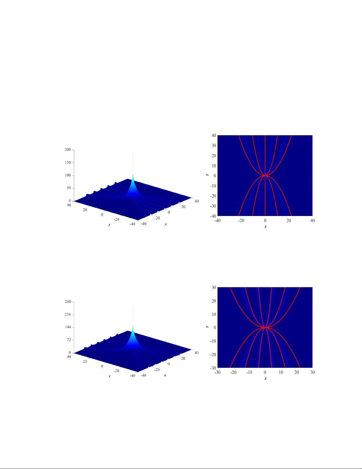
RA TIONAL SOLUTIONS F OR ALGEBRAIC SOLITONS IN THE MASSIVE THIRRING MODEL ZHEN ZHA O, CHENG HE, BAOFENG FENG, AND DMITR Y E. PELINOVSKY Abstract. An algebraic soliton of the massiv e Thirring mo del (MTM) is expressed b y the simplest rational solution of the MTM with the spatial decay of O ( x − 1 ). The corre- sp onding p oten tial is related to a simple em bedded eigen v alue in the Kaup–Newell spectral problem. This w ork fo cuses on the hierarch y of rational solutions of the MTM, in whic h the N -th mem b er of the hierarc hy describ es a nonlinear sup erposition of N algebraic solitons with iden tical masses and corresp onds to an em b edded eigenv alue of algebraic m ultiplicity N . W e sho w that the hierarc hy of rational solutions can be constructed b y using the double-W ronskian determinants. The nov elty of this work is a rigorous proof that eac h solution is deﬁned by a p olynomial of degree N 2 with 2 N arbitrary parame- ters, which admits N ( N − 1) 2 p oles in the upp er half-plane and N ( N +1) 2 p oles in the low er half-plane. Assuming that the leading-order polynomials ha ve exactly N real roots, we sho w that the N -th member of the hierarc hy describes the slo w scattering of N algebraic solitons on the time scale O ( √ t ). Corr esp onding author: Dmitry E. Pelinovsky; e-mail: p elino d@mcmaster.c a 1. Intr oduction 1.1. Motiv ations. The massiv e Thirring mo del (MTM) in lab oratory co ordinates w as prop osed in quan tum ﬁeld theory as a relativistically inv ariant nonlinear Dirac equation [30]. In tegrabilit y of the MTM in one spatial dimension w as shown in [24] and dev elop ed in [16, 18, 25]. The MTM is the only in tegrable case of the coupled-mo de theory used for the homogenization of the Gross–Pitaevskii equation with a p erio dic p otential [26]. Stabilit y of solitary wa ves in the time ev olution of the nonlinear Dirac equations in one spatial dimension is a c hallenging problem due to the lac k of Lyapuno v functional pro vided b y the mass, momen tum, and energy [5]. Nev ertheless, orbital stability of exp onentially deca ying solitons was pro ven in the MTM due to its integrabilit y , by using the higher- order energy [28] and the B¨ ac klund–Darb oux transformation [9]. More recently , asymptotic stabillit y of exp onentially decaying solitons w as shown in [12] based on the developmen t of the in verse scattering transform in [27, 29]. The algebr aic soliton arises at the limiting p oin t in the family of the exponentially de- ca ying solitons, at which the soliton mass is maximal and the spatial tails are algebraically deca ying. It w as suggested in [17] that the algebraic solitons are stable with resp ect to p erturbations, b y using analysis of a simple em b edded eigen v alue in the Kaup–New ell sp ec- tral problem related to the Lax system for the MTM. This conjecture w as nev er pro ven, 1 2 ZHEN ZHAO, CHENG HE, BAOFENG FENG, AND DMITR Y E. PELINOVSKY with some partial results on the orbital stability of algebraic solitons obtained in [19] for a similar mo del of the deriv ative NLS equation. F urther progress in the study of algebraic solitons w as achiev ed recen tly in [11], where the second-order rational solution to the MTM w as constructed based on the bilinear (Hirota) metho d implemented for the MTM in [7]. The second-order solution describ es the double algebr aic soliton , that is, tw o algebraic solitons with iden tical masses whic h scatter at the slow time scale of O ( √ t ). This solution suggests the existence of a hierarc hy of rational solutions to the MTM with multiple algebraic solitons, similar to the hierarch y of rational solutions asso ciated with the Zakharo v–Shabat sp ectral problem existing up to arbitrary higher order, see [1, 2, 3, 4]. The second-order rational solution of the MTM w as reco v ered in [20] by using the double-pole solutions of the IST for the MTM, where it was sho wn that the double algebraic soliton is related to a double em b edded eigen v alue in the Kaup–New ell sp ectral problem predicted in [17]. The main purp ose of this w ork is to construct the hierarch y of rational solutions to the MTM, where the N -th mem b er of the hierarch y describ es a nonlinear sup erp osition of N algebraic solitons with iden tical masses and corresp onds to an em b edded eigen v alue of algebraic m ultiplicity N in the Kaup–New ell spectral problem. Based on the recen t dev elopmen t in [23, 31] for similar integrable equations, we construct the hierarc hy of rational solutions b y using the double-W ronskian determinan ts asso ciated with the Jordan blo c k for a multiple em b edded eigenv alue. Compared to the previous works on rational solutions for in tegrable mo dels, the nov elty of this w ork is a rigorous proof that the N -the mem b er of the hierarch y of rational solutions is deﬁned b y a p olynomial of degree N 2 with 2 N arbitrary parameters, whic h admits N ( N − 1) 2 p oles in the upp er half-plane and N ( N +1) 2 p oles in the low er half-plane. Under the assumption that the leading-order p olynomials ha v e exactly N real ro ots, we show that the corresp onding rational solution describ es the slo w scattering of N algebraic solitons on the time scale O ( √ t ). 1.2. Main results. W e write the in tegrable MTM system in the normalized form: ( i( u t + u x ) + v = | v | 2 u, i( v t − v x ) + u = | u | 2 v , (1.1) where ( x, t ) ∈ R 2 and ( u, v ) ∈ C 2 . The initial-v alue problem for the MTM system (1.1) is kno wn to b e well-posed in L 2 ( R ) [6, 13], where the mass M ( u, v ) is conserv ed in time: M ( u, v ) = Z R ( | u ( x, t ) | 2 + | v ( x, t ) | 2 ) dx. (1.2) The nonlinear system (1.1) is a compatibility condition for the Lax system of linear equa- tions [24]: ∂ x  ϕ + L ( u, v , ζ )  ϕ = 0 , ∂ t  ϕ + M ( u, v , ζ )  ϕ = 0 , (1.3) RA TIONAL SOLUTIONS F OR ALGEBRAIC SOLITONS IN MTM 3 where ζ ∈ C is the sp ectral parameter,  ϕ ∈ C 2 is the w a ve function, and the 2 × 2 matrices L ( u, v , ζ ) and M ( u, v , ζ ) are given b y L = i 4  | u | 2 − | v | 2  σ 3 + i 2 ζ  0 ¯ v v 0  + i 2 ζ  0 ¯ u u 0  + i 4  ζ 2 − ζ − 2  σ 3 and M = − i 4  | u | 2 + | v | 2  σ 3 + i 2 ζ  0 ¯ v v 0  − i 2 ζ  0 ¯ u u 0  + i 4  ζ 2 + ζ − 2  σ 3 , with σ 3 = diag(1 , − 1) being P auli’s matrix. By using the v ariables u = g ¯ f , v = h f , (1.4) the system (1.1) can be rewritten in the bilinear form [7]:          i( D t + D x ) g · f + h ¯ f = 0 , i( D t − D x ) h · ¯ f + g f = 0 , i( D t + D x ) f · ¯ f − | h | 2 = 0 , i( D t − D x ) ¯ f · f − | g | 2 = 0 . (1.5) Our ﬁrst result is a pro of of the double-W ronskian solutions to the system of bilinear equations (1.5). Although similar solutions app ear in the previous w orks, see App endix A in [23], we justify the v alidity of the explicit solutions indep enden tly and relate them to solutions of the tw o-comp onen t KP hierarc h y . T o set up the double-W ronskian solutions, we use the c haracteristic co ordinates ( ξ , η ) ∈ R 2 instead of the physical co ordinates ( x, t ) ∈ R 2 : ( t = 2( ξ + η ) , x = 2( ξ − η ) , ⇒ ( ∂ ξ = 2( ∂ t + ∂ x ) , ∂ η = 2( ∂ t − ∂ x ) . (1.6) The bilinear equations (1.5) transform in to the equiv alen t form:          i D ξ g · f + 2 h ¯ f = 0 , i D η h · ¯ f + 2 g f = 0 , i D ξ f · ¯ f − 2 h ¯ h = 0 , i D η ¯ f · f − 2 g ¯ g = 0 . (1.7) The Lax pair (1.3) transforms in to ∂ ξ  ϕ − i | v | 2 σ 3  ϕ + 2i ζ  0 ¯ v v 0   ϕ + i ζ 2 σ 3  ϕ = 0 (1.8) and ∂ η  ϕ − i | u | 2 σ 3  ϕ − 2i ζ − 1  0 ¯ u u 0   ϕ + i ζ − 2 σ 3  ϕ = 0 . (1.9) 4 ZHEN ZHAO, CHENG HE, BAOFENG FENG, AND DMITR Y E. PELINOVSKY The following theorem represen ts the double-W ronskian solutions of the bilinear equa- tions (1.7), whic h represen t solutions of the MTM system (1.1) via (1.4) and (1.6). Theorem 1. Fix N ∈ N . L et A ∈ C 2 N × 2 N b e an invertible matrix which c an b e factorize d by S ∈ C 2 N × 2 N in the form A = − S ¯ S . (1.10) Deﬁne two ve ctors ϕ, ψ ∈ C 2 N fr om solutions of the line ar e quations ( ∂ ξ ϕ = i Aϕ, ∂ η ϕ = i A − 1 ϕ, and ( ∂ ξ ψ = − i Aψ , ∂ η ψ = − i A − 1 ψ , (1.11) subje ct to the r elation ψ = S ¯ ϕ. (1.12) Then, the fol lowing double-Wr onskian functions ( f = | e N ; \ N − 1 | , ¯ f = C | e N ; e N | , ( g = | b N ; ^ N − 1 | , ¯ g = i C | N ; b N | , ( h = i C − 1 | b N ; \ N − 2 | ¯ h = C ¯ C − 1 | ^ N − 1; b N | (1.13) satisfy the biline ar e quations (1.7) with C = ( − i) N / | S | . Remark 1. In The or em 1, we use the fol lowing notations for double-Wr onskian determi- nants of (2 N ) × (2 N ) matric es: | \ N − 1; \ N − 1 | = | ϕ, ϕ ′ , . . . , ϕ ( N − 1) ; ψ , ψ ′ , . . . , ψ ( N − 1) | , | e N ; e N | = | ϕ ′ , ϕ ′′ , . . . , ϕ ( N ) ; ψ ′ , ψ ′′ , . . . , ψ ( N ) | , | N + 1; N + 1 | = | ϕ ′′ , ϕ ′′′ , . . . , ϕ ( N ) ; ψ ′′ , ψ ′′′ , . . . , ψ ( N +1) | , wher e | A | = det( A ) and the prime stands for the derivative with r esp e ct to ξ . Similarly, in the pr o of of The or em 1, we extend the deﬁnitions for the fol lowing one-c olumn mo dic ations of the double-Wr onskian determinants: | 0 , N ; \ N − 1 | = | ϕ, ϕ ′′ , . . . , ϕ ( N ) ; ψ , ψ ′ , . . . , ψ ( N − 1) | , | e N ; − 1 , ^ N − 1 | = | ϕ ′ , ϕ ′′ , . . . , ϕ ( N ) ; ∂ − 1 ξ ψ , ψ ′ , . . . , ψ ( N − 1) | . Remark 2. It is customary [21, 22] to r epr esent the double-Wr onskian determinants by using the fol lowing tau-function: τ l n,m := | ϕ ( n ) , ϕ ( n +1) , . . . , ϕ ( n + N + l − 1) ; ψ ( m ) , ψ ( m +1) , . . . , ψ ( m + N − l − 1) | . (1.14) The double-Wr onskian solutions (1.13) ar e expr esse d by using the tau functions as ( f = τ 0 1 , 0 , ¯ f = ( − i) N | S | τ 0 1 , 1 , ( g = τ 1 0 , 1 , ¯ g = − ( − i) N +1 | S | τ − 1 2 , 0 , ( h = i N +1 | S | τ 1 0 , 0 ¯ h = ( − 1) N τ − 1 1 , 0 (1.15) RA TIONAL SOLUTIONS F OR ALGEBRAIC SOLITONS IN MTM 5 Remark 3. In the simplest c ase N = 1 , the double-Wr onskian solutions in The or em 1 r e c over the family of the exp onential ly de c aying solitons in the explicit form: u = sin γ e i t cos γ cosh( x sin γ + i γ 2 ) , v = sin γ e i t cos γ cosh( x sin γ − i γ 2 ) , (1.16) wher e the p ar ameter γ ∈ (0 , π ) is arbitr ary. This solution is wel l-known and stability of exp onential solitons was studie d in [28] , [9] , and [12] . A gener al family of the exp onential solitons has four p ar ameters, but two p ar ameters ar e given by the tr anslations in ( x, t ) and the sp e e d p ar ameter c an b e adde d by using the L or entz tr ansformation of the MTM, se e details in [11] . The limit γ → π in (1.16) r e c overs the algebr aic soliton: γ = π : u = 2 e − i t 1 + 2i x , v = 2 e − i t 1 − 2i x . (1.17) which c an also b e obtaine d dir e ctly fr om The or em 1 in the c ase N = 1 . Our second result presen ts a hierarc h y of rational solutions to the MTM, whic h gener- alizes the algebraic soliton (1.17) for an y N ∈ N . In the case N = 2, this hierarch y includes the second-order rational solution whic h corresp onds to the double algebraic soliton ob- tained in [11] and [20]. T o present the rational solutions, we denote the (2 N ) × (2 N ) iden tit y matrix by I and the (2 N ) × (2 N ) nilpotent matrix by L , L =         0 0 0 . . . 0 0 1 0 0 . . . 0 0 0 1 0 . . . 0 0 . . . . . . . . . . . . . . . . . . 0 0 0 . . . 0 0 0 0 0 . . . 1 0         . (1.18) The j -th p o w er of L has ones at the j -th lo wer diagonal for j = 1 , 2 , . . . , 2 N − 1 such that L 2 N = 0 is the (2 N ) × (2 N ) zero matrix. The following theorem deﬁnes the hierarch y of rational solutions to the MTM. Theorem 2. L et matrix A and A − 1 b e deﬁne d by A = − I + L, A − 1 = − I − L − L 2 − · · · − L 2 N − 1 . (1.19) L et ϕ ∈ C 2 N b e deﬁne d by a gener al solution to the left system (1.11) with (2 N ) c omplex c o eﬃcients and ψ = S ¯ ϕ . The double-Wr onskian solutions (1.13) gener ate the r ational solutions to the MTM system (1.1) in the form: u ( x, t ) = Q N ( x, t ) ¯ P N ( x, t ) e − i t , v ( u, x ) = R N ( x, t ) P N ( x, t ) e − i t , (1.20) wher e P N is a p olynomial of de gr e e N 2 in x and Q N , R N ar e p olynomials of de gr e e N 2 − 1 in x . The solution (1.20) dep ends on (2 N ) r e al p ar ameters and is b ounde d for al l ( x, t ) ∈ R 2 . 6 ZHEN ZHAO, CHENG HE, BAOFENG FENG, AND DMITR Y E. PELINOVSKY Remark 4. In the pr o of of The or em 2, we show that the asymptotic b ehavior of the solution (1.20) is given by u ( x, t ) ∼ − i N x e − i t , v ( x, t ) ∼ i N x e − i t , as | x | → ∞ , (1.21) se e (3.8), (3.9), and (3.10). The b ehavior (1.21) is in agr e ement with [17, Lemma 6.4] ab out the existenc e of a p air of emb e dde d eigenvalues ζ = ± i in the line ar system (1.3) of algebr aic multiplicity N , for which lim | x |→∞ | x || u ( x, t ) | = lim | x |→∞ | x || v ( x, t ) | > N − 1 2 is r e quir e d. Our third and ﬁnal result is ab out the relation of the higher-order rational solution in Theorem 2 to the dynamics of N copies of algebraic solitons (1.17) with the slo w scattering on the time scale O ( p | t | ) as | t | → ∞ . W e show in Lemma 8 that the principal part of the p olynomial P N ( x, t ) in (1.20) can b e written in the form p N ( x, t ) = a (0) N x N 2 + a (1) N x N 2 − 4 t 2 + a (2) N x N 2 − 8 t 4 + . . . + a ( J ) N x N 2 − 4 J t 2 J , (1.22) where J is the largest in teger suc h that N 2 − 4 J ≥ 0 and { a ( j ) N } J j =0 are real-v alued co eﬃcients computed from the explicit determinan ts, see (4.2) b elo w. It follows that J = N 2 4 if N is ev en and J = N 2 − 1 4 if N is o dd. If x = υ p | t | , then p N ( x, t ) = | t | N 2 2 ˆ p N ( υ ), where ˆ p N ( υ ) = a (0) N υ N 2 + a (1) N υ N 2 − 4 + a (2) N υ N 2 − 8 + . . . + a ( J ) N υ N 2 − 4 J . (1.23) The following theorem describ es the corresp onding result. Theorem 3. Assume that ˆ p N in (1.23) admits exactly N r e al r o ots. Then, P N in (1.20) admits N ( N − 1) 2 r o ots in the upp er half-plane of x and N ( N +1) 2 r o ots in the lower half-plane of x for lar ge | t | and the mass inte gr al is quantize d as M N ( u, v ) = Z R | Q N ( x, t ) | 2 + | R N ( x, t ) | 2 | P N ( x, t ) | 2 dx = 4 π N . (1.24) Remark 5. The r e al r o ots of the r e al-value d p olynomial ˆ p N in the assumption of The or em 3 determine the slow dynamics of individual algebr aic solitons, p ositions of which in x change with the slow time sc ale O ( p | t | ) as | t | → ∞ . The mass quantization rule (1.24) in the c onclusion of The or em 3 gives the total mass of N identic al algebr aic solitons. The numb er (2 N ) of r e al p ar ameters pr oven in The or em 2 suggests that the arbitr ary p ar ameters of the r ational solutions c orr esp ond to tr anslations of N individual algebr aic solitons in the sp ac e-time. Remark 6. The only c onje ctur e left op en in this work is the assumptions of N r e al r o ots of the p olynomial ˆ p N deﬁne d by (1.23). The c onje ctur e has b e en che cke d numeric al ly for N = 1 , . . . , 6 . A l l other c onclusions in The or ems 2 and 3 ar e obtaine d by the analysis of the double-Wr onskian solutions of The or em 1 for the matrix A deﬁne d in (1.19). RA TIONAL SOLUTIONS F OR ALGEBRAIC SOLITONS IN MTM 7 1.3. Comparison with previous works. Rigorous study of rational solutions of inte- grable systems started with the series of works [33, 34, 35], where fundamental patterns of rogue w a v es w ere constructed by using ro ots of the limiting p olynomials related to Y ablonskii—V orob ´ ev and Ok amoto p olynomial hierarchies (see also the b o ok [36]). The former hierarc hy arises for the Zakharo v–Shabat sp ectral problem (e.g., for the NLS equa- tion) and the latter one arises for the 3 × 3 sp ectral problem (e.g., for the Manak ov system of the coupled NLS equations). Rogue w av es are algebraically deca ying in both space and time v ariables and their existence is related to the mo dulation instabilit y of the bac kground. In the context of the MTM, rogue wa ves and asso ciated rational solutions on the nonzero bac kground w ere constructed and analyzed in the previous works [10], [15], [37], and [8]. Ho w ever, analysis of algebraic solitons on zero bac kground is muc h harder for the Kaup– New ell sp ectral problem, and it has b een an open problem for man y y ears. Particular second-order rational solutions for the double algebraic solitons w ere obtained in [14, 32] for the deriv ativ e NLS equation and in [11, 20] for the MTM system. A more systematic approac h on constructing a hierarc hy of rational solutions for the deriv ative NLS equations and their close relativ es w as developed recently in [23, 31] but this w ork is the ﬁrst one, where these solutions are rigorously analyzed in the con text of the particular MTM system. Among further dev elopmen ts, whic h can b e implied b y our w ork, is the pro of of the assumption in Theorem 3 that the p olynomial ˆ p N giv en b y (1.23) admits exactly N real ro ots. This migh t b e related to the sp ecial p olynomial hierarc hies for the Kaup–Newell sp ectral problem, whic h has not been analyzed in [33, 34, 35] or [8]. Another in teresting direction is to consider the rational solutions in Theorem 2 in the limit of N → ∞ to study the limiting universal pattern of the rational solutions in the MTM system. The picture is lik ely to b e very diﬀeren t from what has b een studied in in tegrable equations related to the Zakharo v–Shabat spectral problem, e.g. in [1, 2, 3, 4]. 1.4. Metho dology and organization of the pap er. Section 2 contains the pro of of Theorem 1. W e adopt the construction of [23, 31] of the double-W ronskian solutions and w e v erify all bilinear equations directly by using the fundamen tal prop erties of determinants in Lemmas 1 and 2. W e giv e examples of ho w the double-W ronskian solutions reco ver the exp onential and algebraic solitons. W e also sho w the relation b et ween the double- W ronskian solutions of the MTM system and the double-W ronskian solutions of the t w o- comp onen t KP hierarc hy . Section 3 giv es the proof of Theorem 2 with Lemmas 4, 5, 6, and 7. Although the con- struction of the rational solutions is straigh tforw ard b y taking the matrix A in the Jordan blo c k form (1.19) for eigenv alues ζ = ± i of algebraic multiplicit y N , w e rigorously pro v e in Lemma 6 that the co eﬃcients at the highest p o w ers of the coresp onding polynomials P N , Q N , and R N giv en by certain n umerical determinants are nonzero. The k ey computations rely on an inductiv e metho d whic h reduces the n umerical determinan ts to a factorized form b y using successiv e tw o-column eliminations, describ ed in App endices A and B. 8 ZHEN ZHAO, CHENG HE, BAOFENG FENG, AND DMITR Y E. PELINOVSKY Section 4 presen ts the pro of of Theorem 3 with Lemmas 9 and 10. The corresp onding analysis is based on the leading-order representation of the p olynomial P N in the form P N ( x, t ) = a (0) N  x + i 2  N 2 + O ( x N 2 − 2 ) , (1.25) whic h is prov en in App endix C with a mo diﬁcation of the t w o-column elimination algo- rithm. The co eﬃcien t a (0) N in (1.22), (1.23), and (1.25) is the same. This allows us to relate the assumption of Theorem 3 on the real ro ots of ˆ p N to the n um b ers of complex ro ots of P N ( · , t ) in C + and C − for large | t | . F rom this information and the conserv ation of the mass M ( u, v ) in time t ∈ R , the quan tization formula (1.24) is obtained by using an argumen t principle, similar to the case N = 2 considered in [11]. Section 5 presen ts examples of the rational solutions of Theorem 2 for N = 1 , . . . , 6, from which the assumptions of Theorem 3 are veriﬁed. W e also display the slo w scattering dynamics of N identical algebraic solitons b y using the solution surfaces computed from (1.20) and b y comparing the dynamics with ro ots of p N giv en by (1.22). 2. Pr oof of Theorem 1 Let A ∈ C 2 N × 2 N b e an in v ertible matrix for a ﬁxed N ∈ N . W e deﬁne tw o v ectors ϕ, ψ ∈ C 2 N from solutions of the linear equations (1.11). F urthermore, w e imp ose the factorization (1.10) with an in vertible matrix S ∈ C 2 N × 2 N and the relation (1.12), namely ψ = S ¯ ϕ . F or the proof of Theorem 1, we recall the following t wo lemmas. Lemma 1 is equiv alen t to Liouville’s theorem for a system of linear diﬀeren tial equations. Lemma 2 is equiv alen t to the Pl¨ uc k er relation for determinants. Lemma 1. L et A ∈ C n × n and { x 1 , x 2 , . . . , x n } ∈ C n for some n ∈ N . Then tr( A ) | x 1 , x 2 , . . . , x n | = | Ax 1 , x 2 , . . . , x n | + | x 1 , Ax 2 , . . . , x n | + · · · + | x 1 , x 2 , . . . , Ax n | . (2.1) Lemma 2. L et M ∈ C n × n − 2 and { a, b, c, d } ∈ C n for some n ∈ N . The Pl¨ ucker r elation is | M , a, b || M , c, d | − | M , a, c || M , b, d | + | M , a, d || M , b, c | = 0 . (2.2) By using notations in Remark 2, the follo wing lemma establishes the complex-conjugate symmetry for the tau-function τ l n,m deﬁned b y (1.14). Since C = ( − i) N / | S | , this veriﬁes the complex-conjugate symmetry of the double-W ronskian solutions (1.13) rewritten as (1.15). Lemma 3. L et τ l n,m b e deﬁne d by (1.14) with ψ = S ¯ ϕ . Then, τ l n,m and τ − l m +1 ,n ar e r elate d by the c omplex-c onjugate symmetry: τ l n,m = i N − l | S | τ − l m +1 ,n . (2.3) RA TIONAL SOLUTIONS F OR ALGEBRAIC SOLITONS IN MTM 9 Pr o of. By using (1.12), we ha v e τ l n,m = | ¯ ϕ ( n ) , ¯ ϕ ( n +1) , . . . , ¯ ϕ ( n + N + l − 1) ; ¯ ψ ( m ) , ¯ ψ ( m +1) , . . . , ¯ ψ ( m + N − l − 1) | = ( − 1) N − l | ¯ ψ ( m ) , ¯ ψ ( m +1) , . . . , ¯ ψ ( m + N − l − 1) ; ¯ ϕ ( n ) , ¯ ϕ ( n +1) , . . . , ¯ ϕ ( n + N + l − 1) | = ( − 1) N − l | ¯ S ϕ ( m ) , ¯ S ϕ ( m +1) , . . . , ¯ S ϕ ( m + N − l − 1) ; ¯ ϕ ( n ) , ¯ ϕ ( n +1) , . . . , ¯ ϕ ( n + N + l − 1) | = ( − 1) N − l | S | | − Aϕ ( m ) , − Aϕ ( m +1) , . . . , − Aϕ ( m + N − l − 1) ; S ¯ ϕ ( n ) , S ¯ ϕ ( n +1) , . . . , S ¯ ϕ ( n + N + l − 1) | = ( − i) N − l | S | | ϕ ( m +1) , ϕ ( m +2) , . . . , ϕ ( m + N − l ) ; ψ ( n ) , ψ ( n +1) , . . . , ψ ( n + N + l − 1) | = ( − i) N − l | S | τ − l m +1 ,n , whic h completes the pro of of (2.3). □ It remains to pro ve that the double-W ronskian solutions (1.13) satisfy the bilinear equations (1.7). These four equations are v eriﬁed next, where we recall that the prime stands for the deriv ative of vectors ϕ and ψ with resp ect to ξ . V alidity of i D η ( ¯ f · f ) − 2 g ¯ g = 0. By using expression for f and ¯ f in (1.13), w e get i D η ( ¯ f · f ) = i( ¯ f η f − ¯ f f η ) = i C | e N ; e N |  | 0 , N ; \ N − 1 | + | e N ; − 1 , ^ N − 1 |  − i C | e N ; \ N − 1 |  | 0 , N ; e N | + | e N ; 0 , N |  = 2i C | e N ; e N || 0 , N ; \ N − 1 | − 2i C | e N ; \ N − 1 || 0 , N ; e N | . T o get the second equalit y , w e ha v e used tr( A − 1 ) | e N ; \ N − 1 | = i  | 0 , N ; \ N − 1 | − | e N ; − 1 , ^ N − 1 |  , tr( A − 1 ) | e N ; e N | = i  | 0 , N ; e N | − | e N ; 0 , N |  , whic h follow from the identit y (2.1) in Lemma 1 with A − 1 . Com bining with − 2 g ¯ g from (1.13), we get i D η ( ¯ f · f ) − 2 g ¯ g = 2i C  | e N ; e N || 0 , N ; \ N − 1 | − | e N ; \ N − 1 || 0 , N ; e N | − | b N ; ^ N − 1 || N ; b N |  . T o sho w that the expression in brack ets is iden tically zero, we use iden tity (2.2) of Lemma 2 with M := | N ; ^ N − 1 | , a = ϕ ′ in the ﬁrst column, b = ψ ( N ) in the last column, c = ϕ in the ﬁrst column, and d = ψ in the ( N + 1)-th column. The identit y (2.2) holds after rearrangemen t of the columns since the order of v ector a, b, c, d app ear to b e the same in eac h determinant. 10 ZHEN ZHAO, CHENG HE, BAOFENG FENG, AND DMITR Y E. PELINOVSKY V alidity of i D ξ ( g · f ) + 2 h ¯ f = 0. By using expression for g and f in (1.13), we hav e i D ξ ( g · f ) =i( g ξ f − g f ξ ) =i | e N ; \ N − 1 |  | \ N − 1 , N + 1; ^ N − 1 | + | b N ; ^ N − 2 , N |  − i | b N ; ^ N − 1 |  | ^ N − 1 , N + 1; \ N − 1 | + | e N ; \ N − 2 , N |  =2i  | e N ; \ N − 1 || b N ; ^ N − 2 , N | − | b N ; ^ N − 1 || e N ; \ N − 2 , N |  . T o get the second equalit y , w e ha v e used tr( A ) | b N ; ^ N − 1 | = − i  | \ N − 1 , N + 1; ^ N − 1 | − | b N ; ^ N − 2 , N |  , tr( A ) | e N ; \ N − 1 | = − i  | ^ N − 1 , N + 1; \ N − 1 | − | e N ; \ N − 2 , N |  , whic h follows from the iden tit y (2.1). T ogether with 2 h ¯ f , we ha v e i D ξ ( g · f ) + 2 h ¯ f = 2i  | e N ; \ N − 1 || b N ; ^ N − 2 , N | − | e N ; \ N − 2 , N || b N ; ^ N − 1 | + | b N ; \ N − 2 || e N ; e N |  . T o show that the expression in brac k ets is identically zero, we use iden tit y (2.2) with M := ( e N ; ^ N − 2), a = ψ in the ( N + 1)-th column, b = ψ ( N − 1) in the last column, c = ϕ in the ﬁrst column, and d = ψ ( N ) in the last column. V alidity of i D η ( h · ¯ f ) + 2 g f = 0. By using expression for h and ¯ f in (1.13), w e obtain i D η ( h · ¯ f ) = i( h η ¯ f − h ¯ f η ) = | e N ; e N | ( | − 1 , e N ; \ N − 2 | + | b N ; − 1 , ^ N − 2 | ) − | b N ; \ N − 2 | ( | 0 , N ; e N | + | e N ; 0 , N | ) = 2 | e N ; e N || b N ; − 1 , ^ N − 2 | − 2 | b N ; \ N − 2 || e N ; 0 , N | T o get the second equalit y , w e ha v e used tr( A − 1 ) | b N ; \ N − 2 | = i  | − 1 , e N ; \ N − 2 | − | b N ; − 1 , ^ N − 2 | )  , tr( A − 1 ) | e N ; e N | = i  | 0 , N ; e N | − | e N ; 0 , N |  , whic h follow from the iden tit y (2.1) with A − 1 . Combining with 2 g f , w e get i D η ( h · ¯ f ) + 2 g f = 2  | b N ; − 1 , ^ N − 2 || e N ; e N | − | b N ; \ N − 2 || e N ; 0 , N | + | e N ; \ N − 1 || b N ; ^ N − 1 |  . T o show that the expression in brac k ets is iden tically zero, we can not use identit y (2.2) directly . Ho wev er, w e can write | b N ; − 1 , ^ N − 2 | = | ∂ − 1 ξ ϕ ′ , ∂ − 1 ξ ϕ ′′ , . . . , ∂ − 1 ξ ϕ ( N +1) ; ∂ − 1 ξ ψ , ∂ − 1 ξ ψ ′′ , . . . , ∂ − 1 ξ ψ ( N − 1) | RA TIONAL SOLUTIONS F OR ALGEBRAIC SOLITONS IN MTM 11 = | − ∂ η ϕ ′ , − ∂ η ϕ ′′ , . . . , − ∂ η ϕ ( N +1) ; − ∂ η ψ , − ∂ η ψ ′′ , . . . , − ∂ η ψ ( N − 1) | = | − i A − 1 ϕ ′ , − i A − 1 ϕ ′′ , . . . , − i A − 1 ϕ ( N +1) ; i A − 1 ψ , i A − 1 ψ ′′ , . . . , i A − 1 ψ ( N − 1) | = ( − i) N +1 i N − 1 | A − 1 || ϕ ′ , ϕ ′′ , . . . , ϕ ( N +1) ; ψ , ψ ′′ , . . . , ψ ( N − 1) | = −| A − 1 || ^ N + 1; 0 , N − 1 | and similarly , | b N ; \ N − 2 | = −| A − 1 || ^ N + 1; ^ N − 1 | , | b N ; ^ N − 1 | = −| A − 1 || ^ N + 1; N | . Hence, we rewrite the form ula in the equiv alent w a y: i D η ( h · ¯ f ) + 2 g f = − 2 | A − 1 |  | ^ N + 1; 0 , N − 1 || e N ; e N | − | ^ N + 1; ^ N − 1 || e N ; 0 , N | + | ^ N + 1; N || e N ; \ N − 1 |  . W e can no w use iden tity (2.2) with M := ( e N , N − 1), a = ϕ ( N +1) in the ( N + 1)-th column, b = ψ in the ( N + 2)-th column, c = ψ ′ in the ( N + 1)-th column, and d = ψ ( N ) in the last column. This yields zero in the brack ets. V alidity of i D ξ ( f · ¯ f ) − 2 h ¯ h = 0. By using expression for f and ¯ f in (1.13), w e ﬁnd i D ξ ( f · ¯ f ) =i( f ξ ¯ f − f ¯ f ξ ) =i C | e N ; e N |  | ^ N − 1 , N + 1; \ N − 1 | + | e N ; \ N − 2 , N |  − i C | e N ; \ N − 1 |  | ^ N − 1 , N + 1; e N | + | e N , ^ N − 1 , N + 1 |  =2i C  | e N ; e N || ^ N − 1 , N + 1; \ N − 1 | − | e N ; \ N − 1 || ^ N − 1 , N + 1; e N |  . T o get the second equalit y , w e ha v e used tr( A ) | e N ; e N | = − i  | ^ N − 1 , N + 1; e N | − | e N ; ^ N − 1 , N + 1 |  , tr( A ) | e N ; \ N − 1 | = − i  | ^ N − 1 , N + 1; \ N − 1 | − | e N ; \ N − 2 , N |  , whic h follow from the iden tit y (2.1). T ogether with the term − 2 h ¯ h , we ha ve i D ξ ( f · ¯ f ) − 2 h ¯ h = 2i C  | e N ; e N || ^ N − 1 , N + 1; \ N − 1 | − | e N ; \ N − 1 || ^ N − 1 , N + 1; e N |  − 2i ¯ C − 1 | b N ; \ N − 2 || ^ N − 1; b N | In order to use the iden tit y (2.2), we need to rewrite the last term in the equiv alent wa y . Since | b N ; \ N − 2 | = | ϕ, ϕ ′ , . . . , ϕ ( N ) ; ψ , ψ ′ , . . . , ψ ( N − 2) | 12 ZHEN ZHAO, CHENG HE, BAOFENG FENG, AND DMITR Y E. PELINOVSKY = | A − 1 | ( − i) N +1 i N − 1 | i Aϕ, i Aϕ ′ , . . . , i Aϕ ( N ) ; − iAψ , − i Aψ ′ , . . . , − i Aψ ( N − 2) | = −| A − 1 || ^ N + 1; ^ N − 1 | , w e use | A − 1 | = ( | S || ¯ S | ) − 1 and C = ( − i) N / | S | to rewrite i D ξ ( f · ¯ f ) − 2 h ¯ h = 2i C  | e N ; e N || ^ N − 1 , N + 1; \ N − 1 | − | e N ; \ N − 1 || ^ N − 1 , N + 1; e N | + | ^ N + 1; ^ N − 1 || ^ N − 1; b N |  . W e can now use iden tity (2.2) with M := ( ^ N − 1; ^ N − 1), a := ϕ ( N ) in the N -th column, b := ψ ( N ) in the last column, c := ϕ ( N +1) in the N -th column, and d := ψ in the ( N + 1)-th column. This yields zero in the brack ets. All four bilinear equations (1.7) are satisﬁed. The pro of of Theorem 1 is complete. 2.1. Examples of solitons via double-W ronskian solutions. F or N = 1, w e deﬁne in (1.10): A =  e i γ 0 0 e − i γ  and S = " 0 e i γ 2 − e − i γ 2 0 # , (2.4) where γ ∈ (0 , π ) is an arbitrary parameter. Using (1.11) and (1.12), w e obtain ϕ =  c 1 e i e i γ ξ +i e − i γ η c 2 e i e − i γ ξ +i e i γ η  and ψ = " ¯ c 2 e i γ 2 − i e i γ ξ − i e − i γ η − ¯ c 1 e − i γ 2 − i e − i γ ξ − i e i γ η , # (2.5) where c 1 and c 2 are arbitrary complex co eﬃcien ts. Remark 7. If ( u, v ) = (0 , 0) , solutions of the line ar system (1.8)–(1.9) ar e given explicitly as  ϕ = e − i( ζ 2 ξ + ζ − 2 η ) σ 3  d, (2.6) wher e  d = ( d 1 , d 2 ) ∈ C 2 c ontain two arbitr ary c omplex c o eﬃcients. By writing  ϕ = ( ψ 0 , ϕ 0 ) T , we obtain ψ 0 = e − i( ζ 2 ξ + ζ − 2 η ) d 1 , ϕ 0 = e i( ζ 2 ξ + ζ − 2 η ) d 2 . (2.7) If ζ ∈ C is an eigenvalue in the ﬁrst quadr ant of the c omplex plane, so ar e ¯ ζ , − ζ , and − ¯ ζ in the other thr e e quadr ants. Henc e, we also obtain another solution of the line ar system (1.8)–(1.9) with ( u, v ) = (0 , 0) : ˜ ψ 0 = e − i( ¯ ζ 2 ξ + ¯ ζ − 2 η ) ˜ d 1 , ˜ ϕ 0 = e i( ¯ ζ 2 ξ + ¯ ζ − 2 η ) ˜ d 2 , (2.8) wher e ˜ d 1 and ˜ d 2 ar e also two arbitr ary c omplex c o eﬃcients. The solution (2.5) agr e es with the solutions (2.7) and (2.8) for ζ = e i γ 2 . RA TIONAL SOLUTIONS F OR ALGEBRAIC SOLITONS IN MTM 13 Substituting (2.5) in to (1.13) with N = 1 and C = − i / | S | = − i, we get    f = | ϕ ′ ; ψ | , g = | ϕ, ϕ ′ | , h = −| ϕ, ϕ ′ | , ⇒      f = − i  | c 1 | 2 e i γ 2 − 2( ξ − η ) sin γ + | c 2 | 2 e − i γ 2 +2( ξ − η ) sin γ  , g = 2 c 1 c 2 sin γ e 2i( ξ + η ) cos γ , h = − 2 c 1 c 2 sin γ e 2i( ξ + η ) cos γ . This solution with c 1 = 1 and c 2 = i generates the exp onential soliton in the form (1.16) b y virtue of (1.4) and (1.6). Next, w e reco v er the algebraic soliton in the form (1.17) without taking the limit γ → π in (1.16). F or N = 1, w e deﬁne in (1.10): A =  − 1 0 1 − 1  and S =  1 0 − 1 2 1  . (2.9) Using (1.11) and (1.12), w e obtain ϕ = c 1  1 i( ξ − η )  e − i( ξ + η ) + c 2  0 1  e − i( ξ + η ) and ψ = ¯ c 1  1 − i( ξ − η ) − 1 2  e i( ξ + η ) +¯ c 2  0 1  e i( ξ + η ) . Substituting these expression into (1.13) with N = 1 and C = − i / | S | = − i, we obtain    f = | ϕ ′ ; ψ | , g = | ϕ, ϕ ′ | , h = −| ϕ, ϕ ′ | , ⇒    f = i( ¯ c 1 c 2 − c 1 ¯ c 2 ) − 2( ξ − η ) | c 1 | 2 − i 2 | c 1 | 2 , g = i c 2 1 e − 2i( ξ + η ) , h = − i c 2 1 e − 2i( ξ + η ) . This solution with c 1 = 1 and c 2 = 0 generates the algebraic soliton in the form (1.17) b y virtue of (1.4) and (1.6). Remark 8. The solution for ϕ and ψ obtaine d fr om (2.9) agr e es with the solution (2.7) and its derivative with r esp e ct to ζ 2 evaluate d at ζ = ± i . This c orr esp onds to the fact that the algebr aic soliton is r elate d to the emb e dde d eigenvalues ζ = ± i of the line ar system (1.3), se e [17, 20] . T o r e c over the algebr aic soliton dir e ctly, we take the 2 × 2 matrix A as the lower triangular Jor dan blo ck for eigenvalue ζ 2 = − 1 . 2.2. Relation to double-W ronskian solutions of the t wo-component KP hierar- c h y . W e in tro duce tau-functions of the t wo-component KP hierarc hy by using the double- W ronskian determinan ts in the form (1.14), where ϕ = ϕ ( x 1 , x − 1 ), ψ = ψ ( y 1 , y − 1 ), with ϕ ( n ) and ψ ( m ) represen ting the n -th and m -th deriv ativ es resp ectiv e to x 1 and y 1 , respectively . W e impose the following relations: ∂ x 1 ϕ ( n ) = ϕ ( n +1) , ∂ y 1 ψ ( m ) = ψ ( m +1) and ∂ x − 1 ϕ ( n ) = ϕ ( n − 1) , ∂ y − 1 ψ ( m ) = ψ ( m − 1) . The double-W ronskian functions (1.14) w ere in tro duced in [21, 22] to represent soliton solutions of man y in tegrable equations. By using the Pl ¨ uc ker relation in Lemma 2, w e sho w that the double-W ronskian functions in (1.14) satisfy the follo wing bilinear equations: D x 1 τ 1 n,m +1 · τ 0 n +1 ,m = τ 1 n,m τ 0 n +1 ,m +1 , (2.10) 14 ZHEN ZHAO, CHENG HE, BAOFENG FENG, AND DMITR Y E. PELINOVSKY D x − 1 τ 1 n,m · τ 0 n,m = τ 1 n − 1 ,m τ 0 n +1 ,m , (2.11) D y 1 τ 0 n +1 ,m · τ 0 n,m = τ 1 n,m τ − 1 n +1 ,m , (2.12) D y − 1 τ 0 n +1 ,m · τ 0 n,m = − τ 1 n,m +1 τ − 1 n +1 ,m − 1 . (2.13) F or brevit y , w e only pro ve the last t wo equations (2.12) and (2.13). Since τ 0 n,m = | ϕ ( n ) , . . . , ϕ ( n + N − 1) ; ψ ( m ) , ψ ( m +1) , . . . , ψ ( m + N − 1) | , (2.14) τ 0 n +1 ,m = | ϕ ( n +1) , . . . , ϕ ( n + N ) ; ψ ( m ) , ψ ( m +1) , . . . , ψ ( m + N − 1) | , (2.15) it follows that ∂ y 1 τ 0 n,m = | ϕ ( n ) , . . . , ϕ ( n + N − 1) ; ψ ( m ) , . . . , ψ ( m + N − 2) , ψ ( m + N ) | , (2.16) ∂ y 1 τ 0 n +1 ,m = | ϕ ( n +1) , . . . , ϕ ( n + N ) ; ψ ( m ) , . . . , ψ ( m + N − 2) , ψ ( m + N ) | , (2.17) ∂ y − 1 τ 0 n,m = | ϕ ( n ) , . . . , ϕ ( n + N − 1) ; ψ ( m − 1) , ψ ( m +1) , . . . , ψ ( m + N − 1) | , (2.18) ∂ y − 1 τ 0 n +1 ,m = | ϕ ( n +1) , . . . , ϕ ( n + N ) ; ψ ( m − 1) , ψ ( m +1) , . . . , ψ ( m + N − 1) | . (2.19) Applying the Pl ¨ uc ker relation to (2.14)–(2.15) and (2.16)–(2.17), the bilinear equation (2.12) is veriﬁed. Applying the Pl ¨ uc ker relation to (2.14)–(2.15) and (2.18)–(2.19), the bilinear equation (2.13) is v eriﬁed. F or the purp ose of getting exp onential and algebraic solitons, w e tak e ϕ = e i Ax 1 +i A − 1 x − 1 + x 0  c, ψ = e i B y 1 +i B − 1 y − 1 + y 0  d. where A, B ∈ C 2 N × 2 N are in v ertible matrices and  c,  d ∈ C 2 N are constan t v ectors. Imp osing the condition B = − A yields ( ∂ x 1 − ∂ y 1 ) τ 0 n,m = C 1 τ 0 n,m , ( ∂ x − 1 − ∂ y − 1 ) τ 0 n,m = C 2 τ 0 n,m . As a result, the v ariables y 1 and y − 1 b ecome dumm y v ariables and the bilinear equations (2.12) and (2.13) b ecome D x 1 τ 0 n +1 ,m · τ 0 n,m = τ 1 n,m τ − 1 n +1 ,m , (2.20) D x − 1 τ 0 n +1 ,m · τ 0 n,m = − τ 1 n,m +1 τ − 1 n +1 ,m − 1 . (2.21) Then, w e deﬁne x 1 = 2 ξ , x − 1 = − 2 η and mo dify the deﬁnition such that ϕ ( n ) and ψ ( m ) represen t the n -th and m -th deriv ativ es resp ectiv e to ξ . After some calculations, the four bilinear equations (2.10), (2.11), (2.20), and (2.21), become        D ξ τ 1 0 , 1 · τ 0 1 , 0 = 2 τ 1 0 , 0 τ 0 1 , 1 , D η τ 1 0 , 0 · τ 0 0 , 0 = − 2 τ 1 − 1 , 0 τ 0 1 , 0 , D ξ τ 0 1 , 0 · τ 0 0 , 0 = 2 τ 1 0 , 0 τ − 1 1 , 0 , D η τ 0 1 , 0 · τ 0 0 , 0 = 2 τ 1 0 , 1 τ − 1 1 , − 1 . (2.22) b y imp osing n = m = 0. Since τ l n +1 ,m +1 = ( − 1) l | A | τ l n,m , b y using (2.3), the four bilinear equations to the MTM (1.7) are recov ered from the four bilinear equations (2.22). In summary , we ha ve established the correspondence b etw een the double-W ronskian solutions of the MTM system and those of the tw o-comp onen t KP hierarc hy . RA TIONAL SOLUTIONS F OR ALGEBRAIC SOLITONS IN MTM 15 3. Pr oof of Theorem 2 W e set A = − I + L as in (1.19), where L is the nilp otent matrix of index (2 N ) deﬁned b y (1.18). This c hoice for A generalizes the Jordan blo ck (2.9) from 2 × 2 to (2 N ) × (2 N ) matrices. V ector ϕ ∈ C 2 N satisﬁes the ﬁrst system in (1.11), from which w e derive the follo wing equations for comp onents of ϕ : ∂ ξ ϕ j = − i ϕ j + i ϕ j − 1 , j = 1 , 2 , . . . , 2 N (3.1) and ∂ η ϕ j = − i ϕ j − i ϕ j − 1 − i ϕ j − 2 − · · · − i ϕ 1 , j = 1 , 2 , . . . , 2 N , (3.2) closed with ϕ 0 ≡ 0. The other v ector ψ ∈ C 2 N is deﬁned by ψ = S ¯ ϕ as in (1.12). The follo wing lemma giv es the unique expression for the real matrix S solving (1.10). Lemma 4. Solution of the matrix e quation − S 2 = A = − I + L is given by S = I − 1 2 L − 1 2 3 L 2 − · · · − (2 m − 3)!! m !2 m L m − · · · − (4 N − 5)!! (2 N − 1)!2 2 N − 1 L 2 N − 1 . (3.3) Pr o of. F or the Jordan blo c k form J = λI + L ∈ C n × n with λ ∈ C , we use the follo wing T aylor expansion for ev ery smo oth function f : C → C extended to matrices as f : C n × n → C n × n : f ( J ) = f ( λ ) I + f ′ ( λ ) L + 1 2! f ′′ ( λ ) L 2 + · · · + 1 m ! f ( m ) ( λ ) L m + . . . =        f ( λ ) 0 0 . . . 0 f ′ ( λ ) f ( λ ) 0 . . . 0 1 2! f ′′ ( λ ) f ′ ( λ ) f ( λ ) . . . 0 . . . . . . . . . . . . . . . 1 ( n − 1)! f ( n − 1) ( λ ) 1 ( n − 2)! f ( n − 2) ( λ ) 1 ( n − 3)! f ( n − 3) ( λ ) . . . f ( λ )        W e apply this formula for A = − I + L with f ( λ ) = √ λ and λ = − 1. W e get recursively f ( − 1) = i , f ′ ( − 1) = − 1 2 i , f ′′ ( − 1) = − 1 2 2 i , f ′′′ ( − 1) = − 3!! 2 3 i , f ′′′′ ( − 1) = − 5!! 2 4 i , and generally , f ( m ) ( − 1) = − (2 m − 3)!! 2 m i , m ∈ N . Deﬁning S = − i √ A and dividing f ( m ) ( − 1) by m ! yields (3.3). □ The fundamental solution of equations (3.1) and (3.2) denoted as Φ = (Φ 1 , Φ 2 , . . . , Φ 2 N ) T can b e obtained b y using the generating function: Φ j = 1 ( j − 1)! ∂ j − 1 ζ 2 e i( ζ 2 ξ + ζ − 2 η ) | ζ 2 = − 1 , j = 1 , 2 , . . . , 2 N . (3.4) 16 ZHEN ZHAO, CHENG HE, BAOFENG FENG, AND DMITR Y E. PELINOVSKY The example for N = 2 yields Φ =     1 i( ξ − η ) i 2 2! ( ξ − η ) 2 − i η i 3 3! ( ξ − η ) 3 + η ( ξ − η ) − i η     e − i( ξ + η ) . where we ha ve used e i( ζ 2 ξ + ζ − 2 η ) = e − i( ξ + η )+i( ζ 2 +1)( ξ − η ) − i η P ∞ k =2 ( ζ 2 +1) k . (3.5) The general solution of equations (3.1) and (3.2) is given b y the linear com bination of the fundamental solutions (3.4) with (2 N ) complex parameters: ϕ = 2 N X k =1 c k L k − 1 Φ . (3.6) The follo wing lemma gives the exact count of irreducible real parameters in the general rational solution of the MTM system generated from (3.6) b y using (1.4) and (1.13). This yields the assertion of Theorem 2 on (2 N ) arbitrary real parameters. Lemma 5. L et ϕ b e deﬁne d by (3.4) and (3.6) with c 1 , c 2 , . . . , c 2 N ∈ C and ψ = S ¯ ϕ with S deﬁne d by (3.3). The r ational solutions obtaine d by (1.4) and (1.13) dep end on (2 N ) arbitr ary r e al p ar ameters. Pr o of. W riting Φ j ( ξ , η ) = P j − 1 ( ξ , η ) e − i( ξ + η ) in (3.4) with some p olynomials P j − 1 in ( ξ , η ) of degree j − 1, w e can rewrite (3.6) in the equiv alen t form: ϕ j ( ξ , η ) = j X k =1 c k P j − k ( ξ , η ) ! e − i( ξ + η ) = 1 ( j − 1)! ∂ j − 1 ζ 2 j X k =1 c k ( ζ 2 + 1) k − 1 ! e i( ζ 2 ξ + ζ − 2 η )      ζ 2 = − 1 where w e ha ve used the Leibniz rule for ∂ j − 1 ζ 2 applied to  P 2 N k =1 c k ( ζ 2 + 1) k − 1  e i( ζ 2 ξ + ζ − 2 η ) and the iden tity ∂ m ζ 2 ( ζ 2 + 1) r    ζ 2 = − 1 = ( r ! , m = r , 0 , m  = r. F urthermore, the expression for ϕ j can b e rewritten in the form: ϕ j ( ξ , η ) = 1 ( j − 1)! ∂ j − 1 ζ 2 j X k =1 a k ( ζ 2 + 1) k − 1 ! e i P j k =1 b k ( ζ 2 +1) k − 1 e i( ζ 2 ξ + ζ − 2 η )      ζ 2 = − 1 , (3.7) RA TIONAL SOLUTIONS F OR ALGEBRAIC SOLITONS IN MTM 17 where (4 N ) real co eﬃcien ts a 1 , a 2 , . . . , a 2 N and b 1 , b 2 , . . . , b 2 N are uniquely computed from (2 N ) complex co eﬃcients c 1 , c 2 , . . . , c 2 N b y using the recursive relations:    c 1 = a 1 e i b 1 , c 2 = ( a 2 + i a 1 b 2 ) e i b 1 , c 3 = ( a 3 + i a 2 b 2 + i a 1 b 3 − 1 2 a 1 b 2 2 ) e i b 1 . The unique solution for a j , b j ∈ R at each j = 1 , 2 , . . . , 2 N is found from a linear equation with given c j ∈ C and uniquely deﬁned { a k , b k } j − 1 k =1 b y induction. Let ˜ ϕ j denote the sequence obtained from (3.7) for a 1 = 1 and a 2 = . . . = a 2 N = 0. The representation (3.7) implies that ϕ j can b e written recursiv ely as ϕ j = a 1 ˜ ϕ j + a 2 ˜ ϕ j − 1 + . . . + a j ˜ ϕ 1 , j = 1 , 2 , . . . , 2 N . Similarly , w e obtain ψ j = a 1 ˜ ψ j + a 2 ˜ ψ j − 1 + . . . + a j ˜ ψ 1 , j = 1 , 2 , . . . , 2 N , where ˜ ψ j = S ˜ ϕ j . Introducing T =       a 1 0 0 . . . 0 a 2 a 1 0 . . . 0 a 3 a 2 a 1 . . . 0 . . . . . . . . . . . . . . . a 2 N a 2 N − 1 a 2 N − 2 . . . a 1       , w e can write ϕ = T ˜ ϕ, ψ = T ˜ ψ . Ev ery double-W ronskian determinant in the solution (1.13) can b e written in terms of the double-W ronskian determinan t computed from ˜ ϕ and ˜ ψ multiplied b y | T | = a 2 N 1 , e.g. f = | e N ; \ N − 1 | = | ϕ ′ , ϕ ′′ , . . . , ϕ ( N ) ; ψ , ψ ′ , . . . , ψ ( N − 1) | , = | T ˜ ϕ ′ , T ˜ ϕ ′′ , . . . , T ˜ ϕ ( N ) ; T ˜ ψ , T ˜ ψ ′ , . . . , T ˜ ψ ( N − 1) | , = | T || ˜ ϕ ′ , ˜ ϕ ′′ , . . . , ˜ ϕ ( N ) ; ˜ ψ , ˜ ψ ′ , . . . , ˜ ψ ( N − 1) | . Since | T | = a 2 N 1 , parameters a 2 , a 3 , . . . , a 2 N do not aﬀect the solution, whereas the param- eter a 1  = 0 is canceled in the quotien ts (1.4) since | T | = a 2 N 1 app ears in both terms of the quotien ts. As a result, the quotients (1.4) only dep end on 2 N real parameters b 1 , b 2 , . . . , b 2 N whic h are generally irreducible. □ F rom now on, we only consider the rational solutions obtained from the fundamental solutions (3.4) by using (1.4) and (1.13). These solutions give the principal parts in the expansion of the polynomials P N ( x, t ), Q N ( x, t ), R N ( x, t ) deﬁned b y (1.20). The folowing lemma shows that the highest p ow ers of these p olynomials in x ha ve nonzero co eﬃcients. 18 ZHEN ZHAO, CHENG HE, BAOFENG FENG, AND DMITR Y E. PELINOVSKY Lemma 6. L et ϕ = Φ b e deﬁne d by (3.4) and ψ = S ¯ Φ with S deﬁne d by (3.3). Then, the p olynomials P N ( x, t ) , Q N ( x, t ) , R N ( x, t ) deﬁne d by (1.20) ar e exp ande d as fol lows: P N ( x, t ) = a (0) N x N 2 + O ( x N 2 − 1 ) , (3.8) Q N ( x, t ) = − i N a (0) N x N 2 − 1 + O ( x N 2 − 2 ) , (3.9) R N ( x, t ) = i N a (0) N x N 2 − 1 + O ( x N 2 − 2 ) , (3.10) wher e the numeric al c o eﬃcient a (0) N is given by a (0) N = ( − 1) N ( N +1) 2 2 N ( N − 1) 1 1 2 N − 1 3 2 N − 3 5 2 N − 5 7 2 N − 7 . . . (2 N − 3) 3 (2 N − 1) 1 . (3.11) Pr o of. By (1.13) with (1.19), w e ha ve f = | ϕ ′ , ϕ ′′ , . . . , ϕ ( N ) ; ψ , ψ ′ , . . . , ψ ( N − 1) | = | ϕ ′ , − i ϕ ′ + i Lϕ ′ , . . . , − i ϕ ( N − 1) + i Lϕ ( N − 1) ; ψ , i ψ − i Lψ , . . . , i ψ ( N − 2) − i Lϕ ( N − 2) | = | ϕ ′ , Lϕ ′ , . . . , Lϕ ( N − 1) ; ψ , Lψ , . . . , Lψ ( N − 2) | . Con tin uing b y induction, w e reduce this expression to f = | ϕ ′ , Lϕ ′ , . . . , L N − 1 ϕ ′ ; ψ , Lψ , . . . , L N − 1 ψ | . (3.12) Similarly , w e reduce g and h to g = | ϕ, ϕ ′ , . . . , ϕ ( N ) ; ψ ′ , ψ ′′ , . . . , ψ ( N − 1) | = i 2 N − 1 | ϕ, Lϕ, . . . , L N ϕ ; ψ ′ , Lψ ′ , . . . , L N − 2 ψ ′ | and h = i C − 1 | ϕ, ϕ ′ , . . . , ϕ ( N ) ; ψ , ψ ′ , . . . , ψ ( N − 2) | = C − 1 i 2 N | ϕ, Lϕ, . . . , L N ϕ ; ψ , Lψ , . . . , L N − 2 ψ | , where the factor i 2 N − 1 is due to the tw o columns with ϕ ( N − 1) and ϕ ( N ) whic h are not comp ensated by the columns from ψ . W e observ e from (3.4) and (3.5) that Φ j ( ξ , η ) = P j − 1 ( ξ , η ) e − i( ξ + η ) with P j − 1 ( ξ , η ) = i j − 1 ( j − 1)! ( ξ − η ) j − 1 + η p j − 3 ( ξ − η , η ) , j = 1 , 2 , . . . , 2 N , (3.13) where p j − 3 is a p olynomial in v ariables ξ − η = 1 2 x and η = 1 4 ( t − x ). The degree of p olynomials P N , Q N , R N in x can b e obtained by insp ecting the leading order of f , g , h with the ﬁrst dominant term in (3.13). Subtituting S ¯ ϕ = ¯ ϕ + O ( L ¯ ϕ ) and ϕ ′ = ( − i) ϕ + O ( Lϕ ) in to (3.12), see (3.1) and (3.3), w e rewrite the leading-order part of the p olynomial f in v ariable z := i( ξ − η ) = i 2 x. RA TIONAL SOLUTIONS F OR ALGEBRAIC SOLITONS IN MTM 19 By using the ﬁrst dominan t term in (3.13), w e obtain f = ( − i) N   b N ( z ) , Lb N ( z ) , . . . , L N − 1 b N ( z ); b N ( − z ) , Lb N ( − z ) , . . . , L N − 1 b N ( − z )   ×  1 + O ( z − 1 )  , (3.14) where the column vector b N ∈ C 2 N is given b y b N ( z ) :=          1 z 1 2! z 2 1 3! z 3 . . . 1 (2 N − 1)! z 2 N − 1          . Due to the hierarchical structure of b N ( ± z ) in p o wers of z , we can write the matrix M N ( z ) :=  b N ( z ) , Lb N ( z ) , . . . , L N − 1 b N ( z ); b N ( − z ) , Lb N ( − z ) , . . . , L N − 1 b N ( − z )  in the factorized form: M N ( z ) = D − ( z ) M N (1) D + ( z ) , (3.15) where D − ( z ) := diag ( z − N +1 , z − N +2 , . . . , 1; z , z 2 , . . . , z N ) , D + ( z ) := diag ( z N − 1 , z N − 2 , . . . , 1; z N − 1 , z N − 2 , . . . , 1) . Since N X j =1 j + N − 1 X j =1 j = N ( N + 1) 2 + N ( N − 1) 2 = N 2 , w e obtain from the properties of determinants that | M N ( z ) | = z N 2 | M N (1) | . (3.16) W e sho w in App endix A that | M N (1) | = 2 N ( − 1) N 1 2 N − 1 3 2 N − 3 5 2 N − 5 7 2 N − 7 . . . (2 N − 3) 3 (2 N − 1) 1 . (3.17) By using (3.14), (3.16), and (3.17), we obtain (3.8) with (3.11) since z = i 2 x and ( − i) N i N 2 ( − 1) N = i N ( N +1) = ( − 1) N ( N +1) 2 . Expressions for g and h are not p olynomials but they are given by the p olynomials m ultiplied by e − 2i( ξ + η ) = e − i t . Therefore, we can compute the leading-order parts of g function and h function as g = i 3 N − 2 e − i t    ˜ M N ( z )     1 + O ( z − 1 )  (3.18) 20 ZHEN ZHAO, CHENG HE, BAOFENG FENG, AND DMITR Y E. PELINOVSKY and h = i 2 N C − 1 e − i t    ˜ M N ( z )     1 + O ( z − 1 )  , (3.19) where ˜ M N ( z ) :=  b N ( z ) , Lb N ( z ) , . . . , L N b N ( z ); b N ( − z ) , Lb N ( − z ) , . . . , L N − 2 b N ( − z )  . Again, we can factorize the matrix as ˜ M N ( z ) = ˜ D − ( z ) ˜ M N (1) ˜ D + ( z ) , where ˜ D − ( z ) = diag ( z − N , z − N +1 , . . . , 1; z , z 2 , . . . , z N − 1 ) , ˜ D + ( z ) = diag ( z N , z N − 1 , . . . , 1; z N , z N − 1 , . . . , z 2 ) . Since N − 1 X j =1 j + N X j =2 j = N ( N − 1) 2 + N ( N + 1) 2 − 1 = N 2 − 1 , w e obtain from the properties of determinants that    ˜ M N ( z )    = z N 2 − 1    ˜ M N (1)    . (3.20) W e sho w in App endix B that    ˜ M N (1)    = 2 N − 1 ( − 1) N − 1 N 1 2 N − 1 3 2 N − 3 5 2 N − 5 7 2 N − 7 . . . (2 N − 3) 3 (2 N − 1) 1 . (3.21) By using (3.18), (3.20), and (3.21), w e obtain (3.9) with the same a (0) N giv en by (3.11) since z = i 2 x and i 3 N − 2 i N 2 − 1 ( − 1) N − 1 = ( − i)i N ( N +3) ( − 1) N = ( − i)( − 1) N ( N +5) 2 = ( − i)( − 1) N ( N +1) 2 . Finally , we ha ve | S | = 1 so that C = ( − i) N . Therefore, i 2 N C − 1 = i 3 N = − i 3 N − 2 in (3.19) so that (3.10) follows from (3.9). □ The follo wing lemma ensures that the rational solution given by (1.20) is bounded for all ( x, t ) ∈ R 2 , in agreemen t with the last assertion of Theorem 2. Lemma 7. L et P N , Q N , and R N b e p olynomials deﬁne d in L emma 6. The r ational solution ( u, v ) in (1.20) is b ounde d for al l ( x, t ) ∈ R 2 . Pr o of. If P N ( x, t )  = 0 for all ( x, t ) ∈ R 2 , then zeros of the p olynomial P N of degree N 2 in x are b ounded a wa y from the real axis for every t ∈ R so that the rational solution ( u, v ) is b ounded for all ( x, t ) ∈ R 2 . Assume now that P N has a zero at ( x, t ) = ( x 0 , t 0 ) ∈ R 2 of multiplicit y m . Without loss of generality , w e can ﬁx η = η 0 and consider the b eha vior of P N = ( ξ − ξ 0 ) m ˜ P N , where ˜ P N is a p olynomial of degree N 2 − m and ˜ P N ( ξ 0 , η 0 )  = 0. Due to reality of ( ξ 0 , η 0 ), b oth f = P N and ¯ f = ¯ P N ha v e a zero at ( ξ 0 , η 0 ) of the same multiplicit y m so that i D ξ ( f · ¯ f ) RA TIONAL SOLUTIONS F OR ALGEBRAIC SOLITONS IN MTM 21 in the third bilinear equation of the system (1.7) has a zero at ( ξ 0 , η 0 ) of multiplicit y 2 m . Hence h = R N e − i t has a zero at ( ξ 0 , η 0 ) of multiplicit y m . The ﬁrst bilinear equation in the system (1.7) implies that g = Q N e − i t has also a zero at ( ξ 0 , η 0 ) of m ultiplicit y m . Th us, Q N = ( ξ − ξ 0 ) m ˜ Q N and R n = ( ξ − ξ 0 ) m ˜ R N with p olynomial ˜ Q N , ˜ R N satisfying ˜ Q N ( ξ 0 , η 0 )  = 0 and ˜ R N ( ξ 0 , η 0 )  = 0. Hence ξ 0 is a remo v able singularit y of the rational functions Q N / ¯ P N and R N /P N so that the rational solution ( u, v ) is b ounded for all ( x, t ) ∈ R 2 . The same analysis holds for ﬁxed ξ = ξ 0 with resp ect to η but w e use the second and fourth bilinear equations in the system (1.7) to prov e that η 0 is a remo v able singularit y of the rational functions. □ Remark 9. We c onje ctur e that P N ( x, t )  = 0 for al l ( x, t ) ∈ R 2 . As L emma 7 shows, this pr op erty is not imp ortant for r e gularity of the solution given by (1.20) sinc e the biline ar e quations (1.7) ensur e that even if P N vanishes at some ( x 0 , t 0 ) ∈ R 2 , then it is a r emovable singularity of the r ational solution ( u, v ) . Lemmas 5, 6, and 7 complete the proof of Theorem 2. 4. Pr oof of Theorem 3 W e start with the principal part of the p olynomial P N ( x, t ) denoted as p N ( x, t ). The fol- lo wing lemma guaran tees that p N has the represen tation (1.22) with real-v alued co eﬃcien ts { a ( j ) N } J j =0 for J = N 2 2 if N is ev en and J = N 2 − 1 2 if N is o dd. Lemma 8. L et ϕ = Φ b e deﬁne d by (3.4) and ψ = S ¯ Φ with S deﬁne d by (3.3). By using the sc aling tr ansformation x 7→ λx and t 7→ λ 2 t with λ > 0 , we have P N ( λx, λ 2 t ) = λ N 2 p N ( x, t ) + O ( λ N 2 − 1 ) , as λ → ∞ , (4.1) wher e p N ( x, t ) is given by (1.22) with r e al-value d c o eﬃcients. Pr o of. W e recall from (3.4) and (3.5) that Φ j ( ξ , η ) = P j − 1 ( ξ , η ) e − i( ξ + η ) with P j − 1 ( ξ , η ) = i j − 1 ( j − 1)! ( ξ − η ) j − 1 − i j − 2 ( j − 3)! η ( ξ − η ) j − 3 + η p j − 4 ( ξ − η , η ) , j = 1 , 2 , . . . , 2 N , where p j − 4 ( ξ − η , η ) is a polynomial of degree j − 4 in v ariables ξ − η = 1 2 x and η = 1 4 ( t − x ). Extracting the leading-order part after the scaling transformation x 7→ λx and t 7→ λ 2 t , w e obtain P j − 1 = i j − 1 λ j − 1 2 j − 1 ( j − 1)!  x j − 1 + i( j − 1)( j − 2) x j − 3 t  + O ( λ j − 2 ) , j = 1 , 2 , . . . , 2 N . Similarly , w e obtain ( S Φ( ξ , η )) j = Q j − 1 ( ξ , η ) e i( ξ + η ) with Q j − 1 = ( − i) j − 1 λ j − 1 2 j − 1 ( j − 1)!  x j − 1 − i( j − 1)( j − 2) x j − 3 t  + O ( λ j − 2 ) , j = 1 , 2 , . . . , 2 N , since S do es not modify the principal terms of Φ j due to the representation (3.3). 22 ZHEN ZHAO, CHENG HE, BAOFENG FENG, AND DMITR Y E. PELINOVSKY Let us no w denote τ := i t in the principal terms of P j − 1 and Q j − 1 . By using the represen tation (3.12) for f = P N ( x, t ) and accounting for the principal terms in λ in the expansion (4.1) with a (0) N  = 0 in (3.8) and (3.11), we obtain the deﬁnition of p N as p N = ( − i) N   b N , Lb N , . . . , L N − 1 b N ; c N , Lc N , . . . , L N − 1 c N   , (4.2) where the column vectors b N , c N ∈ C 2 N are given b y b N =          1 i 2 x i 2 2 2 2! ( x 2 + 2 τ ) i 3 2 3 3! ( x 3 + 6 xτ ) . . . i 2 N − 1 2 2 N − 1 (2 N − 1)! ( x 2 N − 1 + (2 N − 2)(2 N − 1) x 2 N − 3 τ )          and c N =          1 − i 2 x i 2 2 2 2! ( x 2 − 2 τ ) − i 3 2 3 3! ( x 3 − 6 xτ ) . . . − i 2 N − 1 2 2 N − 1 (2 N − 1)! ( x 2 N − 1 − (2 N − 2)(2 N − 1) x 2 N − 3 τ )          . The purely imaginary co eﬃcien t i in the alternating rows of b N and c N can b e remov ed from b N and c N b y the transformation (3.15) with D ± ( z ) replaced by D ± (i). Since the leading-order term in (3.8) has the real-v alued coeﬃcient a (0) N  = 0 in (3.11), then p N deﬁned b y (4.2) is a polynomial in v ariables x and τ with the real-v alued co eﬃcien ts. Since τ = i t , w e only need to show that the p olynomial p N is ev en with resp ect to τ so that the co eﬃcients of the p olynomial p N remain real-v alued after we substitute bac k τ = i t . In view of the scaling transformation x 7→ λx and t 7→ λ 2 t , the evenness of p N also imply the represen tation (1.22) in p o wers of x − 4 t 2 relativ e to the leading-order p ow er x N 2 with real-v alued coeﬃcients. Let us no w sho w that p N is even in τ . W e claim that p N ( − x, t ) = ( − 1) N p N ( x, t ) , (4.3) whic h coincides with the parity of the principal term a (0) N x N 2 . Indeed, p N is a p olynomial in τ and since τ is balanced with x 2 in the deﬁnition of b N and c N , p N is a p olynomial in p ow ers x − 2 t relative to the principal term a (0) N x N 2 implying (4.3). It follo ws that b N and c N map to each other under the transformation: x 7→ − x and τ 7→ − τ . After the transformation, in terchanging N ﬁrst columns with N last columns of the determinant returns the original determinant b efore the transformation, whic h implies that p N ( − x, − t ) = ( − 1) N p N ( x, t ) . RA TIONAL SOLUTIONS F OR ALGEBRAIC SOLITONS IN MTM 23 In view of (4.3), this implies that p N is even in τ = i t , hence it has real-v alued co eﬃcients in p ow ers of x − 4 t 2 relativ e to the principal term a (0) N x N 2 . □ W e assume that ˆ p N in (1.23) admits exactly N real ro ots. Since the p olynomial ˆ p N has real-v alued co eﬃcients b y Lemma 8, then N ( N − 1) ro ots of ˆ p N are complex-conjugate so that ˆ p N has N ( N − 1) 2 ro ots in C + and C − . The follo wing lemma counts ro ots of the p olynomial P N ( · , t ) for large | t | . Lemma 9. Assume that ˆ p N in (1.23) admits exactly N r e al r o ots. Then, P N ( · , t ) admits N ( N − 1) 2 r o ots in C + and N ( N +1) 2 r o ots in C − for lar ge | t | . Pr o of. Returning bac k to the expression (3.12), we compute the next-order correction in the expansion of f = P N . Substituting ϕ ′ = − i ϕ + i Lϕ, ψ = S ¯ ϕ = ¯ ϕ − 1 2 L ¯ ϕ + O ( L 2 ¯ ϕ ) in to (3.12) yields the expansion f = ( − i) N | ϕ, Lϕ, . . . , L N − 1 ϕ ; ¯ ϕ, L ¯ ϕ, . . . , L N − 1 ¯ ϕ | − ( − i) N | ϕ, Lϕ, . . . , L N − 2 ϕ, L N ϕ ; ¯ ϕ, L ¯ ϕ, . . . , L N − 1 ¯ ϕ | − 1 2 ( − i) N | ϕ, Lϕ, . . . , L N − 1 ϕ ; ¯ ϕ, L ¯ ϕ, . . . , L N − 2 ¯ ϕ, L N ¯ ϕ | + O ( z N 2 − 2 ) . W e recall from (3.14), (3.16), and (3.17) that ( − i) N | ϕ, Lϕ, . . . , L N − 1 ϕ ; ¯ ϕ, L ¯ ϕ, . . . , L N − 1 ¯ ϕ | = a (0) N x N 2  1 + O ( z − 1 )  , where a (0) N is giv en b y (3.11). The correction of the order of O ( x N 2 − 1 ) is due to the correction terms η p j − 3 ( ξ − η , η ) in the representation (3.13). How ever, as sho wn in Lemma 8, the correction terms pro duces p o w ers of ( ξ − η ) − 4 η 2 = O ( z − 2 ) relativ e to the principal term ( ξ − η ) N 2 = O ( z N 2 ), which impro ves the previous expansion in the form: ( − i) N | ϕ, Lϕ, . . . , L N − 1 ϕ ; ¯ ϕ, L ¯ ϕ, . . . , L N − 1 ¯ ϕ | = a (0) N x N 2  1 + O ( z − 2 )  . (4.4) Similarly to (3.14), we write | ϕ, Lϕ, . . . , L N − 2 ϕ, L N ϕ ; ¯ ϕ, L ¯ ϕ, . . . , L N − 1 ¯ ϕ | = | M (1) N ( z ) |  1 + O ( z − 1 )  , (4.5) | ϕ, Lϕ, . . . , L N − 1 ϕ ; ¯ ϕ, L ¯ ϕ, . . . , L N − 2 ¯ ϕ, L N ¯ ϕ | = | M (2) N ( z ) |  1 + O ( z − 1 )  , (4.6) where M (1) N ( z ) :=  b N ( z ) , Lb N ( z ) , . . . , L N − 2 b N ( z ) , L N b N ( z ); b N ( − z ) , Lb N ( − z ) , . . . , L N − 1 b N ( − z )  , M (2) N ( z ) :=  b N ( z ) , Lb N ( z ) , . . . , L N − 1 b N ( z ); b N ( − z ) , Lb N ( − z ) , . . . , L N − 2 b N ( − z ) , L N b N ( − z )  . W e follo w the factorization form ula (3.15) and represen t | M (1) N ( z ) | = | D − ( z ) || M (1) N (1) || D (1) + ( z ) | , | M (2) N ( z ) | = | D − ( z ) || M (2) N (1) || D (2) + ( z ) | , 24 ZHEN ZHAO, CHENG HE, BAOFENG FENG, AND DMITR Y E. PELINOVSKY where D − ( z ) is the same as in (3.15) but D (1) + ( z ), D (2) + ( z ) are given by the following mo diﬁcations of D + ( z ): D (1) + ( z ) := diag ( z N − 1 , z N − 2 , . . . , z , z − 1 ; z N − 1 , z N − 2 , . . . , 1) , D (2) + ( z ) := diag ( z N − 1 , z N − 2 , . . . , 1; z N − 1 , z N − 2 , . . . , z , z − 1 ) . By using the prop erties of determinan ts, we obtain | M (1) N ( z ) | = z N 2 − 1 | M (1) N (1) | , | M (2) N ( z ) | = z N 2 − 1 | M (2) N (1) | . (4.7) W e sho w in App endix C that | M (1) N (1) | = −| M (2) N (1) | = − 2 N − 1 ( − 1) N − 1 N 2 1 2 N − 1 3 2 N − 3 5 2 N − 5 7 2 N − 7 . . . (2 N − 3) 3 (2 N − 1) 1 . (4.8) Com bining (4.8) with (4.4), (4.5), (4.6), (4.7) and using z = i 2 x , we obtain the expansion f = a (0) N x N 2 + i 2 N 2 a (0) N x N 2 − 1 + O ( x N 2 − 2 ) = a (0) N  x + i 2  N 2 + O ( x N 2 − 2 ) . (4.9) The principal part of P N ( · , t ) given by p N ( · , t ) in (1.22) admits exactly N real ro ots for large | t | , whic h are scaled as x = O ( p | t | ). These ro ots are shifted to C − due to (4.9). On the other hand, the N ( N − 1) 2 ro ots of p N ( · , t ) in either C + or C − sta y in C + and C − for large | t | since the represen tation (4.9) suggests O (1) correction to the imaginary parts of complex ro ots, whic h are of the order of O ( p | t | ). This yields N ( N − 1) 2 ro ots in C + and N ( N +1) 2 ro ots in C − for P N ( x, t ) in x for large | t | . □ Remark 10. In the pr o of of L emma 9, we use d ϕ = Φ deﬁne d by (3.4) similarly to L emma 6. If we use the mor e gener al expr ession (3.6), then the c orr e ctions terms fr om c o eﬃcients c 2 , c 3 , . . . , c 2 N do not app e ar in the two le ading or ders of the exp ansion (4.9) due to the hier ar chic al structur e of the double-Wr onskian determinants. Lemma 9 gives the ﬁrst assertion of Theorem 3. The second assertion is pro v en with the following lemma. Lemma 10. Under the same assumption as in L emma 9, we have M N ( u, v ) = 4 π N , wher e M N ( u, v ) is the mass inte gr al (1.2) c ompute d at the r ational solution (1.20). Pr o of. It follows from (1.4) and (1.5) that | u | 2 + | v | 2 = | g | 2 + | h | 2 | f | 2 = 2i  f x f − ¯ f x ¯ f  , where f ( x, t ) = P N ( x, t ). By Lemma 9, P N has no ro ots in x on R for large | t | and it admits N ( N − 1) 2 ro ots in C + and N ( N +1) 2 ro ots in C − . By using (4.9), we hav e f x f − ¯ f x ¯ f = N 2 x + i 2 − N 2 x − i 2 + O  1 | x | 2  = O  1 | x | 2  as | x | → ∞ . RA TIONAL SOLUTIONS F OR ALGEBRAIC SOLITONS IN MTM 25 Therefore, the Jordan lemma of complex analysis is satisﬁed with lim R →∞ Z π 0  f x f − ¯ f x ¯ f      x = Re i θ i Re i θ dθ = 0 . By adding this integral to the in tegral on [ − R , R ], w e compute the mass integral M N ( u, v ) b y using the argument principle: M N ( u, v ) = lim R →∞ Z [ − R,R ] 2i  f x f − ¯ f x ¯ f  dx = − 4 π X x j ∈ C + : f ( x j )=0 Res x = x j f x f + 4 π X x ∗ j ∈ C + : ¯ f ( x ∗ j )=0 Res x = x ∗ j ¯ f x ¯ f = 4 π  N ( N + 1) 2 − N ( N − 1) 2  = 4 π N , whic h gives the assertion due to the conserv ation of the mass in tegral (1.2) in t ∈ R . □ Lemmas 9 and 10 complete the pro of of Theorem 3. 5. Examples of the ra tional solutions W e illustrate the hierarc hy of rational solutions constructed in Theorem 2 with explicit examples for N = 2 , . . . , 6. W e will show that the assumptions of Theorem 3 are satis- ﬁed. By plotting the solution surfaces, w e show that the corresp onding rational solution describ es the slo w scattering of N algebraic solitons on the time scale O ( √ t ). 5.1. Double algebraic soliton. W e use the double-W ronskian solutions (1.13) with N = 2 and deﬁne in (1.10): A =     − 1 0 0 0 1 − 1 0 0 0 1 − 1 0 0 0 1 − 1     and S =     1 0 0 0 − 1 2 1 0 0 − 1 8 − 1 2 1 0 − 1 16 − 1 8 − 1 2 1     . Since C = ( − i) 2 / | S | = − 1, we obtain from (1.13):      f = | ϕ ′ , ϕ ′′ ; ψ , ψ ′ | , g = | ϕ, ϕ ′ , ϕ ′′ ; ψ ′ | , h = − i | ϕ, ϕ ′ , ϕ ′′ ; ψ | , whic h generates the exact solution due to (1.4) and (1.6) u 2 ( x, t ) = Q 2 ( x, t ) ¯ P 2 ( x, t ) e − i t , v 2 ( x, t ) = R 2 ( x, t ) P 2 ( x, t ) e − i t , (5.1) where P 2 ( x, t ) = − 32i x 3 − 16 x 4 − 24i x + 48 t 2 − 24 x 2 + 3 , 26 ZHEN ZHAO, CHENG HE, BAOFENG FENG, AND DMITR Y E. PELINOVSKY Q 2 ( x, t ) = − 4  − 8i x 3 + 12i t + 6i x − 24 tx − 12 x 2 − 3  , R 2 ( x, t ) = − 4  8i x 3 + 12i t − 6i x + 24 tx − 12 x 2 − 3  . Remark 11. Comp ar e d to the deﬁnition of P N , Q N , and R N in (1.20), we divide these p olynomials by the c ommon factor 2 N (2 N − 1) 3 2 N − 3 5 2 N − 5 . . . (2 N − 1) , which do es not change the r ational function. In addition, we use the fundamental solutions ϕ = Φ given by (3.4) without the arbitr ary p ar ameters obtaine d fr om the line ar sup erp osition (3.6). This r emark applies to al l c onse quent examples. Remark 12. The exact solution (5.1) was derive d in [11] and studie d in [20] , wher e it was written in the e quivalent form obtaine d after the tr ansformation ( u, v ) 7→ − ( u, v ) , which do es not aﬀe ct the MTM system (1.1). Figure 1 shows the solution surface (left) and the density plot (righ t). The principal part of the p olynomial P 2 is given b y p 2 ( x, t ) = − 16( x 4 − 3 t 2 ) . There are only t w o real ro ots of p 2 in x found from x 2 = √ 3 | t | and sho wn by the red curv es on the right panel. The maxim um of the solution surface is giv en by max ( x,t ) ∈ R 2 ( | u 2 ( x, t ) | 2 + | v 2 ( x, t ) | 2 ) = | u 2 (0 , 0) | 2 + | v 2 (0 , 0) | 2 = 2 · 4 2 = 32 , whic h deﬁnes the magniﬁcation factor 2 2 compared to the algebraic soliton (1.17). Figure 1. Double algebraic solitons given b y (5.1): the solution surface for | u ( x, t ) | 2 + | v ( x, t ) | 2 (left) and the densit y plot (righ t) together with the roots of the principal p olynomial p 2 ( x, t ) (red curves). The p olynomial P 2 can b e rewritten in the equiv alen t form: P 2 ( x, t ) = − (2 x + i) 4 − 12 (2 x + i) 2 + 8i (2 x + i) + 48 t 2 , RA TIONAL SOLUTIONS F OR ALGEBRAIC SOLITONS IN MTM 27 whic h agrees with the representation (1.25). Since p 2 ( · , t ) has only t w o real ro ots, one ro ot in C + , and one ro ot in C − , this representation implies that P 2 ( · , t ) has N ( N − 1) 2 = 1 ro ot in C + and N ( N +1) 2 = 1 ro ot in C − for large | t | . It was shown in [11] that P 2 ( · , t ) admits no ro ots on R for all t ∈ R . 5.2. T riple algebraic soliton. W e use the double-W ronskian solutions (1.13) with N = 3 and deﬁne in (1.10): A =        − 1 0 0 0 0 0 1 − 1 0 0 0 0 0 1 − 1 0 0 0 0 0 1 − 1 0 0 0 0 0 1 − 1 0 0 0 0 0 1 − 1        and S =         1 0 0 0 0 0 − 1 2 1 0 0 0 0 − 1 8 − 1 2 1 0 0 0 − 1 16 − 1 8 − 1 2 1 0 0 − 5 128 − 1 16 − 1 8 − 1 2 1 0 − 7 256 − 5 128 − 1 16 − 1 8 − 1 2 1         . Since C = ( − i) 3 / | S | = i, we obtain from (1.13):          f =    ϕ ′ , ϕ ′′ , ϕ ′′′ ; ψ , ψ ′ , ψ ′′    , g =    ϕ, ϕ ′ , ϕ ′′ , ϕ ′′′ ; ψ ′ , ψ ′′    , h =    ϕ, ϕ ′ , ϕ ′′ , ϕ ′′′ ; ψ , ψ ′    , whic h generates the exact solution due to (1.4) and (1.6): u 3 ( x, t ) = Q 3 ( x, t ) ¯ P 3 ( x, t ) e − i t , v 3 ( x, t ) = R 3 ( x, t ) P 3 ( x, t ) e − i t , (5.2) where P 3 ( x, t ) = 512 x 9 + 2304i x 8 + 4608 x 7 + 23808i x 6 +  − 9216 t 2 − 12096  x 5 +  − 23040i t 2 +21600i) x 4 +  69120 t 2 − 27360  x 3 +  34560i t 2 + 6480i  x 2 +  − 69120 t 4 + 8640 t 2 − 2430  x − 34560i t 4 − 12960i t 2 − 135i , Q 3 ( x, t ) = − 6i  256 x 8 − 1024i x 7 + ( − 2048i t + 768) x 6 + ( − 5376i − 6144 t ) x 5 + (7680i t − 7680 t 2 + 4320) x 4 +  15360i t 2 − 8640i  x 3 +  5760i t − 11520 t 2 − 3600  x 2 +  11520i t 2 + 720i − 5760 t  x + 11520 t 4 + 1440 t 2 + 1440i t − 135  , R 3 ( x, t ) = 6i  256 x 8 + 1024i x 7 + ( − 2048i t + 768) x 6 + (5376i + 6144 t ) x 5 + (7680i t − 7680 t 2 + 4320) x 4 +  − 15360i t 2 + 8640i  x 3 +  5760i t − 11520 t 2 − 3600  x 2 +  − 11520i t 2 − 720i + 5760 t  x + 11520 t 4 + 1440 t 2 + 1440i t − 135  . Figure 2 shows the solution surface (left) and the density plot (righ t). The principal part of the p olynomial P 3 is given b y p 3 ( x, t ) = 512 x ( x 8 − 18 x 4 t 2 − 135 t 4 ) . 28 ZHEN ZHAO, CHENG HE, BAOFENG FENG, AND DMITR Y E. PELINOVSKY Figure 2. T riple algebraic solitons giv en by (5.2): the solution surface for | u ( x, t ) | 2 + | v ( x, t ) | 2 (left) and the densit y plot (righ t) together with the roots of the principal p olynomial p 3 ( x, t ) (red curves). The ro ots of p 3 in x are given b y x 4 = 9 + 6 √ 6 t 2 , x 4 = 9 − 6 √ 6 t 2 , x = 0 . Since 9 − 6 √ 6 < 0, there exist only three real ro ots found from x = 0, x 2 = p 9 + 6 √ 6 | t | and sho wn b y the red curv es on the righ t panel. The maxim um of the solution surface is giv en by max ( x,t ) ∈ R 2 ( | u 3 ( x, t ) | 2 + | v 3 ( x, t ) | 2 ) = | u 3 (0 , 0) | 2 + | v 3 (0 , 0) | 2 = 2 · 6 2 = 72 , whic h deﬁnes the magniﬁcation factor 3 2 compared to the algebraic soliton (1.17). The p olynomial P 3 can b e rewritten in the equiv alen t form: P 3 ( x, t ) = (2 x + i) 9 + 72 (2 x + i) 7 − 48i (2 x + i) 6 +  − 288 t 2 + 720  (2 x + i) 5 − 576i (2 x + i) 4 + 5760 t 2 (2 x + i) 3 +  − 11520i t 2 + 4608i  (2 x + i) 2 +  − 34560 t 4 + 6912  (2 x + i) − 2560i − 18432i t 2 , whic h agrees with the represen tation (1.25). Since p 3 ( · , t ) has only three real ro ots, three ro ots in C + , and three ro ots in C − , this represen tation implies that P 3 ( · , t ) has N ( N − 1) 2 = 3 ro ots in C + and N ( N +1) 2 = 6 ro ots in C − for large | t | . W e also conﬁrm numerically that P 3 ( · , t ) admit no roots on R for all t ∈ R . 5.3. Quadruple algebraic soliton. The rational solution for N = 4 can b e written explicitly: u 4 ( x, t ) = Q 4 ( x, t ) ¯ P 4 ( x, t ) e − i t , v 4 ( x, t ) = R 4 ( x, t ) P 4 ( x, t ) e − i t , (5.3) RA TIONAL SOLUTIONS F OR ALGEBRAIC SOLITONS IN MTM 29 where P 4 ( x, t ) = 65536 x 16 + 524288i x 15 + 1966080 x 14 + 21626880i x 13 +  − 3932160 t 2 − 8601600  x 12 +  − 23592960i t 2 + 207912960i  x 11 +  29491200 t 2 − 268001280  x 10 +  − 88473600i t 2 + 628531200i  x 9 +  − 29491200 t 4 − 873676800 t 2 − 571968000  x 8 +  − 117964800i t 4 − 3140812800i t 2 + 1251072000i  x 7 +  3096576000 t 4 − 1935360000 t 2 − 2484518400  x 6 +  6812467200i t 4 − 5806080000i t 2 − 631411200i  x 5 +  − 2064384000 t 6 + 3483648000 t 4 + 2685312000 t 2 − 358344000  x 4 + ( − 4128768000i t 6 + 6967296000i t 4 + 3048192000i t 2 − 281232000i  x 3 + ( − 3096576000 t 6 − 580608000 t 4 − 762048000 t 2 − 34020000  x 2 +  − 3096576000i t 6 − 2903040000 i t 4 + 108864000i t 2 − 6804000i  x + 1548288000 t 8 + 387072000 t 6 + 762048000 t 4 + 68040000 t 2 + 212625 , Q 4 ( x, t ) = 8( − 32768i x 15 − 245760 x 14 + ( − 614400i − 491520 t ) x 13 + (3194880i t − 7311360) x 12 +  4423680i t 2 + 1382400i − 737280 t  x 11 +  38707200i t + 24330240 t 2 − 65940480) x 10 +  − 16588800i t 2 + 17203200 t 3 + 138355200i − 37324800 t  x 9 +  − 77414400i t 3 + 402969600i t + 118886400 t 2 + 19526400  x 8 +  − 22118400i t 4 − 505958400i t 2 + 154828800 t 3 + 263952000i + 31795200 t  x 7 +  − 799948800i t 3 − 77414400 t 4 + 846720000i t − 493516800 t 2 + 89208000  x 6 +  580608000i t 4 − 154828800 t 5 − 217728000i t 2 − 406425600 t 3 + 298015200i + 988848000 t  x 5 +  387072000i t 5 − 725760000i t 3 + 870912000 t 4 − 258552000i t + 108864000 t 2 − 91854000) x 4 +  − 258048000i t 6 − 435456000i t 4 + 1161216000 t 5 − 789264000 i t 2 − 919296000 t 3 + 92421000i + 40824000 t  x 3 +  − 580608000i t 5 − 387072000 t 6 − 217728000i t 3 + 217728000 t 4 − 74844000i t + 231336000 t 2 + 19561500  x 2 + (193536000i t 6 − 774144000 t 7 + 108864000i t 4 + 145152000 t 5 − 142884000i t 2 − 81648000 t 3 − 2126250 i + 28917000 t ) x + 387072000i t 7 − 96768000 t 6 + 217728000i t 5 − 272160000 t 4 + 4536000 i t 3 − 4252500 it − 10206000 t 2 + 212625) , R 4 ( x, t ) = 8(32768i x 15 − 245760 x 14 + (614400i + 491520 t ) x 13 + (3194880i t − 7311360) x 12 + ( − 4423680i t 2 − 1382400i + 737280 t ) x 11 + (38707200i t + 24330240 t 2 − 65940480) x 10 + (16588800i t 2 − 17203200 t 3 − 138355200 i + 37324800 t ) x 9 + ( − 77414400i t 3 + 402969600i t + 118886400 t 2 + 19526400) x 8 + (22118400i t 4 + 505958400i t 2 − 154828800 t 3 − 263952000i − 31795200 t ) x 7 + ( − 799948800i t 3 − 77414400 t 4 + 846720000i t − 493516800 t 2 + 89208000) x 6 + ( − 580608000i t 4 + 154828800 t 5 + 217728000i t 2 + 406425600 t 3 − 298015200 i − 988848000 t ) x 5 30 ZHEN ZHAO, CHENG HE, BAOFENG FENG, AND DMITR Y E. PELINOVSKY + (387072000i t 5 − 725760000i t 3 + 870912000 t 4 − 258552000i t + 108864000 t 2 − 91854000) x 4 + (258048000i t 6 + 435456000i t 4 − 1161216000 t 5 + 789264000i t 2 + 919296000 t 3 − 92421000i − 40824000) x 3 + ( − 580608000i t 5 − 387072000 t 6 − 217728000i t 3 + 217728000 t 4 − 74844000i t + 231336000 t 2 + 19561500) x 2 + ( − 193536000i t 6 + 774144000 t 7 − 108864000i t 4 − 145152000 t 5 + 142884000i t 2 + 81648000 t 3 + 2126250i − 28917000 t ) x + 387072000i t 7 + 217728000i t 5 − 96768000 t 6 + 4536000i t 3 − 272160000 t 4 − 4252500i t − 10206000 t 2 + 212625) . Figure 3. Quadruple algebraic solitons given b y (5.3): the solution surface for | u ( x, t ) | 2 + | v ( x, t ) | 2 (left) and the density plot (righ t) together with the ro ots of the principal p olynomial p 4 ( x, t ) (red curves). Figure 3 shows the solution surface (left) and the density plot (righ t). The principal part of the p olynomial P 4 is given b y p 4 ( x, t ) = 65536( x 16 − 60 t 2 x 12 − 450 t 4 x 8 − 31500 t 6 x 4 + 23625 t 8 ) . The ro ots of p 4 in x are given b y x 4 =   15 + 2 √ 15 s 1 λ + 2 √ 15 s 2 s 10 √ 15 s 1 + 15 λ − λ 3 λ   t 2 , where s 1 = ± 1, s 2 = ± 1 are t w o independent sign combinations and λ = v u u u t  50 + 10 √ 35  2 3 + 5  50 + 10 √ 35  1 3 − 10  50 + 10 √ 35  1 3 . RA TIONAL SOLUTIONS F OR ALGEBRAIC SOLITONS IN MTM 31 There exist only four real ro ots shown b y the red curv es on the righ t panel. The maximum of the solution surface is giv en b y max ( x,t ) ∈ R 2  | u 4 ( x, t ) | 2 + | v 4 ( x, t ) | 2  = | u 4 (0 , 0) | 2 + | v 4 (0 , 0) | 2 = 2 · 8 2 = 128 , whic h deﬁnes the magniﬁcation factor 4 2 compared to the algebraic soliton (1.17). Figure 4. Quintuple algebraic solitons: the solution surface for | u ( x, t ) | 2 + | v ( x, t ) | 2 (left) and the density plot (right) together with the ro ots of the principal p olynomial p 5 ( x, t ) (red curves). Figure 5. Sextuple algebraic solitons: the solution surface for | u ( x, t ) | 2 + | v ( x, t ) | 2 (left) and the density plot (right) together with the ro ots of the principal p olynomial p 6 ( x, t ) (red curves). 32 ZHEN ZHAO, CHENG HE, BAOFENG FENG, AND DMITR Y E. PELINOVSKY 5.4. Quin tuple and sextuple algebraic solitons. The rational solutions for N = 5 and N = 6 are to o long to b e written explicitly . Figures 4 and 5 sho w the solution surfaces (left) and the density plots (righ t). W e only give the principal part of the p olynomials P 5 and P 6 in the explicit form: p 5 ( x, t ) =33554432 x  x 24 − 150 x 20 t 2 + 1575 x 16 t 4 − 220500 x 12 t 6 − 15710625 x 8 t 8 +104186250 x 4 t 10 + 260465625 t 12  and p 6 ( x, t ) =68719476736( x 36 − 315 t 2 x 32 + 18900 t 4 x 28 − 1190700 t 6 x 24 − 120856050 t 8 x 20 − 12639875850 t 10 x 16 + 396449518500 t 12 x 12 + 1299619282500 t 14 x 8 + 34115006165625 t 16 x 4 − 11371668721875 t 18 ) . Ro ots of p 5 and p 6 in x are found numerically and shown on the righ t panels. There exist only ﬁve real ro ots of p 5 and six real ro ots of p 6 . The maxim um v alues of the solution surfaces are giv en b y max ( x,t ) ∈ R 2  | u 5 ( x, t ) | 2 + | v 5 ( x, t ) | 2  = | u 5 (0 , 0) | 2 + | v 5 (0 , 0) | 2 = 2 · 10 2 = 200 and max ( x,t ) ∈ R 2 | u 6 ( x, t ) | 2 + | v 6 ( x, t ) | 2 = | u 6 (0 , 0) | 2 + | v 6 (0 , 0) | 2 = 2 · 12 2 = 288 , whic h deﬁne the magniﬁcation factors 5 2 and 6 2 , resp ectiv ely , compared to the algebraic soliton (1.17). Ac kno wledgemen t. The authors thank Jiaqi Han for the pro ductiv e collab oration during the initial stage of this pro ject. The work of Z. Zhao and C. He was conducted during their PhD studies while visiting McMaster Universit y with the ﬁnancial supp ort from the China Scholarship Council. The w ork of C. He is partially supp orted b y the National Natural Science F oundation of China under grant No. 12431008. The w ork of B. F eng is partially supp orted b y the U.S. Departmen t of Defense (DoD) and Air F orce for Scien tiﬁc Researc h (AF OSR) under gran t No. W911NF2010276. The work of D. E. P elino vsky is supp orted by the NSERC Discov ery gran t. Appendix A. Proof of (3.17) W e use elemen tary column op erations and transform | M N (1) | to the form: | M N (1) | =              1 0 0 . . . 1 0 0 . . . 1 1 0 . . . − 1 1 0 . . . 1 2! 1 1 . . . 1 2! − 1 1 . . . 1 3! 1 2! 1 . . . − 1 3! 1 2! − 1 . . . . . . . . . . . . . . . . . . . . . . . . . . . 1 (2 N − 1)! 1 (2 N − 2)! 1 (2 N − 3)! . . . − 1 (2 N − 1)! 1 (2 N − 2)! − 1 (2 N − 3)! . . .              RA TIONAL SOLUTIONS F OR ALGEBRAIC SOLITONS IN MTM 33 = 2 N ( − 1) N              1 0 0 . . . 0 0 0 . . . 0 1 0 . . . 1 0 0 . . . 1 2! 0 1 . . . 0 1 0 . . . 0 1 2! 0 . . . 1 3! 0 1 . . . . . . . . . . . . . . . . . . . . . . . . . . . 0 1 (2 N − 2)! 0 . . . 1 (2 N − 1)! 0 1 (2 N − 3)! . . .              , where we ﬁrst added the ( N + j )-th column to the j -th column for 1 ≤ j ≤ N , then extracted the factor of 2 from the ﬁrst N columns, then subtracted the up dated j -th column from the ( N + j )-th column for 1 ≤ j ≤ N , and ﬁnally , multiplied the last N columns b y the negativ e signs. T o further simplify the determinan t denoted b y A N , we expand it trivially along the ﬁrst ro w and reduce it to the (2 N − 1) × (2 N − 1) determinant: A N =               1 0 0 . . . 1 0 0 0 . . . 0 1 0 . . . 0 1 0 0 . . . 1 2! 0 1 . . . 1 3! 0 1 0 . . . 0 1 2! 0 . . . 0 1 3! 0 1 . . . 1 4! 0 1 2! . . . 1 5! 0 1 3! 0 . . . . . . . . . . . . . . . . . . . . . . . . . . . . . . 1 (2 N − 2)! 0 1 (2 N − 4)! . . . 1 (2 N − 1)! 0 1 (2 N − 3)! 0 . . .               . (A1) The following prop osition gives the pro of of (3.17). Prop osition 1. F or any N ∈ N , we have A N = 1 1 2 N − 1 3 2 N − 3 5 2 N − 5 7 2 N − 7 . . . (2 N − 3) 3 (2 N − 1) . (A2) Pr o of. When N = 1, w e obtain A 1 = 1, whic h agrees with (A2). When N = 2, w e obtain A 2 =       1 1 0 0 0 1 1 2! 1 3! 0       C 1 − C 2 = = = = = =       0 1 0 0 0 1 1 3 1 3! 0       = 1 3       0 1 0 0 0 1 1 1 3! 0       = 1 3 , whic h agrees with (A2). When N = 3, w e obtain A 3 =           1 0 1 0 0 0 1 0 1 0 1 2! 0 1 3! 0 1 0 1 2! 0 1 3! 0 1 4! 0 1 5! 0 1 3!           C 1 − C 3 = = = = = = C 2 − C 4           0 0 1 0 0 0 0 0 1 0 1 3 0 1 3! 0 1 0 1 3 0 1 3! 0 1 5 · 3! 0 1 5! 0 1 3!           =       1 3 0 1 0 1 3 0 1 5 · 3! 0 1 3!       = 1 3 2       1 0 1 0 1 0 1 5 · 2 0 1 3!       C 3 − C 1 = = = = = = 1 3 2       1 0 0 0 1 0 1 5 · 2 0 1 5 · 3       = 1 3 2 · (3 · 5)       1 0 0 0 1 0 1 5 · 2 0 1       = 1 3 3 · 5 1 , whic h agrees with (A2). This sets up an algorithm, where w e successiv ely eliminate tw o columns from the left and right blo c ks of the determinant A N after elementary column 34 ZHEN ZHAO, CHENG HE, BAOFENG FENG, AND DMITR Y E. PELINOVSKY op erations and factorizations. This algorithm is describ ed next according to the follo wing steps. F or illustration, we use transformation of A 4 for N = 4. Step 1. The determinant A N in (A1) contains t w o blo cks of ( N − 1) left columns and N right columns. W e subtract the ﬁrst ( N − 1) righ t columns from ( N − 1) left columns, en tries of whic h change to 1 (2 ℓ )! − 1 (2 ℓ + 1)! = 1 (2 ℓ + 1) · (2 ℓ − 1)! , ℓ = 1 , 2 , . . . , N − 1 , (A3) where ℓ corresp onds to the (2 ℓ )-th low er diagonal of the left (2 N − 1) × ( N − 1) blo c k. Since 1 3 is a common factor in each left column, we extract the numerical factor 1 3 N − 1 in fron t of the determinant and mo dify the entri es of ( N − 1) left columns to 3 (2 ℓ + 1) · (2 ℓ − 1)! , ℓ = 1 , 2 , . . . , N − 1 . F or N = 4, this step yields A 4 =              0 0 0 1 0 0 0 0 0 0 0 1 0 0 1 3 0 0 1 3! 0 1 0 0 1 3 0 0 1 3! 0 1 1 5 · 3! 0 1 3 1 5! 0 1 3! 0 0 1 5 · 3! 0 0 1 5! 0 1 3! 1 7 · 5! 0 1 5 · 3! 1 7! 0 1 5! 0              = 1 3 3              0 0 0 1 0 0 0 0 0 0 0 1 0 0 1 0 0 1 3! 0 1 0 0 1 0 0 1 3! 0 1 1 5 · 2 0 1 1 5! 0 1 3! 0 0 1 5 · 2 0 0 1 5! 0 1 3! 3 7 · 5! 0 1 5 · 2 1 7! 0 1 5! 0              Step 2. W e eliminate the ﬁrst t wo ro ws and the ﬁrst tw o righ t columns. This do es not c hange the sign of the determinant, indep enden tly whether N is even or o dd. After the t w o-column elimination, we obtain a determinant which contains t w o blo cks of ( N − 1) left columns and ( N − 2) righ t columns. W e subtract the ﬁrst ( N − 2) left columns from ( N − 2) right columns, entries of whic h c hange to 1 (2 ℓ − 1)! − 3 (2 ℓ + 1) · (2 ℓ − 1)! = 1 (2 ℓ + 1) · (2 ℓ − 1) · (2 ℓ − 3)! , ℓ = 2 , . . . , N − 1 , (A4) where ℓ corresp onds to the 2( ℓ − 1)-th lo w er diagonal of the righ t (2 N − 3) × ( N − 2) blo ck. Since 1 3 · 5 is a common factor in each right column, w e extract the n umerical factor 1 (3 · 5) N − 2 in front of the determinan t and modify the entries of ( N − 2) righ t columns to 3 · 5 (2 ℓ + 1) · (2 ℓ − 1) · (2 ℓ − 3)! , ℓ = 2 , . . . , N − 1 . F or N = 4, this step yields A 4 = 1 3 3           1 0 0 1 0 0 1 0 0 1 1 5 · 2 0 1 1 3! 0 0 1 5 · 2 0 0 1 3! 3 7 · 5! 0 1 5 · 2 1 5! 0           = 1 3 3           1 0 0 0 0 0 1 0 0 0 1 5 · 2 0 1 1 5 · 3 0 0 1 5 · 2 0 0 1 5 · 3 3 7 · 5! 0 1 5 · 2 1 7 · 5 · 3! 0           RA TIONAL SOLUTIONS F OR ALGEBRAIC SOLITONS IN MTM 35 = 1 3 3 · (3 · 5) 2           1 0 0 0 0 0 1 0 0 0 1 5 · 2 0 1 1 0 0 1 5 · 2 0 0 1 3 7 · 5! 0 1 5 · 2 1 7 · 2 0           Step 3. W e eliminate the ﬁrst tw o rows and the ﬁrst tw o left columns and obtain a determinan t whic h con tains t wo blo cks of ( N − 3) left columns and ( N − 2) righ t columns. W e subtract the ﬁrst ( N − 3) right columns from ( N − 3) left columns, entries of which c hange to 3 (2 ℓ − 1) · (2 ℓ − 3)! − 3 · 5 (2 ℓ + 1) · (2 ℓ − 1) · (2 ℓ − 3)! = 3 (2 ℓ + 1) · (2 ℓ − 1) · (2 ℓ − 3) · (2 ℓ − 5)! , ℓ = 3 , . . . , N − 1 , (A5) where ℓ corresp onds to the 2( ℓ − 2)-th lo wer diagonal of the left (2 N − 5) × ( N − 3) blo c k. Since 1 5 · 7 is a common factor in eac h left column, we extract the n umerical factor 1 (5 · 7) N − 3 in front of the determinan t and modify the entries of ( N − 3) left columns to 3 · 5 · 7 (2 ℓ + 1) · (2 ℓ − 1) · (2 ℓ − 3) · (2 ℓ − 5)! , ℓ = 3 , . . . , N − 1 . F or N = 4, this step yields A 4 = 1 3 3 · (3 · 5) 2       1 1 0 0 0 1 1 5 · 2 1 7 · 2 0       = 1 3 3 · (3 · 5) 2       0 1 0 0 0 1 1 5 · 7 1 7 · 2 0       = 1 3 3 · (3 · 5) 2 · (5 · 7) 1       0 1 0 0 0 1 1 1 7 · 2 0       = 1 3 5 · 5 3 · 7 1 , whic h completes the algorithm for N = 4. Step k . The algorithm is con tinued for an y 2 ≤ k ≤ N − 2 b y using the same alternation b et w een the ﬁrst and second blocks. After the subtraction of the ﬁrst ( N − k ) columns of the larger blo c k from ( N − k ) columns of the smaller block, entries of whic h are modiﬁed as 3 · 5 · . . . · (2 k − 3) (2 ℓ − 1) · (2 ℓ − 3) · . . . · (2 ℓ − 2 k + 5) · (2 ℓ − 2 k + 3)! − 3 · 5 · . . . · (2 k − 1) (2 ℓ + 1) · (2 ℓ − 1) · . . . · (2 ℓ − 2 k + 5) · (2 ℓ − 2 k + 3)! = 3 · 5 · . . . · (2 k − 3) (2 ℓ + 1) · (2 ℓ − 1) · . . . · (2 ℓ − 2 k + 3) · (2 ℓ − 2 k + 1)! , ℓ = k , . . . , N − 1 , (A6) 36 ZHEN ZHAO, CHENG HE, BAOFENG FENG, AND DMITR Y E. PELINOVSKY where ℓ corresp onds to the 2( ℓ − k +1)-th low er diagonal of the smaller (2 N − 2 k +1) × ( N − k ) blo c k. Since 1 (2 k − 1) · (2 k +1) is a common factor in each column, w e extract the n umerical factor 1 ((2 k − 1) · (2 k +1)) N − k in front of the determinan t and mo dify the en tries of ( N − k ) columns of the smaller block to 3 · 5 · . . . · (2 k + 1) (2 ℓ + 1) · (2 ℓ − 1) · . . . · (2 ℓ − 2 k + 3) · (2 ℓ − 2 k + 1)! , ℓ = k , . . . , N − 1 . (A7) After eliminating the ﬁrst tw o ro ws and the ﬁrst t w o columns of the larger blo c k, k is incremen ted b y 1 until we reac h k = N − 1. When w e recompute the en tries in (A6), we substitute (A7) with k → k − 2 and ℓ → ℓ − 1 into the ﬁrst term of (A6) b ecause the en tries of the columns w ere not c hanged but the size of the blo c k was reduced by t w o columns in the previous iteration and w e substitute (A7) with k → k − 1 and ℓ → ℓ in to the second term of (A6) b ecause the entries were c hanged but the size of the block contains the same n um b er of columns as in the previous iteration. This prov es the recursion form ula (A7) by the metho d of mathematical induction. Step k = N − 1 . A t this last step, we ha v e a 3 × 3 deteterminan t. W e p erform (A6) for the remaining column of a smaller blo c k, extract the factor 1 (2 N − 3) · (2 N − 1) and obtain a trivial 3 × 3 determinan t, whic h is equal to 1, see examples for N = 2 , 3 , 4. Com bining together all n umerical factors, we obtain A N = 1 3 N − 1 · (3 · 5) N − 2 · (5 · 7) N − 3 · . . . · ((2 N − 5) · (2 N − 3)) 2 · ((2 N − 3) · (2 N − 1)) , whic h recov ers the numerical v alue (A2). □ Appendix B. The proof of (3.21) W e ﬁrst simplify the determinant by p erforming the same op erations as in App endix A. How ever, since ˜ M N (1) consists of tw o blocks of ( N + 1) and ( N − 1) columns, w e only add the ( N + 1 + j )-th column to the j -th column for 1 ≤ j ≤ N − 1, then extract the factor of 2 from the ﬁrst ( N − 1) columns, then subtract the up dated j -th column from the ( N + 1 + j )-th column for 1 ≤ j ≤ N − 1 and ﬁnally , m ultiply the last ( N − 1) columns b y the negativ e signs. This leads to the blo ck structure of | ˜ M N (1) | : | ˜ M N (1) | = 2 N − 1 ( − 1) N − 1 RA TIONAL SOLUTIONS F OR ALGEBRAIC SOLITONS IN MTM 37                       1 0 0 . . . 0 0 0 0 . . . 0 1 0 . . . 0 0 1 0 . . . 1 2! 0 1 . . . 0 0 0 1 . . . 0 1 2! 0 . . . 0 0 1 3! 0 . . . . . . . . . . . . . . . . . . . . . . . . . . . . . . 1 ( N − 1)! 0 1 ( N − 3)! . . . 1 0 0 1 ( N − 2)! . . . 0 1 ( N − 1)! 0 . . . 1 1 1 N ! 0 . . . . . . . . . . . . . . . . . . . . . . . . . . . . . . 1 (2 N − 2)! 0 1 (2 N − 4)! . . . 1 ( N − 1)! 1 ( N − 2)! 0 1 (2 N − 3)! . . . 0 1 (2 N − 2)! 0 . . . 1 N ! 1 ( N − 1)! 1 (2 N − 1)! 0 . . .                       , where the N -th and ( N + 1)-th columns are unc hanged and where w e also sho w the N -th and ( N + 1)-th rows in the case when N is o dd. T o further simplify the determinan t, w e expand it trivially along the ﬁrst row and obtain the (2 N − 1) × (2 N − 1) determinan t: B N :=                     1 0 . . . 0 0 1 0 . . . 0 1 . . . 0 0 0 1 . . . 1 2! 0 . . . 0 0 1 3! 0 . . . . . . . . . . . . . . . . . . . . . . . . . . . 0 1 ( N − 3)! . . . 1 0 0 1 ( N − 2)! . . . 1 ( N − 1)! 0 . . . 1 1 1 N ! 0 . . . . . . . . . . . . . . . . . . . . . . . . . . . 0 1 (2 N − 4)! . . . 1 ( N − 1)! 1 ( N − 2)! 0 1 (2 N − 3)! . . . 1 (2 N − 2)! 0 . . . 1 N ! 1 ( N − 1)! 1 (2 N − 1)! 0 . . .                     , (B1) where the tw o middle ro ws and columns are no w lo cated at ( N − 1)-th and N -th p ositions. The following prop osition gives the pro of of (3.21). Prop osition 2. F or any N ∈ N , we have B N = N 1 2 N − 1 3 2 N − 3 5 2 N − 5 7 2 N − 7 . . . (2 N − 3) 3 (2 N − 1) . (B2) Pr o of. When N = 1, w e obtain B 1 = 1, whic h agrees with (B2). When N = 2, w e obtain B 2 =       1 0 1 1 1 0 1 2! 1 1 3!       C 1 − C 3 = = = = = =       0 0 1 1 1 0 1 3 1 1 3!       C 2 − C 1 = = = = = =       0 0 1 1 0 0 1 3 2 3 1 3!       = 2 3 , 38 ZHEN ZHAO, CHENG HE, BAOFENG FENG, AND DMITR Y E. PELINOVSKY whic h agrees with (B2). When N = 3, w e obtain B 3 =           1 0 0 1 0 0 1 0 0 1 1 2! 1 1 1 3! 0 0 1 2! 1 0 1 3! 1 4! 1 3! 1 2! 1 5! 0           C 1 − C 4 = = = = = = C 2 − C 5           0 0 0 1 0 0 0 0 0 1 1 3 1 1 1 3! 0 0 1 3 1 0 1 3! 1 5 · 3! 1 3! 1 2! 1 5! 0           C 3 − C 2 = = = = = = 1 3           0 0 0 1 0 0 0 0 0 1 1 1 0 1 3! 0 0 1 3 2 3 0 1 3! 1 5 · 2 1 3! 1 3 1 5! 0           = 1 3       1 1 0 0 1 3 2 3 1 5 · 2 1 3! 1 3       C 2 − C 1 = = = = = = 1 3       1 0 0 0 1 3 2 3 1 5 · 2 1 5 · 3 1 3       = 1 3 · 3 2       1 0 0 0 1 2 1 5 · 2 1 5 1       C 3 − 2 C 2 = = = = = = 1 3 · 3 2       1 0 0 0 1 0 1 5 · 2 1 5 3 5       = 3 3 3 · 5 , whic h agrees with (B2). W e further adapt the algorithm based on the tw o-column elimination from the pro of of Prop osition 1 to the determinant B N , where we fo cus on the transformations of the tw o middle columns at each step of the algorithm. W e lab el the ﬁrst middle column as C 1 and the second middle column as C 2 . As previously , w e illustrate the algorithm in the case of N = 4. Step 1. The determinan t B N in (B1) con tains three blo c ks of ( N − 2) left columns, 2 middle columns, and ( N − 1) righ t columns. W e subtract the ﬁrst ( N − 2) righ t columns from ( N − 1) left columns. With the same recursive form ula (A3), w e extract the numer ical factor 1 3 N − 2 in front of the determinan t and mo dify the en tries of ( N − 2) left columns to 3 (2 ℓ + 1) · (2 ℓ − 1)! , ℓ = 1 , . . . , N − 1 , (B3) where ℓ corresponds to the (2 ℓ )-th lo wer diagonal of the left (2 N − 1) × ( N − 2) blo c k. In addition, w e subtract the last right column from the ﬁrst middle column. The nonzero en tries at j = N + 2 ℓ are unc hanged as 1 (2 ℓ +1)! for ℓ = 0 , 1 , . . . , ⌊ N − 1 2 ⌋ but the nonzero entries at j = N + 2 ℓ − 1 are modiﬁed as 1 (2 ℓ +1) · (2 ℓ − 1)! similarly to (A3) for ℓ = 1 , . . . , ⌊ N 2 ⌋ , where ⌊·⌋ denotes the in teger ﬂo or. F or transparency , we record the nonzero en tries of the ﬁrst middle column C 1 as ( ( C 1 ) N +2 ℓ − 1 = 1 (2 ℓ +1) · (2 ℓ − 1)! , ℓ = 1 , . . . , ⌊ N 2 ⌋ , ( C 1 ) N +2 ℓ = 1 (2 ℓ +1)! , ℓ = 0 , . . . , ⌊ N − 1 2 ⌋ . (B4) After this transformation, we subtract the ﬁrst middle column from the second middle column. This c hanges the nonzero entries at j = N + 2 ℓ to 1 (2 ℓ +1) · (2 ℓ − 1)! similarly to (A3) for ℓ = 1 , . . . , ⌊ N − 1 2 ⌋ and c hanges the nonzero en tries at j = N + 2 ℓ − 1 as 1 (2 ℓ − 1)! − 1 (2 ℓ + 1) · (2 ℓ − 1)! = (2 ℓ ) (2 ℓ + 1) · (2 ℓ − 1)! , ℓ = 1 , . . . , ⌊ N 2 ⌋ . RA TIONAL SOLUTIONS F OR ALGEBRAIC SOLITONS IN MTM 39 Again, we record the nonzero entries of the second middle column C 2 as ( ( C 2 ) N +2 ℓ − 1 = (2 ℓ ) (2 ℓ +1) · (2 ℓ − 1)! , ℓ = 1 , . . . , ⌊ N 2 ⌋ , ( C 2 ) N +2 ℓ = 1 (2 ℓ +1) · (2 ℓ − 1)! , ℓ = 1 , . . . , ⌊ N − 1 2 ⌋ . (B5) F or N = 4, this step yields B 4 =              1 0 0 0 1 0 0 0 1 0 0 0 1 0 1 3 0 1 0 1 3! 0 1 0 1 3 1 1 0 1 3! 0 1 5 · 3! 0 1 2! 1 1 5! 0 1 3! 0 1 5 · 3! 1 3! 1 2! 0 1 5! 0 1 7 · 5! 0 1 4! 1 3! 1 7! 0 1 5!              =              0 0 0 0 1 0 0 0 0 0 0 0 1 0 1 3 0 0 0 1 3! 0 1 0 1 3 1 1 0 1 3! 0 1 5 · 3! 0 1 3 1 1 5! 0 1 3! 0 1 5 · 3! 1 3! 1 2! 0 1 5! 0 1 7 · 5! 0 1 5 · 3! 1 3! 1 7! 0 1 5!              = 1 3 2              0 0 0 0 1 0 0 0 0 0 0 0 1 0 1 0 0 0 1 3! 0 1 0 1 1 0 0 1 3! 0 1 5 · 2 0 1 3 2 3 1 5! 0 1 3! 0 1 5 · 2 1 3! 1 3 0 1 5! 0 3 7 · 5! 0 1 5 · 2 4 5 · 3! 1 7! 0 1 5!              Step 2. W e eliminate the ﬁrst rows and the ﬁrst t w o righ t columns and obtain a determinan t which con tains three blo c ks of ( N − 2) left columns, 2 middle columns, and ( N − 3) right columns. W e subtract the ﬁrst ( N − 3) left columns from ( N − 3) righ t columns. With the same recursive form ula (A4), we extract the numerical factor 1 (3 · 5) N − 3 in front of the determinan t and modify the entries of ( N − 3) righ t columns to 3 · 5 (2 ℓ + 1) · (2 ℓ − 1) · (2 ℓ − 3)! , ℓ = 2 , . . . , N − 1 , (B6) where ℓ corresp onds to the 2( ℓ − 1)-th lo w er diagonal of the righ t (2 N − 3) × ( N − 3) blo ck. Next, w e subtract the last left column from the ﬁrst middle column. The nonzero en tries at j = N + 2 ℓ − 3 are unchanged as 1 (2 ℓ +1) · (2 ℓ − 1)! obtained after Step 1 for ℓ = 1 , . . . , ⌊ N 2 ⌋ but the nonzero entries at j = N + 2 ℓ − 2 are mo diﬁed as 1 (2 ℓ +3) · (2 ℓ +1) · (2 ℓ − 1)! similarly to (A4) for ℓ = 1 , . . . , ⌊ N − 1 2 ⌋ . Since 1 3 is a common factor in b oth middle columns, w e extract it from both middle columns. En tries to the t wo columns are written explicitly as ( ( C 1 ) N +2 ℓ − 3 = 3 (2 ℓ +1) · (2 ℓ − 1)! , ℓ = 1 , . . . , ⌊ N 2 ⌋ , ( C 1 ) N +2 ℓ − 2 = 3 (2 ℓ +3) · (2 ℓ +1) · (2 ℓ − 1)! , ℓ = 1 , . . . , ⌊ N − 1 2 ⌋ (B7) and ( ( C 2 ) N +2 ℓ − 3 = (2 ℓ ) · 3 (2 ℓ +1) · (2 ℓ − 1)! , ℓ = 1 , . . . , ⌊ N 2 ⌋ , ( C 2 ) N +2 ℓ − 2 = 3 (2 ℓ +1) · (2 ℓ − 1)! , ℓ = 1 , . . . , ⌊ N − 1 2 ⌋ 40 ZHEN ZHAO, CHENG HE, BAOFENG FENG, AND DMITR Y E. PELINOVSKY After this operation, w e subtract the ﬁrst middle column multiplied b y 2 from the second middle column and recompute nonzero en tries of the second column as ( ( C 2 ) N +2 ℓ − 3 = 3 (2 ℓ +1) · (2 ℓ − 1) · (2 ℓ − 3)! , ℓ = 2 , . . . , ⌊ N 2 ⌋ , ( C 2 ) N +2 ℓ − 2 = 3 (2 ℓ +3) · (2 ℓ − 1)! , ℓ = 1 , . . . , ⌊ N − 1 2 ⌋ . (B8) F or N = 4, this step yields B 4 = 1 3 2           1 0 0 0 1 0 1 1 0 0 1 5 · 2 0 1 3 2 3 1 3! 0 1 5 · 2 1 3! 1 3 0 3 7 · 5! 0 1 5 · 3! 4 5 · 3! 1 5!           = 1 3 2           1 0 0 0 0 0 1 0 0 0 1 5 · 2 0 1 3 2 3 1 5 · 3 0 1 5 · 2 1 5 · 3 1 3 0 3 7 · 5! 0 1 5 · 3! 4 5 · 3! 1 7 · 5 · 3!           = 1 3 2 · (3 · 5) 1 · 3 2           1 0 0 0 0 0 1 0 0 0 1 5 · 2 0 1 2 1 0 1 5 · 2 1 5 1 0 3 7 · 5! 0 1 5 · 2 4 5 · 2 1 7 · 2           = 1 3 2 · (3 · 5) 1 · 3 2           1 0 0 0 0 0 1 0 0 0 1 5 · 2 0 1 0 1 0 1 5 · 2 1 5 3 5 0 3 7 · 5! 0 1 5 · 2 1 5 1 7 · 2 .           Step 3. W e eliminate the ﬁrst t wo rows and ﬁrst tw o left columns and obtain a deter- minan t which con tains three blo cks of ( N − 4) left columns, 2 middle columns, and ( N − 3) righ t columns. If N ≥ 5, we subtract the ﬁrst ( N − 4) right columns from ( N − 4) left columns. With the same recursive form ula (A5), we extract the numerical factor 1 (5 · 7) N − 4 in front of the determinan t and modify the entries of ( N − 4) left columns to 3 · 5 · 7 (2 ℓ + 1) · (2 ℓ − 1) · (2 ℓ − 3) · (2 ℓ − 5)! , ℓ = 3 , . . . , N − 1 , (B9) where ℓ corresp onds to the 2( ℓ − 2)-th low er diagonal of the left (2 N − 5) × ( N − 4) blo c k. Next, we subtract the last righ t column from the ﬁrst middle column. The nonzero en tries at j = N + 2 ℓ − 4 are unc hanged as 3 (2 ℓ +3) · (2 ℓ +1) · (2 ℓ − 1)! obtained after Step 2 for ℓ = 1 , . . . , ⌊ N − 1 2 ⌋ but the nonzero entries for j = N + 2 ℓ − 5 are mo diﬁed as 3 (2 ℓ +3) · (2 ℓ +1) · (2 ℓ − 1) · (2 ℓ − 3)! similarly to (A5) for ℓ = 2 , . . . , ⌊ N 2 ⌋ . Since 1 5 is a common fac- tor in b oth middle columns, we extract it from b oth middle columns. Entries to the tw o columns are written explicitly as ( ( C 1 ) N +2 ℓ − 5 = 3 · 5 (2 ℓ +3) · (2 ℓ +1) · (2 ℓ − 1) · (2 ℓ − 3)! , ℓ = 2 , . . . , ⌊ N 2 ⌋ , ( C 1 ) N +2 ℓ − 4 = 3 · 5 (2 ℓ +3) · (2 ℓ +1) · (2 ℓ − 1)! , ℓ = 1 , . . . , ⌊ N − 1 2 ⌋ (B10) and ( ( C 2 ) N +2 ℓ − 5 = 3 · 5 (2 ℓ +1) · (2 ℓ − 1) · (2 ℓ − 3)! , ℓ = 2 , . . . , ⌊ N 2 ⌋ , ( C 2 ) N +2 ℓ − 4 = 3 · 5 (2 ℓ +3) · (2 ℓ − 1)! , ℓ = 1 , . . . , ⌊ N − 1 2 ⌋ RA TIONAL SOLUTIONS F OR ALGEBRAIC SOLITONS IN MTM 41 After this operation, w e subtract the ﬁrst middle column multiplied b y 3 from the second middle column and recompute nonzero en tries of the second column as ( ( C 2 ) N +2 ℓ − 5 = (2 ℓ ) · 3 · 5 (2 ℓ +3) · (2 ℓ +1) · (2 ℓ − 1) · (2 ℓ − 3)! , ℓ = 2 , . . . , ⌊ N 2 ⌋ , ( C 2 ) N +2 ℓ − 4 = 3 · 5 (2 ℓ +3) · (2 ℓ +1) · (2 ℓ − 1) · (2 ℓ − 3)! , ℓ = 2 , . . . , ⌊ N − 1 2 ⌋ . (B11) F or N = 4, this step yields B 4 = 1 3 2 · (3 · 5) 1 · 3 2       1 0 1 1 5 3 5 0 1 5 · 2 1 5 1 7 · 2       = 1 3 2 · (3 · 5) 1 · 3 2       0 0 1 1 5 3 5 0 1 7 · 5 1 5 1 7 · 2       = 1 3 2 · (3 · 5) 1 · 3 2 · 5 2       0 0 1 1 3 0 1 7 1 1 7 · 2       = 1 3 2 · (3 · 5) 1 · 3 2 · 5 2       0 0 1 1 0 0 1 7 4 7 1 7 · 2       = 4 3 5 · 5 3 · 7 , whic h completes the algorithm for N = 4. Step k . The algorithm is con tinued for an y 2 ≤ k ≤ N − 2 b y using the same alternation b et w een the left and right blo cks. With the same recursiv e form ula (A6) but for ℓ = k , . . . , N − 2, w e extract the n umerical factor 1 ((2 k − 1) · (2 k +1)) N − k − 1 and mo dify the entries of ( N − k ) columns of a smaller blo c k to 3 · 5 · . . . · (2 k + 1) (2 ℓ + 1) · (2 ℓ − 1) · . . . · (2 ℓ − 2 k + 3) · (2 ℓ − 2 k + 1)! , ℓ = k , . . . , N − 1 , (B12) where ℓ corresp onds to the 2( ℓ − k + 1)-th lo wer diagonal of the smaller (2 N − 2 k + 1) × ( N − k − 1) blo c k. Next, w e subtract the last column of the larger blo c k from the ﬁrst middle column and extract the numerical factor 1 (2 k − 1) 2 from b oth middle columns. En tries of the ﬁrst middle columns are now written in the form: ( ( C 1 ) N +2 ℓ − 2 k +1 = 3 · 5 ····· (2 k − 1) (2 ℓ +2 m − 1) · (2 ℓ +2 m − 3) · ... · (2 ℓ − 2 m +3) · (2 ℓ − 2 m +1)! , ℓ = m, . . . , ⌊ N 2 ⌋ , ( C 1 ) N +2 ℓ − 2 k +2 = 3 · 5 ····· (2 k − 1) (2 ℓ +2 m +1) · (2 ℓ +2 m − 1) · ... · (2 ℓ − 2 m +3) · (2 ℓ − 2 m +1)! , ℓ = m, . . . , ⌊ N − 1 2 ⌋ , (B13) if k = 2 m is even, and in the form: ( ( C 1 ) N +2 ℓ − 2 k +1 = 3 · 5 ····· (2 k − 1) (2 ℓ +2 m − 1) · (2 ℓ +2 m − 3) · ... · (2 ℓ − 2 m +3) · (2 ℓ − 2 m +1)! , ℓ = m, . . . , ⌊ N 2 ⌋ , ( C 1 ) N +2 ℓ − 2 k +2 = 3 · 5 ····· (2 k − 1) (2 ℓ +2 m − 1) · (2 ℓ +2 m − 3) · ... · (2 ℓ − 2 m +5) · (2 ℓ − 2 m +3)! , ℓ = m − 1 , . . . , ⌊ N − 1 2 ⌋ , (B14) if k = 2 m − 1 is o dd, see (B4), (B7), and (B10). Finally , we subtract the ﬁrst middle column m ultiplied by k from the second middle column. Entries of the second middle columns are now written in the form:      ( C 2 ) N +2 ℓ − 2 k +1 = 3 · 5 ····· (2 k − 1) (2 ℓ +2 m − 1) · (2 ℓ +2 m − 3) · ... · (2 ℓ − 2 m +1) · (2 ℓ − 2 m − 1)! , ℓ = m + 1 , . . . , ⌊ N 2 ⌋ , ( C 2 ) N +2 ℓ − 2 k +2 = 3 · 5 ····· (2 k − 1) (2 ℓ + 2 m + 1) · (2 ℓ + 2 m − 1) · . . . · (2 ℓ − 2 m + 3) | {z }  =(2 ℓ +1) · (2 ℓ − 2 m +1)! , ℓ = m, . . . , ⌊ N − 1 2 ⌋ . (B15) 42 ZHEN ZHAO, CHENG HE, BAOFENG FENG, AND DMITR Y E. PELINOVSKY if k = 2 m is even, and in the form: ( ( C 2 ) N +2 ℓ − 2 k +1 = (2 ℓ ) · 3 · 5 ····· (2 k − 1) (2 ℓ +2 m − 1) · (2 ℓ +2 m − 3) · ... · (2 ℓ − 2 m +3) · (2 ℓ − 2 m +1)! , ℓ = m, . . . , ⌊ N 2 ⌋ , ( C 2 ) N +2 ℓ − 2 k +2 = 3 · 5 ····· (2 k − 1) (2 ℓ +2 m − 1) · (2 ℓ +2 m − 3) · ... · (2 ℓ − 2 m +3) · (2 ℓ − 2 m +1)! , ℓ = m, . . . , ⌊ N − 1 2 ⌋ , (B16) if k = 2 m − 1 is o dd, see (B5), (B8), and (B11). After eliminating the ﬁrst t wo rows and the ﬁrst t wo columns of the larger blo ck, k is incremen ted b y 1 until we reac h k = N − 1. The recursion form ulas (B12), (B13), (B14), (B15), and (B16) are pro ven b y the metho d of mathematical induction. Step k = N − 1 . A t this last step, we ha v e a 3 × 3 determinan t. W e subtract the last column of either left or right blo c k from the ﬁrst middle column and extract the n umerical factor 1 (2 N − 3) 2 from b oth middle columns. Then, we subtract the ﬁrst middle column m ultiplied by ( N − 1) from the second middle column. After this op eration, we obtain a trivial 3 × 3 determinant, whic h is equal to N (2 N − 1) , see examples for N = 2 , 3 , 4. Com bining together all n umerical factors, we obtain B N = N 3 N − 2 · (3 · 5) N − 3 · . . . · ((2 N − 5) · (2 N − 3)) 1 · 3 2 · 5 2 · . . . · (2 N − 3) 2 · (2 N − 1) , whic h recov ers the numerical v alue (B2). □ Appendix C. The proof of (4.8) Both M (1) N (1) and M (2) N (1) consist of t wo equal blo c ks of N columns. Compared to M N (1) in App endix A, the last column of the left blo c k is mo diﬁed in M (1) N (1) b y an additional shift do wn and the last column of the right blo ck is mo diﬁed in M (2) N (1) b y an additional shift down. W e p erform the same op erations with the ﬁrst ( N − 1) columns in the left and righ t blo c ks as in App endix B, expand it trivially along the ﬁrst ro w, and obtain obtain    M (1) N (1)    = 2 N − 1 ( − 1) N − 1 C (1) N ,    M (2) N (1)    = 2 N − 1 ( − 1) N − 1 C (2) N , where the (2 N − 1) × (2 N − 1) determinants C (1) N and C (2) N are given b y C (1) N =                     1 0 . . . 0 1 0 . . . 0 0 1 . . . 0 0 1 . . . 0 1 2! 0 . . . 0 1 3! 0 . . . 0 . . . . . . . . . . . . . . . . . . . . . . . . 0 1 ( N − 3)! · · · 0 0 1 ( N − 2)! · · · 1 1 ( N − 1)! 0 · · · 1 1 N ! 0 · · · − 1 . . . . . . . . . . . . . . . . . . . . . . . . 0 1 (2 N − 4)! . . . 1 ( N − 2)! 0 1 (2 N − 3)! . . . 1 ( N − 1)! 1 (2 N − 2)! 0 . . . 1 ( N − 1)! 1 (2 N − 1)! 0 . . . − 1 N !                     , (C1) RA TIONAL SOLUTIONS F OR ALGEBRAIC SOLITONS IN MTM 43 and C (2) N :=                     1 0 . . . 0 1 0 . . . 0 0 1 . . . 0 0 1 . . . 0 1 2! 0 . . . 0 1 3! 0 . . . 0 . . . . . . . . . . . . . . . . . . . . . . . . 0 1 ( N − 3)! . . . 1 0 1 ( N − 2)! · · · 0 1 ( N − 1)! 0 . . . 1 1 N ! 0 · · · 1 . . . . . . . . . . . . . . . . . . . . . . . . 0 1 (2 N − 4)! . . . 1 ( N − 1)! 0 1 (2 N − 3)! . . . − 1 ( N − 2)! 1 (2 N − 2)! 0 . . . 1 N ! 1 (2 N − 1)! 0 . . . 1 ( N − 1)!                     . (C2) W e note that the ( N − 1)-th and (2 N − 1)-th columns in C (1) N and C (2) N are unc hanged and w e show entries of the ( N − 1)-th and N -th ro ws in the case when N is o dd. The follo wing prop osition gives the pro of of (4.8) Prop osition 3. F or any N ∈ N , we have C (1) N = − C (2) N = − N 2 1 2 N − 1 3 2 N − 3 5 2 N − 5 7 2 N − 7 . . . (2 N − 3) 3 (2 N − 1) 1 . (C3) Pr o of. The case N = 1 is exceptional, for whic h we obtain directly | M (1) 1 (1) | =     0 1 1 − 1     = − 1 , | M (2) 1 (1) | =     1 0 1 1     = 1 , whic h still agrees with (C3). When N = 2, w e obtain C (1) 2 =       0 1 1 1 0 − 1 1 1 3! 1 2!       C 3 − C 2 = = = = = =       0 1 0 1 0 − 1 1 1 3! 1 3       C 1 + C 3 = = = = = =       0 1 0 0 0 − 1 4 3 1 3! 1 3       = − 2 2 3 , C (2) 2 =       1 1 0 1 0 1 1 2! 1 3! − 1       C 1 − C 2 = = = = = =       0 1 0 1 0 1 1 3 1 3! − 1       C 1 − C 3 = = = = = =       0 1 0 0 0 1 4 3 1 3! − 1       = 2 2 3 , whic h agrees with (C3). When N = 3, w e obtain C (1) 3 =           1 0 1 0 0 0 0 0 1 1 1 2! 1 1 3! 0 − 1 0 1 0 1 3! 1 2! 1 4! 1 2! 1 5! 0 − 1 3!           C 1 − C 3 = = = = = = C 5 − C 4           0 0 1 0 0 0 0 0 1 0 1 3 1 1 3! 0 − 1 0 1 0 1 3! 1 3 1 5 · 3! 1 2! 1 5! 0 − 1 3!           =       1 3 1 − 1 0 1 1 3 1 5 · 3! 1 2! − 1 3!       = 1 3       1 1 − 1 0 1 1 3 1 5 · 2 1 2! − 1 3!       C 2 + C 3 = = = = = = C 3 + C 1 1 3       1 0 0 0 4 3 1 3 1 5 · 2 1 3 − 1 5 · 3       = 1 3 3       1 0 0 0 4 1 1 5 · 2 1 − 1 5       C 2 − 4 C 3 = = = = = = = 1 3 3       1 0 0 0 0 1 1 5 · 2 9 5 − 1 5       = − 3 2 3 3 · 5 1 , 44 ZHEN ZHAO, CHENG HE, BAOFENG FENG, AND DMITR Y E. PELINOVSKY C (2) 3 =           1 0 1 0 0 0 1 0 1 0 1 2! 1 1 3! 0 1 0 1 2! 0 1 3! − 1 1 4! 1 3! 1 5! 0 1 2!           C 1 − C 3 = = = = = = C 2 − C 4           0 0 1 0 0 0 0 0 1 0 1 3 1 1 3! 0 1 0 1 3 0 1 3! − 1 1 5 · 3! 1 3! 1 5! 0 1 2!           =       1 3 1 1 0 1 3 − 1 1 5 · 3! 1 3! 1 2!       = 1 3       1 1 1 0 1 3 − 1 1 5 · 2 1 3! 1 2!       C 3 − C 2 = = = = = = C 2 − C 1 1 3       1 0 0 0 1 3 − 4 3 1 5 · 2 1 5 · 3 1 3       = 1 3 3       1 0 0 0 1 − 4 1 5 · 2 1 5 1       C 3 +4 C 2 = = = = = = = 1 3 3       1 0 0 0 1 0 1 5 · 2 1 5 9 5       = 3 2 3 3 · 5 1 , whic h agrees with (C3). W e ﬁrst pro v e that C (1) N = − C (2) N . The determinan ts C (1) N and C (2) N con tain t wo blo c ks of ( N − 1) left columns and N righ t columns, where the ﬁrst ( N − 2) left columns and the ﬁrst ( N − 1) right columns of C (1) N are identical to the corresp onding columns of C (2) N . Starting with C (1) N , w e sw ap the last left column with the last right column, whic h c hanges the sign of the determinan t to the opposite. If N is o dd, w e m ultiply all odd-num b ered ro ws and o dd-num b ered columns b y − 1. This transformation do es not change the sign of the determinan t. The ﬁnal determinan t coincides with C (2) N , whic h prov es that C (1) N = − C (2) N . If N is ev en, then w e multiply all even-n umbered ro ws, all ev en-num b ered left columns and all o dd-num b ered righ t columns b y − 1. Again, this transformation do es not c hange the sign of the determinan t and since it recov ers C (2) N , w e again obtain C (1) N = − C (2) N . F or N = 4 (ev en), w e illustrate this transformation b y C (1) 4 =              1 0 0 1 0 0 0 0 1 0 0 1 0 0 1 2! 0 0 1 3! 0 1 1 0 1 2! 1 0 1 3! 0 − 1 1 4! 0 1 1 5! 0 1 3! 1 2! 0 1 4! 1 2! 0 1 5! 0 − 1 3! 1 6! 0 1 3! 1 7! 0 1 5! 1 4!              = −              1 0 0 1 0 0 0 0 1 0 0 1 0 0 1 2! 0 1 1 3! 0 1 0 0 1 2! − 1 0 1 3! 0 1 1 4! 0 1 2! 1 5! 0 1 3! 1 0 1 4! − 1 3! 0 1 5! 0 1 2! 1 6! 0 1 4! 1 7! 0 1 5! 1 3!              = −              1 0 0 1 0 0 0 0 1 0 0 1 0 0 1 2! 0 1 1 3! 0 1 0 0 1 2! 1 0 1 3! 0 1 1 4! 0 1 2! 1 5! 0 1 3! − 1 0 1 4! 1 3! 0 1 5! 0 1 2! 1 6! 0 1 4! 1 7! 0 1 5! − 1 3!              = − C (2) 4 . Therefore, it is suﬃcient to pro ve (C3) for C (1) N only . W e adapt the algorithm based on the t w o-column elimination from the pro of of Prop osition 1 for the determinant C (1) N , where w e fo cus on the transformations of the last left and righ t columns at each step of the algorithm. As previously , we illustrate the algorithm in the case of N = 4. RA TIONAL SOLUTIONS F OR ALGEBRAIC SOLITONS IN MTM 45 Step 1 . W e subtract the ﬁrst ( N − 2) righ t columns from ( N − 2) left columns. With the same recursiv e fom ula (A3), w e extract the n umerical fator 1 3 N − 2 in fron t of the determinan t and mo dify the en tries of ( N − 2) left columns to 3 (2 ℓ + 1) · (2 ℓ − 1)! , ℓ = 1 , 2 , . . . , N − 1 . where ℓ corresp onds to the (2 ℓ )-th lo w er diagonal of the (2 N − 1) × ( N − 2) blo c k. W e substract the ( N − 1)-nd column of the right columns from the last right column, entries of whic h c hange to ( − 1) j +1 1 j !  ℓ +1+ 1 − ( − 1) j 2  for j = 0 , 1 , . . . , N − 1. The nonzero en tries in the ﬁrst ( N − 2) columns of the right columns at j = N + 2 ℓ remain unc hanged as − 1 (2 ℓ +1)! for ℓ = 0 , 1 , . . . ,  N − 1 2  but the nonzero entries in the ﬁrst ( N − 2) columns of the left columns at j = N + 2 ℓ − 1 are mo diﬁed 1 (2 ℓ +1) · (2 ℓ − 1)! similary to (A3) for ℓ = 1 , 2 , . . . ,  N 2  . F or transparency , w e record the nonzero en tries of the last righ t column C 2 as        ( C 2 ) N +2 ℓ − 1 = 1 (2 ℓ + 1) · (2 ℓ − 1)! , ℓ = 1 , 2 , . . . ,  N 2  , ( C 2 ) N +2 ℓ = − 1 (2 ℓ + 1)! , ℓ = 0 , 1 , . . . ,  N − 1 2  . (C4) F or N = 4, this step yields C (1) 4 =              1 0 0 1 0 0 0 0 1 0 0 1 0 0 1 2! 0 0 1 3! 0 1 1 0 1 2! 1 0 1 3! 0 − 1 1 4! 0 1 1 5! 0 1 3! 1 2! 0 1 4! 1 2! 0 1 5! 0 − 1 3! 1 6! 0 1 3! 1 7! 0 1 5! 1 4!              =              0 0 0 1 0 0 0 0 0 0 0 1 0 0 1 3 0 0 1 3! 0 1 1 0 1 3 1 0 1 3! 0 − 1 1 5 · 3! 0 1 1 5! 0 1 3! 1 2! 0 1 5 · 3! 1 2! 0 1 5! 0 − 1 3! 1 7 · 5! 0 1 3! 1 7! 0 1 5! 1 4!              = 1 3 2              0 0 0 1 0 0 0 0 0 0 0 1 0 0 1 0 0 1 3! 0 1 1 0 1 1 0 1 3! 0 − 1 1 5 · 2 0 1 1 5! 0 1 3! 1 2! 0 1 5 · 2 1 2! 0 1 5! 0 − 1 3! 3 7 · 5! 0 1 3! 1 7! 0 1 5! 1 4!              = 1 3 2              0 0 0 1 0 0 0 0 0 0 0 1 0 0 1 0 0 1 3! 0 1 0 0 1 1 0 1 3! 0 − 1 1 5 · 2 0 1 1 5! 0 1 3! 1 3 0 1 5 · 2 1 2! 0 1 5! 0 − 1 3! 3 7 · 5! 0 1 3! 1 7! 0 1 5! 1 5 · 3! .              Step 2. W e eliminate the ﬁrst tw o rows and the ﬁrst t wo righ t columns and obtain a determinan t whic h con tains t wo blo cks of ( N − 1) left columns and ( N − 2) righ t columns. This does not change the sign factor of the determinant, indep endently whether N is ev en or o dd. After the t w o-column elimination, w e obtain a determinan t whic h con tains tw o blo c ks of ( N − 1) left columns and ( N − 2) righ t columns. With the same recursive form ula (A4), w e extract the n umerical factor 1 (3 · 5) N − 3 in fron t of the determinan t and mo dify the 46 ZHEN ZHAO, CHENG HE, BAOFENG FENG, AND DMITR Y E. PELINOVSKY en tries of ( N − 3) left columns to 3 · 5 (2 ℓ + 1)(2 ℓ − 1) · (2 ℓ − 3)! , ℓ = 2 , . . . , N − 2 . where ℓ corresp onds to the (2 ℓ − 1)-th lo w er diagonal of the righ t (2 N − 5) × ( N − 4) blo ck. In addition, w e add last right column to the last left column. This changes the nonzero en tries in the last left column at j = N + 2 ℓ − 1 to 2 ℓ +2 (2 ℓ +1) · (2 ℓ − 1)! and changes the nonzero en tries in the last left column as 1 (2 ℓ − 1)! + 1 (2 ℓ + 1) · (2 ℓ − 1)! = 2 ℓ + 2 (2 ℓ + 1) · (2 ℓ − 1)! , ℓ = 1 , 2 , . . . ,  N 2  . This changes the nonzero entries in the last left column at j = N + 2 ℓ to 1 (2 ℓ +1) · (2 ℓ − 1)! and c hanges the nonzero entries in the last left column as 1 (2 ℓ )! − 1 (2 ℓ + 1)! = 1 (2 ℓ + 1) · (2 ℓ − 1)! , ℓ = 1 , 2 , . . . ,  N − 1 2  . After this transformation, we add the ( N − 2)-th column of the ﬁrst columns to the last righ t column. The nonzero entries at j = N + 2 ℓ − 1 are unc hanged as 1 (2 ℓ +1) · (2 ℓ − 1)! for ℓ = 1 , 2 , . . . ,  N 2  but the nonzero entries at ℓ = N + 2 ℓ are mo diﬁed as 3 (2 ℓ + 3) · (2 ℓ + 1)! − 1 (2 ℓ + 1)! = − 1 (2 ℓ + 3) · (2 ℓ + 1) · (2 ℓ − 1)! , ℓ = 0 , 1 , . . . ,  N − 1 2  . Since 1 3 is a common factor in the last left column and the last right column, we extract it from the last left column and the last right column. F or transparency , we record the nonzero entries of the last left column C 1 as        ( C 1 ) N +2 ℓ − 1 = 3 · (2 ℓ + 2) (2 ℓ + 1) · (2 ℓ − 1)! , ℓ = 1 , 2 , . . . ,  N 2  , ( C 1 ) N +2 ℓ = 3 (2 ℓ + 1) · (2 ℓ − 1)! , ℓ = 1 , 2 , . . . ,  N − 1 2  . (C5) Again, we record the nonzero entries of the last right column C 2 as        ( C 2 ) N +2 ℓ − 1 = 3 (2 ℓ + 1) · (2 ℓ − 1)! , ℓ = 1 , 2 , . . . ,  N 2  , ( C 2 ) N +2 ℓ = − 3 (2 ℓ + 3) · (2 ℓ + 1) · (2 ℓ − 1)! , ℓ = 1 , 2 , . . . ,  N − 1 2  . (C6) F or N = 4, this step yields C (1) 4 = 1 3 2           1 0 0 1 0 0 1 1 0 − 1 1 5 · 2 0 1 1 3! 1 3 0 1 5 · 2 1 2! 0 − 1 3! 3 7 · 5! 0 1 3! 1 5! 1 5 · 3!           = 1 3 2           1 0 0 0 0 0 1 1 0 − 1 1 5 · 2 0 1 1 5 · 3 1 3 0 1 5 · 2 1 2! 0 − 1 3! 3 7 · 5! 0 1 3! 1 7 · 5 · 3! 1 5 · 3!           RA TIONAL SOLUTIONS F OR ALGEBRAIC SOLITONS IN MTM 47 = 1 3 2 · (5 · 3) 1           1 0 0 0 0 0 1 1 0 − 1 1 5 · 2 0 1 1 1 3 0 1 5 · 2 1 2! 0 − 1 3! 3 7 · 5! 0 1 3! 1 7 · 2 1 5 · 3!           = 1 3 2 · (5 · 3) 1           1 0 0 0 0 0 1 0 0 0 1 5 · 2 0 4 3 1 1 3 0 1 5 · 2 1 3 0 − 1 5 · 3 3 7 · 5! 0 1 5 1 7 · 2 1 5 · 3!           = 1 3 2 · (5 · 3) 1 · 3 2           1 0 0 0 0 0 1 0 0 0 1 5 · 2 0 4 1 1 0 1 5 · 2 1 0 − 1 5 3 7 · 5! 0 3 5 1 7 · 2 1 5 · 2           . Step 3. W e eliminate the ﬁrst tw o rows and the ﬁrst tw o left columns and obtain a determinan t whic h con tains t wo blo cks of ( N − 3) left columns and ( N − 2) righ t columns. If N ≥ 5, W e subtract the ﬁrst ( N − 4) righ ts columns of the second blo ck from ( N − 2) columns of the ﬁrst block. With the same recursiv e form ula (A5), we extract the numerical factor 1 (5 · 7) N − 4 in fron t of the determinant and modify the en tries of ( N − 4) left columns to 3 · 5 · 7 (2 ℓ + 1) · (2 ℓ − 1) · (2 ℓ − 3) · (2 ℓ − 5)! , ℓ = 3 , . . . , N − 1 . where ℓ correspnds to the 2( ℓ − 2)-th low er diagonal of the left (2 N − 5) × ( N − 4) In addition, w e subtract four times the last righ t column from the last left column. This c hanges the nonzero entries in the last left column at j = N + 2 ℓ − 3 to 3 (2 ℓ + 1) · (2 ℓ − 1)! + 4 · 3 (2 ℓ + 3) · (2 ℓ + 1) · (2 ℓ − 1)! = 3 · (2 ℓ + 7) (2 ℓ + 3) · (2 ℓ + 1) · (2 ℓ − 1)! , ℓ = 1 , 2 , . . . ,  N 2  . This changes the nonzero en tries in the last left column at j = N + 2 ℓ − 2 to 3 · (2 ℓ + 2) (2 ℓ + 1) · (2 ℓ − 1)! − 4 · 3 (2 ℓ + 1) · (2 ℓ − 1)! = 3 (2 ℓ + 1) · (2 ℓ − 1) · (2 ℓ − 3)! , ℓ = 2 , 3 , . . . ,  N − 1 2  . After, w e subtract the last righ t column from the ( N − 5)-th column of the righ t columns. The nonzero entries at j = N + 2 ℓ − 3 are unc hanged as − 3 (2 ℓ +3) · (2 ℓ +1) · (2 ℓ − 1)! obtain after Step 3 for ℓ = 1 , 2 , . . . , ⌊ N 2 ⌋ but the nonzero en tries at j = N + 2 ℓ − 2 as 3 (2 ℓ + 1) · (2 ℓ − 1)! − 5 · 3 (2 ℓ + 3) · (2 ℓ + 1) · (2 ℓ − 1)! = 3 (2 ℓ + 3) · (2 ℓ + 1) · (2 ℓ − 1) · (2 ℓ − 3)! , ℓ = 2 , 3 , . . . ,  N − 1 2  . 48 ZHEN ZHAO, CHENG HE, BAOFENG FENG, AND DMITR Y E. PELINOVSKY Since 1 5 is a common factor in the last left column and the last righ t column, we extract it from the last left column and the last righ t column. Entries to the t wo columns are written explicitly as        ( C 1 ) N +2 ℓ − 3 = 3 · 5 · (2 ℓ + 7) (2 ℓ + 3) · (2 ℓ + 1) · (2 ℓ − 1)! , ℓ = 1 , 2 , . . . ,  N 2  , ( C 1 ) N +2 ℓ − 2 = 3 · 5 (2 ℓ + 1) · (2 ℓ − 1) · (2 ℓ − 3)! ℓ = 2 , 3 , . . . ,  N − 1 2  (C7) and        ( C 2 ) N +2 ℓ − 3 = − 3 · 5 (2 ℓ + 3) · (2 ℓ + 1) · (2 ℓ − 1)! , ℓ = 1 , 2 , . . . ,  N 2  , ( C 2 ) N +2 ℓ − 2 = 3 · 5 (2 ℓ + 3) · (2 ℓ + 1) · (2 ℓ − 1) · (2 ℓ − 3)! ℓ = 2 , 3 , . . . ,  N − 1 2  . (C8) After this op eration, we subtract the last right column multiplied b y 9 from the last left column. This c hanges the nonzero entries in the last left column at j = N + 2 ℓ − 5 to 3 · 5 (2 ℓ + 1) · (2 ℓ − 1) · (2 ℓ − 3)! + 9 · 3 · 5 (2 ℓ + 3) · (2 ℓ + 1) · (2 ℓ − 1) · (2 ℓ − 3)! = 3 · 5 · (2 ℓ + 12) (2 ℓ + 3) · (2 ℓ + 1) · (2 ℓ − 1) · (2 ℓ − 3)! , ℓ = 3 , 4 , . . . ,  N 2  . This c hanges the nonzero entries in the last left column at j = N + 2 ℓ − 4 to 3 · 5 · (2 ℓ + 7) (2 ℓ + 3) · (2 ℓ + 1) · (2 ℓ − 1)! − 9 · 3 · 5 (2 ℓ + 3) · (2 ℓ + 1) · (2 ℓ − 1)! = 3 · 5 (2 ℓ + 3) · (2 ℓ + 1) · (2 ℓ − 1) · (2 ℓ − 3)! , ℓ = 2 , 3 , . . . ,  N − 1 2  . Recompute nonzero entries of the last left column as        ( C 1 ) N +2 ℓ − 5 = 3 · 5 · 7 · (2 ℓ + 12) (2 ℓ + 3) · (2 ℓ + 1) · (2 ℓ − 1) · (2 ℓ − 3)! , ℓ = 3 , 4 , . . . ,  N 2  , ( C 1 ) N +2 ℓ − 4 = 3 · 5 · 7 (2 ℓ + 3) · (2 ℓ + 1) · (2 ℓ − 1) · (2 ℓ − 3)! ℓ = 2 , 3 , . . . ,  N − 1 2  . (C9) F or N = 4, this step yields C (1) 4 = 1 3 2 · (5 · 3) 1 · 3 2       4 1 1 1 0 − 1 5 3 5 1 7 · 2 1 5 · 2       = 1 3 2 · (5 · 3) 1 · 3 2       0 1 0 9 5 0 − 1 5 1 5 1 7 · 2 1 7 · 5       = 1 3 2 · (5 · 3) 1 · 3 2 · 5 2       0 1 0 9 0 − 1 1 1 7 · 2 1 7       = 1 3 2 · (5 · 3) 1 · 3 2 · 5 2       0 1 0 0 0 − 1 16 7 1 7 · 2 1 7       = 1 3 2 · (5 · 3) 1 · 3 2 · 5 2 · 7 1       0 1 0 0 0 − 1 16 1 7 · 1 1       = − 4 2 3 5 · 5 3 · 7 1 , whic h completes the algorithm for N = 4. RA TIONAL SOLUTIONS F OR ALGEBRAIC SOLITONS IN MTM 49 Step k . This algorithm can b e con tinued for any 2 ≤ k ≤ N − 2 b y alternately extracting the pro duct common factor, square common factor, and order reduction b et w een the left columns and righ t solumns. With the same recursive form ula (A6) but for ℓ = k, . . . , N − 2, w e extract the numerical factor 1 ((2 k − 1) · (2 k +1)) N − k − 1 in front of the determinant and mo dify the entries of ( N − k − 1) columns of the ﬁrst blo ck to 3 · 5 · . . . · (2 k + 1) (2 ℓ + 1)(2 ℓ − 1) · · · (2 ℓ − 2 k + 3) · (2 ℓ − 2 k + 1)! , ℓ = k , . . . , N − 1 . Then w e eliminate the ﬁrst t wo ro ws and the ﬁrst t wo columns of the larger block. Afterwards, w e p erform op erations on the last left column and the last right column. W e subtract the last right column m ultiplied b y k 2 from the last left column. Entries of the last left column are written in the form:          ( C 1 ) N +2 ℓ − 2 k +3 = 3 · 5 · . . . · (2 k − 1) · (2 ℓ + 5 k − 8) (2 ℓ + 2 m − 1) · (2 ℓ + 2 m − 3) · . . . · (2 ℓ − 2 m + 3) · (2 ℓ − 2 m + 1)! , ℓ = m, . . . ,  N 2  , ( C 1 ) N +2 ℓ − 2 k +4 = 3 · 5 · . . . · (2 k − 1) (2 ℓ + 2 m − 1) · (2 ℓ + 2 m − 3) · . . . · (2 ℓ − 2 m + 3) · (2 ℓ − 2 m + 1)! , ℓ = m, . . . ,  N − 1 2  (C10) if k = 2 m is even, and in the form:          ( C 2 ) N +2 ℓ − 2 k +3 = 3 · 5 · . . . · (2 k − 1) · (2 ℓ + 5 k − 8) (2 ℓ + 2 m − 1) · (2 ℓ + 2 m − 3) · . . . · (2 ℓ − 2 m + 3) · (2 ℓ − 2 m + 1)! , ℓ = m − 1 , . . . ,  N 2  , ( C 2 ) N +2 ℓ − 2 k +4 = 3 · 5 · . . . · (2 k − 1) (2 ℓ + 2 m − 3) · (2 ℓ + 2 m − 5) · . . . · (2 ℓ − 2 m + 3) · (2 ℓ − 2 m + 1)! , ℓ = m, . . . ,  N − 1 2  (C11) if k = 2 m − 1 is odd. En tries of the last right column are written in the form:          ( C 1 ) N +2 ℓ − 2 k +3 = 3 · 5 · . . . · (2 k − 1) · (2 ℓ + 5 k − 8) (2 ℓ + 2 m − 1) · (2 ℓ + 2 m − 3) · . . . · (2 ℓ − 2 m + 3) · (2 ℓ − 2 m + 1)! , ℓ = m, . . . ,  N 2  , ( C 1 ) N +2 ℓ − 2 k +4 = 3 · 5 · . . . · (2 k − 1) (2 ℓ + 2 m − 1) · (2 ℓ + 2 m − 3) · . . . · (2 ℓ − 2 m + 3) · (2 ℓ − 2 m + 1)! , ℓ = m, . . . ,  N − 1 2  (C12) if k = 2 m is even, and in the form:          ( C 2 ) N +2 ℓ − 2 k +3 = 3 · 5 · . . . · (2 k − 1) · (2 ℓ + 5 k − 8) (2 ℓ + 2 m − 1) · (2 ℓ + 2 m − 3) · . . . · (2 ℓ − 2 m + 3) · (2 ℓ − 2 m + 1)! , ℓ = m − 1 , . . . ,  N 2  , ( C 2 ) N +2 ℓ − 2 k +4 = 3 · 5 · . . . · (2 k − 1) (2 ℓ + 2 m − 3) · (2 ℓ + 2 m − 5) · . . . · (2 ℓ − 2 m + 3) · (2 ℓ − 2 m + 1)! , ℓ = m, . . . ,  N − 1 2  (C13) if k = 2 m − 1 is odd. When w e recompute the en tries in the ab o v e equations, we substitute the recursive formula from the previous step with k → k − 1 and ℓ → ℓ in the ﬁrst term of the diﬀerence because the en tries of the columns were not c hanged but the size of the blo ck w as reduced in the previous iteration, and we use the current parameters k and ℓ in the second term b ecause the entries were c hanged by the column op erations of the current iteration. The algebraic simpliﬁcation conﬁrms that the results satisfy the general recursive formula. The pro cess is then rep eated cyclically , incremen ting k b y 1 un til w e reac h k = N − 1. Step k = N − 1 . In this last step, we perform (A6) for the remaining columns, extract the remaining factor 1 (2 N − 3) · (2 N − 1) . W e apply the recursive formula summarized in step k to the last left column and the last righ t column, and obtain a trivial 3 × 3 determinan t, whic h is equal is 50 ZHEN ZHAO, CHENG HE, BAOFENG FENG, AND DMITR Y E. PELINOVSKY − N 2 2 N − 1 , see examples for N = 2 , 3 , 4. Combining together all numerical factors, w e obtain C (1) N = − N 2 3 N − 2 · (3 · 5) N − 3 · . . . · ((2 N − 5) · (2 N − 3)) 1 · 3 2 · 5 2 · . . . · (2 N − 3) 2 · (2 N − 1) 1 , whic h reco vers the n umerical v alue (C3). □ References [1] D. Bilman and R. Buchingham, “Large-order asymptotics for m ultiple-p ole solitons of the fo cusing nonlinear Sc hr¨ odinger equation”, J. Nonlinear Sci. 29 (2019) 2185–2229. [2] D. Bilman, R. Buchingham, and D.S. W ang, “F ar-ﬁeld asymptotics for multiple-pole solitons in the large-order limit”, J. Diﬀeren tial Equations 297 (2021) 320–369. [3] D. Bilman and P . D. Miller, “Broader universalit y of rogue w av es of inﬁnite order”, Phys. D 435 (2022) 133289 (12 pp). [4] D. Bilman and P . D. Miller, “Extreme sup erp osition: high-order fundamental rogue wa ves in the far-ﬁeld regime”, Mem. Amer. Math. So c. 300 (2024) 1505 (90 pp). [5] N. Boussaid and A. Comech, Nonline ar Dir ac e quations: Sp e ctr al stability of solitary waves , Mathe- matical Surv eys and Monographs 244 (American Mathematical So ciety , Providence, RI, 2019). [6] T. Candy , “Global existence for an L 2 critical nonlinear Dirac equation in one dimension”, Adv. Diﬀeren tial Equations 16 (2011) 643–666. [7] J. Chen and B. F eng, “T au-function form ulation for brigh t, dark soliton and breather solutions to the massiv e Thirring mo del”, Stud. Appl. Math. 150 (2023) 35–68. [8] J. Chen, B. Y ang, and B. F eng, “Rogue w av es in the massiv e Thirring mo del”, Stud Appl Math. 151 (2023) 1020–1052. [9] A. Contreras, D.E. P elinovsky , and Y. Shimabukuro, “ L 2 orbital stability of Dirac solitons in the massiv e Thirring mo del”, Commun. PDEs 41 (2016) 227– 255. [10] A. Degasp eris, S. W abnitz, and A. B. Acev es, “Bragg grating rogue w av e”, Phys. Lett. A 379 (2015) 1067–1070. [11] J. Han, C. He, and D. E. P elinovsky , “Algebraic solitons in the massiv e Thirring mo del”, Ph ys. Rev. E 110 (2024) 034202 (11 pages) [12] C. He, J. Liu, and C. Qu, “Massive Thirring mo del: inv erse scattering and soliton resolution”, Sci. China Math. 69 (2026) 39–92. [13] H. Huh, “Global strong solution to the Thirring model in critical space”, J. Math. Anal. Appl. 381 (2011) 513–520. [14] B. Guo, L. Ling, and Q. P . Liu, “High-order solutions and generalized Darboux transformations of deriv ative nonlinear Sc hr¨ odinger equations”, Stud. Appl. Math. 130 (2013) 317–344. [15] L. Guo, L. W ang, Y. Cheng, and J. He, “High-order rogue w av e solutions of the classical massive Thirring mo del equations”, Comm un. Nonlinear Sci. Numer. Simulat. 52 (2017) 11–23. [16] D.J. Kaup and A.C. New ell, “On the Coleman corresp ondence and the solution of the Massiv e Thirring mo del”, Lett. Nuo vo Cimento, 20 (1977) 325–331. [17] M. Klaus, D.E. Pelino vsky , and V.M. Rothos, “Ev ans function for Lax operators with algebraically deca ying p oten tials”, J. Nonlin. Science 16 (2006) 1–44. [18] E.A. Kuznetsov and A.V. Mikhailov, “On the complete in tegrability of the tw o-dimensional classical Thirring mo del”, Theor. Math. Ph ys. 30 (1977) 193–200. [19] S. Kw on and Y. W u, “Orbital stability of solitary w av es for deriv ative nonlinear Sc hr¨ odinger equation”, J. Anal. Math. 135 (2018) 473–486. [20] Z. Li, D. E. P elinovsky , and S. Tian, “Exponential and algebraic double-soliton solutions of the massiv e Thirring mo del”, J. Math. Ph ys. 66 (2025) 101529 (24 pages) RA TIONAL SOLUTIONS F OR ALGEBRAIC SOLITONS IN MTM 51 [21] R. Hirota, Y. Oh ta, and J. Satsuma, “W ronskian structures of solutions for soliton equations”, Prog. Theor. Ph ys. Suppl. 94 (1988) 59–72. [22] S. Kakei, N. Sasa, and J. Satsuma, “Bilinearization of generalized deriv ativ e Sc hr¨ odinger equation”, J. Ph ys. So c. Jpn. 64 (1995) 1519–1523. [23] S. Z. Liu, J. W ang, and D. J. Zhang, “The F ok as-Lenells equations: Bilinear approac h”, Stud. Appl. Math. 148 (2022) 651–688. [24] A.V. Mikhailov, “In tegrability of the tw o-dimensional Thirring mo del”, JETP Lett. 23 (1976) 320– 323. [25] S. J. Orfanidis, “Soliton solutions of the massive Thirring mo del and the inv erse scattering transform”, Ph ys. Rev. D 14 (1976) 472–478. [26] D. E. Pelino vsky L o c alization in Perio dic Potentials; fr om Schr¨ odinger Op er ators to the Gr oss– Pitaevskii Equation , London Mathematical Society Lecture Note Series, 2011. [27] D.E. P elinovsky and A. Saalmann, “Inv erse scattering for the massive Thirring mo del” in Nonline ar Disp ersive Partial Diﬀer ential Equations and Inverse Sc attering (Editors: P . Miller, P . P erry , J.C. Saut, and C. Sulem), Fields Institute Comm unications 83 (Springer, New Y ork, NY, 2019) 497–528. [28] D.E. Pelino vsky and Y. Shimabukuro, “Orbital stabilit y of Dirac solitons”, Lett. Math. Phys. 104 (2014) 21–41. [29] D. E. P elinovsky and Y. Shimabukuro, “Existence of global solutions to the deriv ativ e NLS equation with the in verse scattering transform method”, Inter. Math. Res. Notices 2018 (2019) 5663–5728. [30] W. Thirring, “A soluble relativistic ﬁeld theory”, Ann. Phys. 3 (1958) 91–112. [31] J. W ang and H. W u, “Rational solutions with zero background and algebraic solitons of three deriv ative nonlinear Sc hr¨ odinger equations: bilinear approach”, Nonlinear Dyn. 109 (2022) 3101–3111. [32] S. Xu, J. He, and L. W ang, “The Darb oux transformation of the deriv ative nonlinear Schr¨ odinger equation”, J. Ph ys. A: Math. Theor. 44 (2011) 305203 (22 pages). [33] B. Y ang and J. Y ang, “Rogue wa ve patterns in the nonlinear Sc hr¨ odinger equation”, Physica D 419 (2021) 132850. [34] B. Y ang and J. Y ang, “Universal rogue w a ve patterns associated with the Y ablonskii–V orob´ ev poly- nomial hierarc hy”, Ph ysica D 425 (2021) 132958. [35] B. Y ang and J. Y ang, “Rogue wa ve patterns associated with Ok amoto polynomial hierarc hies”, Stud. Appl. Math. 151 (2023) 60–115. [36] B. Y ang and J. Y ang, R o gue Waves in Inte gr able Systems (Springer, 2024). [37] Y. Y e, L. Bu, C. P an, S. Chen, D. Mihalache, and F. Baronio, “Sup er rogue w av e states in the classical massiv e Thirring mo del system”, Rom. Rep. Phys. 73 (2021) 117 (16 pages). 52 ZHEN ZHAO, CHENG HE, BAOFENG FENG, AND DMITR Y E. PELINOVSKY (Z. Zhao) School of Ma thema tics and St a tistics, Ningbo University, Ningbo 315211, People’s Republic of China and Dep ar tment of Ma thema tics and St a tistics, McMaster University, Hamil ton, Ont ario, Canada, L8S 4K1 Email addr ess : zhaozhen00728@163.com (C. He) School of Ma thema tics and St a tistics, Ningbo University, Ningbo 315211, Peo- ple’s Republic of China Email addr ess : 1811071003@nbu.edu.cn (B. F eng) School of Ma thema tical and St a tistical Sciences, The University of Texas Rio Grande V alley, Edinburg, Texas, USA 78539 Email addr ess : baofeng.feng@utrgv.edu (D. E. Pelino vsky) Dep ar tment of Ma thema tics and St a tistics, McMaster University, Hamil ton, Ont ario, Canada, L8S 4K1 Email addr ess : pelinod@mcmaster.ca

Rational solutions for algebraic solitons in the massive Thirring model

Original Paper

Comments & Academic Discussion

Leave a Comment

Original Paper

Related Papers

Comments & Academic Discussion

Leave a Comment