Next-Token Prediction and Regret Minimization

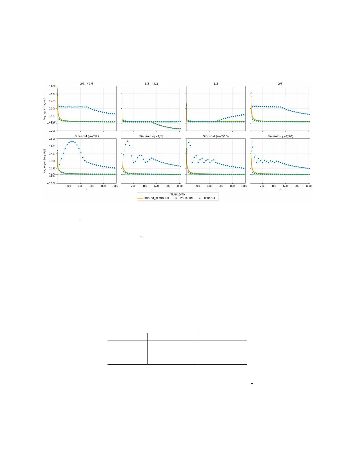
Next-T ok en Prediction and Regret Minimization Mehry ar Mohri Go ogle Researc h mohri@google.com Cla yton Sanford Go ogle Researc h chsanford@google.com Jon Sc hneider Go ogle Researc h jschnei@google.com Kiran V o drahalli Go ogle DeepMind kirannv@google.com Yifan W u ∗ Microsoft Researc h yifan.wu2357@gmail.com Abstract W e consider the question of ho w to employ next-tok en prediction algorithms in adversarial online decision making en vironments. Sp eciﬁcally , if w e train a next-token prediction model on a distribution D ov er sequences of opponent actions, when is it the case that the induced online decision making algorithm (by approximately b est responding to the model’s predictions) has lo w adv ersarial regret (i.e., when is D a low-r e gr et distribution )? F or un b ounded context windo ws (where the prediction made b y the mo del can dep end on all the actions tak en by the adv ersary th us far), w e sho w that although not ev ery distribution D is a lo w-regret distribution, every distribution D is exp onentially close (in TV distance) to one low- regret distribution, and hence sublinear regret can alw ays b e ach ieved at negligible cost to the accuracy of the original next-tok en prediction mo del. In contrast to this, for b ounded context windo ws (where the prediction made b y the mo del can dep end only on the past w actions taken b y the adversary , as ma y b e the case in mo dern transformer architectures), w e show that there are some distributions D of opp onen t pla y that are Θ(1)-far from any low-regret distribution D ′ (ev en when w = Ω( T ) and such distributions exist). Finally , we complement these results b y sho wing that the unbounded con text robustiﬁcation procedure can b e implemented by lay ers of a standard transformer architecture, and provide empirical evidence that transformer mo dels can b e eﬃciently trained to represent these new low-regret distributions. 1 In tro duction Large language mo dels are trained to p erform w ell at the task of next-token prediction: given some substring of text, estimate the conditional distribution of the next word/tok en. Increasingly , there is a fo cus on using these mo dels to p erform a far broader set of tasks, including making strategic decisions on our b ehalf [ Chen et al. , 2021 , P ark et al. , 2025 , Krishnamurth y et al. , 2024 , Nie et al. , 2025 ]. In many real applications, online decision-making is assisted with a next-token predictor. In algorithmic trading, next-tok en predictors are trained to predict market mov es (e.g., Zhang et al. 2019 , Kaggle 2018 ). The “tokens” here are not words, but the next elemen t of a market sequence, e.g., the next price mov e or order-b o ok ev ent, conditioned on the recent history . Decision makers are traders who decide p olicies with the assistance of the next-token predictor. In supply-chain and in ven tory management, decision-making is similarly assisted with demand predictors. Next-tok en predictors are trained for item-level demand tra jectories across many related pro ducts and lo cations ∗ W ork done when Yifan W u was a student researcher with Go ogle Researc h. 1 (e.g., Salinas et al. 2020 ). The “tokens” here are the next elements of an op erational sequence, e.g., the next-p erio d demand realization, replenishment arriv al. Decision makers are in ven tory planners who choose replenishmen t p olicies, e.g., order quantities, transshipmen t decisions. The pay oﬀs of the decision makers are join tly determined by their decisions and the predicted pay oﬀ-relev ant state. W e formalize the problem as training such a next-tok en predictor to play a repeated game. Ro c k-pap er-scissors is one simple example of a game. Like in next-token prediction, the decision mak er has to consider the historical actions taken in the game so far (a subsequence of tok ens) and, from this, come up with a new mixed action to tak e (a distribution o ver next tokens). If the opp onent’s actions are sto chastically drawn by nature, then it makes sense that playing w ell in this game directly corresp onds to how well our mo del can predict the next token. Ho wev er, if w e think of the tokens as the adv ersary’s actions, where things diﬀer is in ho w these tokens are generated – instead of b eing sto chastically sampled from a large data set, they are adversarially c hosen by an opp osing play er who w an ts the model to fail. One basic prop erty we might desire from these mo dels in such settings is adversarial r e gr et minimization . That is, regardless of what actions the adversary takes, our model do es at least as well as if it alwa ys play ed the b est ﬁxed action in hindsight. W e would lik e a predictor to p erform w ell when the states are sto chastically drawn, and guar- an tees regret minimization when they are adversarially generated. This raises the question: can we ac hieve a b est-of-b oth-worlds guarantee from a next-tok en predictor? Are regret minimization and next-tok en prediction compatible goals? When is it the case that training a next-token predictor on a dataset (e.g., of game transcripts) will produce a low-regret learning algorithm? Are there w ays to automatically augmen t a data set with more data so the resulting mo dels ha ve less regret? What alternatives to next-token prediction are there when training these mo dels? 1.1 Our Results W e study an online decision making setting where a decision mak er needs to tak e actions in resp onse to a c hanging state of nature (e.g. an adv ersary’s action in a game, a curren t sto c k price, etc.). The decision maker has access to a next-token prediction mo del trained on some distribution of state sequences, and would lik e use the predictions from this mo del to help them make utilit y optimizing decisions. Imp ortan tly , they would like to achiev e the b est-of-b oth-w orlds guarantee. This leads to the question of whether it is possible to r obustify a decision-mo del: tak e a model M 0 and produce a mo del M that represen ts a similar distribution ov er sequences as M 0 , while guaranteeing low regret against any adv ersary . W e pro ve the following results. • First, we remark that there exist next-tok en prediction mo dels suc h that if a decision maker ap- pro ximately b est resp onds to these predictions (e.g., via a quan tal b est resp onse), they guaran tee sublinear regret. In particular, quantal b est resp onses to the Poly a urn pro cess closely simulate the classical Hedge learning algorithm (Lemma 2.3 ) . • Second, w e p ositively answer the question of robustiﬁcation b y sho wing that giv en an y next-tok en prediction mo del M 0 it is p ossible to pro duce a mo del M such that i. quantal b est resp onses to the predictions of M lead to sublinear regret, and ii. the TV distance b etw een the distributions represen ted b y M and M 0 is arbitrarily small (Theorem 3.1 ) . 2 • W e then shift our attention to prediction mo dels with b ounded con text length (i.e., prediction mo dels whose outputs can only dep end on the previous L tokens). In contrast to the previous result, we sho w that suc h mo dels are in general impossible to robustify (Theorem 4.1 ) . Ho w ever, if the robustiﬁed mo del is allow ed to use a larger context length L ′ , it is p ossible to pro duce a robust mo del with O (1 / √ L ′ − L ) p er-round regret (Theorem 4.2 ) . • Finally , we address the question of whether it is actually p ossible to tr ain robust mo dels, with a fo cus on transformer mo dels. W e provide tw o pieces of evidence to wards an aﬃrmative answer to this question. First, we show that transformer mo dels can eﬀectively represent the robustiﬁed mo dels of Theorem 3.1 with a mild increase in size (Theorem 5.1 ) . Second, we provide exp er- imen tal evidence that it is p ossible to train small transformers to represent robustiﬁed versions of simple distributions (Section 5.2 ) . 1.2 Related W ork Our study is at the in tersection of decision-making in online learning as w ell as mo dern transformer arc hitectures in deep learning. Online Decision-Making with Finite Automata Classically , there hav e b een many studies of online decision-making for mo del families deﬁned by classes of ﬁnite automata [ Rubinstein , 1986 , Ben-p orath , 1990 , Lehrer and Solan , 2009 , Piccione and Rubinstein , 1993 ], though these earlier w orks are t ypically in the con text of repeated games (which, while related, is distinct from the online learning setting we study in this w ork). W e can view the connection to this earlier work by considering a transformer to implement a class of ﬁnite automata. Language Mo dels and Online Learning P ark et al. [ 2025 ] is a particularly relev an t mo dern study that studies the b eha vior of large language mo dels (LLMs) as game theoretic agents in b oth online learning and game theory , and is p erhaps the ﬁrst study to directly examine whether a transformer-based arc hitecture can also b e a no-regret agen t. This work focuses more on the empirical b ehavior of existing LLMs and also deﬁnes a complex regret-based training ob jectiv e by whic h to train transformers. Comparatively , we present distinct and simpler algorithms to achiev e the goal of lo w-regret transformer mo dels and present results in diﬀerent settings, fo cusing on the relation b etw een next-token-prediction and regret. Marsden et al. [ 2024 ] is another work inv estigating connections b etw een length generalization in next-token-prediction and online sequence prediction, alb eit in the sp ecialized setting of online linear dynamical systems. T ransformers for Decision Making The idea of using transformers for decision-making has also long been presen t in the deep learning literature. Chen et al. [ 2021 ] prop osed to use transformer mo dels for decision-making, and Nie et al. [ 2025 ] has built on this work in the era of large language mo dels, exploring m ultiple algorithms for transforming an existing LLM in to a mo del that can p erform in-context exploration in online decision-making settings. Krishnam urthy et al. [ 2024 ] also explores the connection b et ween LLMs and decision-making settings, but again fo cuses on existing LLMs and in v estigating m ulti-arm bandit en vironmen ts via online in-context learning. Finally , V allinder and Hughes [ 2024 ] prop oses another approach to mo dify the b ehavior of LLM agen ts in an online decision-making setting via evolving prompts. 3 2 Mo del and Preliminaries Notation W e use I [ A ] to denote the indicator function of expression A , which takes the v alue 1 when A is true, and 0 otherwise. W e generally denote sequences of elements in bolded lette rs (e.g., θ ), elemen ts of these sequences with subscripts ( θ t ), and subsegmen ts of these sequences with sup erscripts ( θ a : b = ( θ a , θ a +1 , . . . , θ b ), θ b = ( θ 1 , . . . , θ b )). F ull pro ofs are generally deferred to App endix 6 for the sake of brevity . 2.1 Next-T oken Prediction The problem of next-token pr e diction can b e formally stated as follows. W e are given a distribution D ∈ ∆(Θ T ) o ver sequences of T tok ens from an alphab et Θ. The goal is to learn a (next-token prediction) mo del M that, given as input any preﬁx token sequence θ t − 1 = ( θ 1 , . . . , θ t − 1 ), outputs the conditional distribution of the next tok en giv en this preﬁx, whic h w e denote b y M ( θ t − 1 ) ∈ ∆(Θ). W e write M ( θ | θ t − 1 ) to denote the probabilit y of a sp eciﬁc token θ ∈ Θ in the distribution M ( θ t − 1 ). By iterating the op eration of next tok en prediction, any candidate solution M to the next tok en prediction problem induces its own distribution D ( M ) ov er sequences of T tok ens. In particular, w e can deﬁne P θ T ∼ D ( M ) [ θ T ] = M ( θ 1 |∅ ) M ( θ 2 | θ 1 ) M ( θ 3 | θ 1 , θ 2 ) · · · M ( θ T | θ T − 1 ) . Con versely , every distribution D corresp onds 1 to some mo del (in the sense that it is induced b y a collection of conditional distribution functions M ( θ t | θ t − 1 )). W e can therefore measure the qualit y of a solution M to the next-token prediction problem via the TV distance d T V ( D , D ( M )) b et ween the true distribution and the distribution induced b y the mo del. Lik ewise, we can measure the similarity betw een tw o mo dels M and M ′ via the TV distance of their resp ective distributions. Bounded con text length Later in the pap er, we will consider mo dels that hav e the additional restriction of b ounde d c ontext length – that is, the mo del’s prediction M ( θ t | θ t − 1 ) for the t th token can only dep end on the w preceding tokens ( θ t − w , θ t − w +1 , . . . , θ t − 1 ) for some window size w . W e defer further discussion of b ounded context lengths to the b eginning of Section 4 . 2.2 Adv ersarial Online Decision Making The second problem we consider is that of (adversarial) online de cision making . In this problem, a de cision maker in teracts with an adversary ov er the course of T rounds. In each round t ∈ [ T ] of in teraction, the learner takes an action (sp eciﬁcally , a mixed action π t ∈ ∆( A ) supp orted on some ﬁnite action set A ) while, simultaneously , an adversary selects a state θ t ∈ Θ. As a result of this in teraction, the decision maker receives exp ected utilit y E a t ∼ π t [ U ( a, θ t )], where the utility function U : A × Θ → [ − 1 , 1] is known to all parties and ﬁxed ov er time (w e extend U linearly to mixed strategies of the decision mak er b y writing U ( π , θ ) = E a ∼ π [ U ( a, θ )]). After this in teraction, the state θ t c hosen b y the adversary is revealed to the learner, who can then use this information in the selection of their subsequent actions. The goal of the decision maker is to maximize their cumulativ e utility o ver all T rounds. Of course, the extent to whic h they can do so dep ends on the adversarial c hoices of θ t tak en by the adversary (notably , unlike in the next-token prediction problem, the sequence of states θ T = 1 F or mathematical conv enience, we will assume that all distributions D we consider hav e full supp ort – that is, ev ery sequence in Θ T app ears with some p ositiv e (alb eit p ossibly arbitrarily small) probability in the distribution. Under this assumption, this correspondence is bijective. 4 ( θ 1 , θ 2 , . . . , θ T ) is not necessarily sampled from some distribution D ). Despite this, one of the fundamen tal results in the theory of online learning sho ws that regardless of the actions taken by the adversary , it is p ossible for the decision maker to obtain sublinear r e gr et : the gap b et ween their cum ulative utilit y and the cumu lative utilit y of the b est ﬁxed action in hindsight. F ormally , giv en a sequence of (mixed) actions π = ( π 1 , . . . , π T ) and states θ = ( θ 1 , . . . , θ T ), we deﬁne the external regret as ExtReg ( π , θ ) = max a ∗ ∈ A 1 T X t [ U ( a ∗ , θ t ) − U ( π t , θ t )] . One algorithm that guarantees sublinear regret for the decision mak er is the Hedge algorithm [ F reund and Sc hapire , 1997 ]. The Hedge algorithm chooses π t so that (for an y a ∈ A ) π t ( a ) ∝ exp  1 √ T P t − 1 s =1 U ( a, θ s )  . It can b e sho wn that this guaran tees that ExtReg ( π , θ ) = O (log | A | p 1 /T ), regardless of the sequence of states chosen b y the adversary . Distinction from Bandit Setting Our setting is an online pr e diction problem rather than a bandit problem. Our motiv ation comes from decision-making with an autoregressive mo del. The autoregressiv e mak es predictions ab out the next state/token in a sequence, and the decision mak er tak es an action in resp onse to that prediction. In online prediction, the learner aims to predict the next outcome/state from a ﬁxed state space, and the decision mak er’s actions need not coincide with the state space. The actions are simply resp onses chosen giv en the predicted state under a ﬁxed pa yoﬀ function. By contrast, in bandit problems, the uncertaint y is on the pa yoﬀ of decisions: the learner chooses an action and faces unknown (or adversarial) rewards asso ciated with actions, with the central diﬃcult y b eing to learn which decisions pay oﬀs. The bandit setting is not compatible with next-token predictions. 2.3 In terpla y betw een Next-T ok en Prediction and Regret Minimization One natural wa y to apply a next-tok en prediction algorithm to the problem of online decision making is b y using it to predict the sequence of adv ersary states. In particular, the decision mak er can use an algorithm for next-token prediction to predict the next state, and then play the optimal action conditioned on this state. F ormally , for any distribution µ ∈ ∆(Θ) ov er states, let BR( µ ) = argmax a ∈ A E θ ∼ µ [ U ( a, θ )] b e the decision maker’s b est r esp onse action to this distribution. In online decision making in sto chastic settings (where the sequence of states θ is drawn from some distribution D ), b est resp onding to the predictions of an accurate mo del leads to zero external regret. Lemma 2.1. L et D ∈ ∆(Θ T ) b e a distribution over se quenc es of T states, and let M b e a next- token pr e diction mo del that has p erfe ctly le arne d the distribution D ( D ( M ) = D ). Consider the algorithm for the de cision maker which sets π t = BR ( M ( θ ( t − 1) )) (that is, the b est r esp onse to the mo del’s pr e diction of state at time t ). Then the exp e cte d r e gr et of the de cision maker on se quenc es sample d fr om D is at most zer o, i.e., E θ ∼ D [ ExtReg ( π , θ )] ≤ 0 . Ho wev er, we w ould like stronger guarantees than this – ideally , we would like to construct an online decision making algorithm with adversarial regret guarantees (e.g., those obtained b y Hedge). This leads to the question: do es there exist a distribution D where the online decision making algorithm constructed in Lemma 2.1 incurs o (1) regret against any adversary? Unfortunately , the answ er to this question is negative, as the follo wing lemma demonstrates. Lemma 2.2. L et M b e a next-token pr e diction mo del. Ther e exists a utility function U such that, if the de cision maker sets π t = BR ( M ( θ ( t − 1) )) , ther e exists an adversarial se quenc e of states θ ∈ Θ T that induc es high r e gr et, i.e., with the pr op erty that ExtReg ( π , θ ) = Ω(1) . 5 Ultimately , the negativ e result in Lemma 2.2 follo ws from the fact that the learning algorithms constructed b y best resp onding to a sequence of next-token prediction are deterministic (in the sense of alwa ys playing pure actions in A ). W e can attempt to sidestep this issue by introducing noise in the b est resp onse of the decision mak er. One natural and well-studied wa y to do this is to replace the b est resp onse with a quantal b est r esp onse 2 . Given a distribution µ ∈ ∆(Θ) ov er states and a parameter η > 0, w e deﬁne the quan tal b est response QBR( µ, η ) ∈ ∆( A ) to be the mixed action that plays action a ∈ A with probabilit y prop ortional to exp( 1 η U ( a, µ )). Note that as η → 0, this approaches the deterministic b est resp onse (and as η → ∞ , this approaches the uniform distribution ov er all actions). W e deﬁne the Polya urn mo del M Poly a to b e the following next-tok en prediction mo del: for an y t ∈ [ T ], we let M Poly a ( θ | θ ( t − 1) ) = 1 + P t − 1 s =1 I [ θ s = θ ] | Θ | + ( t − 1) . (1) In tuitively , the probabilit y of seeing a speciﬁc tok en θ at round t is roughly equal to the empirical probabilit y of observing θ in the string so far. More accurately , it is exactly the fraction of tokens equal to θ in the string Str(Θ) + θ ( t − 1) , where Str(Θ) is an arbitrary concatenation of all the tokens in Θ (it is necessary to add this additional term so that equation 1 is well-deﬁned for t = 1, and so that the induced distribution D ( M Poly a ) has full support). The following lemma sho ws that quan tal b est resp onses to predictions of the Poly a urn mo del guarantee adversarial lo w regret. Lemma 2.3. Consider the algorithm for the de cision maker which sets π t = QBR ( M Polya ( θ ( t − 1) ) , η ) , for η = 1 / √ T . Then for any adversarial se quenc e of states θ ∈ Θ T , ExtReg ( π , θ ) = O  log T + log | A | √ T  . Motiv ated by Lemma 2.3 , we formalize the prop erty of a low-regret mo del, requiring decision mak ers to achiev e low regret when quantal resp onding to next-token predictions. Deﬁnition 2.4 (Low-Regret Mo del) . We say that a next-token mo del M is a lo w-regret mo del if quantal b est r esp onses to this mo del guar ante e o (1) worst-c ase r e gr et; formal ly, for any ad- versarial se quenc e of states θ ∈ Θ T , the se quenc e of mixe d actions π ∈ ∆( A ) T deﬁne d via π t = QBR ( M ( θ t − 1 ) , 1 / √ T ) satisﬁes ExtReg ( π , θ ) = o (1) . Example (Adv ersarial Online Prediction) By selecting the utilit y function U appropriately , the online decision making framework can b e made to capture a wide range of diﬀerent p ossible applications. One particularly relev ant example (that we will use as a running example throughout the remainder of this pap er) is the problem of adversarial online pr e diction . In this problem, we set the action set A equal to the state space Θ, and deﬁne U ( a, θ ) = I [ a = θ ]; that is, the decision mak er receives a point if they successfully predict the curren t state (and receiv es zero p oints otherwise). In some later applications (e.g., the exp eriments in Section 5.2 ), w e will further insist that actions and states are binary ( A = Θ = { 0 , 1 } ). Note that in this example, the goals of the online decision maker and the next-token prediction algorithm are v ery closely aligned – they b oth wan t to pro duce go o d predictions of the next state, but with slightly diﬀeren t metrics of success (adversarial regret guaran tees versus statistical distance guaran tees). One consequence of this is that w e can directly interpret the quan tal b est resp onse as sampling from the next-token prediction mo del with temp erature η . 2 This resp onse function is also known under many other names, including softmax r esp onse , Boltzmann exploration , and multinomial lo git r esp onse . 6 3 Robustiﬁcation with Un b ounded Con text Length Lemma 2.3 demonstrates that the Poly a urn mo del is a lo w-regret mo del – following its recom- mendations (by quantally b est resp onding to them) will result in adv ersarial lo w-regret guaran tees for an online decision maker. While it is p ossible to construct other lo w-regret mo dels similarly , not every mo del is lo w-regret. F or example, the mo del M for binary states (Θ = { 0 , 1 } ) whic h alw ays predicts the next bit to b e 1 with probabilit y 1 / 3 can b e shown to incur Ω(1) regret against adv ersarial sequences of states (e.g., if the adversary selects the all-zero sequence of states θ t = 0, this mo del will never predict the next state correctly). This raises a natural question. Assume w e hav e access to a next-token mo del M 0 . Can we “robustify” our mo del and obtain a new mo del M that is b oth lo w-regret and close to the original mo del M 0 (in the sense that the distributions D 0 and D they induce are similar in TV distance)? In this section, w e answer this question aﬃrmatively . In Algorithm 1 , we give a pro cedure for taking an arbitrary next-token prediction mo del M 0 and transforming it into a low-regret next- tok en prediction mo del M . The key idea is to only mo dify the b eha vior of the mo del on preﬁxes θ t where the mo del has already incurred high regret (b y argumen ts similar to those in Lemma 2.1 , this should happ en with low probability if the sequence of states truly is sampled from D ( M 0 )). On such high-regret preﬁxes, w e instead draw the prediction of the mo del from a Poly a urn mo del, guaran teeing lo w-regret on the remainder of the time horizon. Algorithm 1 Robustiﬁcation of a next-token prediction mo del Input: Next-tok en prediction mo del M 0 implemen ting distribution D 0 , sequence of states θ t − 1 , utilit y function U : A × Θ → [ − 1 , 1], parameter α > 0. Output: Outputs M ( θ t − 1 ) for some mo del M implementing a lo w-regret distribution D . for s = 1 . . . t − 1 do Deﬁne π s ← QBR( M 0 ( θ s − 1 ) , 1 / √ T ) (the mixe d action of a quantal b est r esp onse to the original mo del) . Deﬁne π Hedge ,s ← QBR( M Poly a ( θ s − 1 ) , 1 √ T ) (the mixe d action of a quantal b est r esp onse to Polya urn mo del) Deﬁne Regret s ← ExtReg ( π s , θ s ) Deﬁne Regret Hedge ,s ← ExtReg ( π s Hedge , θ s ) if Regret s ≥ Regret Hedge ,s + 1 √ T log | A | + p 8(1 + α )(log T ) /s then ▷ (We ar e out-of-distribution, r eturn pr e diction of Polya urn mo del) return M Poly a ( θ t − 1 ) end if end for ▷ (in distribution, r eturn original mo del pr e diction) return M 0 ( θ t − 1 ) Theorem 3.1. Running Algorithm 1 on a mo del M 0 (with D 0 := D ( M 0 ) ) r esults in a r obustiﬁe d mo del M (with D := D ( M ) ) with the fol lowing pr op erties: • M is a low-r e gr et mo del with worst-c ase r e gr et O  1 √ T log( | A | · T ) + p (1 + α ) log T )  . • The TV distanc e b etwe en D and D 0 is b ounde d by d TV ( D , D 0 ) ≤ | A | T − α . Unkno wn Decisi on Problem W e note that Algorithm 1 requires the knowledge of the decision problem to calculate the regret and when to output the Poly a urn predictions. The lo w-regret guaran tee can b e generalized to the case with unknown decision problems under binary state space, whic h w e defer to Section 8 . 7 4 Robustiﬁcation with a Bounded Con text Length In the previous section, w e concerned ourselv es with next-tok en prediction models whose prediction of the state θ t at time t could dep end on all previous states θ t − 1 . In practice, most next-token predic- tion mo dels (e.g. those based on transformer architectures) are autoregressive mo dels restricted b y a context length L . That is to say , the mo del’s prediction M ( θ t | θ t − 1 ) is a round-indep endent func- tion of the previous L tok ens θ ( t − L ):( t − 1) = ( θ t − L , θ t − L +1 , . . . , θ t − 1 ). When t ≤ L , then M ( θ t | θ t − 1 ) can b e an arbitrary function of the past tokens (as in the un b ounded context case). W e will refer to such mo dels as L -b ounde d mo dels for short. As b efore, every b ounded context mo del M induces a distribution D ( M ) ov er state sequences of length T , and as b efore, we will measure the similarity of t wo models by the TV distance of their induced distributions. W e still would lik e to use these mo dels to aid in adversarial online decision making 3 . Of course, the limited context window of these mo dels constrains what regret guaran tees are p ossible. The setting of online le arning with b ounde d r e c al l studies online decision making instances where the action at round t must be a function of the previous L losses (i.e., states). It can b e sho wn [ Schneider and V o drahalli , 2024 ] that in this setting, there are simple mo diﬁcations of Hedge that guarantee at most O ( L − 1 / 2 ) regret against any adv ersary , and that this regret b ound is tight (intuitiv ely , this regret b ound is achiev able by restarting Hedge every L rounds). As in the unbounded context setting, w e can use an L -b ounded mo del M to solv e online learning with L -bounded recall by pla ying quan tal b est responses to the predictions of M . In particular, we can sho w (in analogy to Lemma 2.3 ) that there exist L -b ounded mo dels M where if the decision maker plays π t = QBR( M ( θ t − 1 ) , 1 / √ L ), the decision mak er guaran tees O (1 / √ L ) regret for themselves. W e are then faced with the same question as in the previous section: if we start with an existing L -b ounded next-token prediction mo del M 0 , can we robustify it into a mo del M that is similar to M 0 but also obtains optimal worst-case regret guarantees against an adversary? 4.1 Imp ossibilit y with the Same Con text Length W e b egin by demonstrating that, unlike in the unbounded con text setting, robustiﬁcation of b ounded context models is in general imp ossible, ev en in very simple online decision-making settings (e.g. the adversarial online prediction problem with binary states). In tuitively , this is b ecause there can exist diﬀerent L -b ounded mo dels M 0 and M 1 that induce v ery diﬀerent distributions D ( M 0 ) and D ( M 1 ) o ver sequences of length T (in particular, almost nev er agreeing ab out the next tok en), but that share the same distribution of substrings of length L . In particular, an L -b ounded mo del that can only ev er see substrings of length L will ha ve trouble distinguishing whether the state sequence is b eing generated by M 0 or M 1 . If the goal is to robustify M 0 , M then has the imp ossible tradeoﬀ b et ween playing predictions close to that of M 0 (guaran teeing lo w TV distance, but p ossibly incurring high regret with resp ect to sequences dra wn from M 1 ) or playing predictions that guaran tee lo w regret for M 1 (whic h cause a large TV distance with resp ect to M 0 ). Theorem 4.1. Set L = T / 2 , A = Θ = { 0 , 1 } , and U ( a, θ ) = I [ a = θ ] (the binary adversarial online pr e diction task). Ther e exists a c ontext length L mo del M 0 (with D 0 = D ( M 0 ) ) such that for any other c ontext length L mo del M (with D = D ( M ) ), either: 3 F or technical reasons, in this section w e will restrict ourselves to binary action settings ( | A | = 2). This has the consequence that the quantal b est resp onse function QBR( · , 1 / √ L ) has a conv ex image, which will b e imp ortan t for implementing some of the algorithms for online learning with b ounded recall (e.g., see the second-to-last line of Algorithm 2 ). 8 1. The TV distanc e d TV ( D 0 , D ) > 1 / 24 (i.e., the two mo dels ar e not close). 2. Ther e exists an adversarial se quenc e of states θ ∈ Θ T such that if π ∈ ∆( A ) T is the se quenc e of quantal b est r esp onses to M ( π t = QBR ( M ( θ t − 1 ) , 1 / √ L ) ), then ExtReg ( π , θ ) > 1 / 24 . (That is, the mo del M is not a low-r e gr et mo del). 4.2 Robustiﬁcation with a Longer Con text Length In the previous section, we sho wed that there is no wa y to robustify an existing L -b ounded mo del M 0 to a lo w-regret L -b ounded mo del M (while implementing appro ximately the same distribution). In this section, w e sho w that if w e allow the robustiﬁed mo del to hav e a sligh tly larger context windo w L ′ , we c an eﬀectiv ely p erform this robustiﬁcation. Said another wa y , this fact implies that it is p ossible to learn a mo del that will length-generalize from the distribution of a suﬃciently short sequence while maintaining no-regret guarantees in the b ounded context setting (a more realistic setting for transformer-based mo dels). W e do this by adapting the “AverageRestartHedge” algorithm of Schneider and V o drahalli [ 2024 ], which ac hieves O  1 √ m  external regret in adv ersarial online learning settings with m - b ounded recall. At a high level, this algorithm is conﬁgured with some non-constrained lo w-regret sub-algorithm (canonically , Hedge) as a subroutine. It then outputs the av erage prediction of this sub-algorithm on a uniformly randomly chosen suﬃx of the previous L losses. W e will run a v arian t of this algorithm with Algorithm 1 in place of Hedge. Sp eciﬁcally , giv en an expanded context of length L ′ , we use L out of L ′ tok ens are used for next-token prediction under the original distribution D 0 . The remaining ∆ = L ′ − L tokens can then b e viewed as the actual con text length given to the online algorithm in Schneider and V odrahalli [ 2024 ]. Our Algorithm 2 calls Algorithm 1 as a subroutine, whic h achiev es an external regret of ˜ O  1 √ ∆  (as implied b y Theorem 4.1 , it is imp ossible to get non-triv al guaran tees when ∆ = 0). Algorithm 2 Robustifying Bounded Con text Mo dels with Longer Context Lengths Input: An existing L -b ounded next-token prediction mo del M 0 , parameter α > 0, input θ L ′ . Output: A robustiﬁed L ′ -b ounded next-token prediction mo del M (with L ′ > L , ∆ = L ′ − L ). Run Algorithm 1 on M 0 with time horizon ∆ to pro duce a robustiﬁed mo del M ∆ . for m = L + 1 , . . . , L ′ do µ m ← M ∆ ( θ m : L ′ ) (i.e., the output of M ∆ on the sequence θ m , θ m +1 , . . . , θ L ) end for Cho ose a µ ∈ ∆(Θ) so that QBR( µ, 1 / √ ∆) = 1 ∆ P L ′ m = L +1 QBR( µ m , 1 / √ ∆) . return M ( θ L ′ ) = µ . Theorem 4.2. Fix L ′ > L and let ∆ = L ′ − L . Running Algorithm 2 on an L -b ounde d mo del M 0 (with D 0 := D ( M 0 ) ) r esults in a r obustiﬁe d L ′ -b ounde d mo del M (with D := D ( M ) ) with the fol lowing pr op erties: • The mo del M is a low-r e gr et mo del, with worst-c ase r e gr et  1 + ∆ T   √ 2+1 ∆ + q 8 log T +8( α +1) log ∆ ∆  . • The TV distanc e b etwe en D and D 0 is b ounde d by d TV ( D , D 0 ) ≤ ∆ − α . 9 5 T raining Lo w-Regret T ransformer Mo dels On one hand, Theorem 3.1 demonstrates that it is information theoretically p ossible to robustify any next-token prediction model M with negligible c hanges to the underlying distribution. At the same time, this raises questions ab out whether we can actually tr ain lo w-regret mo dels (after all, if d TV ( D , D 0 ) is exp onentially small, no training pro cedure can eﬃcien tly distinguish b etw een samples drawn from D and samples drawn from D 0 In this section w e in vestigate this question for the sp ecial case of tr ansformer mo dels , providing evidence that it is p ossible to directly robustify low-regret transformer mo dels. In Section 5.1 , we sho w it is p ossible to implemen t the op erations of Algorithm 1 in the logic of a standard transformer mo del (i.e., if M 0 can b e represen ted b y a small transformer, so can M ). In Section 5.2 , we pro vide exp erimen tal evidence showing that a simple masking pro cedure allows us to practically train lo w- regret transformer mo dels. 5.1 Represen ting Robustiﬁed Mo dels In this section, w e show that the representational limitations of transformers p ose no obstacle to robustiﬁcation. T o that end, w e construct a transformer that robustly predicts future states b y adding a constant n umber of lay ers to a transformer that solves next-token prediction. Theorem 5.1. Supp ose ther e exists a tr ansformer M 0 with L layers and emb e dding dimension m that exactly solves the next token pr e diction task over distribution D 0 ; that is, M 0 ( θ t | θ t − 1 ) = P D 0 [ θ t | θ t − 1 ] ). Then, ther e exists a tr ansformer M ′ with L ′ = L + 4 layers and emb e dding dimension m ′ = m + O (1) that appr oximates the output of Algorithm 1 . W e state the theorem rigorously and presen t its pro of in Section 7 . A t a high-lev el, the argumen t relies on constructing four lay ers that use the outputs of M 0 to sim ulate Algorithm 1 . Self-atten tion pla ys an essen tial role in the construction. Identifying the distribution induced by the P olya Urn strategy and calculating the t wo regret quan tities in volv e computing aggregations ov er sequences of tokens, which are naturally sim ulated with self-attention lay ers. Our construction reﬂects a realistic class of transformers by main taining tight b ounds on embedding dimension and depth and emplo ying m ulti-lay er p erceptrons that can b e compactly represented as shallow ReLU netw orks. 5.2 Empirically Robustifying Simple T ransformers In the previous sections, we demonstrated the existence of a pro cedure for learning sp ecialized lo w-regret online learning algorithms by carefully p erturbing the original statistical training data. In this section, we also demonstrate that in simple settings, it is also practically eﬃcient to train small transformers with this algorithm, suggesting that robustiﬁcation pro cedures ma y be prac- tically plausible for mo difying LLM b ehavior for decision-making while retaining go o d statistical p erformance. W e consider the sp ecial case of a decision problem to match the state. Both the action space and the state space are binary A = Θ = { 0 , 1 } , and the utility function U ( a, θ ) = I [ a = θ ]. W e conduct exp erimen ts with the minimal deco der-only transformer, NanoDO [ Liu et al. , 2024 ]. The transformer predicts a binary sequence. W e adopt the default parameters of NanoDO, with a con text length of T = 1024, 256 em b edding dimensions, 4 atten tion heads, 3 transformer blo c k la yers, and 1024 inner dimensions. W e train the transformer on three datasets with a batch size of 128. The three training processes all conv erge and stop after 500 steps. 10 BERNOULLI is the in-distribution and non-robust transformer. The dataset is generated from the distribution where the ﬁrst half of 512 bits are from Ber(1 / 3) and the second half are from Ber(2 / 3). POLYAURN is the robust transformer without distributional information. The transformer is trained on Poly a Urn sequences, where the next bit is generated from the empirical distribution in history: P [ θ t +1 = 1 | θ 1 , . . . , θ t ] = P i ∈ [ t ] θ i t . By setting the temp erature to 1 √ T , POLYAURN plays the same strategy as the Hedge algorithm. ROBUST BERNOULLI is trained on the robustiﬁed distribution of BERNOULLI . W e do this in the follo wing wa y . W e sample training data from the same distribution as BERNOULLI . W e also sample an equal num b er of P olya Urn sequences. F or a P olya Urn sequence, we keep it only if transformer BERNOULLI has a regret higher than α √ t for some t ≤ T , with α = 1 . 5. In other cases, w e discard the sequence. T o k eep the TV-distance unchanged in the training pro cess, w e mask out the loss calculation ov er the preﬁx of a P olya urn sequence, up to the ﬁrst p osition t where there is a regret higher than α √ t . By masking out the preﬁx, the transformer do es not learn the distribution that generates a high-regret preﬁx. Computational Cost Analysis. The ov erhead of robustiﬁcation of ROBUST BERNOULLI consists of: • Data generation: Sampling from both the original distribution and M Poly a is eﬃcient, requiring O ( T | Θ | ) p er sequence. F or N training sequences, total cost is O ( N T | Θ | ). • Filtering: Checking the regret condition requires computing REGRET s and REGRET HEDGE ,s for each preﬁx, which costs O ( T | A || Θ | ) p er sequence. 5.2.1 Regret Ev aluation W e ev aluate the regret of the three transformers on eight ground truth distributions o v er sequences. The bits are dra wn independently from eac h other. The ﬁrst four are static distributions where each bit is drawn from either Ber(1 / 3) or Ber(2 / 3). In the other four sim ulations, we adopt the same sim ulation setup as in Schneider and V o drahalli [ 2024 ]. The bits are generated from a p erio dically drifting distribution with P [ θ t = 1] =   sin( π / 6 + t · π /ϕ )   , for perio d ϕ ∈ { T 2 , T 5 , T 10 , T 20 } . W e ev aluate the regret of quan tal b est-resp onse by applying a soft-max la y er and setting the temperature to 1 √ T . W e estimate from 128 indep endent sequences sampled from the ground truth distribution. W e plot the regret of the three transformers in Figure 1 . The follo wing observ ations v alidate that NanoDO learns the dataset constructed by Algorithm 1 . First, the transformers eﬀectively learn to pla y the robust strategy . ROBUST BERNOULLI and POLYAURN b oth hav e v anishing regret on all eigh t ground truth data-generating pro cesses. Second, ROBUST BERNOULLI learns the switching p olicy of Algorithm 1 . ROBUST BERNOULLI preserves the same in-distribution regret of BERNOULLI in plot (1 , 2), which is negative around − 0 . 16. 5.2.2 TV-distance W e rep ort the estimated TV-distance b etw een the mo dels in T able 1 . W e estimate from 128 indep enden t sample of sequences and report the 95% conﬁdence interv al. W e also test the TV- distance b et ween t w o mo dels trained on the same BERNOULLI distribution, but with diﬀeren t random seeds. ROBUST BERNOULLI ac hieves a lo w er TV-distance than POLYAURN , where POLYAURN has a TV- distance estimated as high as 1 . 0000 from the original distribution BERNOULLI . In addition to the TV-distance, we rep ort the Next-T ok en TV-distance here. As shown in T able 1 , the full-sequence TV-distance is brutally strict and even high for tw o mo dels trained on 11 Figure 1: The regret of three transformers ov er 8 ground truth distributions. The three transformers are 1) ROBUST BERNOULLI , robustiﬁed BERNOULLI , 2) POLYAURN , and 3) BERNOULLI . The eight ground truth distributions are: a) half Ber(2 / 3) and then half Ber(1 / 3); b) half Ber(1 / 3) and half Ber(2 / 3), the same distribution that ROBUST BERNOULLI and BERNOULLI were trained on; c) Ber(1 / 3); d) Ber(2 / 3); and four p erio dically c hanging distributions on the second ro w. The plot shows (v ery narro w) conﬁdence interv als in ligh t color. BERNOULLI 1 BERNOULLI 2 BERNOULLI 1 − 0 . 4193 ± 0 . 0232 ROBUST 0 . 7602 ± 0 . 0267 0 . 6869 ± 0 . 0295 POLYAURN 1 . 0000 ± 0 1 . 0000 ± 0 T able 1: The TV-distance b etw een transformers. BERNOULLI i are tw o mo dels trained on the same Ber(1 / 3) → Ber(2 / 3) pro cess with diﬀeren t random seeds. W e refer to ROBUST BERNOULLI as ROBUST . 12 the same distribution. Tin y p er-token diﬀerences are calculated as a diﬀerence across the entire sequence. Ev en models that b ehav e similarly at a tok en lev el can ha ve a high TV-distance on whole sequences. Per-step TV instead measures the lo cal diﬀerence of the t wo predictiv e mo dels at each preﬁx. W e deﬁne the following Next-T ok en TV-distance. F or eac h preﬁx θ s , w e can calculate the TV- distance of the next-token prediction, d TV ( M 1 ( ·| θ s ) , M 2 ( ·| θ s )). The Next-T oken TV-distance d NT tak es the exp ectation of the preﬁx from the distribution of BERNOULLI , i.e., with the ﬁrst T / 2 drawn from Ber(1 / 3) and the second T / 2 tokens from Ber(2 / 3): d NT = E θ ∼ BERNOULLI h 1 T P s ∈ [ T ] d TV ( M 1 ( ·| θ s ) , M 2 ( ·| θ s )) i . W e rep ort the Next-T oken TV-distance in T able 2 . The results are calculated with 128 inde- p enden t draws of a sequence. BERNOULLI 1 BERNOULLI 2 BERNOULLI 1 − 0 . 0156 ROBUST 0 . 0199 ± 0 . 0001 0 . 0299 ± 0 . 0001 POLYAURN 0 . 1529 ± 0 . 0003 0 . 1655 ± 0 . 0004 T able 2: Next-T ok en TV distance b etw een transformers. BERNOULLI i are t wo mo dels trained on the same Ber(1 / 3) → Ber(2 / 3) pro cess with diﬀerent random seeds. W e refer to ROBUST BERNOULLI as ROBUST . 13 References E. Ben-p orath. The complexity of computing a b est resp onse automaton in rep eated games with mixed strategies. Games and Ec onomic Behavior , 2(1):1–12, Marc h 1990. doi: None. URL https://ideas.repec.org/a/eee/gamebe/v2y1990i1p1- 12.html . 3 E. Candes and T. T ao. Deco ding b y linear programming, 2005. URL math/0502327 . 26 L. Chen, K. Lu, A. Ra jeswaran, K. Lee, A. Grov er, M. Laskin, P . Abb eel, A. Sriniv as, and I. Mordatch. Decision transformer: Reinforcement learning via sequence mo deling, 2021. URL https://arxiv.org/abs/2106.01345 . 1 , 3 Y. F reund and R. E. Sc hapire. A decision-theoretic generalization of on-line learning and an application to b o osting. Journal of c omputer and system scienc es , 55(1):119–139, 1997. 5 L. Hu and Y. W u. Predict to minimize swap regret for all pa yoﬀ-bounded tasks. In 2024 IEEE 65th A nnual Symp osium on F oundations of Computer Scienc e (FOCS) , pages 244–263. IEEE, 2024. 30 Kaggle. Tw o sigma: Using news to predict stock mo vemen ts. Kaggle Comp etition, 2018. URL https://www.kaggle.com/c/two- sigma- financial- news . Comp etition host: Tw o Sigma. Ac- cessed 2026-01-28. 1 B. Kleinberg, R. P . Leme, J. Schneider, and Y. T eng. U-calibration: F orecasting for an unknown agen t. In The Thirty Sixth A nnual Confer enc e on L e arning The ory , pages 5143–5145. PMLR, 2023. 27 , 29 , 30 A. Krishnamurth y , K. Harris, D. J. F oster, C. Zhang, and A. Slivkins. Can large language mo dels explore in-context?, 2024. URL . 1 , 3 E. Lehrer and E. Solan. Approachabilit y with b ounded memory . Games and Ec onomic Behav- ior , 66(2):995–1004, July 2009. doi: None. URL https://ideas.repec.org/a/eee/gamebe/ v66y2009i2p995- 1004.html . 3 Y. Li, J. D. Hartline, L. Shan, and Y. W u. Optimization of scoring rules. In Pr o c e e dings of the 23r d A CM Confer enc e on Ec onomics and Computation , pages 988–989, 2022. 29 P . J. Liu, R. Nov ak, J. Lee, M. W ortsman, L. Xiao, K. Everett, A. A. Alemi, M. Kurzeja, P . Marcenac, I. Gur, S. Korn blith, K. Xu, G. Elsay ed, I. Fischer, J. P ennington, B. Adlam, and J.-S. Dickstein. Nano do: A minimal transformer deco der-only language mo del implementa- tion in JAX., 2024. URL http://github.com/google- deepmind/nanodo . 10 A. Marsden, E. Dogariu, N. Agarwal, X. Chen, D. Suo, and E. Hazan. Pro v able length generalization in sequence prediction via sp ectral ﬁltering, 2024. URL . 3 S. Mendelson, A. P a jor, and N. T omczak-Jaegermann. Reconstruction and subgaussian op erators in asymptotic geometric analysis. Ge ometric and F unctional Analysis , 17:1248–1282, 11 2007. doi: 10.1007/s00039- 007- 0618- 7. 26 14 A. Nie, Y. Su, B. Chang, J. N. Lee, E. H. Chi, Q. V. Le, and M. Chen. Evolv e: Ev aluating and optimizing llms for in-context exploration, 2025. URL . 1 , 3 C. Park, X. Liu, A. Ozdaglar, and K. Zhang. Do llm agen ts hav e regret? a case study in online learning and games, 2025. URL . 1 , 3 M. Piccione and A. Rubinstein. Finite automata play a rep eated extensiv e game. Journal of Ec onomic The ory , 61(1):160–168, 1993. ISSN 0022-0531. doi: https://doi.org/10.1006/jeth.1993. 1063. URL https://www.sciencedirect.com/science/article/pii/S002205318371063X . 3 A. Rubinstein. Finite automata play the rep eated prisoner’s dilemma. Journal of Ec onomic The ory , 39(1):83–96, June 1986. doi: None. URL https://ideas.repec.org/a/eee/jetheo/ v39y1986i1p83- 96.html . 3 D. Salinas, V. Flunkert, J. Gasthaus, and T. Janusc howski. Deepar: Probabilistic forecasting with autoregressiv e recurren t netw orks. International journal of for e c asting , 36(3):1181–1191, 2020. 2 C. Sanford, D. J. Hsu, and M. T elgarsky . Represen tational strengths and limitations of transformers. In A. Oh, T. Naumann, A. Glob erson, K. Saenko, M. Hardt, and S. Levine, editors, A dvanc es in Neur al Information Pr o c essing Systems , v olume 36, pages 36677–36707. Curran Asso ciates, Inc., 2023. 25 , 26 C. Sanford, D. Hsu, and M. T elgarsky . T ransformers, parallel computation, and logarithmic depth. In R. Salakh utdinov, Z. Kolter, K. Heller, A. W eller, N. Oliver, J. Scarlett, and F. Berkenk amp, editors, Pr o c e e dings of the 41st International Confer enc e on Machine L e arning , v olume 235 of Pr o c e e dings of Machine L e arning R ese ar ch , pages 43276–43327. PMLR, 21–27 Jul 2024. URL https://proceedings.mlr.press/v235/sanford24a.html . 21 J. Schneider and K. V o drahalli. Online learning with b ounded recall. In Pr o c e e dings of the 41st International Confer enc e on Machine L e arning , pages 43791–43803, 2024. 8 , 9 , 11 , 21 A. V allinder and E. Hughes. Cultural ev olution of co op eration among llm agents, 2024. URL https://arxiv.org/abs/2412.10270 . 3 Z. Zhang, S. Zohren, and S. Rob erts. Deeplob: Deep conv olutional neural netw orks for limit order b o oks. IEEE T r ansactions on Signal Pr o c essing , 67(11):3001–3012, 2019. 1 15 6 Omitted Pro ofs 6.1 Pro of of Lemma 2.1 Pr o of. Let h t − 1 := ( θ 1 , . . . , θ t − 1 ) denote the history up to time t − 1. By assumption, the mo del’s next token prediction is the true conditional probability at ev ery history: M ( h t − 1 ) = D ( · | h t − 1 ) . A t round t , the decision maker pla ys the b est resp onse to this next-token prediction: π t ∈ BR  M ( h t − 1 )  ∈ arg max π ∈ ∆( A ) E θ t ∼ D ( ·| h t − 1 )  U ( π , θ t )  . F or an y other action a ∗ ∈ A . By the optimality of π t under the correct conditional, E  U ( π t , θ t )   h t − 1  ≥ E  U ( a ∗ , θ t )   h t − 1  . T aking exp ectations ov er h t − 1 and using the tow er prop ert y yields E  U ( π t , θ t )  ≥ E  U ( a ∗ , θ t )  . Summing ov er t = 1 , . . . , T giv es E θ ∼ D h T X t =1 U ( π t , θ t ) i ≥ E θ ∼ D h T X t =1 U ( a ∗ , θ t ) i for every a ∗ ∈ A. Equiv alently , the exp ected (av erage) utility r e gr et v ersus the b est ﬁxed action in hindsight is ≤ 0: E θ ∼ D " max a ∗ ∈ A 1 T T X t =1  U ( a ∗ , θ t ) − U ( π t , θ t )  # ≤ 0 , whic h is precisely E θ ∼ D [ ExtReg ( π , θ )] ≤ 0. 6.2 Pro of of Lemma 2.2 Pr o of. Consider the binary token space and action space Θ = A = { 0 , 1 } , with utilit y function U ( a, θ ) = I [ a = θ ]. Fix an y next-tok en mo del M and the induced (deterministic) decision rule π t = BR( M ( θ ( t − 1) )), which is a deterministic function of the history h t − 1 = ( θ 1 , . . . , θ t − 1 ). Deﬁne an adversary that, after observing a t (or equiv alen tly inferring a t from the history), sets θ t = 1 − a t . Then the learner obtains zero utility eac h round: U ( a t , θ t ) = 0 for all t, so P T t =1 U ( a t , θ t ) = 0. On the other hand, for the realized state sequence θ 1: T , the b est ﬁxed action in hindsight is the ma jorit y elemen t of the sequence, which ac hieves utility at least T / 2. Therefore, ExtReg ( π , θ ) = 1 T max a ∈{ 0 , 1 } T X t =1 U ( a, θ t ) − T X t =1 U ( a t , θ t ) ! ≥ 1 2 . Th us, the regret is b ounded b elow b y a constant, i.e. Ω(1). 16 6.3 Pro of of Lemma 2.3 Pr o of of L emma 2.3 . Fix a ﬁnite action set A and utilities U : A × Θ → [ − 1 , 1]. At round t , the P olya urn predictor is M Poly a ( θ | θ 1: t − 1 ) = 1 + P t − 1 s =1 I [ θ s = θ ] | Θ | + ( t − 1) . The QBR with parameter η > 0 pla ys π t ( a ) ∝ exp  1 η U  a, M Poly a ( · | θ 1: t − 1 )   , where exp  1 η U  a, M Poly a ( · | θ 1: t − 1 )   = exp  1 η ( | Θ | + t − 1) h X θ ∈ Θ U ( a, θ ) + t − 1 X s =1 U ( a, θ s ) i . Th us, QBR plays π t ( a ) ∝ exp  C ( a ) η ( | Θ | + t − 1)  · exp  1 η ( | Θ | + t − 1) t − 1 X s =1 U ( a, θ s )  . Th us π t is an exp onential-weights distribution o ver actions with round- t learning rate λ t := 1 η ( | Θ | + t − 1) applied to the realized utilities U ( a, θ s ), and with an action-dep enden t prior factor that only changes b y a common (rescaling-inv arian t) temp erature at each t . Standard analysis of Hedge with time- v arying learning rates (apply , e.g., the p oten tial argumen t round by round) gives, for an y adv ersarial sequence θ 1: T , T X t =1  U ( π t , θ t ) − U ( a ⋆ , θ t )  ≥ − ln | A | λ T − 1 2 T X t =1 λ t , for all a ⋆ ∈ A, using U ∈ [ − 1 , 1]. Cho osing η = T − 1 / 2 (as in the statement) yields λ t = √ T | Θ | + t − 1 , so 1 T T X t =1  U ( a ⋆ , θ t ) − U ( π t , θ t )  ≤ ln | A | T λ T + 1 2 T T X t =1 λ t = ln | A | √ T + O  log T √ T  = O  log T + ln | A | √ T  . whic h implies the regret b ound ExtReg ( π , θ ) = O  log T +ln | A | √ T  . 6.4 Pro of of Theorem 3.1 Pr o of. Let E b e the even t that for some s ∈ [ T − 1], Regret s ≥ Regret Hedge ,s + 1 √ T log | A | + p 8(1 + α )(log T ) /s (i.e., w e return M Poly a ( θ t − 1 ) for all rounds t > s ). Let τ b e the random v ariable representing the minimum such s ; if the even t E does not o ccur, let τ = T . 17 W e b egin by proving that the new mo del M implemen ts a low-regret distribution D . Fix any adv ersarial sequence of states θ and deﬁne π t = QBR( M ( θ t − 1 ) , 1 / √ T ). W e can decomp ose the external regret ExtReg ( π , θ ) via ExtReg ( π , θ ) = max a ∗ ∈ A 1 T  τ X t =1 [ U ( a ∗ , θ t ) − U ( π t , θ t )] + T X t = τ +1 [ U ( a ∗ , θ t ) − U ( π t , θ t )]  By assumption, for t ≤ τ , M ( θ t − 1 ) = M 0 ( θ t − 1 ), and so P τ t =1 [ U ( a ∗ , θ t ) − U ( π t , θ t )] ≤ τ Regret τ . By the deﬁnition of τ , Regret τ < Regret Hedge ,s + 1 √ T log | Θ | + p 8(1 + α )(log T ) /τ , and so w e in turn ha ve that P τ t =1 [ U ( a ∗ , θ t ) − U ( π t , θ t )] ≤ τ  Regret Hedge ,s + 1 √ T log | Θ | + p 8(1 + α )(log T ) /τ  = τ Regret Hedge ,s + O  √ T  log | Θ | + p (1 + α ) log T  . F or t > τ , w e hav e that M ( θ t − 1 ) = M Poly a ( θ t − 1 ). By Lemma 2.3 , w e therefore ha ve that τ Regret Hedge ,s + P T t = τ +1 [ U ( a ∗ , θ t ) − U ( π t , θ t )] = O  T · log( T )+log | A | √ T  = O ( √ T log ( | A | · T )). Com- bining these tw o terms, we hav e that ExtReg ( π , θ ) = O  1 √ T (log( | A | · T ) + p (1 + α ) log T )  = o (1). W e next b ound the TV-distance b etw een D and D 0 . Note that b ecause we pla y the recommen- dation of M 0 (and sample from D 0 ) un til even t E o ccurs, the TV distance d TV ( D , D 0 ) is upp er b ounded by the probability P θ ∼ D 0 [ E ] of this even t. T o do this, we begin by deﬁning a to be the sequence of pure action b est resp onses to the recommendations of M 0 ; i.e., a t = BR( M 0 ( θ t − 1 )). W e argue that if θ is truly sampled from D 0 , then a and π obtain similar utilities and hence similar regrets. W e can quantitativ ely b ound this through the following lemma. Lemma 6.1. L et µ ∈ ∆(Θ) b e a distribution over states θ . L et a = BR ( µ ) and π = QBR ( µ, η ) . Then U ( a, µ ) − U ( π , µ ) ≤ η log | A | . Pr o of. Note that we can equiv alen tly deﬁne the quantal b est resp onse π as the mixed action that maximizes the regularized utilit y V ( π ) = U ( π , µ ) + η H ( π ) (where H is the en tropy function). W e therefore hav e that V ( a ) ≤ V ( π ); expanding this out (and using the fact that H ( a ) = 0), we ﬁnd that U ( a, µ ) ≤ U ( π , µ ) + η H ( π ) ≤ U ( π , µ ) + η log | A | , from which the conclusion follows. F rom Lemma 6.1 , it follo ws that when θ ∼ D 0 , E θ t [ U ( a t , θ t ) − U ( π t , θ t )] ≤ (log | A | ) / √ T . Secondly , since a t is the b est resp onse to the distribution of θ t , for an y action a ∗ t w e ha ve that E θ t [ U ( a ∗ t , θ t ) − U ( a t , θ t )] ≤ 0. Combining these expressions, w e ha ve that E θ t [ U ( a ∗ t , θ t ) − U ( π t , θ t )] ≤ (log | A | ) / √ T . Let R t ( a ∗ ) = P t ( U ( a ∗ , θ t ) − U ( π t , θ t )) b e the unnormalized regret at time t with resp ect to a ∗ , and similarly R Hedge ,t ( a ∗ ) = P t ( U ( a ∗ , θ t ) − U ( π Hedge ,t , θ t )). By the previous observ ation, R t ( a ∗ ) − R Hedge ,t ( a ∗ ) − t (log | A | ) / √ T is a super-martingale, so b y Azuma’s inequalit y , w e hav e that 18 P  R t ( a ∗ ) ≥ R Hedge ,t ( a ∗ ) + t log | A | √ T + C  ≤ exp  − C 2 8 t  . Substituting C = p 8(1 + α )(log T ) t (and normalizing by t ), we ﬁnd that P  1 t R t ( a ∗ ) ≥ R Hedge ,t ( a ∗ ) + log | A | √ T + r 8(1 + α )(log T ) t  ≤ T − (1+ α ) . No w, Regret t = max a ∗ 1 t R t ( a ∗ ). Applying a union b ound ov er all t ∈ [ T ] and a ∗ ∈ | A | , w e ha ve that P [ E ] ≤ | A | · T − α , as desired. 6.5 Pro of of Theorem 4.1 T o formally construct these tw o mo dels M 0 and M 1 , we will make use of the theory of de Bruijn se quenc es . The de Bruijn gr aph ˆ G σ,k of order k on an alphab et Θ = { s 1 , . . . , s | Θ | } of size | Θ | is a directed graph whose v ertices represent all distinct sequences of length k − 1. F or ev ery sequence s i 1 s i 2 . . . s i k of length k , there is a directed edge from the v ertex s i 1 s i 2 . . . s i k − 1 to the v ertex s i 2 s i 3 . . . s i k . A de Bruijn se quenc e of order k is a cyclic sequence of characters in Θ where eac h of the p ossible | Θ | k substrings of length k appears exactly once. Note that a de Bruijn sequence of order k corresp onds to a (lo op-remov ed) Eulerian cycle in a de Bruijn graph of order k (whic h in turn must exist since ev ery no de in ˆ G σ,k has equal indegree and outdegree | Θ | ). Giv en a ﬁxed de Bruijn sequence of order L and ov er a binary alphabet Θ = { 0 , 1 } , we can use it to construct tw o nearly deterministic L -b ounded mo dels M 0 and M 1 . M 0 and M 1 induce the same uniform marginal distribution ov er length L substrings, but the next-token predictions are diﬀerent. W e construct in the following wa y: we deﬁne M 0 ( θ L ) sp eciﬁed by the deterministic next-tok en of the de Bruijn sequence, and M 1 ( θ L ) = 1 − M 0 ( θ L ) as the deterministic opp osite of M 1 . The ﬁrst L tokens in the Mark ov pro cess are seeded uniformly so that b oth pro cesses remain in the same stationary distribution: the marginal distribution ov er any t > L substring is uniform. Th us, any context length L mo del M will not b e able to distinguish M 0 from M 1 . Suc h a mo del M makes predictions v ery diﬀerently from the deterministic next-token of either M 0 or M 1 , leading to Theorem 4.1 . Pr o of. W e will prov e this by constructing tw o L -b ounded mo dels M 0 and M 1 with the following guaran tee: for any other L -b ounded mo del, d T V ( D 0 , D ) + E θ ∼ D 1 [ ExtReg ( π , θ )] ≥ 1 / 12 . The theorem statement then follo ws from this guaran tee (if E θ ∼ D 1 [ ExtReg ( π , θ )] ≥ 1 / 24, there exists some sequence in the supp ort of D 1 that realizes this). W e ﬁrst describ e the tw o mo dels. These models will b e (nearly) deterministic Marko v pro cesses of order L . F or b oth M 0 and M 1 , we set probabilities for the ﬁrst L tokens so that each token is equally likely to b e 0 or 1 (i.e., for t ≤ w , M 0 ( θ t | θ t − 1 ) = M 1 ( θ t | θ t − 1 ) = Unif( { 0 , 1 } )). W e then use a de Bruijn sequence to set the transition probabilities of M 0 and M 1 as follows. Pic k an arbitrary binary de Bruijn sequence of order L . F or an L -tuple of states θ L = ( θ 1 , . . . , θ L ), let DB( θ L ) ∈ { 0 , 1 } b e the token immediately following θ L in this de Bruijn sequence. Then: 19 • F or M 0 , set M 0 ( θ t | θ ( t − L ):( t − 1) ) = I  θ t = DB( θ ( t − L ):( t − 1) )  . • F or M 1 , set M 1 ( θ t | θ ( t − L ):( t − 1) ) = I  θ t = 1 − DB( θ ( t − L ):( t − 1) )  . That is, we deterministically 4 set M 0 to generate the next bit by follo wing the de Bruijn sequence, and set M 1 to generate the next bit b y deterministically following the opp osite of the de Bruijn sequence. W e b egin by making the following observ ation: for b oth Marko v pro cesses M 0 and M 1 , the uniform distribution ov er L -bit strings is a stationary distribution for the pro cess. This follo ws b ecause the induced Marko v chain o ver L -bit strings is doubly sto chastic for b oth M 0 and M 1 (for an y state θ L , there are exactly t wo predecessor states that can lead to it, one from the de Bruijn sequence, and one not from it). This means that for all t > L , the distribution of θ ( t − L ):( t − 1) is uniform ov er Θ L . No w let us consider the candidate robust L -b ounded mo del M (with distribution D ( M ) = D ). W e will call an L -tuple of states θ L ∈ Θ L high-r e gr et if M (DB( θ L ) | θ L ) ≥ 2 / 3, and let α ∈ [0 , 1] equal the fraction of tuples in Θ L that are high-regret. Note that on a high-regret sequence the prediction of M disagrees with that of M 1 , and will cause M to incur external regret on sequences dra wn from D 1 . In particular, we ﬁrst claim that E θ ∼ D 1 [ ExtReg ( π , θ )] ≥ 1 3 α − (1 − α ). T o see this, w e will compare the expected utility of following the baseline strategy π ∗ = (1 / 2 , 1 / 2) to the utilit y of follo wing the sequence of recommendations π t = QBR( M ( θ t − 1 ) , 1 / √ L ). The baseline strategy has the prop erty that U ( π ∗ , θ ) = 1 / 2 regardless of θ , so the cumulativ e utility of the baseline is alwa ys T / 2. If θ ( t − L ):( t − 1) is a high-regret tuple, then π t will equal DB( θ ( t − L ):( t − 1) ) with probabilit y at least 2 / 3 (this probability only gets ampliﬁed b y the quan tal b est resp onse), and therefore U ( π t , θ t ) ≤ 1 / 3. On the other hand, if θ ( t − L ):( t − 1) is not a high-regret tuple, then we only ha ve the trivial b ound U ( π t , θ t ) ≤ 1. Finally , for any t < L , θ t will b e drawn uniformly from { 0 , 1 } , so the exp ected utility E [ U ( π t , θ t )] = 1 / 2. Com bining these facts (and using the fact that for eac h t > L , θ ( t − L ):( t − 1) is drawn uniformly from Θ L and therefore has an α probability of b eing high-regret), we ﬁnd that E θ ∼ D 1 [ ExtReg ( π , θ )] ≥ E θ ∼ D 1 " 1 T T X t =1 U ( π ∗ , θ t ) − U ( π t , θ t ) # ≥ ( T − L ) T ·  1 2 − α 3 − (1 − α )  = α 3 − 1 4 . On the other hand, we will show that if α is to o small, then the TV distance b et ween D 0 and D is necessarily large. Indeed, let ˜ D 0 and ˜ D b e the distributions of the ﬁrst L + 1 states from D 0 and D resp ectiv ely – by the data-pro cessing inequality , d TV ( D 0 , D ) ≥ d TV ( ˜ D 0 , ˜ D ). But we can directly b ound d TV ( ˜ D 0 , ˜ D ) ≥ (1 − α ) / 3, since if θ 1: L is not high-regret (which happ ens with probability 1 − α ), with probability at least 1 / 3 M ( θ 1: L ) will not equal DB( θ 1: L ) and thus generate a sequence lying outside the supp ort of M 0 . It follo ws that d T V ( D 0 , D ) + E θ ∼ D 1 [ ExtReg ( π , θ )] ≥ 1 / 12, as desired. 4 If we wan t to ensure D 0 and D 1 ha ve full supp ort, w e can add inﬁnitesimal mass on the other option (i.e. follow the de Bruijn sequence with probabilit y 1 − ϵ , follow the opp osite with probabilit y ϵ ). This do es not aﬀect any of the subsequen t logic. 20 6.6 Pro of of Theorem 4.2 Pr o of of The or em 4.2 . First, we b ound the TV distance b etw een D and D 0 . F ollo wing the pro of of Theorem 3.1 , for any substring of length m ≤ ∆, the probabilit y that Algorithm 1 plays the out-of-distribution prediction is b ounded by 1 T · 1 ∆ α +1 . There are at most ∆ T substrings of length b ounded by ∆. Applying a union b ound we prov e the TV distance result. The external regret b ound follows from the same pro of in Schneider and V o drahalli [ 2024 ]. W e write the proof here. Given a context of length L , the output of Algorithm 2 can b e view ed as the uniform combination of ∆ copies of Algorithm 1 , each starting at a time m = L + 1 , . . . , L ′ . In tuitively , Algorithm 2 inherits the regret of Algorithm 1 ov er length ∆ strings with the given parameters, which is b ounded by √ 2+1 ∆ + q 8 log T +8( α +1) log ∆ ∆ . W e denote Algorithm 1 by A and its regret by Regret A . First, we introduce notation related to oﬀsets. F or an y t ∈ − (∆ − 1) , T − 1 and m ∈ [∆], w e write ˜ a m t = a m t + m = A ( θ t , . . . , θ t + m − 1 ) , whic h is the prediction by the m -th copy of A ab out state θ t + m . No w w e rearrange the total pay oﬀ of Algorithm 2 and write it in copies of A : X t I [ a t = θ t ] = T X t =1 1 ∆ ∆ X m =1 I [ a m t = θ t ] = T X t =1 1 ∆ ∆ X m =1 I  ˜ a m t − m = θ t  = T − 1 X t = − ∆+1 1 ∆ ∆ X m =1 I [˜ a m t = θ t + m ] ≥ T − 1 X t = − ∆+1 1 ∆ " max θ ∈{ 0 , 1 } t +∆ X m = t I [ θ = θ m ] − ∆ Regret A # ≥ max θ ∈{ 0 , 1 } T X t =1 I [ θ = θ t ] − ( T + M ) Regret A . Normalizing b oth sides by 1 T , we prov e the theorem. 7 T ransformer Robustiﬁcation Construction 7.1 T ransformer Preliminaries W e in tro duce a formal mo del of a transformer, drawing hea vily from Sanford et al. [ 2024 ]. F or a sequence of queries, k eys, and v alues Q, K, V ∈ R T × m , an autor e gr essive self-attention he ad of em b edding dimension m with softmax attention is deﬁned b y f ( Q, K, V ) = softmax( QK T ) V , where the softmax op erator softmax( v ) = 1 P T i =1 exp( v i ) (exp( v 1 ) , . . . , exp( v T )) 21 is applied row-wise, and mask M ∈ R T × T satisﬁes M i,j = ( 0 if i ≥ j, −∞ otherwise. Multi-he ade d attention concatenates the outputs for m ultiple attention heads. F or some se- quen tial input X ∈ R T × m , an H - headed attention unit computes H queries, k eys, and v alues of em b edding dimension m H as Q h = X W h Q , K h = X W k K , V h = X W h V , for pro jections W h Q , W h K , W h V ∈ R m × m/H , for every h ∈ [ H ]. The output of the resulting H -headed atten tion la yer is the following: X 7→ [ f ( Q 1 , K 1 , V 1 ) . . . f ( Q H , K H , V H )] , for parameters ( W h Q , W h K , W h V ) h ∈ [ H ] . W e deﬁne a tr ansformer of depth L as a function of the form g = ϕ L ◦ f L ◦ · · · ◦ ϕ 1 ◦ f 1 ◦ ϕ 0 , where f 1 , . . . , f L are multi-headed attention lay ers of embedding dimension m , and ϕ 1 , . . . , ϕ L − 1 : R m → R m are multi-layer p er c eptr ons applied elemen t-wise, i.e. ϕ ℓ ( X ) = ( ϕ ℓ ( X 1 ) , . . . ϕ ℓ ( X T )) , ϕ 0 : Σ → R m is an em b edding lay er from some alphabet Σ, and ϕ L : R m → R d out is an output MLP lay er. In the subsequen t pro of, w e argue informally that our MLP units can be eﬃciently constructed as a shallo w ReLU net w ork with bounded width (t ypically , logarithmic in sequence length T ) and bit-precision (log ( T ) as well). W e assume that the alphab et Σ enco des a p ositional enco ding. That is, in the pro of of Theo- rem 5.1 , we let Σ = Θ × [ T ] and enco de the input sequence θ T ∈ Θ T as (( θ 1 , 1) , . . . , ( θ T , T )). W e assume that there exists a constan t “b eginning-of-sequence tok en” X BOS that produces constant k ey and v alue vectors and can b e attended to. 7.2 Pro of of Theorem 5.1 W e restate Theorem 5.1 precisely . Theorem 7.1. Supp ose ther e exists a tr ansformer g M 0 of depth L and emb e dding dimension m that exactly c omputes the next-token pr ob abilities over some distribution D 0 (i.e. for any θ T ∈ Θ T , g M 0 ( θ T ) t,i = P D 0 [ θ t = i | θ t − 1 ] ). Supp ose the loss function U is Lipschitz and c an b e exactly r ep- r esente d by a multi-layer p er c eptr on with width indep endent of T . Then, ther e exists a tr ansformer g ′ of depth L ′ = L + 4 , he ads H ′ = O ( | A | 2 ) , and emb e dding dimension m ′ = m + O ( | A | 3 + | Θ | ) such that the fol lowing is true (in the notation of A lgorithm 1 ) for some err or term δ ≤ 1 T c (for any ﬁxe d c > 0 ), for al l t ≤ T : 1. If ther e exists s ≤ t − | A | such that Regret s ≥ Regret Hedge ,s + 1 √ T log | A | + p 8(1 + α )(log T ) /s + δ, then g ′ ( θ T ) t = M Polya ( θ ( t − 1) ) . 22 2. If every s ≤ t − | A | satisﬁes Regret s < Regret Hedge ,s + 1 √ T log | A | + p 8(1 + α )(log T ) /s − δ, then g ′ ( θ T ) t = M 0 ( θ t − 1 ) = g M 0 ( θ T ) . Before pro ving Theorem 7.1 , we observe that there are t wo senses in whic h the transformer construction is approximate: • The Regret s condition makes no guarantees within an additive in terv al of width 2 δ . • The transformer guarantee do es not account for the previous | A | states in the outcomes. Both issues are insigniﬁcan t in the regime where T is large, and Theorem 3.1 could b e adapted in a straightforw ard manner to accommo date these changed conditions. Pr o of. W e transformer g ′ b y in tro ducing six gadgets. Assume that A = { 1 , . . . , k } throughout. 1. The ﬁrst L la yers of g ′ exactly compute the output of g M 0 . Concretely , w e assume that the t th output of the L th lay er exactly enco des a p ositional embedding u t , the input state θ t − 1 , and the next token distribution under D 0 : p t =  P D 0 [ θ t = θ | θ t − 1 ]  θ ∈ Θ ∈ R | Θ | . The output MLP computes the exp ected loss of each action with resp ect to p t : ℓ t a = E θ ∼ p t [ U ( a, θ )] , for eac h a ∈ A. 2. An additional head in lay er L computes M Poly a ( θ ( t − 1) ) = 1 + P t − 1 s =1 I [ θ s = θ ] | Θ | + ( t − 1) ! θ ∈ Θ in the t th output b y calculating a rolling av erage with the self-attention head. The output MLP computes ℓ Hedge ,t a = E θ ∼M Poly a ( θ ( t − 1) ) [ U ( a, θ )] , for each a ∈ A. 3. k − 1 heads in lay er L + 1 jointly retriev e the pairs of partial losses ( ℓ t − k +1 1 , ℓ Hedge ,t − k +1 1 ) , ( ℓ t − k +2 2 , ℓ Hedge ,t − k +2 2 ) , . . . , ( ℓ t − 1 k − 1 , ℓ Hedge ,t − 1 k − 1 ) from the k previous tokens. 4. La y er L + 2 uses k 2 atten tion heads to compute each comp onent of b oth QBRs. π t − k a = exp( √ T ℓ t − k a ) P a ′ exp( √ T ℓ t − k a ′ ) , π Hedge ,t − k a = exp( √ T ℓ Hedge ,t − k a ) P a ′ exp( √ T ℓ Hedge ,t − k a ′ ) . 23 5. La y er L + 3 uses one head to compute Regret t − k − Regret Hedge ,s b y av eraging the QBR losses, and ev aluate whether the inequality condition holds for t − k . 6. La y er L + 4 detects whether the inequality condition o ccurs for any s ≤ t − k b y computing an OR ov er the inequality conditions. While the pro of do es not formally deﬁne all weigh ts in the mo del, we outline how eac h gadget is constructed in the following sections. W e fo cus in greatest sp eciﬁcity on the attention patterns that construct the aggregations employ ed by diﬀerent gadgets. W e also provide brief justiﬁcations for why all MLPs can b e compactly constructed and a high-level error analysis. Gadget 1: Next-tok en probabilities (La y ers 1 to L ). The relative sizes of the tw o mo dels immediately imply that the ﬁrst L la yers of g ′ can exactly simulate g M 0 . The residual connections in g ′ (and the sligh t increase in embedding dimension) mak e it p ossible for g ′ to preserve a positional enco ding u t and θ t − 1 throughout the L lay ers, even if the residual stream of g M 0 “forgets” them. Because ℓ t a is a linear function of p t , it can b e trivially computed with a linear lay er of the L th la yer’s MLP ϕ L . The MLP additionally computes ( I [ θ t − 1 = θ ]) θ ∈ Θ ∈ { 0 , 1 } k , whic h emplo ys k distinct ReLU circuits as ﬁxed thresholds. Gadget 2: P oly a urn av erage (Lay er L ). The Poly a urn next-state prediction mo del (equa- tion 1 ) can be computed exactly for eac h state θ b y an attention head that a v erages o ver the indicators I [ θ s = θ ] for s < t . The bias of the Poly a urn predictor is accoun ted for by attending to the constant-v alued BOS tok en. A single autoregressiv e atten tion head in the L th lay er computes M Poly a ( θ ( t − 1) ) by attending to previous tokens (including a BOS token) with the following keys, queries, and v alues, which are either constant-v alued or can b e obtained using O ( | Θ | ) ReLU neurons as thresholds. Q t = 1 , K t = 0 , V t = ( I [ θ t − 1 = θ ]) θ ∈ Θ ; K BOS = log( | Θ | − 1) , V BOS = 1 | Θ | − 1 . These choices pro duce the following self-atten tion outputs. softmax( Q t K T ) V = exp( Q t K BOS ) V BOS + P s ≤ t exp( Q t K s ) V s exp( Q t K BOS ) + P s ≤ t exp( Q t K s ) = ( | Θ | − 1) · 1 | Θ |− 1 + P s ≤ t I [ θ s − 1 = θ ] ( | Θ | − 1) + t = M Poly a ( θ ( t − 1) ) . As in Gadget 1, the partial losses ℓ Hedge ,t a can b e computed in the output MLP . Note that none of these quantities dep end on M 0 ; hence, concurren t computation in lay er L is p ossible. 24 Gadget 3: Retrieving previous losses (La y er L + 1 ). F or each a ∈ A , assume that the p ositional enco ding u t is suﬃciently structured to make p ossible the retriev al of u t − k + a in an MLP la yer. This is p ossible with simple sin usoidal embeddings (see, e.g., the pro of of Theorem 6 of Sanford et al. [ 2023 ]). W e further assume that ∥ u t ∥ = 1 and u T t u s ≤ 1 − 1 T c for some constant c ≥ 0 if t  = s . The a th attention head has the following comp onen ts, which can b e computed in the MLP of the previous lay er: Q t = T C u t − k + a , K t = u t , V t = ( ℓ t a , ℓ Hedge ,t a ) , for any C ≥ c + 1. F or any constant c ′ > 0, there exists some suﬃcie n tly large C such that the ﬁrst dimension of the a th self-attention output approximately equals ℓ t − k + a a :    softmax( Q T t K ) V · , 1 − ℓ t − k + a a    =      P s ≤ t exp( T C u T t − k + a u s ) ℓ s a P s ≤ t exp( T C u T t − k + a u s ) − ℓ t − k + a a      ≤     exp( T C ) exp( T C ) + ( t − 1) exp( T C − T C − c ) ℓ t − k + a a − ℓ t − k + a a     +     ( t − 1) exp( T C − T C − c ) exp( T C )     ≤ 1 T c ′ . W e refer bac k to this inv erse-p olynomial additiv e error later when b ounding δ . Note that the outputs of this self-attention unit can b e computed with bit precision O (log T ). The analogous claim holds for v · , 2 and ℓ Hedge ,t − k + a i . Gadget 4: Computing QBR (La yer L + 2 ). Before formally constructing the QBR predictor π , we outline how w e wish to obtain some π t − k a for some action a ∈ A in the t th sequential p osition for a single ﬁxe d index t by pro viding a partial softmax ov er a subset of k embeddings. ˜ Q t = √ T , ˜ K t − k + a ′ = ℓ t − k a ′ , ˜ V t − k + a ′ = I  a ′ = a  , for a ′ ∈ A. Note that the previous gadget ensures that sequence elemen t t − k + a ′ has access to partial loss ℓ t − k a ′ . The corresp onding softmax exactly computes π t − k a . softmax( ˜ Q t ˜ K ) ˜ V = P t s = t − k +1 exp( ˜ Q t ˜ K s ) ˜ V s P t s = t − k +1 exp( ˜ Q t ˜ K s ) = P k a ′ =1 exp( ˜ Q t ˜ K t − k + a ′ ) ˜ V t − k + a ′ P k a ′ =1 exp( ˜ Q t ˜ K t − k + a ′ ) = exp( √ T ℓ t − k a ) P k a ′ =1 exp( √ T ℓ t − k a ′ ) = π t − k a . This construction in its curren t is not suﬃcien t b ecause its parameterization dep ends on a single sequence index t , and it attends to only a subset of elements. Tw o mo diﬁcations suﬃce to adapt this construction to compute all sequential outputs. 1. W e employ a width- k interval p ositional enc o ding that the t th sequence elemen t only non- negligibly attends to the k previous elemen ts. 25 2. W e use k 2 heads such that the t th output of the head indexed b y ( a, j ) is π t − k a if t ≡ j (mo d k ) and 0 otherwise. W e assume that the p ositional enco ding u t can b e used to derive a width- k in terv al enco ding w t that satisﬁes the following prop erty: w T t u s = 1 if t − k ≤ s < t , and w T t u s ≤ 1 2 otherwise. These em b edding v ectors are kno wn to exist and ha v e dimension O ( k ) b y a restricted-isometry condition established by Mendelson et al. [ 2007 ], Candes and T ao [ 2005 ] 5 . Fix some pair ( a, j ) ∈ [ k ] 2 . W e construct the queries, k eys, and v alues of the corresp onding head as follows. W e deﬁne a ′ j,t ∈ [ k ] as a ′ j,t ≡ t − j (mo d k ). Q t = √ T w t , K t = u t  ℓ t − a ′ j,t a ′ j,t + c √ T  − cT , V t = I  a ′ j,t = a  . Note that the new query , key , and v alue embeddings are deﬁned for all t and that V t − k + a = ˜ V t − k + a . F urthermore, the query/key inner-products are preserved within the k -interv al, and inner-pro ducts outside the interv al are m uc h smaller under the assumption that U is bounded indepently of T . F or a suﬃciently large constant c : Q T t K s = √ T  ℓ t − a ′ j,t a ′ j,t + c √ T  − cT = √ T ℓ t − a ′ j,t a ′ j,t = ˜ Q t ˜ K s , if t − k ≤ s < t. Q T t K s ≤ √ T 2  ℓ t − a ′ j,t a ′ j,t + c √ T  − cT = √ T 2 ℓ t − a ′ j,t a ′ j,t − cT 2 ≤ − cT 4 , otherwise. A judicious choice of c ensures that the additive error in the self-attention unit from inner pro ducts outside the interv al of width k is inv ersely p olynomial in T . W e conclude the following: softmax( Q T t K ) V = P t s =1 exp( Q T t K s ) V s P t s =1 exp( Q T t K s ) ≈ P t − 1 s = t − k exp( ˜ Q T t ˜ K s ) ˜ V s P t − 1 s = t − k exp( ˜ Q T t ˜ K s ) = π t − k a , where the appro ximation conceals an additiv e inv erse p olynomial error whose degree dep ends on the choice of c , whic h can b e b ounded with a similar softmax analysis used in the previous gadget. Giv en the QBR distribution π t − k , the lay er’s MLP computes E a ∼ π t − k [ U ( a, θ t − k )] by ev aluating E a ∼ π t − k [ U ( a, θ )] for every θ ∈ Θ as a linear function of π t − k , and using | Θ | ReLU thresholds to retriev e the correct exp ectation for θ t − k 6 . La yer L + 2 consists of tw o copies of this gadget. The other one computes π Hedge ,t − k and E a ∼ π Hedge ,t − k [ U ( a, θ t − k )] with k 2 additional attention heads and corresp onding MLP weigh ts. 5 This connection is discussed in detail in Sanford et al. [ 2023 ]. 6 This relies on θ t − k b eing retrieved from index t − k + 1, whic h is possible with an additional “lo ok-up” attention head that applies the construction of Gadget 3. 26 Gadget 5: Ev aluating Regret t − k condition (La yer L + 3 ). Obtaining Regret t − k requires ﬁrst computing 1 t − k X s ≤ t − k E a ∼ π s [ U ( a, θ s )] , whic h can b e attained a transformer that computes a rolling a v erage among t − k preceding elements. The following queries, keys, and v alues enable that construction: Q t = 1 , K t = ( T t > k , 0 t ≤ k , V t = E a ∼ π t − k [ U ( a, θ t − k )] . This computes the ab ov e quan tity up to additive inv erse p olynomial error. An analogous computation retrieves the corresp onding term for Hedge : 1 t − k X s ≤ t − k E a ∼ π Hedge ,s [ U ( a, θ s )] . The diﬀerence in regrets can b e computed in the MLP by subtracting the t wo quantities and scaling appropriately . W e conclude b y determining whether Regret t − k meets the condition. Since the regret is only used as a threshold, we design an MLP that ev aluates the following condition: q t − k = 1  Regret t − k − Regret Hedge ,t − k ≥ 1 √ T log | A | + r 8(1 + α )(log T ) t − k  . Note that the total additive error of the thresholded quantit y in the condition is at most inv erse p olynomial. Gadget 6: Determining whether the condition holds anywhere (Lay er L + 4 ) The ﬁnal la yer tests whether q s − k = 1 for an y s ≤ t and returns the appropriate distribution based on the result. W e employ a single self-attention head with the following comp onents: Q t = 1 , K t = 2 T · q t − k , V t = 1 , k BOS = T , v BOS = 0 . W e set q t − k = 0 for t ≤ k . Consequently , softmax( Q t K T ) V > 2 3 if there exists some q s − k = 1 for s ≤ t , and softmax( q t k T ) v < 1 3 otherwise. Thresholding on this v alue is suﬃcient to ensure the that pro of claim holds. 8 Generalization to Unkno wn Decision Problem W e show that our metho d applies to the case where the decision problem is unknown and the state space is binary . This app endix deﬁnes a switc hing pro cedure that (i) discretizes the class of prop er scoring rules using a ﬁnite basis of V-shap ed proper scores, and (ii) switc hes to a Pol y aUrn predictor whenever the primary predictor exhibits large external regret for some discretized V- shap ed score. F or generalization to a multi-dimensional case, similar results usually require a tractable co ver of the set of m ulti-dimensional proper scoring rules. Kleinberg et al. [ 2023 ] has sho wn that the same additive decomp osition in the binary case do es not generalize to the case where the state space | Θ | ≥ 4. 27 8.1 Setup and notation W e consider a binary outcome sequence θ 1 , θ 2 , · · · ∈ { 0 , 1 } . A (randomized) predictor outputs probabilities M ( θ t | θ t − 1 ) ∈ [0 , 1] b efore observing θ t . F or notational conv enience in this app endix, w e write p t := M ( θ t | θ t − 1 ). W e deﬁne prop er scoring rules, which will later b e sho wn to corresp ond to the b est-resp onding pa yoﬀ of a decision problem. Deﬁnition 8.1 (Prop er scoring rule) . A sc oring rule ℓ : [0 , 1] × { 0 , 1 } → R is a (strictly) prop er scoring rule if, for every q ∈ [0 , 1] , the map p 7→ E θ ∼ Bern( q )  ℓ ( p, θ )  is (uniquely) minimize d at p = q . Decision-mak ers who best resp ond to forecasts. Fix a ﬁnite action set A . Let U : A × { 0 , 1 } → [ − 1 , 1] be a bounded utilit y function, and extend U linearly to mixed actions b y U ( π , θ ) := E a ∼ π [ U ( a, θ )]. Giv en a forecast p ∈ [0 , 1], deﬁne the decision-mak er’s best response to b elief Bern( p ) as BR( p ) ∈ argmax π ∈ ∆( A ) E θ ∼ Bern( p ) [ U ( π , θ )] . Giv en forecasts p 1: T and outcomes θ 1: T , deﬁne the (external) regret of b est-responding to the forecasts as ExtReg BR T ( U ; p 1: T , θ 1: T ) := max a ∗ ∈ A 1 T T X t =1 U ( a ∗ , θ t ) − 1 T T X t =1 U (BR( p t ) , θ t ) . Regret under a scoring rule. F or a prop er scoring rule ℓ , deﬁne the (external) regret of forecasting p 1: T under ℓ (with resp ect to the b est constan t forecast in hindsigh t) as ExtReg T ( ℓ ; p 1: T , θ 1: T ) := 1 T T X t =1 ℓ ( p t , θ t ) − min p ∈ [0 , 1] 1 T T X t =1 ℓ ( p, θ t ) . Lemma 8.2 (Best-resp onse regret corresponds to regret under a proper scoring rule) . F or any b ounde d utility function U : A × { 0 , 1 } → [ − 1 , 1] , ther e exists a b ounde d pr op er sc oring rule ℓ U : [0 , 1] × { 0 , 1 } → R (unique up to adding a term that do es not dep end on p ) such that for every for e c ast se quenc e p 1: T and outc ome se quenc e θ 1: T , ExtReg BR T ( U ; p 1: T , θ 1: T ) (2) = ExtReg T ( ℓ U ; p 1: T , θ 1: T ) . (3) Conversely, for every b ounde d pr op er sc oring rule ℓ : [0 , 1] × { 0 , 1 } → R , ther e exists a b ounde d utility function U ℓ : A × { 0 , 1 } → [ − 1 , 1] over some ﬁnite action set A such that e quation 3 holds. The spaces of regret under prop er scoring rules and b est-resp onding regret are th us equiv alen t. 28 8.2 V-shap ed prop er losses and discretization The space of prop er scoring rules for binary states can b e co vered by a family of V-shap ed scoring rules [ Li et al. , 2022 , Kleinberg et al. , 2023 ]. A V-shap ed family . Let { ℓ v } v ∈ [0 , 1] b e a one-parameter family of b ounded prop er scoring rules, indexed by a “tip” parameter v . Deﬁnition 8.3 (V-shap ed scoring rules) . F or e ach tip p ar ameter v ∈ [0 , 1] , deﬁne the univ ariate V-shap e d function ℓ v ( p ) := −| p − v | , p ∈ [0 , 1] . L et sign( z ) denote the sign function ( sign( z ) = 1 if z > 0 , sign( z ) = − 1 if z < 0 , and sign(0) = 0 ), and cho ose the (sub)gr adient g v ( p ) := sign( v − p ) ∈ ∂ ℓ v ( p ) . Deﬁne the asso ciate d biv ariate sc oring rule ℓ v : [0 , 1] × { 0 , 1 } → R by ℓ v ( p, 0) := ℓ v ( p ) − p g v ( p ) , (4) ℓ v ( p, 1) := ℓ v ( p ) + (1 − p ) g v ( p ) , (5) with the c onvention g v ( v ) = 0 (e quivalently, ℓ v ( v , 0) = ℓ v ( v , 1) = 0 ). We c al l { ℓ v } v ∈ [0 , 1] the V- shap ed class . Our algorithm fo cuses on the discretized space of V-shap ed scoring rules, where we discretize the space of the tips. Discretizing the tip. Fix ε ∈ (0 , 1] and deﬁne the grid V ε := { 0 , ε, 2 ε, . . . , 1 } , L ε := { ℓ v : v ∈ V ε } . Let N ε := |V ε | ≤ 1 + ε − 1 . W e deﬁne the V-regret as ExtReg T ( ℓ v ; p 1: T , θ 1: T ) the regret induced b y a V-shaped scoring rule. 8.3 Switc hing rule and algorithm Let p 0 t b e the primary predictor’s forecast at time t . W e deﬁne a one-w ay switching pro cedure that outputs either the primary forecasts or the Poly a Urn forecasts. Empirical V-regret gap. W e deﬁne the empirical regret gap on the preﬁx 1: t as the maximum regret ov er the cov er: b ∆ t,ε := max v ∈V ε ExtReg t ( ℓ v ; p 0 1: t ) (6) Conﬁdence threshold. Fix δ ∈ (0 , 1). Let b ( t ; ε, δ ) := c B r log( N ε t 2 /δ ) t , (7) for a universal constant c > 0 (chosen to dominate the uniform concen tration b ounds used b elo w). 29 Algorithm 3 No-Regret for an Unknown Decision Problem under Binary States 1: Input: grid V ε , conﬁdence δ , primary predictor pro ducing p 0 t . 2: Initialize S ← 0 (switch time; S = 0 means “not switc hed”). 3: for t = 1 , 2 , . . . do 4: if S > 0 then 5: Output p t ← p PU t . 6: Observ e y t and contin ue. 7: end if 8: Compute b ∆ t − 1 ( v ) for all v ∈ V ε (using data up to t − 1). 9: if max v ∈V ε b ∆ t − 1 ( v ) > b ( t − 1; ε, δ ) then 10: Set S ← t and output p t ← p PU t . Else 11: Output p t ← p 0 t . 12: end if 13: Observ e y t . 14: end for Theorem 8.4. Cho ose ε = 1 /T and δ = T − (1+ α ) , so N ε = O ( T ) and b ( t ; ε, δ ) = c r log( N ε t 2 /δ ) t = O r (1 + α ) log T T ! . R unning A lgorithm 3 on a mo del M 0 (with D 0 := D ( M 0 ) ) r esults in a r obustiﬁe d mo del M (with D := D ( M ) ) with the fol lowing pr op erties: • for any smo oth-b est-r esp onding de cision maker, M is a low-r e gr et mo del with worst-c ase r e gr et O  1 √ T log( | A | · T ) + p (1 + α ) log T )  . • The TV distanc e b etwe en D and D 0 is b ounde d by d TV ( D , D 0 ) ≤ | A | T − α . 8.4 T echnical Lemmas for V-shap ed Decomp osition The analysis needs (i) a cov er (approximation) of an arbitrary prop er scoring rule b y mixtures of V-shap ed scoring rules and (ii) uniform concen tration ov er the discretized family . W e adopt the same technical lemmas from Kleinberg et al. 2023 , Hu and W u 2024 . Lemma 8.5 (V-shap ed Decomp osition) . L et ℓ b e a b ounde d pr op er sc oring rule on [0 , 1] × { 0 , 1 } satisfying mild r e gularity (e.g., diﬀer entiability of the Bayes risk). Then ther e exist aﬃne terms a ( y ) + b ( y ) p ∈ [ − 1 , 1] and a ﬁnite nonne gative me asur e w on [0 , 1] with R 1 0 w ( dv ) ≤ 2 , such that for al l ( p, y ) , ℓ ( p, y ) = a ( y ) + b ( y ) p + Z 1 0 ℓ v ( p, y ) w ( dv ) . (8) Lemma 8.6 (V-shap ed co ver) . L et ℓ b e a b ounde d pr op er sc oring rule and let a ( y ) , b ( y ) and the ﬁnite nonne gative me asur e w b e as in L emma 8.5 , i.e., ℓ ( p, y ) = a ( y ) + b ( y ) p + Z 1 0 ℓ v ( p, y ) w ( dv ) . Fix ε ∈ (0 , 1] and let V ε = { 0 , ε, 2 ε, . . . , 1 } . F or e ach v ∈ V ε , deﬁne the bin I v := [ v − ε/ 2 , v + ε/ 2) ∩ [0 , 1] , w ( ε ) v := w ( I v ) . 30 Deﬁne the discr etize d sc oring rule ℓ ( ε ) ( p, y ) := a ( y ) + b ( y ) p + X v ∈V ε w ( ε ) v ℓ v ( p, y ) . Then for al l p ∈ [0 , 1] and y ∈ { 0 , 1 } ,   ℓ ( p, y ) − ℓ ( ε ) ( p, y )   ≤ 2 ε, (9) and henc e sup p ∈ [0 , 1] , y ∈{ 0 , 1 }   ℓ ( p, y ) − ℓ ( ε ) ( p, y )   ≤ 2 ε. Lemma 8.7. F or any b ounde d pr op er sc oring rule ℓ ∈ [ − 1 , 1] and any for e c ast se quenc e p 1: T , ExtReg T ( ℓ ; p 1: T ) ≤ 2 b ∆ t,ε + 4 ε. (10) By a uniform concentration b ound, if the predictions are in-distribution, the regret is lo w with high probability . Lemma 8.8 (Uniform concentration o ver L ε (preﬁx-uniform)) . Fix δ ∈ (0 , 1) . With pr ob ability at le ast 1 − δ , simultane ously for al l t ≥ 1 , b ∆ t,ε ≤ O B r log( N ε t 2 /δ ) t ! . (11) 8.5 Pro of of Theorem 8.4 Pr o of of The or em 8.4 . Let θ 1: T b e the realized outcomes and let τ ∈ { 1 , . . . , T } b e the (random) switc hing time of Algorithm 3 , with the conv en tion τ = T if no switch o ccurs by time T . Denote b y p t the forecast used by the algorithm: p t = p 0 t for t ≤ τ and p t = p P U t for t > τ . Regret decomp osition. F or any (smo oth) b est-resp onding DM with actions π t = π ( p t ), deﬁne a verage regret ExtReg T ( π ) := 1 T max a ⋆ ∈ A T X t =1  U ( a ⋆ , θ t ) − U ( π t , θ t )  . Split at τ : ExtReg T ( π ) (12) ≤ 1 T max a ⋆ τ X t =1 ∆ t ( a ⋆ ) + 1 T max a ⋆ T X t = τ +1 ∆ t ( a ⋆ ) , (13) where ∆ t ( a ) := U ( a, θ t ) − U ( π t , θ t ) . (14) Stage I (pre-switch). Recall the threshold b ( t ; ε, δ ) = c p log( N ε t 2 /δ ) /t . By minimalit y of τ , for all t < τ we hav e b ∆ t,ε ≤ b ( t ; ε, δ ). By Lemma 8.7 (cov ering argumen t), for any b ounded prop er loss ℓ , ExtReg τ ( ℓ ; p 0 1: τ ) ≤ 2 b ∆ τ ,ε + 4 ε ≤ 2 b ( τ ; ε, δ ) + 4 ε. 31 By Lemma 8.2 (decision problem ↔ prop er loss), there exists a b ounded prop er loss ℓ U suc h that ExtReg B R τ ( U ; p 0 1: τ ) = ExtReg τ ( ℓ U ; p 0 1: τ ), hence ExtReg B R τ ( U ; p 0 1: τ ) ≤ 2 b ( τ ; ε, δ ) + 4 ε. (15) Finally , by Lemma B.1 (smooth BR vs. exact BR), the smo oth b est-resp onse p olicy π loses at most e O (log K / √ T ) additional regret relative to exact b est resp onse, so 1 T max a ⋆ τ X t =1 ∆ t ( a ⋆ ) ≤ τ T  2 b ( τ ; ε, δ ) + 4 ε  + e O  log K √ T  . (16) Stage I I (p ost-switc h). F or t > τ , the algorithm uses the Poly a–Urn predictor p P U t . Exactly as in the pro of of Theorem 3.1 after switching, the smo oth b est-resp onding DM is (equiv alen tly) running Hedge lo cally , hence 1 T max a ⋆ T X t = τ +1 ∆ t ( a ⋆ ) ≤ O  log( K T ) √ T  . (17) Com bine. Com bine equation 14 , equation 16 , and equation 17 , and use τ ≤ T : ExtReg T ( π ) ≤ O  log( K T ) √ T  + 2 b ( T ; ε, δ ) + 4 ε + e O  log K √ T  . Cho ose ε = 1 /T and δ = T − (1+ α ) , so N ε = O ( T ) and b ( T ; ε, δ ) = c r log( N ε T 2 /δ ) T = O r (1 + α ) log T T ! . Th us, for any smo oth-b est-resp onding DM, ExtReg T ( π ) = O  1 √ T log( K T )  + O r (1 + α ) log T T ! , whic h pro ves the ﬁrst bullet. TV distance. Let D 0 := D ( M 0 ) b e the distribution ov er full sequences when alwa ys using p 0 t , and D := D ( M ) the distribution induced by Algorithm 3 . Couple D and D 0 b y using the same randomness/outcomes until the algorithm switches; then the t wo distributions are iden tical on the ev ent ¬E (no switch), so d T V ( D , D 0 ) ≤ P D 0 ( E ) . (18) By Lemma A.8 (uniform concentration), with probability at least 1 − δ we hav e b ∆ t,ε ≤ b ( t ; ε, δ ) for all t ≤ T , hence no switc h o ccurs. Therefore P D 0 ( E sw ) ≤ δ = T − (1+ α ) . Since T − (1+ α ) ≤ K T − α for T ≥ K , we obtain d T V ( D , D 0 ) ≤ K T − α , proving the second bullet. 32

Next-Token Prediction and Regret Minimization

Original Paper

Comments & Academic Discussion

Leave a Comment

Original Paper

Related Papers

Comments & Academic Discussion

Leave a Comment