Lecture Notes on Positivity Properties of Scattering Amplitudes

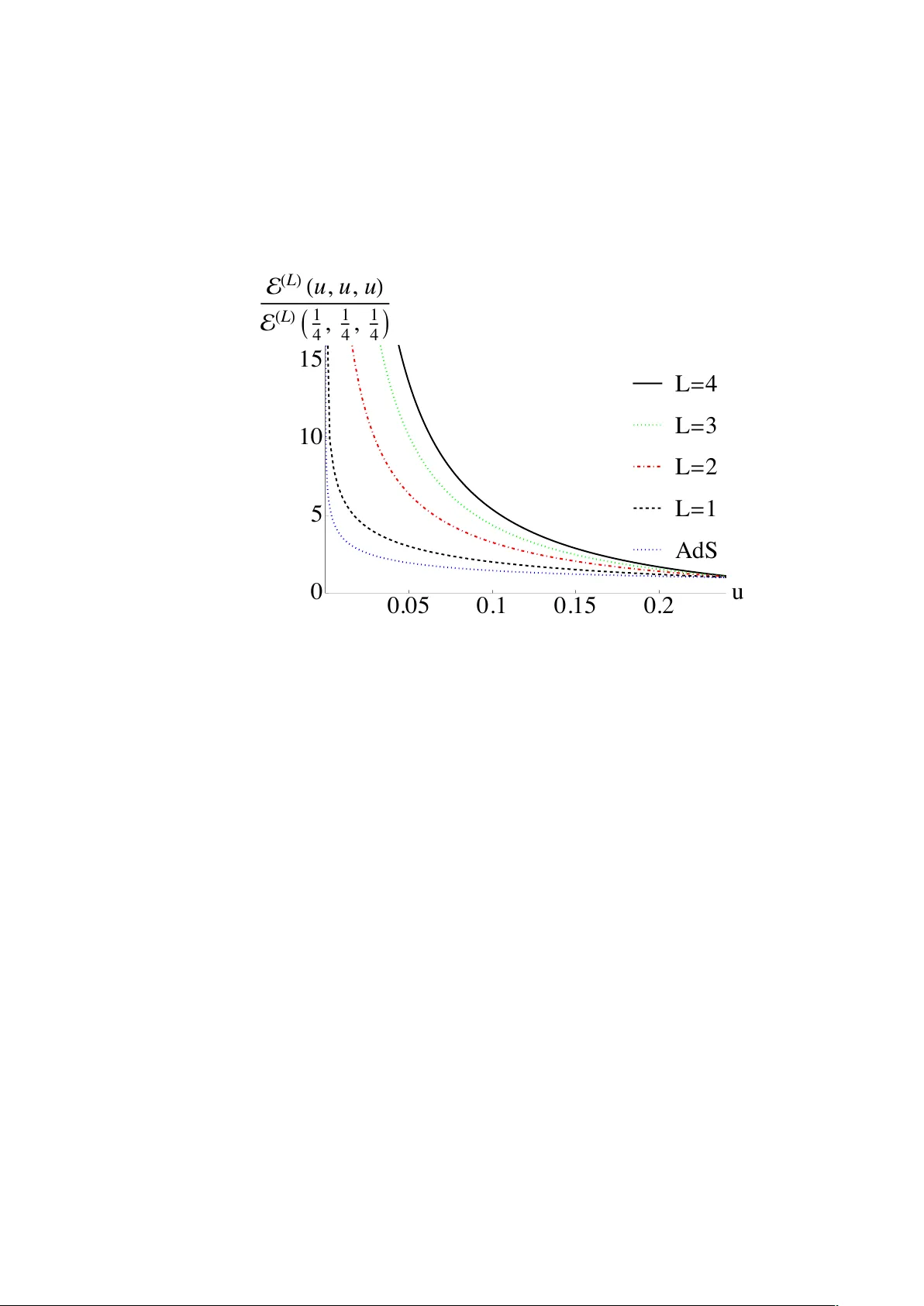
MPP-2026-59 Lecture Notes on P ositivit y Prop erties of Scattering Amplitudes Prashan th Raman a a Max-Planck-Institut f¨ ur Physik, Boltzmannstr.8, 85748 Gar ching, Germany. E-mail: praman@mpp.mpg.de Abstract W e review completely monotone (CM) and Stieltjes functions, which are classes of functions that ob ey an inﬁnite hierarc h y of p ositivit y constraints. While these are classical mathematical concepts, suc h properties ha ve recently b een sho wn to arise in man y fundamen tal building blo c ks and observ ables of quantum ﬁeld theory (QFT), such as scalar F eynman integrals in the Euclidean region and Coulomb branch amplitudes in N = 4 SYM. After reviewing their mathematical structure, w e discuss the v arious ph ysical and geometric origins of these prop erties—ranging from unitarity and analyticity in scattering amplitudes to the structure of parametric represen tations in F eynman integrals. W e then review several applications, including constrain ts on the the analytic S-matrix, implications for n umerical b o otstrap approac hes, and connections to p ositive geometries, where w e presen t evidence for a close relation b et w een these functions and geometric v olume interpretations. These lecture notes are an extended version of lectures give at the Positive Ge ometry in Sc attering Amplitudes and Cosmolo gic al Corr elators w orkshop held at the International Centre for Theoretical Sciences, Bengaluru, in F ebruary 2025. Con ten ts 1 In tro duction 3 2 Completely monotone and Stieltjes functions 4 2.1 Completely monotone functions in one v ariable . . . . . . . . . . . . . . . . . . . . . 4 2.2 Completely monotone functions in sev eral v ariables . . . . . . . . . . . . . . . . . . . 13 2.3 P olar Duals and Pro jectiv e Duality . . . . . . . . . . . . . . . . . . . . . . . . . . . . 16 2.4 Stieltjes functions in one v ariable . . . . . . . . . . . . . . . . . . . . . . . . . . . . . 19 2.5 P ad´ e approximation and conv ergence theorems . . . . . . . . . . . . . . . . . . . . . 27 3 P ositivit y prop erties of amplitudes and related observ ables 31 3.1 Completely monotone structure of the cusp anomalous dimension . . . . . . . . . . . 31 3.2 Scalar F eynman Integrals . . . . . . . . . . . . . . . . . . . . . . . . . . . . . . . . . 33 3.3 Relation b et ween disp ersion relations and p ositivit y . . . . . . . . . . . . . . . . . . 36 3.4 Coulom b branch amplitudes in N = 4 SYM . . . . . . . . . . . . . . . . . . . . . . . 38 3.5 P ositive Geometries and dual volumes . . . . . . . . . . . . . . . . . . . . . . . . . . 40 3.6 Complete monotonicity of six-particle amplitudes inside the Amplituhedron . . . . . 42 3.7 Other examples of p ositivity . . . . . . . . . . . . . . . . . . . . . . . . . . . . . . . . 43 4 Applications of p ositivit y prop erties 44 4.1 Analytic S-matrix . . . . . . . . . . . . . . . . . . . . . . . . . . . . . . . . . . . . . . 44 4.2 P ositive geometries and dual volumes . . . . . . . . . . . . . . . . . . . . . . . . . . . 46 4.3 Numerical b ootstrap applications . . . . . . . . . . . . . . . . . . . . . . . . . . . . . 52 5 Summary and Outlo ok 58 5.1 Summary . . . . . . . . . . . . . . . . . . . . . . . . . . . . . . . . . . . . . . . . . . 58 5.2 Outlo ok . . . . . . . . . . . . . . . . . . . . . . . . . . . . . . . . . . . . . . . . . . . 58 A Other p ositivit y prop erties and in tegral represen tations 60 B Momen t problem 61 B.1 Relation to completely monotone and Stieltjes functions . . . . . . . . . . . . . . . . 62 C Ab elian and T aub erian Theorems for Laplace and Stieltjes T ransforms 63 2 1 In tro duction P ositivity and conv exit y are fundamental organizing principles in quantum ﬁeld theory (QFT), often arising as consequences of basic physical requirements suc h as unitarity , causality , and analyticity . Unitarit y ensures probabilistic consistency , while analyticit y enco des causalit y and lo calit y , leading to pow erful constrain ts on ph ysical observ ables. These ideas underlie a wide range of developmen ts, including disp ersion relations, b ounds on eﬀectiv e ﬁeld theories, and the conformal b ootstrap [ 1 – 3 ]. A mo dern geometric p erspective on these structures has emerged from the study of scattering amplitudes [ 4 , 5 ]. In the framework of p ositiv e geometry , amplitudes (or their in tegrands) are iden tiﬁed with canonical diﬀerential forms asso ciated with geometric ob jects [ 5 ]. In this approac h, p ositivit y is built into the deﬁnition, and physical prop erties suc h as locality and unitarity arise as consequences of geometry [ 6 ]. In simple cases, amplitudes admit an in terpretation as v olume- lik e quan tities of dual geometric ob jects, suggesting a deep connection b et ween geometry and the analytic prop erties of QFT observ ables [ 7 ]. In perturbative QFT, observ ables are t ypically expressed as integrals where the in tegrand I is often a relatively simple rational function, while the integrated result A is a complicated tran- scenden tal function. If in tegrands are volumes then they are guaranteed to be p ositiv e in certain regions. This naturally raises the question of whether p ositivit y prop erties of the integrand surviv e in tegration, and if so, in what form [ 8 ]. Understanding this is imp ortan t b oth conceptually and practically , as suc h properties can pro vide pow erful constrain ts for analytic and numerical metho ds. Recen t w ork has shown that a remark ably strong form of positivity app ears in a wide class of fundamen tal building blocks and observ ables: complete monotonicit y [ 9 ]. This property imp oses an inﬁnite hierarch y of sign constrain ts on all deriv atives of a function and is kno wn to b e equiv alen t to the existence of a representation as a Laplace transform of a positive measure [ 10 ]. It there- fore pro vides a bridge b et ween p ositivit y , conv exit y , and in tegral represen tations. A particularly imp ortan t sub class is given by Stieltjes functions, which satisfy even stronger analytic constraints. They admit a sp ectral-t yp e represen tation with a p ositiv e measure and p ossess highly constrained analytic b eha vior in the complex plane. Strikingly , b oth completely monotone and Stieltjes structures arise naturally in QFT [ 9 , 11 ]. F or example, scalar F eynman in tegrals in the Euclidean region often fall into this class, and similar prop erties ha v e b een observed for Coulomb branch amplitudes in N = 4 SYM in suitable kinematic regimes [ 9 ]. These structures impose non-trivial constrain ts on the analytic b eha vior of ph ysical quan tities and can b e used to extract global information from limited p erturbativ e data. F rom the p ersp ectiv e of p ositiv e geometry , the app earance of these prop erties is natural due to the connection to dual v olumes. Ho w ever, the underlying reasons for their emergence can diﬀer: while in scattering amplitudes these prop erties are often consequences of unitarity and analyticity , 3 for F eynman integrals they emerge from the structural properties of parametric represen tations and Symanzik p olynomials [ 9 , 11 ]. Whenever an observ able admits a dual volume or Laplace-type represen tation ov er a p ositiv e domain, complete monotonicity follows immediately . The aim of these lecture notes is to provide a p edagogical review of these ideas. W e will study ho w general ph ysical principles lead to p ositivit y constraints, ho w these can b e strengthened to complete monotonicit y and Stieltjes properties, and ho w they are used in practice to deriv e rigorous b ounds and to b o otstrap non-trivial observ ables [ 11 ]. W e illustrate these concepts through a range of examples, highlighting b oth their physical origin and their mathematical structure. These lecture notes are based on lectures given at the Positive Ge ometry in Sc attering A m- plitudes and Cosmolo gic al Corr elators w orkshop, held at the In ternational Centre for Theoret- ical Sciences (ICTS), Bengaluru, in F ebruary 2025. A recording of the lectures is av ailable at https://www.youtube.com/live/bXsNiIOSZRs?si=1Z2GmDTFIoOU_adk . The notes are organized as follo ws. In Section 2, w e review the mathematical framew ork of completely monotone and Stieltjes functions. Section 3 surv eys examples from quantum ﬁeld theory where these p ositivit y structures arise. Section 4 discusses applications to the analytic S- matrix, p ositiv e geometry , and n umerical b o otstrap methods. The app endices provide additional bac kground on related p ositivit y classes, the moment problem, and Abelian–T aub erian theorems. 2 Completely monotone and Stieltjes functions 2.1 Completely monotone functions in one v ariable T o motiv ate the discussion that follows, consider the problem of reconstructing a function from its v alues at p ositive integers: Supp ose we are giv en a function f : R → R sp eciﬁed at all p ositive integers, f ( n ) = a n , n = 1 , 2 , 3 , . . . (1) Ho w constraining is this information? In particular: • Can we ﬁnd an in terp olating function deﬁned at all real v alues x > 0? • Under what conditions is such an interpolating function unique? • Can we construct an analytic contin uation of f to complex v alues of x ? Clearly , the function is highly undetermined: for example, b oth f ( x ) and f ( x ) + sin( π x ) satisfy the ab o ve condition. 4 A classic illuminating example is when a n = n !, in which case f ( x ) = Γ( x + 1) provides a solution. The celebrated Bohr–Mol lerup the or em states that the Gamma function is the unique solution among p ositiv e functions satisfying 1. log f ( x + 1) − log f ( x ) = log(1 + x ), ∀ x > 0, 2. Logarithmic conv exit y: log f ( x ) is conv ex i.e., (log f ( x )) ′′ ≥ 0. Let us examine these conditions more closely . The ﬁrst condition can be expressed using the forw ard diﬀerence operator ∆, ∆ f ( x ) = f ( x + 1) − f ( x ) , (2) ∆ k f ( x ) = ∆ k − 1 f ( x + 1) − ∆ k − 1 f ( x ) , k ≥ 2 , (3) so that ( − 1) k +1 ∆ k log f ( n ) ≥ 0 , ∀ k ≥ 1 , n ≥ 1 . (4) This is like a discrete deriv ative, and all suc h diﬀerences hav e ﬁxed signs. The second condition ensures smoothness and imposes a constrain t on the deriv ativ es of f ( x ): f ( x ) f ′′ ( x ) −  f ′ ( x )  2 ≥ 0 , (5) whic h is the lo g-c onvexity condition. While the Bohr–Mollerup theorem guaran tees uniqueness among p ositive functions on (0 , ∞ ), if we additionally wan t to extend the function to complex v alues, further conditions are necessary . In particular, if f is assumed to b e analytic in the right half-plane Re( x ) > 0 (as is natural for the Gamma function, whic h has p oles on the negative real axis), then Carlson ’s the or em pro vides a uniqueness result: a function that is analytic in the righ t half-plane, of exponential t yp e, and b ounded along the imaginary axis is uniquely determined by its v alues at the p ositiv e in tegers. These gro wth and analyticity constraints ensure that no “oscillatory” solutions (lik e f ( x ) + sin( π x )) can app ear in the complex extension. This example illustrates that imp osing natural constrain ts—such as p ositivit y , conv exit y , sign constrain ts on the deriv ativ es and con trolled growth—can guaran tee the uniqueness of an inter- p olating function. It also motiv ates the study of c ompletely monotone functions , which generalize these ideas to sequences and functions with higher-order sign constraints. 2.1.1 Deﬁnition and basic properties W e denote by f ( n ) ( x ) = d n dx n f ( x ) the n -th deriv ativ e of a function f . 5 Deﬁnition. A function f ∈ C ∞ ( R ) , R ⊂ R , is c al le d completely monotone (CM) if ( − 1) n f ( n ) ( x ) ≥ 0 , n ≥ 0 , ∀ x ∈ R , (6) and absolutely monotone (AM) if f ( n ) ( x ) ≥ 0 for al l n ≥ 0 and al l x ∈ R . QCD, L = 1 QCD, L = 2 QCD, L = 3 QED , L = 4 0.15 0.2 0.25 0.3 0.5 0.6 0.7 0.8 0.9 1 0.2 0.4 0.6 0.8 1.0 x 0.5 1.0 1.5 2.0 Γ cusp ( L ) ( x ) Γ cusp ∞ ( L ) Figure 1: Plot of the angle-dependent cusp anomalous dimension for QCD and QED based on a v ailable p erturbativ e data from ref [ 9 ]. As w e will see in Section 3.1 that this quantit y is exp ected to b e CM on (0 , 1). It follo ws immediately from the deﬁnition that if f is CM/AM on R = ( a, b ), then g ( x ) = f ( − x ) is resp ectiv ely AM/CM on − R = ( − b, − a ). F urthermore, if a + b < ∞ and h ( x ) = f ( a + b − x ), then h ( n ) ( x ) = ( − 1) n f ( n ) ( a + b − x ) , (7) so complete and absolute monotonicity are closely related. In the follo wing, w e fo cus exclusively on completely monotone functions. The condition in eq. (6) imp oses inﬁnitely many constraints. In particular, the cases n = 0 , 1 , 2 imply that CM functions are non-negative, monotonically decreasing, and conv ex on R . Consequen tly , CM functions and their deriv ativ es exhibit smo oth, featureless deca y , as illustrated in Fig. 1. Examples. 1. 1 x + α with α > 0, is CM on (0 , ∞ ). 6 2. β x with 0 < β < 1, is CM on (0 , ∞ ). 3. − log x is CM on (0 , 1). Basic prop erties. Using the pro duct and c hain rule for deriv ativ es, one can establish several structural properties of CM functions. W e list them here and refer to [ 12 , 13 ] for proofs. Let f , g b e CM functions on ( a, b ). 1. Con vex cone: F or λ, µ ≥ 0, the com bination λ f ( x ) + µ g ( x ) (8) is CM. Thus, CM functions form a conv ex cone. 2. Closure under pro ducts: The pro duct f ( x ) g ( x ) is CM. 3. Closure under deriv atives: F or ev ery n ∈ N , the function ( − 1) n f ( n ) ( x ) (9) is CM. 4. Closure under limits: If { f n } is a sequence of CM functions conv erging point wise to f , then f is CM. F or example, f n ( x ) = (1 − x n ) n is CM on (0 , n ) and conv erges p oin t wise to e − x as n → ∞ , whic h is therefore CM on (0 , ∞ ). 5. Comp osition (I): Let h : ( a, b ) → ( a, b ) b e a Bernstein function , i.e. h ≥ 0 and h ′ is CM. Then f ◦ h is CM on ( a, b ). In particular, if f , g are CM, then f  Z x 0 g ( t ) dt  (10) is CM (on any interv al where the argument lies in ( a, b )). 6. Comp osition (I I): Let h : ( a, b ) → R b e absolutely monotone. If f : ( a, b ) → ( a, b ) is CM, then h ◦ f is CM on ( a, b ). F or example, if log f ( x ) is CM on (0 , ∞ ), then f ( x ) = e log f ( x ) is also CM. 7 7. T runcation of the T aylor series: Using the T aylor’s reminder theorem f ( x ) = m − 1 X k =0 ( x − x 0 ) k k ! f ( k ) ( x 0 ) + Z x x 0 du ( x − u ) m − 1 ( m − 1)! f ( m ) ( u ) . (11) and noting that the CM property implies that the reminder term has ﬁxed sign. It follows that the truncation of the T aylor expansion of an y CM function f ( x ), around any p oint x = x 0 ∈ R to even and o dd order, provides a low er and upp er b ound for the function respectively i.e., 2 m X k =0 ( x − x 0 ) k k ! f ( k ) ( x 0 ) ≤ f ( x ) ≤ 2 m − 1 X k =0 ( x − x 0 ) k k ! f ( k ) ( x 0 ) for x > x 0 . (12) An imp ortant feature of completely monotone functions is their strong regularity: they are real- analytic on ( a, b ) and, in fact, admit analytic con tin uations b ey ond their domain [ 14 , 15 ]. Theorem. Bernstein ’s little the or em. If f is c ompletely monotone on ( a, b ) , then it admits an analytic c ontinuation to a disk of r adius ( b − a ) c enter e d at x = b (after suitable tr anslation of the interval). If ( a, b ) = (0 , ∞ ) then by the ab o v e result CM functions f ( z ) should admit an analytic extension to the en tire righ t half plane i.e., ℜ ( z ) > 0. This is indeed true and the Bernstein-Hausdorﬀ-Widder theorem [ 16 ] states that f is CM on (0 , ∞ ) iﬀ it is the Laplace transform of a positive function 1 . The Laplace transform in eq. (13) provides the analytic con tin uation as it conv erges for an y x = x 1 + i x 2 with x 2 ∈ R whenever x 1 > 0 and therefore con v erges in the righ t half plane. Theorem. Bernstein-Hausdorﬀ-Widder (BHW) A function f ( x ) is c ompletely monotonic on (0 , ∞ ) if and only if it admits an inte gr al r ep- r esentation f ( x ) = Z ∞ 0 dt e − xt µ ( t ) , with µ ≥ 0 . (13) The Bernstein–Hausdorﬀ–Widder (BHW) theorem pro vides a characterization of CM functions on (0 , ∞ ) and can b e used to construct non-trivial examples. F or instance, f ( x ) = log x x − 1 , with µ ( t ) = Z ∞ 0 e − ty y + 1 dy , (14) 1 The theorem is usually stated with a positive non-decreasing Borel measure dν as measures are in general allo w ed to b e distributional. This is equiv alent eq. (13) if the measure admits a well deﬁned density dν ( t ) = µ ( t ) dt with µ ( t ) ≥ 0 whic h w e hav e assumed here. 8 whic h is manifestly p ositiv e. Ho wev er, this c haracterization is not w ell-suited for testing whether a giv en function is CM, since it requires computing the inv erse Laplace transform, µ ( t ) = L − 1 ( f )( t ) = 1 2 π i Z γ + i ∞ γ − i ∞ dx e tx f ( x ) , (15) where γ ∈ R is c hosen so that the integral conv erges. This is t ypically in tractable analytically for generic functions, and while numerical in version is p ossible, certifying complete monotonicit y requires verifying µ ( t ) ≥ 0 for all t > 0. Nev ertheless, partial information about µ ( t ) can b e extracted from the asymptotic behavior of f ( x ): the b eha vior near x → ∞ and x → 0 constrains µ ( t ) near t → 0 and t → ∞ , resp ectiv ely , via T aub erian theorems (see appendix C). 2.1.2 Con v exit y properties Another important feature of completely monotone functions is that they satisfy several remark able con vexit y prop erties. These lead to non-trivial constraints on the function and its deriv ativ es, and are useful in numerical b o otstrap approac hes. These prop erties can b e view ed as successiv e strengthenings of ordinary conv exit y: from additive inequalities, to quadratic constrain ts on deriv ativ es, to m ultiplicative relations. W e summarize some of these b elo w from references [ 16 – 19 ]. A function f ( x ) is con v ex in a region R if for an y x, y ∈ R and 0 < t < 1, f ( t x + (1 − t ) y ) ≤ t f ( x ) + (1 − t ) f ( y ) . (16) CM functions ob ey a stronger generalization kno wn as the Hornich–Hla wk a prop ert y . 1. Hornic h–Hlawk a prop erty: If f ( x ) is CM on (0 , ∞ ), then for an y x 1 , . . . , x n ≥ 0, n X i =1 f ( x i ) − X i 0. F or ξ ∈ R n +1 and l ≥ 0, consider I = n X i,j =0 ( − 1) i + j + l f ( i + j + l ) ( x ) ξ i ξ j . (20) Using f ( x ) = R ∞ 0 e − xt µ ( t ) dt , w e obtain I = Z ∞ 0 dt µ ( t ) e − xt t l n X i =0 t i ξ i ! 2 ≥ 0 . (21) Th us, the quadratic form is non-negative, and hence the asso ciated matrix is positive semidef- inite. Cho osing l = 0 , 1 yields the result. This provides a reﬁnemen t of con vexit y at the level of deriv atives: instead of constraining f itself, we demand p ositivit y of quadratic forms built from its higher deriv atives. Con versely , p ositivit y of these Hank el matrices implies the non-negativity of all signed deriv a- tiv es ( − 1) n f ( n ) ( x ), since their diagonal entries are non-negative. T ogether with regularit y conditions, this provides a characterization of complete monotonicity [ 16 ]. This yields an inﬁnite set of quadratic constrain ts on deriv ativ es. F or instance,      f ( x ) − f ′ ( x ) − f ′ ( x ) f ′′ ( x )      ≥ 0 (22) implies the lo g-c onvexity condition w e sa w in eq. (5) with higher-order constrain ts arising from larger determinants. 3. Sc hur con v exity: Let m 1 ≥ · · · ≥ m n b e non-negative integers. Deﬁne u x ( m 1 , . . . , m n ) = ( − 1) m 1 f ( m 1 ) ( x ) · · · ( − 1) m n f ( m n ) ( x ) . (23) Then u x ( m 1 , . . . , m n ) is monotone under redistribution of the m i that preserv es their sum 10 and ordering in the sense that k X i =1 m i ≤ k X i =1 m ′ i for all k = 1 , . . . , n − 1 , (24) and n X i =1 m i = n X i =1 m ′ i = ⇒ u x ( m 1 , . . . , m n ) ≤ u x ( m ′ 1 , . . . , m ′ n ) . (25) This can b e viewed as a m ultiplicative strengthening of con vexit y: instead of linear or quadratic combinations, one considers ordered redistributions of deriv ative indices, and de- mands monotonicity under ma jorization. Some examples (see [ 13 ]): (a) F or m = (1 , 1 , 1) and m ′ = (2 , 1 , 0), Sch ur conv exit y implies  f ′ ( x )  3 ≥ f ′′ ( x ) f ( x ) . (26) This inequalit y do es not follow from Hank el matrix p ositivity , and illustrates that Sch ur con vexit y imp oses constraints b eyond those captured b y Hank el determinants. (b) F or any integers k , j ≥ 0, the function x 7→     f ( k + j ) ( x ) f ( k ) ( x )     (27) is decreasing. In summary , these prop erties form a hierarc hy of increasingly strong constrain ts: Hornich–Hla wk a enco des global additiv e inequalities generalizing conv exit y; Hank el matrix p ositivit y reﬁnes this to quadratic constraints on deriv atives (including log-con vexit y); and Sc hur con vexit y further imp oses higher-order multiplicativ e inequalities that are not captured by ﬁnite Hank el conditions. 2.1.3 In terp olation of sequences via completely monotone functions Let us now return to the question p osed at the b eginning of this section and see how CM functions can b e used to solve the interpolation problem in eq. (1). A useful result in this context is the follo wing: Theorem (M ¨ un tz theorem for CM functions, [ 20 ]) . L et ( a n ) n ∈ N b e a strictly incr e asing se quenc e 11 of p ositive numb ers, 0 < a 1 < a 2 < . . . , with lim k →∞ a k → ∞ such that ∞ X n =1 1 a n = ∞ . (28) Supp ose f and g ar e c ompletely monotone functions on (0 , ∞ ) satisfying f ( a n ) = g ( a n ) , ∀ n ∈ N . (29) Then f ( x ) = g ( x ) , ∀ x ∈ (0 , ∞ ) . (30) In other words, if you kno w a CM function on (0 , ∞ ) on a set of p oints that don’t thin out to o quic kly , then it is uniquely determined. In particular, if w e ﬁnd a CM function with prescrib ed v alues at the positive integers, then it is unique. Rather remark ably , if such a function exists, it can b e constructed explicitly using the Newton series: Theorem (Theorem 3.1 in [ 21 ]) . L et I ⊂ R b e a right-unb ounde d op en interval, and let f : I → R b e inﬁnitely diﬀer entiable. Supp ose that for some q ∈ N , the derivative f ( q ) ( x ) is c ompletely monotone on I . Then, for any a ∈ I , f admits the Newton series exp ansion f ( x ) = ∞ X k =0  x − a k  ∆ k f ( a ) , x ∈ I , (31) and the series c onver ges uniformly on c omp act subsets of I . The ab o ve theorem shows that it is suﬃcient for some deriv ative of the function to b e CM. This explains, for instance, wh y the Bohr–Mollerup c haracterization w orks: even though f ( x ) = log Γ(1 + x ) is not CM, one of its deriv atives, the trigamma function, f ′′ ( z ) = Z ∞ 0 dt t e − t 1 − e − t e − tz , (32) is CM. Using eq. (31) with a = 1 and f ( n ) = log( n − 1)! for n = 1 , 2 , . . . , w e obtain the Newton series f ( z ) = ∞ X n =1  z n  n X k =1 ( − 1) n − k  n − 1 k − 1  log k , ℜ ( z ) > 0 , (33) whic h is kno wn as the Stern series for the log-gamma function. 12 W e can rep eat this construction for other sequences. F or example, consider a n = 1 x 0 + n , x 0 > 0 , (34) whic h is obtained b y sampling the function f ( x ) = 1 /x at x = x 0 + n , n ∈ N 0 . The Newton series then yields 1 x = 1 x 0 ∞ X k =0 ( − 1) k  x − x 0 k   x 0 + k k  , ℜ ( x ) > 0 . (35) In summary , if w e are given a sequence { a n } n ≥ 0 whic h arises as the v alues of a function whose deriv atives ev en tually b ecome completely monotone on (0 , ∞ ), then the Newton series in eq. (31) pro vides an explicit interpolation of this sequence to a function deﬁned on the righ t half-plane. In physics language, the Newton series plays a role analogous to a disp ersion relation, recon- structing the full function from discrete data together with p ositivity constraints. This construction gives a constructiv e and analytic answer to the initial interpolation problem: not only is the function uniquely determined under suitable CM conditions, but it can also b e explicitly written and analytically con tin ued to ℜ ( x ) > 0. 2.2 Completely monotone functions in several v ariables W e will no w lo ok at the class of CM functions in several v ariables and on more general domains that are needed for applications in physics. A function f : R n → R is completely monotone in I ⊆ R n if it satisﬁes ( − ∂ x 1 ) m 1 . . . ( − ∂ x n ) m n f ( x 1 , . . . , x n ) ≥ 0 , ∀ m i ∈ Z ≥ 0 and ∀ ( x 1 , ..., x n ) ∈ I (36) whic h is just a straightforw ard generalization of the single v ariable deﬁnition in eq.(6). Examples. 1. A linear function with non-negative co eﬃcien ts raised to a negative p o w er, f ( x 1 , . . . , x n ) = 1 ( c 1 x 1 + . . . c n x n + d ) α , ∀ c i ≥ 0 , α , d ≥ 0 . (37) This follo ws directly from the deﬁnition in eq. (36). This example though very simple is very imp ortan t for many applications such as to F eynman integrals as we shall see in section 3.2. 13 The case of non-linear polynomials raised to negative p o w ers is more complicated and in volv es h yp erb olic p olynomials [ 22 , 23 ] see the discussion around 4.2. 2. A simple 2 v ariable example is f ( x 1 , x 2 ) = 1 x 1 − x 2 log  b + x 1 b + x 2  (38) whic h is CM on R 2 + for b ≥ 0 whic h can b e seen by f ( x 1 , x 2 ) = Z R 2 + du dv e − b ( u + v ) u + v e − u x − v y (39) 3. As a t wo-v ariable example inv olving polylogarithms, the follo wing function app ears in a ﬁnite sev en-p oin t one-lo op integral [ 24 ], Ψ (1) ( x 1 , x 2 ) = Li 2 (1 − x 1 ) + Li 2 (1 − x 2 ) + log x 1 log x 2 − π 2 / 6 . (40) whic h is CM in the region x 1 + x 2 ≤ 1. T o see that this is CM, it is useful to consider g ( x 1 , x 2 ) = Ψ (1) ( x 1 , x 2 ) 1 − x 1 − x 2 , (41) whic h has the disp ersiv e integral representation, g ( x 1 , x 2 ) = Z ∞ 0 Z ∞ 0 dy 1 dy 2 ( x 1 + y 1 )( x 2 + y 2 )(1+ y 1 + y 2 ) . (42) F rom this equation it is manifest that g is CM on R 2 + . Moreo ver, in view of eq. (41), we can deduce that Ψ (1) is CM, in the region x 1 + x 2 ≤ 1. Multiv ariate completely monotone functions in pro jectiv e space are c haracterized by a generaliza- tion of the Bernstein–Hausdorﬀ–Widder theorem due to Cho quet [ 25 ]. T o state this result, we ﬁrst clarify the notion of complete monotonicity on cones. 2.2.1 Completely monotone functions on pro jectiv e space Let V b e a ﬁnite-dimensional vector space. A c one is a subset C ⊂ V such that C = λx | x ∈ C , ; λ > 0 , . (43) 14 The dual c one is deﬁned as C ∗ = y ∈ V ∗ | ⟨ y , x ⟩ ≥ 0; ; ∀ x ∈ C , , (44) where ⟨ y , x ⟩ = P i x i y i . Deﬁnition. A function f : C → R is c ompletely monotone (CM) if ( − 1) k D v 1 · · · D v k f ( x ) ≥ 0 , , ∀ v 1 , . . . , v k ∈ C, ∀ x ∈ C, k = 0 , 1 , 2 , . . . (45) wher e D v denotes the dir e ctional derivative along v . T o c hec k complete monotonicity of a function f ( x ) on a con vex cone C ⊂ R n , one m ust in principle v erify eq. (45) for arbitrary directions v i ∈ C . In practice, it is suﬃcient to chec k these deriv ativ es along the extr emal r ays of the cone. Deﬁnition (Extremal ray) . A r ay R = { λ v | λ ≥ 0 } is c al le d an extr emal r ay if it c annot b e written as a non-trivial sum of two ve ctors in C . That is, if v = u 1 + u 2 with u 1 , u 2 ∈ C , then u 1 and u 2 must b e pr op ortional to v with non-ne gative c o eﬃcients. The complexity of v erifying CM prop erties dep ends on whether the cone is p olyhe dr al or non- p olyhe dr al . A cone is p olyhe dr al if it is generated b y ﬁnitely many extremal rays v 1 , . . . , v m . 1. (The p ositive orthant). The simplest case is C = R n + . The extremal rays are the basis v ectors e i = (0 , ... 1 , ..., 0). Checking CM reduces to v erifying ( − 1) k ∂ ∗ i 1 · · · ∂ i k f ≥ 0. 2. (A simplex c one). Consider C = { ( x, y ) | 0 < x < y } , with extremal rays v 1 = (0 , 1) and v 2 = (1 , 1). F or the function f ( x, y ) = y x ( y − x ) , (46) one ﬁnds ( − 1) n D n v 1 f = n ! ( y − x ) n , ( − 1) n D n v 2 f = n ! x n , D v 1 D v 2 f = 0 , (47) sho wing that f is CM on C . A cone is non-p olyhe dr al if it requires inﬁnitely man y extremal rays. 15 1. (The L or entz/light c one). In 2 + 1 dimensions, C = ( t, x, y ) | t ≥ p x 2 + y 2 (48) has a contin uous family of extremal ra ys. “‘ Consider f ( x, y ) = 1 1 − x 2 − y 2 , x 2 + y 2 < 1 . (49) This homogenizes to ˆ f ( x, y , z ) = 1 z 2 − x 2 − y 2 (50) on the cone C = { ( x, y , z ) | z ≥ 0 , z 2 − x 2 − y 2 ≥ 0 } . (51) F or a generic direction v = ( r cos θ , r sin θ , z ) with z > r , one ﬁnds − D v ˆ f = 2 z 2 − r 2 ≥ 0 , (52) and more generally ( − 1) k D v 1 · · · D v k ˆ f = Y i 1 z 2 − r 2 i ≥ 0 , (53) sho wing that f is CM on C . 2. (Positive semideﬁnite c one). The cone of symmetric p ositiv e semideﬁnite matrices S n + is non-p olyhedral for n ≥ 2. Its extremal rays corresp ond to rank-one matrices v v T . 2.3 P olar Duals and Pro jective Dualit y Let A ⊂ R m +1 b e a conv ex b o dy containing the origin in its in terior. Deﬁnition. (Polar dual:) The p olar dual of A is the set A ∗ = { W ∈ ( R m +1 ) ∗ | W · Y ≥ − 1 ∀ Y ∈ A } . (54) After pro jectivization, one often writes A ∗ = { W | W · Y ≥ 0 ∀ Y ∈ A } , (55) dep ending on normalization conv en tions. This is the conv en tion we adopt in the follo wing examples. 16 Geometrically , the p olar dual A ∗ is the set of hyperplanes that do not intersect the in terior of A , and the b oundary of A ∗ corresp onds to hyperplanes tangent to A . Dualit y is inv olutiv e up to closure: ( A ∗ ) ∗ = A for suﬃciently regular conv ex b o dies. T o construct the p olar dual explicitly , w e pro ceed in t w o steps: 1. T angency condition: A dual vector W lies on the b oundary of A ∗ if it is normal to a tangen t hyperplane of A . F or a diﬀeren tiable b oundary , this gives W = λ ∇ f ( Y ) , (56) where f ( Y ) = 0 deﬁnes the b oundary of A . 2. Dualit y (normalization) condition: The hyperplane deﬁned b y W must satisfy W · Y = − 1 , (57) whic h ﬁxes the scale factor λ . Examples: 1. Circle: F or the unit circle f ( x, y ) = x 2 + y 2 − 1 = 0, the tangency condition gives u = 2 λx, v = 2 λy , and the duality condition u x + v y = − 1 yields λ = − 1 / 2. Substituting bac k, w e ﬁnd the dual curve u 2 + v 2 = 1 , sho wing the circle is self-dual. 2. Cubic: F or f ( x, y ) = x 3 + y 3 − 1 = 0, the tangency condition gives u = 3 λx 2 , v = 3 λy 2 , and u x + v y = 1 determines λ . Eliminating ( x, y , λ ) gives the dual cubic 1 − 2 u 3 − 2 v 3 − 2 u 3 v 3 + u 6 + v 6 = 0 . 3. n -Sphere: F or the unit n -sphere f ( x 1 , . . . , x n ) = P n i =1 x 2 i − 1 = 0, tangency gives W = 2 λ ( x 1 , . . . , x n ) , 17 and the duality condition W · ( x 1 , . . . , x n ) = − 1 implies λ = − 1 / 2. Substituting bac k yields n X i =1 W 2 i = 1 , sho wing that the unit n -sphere is self-dual. The p olar dual enco des all supp orting hyp erplanes of a con vex b o dy . One can think of the supp ort function h A ( W ) = sup Y ∈ A W · Y as measuring the maximal ”shadow” of A in the direction W . The dual A ∗ consists of all W for whic h this shado w is b ounded b y a c hosen normalization. This construction is closely related to the Legendre transform : f ∗ ( W ) = sup Y  W · Y − f ( Y )  , whic h exc hanges v ariables for their conjugate momenta. In classical mec hanics, this is exactly the step from the Lagrangian to the Hamiltonian: the dual v ariables W pla y the role of momen ta, arising from the tangency and dualit y conditions, just like velocities are replaced by momenta via a Legendre transform. Completely monotone functions on cones are characterized b y the follo wing in tegral represen- tation. Theorem ( Bernstein–Hausdorﬀ–Widder–Cho quet). A function f on an op en c one C ⊂ R n is c ompletely monotone if and only if it admits the r epr esentation f ( x ) = Z C ∗ e −⟨ y ,x ⟩ , dµ ( y ) , , (58) wher e µ is a p ositive me asur e supp orte d on the dual c one C ∗ . In particular if C = R n + , then C ∗ = C and this reduces to the standard m ultidimensional Laplace transform with a positive measure. The BHWC theorem admits a natural geometric interpretation in pro jective space. F or example, for µ ( y ) ≡ 1 in eq. (58): I ( x ) = Z C ∗ e −⟨ y ,x ⟩ d n +1 y . (59) 18 Using the homogeneity of the cone, one can perform the radial integral: I ( x ) = Z C ∗ 1 ⟨ y , x ⟩ n d n y , (60) whic h can b e in terpreted as a pro jectiv e in tegral ov er the dual cone.The resulting “volume” dep ends on the choice of x , whic h selects an aﬃne slice of the dual cone, b ut diﬀeren t c hoices of x corresp ond to equiv alen t pro jectiv e measures. More generally , allowing a non-negative measure µ ( y ) ≥ 0 promotes this to a w eighted, or “generalized”, pro jective volume. Ev ery completely monotone function on a conv ex cone can b e represen ted as an in tegral ov er the dual cone. In pro jectiv e terms, this means that eac h CM function secretly encodes a (p ossibly weigh ted) pro jective v olume of the dual cone. This as we shall see explains why such functions are natural when we talk ab out dual volumes and p ositiv e geometries. W e will see more ab out this connection in section 2. When a m ultiv ariate rational function is completely monotone on a conv ex cone, this property is in timately related to the notion of h yp erbolic p olynomials [ 22 ], [ 23 ],[ 26 ]. W e will end this section b y reviewing this connection 2.4 Stieltjes functions in one v ariable Till now, w e hav e studied functions with a r e al pr op erty : complete monotonicity . While this prop ert y indirectly implies analyticity in certain strips of the complex plane, it remains quite restrictiv e. Many functions of interest in ph ysics are inheren tly complex-v alued and exhibit richer analytic structure. W e now turn our atten tion to a sp ecial sub class of completely monotone functions, known as Stieltjes functions . These functions are particularly w ell-b eha ved: they are analytic in the cut complex plane C \ ( −∞ , 0] and satisfy a complex-analytic property called the Her glotz pr op erty . Stieltjes functions ob ey analogues of unsubtracted disp ersion relations and are remark ably amenable to rational appro ximation tec hniques, suc h as P ad´ e appro ximations. Remark ably , using only the T a ylor expansion of a Stieltjes function on the positive real axis, one can accurately appro ximate its v alues anywhere in the cut complex plane. In this sense, Stieltjes functions generalize the idea of analytically contin uing a completely monotone function to the en tire righ t half-plane via the Newton series, using only its v alues at the p ositive in tegers. With this motiv ation in mind, we no w turn to a formal deﬁnition of Stieltjes functions and summarize their key prop erties. 19 2.4.1 Deﬁn tion and basic prop erties Deﬁnition. A function f ( z ) analytic in the cut plane C \ ( −∞ , − R ] is c al le d a Stieltjes function if it admits an inte gr al r epr esentation f ( z ) = Z 1 /R 0 ρ ( u ) 1 + u z du , with ρ ( u ) ≥ 0 ∀ u ∈ (0 , 1 /R ) . (61) It follo ws from eq. (61) that Stieltjes functions form a subset of completely monotonic (CM) functions, since ( − ∂ z ) n f ( z ) = Z 1 /R 0 du u n n ! ρ ( u ) (1 + uz ) n +1 ≥ 0 . (62) Remark. In the literature, one also commonly deﬁnes a Stieltjes function b y the representation f ( z ) = Z 1 /R 0 ρ ( u ) z + u du . (63) The form (61) used here is more natural for P ad´ e approximation applications. The t w o represen- tations are equiv alen t and can b e mapp ed into each other by a simple change of v ariables. Examples 1. Rational example: f ( z ) = 1 1 + z = Z 1 0 du δ ( u − 1) 1 1 + uz . (64) 2. Logarithmic example: f ( z ) = log(1 + z ) z = Z 1 0 du 1 + uz . (65) 3. Polylogarithms: Li n +1 ( − z ) − z = Z 1 0 dt ( − log t ) n 1 + z t . (66) In principle, the measure ρ ( u ) can b e recov ered from f ( z ) via the inv ersion formula ρ ( u ) = Disc f ( − 1 /u ) − u , Disc f ( x ) = lim ϵ → 0 ( f ( x + iϵ ) − f ( x − iϵ )) , (67) but in practice this in version is cumbersome. This motiv ates alternative c haracterizations. Widder pro vided a real-v ariable deriv ativ e criterion similar to eq. (6) for completely monotone functions, 20 Theorem. ( Widder’s r e al variable char eterization) A r e al-value d function deﬁne d on (0 , ∞ ) is Stieltjes if and only if ( − 1) n ( x k f ( x )) ( n + k ) ≥ 0 ∀ n, k ≥ 0 , x > 0 . (68) When k = 0, this reduces to the conditions deﬁning CM functions. Stieltjes functions require additional p ositivit y conditions on deriv ativ es, which ensures that they can b e analytically con- tin ued to the full cut plane C \ ( −∞ , 0], whereas CM functions generally extend only to the righ t half-plane. W e hav e eq. (61) which is lik e the Laplace transform characterization of completely monotone functions on (0 , ∞ ) namely eq. (13) . And w e hav e Widder’s condition eq. (68) on the deriv ativ es b eing p ositiv e analogous to eq.(6) for CM functions. While these conditions are elegant, they are not alw ays practical for veriﬁcation. More con ve- nien t characterizations are complex-analytic in nature. F ollo wing ref. [ 27 , Sec. 8.6], it is suﬃcient to verify the following prop erties to prov e a function is Stieltjes: 1. Analyticity: f ( z ) is analytic in the cut complex plane C \ ( −∞ , − R ]. 2. Asymptotic b ehavior: f ( z ) → C ≥ 0 as | z | → ∞ . 3. Her glotz pr op erty: − f ( z ) is Herglotz, i.e. ℑ f ( z ) ℑ z < 0 ∀ z / ∈ R . (69) These conditions imply the Stieltjes representation (61) as follo ws. Consider the function f ( w ) − C w , where the subtraction ensures the in tegrand decays as | w | − 2 at inﬁnit y . Applying Cauc h y’s theorem on a keyhole contour around the cut ( −∞ , − R ] w e get f ( z ) − C = 1 2 π i Z − R −∞ Disc f ( x ) x − z dx, Disc f ( x ) = lim ϵ → 0 ( f ( x + iϵ ) − f ( x − iϵ )) . The Herglotz prop ert y guarantees ℑ f ( x + i 0) ≤ 0, allowing us to deﬁne the positive measure ρ ( u ) = − 1 π u ℑ f  − 1 u + i 0  , u ∈ (0 , 1 /R ) , 21 and changing v ariables x = − 1 /u yields f ( z ) = C + Z 1 /R 0 ρ ( u ) 1 + u z du, whic h is exactly the Stieltjes represen tation. The constan t C can b e absorb ed into the measure if desired. So in summary condition 1 allows us to apply Cauch y’s theorem in the cut plane, condition 2 tells us w e need at most one subtractions to make the function decay for large argumen t and condition 3 ensures that the discon tin uity across the branc h cut is p ositiv e and together they imply Stieltjes functions as subtracted dispersion relations A Stieltjes function is precisely a function that admits a once-subtracted disp ersion relation with a p ositiv e discontin uit y across the branch cut. This observ ation explains wh y suc h functions naturally arise in man y ph ysical applications. An alternative version is due to Krein’s Theorem (Krein’s characterization) . A function f : (0 , ∞ ) → R is Stieltjes if and only if f ( x ) ≥ 0 for x > 0 , and f admits an analytic c ontinuation to C \ ( −∞ , 0] such that ℑ f ( z ) ≤ 0 whenever ℑ z ≥ 0 . Th us, these conditions pro vide a direct analytic route to pro ving that a function is Stieltjes, without the need for inv erting measures explicitly or c hecking inﬁnitely many inequalities are satisﬁed. The key ingredient in these c haracterizations is the Herglotz prop ert y , whose consequences w e no w brieﬂy discuss. The Herglotz prop ert y ℑ f ( z ) ℑ z < 0 ∀ z / ∈ R (70) means that f maps the upp er and lo wer half-planes to opp osite half-planes. Despite the appar- en t simplicity of this condition, it imp oses strong constrain ts on the analytic structure of f . In particular: 1. All p oles and zeros of f lie on the real axis. 2. All p oles and zeros are simple, with p oles having p ositiv e residues. 22 T o see this, consider the lo cal b eha vior of f ( z ) near a singularit y or zero z = z 0 : f ( z ) ∼ A ( z − z 0 ) γ , (71) where γ ∈ R . W riting ( z − z 0 ) = r e iθ and A = A 0 e iϕ with A 0 , r > 0, we obtain ℑ f ( z ) ∼ A 0 r γ sin( γ θ + ϕ ) . (72) F or z approaching z 0 from the upp er half-plane, θ ∈ (0 , π ). The Herglotz property requires ℑ f ( z ) < 0 throughout this interv al, so the function sin( γ θ + ϕ ) cannot change sign. This is only possible if the total v ariation of the argument is at most π , which implies | γ | ≤ 1 . F or meromorphic functions, γ ∈ Z \ { 0 } , hence γ = ± 1, sho wing that all p oles and zeros are simple. F or a p ole ( γ = − 1), we require sin( ϕ − θ ) < 0 for all θ ∈ (0 , π ). T aking limits: • θ → 0 + giv es sin( ϕ ) ≤ 0, • θ → π − giv es sin( ϕ − π ) ≤ 0, i.e. sin( ϕ ) ≥ 0. Th us sin( ϕ ) = 0, and the inequalit y ﬁxes ϕ = 0, so A = A 0 > 0. Hence all p oles hav e p ositiv e real residues. F or a zero ( γ = 1), the condition sin( θ + ϕ ) < 0 for all θ ∈ (0 , π ) forces ϕ = π , so A = − A 0 . Summary . T o v erify that a function is Stieltjes, it suﬃces in practice to chec k that: • f ( x ) ≥ 0 for x > 0, • f satisﬁes the Herglotz property . These constraints immediately exclude certain completely monotone functions. F or example, f ( x ) = 1 (1 + x ) 2 is completely monotone but not Stieltjes, as it has a double p ole, which is forbidden. Similarly , f ( x ) = 1 x 3 + x is completely monotone on (0 , ∞ ) but not Stieltjes, since it has p oles oﬀ the real axis. W e end this discussion b y p ointing out that unlik e CM functions Stieltjes functions are not closed under 23 deriv ativ es or pro ducts as the ab o v e examples clearly show. The main reason for this is the tension with the Herglotz prop ert y . Nonetheless w e now metion a re lated class of functions which one w ould get if we take deriv ativ es of a Stieltjes function. 2.4.2 Generalized Stieltjes F unctions A natural extension of the space of Stieltjes functions, denoted S λ , is deﬁned b y the following in tegral representation (cf. ref. [ 28 ]): f ( z ) = Z 1 /R 0 ρ ( u ) (1 + u z ) λ du, with ρ ( u ) ≥ 0 , λ > 0 . (73) When λ = 1, we recov er the standard Stieltjes class. Key Prop erties • Geometric Mapping (The W edge Prop ert y): While a standard Stieltjes function maps the upp er half-plane (UHP) to the low er half-plane (LHP), a GSF of order λ maps the UHP to a sp eciﬁc we dge . F or z ∈ UHP, the phase of the function is constrained b y: − min( π , π λ ) < arg f ( z ) < 0 . (74) F or λ < 1, the image is a narro w wedge of angle π λ within the LHP . F or λ > 1, the image co vers the entire LHP and can extend onto further Riemann sheets. • (Nested Inclusivit y): The classes S λ satisfy a nested inclusion property . If α < β , then: S α ⊂ S β . (75) This implies that any standard Stieltjes function ( λ = 1) is automatically a generalized Stieltjes function of order λ for all λ > 1. • Con version to Standard Stieltjes F orm: A GSF of order λ > 1 can b e mappe d back to the standard S 1 class through a p ow er transformation of the co ordinate. Speciﬁcally , if f ( z ) ∈ S λ , then: g ( z ) = f ( z 1 /λ ) = ⇒ g ( z ) ∈ S 1 . (76) Lik e we alluded to earlier pro duct of Stieltjes functions is not Stieltjes, w e now list what prop- erties preserve the prop ert y . 24 2.4.3 Closure Prop erties The deﬁnition of Stieltjes functions through the Herglotz mapping and the intgeral represen ta- tion leads to a remark ably rigid set of algebraic prop erties. Man y of these follo w from Krein’s c haracterization [ 29 ]: Let f ( z ) , g ( z ) b e Stieltjes functions. Then: 1. Con vex cone: F or any λ, µ > 0, λf ( x ) + µg ( x ) is Stieltjes. Why: The sum of tw o measures dµ 1 + dµ 2 remains a p ositiv e measure, and the LHP- mapping prop ert y is preserved under linear com binations with p ositiv e co eﬃcien ts. 2. Closure under P o wers: F or 0 ≤ α ≤ 1, h ( x ) = f ( x ) α is Stieltjes. Why: If arg f ∈ ( − π , 0), then arg f α ∈ ( − π α, 0). F or α ≤ 1, this range is con tained within ( − π , 0), main taining the Anti-Herglotz prop ert y . 3. Closure under H¨ older pro ducts: F or 0 ≤ α ≤ 1, h ( x ) = f ( x ) α g ( x ) 1 − α is Stieltjes. Why: The phase of the product is the conv ex com bination of the phases: arg h = α arg f + (1 − α ) arg g . Since both phases are in ( − π , 0), their weigh ted av erage is also in ( − π , 0). 4. In version and Scaling: • h ( x ) = 1 f (1 /x ) is Stieltjes. • h ( x ) = 1 xf ( x ) is Stieltjes. • F or λ > 0, f ( x ) λf ( x )+1 is Stieltjes. Why: These transformations eﬀec tiv ely swap the LHP and UHP or inv ert the v ariable z . F or example, 1 /z maps the UHP to the LHP , and the homographic transform is a conformal map that preserves the half-plane geometry . 5. Comp osition: f ◦ 1 g and 1 f ◦ g are Stieltjes. Why: The inner function 1 /g maps the UHP to the UHP; the outer function f then maps that UHP to the LHP , satisfying the Stieltjes condition. 6. Closure under limits: If { f n ( x ) } is a sequence of Stieltjes functions conv erging p oin twise, lim n →∞ f n ( x ) is Stieltjes. 25 Why: The set of p ositiv e measures is closed under w eak conv ergence, ensuring the limit maintains a v alid sp ectral representation. 7. M¨ obius T ransformations: g ( z ) = 1 cz + d f  az + b cz + d  for a, b, c, d ≥ 0 and ad − bc > 0 is Stieltjes. Substituting the integral representation f ( z ) = R µ ( t ) 1+ z t dt into g ( z ) yields: g ( u ) = Z 1 /R 0 µ ( t ) ( bt + d )  1 + u at + c bt + d  dt. (77) By deﬁning the change of v ariables y = at + c bt + d , we get: g ( u ) = Z a + cR b + dR c/d 1 1 + u y  µ ( t ( y )) a − b y  | {z } ν ( y ) dy . (78) Since a, b, c, d ≥ 0 and ad − bc > 0, the mapping t 7→ y is monotonic and a − by > 0 on the supp ort. Th us, ν ( y ) ≥ 0, and g ( u ) is conﬁrmed to be a Stieltjes function. Note that the fractional linear transformation g ( z ) = 1 cz + d f ( az + b cz + d ) is distinct from the comp osition prop ert y f ◦ (1 /g ). While comp osition inv olv es nesting tw o Stieltjes functions, the FL T represents a symmetry of the Stieltjes class itself. The pre-factor ( cz + d ) − 1 is essential. If we expand the integral representation eq. (61) around z → 0 w e get f ( z ) ∼ ∞ X n =0 ( − 1) n a n z n , a n > 0 , (79) where the co eﬃcien ts are giv en b y the moments of the measure, a n = Z 1 /R 0 u n ρ ( u ) du. (80) When R > 0, the in tegration range is ﬁnite and all momen ts exist. Ho wev er, for R = 0 the integral extends to inﬁnity , and the momen ts need not exist. In this case, the expansion around z = 0 may in volv e logarithmic terms rather than a pure pow er series. In practice, this issue can be av oided b y expanding around an y p oin t z 0 > 0. Indeed, the shifted function g ( z ) = f ( z + z 0 ) (81) 26 is again Stieltjes b y prop ert y 7 with a = 1 , b = z 0 , c = 0 , d = 1 , and takes R 7→ R + z 0 > 0. This ensure the existence of a moment expansion of the form eq. (79) Example. The function f ( z ) = log z z − 1 = Z ∞ 0 du (1 + z u )(1 + u ) (82) do es not admit ﬁnite moments at z = 0. Ho wev er, g ( z ) = f (1 + z ) = log(1 + z ) z = Z 1 0 du 1 + z u (83) do es. The existence of moment expansions, together with the positivity and con trolled analytic struc- ture of Stieltjes functions, mak es them particularly well-suited for rational approximation. These features lead to p ow erful conv ergence results for P ad ´ e approximan ts, to which we now turn. 2.5 P ad´ e appro ximation and conv ergence theorems The Pad ´ e approximation (P A) is a simple and useful alternative to p olynomial approximations of analytic functions. Supp ose we are given the T a ylor expansion of a function f ( z ) ab out a p oint x 0 , f ( z ) = ∞ X k =0 a k ( z − x 0 ) k , (84) whic h conv erges in some neigh b orhoo d of x 0 . T o construct the Pad ´ e appro ximant, one proceeds as follo ws: • T runcate the T aylor series to K = N + M + 1 terms. • Find a rational function P N M ( z ; x 0 ) = A 0 + A 1 ( z − x 0 ) + · · · + A N ( z − x 0 ) N 1 + B 1 ( z − x 0 ) + · · · + B M ( z − x 0 ) M , (85) suc h that its T aylor expansion agrees with that of f ( z ) up to order N + M + 1. Th us, the P ad ´ e approximan t pro vides a rational approximation to the analytic function f ( z ). It has tw o k ey adv antages: • Analytic c ontinuation: It allo ws one to ev aluate the function outside the radius of conv ergence of the original T aylor series. 27 • Series ac c eler ation: It often conv erges m uc h faster than the T aylor series within its domain of conv ergence. P ad´ e appro ximations can b e applied to any function but in particular the mathematical theory is v ery w ell dev elop ed and understo od for Stieltjes functions. In particular, for Stieltjes functions analytic in C \ ( −∞ , − R ], Pad ´ e appro ximants satisfy the following remark able prop erties: (a) Conver genc e on the r e al axis. F or x ∈ R \ ( −∞ , − R ] with x ≥ x 0 : – The sequence { P N N ( x ; x 0 ) } is monotonically decreasing in N . – The sequence { P N − 1 N ( x ; x 0 ) } is monotonically increasing in N . – These sequences b ound the function: P N − 1 N ( x ; x 0 ) ≤ f ( x ) ≤ P N N ( x ; x 0 ) , x ≥ x 0 . (86) (b) Poles and r esidues. F or J ≥ − 1, the Pad ´ e approximan ts P N + J N ( z ; x 0 ) hav e only simple p oles lo cated on ( −∞ , − R ) with p ositive residues. In particular, P N − 1 N ( z ; x 0 ) = N X i =1 β i 1 + γ i z , β i , γ i ≥ 0 . (87) (c) Conver genc e in the cut plane. In C \ ( −∞ , − R ], the sequences { P N N ( z ; x 0 ) } and { P N − 1 N ( z ; x 0 ) } con verge to f ( z ), pro vided the coeﬃcients of the asymptotic expansion satisfy | a n | = O ((2 n )! C n ) (88) for some constant C . (d) Err or b ounds. Let ∆ > 0 and deﬁne D + (∆) = { x + iy ∈ C | x ≤ − R, | y | ≥ ∆ } ∪ { x + iy ∈ C | x > − R } . (89) If the asymptotic expansion of f ( z ) is conv ergen t, then for z ∈ D + (∆), | f ( z ) − P M + J M ( z ; x 0 ) | < c     z − x 0 ρ     J +1     √ ρ + z − x 0 − √ ρ √ ρ + z − x 0 + √ ρ     2 M , (90) for all J ≥ − 1, M ≥ 1, where ρ = R + x 0 − ∆ and c is a constant. Th us, Pad ´ e appro ximants pro vide conv ergen t rational approximations to Stieltjes functions on the real axis and in the cut complex plane, with controlled analytic structure and rigorous error b ounds. 28 2.5.1 Multiv ariate Stieltjes functions Similar to univ ariate case, inthe multiv ariate case also there are tw o closely related in tegral repre- sen tations of Stieltjes functions,though these seem to not b e ob viously equiv alen t. Let f ( z 1 , . . . , z n ) b e analytic in ( C \ ( −∞ , 0]) n . Then f is considered a multiv ariate Stieltjes function if it admits either of the following forms: • V ersion 1 (CM functions with a CM measure p ersp ectiv e): f ( z 1 , . . . , z n ) = Z ∞ 0 . . . Z ∞ 0 dt 1 . . . dt n µ ( t 1 , . . . , t n ) ( t 1 + z 1 ) . . . ( t n + z n ) , (91) with µ ( t 1 , . . . , t n ) ≥ 0. This is a direct generalization of univ ariate CM/Stieltjes functions to m ultiple v ariables. Each v ariable z i en ters via a separate CM k ernel. • V ersion 2 (m ultiv ariate P ad ´ e p ersp ectiv e): f ( z 1 , . . . , z n ) = Z ∞ 0 . . . Z ∞ 0 dt 1 . . . dt n µ ( t 1 , . . . , t n ) 1 + t 1 z 1 + · · · + t n z n . (92) V ersion 2 is particularly natural when constructing m ultiv ariate P ad´ e appro ximan ts, as the denominator is linear in each v ariable, whic h preserves monotonicity and p ositivit y prop erties necessary for conv ergence results analogous to the univ ariate case [ 30 ]. A concrete example arises in N = 4 SYM theory . Consider the six-particle MHV remain- der/ratio function, or equiv alently , the four-p oin t in-in correlator of a conformally coupled scalar exc hange on a de Sitter bac kground: f ( u, v ) = Li 2 (1 − u ) + Li 2 (1 − v ) + log u log v − ζ 2 1 − u − v . (93) This function can b e written in both V ersion 1 and V ersion 2 forms: V ersion 1: f ( u, v ) = Z R 2 + dx dy 1 ( x + u )( y + v )(1 + x + y ) , (94) V ersion 2: f ( u, v ) = Z R 2 + dx dy 1 (1 + x )(1 + y )(1 + xu + y v ) , (95) where the second representation is obtained by a change of v ariables x → xu , y → y u . Ho wev er, not all m ultiv ariate functions are Stieltjes in b oth represen tations. F or instance, the 29 Mandelstam representation of the one-lo op Coulomb branch amplitude in N = 4 SYM [ 31 ], f 1 ( u, v ) = Z 1 0 dx Z 1 − x 0 dy 1 ( x + u )( y + v ) √ 1 − x − y , (96) ﬁts manifestly only in to V ersion 1. Understanding which represen tation is appropriate in general remains an op en question for more complicated multiv ariate integrals. 30 3 P ositivit y prop erties of amplitudes and related observ ables W e now review sev eral examples of building blo c ks like F eynman integrals and observ ables suc h as amplitudes in quan tum ﬁeld theory that exhibit the positivity properties discussed abov e. These examples were iden tiﬁed in ref. [ 9 ], and we limit ourselves here to a brief review of a few of them, referring the reader to the original reference for other examples and more details. Broadly sp eaking, the origin of these p ositivit y prop erties can b e traced to three distinct mech- anisms: 1. Represen tation-theoretic argumen ts: Positivit y follo ws from explicit in tegral represen- tations with manifestly p ositiv e kernels or can b e argued for directly from the explicit result. 2. Analyticit y and causality: General prop erties of the S-matrix, suc h as analyticit y , unitar- it y , and crossing symmetry , lead to disp ersion relations and in-turn positivity . 3. P ositive geometry: In N = 4 SYM, observ ables admit geometric in terpretations and p osi- tivit y is expected from suc h considerations. 3.1 Completely monotone structure of the cusp anomalous dimension A prominent example where complete monotonicit y arises in quantum ﬁeld theory is the angle- dep endent cusp anomalous dimension . Consider a Wilson line containing a cusp with op ening angle ϕ . Its exp ectation v alue exhibits an ultraviolet divergence of the form ⟨ W cusp ⟩ ∼ 1 ϵ Γ cusp ( ϕ ) , (97) where Γ cusp ( ϕ ) go verns infrared singularities of scattering amplitudes [ 32 ], anomalous dimensions of large-spin op erators [ 33 , 34 ], and the quark–antiquark p oten tial [ 35 ]. If v ariable x = e iϕ and w e restrict to the Euclidean region x ∈ (0 , 1) then the cusp anomalous dimension admits a p erturbative expansion of the form Γ cusp ( x ) = X L ≥ 1 g 2 L Γ ( L ) cusp ( x ) . (98) 31 Figure 2: Wilson line containing a cusp with op ening angle ϕ . The result from ref. [ 9 ] is: Complete monotonicity of the angle dep enden t cusp anomalous dimension. The angle-dep endent cusp anomalous dimension ( − 1) L +1 Γ ( L ) cusp ( x ) (99) is a completely monotone function in x ∈ (0 , 1). This has b een chec k ed based on av ailable p erturbative data up to L = 3 in QCD and N = 4 SYM, and up to L = 4 in QED. As a simple illustration, the one-lo op result is given by Γ (1) cusp ( x ) = 1 − x 1 + x ( − log x ) , (100) whic h is manifestly completely monotone on (0 , 1), since all 3 factors 1 − x , 1 1+ x and − log x are all CM on (0 , 1) and the property is preserved when w e take pro ducts. Has b een chec k ed in planar N = 4 SYM upto 3 lo ops [ 36 ] but also QCD at three lo ops [ 37 ] and in QED at four loops [ 38 ]. In the Euclidean region x ∈ (0 , 1), the cusp anomalous dimension diverges logarithmically as x → 0, Γ cusp ( x ) ∼ − Γ ∞ cusp log x, (101) while it v anishes at x = 1. If one rescales the functions to match their small- x asymptotics, their shap es b ecome remark ably similar across diﬀeren t theories (see Fig. 1), despite diﬀering n umerically at the level of a few p ercen t. 32 3.2 Scalar F eynman Integrals Scalar F eynman in tegrals are the basic building blo c ks of the amplitudes in QFT. They are given b y F eynman parametrization (see ref [ 39 ]) for a giv en F eynman graph G with L lo ops in D dimensions and take the form I ( x i ) = Γ  P i ν i − LD 2  Q i Γ( ν i ) Z α i ≥ 0 Y i dα i δ  1 − X i α i  α ν i − 1 i U ( α ) P i ν i − ( L +1) D 2 F ( α i , x i ) P i ν i − LD 2 . (102) Where U and F are Graph polynomials deﬁned b y U ( α ) = X T ∈T 1 Y e i / ∈ T α i , (103) F ( { α i } , { x i } ) = X ( T ,R ) ∈T 2   Y e i / ∈ ( T ,R ) α i   ( − s T ,R ) + U ( α ) n X i =1 α i m 2 i . (104) where T 1 and T 2 are spanning trees and tw o-forests resp ectiv ely . The kinematical v ariables are giv en by s ( T ,R ) =  X e i / ∈ ( T ,R ) q i  2 (105) { x i } = {− s ( T ; R ) , m 2 i } . (106) The Euclidean region is deﬁned as E = {{ x i } | F ( { α i } ; { x i } ) ≥ 0 ∀ α i ≥ 0 } . (107) F or example, for the massiv e bubble integral, we hav e F ( α 1 , α 2 ; s, m 2 ) = α 1 α 2 ( − s ) + m 2 ( α 1 + α 2 ) 2 (108) and demanding eq.(107) gives: E ( s, m ) = { ( s, m ) | s ≤ 4 m 2 } . (109) Another example is the massiv e b o x integral with equal in ternal mass. Here we hav e F ( α 1 , ..., α 4 ; s, t, m 2 ) = α 1 α 3 ( − s ) + α 2 α 4 ( − t ) + ( α 1 + α 2 + α 3 + α 4 ) 2 m 2 (110) 33 and eq. (107) gives E ( s, t, m 2 ) = { ( s, t, m ) | s ≤ 4 m 2 , t ≤ 4 m 2 } . (111) The Euclidean region admits a natural geometric in terpretation as a c op ositive c one , see ref. [ 40 ]. Within this region, scalar F eynman in tegrals exhibit remark able p ositivit y properties. In ref. [ 9 ], it w as shown that scalar F eynman integrals are completely monotone (CM), and subsequently in ref. [ 11 ] that, under suitable conditions, they are in fact Stieltjes functions. The origin of these prop erties can b e traced back to the F eynman parameter represen tation in eq. (102). There, the dep endence on the kinematic v ariables x i en ters exclusively through the second Symanzik p olynomial F ( x i , α i ), which is linear in the x i and app ears raised to a negative p o w er. Since functions of this type are completely monotone (and, under stronger conditions, Stieltjes), it follows that the full F eynman in tegral inherits these prop erties, pro vided the in tegral con verges. Indeed, p ositive linear combinations preserve b oth complete monotonicity and the Stieltjes prop ert y . There are, how ev er, tw o imp ortan t subtleties: 1. The kinematic v ariables x i are not all indep enden t, and one m ust therefore c ho ose a set of indep enden t v ariables b efore establishing complete monotonicit y . 2. F or sp ecial kinematic conﬁgurations, the Euclidean region itself ma y b e empty , obstructing the applicability of these arguments. These issues do not arise for planar integrals, but they can o ccur in the non-planar case. In suc h situations, an additional technical condition on the second Symanzik p olynomial is required. A simple example illustrating these subtleties is pro vided by massless four-particle scattering. In this case, the Mandelstam v ariables s, t, u satisfy s + t + u = 0, so that the v ariables y = {− s, − t, − u } cannot all be p ositiv e sim ultaneously . As a result, the Euclidean region is empt y , and the second Symanzik p olynomial need not b e p ositiv e deﬁnite, as happ ens for instance in the non-planar double b o x in tegral. Moreov er, all three v ariables enter non-trivially in F , making it imp ossible to isolate an indep enden t p ositiv e set. This situation changes if one of the external legs is taken oﬀ-shell. F or example, if p 2 4  = 0, then the relation becomes s + t + u = p 2 4 , and the Euclidean region is non-empty . In this case, one can trade u for s, t, p 2 4 , which form an indep enden t set of v ariables, allo wing the previous arguments to go through. 34 3 L+1 3 L 3 L-1 4 1 2 3 1 2 3 4 5 6 2 L-1 2 L+1 Figure 3: Some families of F eynman in tegrals that are Stieltjes (a) Banana in tegrals in D = 2 (b) b o x intgerals in D = 6 (c) zig-zag integrals in D = 4. W e can now summarize the results of refs. [ 9 , 11 ]. Suﬃcien t condition for scalar F eynman in tegrals to b e completely monotone functions Theorem ( see [ 9 ],[ 11 ]) . Sc alar F eynman inte gr als, as deﬁne d in e q. (102), ar e c ompletely monotone functions in the variables x i in the Euclide an r e gion if the se c ond Symanzik p oly- nomial c an b e written in the form F = X i A i x i , (112) with A i ≥ 0 . F or planar F eynman inte gr als this c ondition is satisﬁe d gener al ly and we c an cho ose { x i } = {− s T ,R , m 2 i } . F or non-planar inte gr als, ther e is str ong evidenc e fr om explicit examples that the ab ove c ondition on the Symanzik p olynomial c ontinues to hold, although a gener al pr o of r emains an op en pr oblem. W e hav e used the multi-v ariate version of complete monotonicity eq.(36). How ev er for the Stieltjes we stic k to the single v ariate version with the understanding that all other v ariables are held ﬁxed in the Euclidean region. 35 Suﬃcien t condition for scalar F eynman in tegrals to b e Stieltjes functions Theorem (see ref. [ 11 ]) . Sc alar F eynman inte gr als, as deﬁne d in e q. (102), ar e Stieltjes functions pr ovide d the fol lowing c onditions ar e satisﬁe d. (i) The pr op agator p owers and kinematic p ar ameters ob ey 0 < X i ν i − LD 2 ≤ 1 , (113) wher e L is the lo op or der, D the sp ac etime dimension, and ν i the pr op agator exp onents. (ii) The se c ond Symanzik p olynomial c an b e written in the form F = A x + B , (114) with A ≥ 0 and B ≥ 0 . Under these assumptions, the inte gr al deﬁnes a Stieltjes function of the variable x when al l the other variables ar e held ﬁxe d in the Euclide an r e gion. F or planar F eynman inte gr als, this c ondition is satisﬁe d quite gener al ly: the variable x may b e taken to b e any kinematic invariant of the form x = − ( p i + p i +1 + · · · + p j − 1 ) 2 or x = m 2 i , (115) with al l other variables held ﬁxe d in the Euclide an r e gion. F or non-planar inte gr als, ther e is str ong evidenc e fr om explicit examples that the ab ove c on- dition on the Symanzik p olynomial c ontinues to hold, although a gener al pr o of r emains an op en pr oblem. As we review in section 4.3 these p ositivit y prop erties can b e used to numerically constrain F eynman integrals. Remark ably these properties allo w us to constrain F eynman in tegrals not just in the Euclidean region but also in Loren tzian kinematics. 3.3 Relation b et w een disp ersion relations and positivity In certain cases the existence of a disp ersion relation and unitarity can imply p ositivity prop er- ties. In these cases we can imagine that the p ositivit y prop erties are a non-trivial consequence of unitarit y , causality/analyticit y of the S-matrix. 36 Consider a function A ( s ) that satisﬁes an unsubtr acte d disp ersion relation A ( s ) = Z ∞ 4 m 2 ds ′ Disc A ( s ′ ) s ′ − s (116) By p erforming a v ariable transformation to the Euclidean region x = − s , and using the Sch winger tric k 1 x + s ′ = Z ∞ 0 dt e − t ( x + s ′ ) (117) w e can rewrite the amplitude as a Laplace transform: A ( x ) = Z ∞ 0 dt e − tx Z ∞ 4 m 2 ds ′ e − ts ′ Disc A ( s ′ ) | {z } µ ( t ) (118) This represen tation allows us to classify the amplitude based on the nature of its sp ectral density: • Stieltjes Prop ert y: If Disc A ( s ′ ) ≥ 0, then A ( x ) is a Stieltjes function. This is a stronger condition that can typically follow from Unitarit y and the Optical Theorem. • Complete Monotonicity (CM): If µ ( t ) ≥ 0, then A ( x ) is a CM function for x > 0. 3.3.1 Spectral Represen tation of V acuum P olarization The v acuum p olarization function Π( q 2 ) can be described using the K¨ al l´ en-L ehmann sp e ctr al r ep- r esentation , whic h relates the full propagator to a sp ectral density ρ ( s ). F or gauge-inv ariant ob- serv ables, the spectral density ρ ( s ) is guaranteed to be positive-deﬁnite for all s ≥ s thr , i.e., ab ov e the threshold for particle pro duction. This p ositivit y is a direct consequence of the unitarity of the theory . T o ensure the photon remains massless (Π(0) = 0) and to render the in tegral ultraviolet ﬁnite, one usually employs a once-subtracted disp ersion relation : Π( q 2 ) = q 2 Z ∞ s thr ρ ( s ) s ( s − q 2 ) ds (119) By changing of v ariables u = 1 /s and Q 2 = − q 2 > 0, we get Π( Q 2 ) = − Q 2 Z 1 /s thr 0 ρ (1 /u ) 1 + u Q 2 du (120) Stieltjes prop ert y of the v accum p olarization If Π( Q 2 ) is the v accum p olarization function then − Π( Q 2 ) Q 2 is a Stieltjes function. 37 0.2 0.4 0.6 0.8 1.0 ξ 0.2 0.4 0.6 0.8 1.0 η ∫ Δ ρ ( ξ , η ) e - p ξ - q η  ξ  η positive ρ ( ξ , η ) positive Figure 4: Regions inside the in tegration domain ∆ where eq.(113),(114) hold fot L = 2. 3.4 Coulom b branc h amplitudes in N = 4 SYM The Coulomb branc h amplitudes [ 41 ], which depend on the kinematic v ariables u = 4 m 2 / ( − s ) , v = 4 m 2 / ( − t ). P ositivity prop erties of Coulomb branch amplitudes ( − 1) L M ( L ) ( u, v ) is a CM function of u, v , for u > 0 , v > 0 using the av ailable results [ 31 ] at L = 1 , 2 , 3. F or L = 1 , −M (1) ( u, v ) is also a Stieltjes function. The 4-p oin t amplitudes on the Coulom b branch admit a remark ably simple Mandelstam repre- sen tation [ 31 ]: M ( u, v ) = Z ∆ dξ dη ρ ( ξ , η ) ( ξ + u )( η + v ) (121) where ∆ is the integration region ∆ = { ξ , η ≥ 0 , ξ + η ≤ 1 } . Just lik e in the previous section b y using Sch winger’s trick eq. (117) the b eha vior of the double sp ectral function ρ ( ξ , η ) determines the mathematical class to whic h of the amplitude: • Stieltjes: The amplitude is Stieltjes if ρ ( ξ , η ) ≥ 0 . (122) • Completely monotone: The amplitude is CM for u, v > 0 if the following in tegral holds for all p, q ≥ 0: Z ∆ dξ dη ρ ( ξ , η ) e − ξ p − ηq ≥ 0 (123) F or L = 1 eq. (122) holds but for L = 2 only the w eaker condition eq. (123) holds as sho wn 38 in the ﬁgure 4 . L = 4 L = 3 L = 2 L = 1 AdS 0.05 0.1 0.15 0.2 u 0 5 10 15 ℰ ( L ) ( u , u , u ) ℰ ( L )  1 4 , 1 4 , 1 4  Figure 5: Beha vior of E ( L ) ( u, u, u ) in the region 0 < u < 1 / 4. F rom b ottom to top: strong coupling and L = 1 , 2 , 3 , 4 lo op results. The curves are p ositiv e, monotonically decreasing, and conv ex, as exp ected for completely monotone functions. In ref. [ 42 ], the authors numerically b o otstrap the four-point Coulom b branc h amplitude in N = 4 SYM using S-matrix b o otstrap techniques. The functional space is constrained by dual conformal inv ariance, while the numerical inputs are anchored b y integrabilit y-deriv ed data and exact Regge tra jectories across all coupling strengths. Remark ably , they ﬁnd evidence that c omplete monotonicity (CM) p ersists at ﬁnite coupling. This result is particularly striking given that in the same ref. [ 42 ] it w as demonstrated that the ﬁnite-coupling amplitude cannot satisfy a standard Mandelstam represen tation. T ypically , CM is a consequence of the simple spectral properties associated with such represen tations, its p ersistence in their absence suggests that the positivity of the amplitude is go v erned b y a deeper, p erhaps more fundamen tal, geometric principle that transcends the traditional analytic structure of p erturbativ e QFT. W e will no w discuss the connection to p ositiv e geometries which is indeed suc h a formulation of QFT. 39 3.5 P ositiv e Geometries and dual v olumes The p ositive ge ometry pr o gr am asso ciates certain physical theories with a p ositive ge ometry and directly computes scattering amplitudes from its structure [ 4 , 5 , 43 ]. Remark ably , in this framework, fundamen tal prop erties suc h as lo calit y and unitarit y emerge rather than being imp osed. T ree-level amplitudes and lo op-lev el integrands are encoded as diﬀer ential forms on the positive geometry . Examples: • All lo ops, all multiplicities: planar N = 4 SYM, ϕ 3 theory , ABJM theory . • Up to one loop, all m ultiplicities: scalar theories with colour. A D -dimensional p ositive geometry is a space carved out b y a system of homogeneous poly- nomial equations and inequalities, with b oundaries of all co-dimensions, and a unique associated meromorphic D -form, called the c anonic al form [ 5 ]. Every b oundary comp onen t is itself a p ositiv e geometry of low er dimension, and taking the residue of the canonical form at a b oundary gives the canonical form of that boundary . A t tree level, amplitudes can b e interpreted as the volume of a dual p olytop e [ 7 ]. A t lo op level, this interpretation is conjectural: the dual amplituhe dr on is not y et kno wn [ 8 ]. While we do not y et kno w if the integrands do correspond to dual volumes they seem to b e p ositiv e inside the geometry . In tegrating these forms produces scattering amplitudes, and while the p ositivit y of the in tegrated results is non-trivial, empirical evidence supp orts it [ 44 ]. F ollo wing the framew ork of p ositiv e geometries (cf. ref. [ 5 ]), we can understand the origin of complete monotonicity as a consequence of the analytic structure of canonical forms. Deﬁnitions and the Residue Prop erty A p ositive ge ometry is a pair ( X , X ≥ 0 ) where X is a complex pro jectiv e v ariet y and X ≥ 0 is a closed subset of the real part X ( R ). It is equipped with a unique meromorphic d -form Ω( X, X ≥ 0 ) called the c anonic al form , uniquely determined by the prop ert y that it has simple p oles only on the b oundaries of X ≥ 0 , and its residues are recursively deﬁned: Res F Ω( X , X ≥ 0 ) = Ω( F , F ≥ 0 ) (124) where F is a b oundary comp onen t (facet) of X ≥ 0 . F or a 0-dimensional p oint, Ω(pt) = ± 1. 40 Examples 1. The Interv al: Consider the interv al in X = P 1 ( R ) with X ≥ 0 = { (1 , x ) ∈ P 1 ( R ) | a ≤ x ≤ b } . The canonical form is the unique 1-form with simple p oles at a and b with unit residues: Ω([ a, b ]) =  1 x − a − 1 x − b  dx = b − a ( x − a )( x − b ) dx. (125) 2. The T riangle: Consider a triangle T in X = P 2 ( R ) with X ≥ 0 = { (1 , x, y ) | y ≥ 0 , 1 − x − y ≥ 0 , 1 + x − y ≥ 0 } . The canonical form tak es the form: Ω( T ) = N dx ∧ dy y (1 − x − y ) (1 + x − y ) (126) T aking residues we see, Res y =0 ,x =1 = N 2 Res y =0 ,x = − 1 = N 2 Res y =1 ,x =0 = − N 2 (127) all of these hav e to b e ± 1 so w e get N = 2. 3. The Half-Pizza (Non-Polytopal Geometry) : Another example is half-pizza geometry , whic h includes a non-linear b oundary . It is deﬁned b y the region: P = { (1 , x, y ) | y + 1 2 ≥ 0 , 1 − x 2 − y 2 ≥ 0 } (128) The canonical form for this region is: Ω P = √ 3 dx ∧ dy ( y + 1 2 ) (1 − x 2 − y 2 ) (129) Dual Laplace Represen tation and Complete Monotonicit y Consider the case of conv ex p olytopes A ∈ P m ( R ) in pro jectiv e space, whic h in simple cases describ e scattering amplitudes [ 7 ]. The canonical rational function Ω( Y ) = Ω( Y ) ⟨ Y d m Y ⟩ of suc h a polytop e is the volume of the dual polytop e A ∗ Y . The latter is deﬁned b y the facet inequalities W · Y > 0, for Y ∈ A and for any W ∈ A ∗ Y . The canonical function admits the follo wing Laplace represen tation 41 [ 5 ], Ω( Y ) = 1 m ! Z W ∈ A ∗ Y e − W · Y d m +1 W . (130) This prov es that Ω( Y ) is CM for any Y ∈ A by Cho quet’s theorem eq. 58, with measure µ = 1. According to this theorem, the directional deriv ativ es are to be tak en along the extremal rays of the dual p olytop e A ∗ Y . Canonical rational function of an y con vex p olytop e is completely monotone The canonical rational function Ω( Y ) of an y conv ex polytop e A ∈ P m ( R ) for any Y ∈ A is completely monotone. This fact suggests to us a close connection b et ween the CM prop ert y and dual geometries. This could help when lo oking for a dual geometry in cases b ey ond p olytop es, such as the conjectured dual Amplituhedron [ 45 – 47 ]. 3.6 Complete monotonicit y of six-particle amplitudes inside the Amplituhedron An imp ortan t motiv ation for studying positivity prop erties of in tegrated observ ables comes from p ositiv e geometry . In planar N = 4 sup er Y ang–Mills theory , scattering amplitudes are asso ciated with geometric ob jects known as Amplituhedra. A t the lev el of lo op integrands, these ob jects lead to rational functions that are conjectured to admit a geometric (v olume) interpretation and are manifestly p ositiv e inside the corresponding region [ 4 , 7 , 45 ]. A natural question is whether such p ositivit y prop erties p ersist after in tegration ov er lo op momen ta. Evidence for this w as found in [ 8 ], where it was observ ed that suitably deﬁned ﬁnite parts of integrated amplitudes remain positive when ev aluated on kinematic conﬁgurations inside the tree-level Amplituhedron. A particularly well-studied example is the six-particle amplitude after infrared subtraction. Using the BDS-lik e normalization [ 48 – 50 ], one obtains a ﬁnite, dual-conformally in v arian t function E ( u, v , w ) dep ending on three cross ratios. The relev an t kinematic domain is the tree-lev el MHV Amplituhedron region P MHV : u > 0 , v > 0 , w > 0 , u + v + w < 1 , ( u + v + w − 1) 2 < 4 uv w . (131) W e expand E perturbatively in the coupling, E ( u, v , w ) = X L ≥ 1 g 2 L E ( L ) ( u, v , w ) . (132) 42 Complete monotonicity in the Amplituhedron F or planar N = 4 sup er Y ang–Mills theory , consider the six-particle amplitude E ( u, v , w ) in the BDS-lik e normalization. Then, for kinematic v ariables ( u, v , w ) inside the tree-lev el MHV Amplituhedron region P MHV , the p erturbativ e co eﬃcients satisfy ( − 1) L E ( L ) ( u, v , w ) is completely monotone in ( u, v , w ) . (133) This prop ert y has b een prov en analytically at one and tw o lo ops, is supp orted by strong n umerical evidence at three and four lo ops, and is consistent with the strong-coupling result. A t lo w lo op orders, this statemen t can be established rigorously . Complete monotonicity has b een pro ven analytically for L = 1 and L = 2, using explicit represen tations of the amplitude in terms of p olylogarithmic functions and F eynman in tegrals. A t higher lo op orders, Strong numerical evidence supports the v alidit y of complete monotonicity at L = 3 and L = 4 throughout the Amplituhedron region. By restricting to the symmetric slice u = v = w , where the kinematic domain reduces to 0 < u < 1 / 4. On this slice, the strong-coupling result derived from AdS/CFT can b e sho wn to satisfy complete monotonicity as w ell. This pro vides a non-p erturbativ e consistency c hec k of the conjectured structure. The qualitativ e b eha vior displa yed in Fig. 5 is c haracteristic of completely monotone functions: the functions are p ositiv e, decreasing, and con vex throughout the domain. Remark ably , this simple pattern emerges despite the highly non-trivial analytic structure of the underlying amplitudes, whic h inv olv e iterated integrals of increasing transcendental w eight. This example provides strong evidence that p ositivit y prop erties inherited from the Amplituhedron extend b ey ond the lev el of in tegrands and persist, in a highly non-trivial w a y , after integration. 3.7 Other examples of p ositivit y W e ﬁnally mention that in ref. [ 9 ] and subsequently evidence for complete monotonicit y has been found for several other ob jects including Wilson lo ops with a Lagrangian insertions [ 51 , 52 ], cos- mological correlators [ 53 ], energy correlators [ 54 ] and string amplitudes [ 9 ]. While our entire review has b een ab out studying p ositivit y prop erties in the kinematics, a natural question to ask w ould be if such prop erties can also b e seen in the coupling. This w as in vestigated for sev eral exact observ ables in 4 dimensional sup er Y ang Mills theories in ref. [ 55 ] and strong evidence and in some cases proofs were found that several of these observ ables satisfy b oth complete monotoncity and Stieltjes prop erties in the coupling. 43 4 Applications of p ositivit y prop erties Ha ving review ed both the mathematical framew ork for Stieltjes and completely monotone functions and v arious examples where such prop erties arise in physics. W e no w lo ok at some applications of these ideas. W e will primarily follo w refs. [ 11 , 26 ] 4.1 Analytic S-matrix 4.1.1 Martin p ositivit y b ounds W e now discuss an application of p ositivit y prop erties in constraining the S-matrix and deriving rigorous non-p erturbativ e b ounds. W e follow the discussion of [ 56 ]. Consider the 2 → 2 scattering amplitude M ( s, t, u ) of iden tical massiv e scalar particles of mass m . Under general ph ysical assumptions—unitarit y , analyticit y , crossing symmetry , and p olyno- mial b oundedness (e.g. the F roissart–Martin bound)—the amplitude satisﬁes a ﬁxed- t disp ersion relation. In particular, for − t 0 ≤ t ≤ 4 m 2 , one can write a twice-subtracted disp ersion relation M ( s, t ) = c ( t ) + 1 π Z ∞ 4 m 2 ds ′  s 2 s ′ 2 ( s ′ − s ) + u 2 s ′ 2 ( s ′ − u )  A ( s ′ , t ) , (134) where A ( s ′ , t ) = Im M ( s ′ , t ) and u = 4 m 2 − s − t . Unitarit y implies positivity of the absorptiv e part, A ( s ′ , t ) > 0 , s ′ ≥ 4 m 2 , 0 ≤ t ≤ 4 m 2 . (135) The Mandelstam triangle (the region s, t, u < 4 m 2 ) corresp onds to an unphysical region where the amplitude is real and constrained b y crossing symmetry (see Figure 6). Its vertices lie at s = 4 m 2 , t = 4 m 2 , u = 4 m 2 , while its edges corresp ond to s = 0, t = 0, u = 0. The symmetric p oin t P 0 = 4 m 2 3 (1 , 1 , 1) (136) is inv ariant under p erm utations of ( s, t, u ). 44 Figure 6: The Madelstram triangle for equal mass 2-2 sacttering. The coloured regions indicate where exactly one of the inequalities eq. (137)-(138) are v alid. It can b e shown [ 56 ] that inside the Mandelstam triangle the amplitude satisﬁes the inﬁnite set of p ositivit y conditions, for all n ≥ 0, d n ds n M ( s, t ) > 0 for ﬁxed t, 2 m 2 − t 2 ≤ s ≤ 4 m 2 , (137) d n dt n M ( s, t ) > 0 for ﬁxed s, 2 m 2 − s 2 ≤ t ≤ 4 m 2 , (138) d n dt n M (4 m 2 − u − t, t, u ) > 0 for ﬁxed u, 2 m 2 − u 2 ≤ t ≤ 4 m 2 . (139) Up to a c hoice of conv en tions (in [ 56 ] one uses ( s, t, u ) ↔ ( − s, − t, − u )), these inequalities imply that the amplitude exhibits completely monotone b eha vior along each kinematic direction inside the Mandelstam triangle. These constrain ts lead to strong global prop erties of the amplitude. In particular, M ( s, t, u ) attains its minimum at the crossing-symmetric p oin t, M ( s, t, u ) ≥ M  4 m 2 3 , 4 m 2 3 , 4 m 2 3  . (140) W e no w giv e an intuitiv e argument for this fact. The Mandelstam triangle can be partitioned in to three regions, in eac h of whic h one of the inequalities (137)–(139) con trols the v ariation of the amplitude. Mo ving inw ard from any v ertex to ward the in terior, the ﬁrst-deriv ativ e p ositivit y ( n = 1) implies that the amplitude decreases along these directions. The second-deriv ative condition 45 ( n = 2) enforces conv exit y , and together with crossing symmetry ensures that the symmetric p oint P 0 is the unique global minim um. This provides a rigorous, non-p erturbativ e lo wer b ound for any scattering amplitude ob eying (134). F rom the p ersp ectiv e of this work, this result can be understo o d as a direct consequence of the (directional) complete monotonicity of the amplitude inside the Mandelstam triangle. In fact, [ 56 ] further uses these p ositivit y prop erties to derive bounds on partial w a ves as w ell as absolute n umerical b ounds, for example 0 ≤ M  4 3 , 4 3 , 4 3  < M (2 , 2 , 0) < 3 . 6 for m 2 = 1 . (141) 4.2 P ositiv e geometries and dual v olumes Let us now return to the question p osed at the end of section 3.5, namely whether complete monotonicit y can be used to construct duals of non-p olytopal p ositiv e geometries. As a ﬁrst example, consider the cone o v er the half-pizza geometry deﬁned in eq. (128), given b y the region (see Fig. 7a) P = { ( z , x, y ) | y + z 2 ≥ 0 , z 2 − x 2 − y 2 ≥ 0 } . (142) Its canonical form is Ω P = √ 3 dx ∧ dy ∧ dz ( y + z 2 )( z 2 − x 2 − y 2 ) . (143) Using the construction of section (2.3), the dual region is found to decomp ose as P ∗ = P 1 ∪ P 2 , (144) where P 1 = { ( w , u, v ) | w ≥ 0 , w 2 − u 2 − v 2 ≥ 0 } , (145) P 2 = { ( w , u, v ) | w ≥ 0 , | u | ≤ √ 3 2 w , p 1 − u 2 ≤ v ≤ 2 − √ 3 | u |} . (146) W e no w attempt to repro duce the canonical function via a Laplace transform, as in the p olytop e case. Deﬁning Ω P = √ 3 ( y + z 2 )( z 2 − x 2 − y 2 ) , w e compute Z P ∗ du dv dw e − xu − y v − z w = Ω P + Ω T , (147) 46 (a) The half-pizza P (b) The dual half-pizza P ∗ where Ω T is a transcendental contribution inv olving logarithms. Th us, unlik e the p olytop e case, the naive dual v olume do es not repro duce the canonical function. If Ω P admits an interpretation as a dual volume, this suggests t w o p ossibilities: • either P ∗ is not the correct notion of dual geometry , and the duality must b e mo diﬁed. • or P ∗ is the correct dual, but the measure m ust b e generalized to a non-trivial density µ ( u, v , w ). W e can tak e inspiration from Bernstien–Hausdorﬀ-Widder–Choquet theorem eq. (58) that the latter is p ossible. In ref. [ 26 ] we explored ho w to construct the non-trivial measures building on the works [ 22 , 23 ]. The question w e just p osed can b e formalized with the notion of a Completely monotone positiv e geometry deﬁned in [ 26 ]. Deﬁnition (Completely monotone p ositiv e geometry) . We c al l a pr oje ctive c onvex p ositive ge om- etry ( P m , P ) c ompletely monotone if the c anonic al function Ω b P is c ompletely monotone on b P , up to an over al l choic e of sign. It was already well known that rational functions whic h are completely monotone ha v e a close relation with the notion of h yp erb olic p olynomials see refs. [ 22 , 23 ]. Let us no w lo ok at the deﬁnition and some examples of h yp erbolic p olynomials. 47 Deﬁnition (Hyperb olic p olynomial) . A homo gene ous p olynomial p ( Y ) on R m +1 is c al le d hyper- b olic with r esp e ct to a ve ctor e ∈ R m +1 if p ( e ) > 0 and for every Y ∈ R m +1 , the univariate p olynomial t 7→ p ( Y − t e ) has only r e al r o ots. Hyp erbolicity means that any line in the direction e in tersects the h yp ersurface deﬁned by p ( Y ) = 0 in exactly deg( p ) p oin ts (counted with multiplicities). This prop ert y ensures that the hyp erb olicity c one C e = { Y ∈ R m +1 : all ro ots of t 7→ p ( Y − t e ) are non-negative } is an op en, conv ex cone. Moreov er, if p is hyperb olic with resp ect to e , it remains hyperb olic with resp ect to e v ery v ector in the connected comp onent of R m +1 \ { p = 0 } that con tains e . Examples 1. Loren tz (ligh t) cone: The p olynomial p ( t, x, y ) = t 2 − x 2 − y 2 is h yp erb olic with respect to e = (1 , 0 , 0). Lines in the t -direction intersect the h yp ersurface p = 0 in exactly 2 points. The hyperb olicit y cone is the future light cone t ≥ p x 2 + y 2 . 2. Smo oth cubic curv e: The cubic p olynomial p ( x, y , z ) = y 2 z − x 3 − 2 xz 2 − 3 z 3 is hyperb olic with resp ect to e = (0 , 1 , 1). Any line in the direction of e in tersects the cubic in exactly 3 p oin ts, and the h yp erb olicit y cone is the set of points from whic h moving along − e meets only non-negative ro ots. 3. P ositive semideﬁnite matrices: Let X ∈ S n b e a symmetric n × n matrix. The determi- nan t p olynomial p ( X ) = det( X ) is hyperb olic with resp ect to the identit y e = I n . The hyperb olicit y cone is the cone of p ositiv e deﬁnite matrices S n + . It turns out a rational function can b e completely monotone then its denominator has to b e a h yp erb olic p olynomial see ref. [ 26 ]. Theorem (Hyp erb olicit y from complete monotonicit y) . L et p, q ∈ R [ x 1 , . . . , x n ] b e homo gene ous, c oprime p olynomials that ar e p ositive on an op en c onvex c one C ⊂ R n . Supp ose that, for some α > 0 , the function f :=  p q  α 48 is completely monotone on C . Then q is hyp erb olic, and its hyp erb olicity c one c ontains C . F or us this means Theorem. If ( P m , P ) is a c ompletely monotone p ositive ge ometry, then ∂ a P is cut out by a hyp er- b olic p olynomial with hyp erb olicity r e gion e qual to P . So if the half-pizza P admits a dual v olume representation via BHW C theorem then it has b e a h yp erb olic. Rather nicely this is indeed true and can be seen directly from ﬁgure 7a that if w e c ho ose any p oin t inside P and dra w a line passing through this p oin t it intersects the curve at exactly 3 p oin ts. So this giv e us hop e that a µ can exist. But how do w e ﬁnd it? There are tw o approac hes possible approaches. The ﬁrst is related to the theory of h yp erbolic PDE’s with constant co eﬃcients. The funda- men tal result is the following: Theorem. L et p, q ∈ R [ x 1 , . . . , x n ] b e homo gene ous p olynomials, with p hyp erb olic and hyp erb olicity c one C . Then q ( x ) p ( x ) = Z C ∗ e −⟨ x,y ⟩ µ ( y ) dy , ∀ x ∈ C , (148) wher e µ is a Schwartz distribution supp orte d on C ∗ given by µ ( y ) = q ( ∂ ) E ( y ) = (2 π ) − n Z R n e i ⟨ y ,ξ ⟩ q ( iξ ) p − ( ξ ) − 1 dξ . (149) The expression q ( ∂ ) E ( y ) is understo o d in the distributional sense. The second approac h is based on a geometric interpretation in terms of spectrahedral cones and their pro jections [ 22 , 23 ]. Deﬁnition (Spectrahedral shado w) . A sp e ctr ahe dr al shadow is a line ar pr oje ction of the c one of p ositive semideﬁnite matric es. Idea. Instead of working directly in R n , we embed our problem into the space of symmetric matrices, where p ositivit y is easier to control, and then pro ject back. Consider the p olynomial p ( x ) = det A ( x ) = det( x 1 A 1 + · · · + x n A n ) . (150) The key fact is the follo wing. 49 Theorem (Corollary 4.2 [ 22 , 23 ]) . L et α ∈ { 0 , 1 2 , 1 , 3 2 , . . . , m − 1 2 } or α > m − 1 2 . Then p − α is c om- pletely monotone on its sp e ctr ahe dr al c one C . Consequence. F or such α , the function p ( x ) − α admits a Laplace transform represen tation p ( x ) − α = Z S ∗ m e − tr( A ( x ) B ) dν α ( B ) , x ∈ C , (151) where ν α is a p ositiv e measure on the cone of p ositiv e semideﬁnite matrices S ∗ m (a v ersion of the Wishart distribution). Geometric in terpretation. The dual v ariable y does not corresp ond to a single matrix B , but to a whole family of matrices. This is encoded by a linear map L : S ∗ m → C ∗ . The asso ciated Riesz measure is obtained b y in tegrating ov er the corresp onding ﬁb ers: µ α ( y ) = Z L − 1 ( y ) dν α , y ∈ C ∗ . (152) Th us, µ α ( y ) is obtained by in tegrating ν α o ver all matrices B that pro ject to y . Eac h ﬁb er L − 1 ( y ) is itself a (p ossibly low er-dimensional) sp ectrahedron. Summary . The Laplace represen tation of p ( x ) − α has a natural geometric meaning: the Riesz k ernel µ α measures (p ossibly b oundary) volumes of spectrahedral ﬁb ers in the dual cone. Useful integral represen tation. F or β > m − 1 2 and any p ositiv e deﬁnite matrix A , one has 1 (det A ) β = 1 π m ( m − 1) / 4 Q m − 1 j =0 Γ  β − j 2  Z B > 0 e − tr( AB ) (det B ) β − m +1 2 dB . (153) T o ev aluate such integrals in practice, it is con v enient to parametrize positive deﬁnite matrices as B = LL T , where L is low er triangular with p ositiv e diagonal entries. This reduces in tegration o ver matrices to integration ov er indep endent v ariables: Z B > 0 f ( B ) dB = Z L + f ( LL T ) J ( L ) dL , (154) 50 where J ( L ) is an explicit Jacobian and the v ariables of L range o ver R (oﬀ-diagonal) and (0 , ∞ ) (diagonal). W e now illustrate how this construction w orks in practice with a simple toy example. A warm-up example. Consider the function f ( x, y , z ) = 1 ( z 2 − x 2 − y 2 ) β , β > 1 2 . Although this is not the canonical function of a p ositiv e geometry , it pro vides a useful example since the denominator p ( z , x, y ) = z 2 − x 2 − y 2 is a hyperb olic p olynomial. Using the integral represen tation (153) together with the parametrization (154), one obtains a Laplace transform representation of the form 1 ( z 2 − x 2 − y 2 ) β = Z ¯ D ∗ 2 e − xx ′ − y y ′ − z z ′ µ β ( x ′ , y ′ , z ′ ) dx ′ dy ′ dz ′ , (155) where ¯ D ∗ 2 is the dual cone of the disk and µ β ( x ′ , y ′ , z ′ ) =  ( z ′ ) 2 − ( x ′ ) 2 − ( y ′ ) 2  β − 3 2 . This example already illustrates an important point: the Laplace represen tation in volv es a non- trivial me asur e . Only for the sp ecial v alue β = 3 2 do es the measure b ecome constant, reco v ering the familiar p olytop e-lik e situation. The half-pizza geometry . W e now return to the half-pizza geometry P . In this case, the relev an t matrix is A =    z − x y 0 y z + x 0 0 0 y + z 2    . Applying the same strategy as ab o ve leads to a Laplace transform representation ov er the dual region P ∗ . After p erforming the change of v ariables and integrating out auxiliary parameters, one ﬁnds 1 y ( z 2 − x 2 − y 2 ) = Z P ∗ e − xx ′ − y y ′ − z z ′ µ ( x ′ , y ′ , z ′ ) dx ′ dy ′ dz ′ . (156) 51 The measure µ is giv en b y µ ( x ′ , y ′ , z ′ ) =        1 2 + 1 π tan − 1 2 y ′ − z ′ √ 3 p ( z ′ ) 2 − ( x ′ ) 2 − ( y ′ ) 2 ! , ( x ′ , y ′ , z ′ ) ∈ P 1 , 1 , ( x ′ , y ′ , z ′ ) ∈ P 2 . (157) This measure is manifestly positive, since the arctangen t tak es v alues in [ − π , π ]. Key observ ation. This example highligh ts tw o imp ortant features: • The canonical function is reco vered as a Laplace transform ov er the dual geometry P ∗ , but only after introducing a non-trivial me asur e . • Unlike the p olytope case, the measure is no longer algebraic: it in volv es tr ansc endental func- tions (in this case, an arctangent). This shows that ev en for relatively simple non-p olytopal geometries, dual volume represen tations naturally require non-trivial and, in general, transcendental densities. Measures for several further examples, including geometries deﬁned b y intersections of lines, quadrics, and conics, were constructed in [ 26 ]. 4.3 Numerical b o otstrap applications A cen tral theme of this review is that complete monotonicity (CM) and Stieltjes prop erties imp ose an inﬁnite hierarch y of positivity constraints on a function and its deriv atives. A natural question is whether these constraints can b e turned into practical numerical to ols for determining unknown functions. The k ey observ ation is that, in many physical applications of interest, the functions under consideration are not arbitrary . In particular, F eynman integrals satisfy systems of diﬀeren tial equations, whic h drastically reduce the space of allo wed functions. Concretely , if f ( x ) satisﬁes a linear diﬀeren tial equation, then the set { f ( x ) , f ′ ( x ) , . . . , f ( k ) ( x ) } spans a ﬁnite-dimensional vector space, and all higher deriv atives can b e expressed in terms of this basis. Equiv alently , f ( x ) ma y b e part of a vector of master integrals  f ( x ) = { f 1 ( x ) = f ( x ) , f 2 ( x ) , . . . , f n ( x ) } , ∂ x  f ( x ) = A ( x )  f ( x ) . (158) This reduction from an inﬁnite-dimensional function space to a ﬁnite-dimensional one is crucial. It allo ws us to com bine diﬀerential equations with the inﬁnitely man y inequalities implied by 52 CM and Stieltjes prop erties, thereb y turning a qualitativ e structural property in to a quantitativ e computational metho d. Con v ex optimization from p ositivit y . Once restricted to a ﬁnite-dimensional space, the CM and Stieltjes constrain ts can b e implemented as con vex optimization problems. The idea is to imp ose truncated versions of the p ositivity conditions and use them to b ound the function and its deriv ativ es at a given p oint. • Linear programming: Imp osing the truncated CM conditions ( − 1) n f ( n ) ( x ) ≥ 0 , 0 ≤ n ≤ n max , (159) one can set up optimization problems such as Maximize / Minimize : ( − 1) i f ( i ) ( x ) f ( x )     x = x 0 , (160) sub ject to ( − 1) n f ( n ) ( x ) ≥ 0 , 0 ≤ n ≤ n max . (161) This yields rigorous upp er and low er bounds on the function and its deriv ativ es. Increasing n max systematically improv es the bounds. • Semideﬁnite programming: A stronger implementation uses Hankel matrix positivity . Deﬁning A 1 ( n ) = { ( − 1) i + j f ( i + j ) ( x ) } n i,j =0 , A 2 ( n ) = { ( − 1) i + j +1 f ( i + j +1) ( x ) } n i,j =0 , complete monotonicity implies that b oth matrices are positive semideﬁnite: 53 Maximize / Minimize : ( − 1) i f ( i ) ( x ) f ( x )     x = x 0 , (162) sub ject to A 1 ( n ) ⪰ 0 , A 2 ( n ) ⪰ 0 , 0 ≤ n ≤ n max . (163) These semideﬁnite constraints encode an inﬁnite set of nonlinear inequalities in a compact form and typically lead to stronger b ounds than linear programming. Relation to other b o otstrap methods. This strategy ﬁts in to a broader paradigm: combin- ing recursion relations (or diﬀeren tial equations) with p ositivit y constrain ts to bo otstrap ph ysical observ ables. This idea has b een highly successful in a v ariet y of con texts, including quantum mec hanics, matrix models, and eﬀectiv e ﬁeld theories. Example Recursion Hank el Positivit y QM systems ⟨ 0 | [ H , O ] | 0 ⟩ = 0 Unitarit y O = P c i x i ⟨ 0 | O O † | 0 ⟩ ⪰ 0 Matrix mo dels Lo op equations Unitarit y EFTs Crossing symmetry EFT-hedron CM/Stieltjes functions Diﬀeren tial eqs / moment recursion A i ( n ) ⪰ 0 In the present context, this philosophy leads to a new approach to F eynman i ntegrals, combining CM constraints with Pad ´ e appro ximation tec hniques. Numerical ev aluation of F eynman integrals. The practical implementation relies on tw o complemen tary ingredients: • Complete monotonicity , whic h pro vides strong constrain ts in the Euclidean region, • The Stieltjes prop erty , which enables eﬃcien t analytic contin uation. 54 4.3.1 CM bo otstrap and the bubble example Com bining c omplete monotonicit y with diﬀeren tial equations allo ws one to systematically generate linear inequalities of the form Q n ( x ) ·  f ( x ) ≥ 0 , (164) where the vectors Q n ( x ) encode the deriv ativ es of the basis functions in terms of  f ( x ) itself. The ﬁrst tw o cases are given by Q 0 = 1 , Q 1 ( x ) = − A , (165) and higher deriv ativ e matrices are obtained recursively via Q n ( x ) = − ∂ x Q n − 1 ( x ) + Q n − 1 ( x ) Q 1 ( x ) . (166) As more constraints are included, this region shrinks, leading to increasingly precise b ounds. Example: massiv e bubble in D = 2 As a simple example, consider the one-lo op massive bubble integral f ( x ) = Z d 2 k iπ 1 ( − k 2 + m 2 )  − ( k + p ) 2 + m 2  , x = − p 2 . (167) The bubble family has t w o basis integrals, whic h we denote as f = { 1 , f } . (168) The ﬁrst integral is the tadp ole integral, which dep ends on the mass m only , and not on the parameter x . W e therefore can ﬁx its v alue to a constant. The diﬀerential equation for these basis in tegrals in D = 2 − 2 ϵ reads ∂ x f = A x f , with A x = − 0 0 − 2 (4+ x ) x 2+ x + ϵ x (4+ x ) x ! . (169) Applying the CM b o otstrap yields upper and low er b ounds on f ( x 0 ) which conv erge rapidly in regions where tw o-sided constrain ts exist. This is illustrated in ﬁgure. 8. This illustrates a k ey p oin t: one can determine the v alue of a F eynman integral at a giv en Euclidean p oin t without requiring its explicit analytic form. 55 Figure 8: Bounds on the massive bubble integral obtained from truncated CM constraints tak en from ref. [ 57 ]. 4.3.2 Stieltjes property and Pad ´ e appro ximation While CM provides lo cal con trol, it do es not by itself allo w one to eﬃciently mo v e across kinematic regions. This is achiev ed b y exploiting the Stieltjes property . Expanding around a p oint x 0 , f ( x ) = ∞ X n =0 ( − 1) n a n ( x − x 0 ) n , (170) one constructs Pad ´ e appro ximan ts P N M ( x ; x 0 ) = P N ( x ) Q M ( x ) , (171) whic h provide accurate appro ximations throughout the cut complex plane. The resulting workﬂo w is: 1. Fix f ( x 0 ) using CM b o otstrap, 2. Compute deriv ativ es via diﬀeren tial equations, 3. Construct Pad ´ e appro ximan ts, 4. Ev aluate them for general kinematics. 56 Figure 9: Numerical ev aluation of the 20-lo op banana in tegral. Upper and low er P ad´ e approximan ts agree to high precision across a wide kinematic range, demonstrating excellen t con vergence. 4.3.3 Example: 20-lo op banana integral A particularly striking application is pro vided b y equal-mass L -lo op banana in tegrals in D = 2, whic h admit the representation I L ( x ) = 2 L Z ∞ 0 dt t J 0 ( t √ x ) K 0 ( t ) L +1 . (172) Expanding around x = 0 giv es f ( x ) = ∞ X n =0 ( − 1) n a n x n , (173) with co eﬃcien ts given by moments of a p ositiv e measure. Ev en at very high lo op order (e.g. L = 20), a relatively small num b er of momen ts suﬃces to construct highly accurate P ad ´ e approximan ts, allo wing eﬃcient numerical ev aluation without solving diﬀerential equations. In summary , complete monotonicit y pro vides rigorous lo cal constraints in the Euclidean region, 57 while the Stieltjes prop ert y enables controlled analytic con tinuation. Their combination leads to a p o werful numerical b o otstrap framework, turning general structural properties into eﬃcien t computational tools applicable from simple one-lo op examples to v ery high-loop F eynman in tegrals. 5 Summary and Outlo ok 5.1 Summary These notes hav e explored the interpla y b et ween complete monotonicity (CM), Stieltjes functions, and quan tum ﬁeld theory observ ables. A unifying theme is that man y ph ysically relev ant quantities are go verned by p ositivit y and conv exit y , whic h in turn lead to in tegral representations with p ositiv e measures. F rom a mathematical p ersp ectiv e, CM and Stieltjes functions pro vide a natural language for enco ding these structures. Their deﬁning prop erties imply strong constrain ts, such as inﬁnite families of p ositivit y conditions and analyticity in the complex plane. Conceptually , these prop erties reﬂect the fact that such functions can be built as superp ositions of simple extremal building blo c ks. On the physics side, we iden tiﬁed three main origins of these structures. First, parametric represen tations of F eynman in tegrals naturally giv e rise to CM and Stieltjes b eha vior in the Eu- clidean region. Second, unitarit y and analyticit y imply dispersion relations with positive spectral densities, leading directly to Stieltjes represen tations. Third, in theories with underlying p ositiv e geometry , canonical forms admit dual descriptions in which complete monotonicit y follo ws from general conv exit y principles. These insights hav e practical consequences. P ositivity leads to rigorous b ounds on observ ables, pro vides a foundation for numerical b ootstrap metho ds, and ensures the stability and con vergence of P ad´ e appro ximations for analytic con tinuation. More broadly , it suggests that a wide range of seemingly complicated functions in quan tum ﬁeld theory are controlled by a small set of structural principles. 5.2 Outlo ok The results reviewed here raise a num b er of conceptual and technical questions. A ﬁrst set of problems concerns F eynman integrals. While p ositivit y prop erties are well under- sto od in man y planar examples, their general v alidit y—esp ecially for non-planar graphs—remains unclear. Likewise, it would b e desirable to iden tify intrinsic criteria that distinguish Stieltjes functions from more general completely monotone ones, and to clarify the correct multiv ariate generalization relev an t for physical applications. A second set of questions arises in the con text of positive geometry . Although dual geometric 58 in terpretations are well understoo d in simple cases, their extension to more general and non-conv ex geometries, suc h as loop-level amplituhedra, is still largely op en. In particular, the role and struc- ture of the measures appearing in dual representations remain to be understo o d. More broadly , there are in triguing indications that CM and Stieltjes prop erties p ersist b eyond p erturbation theory , for instance at ﬁnite coupling or in strongly coupled regimes. Explaining the origin of these structures—p ossibly in terms of deep er principles suc h as integrabilit y or hologra- ph y—would provide v aluable insigh t in to the nonp erturbativ e organization of quan tum ﬁeld theory . Finally , these ideas suggest a range of mathematical and phenomenological applications. On the mathematical side, connections to momen t problems, appro ximation theory , and con vex analysis deserv e further exploration. On the physical side, it is natural to ask whether similar p ositivit y structures app ear in other settings, such as cosmological correlators, conformal ﬁeld theory , or eﬀectiv e ﬁeld theory . T ak en together, the recurring app earance of complete monotonicity and Stieltjes structure across geometry , analysis, and quantum ﬁeld theory p oin ts to a common underlying principle: physically relev an t observ ables are not arbitrary functions, but b elong to highly constrained con v ex families. Understanding the origin and implications of this structure remains an imp ortan t direction for future work. Ac kno wledgemen ts I am grateful to Sara Ditsch, Johannes Henn, Elia Mazzucc helli, and Maximilian Haensch for collab oration on the topics co vered in these notes. I am particularly indebted to Johannes Henn for his constant encouragement and supp ort. It is a pleasure to thank Adolfo-Hilario Garcia, Leonardo de la Cruz, Sara Ditsc h, Maximilian Haensc h, Gregory Korc hemsky , Jungw on Lim, Elia Mazzucchelli, Rainer Sinn, Bernd Sturmfels, Simon T elen, Jarosla v T rnk a, Pierre V anhov e, Cristian V ergu, Qinglin Y ang, Mao Zeng, Alexander Zhib oedov, and Simone Zoia for many helpful and stimulating discussions. I also thank the participants of the Positive Ge ometry in Sc attering A mplitudes and Cosmo- lo gic al Corr elators w orkshop (co de: ICTS/PosG2025/02), held at the International Centre for Theoretical Sciences (ICTS), Bengaluru, in F ebruary 2025, where I had the opp ortunit y to lecture on some of these topics. I am grateful as well to the Theory Group at CERN and to the Max Planc k Institute for Mathematics in the Sciences for their hospitalit y during visits in whic h related material was presented. I further thank the Erwin Sc hr¨ odinger In ternational Institute for Mathematics and Physics (ESI), Univ ersit y of Vienna, for its hospitality during the Thematic Programme Amplitudes and A lgebr aic Ge ometry in 2026, where these notes were completed. 59 This work w as funded by the Europ ean Union (ERC, UNIVERSE PLUS, 101118787). Views and opinions expressed are, ho wev er, those of the author(s) only and do not necessarily reﬂect those of the Europ ean Union or the Europ ean Researc h Council Executive Agency . Neither the Europ ean Union nor the granting authority can be held responsible for them. A Other p ositivit y prop erties and in tegral represen tations A recurring theme in the study of p ositivity is that many ph ysically relev an t classes of functions form con vex sets. A fundamental structural result explaining wh y suc h functions admit in tegral represen tations with positive kernels is Cho quet’s the or em . Theorem (Cho quet). Let K b e a compact con v ex subset of a locally con vex top ological vector space. Then ev ery p oin t in K can b e represen ted as a barycenter (possibly contin uous conv ex com bination) of a probability measure supp orted on the extreme p oin ts of K . In practical terms, this theorem states that an y element of a con v ex set can b e written as an in tegral o ver its extremal elemen ts. When applied to spaces of functions ob eying p ositivit y constraints, this naturally leads to integral representations: functions are expressed as sup erp ositions of extremal building blo c ks with resp ect to a positive measure. This viewp oin t underlies many classical represen tation theorems in analysis. In eac h case, p ositivit y deﬁnes a con vex cone of functions, and the corresp onding extremal elemen ts give rise to in tegral represen tations with non-negativ e measures. Here we recall a few function classes that appear frequently in analysis and physics: • Bernstein functions: non-negativ e functions on R > 0 whose deriv ativ e is completely mono- tone. • N -monotone functions: functions on (0 , ∞ ) such that ( − 1) k f ( k ) ( x ) ≥ 0 for 0 ≤ k ≤ N . • P ositive real functions: analytic functions in a half-plane with non-negative real part. In all cases, the measure µ is non-negativ e, while the k ernel reﬂects the analytic structure of the corresp onding function class (Laplace, Stieltjes, or Cauch y-t yp e k ernels). The positivity of the measure enco des fundamental constraints, such as unitarity and causality in quantum ﬁeld theory . This general framework explains the ubiquity of integral represen tations with p ositiv e kernels: they arise naturally from con vexit y together with the characterization of functions in terms of their extreme p oin ts. 60 F unction class In tegral represen tation (schematic) Completely monotone on R n > 0 f ( x ) = Z R n ≥ 0 e −⟨ x,t ⟩ dµ ( t ) Completely monotone on a cone C f ( x ) = Z C ∗ e −⟨ x,t ⟩ dµ ( t ) Stieltjes functions f ( x ) = Z ∞ 0 dµ ( t ) 1 + t x Bernstein functions f ( x ) = a + b x + Z ∞ 0 (1 − e − xt ) dµ ( t ) Herglotz (Pick–Nev anlinna) functions f ( z ) = a + bz + Z R  1 t − z − t 1 + t 2  dµ ( t ) N -monotone functions f ( z ) = Z 1 /z 0 (1 − z t ) N − 1 dt P ositive real functions f ( z ) = Z ∞ 0 1 + z t t − z dµ ( t ) B Momen t problem Let I ⊂ R b e an in terv al, and let { s n } ∞ n =0 b e a sequence of real num b ers. The moment problem on I asks whether this sequence can b e realized as the moments of a positive measure supported on I , and if so, how uniquely this can b e done. 1. Existence: Can we ﬁnd a positive Borel measure µ , supp orted on I , such that s n = Z I x n dµ ( x ) , for all n ≥ 0? (174) 2. Uniqueness: If suc h a measure exists, is it uniquely determined by its moments? If yes, the problem is determinate ; otherwise, it is indeterminate , and one seeks to describ e all measures with the same moments. If the momen t problem is indeterminate, then it has inﬁnitely many solutions. Indeed, if µ 1  = µ 2 are tw o measures with the same momen ts, then for any λ ∈ [0 , 1], µ = λµ 1 + (1 − λ ) µ 2 (175) is also a solution. The nature of the problem dep ends strongly on the in terv al I . F or instance on 61 inﬁnite interv als, there may exist nonzero functions orthogonal to all p olynomials, i.e., Z I u n f ( u ) du = 0 ∀ n ≥ 0 . (176) F or example, on (0 , ∞ ): f ( u ) = u − log u sin(2 π log u ) , (177) whic h illustrates why indeterminacy can o ccur. F or ﬁnite interv als, this cannot happ en because p olynomials are dense in the space of con tinuous functions on a closed interv al, so a nonzero function cannot hav e all momen ts equal to zero. The three classical cases correspond to when the interv al is ﬁnite, semi-inﬁnite, or the en tire real line: • Hausdorﬀ momen t problem ( I = (0 , 1)): A sequence { s n } is a momen t sequence of a p ositiv e measure on (0 , 1) if and only if it is completely monotone: ( − 1) k ∆ k s n ≥ 0 ∀ n, k ≥ 0 , (178) where ∆ s n = s n +1 − s n . The problem is alwa ys determinate. • Stieltjes moment problem ( I = (0 , ∞ )): Existence holds if the Hank el matrices H n = ( s i + j ) n i,j =0 , H (1) n = ( s i + j +1 ) n i,j =0 (179) are p ositiv e semideﬁnite for all n ≥ 0. Determinacy is ensured by Carleman’s condition: ∞ X n =1 s − 1 / (2 n ) 2 n = ∞ . (180) • Ham burger momen t problem ( I = ( −∞ , ∞ )): Existence holds if the Hankel matrices H n = ( s i + j ) n i,j =0 (181) are p ositiv e semideﬁnite for all n ≥ 0, and Carleman’s condition again guarantees determi- nacy . B.1 Relation to completely monotone and Stieltjes functions These moments problems are in timately connected to completely monotone and Stieltjes functions. In particular, Completely monotone sequences are closely related to the Hausdorﬀ moment problem 62 ans Stieltjes functions are related to the Stieltjes moment problem. Deﬁnition. A se quenc e { a n } n ≥ 0 is c al le d completely monotone if ( − 1) k ∆ k a n ≥ 0 , ∀ n ≥ 0 , k ≥ 0 , (182) wher e ∆ is the forwar d diﬀer enc e op er ator, ∆ a n = a n +1 − a n . Deﬁnition. A se quenc e { a n } n ≥ 0 is c al le d minimal completely monotone if it is c ompletely mono- tone and c e ases to b e so when a 0 is r eplac e d by any smal ler value. Minimal CM sequences corresp ond to measures without atoms at t = 0 and play a sp ecial role in interpolation problems, ensuring uniqueness of the in terp olating CM function. A classical result of Hausdorﬀ [ 58 ] states that an y completely monotone sequence { a n } can be represen ted as momen ts of a p ositiv e measure µ supp orted on [0 , 1]: a n = Z 1 0 t n dµ ( t ) , n ≥ 0 . (183) Through the change of v ariables t = e − x , this is related to the Bernstein–Hausdorﬀ–Widder (BHW) theorem (eq. (13)) for CM functions on (0 , ∞ ). In particular, if f ( x ) is CM on (0 , ∞ ), then { f ( n ) } n ≥ 0 is a CM sequence. The con v erse holds precisely for minimal sequences: Theorem (Widder, [ 59 ]) . Ther e exists a c ompletely monotone function f ( x ) on (0 , ∞ ) such that a n = f ( n ) , n ≥ 0 , (184) if and only if { a n } n ≥ 0 is a minimal c ompletely monotone se quenc e. Th us, the in terp olation problem reduces to iden tifying when a sequence is minimally completely monotone. The following characterization provides a practical criterion: Theorem (Theorem 7, [ 60 ]) . A se quenc e { a n } n ≥ 0 is minimal c ompletely monotone if and only if { a n } n ≥ 1 is c ompletely monotone, a 0 is ﬁnite, and a 0 = ∞ X i =0 ( − 1) i ∆ i a i . (185) C Ab elian and T aub erian Theorems for Laplace and Stieltjes T rans- forms Ab elian and T aub erian theorems connect the asymptotics of a function with those of its in tegral transforms. Ab elian theorems describe ho w the b ehavior of a function near zero or inﬁnity deter- 63 mines the asymptotics of its transform, often giving full expansions, including logarithmic terms. T aub erian theorems, in contrast, allo w one to infer the asymptotics of the original function or measure from the leading behavior of its transform, typically under p ositivit y or monotonicity as- sumptions. T ogether, these results pro vide a p o werful framework for analyzing Laplace and Stieltjes transforms. W e collect the relev an t theorems here from references [ 61 – 64 ] Deﬁnition (Slo wly v arying function) . A me asur able function L : (0 , ∞ ) → (0 , ∞ ) is slow ly varying at inﬁnity if lim x →∞ L ( λx ) L ( x ) = 1 for al l λ > 0 . (186) T ypic al examples include L ( x ) = log x or L ( x ) = (log x ) a with a ∈ R . Theorem (T aub erian theorem for Laplace transforms) . L et f : [0 , ∞ ) → [0 , ∞ ) b e lo c al ly inte gr able and ultimately monotone, with L aplac e tr ansform F ( s ) = Z ∞ 0 e − st f ( t ) dt. (187) If, for some α > − 1 and slow ly varying L , F ( s ) ∼ Γ( α + 1) s − α − 1 L (1 /s ) , s → 0 + , (188) then f ( t ) ∼ t α L ( t ) , t → ∞ . (189) Theorem (T aub erian theorem for Stieltjes transforms) . L et µ b e a p ositive me asur e on [0 , ∞ ) with Stieltjes tr ansform f ( z ) = Z ∞ 0 dµ ( t ) 1 + z t . (190) If, for some 0 < α < 1 and slow ly varying L , f ( z ) ∼ C z − α L (1 /z ) , z → 0 + , (191) then µ ([0 , x ]) ∼ C Γ( α + 1)Γ(1 − α ) x α L ( x ) , x → ∞ . (192) The roles of s, t can b e interc hanged. These results sho w that under p ositivit y and mild regularity , the small- s or small- z b eha vior of the transform determines the large- t or large- x asymptotics of 64 the original function or measure and vice versa. The T aub erian theorems giv e only the leading asymptotic b eha vior, recov ering a full expansion requires stronger assumptions. The corresp onding Ab elian theorems are as follows: Theorem (W ong–Wyman expansion for Laplace transforms) . L et f b e smo oth ne ar t = 0 and admit a c omplete exp ansion f ( t ) ∼ ∞ X n =0 K n X k =0 a n,k t α + n (log t ) k , t → 0 + , (193) with α > − 1 . Then F ( s ) = Z ∞ 0 e − st f ( t ) dt ∼ ∞ X n =0 K n X k =0 a n,k d k dα k  Γ( α + n + 1) s − α − n − 1  , s → ∞ . (194) Theorem (Ab elian expansion for Stieltjes transforms) . L et ρ ( t ) b e lo c al ly inte gr able with ful l ex- p ansion as t → ∞ : ρ ( t ) ∼ ∞ X n =0 K n X k =0 c n,k t β − n − 1 (log t ) k . (195) Then A ( z ) = Z ∞ 0 ρ ( t ) t + z dt ∼ ∞ X n =0 K n X k =0 c n,k d k dβ k h Γ( β − n )Γ(1 − β + n ) z − β + n i , z → 0 + . (196) The roles of s, t can be interc hanged under mid regularit y assumptions. References [1] N. Ark ani-Hamed, T.-C. Huang, and Y.-t. Huang, “The EFT-Hedron,” JHEP 05 (2021) 259 , arXiv:2012.15849 [hep-th] . [2] B. Bellazzini, J. Elias Mir´ o, R. Rattazzi, M. Riembau, and F. Riv a, “Positiv e moments for scattering amplitudes,” Phys. R ev. D 104 no. 3, (2021) 036006 , [hep-th] . [3] D. Simmons-Duﬃn, “The Conformal Bo otstrap,” in The or etic al A dvanc e d Study Institute in Elementary Particle Physics: New F r ontiers in Fields and Strings , pp. 1–74. 2017. arXiv:1602.07982 [hep-th] . 65 [4] N. Ark ani-Hamed and J. T rnk a, “The Amplituhedron,” JHEP 10 (2014) 030 , arXiv:1312.2007 [hep-th] . [5] N. Ark ani-Hamed, Y. Bai, and T. Lam, “Positiv e Geometries and Canonical F orms,” JHEP 11 (2017) 039 , arXiv:1703.04541 [hep-th] . [6] E. Herrmann and J. T rnk a, “The SAGEX review on scattering amplitudes Chapter 7: P ositive geometry of scattering amplitudes,” J. Phys. A 55 no. 44, (2022) 443008 , arXiv:2203.13018 [hep-th] . [7] A. Ho dges, “Eliminating spurious p oles from gauge-theoretic amplitudes,” JHEP 05 (2013) 135 , arXiv:0905.1473 [hep-th] . [8] N. Ark ani-Hamed, A. Ho dges, and J. T rnk a, “Positiv e Amplitudes In The Amplituhedron,” JHEP 08 (2015) 030 , arXiv:1412.8478 [hep-th] . [9] J. Henn and P . Raman, “P ositivit y prop erties of scattering amplitudes,” JHEP 04 (2025) 150 , arXiv:2407.05755 [hep-th] . [10] Cho quet, Gusta ve and Meyer, P aul-Andr´ e, “Existence et unicit ´ e des repr´ esentations in t´ egrales dans les con v exes compacts quelconques,” Annales de l’Institut F ourier 13 no. 1, (1963) 139–154 . https://www.numdam.org/articles/10.5802/aif.135/ . [11] S. Ditsch, J. M. Henn, and P . Raman, “Approximating F eynman Integrals Using Complete Monotonicit y and Stieltjes Prop erties,” arXiv:2512.18499 [hep-th] . [12] D. V. Widder, L aplac e T r ansform . Princeton Universit y Press, 2015. [13] M. Merkle, “Completely monotone functions - a digest,” 2012. https://arxiv.org/abs/1211.0900 . [14] S. N. Bernstein, L e¸ cons sur les pr opri ´ et´ es extr ´ emales et la meil leur e appr oximation des fonctions analytiques d’une variable r ´ eel le . Gauthier-Villars, Paris, 1926. https://books.google.com/books?id=doy4AAAAIAAJ . [15] R. P . Boas, “Signs of deriv atives and analytic b ehavior,” The A meric an Mathematic al Monthly 78 no. 10, (1971) 1085–1093. http://www.jstor.org/stable/2316310 . [16] D. Widder, The L aplac e T r ansform . Princeton mathematical series. Princeton Universit y Press, 1941. https://books.google.com/books?id=OywPAAAAIAAJ . [17] A. M. Fink, “Kolmogoro v–landau inequalities for monotone functions,” J. Math. Anal. Appl. 90 (1982) 251–258 . https://doi.org/10.1016/0022- 247X(82)90128- 1 . 66 [18] C. H. Kimberling, “A probabilistic interpretation of complete monotonicity ,” A e quationes Math. 10 (1974) 152–164 . https://doi.org/10.1007/BF01905828 . [19] C. P . Niculescu and S. Sra, “The hornich–hla wk a functional inequality for functions with p ositiv e diﬀerences,” arXiv e-prints (2023) , arXiv:2301.08342 [math.FA] . https://doi.org/10.48550/arXiv.2301.08342 . [20] W. F eller, “On m¨ untz’ theorem and completely monotone functions,” The Americ an Mathematic al Monthly 75 no. 4, (1968) 342–350. http://www.jstor.org/stable/2313410 . [21] T. Lamb y , J.-L. Marichal, and N. Zenaidi, “Newton series represen tation of completely monotone functions,” J. Math. A nal. Appl. 453 (2017) 132–148 . https://doi.org/10.1016/j.jmaa.2017.03.050 . [22] A. D. Scott and A. D. Sok al, “Complete monotonicit y for inv erse p o w ers of some com binatorially deﬁned polynomials,” A cta Mathematic a 213 no. 2, (2014) 323–392 . http://dx.doi.org/10.1007/s11511- 014- 0121- 6 . [23] K. Kozhasov, M. Michalek, and B. Sturmfels, “Positivit y certiﬁcates via in tegral represen tations,” arXiv:1908.04191 [math.AG] . . [24] N. Ark ani-Hamed, J. L. Bourjaily , F. Cachazo, S. Caron-Huot, and J. T rnk a, “The All-Lo op In tegrand F or Scattering Amplitudes in Planar N=4 SYM,” JHEP 01 (2011) 041 , arXiv:1008.2958 [hep-th] . [25] G. Cho quet, “Theory of capacities,” A nnales de l’institut F ourier 5 (1954) 131–295. http://eudml.org/doc/73714 . [26] E. Mazzucchelli and P . Raman, “Canonical F orms as Dual V olumes,” [hep-th] . [27] C. M. Bender and S. A. Orszag, A dvanc e d Mathematic al Metho ds for Scientists and Engine ers I: Asymptotic Metho ds and Perturb ation The ory . Springer, New Y ork, 1999. https://link.springer.com/book/10.1007/978- 1- 4757- 3069- 2 . [28] D. Karp and E. Prilepkina, “Generalized stieltjes functions and their exact order,” Journal of Classic al Analysis 1 no. 1, (2012) 53–77. https://files.ele- math.com/articles/jca- 01- 07.pdf . [29] C. Berg, Stieltjes-Pick-Bernstein-Scho enb er g and their c onne ction to c omplete monotonicity , pp. 15–45. 2008. 67 [30] M. F. Barnsley and P . D. Robinson, “Rational approximan t b ounds for a class of t wo-v ariable Stieltjes functions,” SIAM J. Math. Anal. 9 no. 2, (1978) 272–290 . [31] S. Caron-Huot and J. M. Henn, “Iterative structure of ﬁnite lo op integrals,” JHEP 06 (2014) 114 , arXiv:1404.2922 [hep-th] . [32] G. P . Korc hemsky and A. V. Radyushkin, “Renormalization of the Wilson Lo ops Beyond the Leading Order,” Nucl. Phys. B 283 (1987) 342–364 . [33] A. M. Poly ak ov, “Gauge Fields as Rings of Glue,” Nucl. Phys. B 164 (1980) 171–188 . [34] G. Korchemsky , “Asymptotics of the altarelli-parisi-lipato v ev olution kernels of parton distributions,” Mo d. Phys. L ett. A 4 (1989) 1257. [35] N. Drukker and D. Gross, “An exact prediction of n=4 susym theory for string theory ,” J. Math. Phys. 42 (2001) 2896. [36] J. M. Henn and T. Hub er, “The four-lo op cusp anomalous dimension in N = 4 sup er Y ang-Mills and analytic integration techniques for Wilson line integrals,” JHEP 09 (2013) 147 , arXiv:1304.6418 [hep-th] . [37] A. Grozin, J. M. Henn, G. P . Korc hemsky , and P . Marquard, “Three Loop Cusp Anomalous Dimension in QCD,” Phys. R ev. L ett. 114 no. 6, (2015) 062006 , [hep-ph] . [38] R. Br ¨ user, C. Dlapa, J. M. Henn, and K. Y an, “F ull Angle Dep endence of the F our-Lo op Cusp Anomalous Dimension in QED,” Phys. R ev. L ett. 126 no. 2, (2021) 021601 , arXiv:2007.04851 [hep-th] . [39] S. W einzierl, F eynman Inte gr als . 1, 2022. arXiv:2201.03593 [hep-th] . [40] B. Sturmfels and M. L. T elek, “Copositive geometry of F eynman in tegrals,” L ett. Math. Phys. 115 no. 3, (2025) 74 , arXiv:2504.01628 [math.OC] . [41] L. F. Alday , J. M. Henn, J. Plefk a, and T. Sch uster, “Scattering into the ﬁfth dimension of N=4 sup er Y ang-Mills,” JHEP 01 (2010) 077 , arXiv:0908.0684 [hep-th] . [42] L. F. Alday , E. Armanini, K. H¨ aring, and A. Zhib o edo v, “F rom Partons to Strings: Scattering on the Coulomb Branch of N = 4 SYM,” arXiv:2510.19909 [hep-th] . [43] N. Ark ani-Hamed, Y. Bai, S. He, and G. Y an, “Scattering F orms and the Positiv e Geometry of Kinematics, Color and the W orldsheet,” JHEP 05 (2018) 096 , [hep-th] . 68 [44] L. J. Dixon, M. von Hipp el, A. J. McLeo d, and J. T rnk a, “Multi-lo op p ositivit y of the planar N = 4 SYM six-p oin t amplitude,” JHEP 02 (2017) 112 , arXiv:1611.08325 [hep-th] . [45] N. Ark ani-Hamed, J. L. Bourjaily , F. Cachazo, A. Ho dges, and J. T rnk a, “A Note on P olytop es for Scattering Amplitudes,” JHEP 04 (2012) 081 , arXiv:1012.6030 [hep-th] . [46] L. F erro, T. Luko wski, A. Orta, and M. Parisi, “T ow ards the Amplituhedron V olume,” JHEP 03 (2016) 014 , arXiv:1512.04954 [hep-th] . [47] E. Herrmann, C. Langer, J. T rnk a, and M. Zheng, “Positiv e geometry , lo cal triangulations, and the dual of the Amplituhedron,” JHEP 01 (2021) 035 , arXiv:2009.05607 [hep-th] . [48] Z. Bern, L. J. Dixon, and V. A. Smirnov, “Iteration of planar amplitudes in maximally sup ersymmetric Y ang-Mills theory at three lo ops and b eyond,” Phys. R ev. D 72 (2005) 085001 , arXiv:hep-th/0505205 . [49] J. M. Drummond, J. Henn, G. P . Korc hemsky , and E. Sok atc hev, “Conformal W ard iden tities for Wilson lo ops and a test of the duality with gluon amplitudes,” Nucl. Phys. B 826 (2010) 337–364 , arXiv:0712.1223 [hep-th] . [50] S. Caron-Huot, L. J. Dixon, A. McLeod, and M. von Hipp el, “Bo otstrapping a Five-Loop Amplitude Using Steinmann Relations,” Phys. R ev. L ett. 117 no. 24, (2016) 241601 , arXiv:1609.00669 [hep-th] . [51] S. Abreu, D. Chic herin, V. Sotniko v, and S. Zoia, “Two-loop ﬁv e-p oin t t wo-mass planar in tegrals and double Lagrangian insertions in a Wilson loop,” JHEP 10 (2024) 167 , arXiv:2408.05201 [hep-th] . [52] D. Chicherin, J. Henn, J. T rnk a, and S.-Q. Zhang, “P ositivit y prop erties of ﬁve-point t wo-loop Wilson loops with Lagrangian insertion,” arXiv:2410.11456 [hep-th] . [53] J. M. Henn, G. P . Korchemsky , and B. Mistlb erger, “The full four-lo op cusp anomalous dimension in N = 4 sup er Y ang-Mills and QCD,” JHEP 04 (2020) 018 , [hep-th] . [54] M. Jaarsma, Y. Li, I. Moult, W. J. W aalewijn, and H. X. Zh u, “F rom DGLAP to Sudak o v: Precision Predictions for Energy-Energy Correlators,” arXiv:2512.11950 [hep-ph] . [55] M. Haensch, “Positivit y prop erties in the coupling for observ ables in N = 4 SYM,” T o app e ar (2026) , arXiv:arXiv:2026.XXXX [hep-th] . Preprint or in preparation. 69 [56] A. Martin and F. Cheung, “Analyticity prop erties and b ounds of the scattering amplitudes,” in 10th Br andeis University Summer Institute in The or etic al Physics, Elementary p article physics and sc attering the ory , vol. V2, pp. 303–434. 1970. [57] S. Ditsch, J. M. Henn, and P . Raman, “Approximating F eynman Integrals Using Complete Monotonicit y and Stieltjes Prop erties,” arXiv:2512.18499 [hep-th] . [58] F. Hausdorﬀ, “Summationsmetho den und Momentfolgen I,” Math. Z. 9 (1921) 74–109 . https://doi.org/10.1007/BF01181070 . [59] D. V. Widder, “Necessary and suﬃcient conditions for the representation of a function as a Laplace integral,” T r ans. A mer. Math. So c. 33 (1931) 851–892 . https://doi.org/10.1090/S0002- 9947- 1931- 1501607- 6 . [60] X.-F. W ang, M. E. H. Ismail, N. Batir, and S. Guo, “A necessary and suﬃcient condition for sequences to b e minimal completely monotonic,” A dv. Diﬀer. Equ. 2020 (2020) 665 . https://doi.org/10.1186/s13662- 020- 03091- 2 . [61] G. H. Hardy , Diver gent Series . Oxford Universit y Press, Oxford, UK, 1st ed., 1949. https://archive.org/details/in.ernet.dli.2015.203807 . [62] N. Bleistein and R. A. Handelsman, Asymptotic Exp ansions of Inte gr als . Do ver Publications, New Y ork, NY, 1975. https://www.maa.org/press/maa- reviews/asymptotic- expansions- of- integrals . [63] N. H. Bingham, C. M. Goldie, and J. L. T eugels, R e gular V ariation . Cam bridge Universit y Press, Cambridge, UK, 1st ed., 1989. https://doi.org/10.1017/CBO9780511581005 . [64] R. W ong, Asymptotic Appr oximations of Inte gr als . SIAM, Philadelphia, P A, 2nd ed., 2001. https://doi.org/10.1137/1.9780898718254 . 70

Lecture Notes on Positivity Properties of Scattering Amplitudes

Original Paper

Comments & Academic Discussion

Leave a Comment

Original Paper

Related Papers

Comments & Academic Discussion

Leave a Comment