Fairness Scheduling for Coded Caching in Multi-AP Wireless Local Area Networks

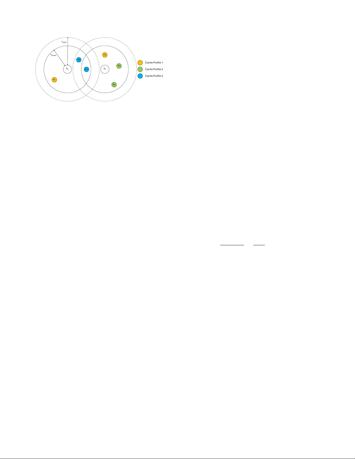
1 F airness Scheduling for Coded Caching in Multi-AP W ireless Local Area Networks Kagan Akcay , MohammadJav ad Salehi, and Giuseppe Caire Abstract —Coded caching (CC) schemes exploit the cumulativ e cache memory in the user’s devices and linear coding to turn uni- cast trafﬁc (individual ﬁle requests) into a multicast transmission. For a variety of carefully crafted network topologies, information theoretic optimality results sho wing large gains with respect to con ventional uncoded caching have been pro ved. However , the beneﬁts and suitability of CC for practical scenarios, such as con- tent streaming over existing wireless networks, hav e not yet been fully demonstrated. In this work, we study CC for on-demand video streaming over large Wir eless Local Area Networks, where multiple users are served simultaneously by multiple spatially distributed access points (APs). Users sequentially request video “chunks” of their selected video ﬁle in a given content library . T o enhance practical applicability , we pr opose a CC solution with a completely asynchronous, decentralized, and location- independent cache placement, paired with an “over IP” delivery mechanism operating in higher network layers and leaving the underlying physical and MA C layers untouched. For this CC scheme, we formulate the region of achievable goodput , deﬁned as the number of video chunks per unit time deliver ed in the users’ playback buffer , and formulate the goodput fairness problem in terms of a conv ex maximization problem. W e then propose an associated dynamic scheduling algorithm that provably achieves the optimal fairness point in stationary conditions with reduced complexity , and then introduce a heuristic to further reduce the complexity , ultimately achie ving a favorable trade-off between performance and complexity . W e illustrate the performance of the proposed solutions by comparing them with standard baseline schemes such as 1) con ventional (preﬁx) caching; 2) collision av oidance by allocating APs on orthogonal sub-channels with a certain spatial reuse; and 3) a CSMA-inspired solution where the APs trigger their activity via exponentially distributed waiting times and obey the ready-to-send/clear -to-send distributed coor- dination function. Our results show that CC can be implemented as an over IP solution in a scalable, compatible way with existing WLAN standards, achieving signiﬁcant gains ov er all the considered baseline approaches. Index T erms —coded caching, multi-AP WLANs, video stream- ing, fairness scheduling. I . I N T R O D U C T I O N A. Motivation and Prior Art The increasing amount of data trafﬁc, especially dri ven by multimedia applications, necessitates the development of new communication techniques [2]. One interesting resource is on- device memory; it is cheap and can be used to proactively store a large part of multimedia content, e.g., for video-on- demand and extended reality applications [3]. As a result, K. Akcay and G. Caire are with the Electrical Engineering and Computer Science Department, T echnische Univ ersit ¨ at Berlin, 10587 Berlin, Germany . E-mails: kagan.akcay@tu-berlin.de and caire@tu-berlin.de. MJ Salehi is with the Centre for W ireless Communications, Univ ersity of Oulu, 90570 Oulu, Finland. E-mail: mohammadjavad.salehi@oulu.ﬁ. Part of this work has been presented at the IEEE GLOBECOM 2023, in Kuala Lumpur, Malaysia [1]. many researchers have considered the efﬁcient use of onboard memory in the context of caching . Pioneering works in this regard introduced femtocaching [4] and F-RAN models [5]. A major theoretical breakthrough is the introduction of coded caching (CC) [6], which shows a gain factor in the content deliv ery rate proportional to the cumulative cache size in the network by lev eraging the differences in user cache memories to turn unicast data trafﬁc (i.e., satisfying individual user ﬁle demands) into multicast transmissions. Since its introduction, CC has generated a v ast and inﬂuen- tial body of work at the intersection of information theory , network coding, and algebraic/combinatorial coding theory . For example, numerous works hav e built on the original CC framew ork of [6], e.g., for wireless [7], [8], multi-server [9], multi-antenna [10], [11], device-to-de vice (D2D) [12], shared- cache [13], [14], multi-access [15], dynamic [16], [17], and combinatorial [18] networks. While these works are mathematically elegant and often yield information-theoretic optimality results [19]–[21], their application to practical wireless systems remains challenging. In particular , most theoretical works on coded caching applied to wireless systems in volv e modiﬁcations to the physical layer that are incompatible with current wireless standards, such as the ability to perform CC precoding directly in the complex signal domain (e.g., multi-user MIMO precoding) [22]–[24]. Such modiﬁcations are incompatible with the structure of contemporary wireless systems, where CC is implemented at the “application layer” (i.e., abo ve the IP layer), while the PHY and MAC layers are standardized independently (e.g., IEEE 802.11 [25] and 3GPP [26]), and must support a wide variety of services beyond content delivery . As a result, there exists a fundamental gap between the theoretical de velopment of CC in wireless networks and the practice of on-demand video streaming, which today operates almost entirely abov e the IP layer and relies only on limited adaptations of scheduling and queue management mechanisms. Recognizing this practical constraint, [27] considered CC “ov er IP”, i.e., abo ve an existing network layer capable of multicast routing, by considering a network model based on carrier-sense multiple access (CSMA), reminiscent of a W iFi W ireless Local Area Network (WLAN) with multiple access points (APs). In [27], a server transmits data to multiple spatially distribut ed users through multiple APs where the signal transmitted by each AP is recei ved by all the users within a certain radius. A collision-type interference model consistent with CSMA is used, such that a packet is lost if a user recei ves the superposition of concurrent packets from different APs above a certain interference threshold (a 2 similar model is elaborated in this paper , see Section II). Using the multiround delivery method of [28] (which was later prov ed by [13] to be optimal for the shared-cache model), [27] considered a graph coloring approach to construct a spatial reuse pattern for the APs, with optimized AP-user assignment to minimize delivery time. Then, a heuristic scheme dubbed “ A valanche” was introduced to leverage the fact that, as APs ﬁnish serving their assigned users, they stop transmitting and they may free other users from interference. As a consequence, AP activ ation propagates through the network in a sort of av alanche ef fect, constrained by the standard W iFi distributed clear-to-send/ready-to-send coordination function [29]. While [27] established the relev ance of CC ov er IP for WLAN-type netw orks and demonstrated promising perfor- mance g ains, its solutions are inherently heuristic and do not optimize a well-deﬁned network-wide performance metric. Moreov er , [27] as well as the great majority of information- theoretic papers on CC (e.g., see [6], [7], [9]–[16], [18]–[21], [23], [24], as well as many others) focus on minimizing the worst-case (o ver the user demands) deli very time for the whole set of requested ﬁles. In this classical version of the CC prob- lem, it does not matter whether a user receiv es its requested ﬁle at the be ginning or at the end of the deli very time, as long as the deliv ery time over the whole network , under the worst-case demand conﬁguration, is minimized. While this formulation may be suited to ﬁle download applications, it is certainly not suited to media str eaming . In streaming (e.g., video), a very long content ﬁle (a video with a duration of sev eral minutes) is divided into equal-sized “chunks”, which are fetched sequentially via HTTP requests from the video client running on the user de vice [30]. The chunks contain relativ ely short segments of the video and must be deliv ered sequentially at a rate (slightly) higher than the playback rate at which the client buf fer is emptied by the video player application [31], [32]. Hence, the most relev ant performance metric is the delivery rate, expressed as the long-term time- av eraged number of chunks delivered per unit time. Furthermore, since multiple users share the same wireless resources and may not simultaneously experience high rates, it is essential to ensure fairness across users and to provide fair rates, a principle that underlies virtually all modern wireless scheduling algorithms [33]–[36]. B. Our Contributions Motiv ated by the above observ ations, this paper addresses the problem of CC-based video streaming over multi-AP W iFi- type networks from a fundamentally different perspecti ve than existing works. W e focus on the fairness scheduling pr oblem in a multi-AP network obeying a collision-type W iF i-like interference model. 1 In CC, some se gments of the chunks, referred to as subpack ets , are placed in the user cache memory during the cache placement phase. Howe ver , a chunk is useless to the video player until all the subpackets forming the chunk are delivered. In the follo wing, we refer to the (time-averaged) rate at which chunks are made av ailable to the user as the goodput of the user . 1 The interference collision model is a convenient idealization of the actual W iFi MA C layer , and it is chosen here for the sake of analytical tractability . W e obtain the achiev able users’ goodput region as the con- ve x hull of all instantaneous delivery rate vectors. The fairness scheduling problem is then formulated as the maximization of a concave, component-wise non-decreasing network utility function [37] over the goodput region. T o enable continuous streaming, user goodputs must exceed the video playback rate [31], [32]. The utility function that directly enforces this requirement is hard fairness, which maximizes the minimum user goodput. Howe ver , when proportional fairness is em- ployed, at the expense of a reduction in the goodputs of some users, most users can stream at signiﬁcantly higher quality when adaptiv e quality coding is used [38]. Accordingly , in this paper we consider both hard fairness and proportional fairness as network utility functions. Although the formulated fairness scheduling problem is con ve x, its direct solution is not applicable to dynamic net- works, and the number of variables (i.e., the number of maxi- mal instantaneous rate vectors) gro ws faster than exponentially with the network size. T o enable applicability to dynamic networks, we adopt the L yapunov Drift-Plus-Penalty (DPP) method [34]–[36] and e xploit symmetry among users with identical cache proﬁles to signiﬁcantly reduce computational complexity . For larger networks, where exact optimality be- comes intractable, we introduce a principled heuristic that further reduces complexity by prioritizing transmissions to users with large queue backlogs within the DPP framework, achieving a fa vorable trade-of f between performance and com- plexity . W e demonstrate the ef fectiveness of the proposed frame- work through extensiv e simulations. As baseline schemes for comparison, we consider: 1) con ventional (i.e., preﬁx) caching; 2) a spatial reuse–based scheme, where APs are allocated orthogonal transmission resources (e.g., orthogonal W iFi channels [39], [40]) to avoid mutual interference, and where each AP maximizes its weighted sum rate according to the DPP method [34]–[36]; and 3) a CSMA-inspired solution in which APs are activ ated according to i.i.d. exponentially distributed waiting times and transmit only if the y do not create interference with users already being served by other activ e APs, following the standard distributed coordination function. Our results show that: 1) for all schemes, CC yields a sig- niﬁcant gain compared to con ventional (e.g., preﬁx) caching, due to its ability to exploit multicast transmissions; and 2) the proposed optimal scheme (when computationally feasible –e.g., with less than ten APs in the network) and the proposed principled heuristic (for very large netw orks) signiﬁcantly outperform all baseline schemes. T o the best of our knowledge, this work provides the ﬁrst rigorous scheduling framew ork for CC-based streaming over multi-AP WiFi-type networks that explicitly targets fair user goodput, thereby bridging the gap between the theoretical promise of coded caching and its practical deployment in real- world WLAN scenarios such as crowded venues, transporta- tion hubs, and in-ﬂight entertainment systems. Notation: V ectors are represented by bold letters, and sets are represented by calligraphic letters. v [ i ] is the i th element of vector v , and A\B denotes the set of elements of A not in B . For integer J , [ J ] represents the set { 1 , 2 , · · · , J } .  n k  3 4j                             C a c h e P ro f i le 1 C a c h e P ro f i le 2 C a c h e P ro f i le 3 Fig. 1: Example network with H = 2 , K = 6 , and L = 3 . denotes binomial coefﬁcient, and its value is zero if n < k . W e use the symbol  S k  , where S is a set, to denote the collection of all  |S | k  distinct subsets (combinations) of size k of the set S . I I . S Y S T E M M O D E L The network model considered in this work comprises a streaming server sending on-demand video streams to K wireless users via H APs. The server is connected to the APs through an error-free fronthaul network. W e use h i and u k , i ∈ [ H ] and k ∈ [ K ] , to denote APs and users, respecti vely . Fig. 1 illustrates a simple network with H = 2 and K = 6 . APs have an effecti ve transmission radius of r trans and an interference radius of r inter ≥ r trans . W e call an AP h i active at a gi ven time slot if it is transmitting data in that slot. According to the collision model, denoting the locations of the AP h i as x ( h i ) and user u k as x ( u k ) where x ( h i ) , x ( u k ) ∈ R 2 , u k can successfully receive the message (packet) sent by h i if and only if the following two conditions are satisﬁed: 1) | x ( h i ) − x ( u k ) | ≤ r trans ; and 2) there is no other acti ve AP node h i ′ such that | x ( h i ′ ) − x ( u k ) | ≤ r inter . In video streaming, each video ﬁle is split into a sequence of “chunks” corresponding to a fe w seconds of the video. For example, consider movies of duration ∼ 90min, and video chunks of duration ∼ 10sec, resulting in a sequence of 540 chunks, whereas at a typical video-coding rate of 2Mb/s, each chunk is 20Mb in size. The solutions proposed in this paper apply at the chunk level. W e assume that the video library consists of N ﬁles, each split into E chunks. Each user can cache γ N E chunks in its memory , for some γ ∈ [0 , 1] . A streaming user generates a sequence of requests for the corresponding chunks of its desired video ﬁle. Users pre-store a portion γ of each video chunk, so after each request, only the portion (1 − γ ) of the chunk that is not already in the user’ s cache must be deli vered. On-demand streaming sessions are generally asynchronous. This is because synchronous requests from a subset of users require not only that the users stream the same movie, but also that they start streaming within the same time frame of a few seconds (corresponding to the length of each video chunk). This implies that conv entional broadcasting, as in li ve TV where all users “see the same thing at the same time, ” is not possible in this setting. I I I . C O D E D C AC H I N G I N M U LT I - A P N E T W O R K S Follo wing the standard CC setting [6], system operation consists of two phases: placement and delivery . The placement phase is done ofﬂine, while deliv ery takes place during the streaming session. 2 A. Placement Phase During the placement phase, users’ cache memories are ﬁlled up with subpackets (i.e., smaller portions) of each video chunk, such that a fraction γ of each video chunk of each ﬁle is cached. In order to allow users to join and leav e the network and to start their streaming sessions at any time, it is of fundamental importance that the cache placement be completely decentralized. For this purpose, we follow the scheme of [27], [28] that consists of generating L distinct cache pr oﬁles and let each user randomly pick one proﬁle during its ofﬂine caching phase. The number of cache proﬁles L is an important system design parameter . Since the subpacketization is repeated identically for each chunk of each video ﬁle, we shall simply denote a generic chunk by W of size | W | bits. Assuming that t = γ L is an integer , 3 ev ery chunk W is partitioned into  L t  equal-sized subpackets W S , index ed by all possible subsets S ∈  [ L ] t  . For all l ∈ [ L ] , the l -th cache proﬁle Φ l is the collection of all subpackets W S such that S ∋ l , for all chunks of all ﬁles in the library . Since each subpacket has size | W | /  L t  bits and exactly  L − 1 t − 1  subpackets per chunk are included in Φ l , it is immediate to check that the number of cached bits per chunk of each ﬁle in the library is giv en by | W |  L − 1 t − 1   L t  = | W | t L = | W | γ , such that the size of each cache proﬁle Φ l is equal to a fraction γ of the whole library , as required. W e denote by L ( u k ) ∈ [ L ] the cache proﬁle assignment of u k , i.e., if L ( u k ) = l then user u k stores the cache proﬁle Φ l . Example 1. Consider the network in F ig. 1, which consists of H = 2 APs and K = 6 users, with L = 3 cache pr oﬁles. Each user is assigned to a cache pr oﬁle as indicated in the ﬁgur e. Suppose that each user can cache γ = 1 / 3 of the library , i.e., t = γ L = 1 . The cache pr oﬁles are obtained by dividing each chunk of every ﬁle into  3 1  = 3 subpack ets. Letting W denote a generic chunk and W { 1 } , W { 2 } , W { 3 } denote the corr esponding thr ee subpackets, cache proﬁle Φ 1 contains all subpack ets of type W { 1 } (i.e., all ﬁrst subpack ets of eac h chunk of each ﬁle), cache pr oﬁle Φ 2 contains all subpackets of type W { 2 } , and cache pr oﬁle Φ 3 contains all subpackets of type W { 3 } . Notice that multiple users may be assigned to the same cache pr oﬁle, since the assignments ar e made at random and independently for each user . F or example, here we have that users u 1 , u 4 ar e assigned to Φ 1 , u 5 , u 6 to Φ 2 , and u 2 , u 3 to Φ 3 . 2 For e xample, think of a “bring-your -own device” service where users cache segments from a library at home and then stream a particular movie from the library when the y join the network (e.g., in a train station, or airport terminal). 3 If γ L is not an integer , the scheme can be modiﬁed by cache sharing between two schemes with t 1 = ⌊ γ L ⌋ and t 2 = ⌈ γ L ⌉ . This is well-known in the CC literature and will not be further discussed here. 4 Remark 1. It is important to observe that the conv entional “preﬁx” caching [41], where each user caches the initial γ - fraction of each chunk, corresponds to a special case of the abov e scheme with L = 1 , i.e., where all users have the same cache proﬁle. Therefore, our framework for L = 1 en- compasses immediately the case of a con ventional (uncoded) caching system. ♢ B. Delivery Phase During the delivery phase, users request the chunks of their desired video ﬁle sequentially . As mentioned earlier, users can start streaming at any time, and once they begin streaming, they repeatedly generate requests for consecuti ve video chunks. In other words, after receiving a chunk, each user immediately generates a new request for the subsequent chunk. W e assume that a centralized scheduler (run at the server) makes sequential scheduling decisions at each gi ven time slot, coinciding with a video chunk duration. Notice that the scheduler time slots are generally much longer than the underlying PHY and MAC data packets since the scheduler operates “abov e IP”. For example, for a PHY channel rate of 20Mb/s and chunks of 20Mb, the scheduler makes a decision (roughly) every 1 sec. At each slot, gi ven the set of user requests, the scheduler creates code wor ds and sends them through the fronthaul to the APs, such that a subset of users can receive the codew ords via a subset of activ e APs. The determination of which users should receiv e and which APs should transmit, and the corresponding codeword formation at each time slot, deﬁnes a scheduling decision . Consequently , a sequence of scheduling decisions forms a scheduling policy [34]. At each giv en slot, we deﬁne the instantaneous delivery rate of each user as the amount of video-coded bits made av ailable to the user’ s playback buf fer in the gi ven slot, normalized by the length | W | of one chunk. The instantaneous deliv ery rate at each giv en slot depends on the scheduling decision for that slot. W e also deﬁne the user’ s goodput as the long-time av erage of the instantaneous deli very rate ov er a long sequence of slots. The user’ s goodput depends on the scheduling policy . W e shall ﬁrst clarify these concepts using our running example, and then in full generality . Example 2. Consider the network in Example 1 and denote the chunks requested by a user u k , k ∈ [6] , as W d k . Consider a scheduling decision wher e AP h 1 is idle (no tr ansmission in the curr ent time slot) and users u 3 , u 4 , u 5 ar e served by AP h 2 . W ith the cache placement in Example 1, the list of cached and r equested subpack ets by users u 3 − u 5 is as follows: Hence, User Cached Requested u 3 W d k , { 3 } , ∀ k ∈ [6] W d 3 , { 1 } , W d 3 , { 2 } u 4 W d k , { 1 } , ∀ k ∈ [6] W d 4 , { 2 } , W d 4 , { 3 } u 5 W d k , { 2 } , ∀ k ∈ [6] W d 5 , { 1 } , W d 5 , { 3 } AP h 2 can transmit (in multicast) the codewor ds X ( u 3 , u 4 ) = W d 3 , { 1 } ⊕ W d 4 , { 3 } , X ( u 3 , u 5 ) = W d 3 , { 2 } ⊕ W d 5 , { 3 } , X ( u 4 , u 5 ) = W d 4 , { 2 } ⊕ W d 5 , { 1 } , wher e ⊕ denotes the bit-wise XOR operation over the whole subpack et. It is readily seen that users u 3 , u 4 , and u 5 can r etrieve their desired subpack ets. F or example , user u 3 has W d 4 , { 3 } and W d 5 , { 3 } in its cache and therefor e can r etrieve W d 3 , { 1 } and W d 3 , { 2 } by simple XOR-ing the ﬁrst two code- wor ds, and so can also do users u 4 and u 5 . The length of each codewor d is equal to the length of a subpacket, such that sending the thr ee code wor ds r equir es one c hunk unit time. At the end of this transmission, users u 3 , u 4 , and u 5 have r etrieved all the missing subpack ets of their requested chunk, i.e., | W | usable bits in their playback buffer , while users u 1 and u 2 have not r eceived anything. Therefor e, the instantaneous rate vector corr esponding to this scheduling decision is (0 , 0 , 1 , 1 , 1) . C. Codewor d F ormation In general, a network with H APs has 2 H − 1 AP activation patterns where at least one AP is acti ve. W e denote activ ation patterns by binary vectors p j ∈ { 0 , 1 } H , j ∈ [2 H − 1] . The activ ation pattern determines which users can be served by each acti ve AP . This information, combined with users’ cache proﬁles, yields the CC code word formation. In CC, a code word can be created for every multicast subset of users T of size 0 < |T | ≤ t + 1 , where T must be formed by users with distinct cache proﬁles. Due to multiple choices for T for each activ e AP in a given activ ation pattern, there may e xist multiple candidate codew ords for each active AP . T o describe the codew ord formation in full generality , we need to introduce some notation. For a giv en activ ation pattern p j , consider an AP h i activ e in p j , i.e., such that p j [ i ] = 1 . Denote the set of users that can be served by h i as U i , i.e., U i includes users within distance r trans of h i but out of distance r inter of e very other active AP in p j . Also, for each l ∈ L , denote by U l i the subset of users in U i assigned to cache proﬁle Φ l , i.e., the users u k ∈ U l i with L ( u k ) = l . Some of these sets may be empty , and we let l ( i ) denote the number of such empty sets. T o create codew ords, we ﬁrst build a non-empty feasible subset V i of U i , where all users in V i hav e distinct cache proﬁles. Clearly , |V i | ≤ L − l ( i ) , and the number of possible ways to b uild V i is  Y l ∈ [ L ]  |U l i | + 1   − 1 , (1) where addition with one (inside parentheses) is to account for the case no user is selected from U l i , and the subtraction of one is to exclude the empty set. The users in V i can be served by a number of codewords transmitted by AP h i . These codewords are determined as follows: W e b uild the support set of V i as L ( V i ) = { L ( u k ) , ∀ u k ∈ V i } , (2) and then create its extended set ˆ V i by adding L − |V i | phantom users u ∗ l , 4 where L ( u ∗ l ) = l , for e very l ∈ [ L ] \L ( V i ) . Next, a pr eliminary codeword ˆ X ( ˆ T i ) can be built for every multicast 4 Phantom users are virtual users added only to maintain symmetry in the codew ord formation. The same concept is used in [24]. 5 subset ˆ T i of ˆ V i with maximal size | ˆ T i | = t + 1 as the XOR of subpackets ˆ X ( ˆ T i ) = M u k ∈ ˆ T i W d k , L ( ˆ T i ) \{ L ( u k ) } , (3) where L ( ˆ T i ) = n L ( u k ) , ∀ u k ∈ ˆ T i o , (4) and d k is the index of the video chunk requested by u k . Finally , the codew ord X ( T i ) is built from ˆ X ( ˆ T i ) by removing the presence of phantom users ( T i is the multicast set resulting by removing phantom users from ˆ T i ). Example 3. Consider again the network in Example 1 in F ig. 1. In Example 2, we pro vided transmitted codewor ds for this network when only h 2 is active. Now , let us consider a differ ent activation pattern p j = [1 , 0] , wher e only h 1 is active . F or the active AP h 1 , we have U 1 1 = { u 1 } , U 2 1 = ∅ , U 3 1 = { u 2 , u 3 } . Accor dingly , we have ﬁve options to choose the feasible set V 1 , given by { u 1 } , { u 2 } , { u 3 } , { u 1 , u 2 } and { u 1 , u 3 } . F or the choice V 1 = { u 1 , u 2 } , since L ( u 1 ) = 1 and L ( u 2 ) = 3 , we have L ( V 1 ) = { 1 , 3 } . The extended set is obtained by intr oducing the phantom user u ∗ 2 assigned to Φ 2 , i.e., ˆ V 1 = { u 1 , u 2 , u ∗ 2 } . As a r esult, we have three subsets ˆ T 1 of ˆ V 1 with size t + 1 = 2 , r esulting in the pr eliminary codewor ds ˆ X ( { u 1 , u 2 } ) = W d 1 , { 3 } ⊕ W d 2 , { 1 } , ˆ X ( { u 1 , u ∗ 2 } ) = W d 1 , { 2 } ⊕ W d 2 ∗ , { 1 } , ˆ X ( { u 2 , u ∗ 2 } ) = W d 2 , { 2 } ⊕ W d 2 ∗ , { 3 } . After remo ving the effect of the phantom user u ∗ 2 , the ﬁnal codewor ds are given as X ( { u 1 , u 2 } ) = W d 1 , { 3 } ⊕ W d 2 , { 1 } , X ( { u 1 } ) = W d 1 , { 2 } , X ( { u 2 } ) = W d 2 , { 2 } . D. Instantaneous Rate Calculation At each scheduling slot, the scheduler chooses an AP activ ation pattern p j and suitable codew ords as described abov e. W e let c ( p j ) denote the number of possible codewords for a giv en activ ation pattern p j . Formally , a scheduling decision ( j, s ) corresponds to the selection of activ ation pattern p j and code word choice s ∈ [ c ( p j )] . Let us consider an activ ation pattern p j and an activ e AP h i in p j . It can be easily veriﬁed that the codeword formation process described abov e guarantees that for a gi ven V i , each user u k ∈ V i obtains its requested chunk after n ( V i ) =  L t + 1  −  L − |V i | t + 1  (5) codew ord transmissions, where each transmission takes the length of one subpacket, i.e., | W | /  L t  bits. Hence, the instan- taneous deliv ery rate of each user u k ∈ V i is giv en by r ( V i ) = | W | n ( V i ) | W | ( L t ) =  L t  n ( V i ) . (6) Note that r ( V i ) in (6) is calculated according to the fact that  L −|V i | t +1  preliminary codewords ˆ X ( ˆ T i ) are ignored, i.e., not transmitted, as they include only phantom users. Now , to ﬁnd the instantaneous rate vector r ( j, s ) containing the instantaneous rates of all users in the network, we need to: 1) for each activ e AP { h i : p j [ i ] = 1 } , choose the feasible set V i ; 2) for each u k ∈ V i , set the element k of the vector r ( j, s ) equal to r ( V i ) as in (6); 3) ﬁll other elements of r ( j, s ) with zeros. Remark 2. Notice that for ﬁxed L and t , r ( V i ) depends only on |V i | ; it decreases as |V i | is increased up to |V i | = L − t , but then remains ﬁxed when L − t ≤ |V i | ≤ L . This is an important feature which will be exploited when we dev elop the reduced-complexity dynamic solution in Section V -A. ♢ Example 4. Consider the same network in Example 1, and assume the activation pattern is p j = [1 , 0] . F or active AP h 1 with V 1 = { u 1 , u 2 } , we get the thr ee codewor ds shown in Example 3. The tr ansmission of these three codewor ds r equir es one slot and delivers one chunk to users u 1 and u 2 and nothing to the other users, yielding the instantaneous rate vector (1 , 1 , 0 , 0 , 0) . Similarly , it can be seen that for V 1 = { u 1 } , we get two codewor ds X ( { u 1 } ) = W d 1 , { 2 } , X ( { u 1 } ) = W d 1 , { 3 } . The transmission of these two codewor ds r equir es 2 / 3 of a slot and delivers one chunk to user u 1 , yielding the instantaneous rate vector ( 3 2 , 0 , 0 , 0 , 0) . I V . F A I R N E S S S C H E D U L I N G As discussed in Section III, each scheduling decision ( j, s ) results in an instantaneous rate vector r ( j, s ) , where the k - th element, k ∈ [ K ] , is the number of useful bits made av ailable to user u k in the scheduling slot under decision ( j, s ) , normalized by the chunk size. A scheduling policy consists of a sequence of scheduling decisions { ( j t , s t ) : t = 1 , 2 , . . . } , whereas the goodput K -tuple (a vector in R K + ) achieved by a giv en scheduling policy is given by the long-term time average ¯ r = lim T →∞ 1 T T X t =1 r ( j t , s t ) , (7) if such a limit exists. It is well-known [34] that the goodput region of the netw ork is gi ven by the con vex hull of all instantaneous rate vectors, i.e., R = Con v  r ( j, s ) : j ∈ [2 H ] , s ∈ [ c ( p j )]  . (8) Since the number of instantaneous rate vectors is ﬁnite, R is a conv ex polytope in R K + . Furthermore, any point in the goodput region can be achiev ed by some randomized stationary scheduling policy , i.e., a policy that at each slot chooses (independently o ver the time slots) decision ( j , s ) with probability π ( j, s ) [34]. In general, we are interested in scheduling policies that operate the system on the Pareto boundary of R . Ho wev er , the choice of the operating point may correspond to different criteria of optimality . Follo wing [34], the operating point of the scheduler is determined as the point of the goodput region that maximizes a suitable network utility function of the user goodputs. By choosing a concav e componentwise non- decreasing network utility function, one can impose a desired fairness criterion. For example, we may choose any function from the well-known and widely used α -fairness family [37]. In particular , for α = 1 the corresponding fairness criterion is 6 referred to as pr oportional fairness , for α = 0 , the scheduler maximizes the sum over the goodputs (generally unfair), and for α → ∞ , we obtain max-min (or “hard”) fairness. W e focus on proportional fairness and hard fairness, corresponding to the maximization of the network utility functions f pf ( ¯ r ) : = X k log( ¯ r [ k ]) (9) for proportional fairness (PF), and f hf ( ¯ r ) : = min k ¯ r [ k ] (10) for hard fairness (HF). Remark 3. Maximizing the PF function is, in fact, equiv alent to maximizing the geometric mean of the users’ goodput vector . This is because we have 1 K X k log( ¯ r [ k ]) = log Y k ( ¯ r [ k ]) ! 1 K . (11) In this regard, we shall present PF results in terms of the goodput geometric mean to compare the proposed schemes in Section VI. ♢ A. The Optimization Pr oblem The maximization of the network utility function and the determination of the corresponding optimum goodput point in R , can be concisely stated as arg max f ( ¯ r ) , f ∈ { f pf , f hf } , s.t. ¯ r ∈ R . (12) Since the objectiv e functions are concave, (12) is a conv ex problem. Howe ver , it is generally difﬁcult to describe the con ve x polytope R in terms of linear inequalities (i.e., its supporting hyperplanes). Since each point of R is achiev able by a stationary policy , Problem (12) can be restated in an equiv alent form in terms of the probabilities { π ( j, s ) } that deﬁne a stationary policy . This yields arg max f ( ¯ r ) , f ∈ { f pf , f hf } , s.t. ¯ r = X j ∈ [2 H − 1] X s ∈ [ c ( p j )] π ( j, s ) r ( j, s ) , π ( j, s ) ≥ 0 , X j ∈ [2 H − 1] X s ∈ [ c ( p j )] π ( j, s ) = 1 . (13) Notice that this problem requires the enumeration of all (max- imal) instantaneous rate vectors. A maximal vector in a set of vectors in R K is a vector that is not componentwise dominated by any other vector in the set. It is clear that the sum over ( j, s ) in (13) can be restricted to maximal instantaneous rate vectors without loss of optimality . Howe ver , this is generally a very hard task unless the network is very small. In fact, there exist 2 H − 1 activ ation patterns, and the number of scheduling decisions per active AP giv en an acti vation pattern is giv en by (1). This means that, the number of scheduling decisions ( j, s ) , i.e., v ariables π ( j, s ) in (13) is approximately giv en by X j ∈ [2 H − 1] Y i ∈ [ H ] , p j [ i ]=1 Y l ∈ [ L ] ( |U l i | + 1) . (14) For ﬁxed L , this number gro ws faster than exponentially when H and the number of users inside the AP transmission radii increase, i.e., when |U l i | increases for each i and l . As a quick example, for a network of only H = 4 APs and L = 4 , ev en for just 2 user from each cache proﬁle and a total of 8 users that can be served by each AP simultaneously , the single activ ation pattern p j = (1 , 1 , 1 , 1) yields a number of scheduling decisions equal to 3 16 ≈ O (10 7 ) . Remark 4. In fact, the complexity order in (14) is an upper bound to the real complexity value. This is because, it can be inferred from Remark 2 that for a giv en activ ation pattern p j and activ e AP h i , some feasible sets do not need to be considered when forming the codeword, i.e., if L − l ( i ) > L − t , one does not need to consider the feasible sets V i with L − t ≤ |V i | < L − l ( i ) , as the users’ individual rates won’t change in this re gion and the corresponding rate v ector will be dominated by the rate vector using all the L − l ( i ) users in codew ord formation. Nev ertheless, ev en after applying this reduction, the general scaling law of the complexity order will remain unchanged, and solving the optimization problem will still be infeasible for large networks. Furthermore, certain activ ation patterns in which only a small subset of APs is active need not be considered if activ ating additional APs does not introduce any interference among all the users that can be chosen for the codew ord formation. For instance, if the interference radii of h 1 and h 2 do not overlap and are sufﬁciently separated, it is redundant to compute instantaneous rate vectors corresponding to cases in which only one of the two APs is active, since any such rate vector is dominated by a rate vector obtained when both APs are activ ated. Howe ver , the set of activ ation patterns that can be discarded, if any , depends on the speciﬁc network topology . ♢ B. Complexity Reduction The complexity of the optimization problem (13) can be reduced by noticing that some users in the network are equiv- alent . T wo users are equivalent if they have the same cache proﬁle and the same spatial properties, i.e., if both of them are within the transmission and interference radii of the same APs. It is easy to see that if two users are equiv alent, then the instantaneous rate vectors are symmetric in such users in the following sense: suppose that u k and u ˜ k are equiv alent users and consider an instantaneous rate vector r with k -th element r [ k ] > 0 (clearly , r [ ˜ k ] = 0 as u k and u ˜ k hav e the same cache proﬁle and therefore cannot be served together in the same multicast group). Then, there exists another instantaneous rate vector ˜ r such that ˜ r [ ˜ k ] = r [ k ] , ˜ r [ k ] = 0 , and ˜ r [ k ′ ] = r [ k ′ ] for all k ′  = k , ˜ k . Furthermore, it can be easily veriﬁed that the solution of the optimal fairness point problem (13) assigns equal probability to the rate vectors r and ˜ r . By grouping users into equi valent classes with respect to the abov e deﬁned equiv alence relation (notice that some equiv alent classes are indeed singletons, since there may be users that are not equiv alent to any other user), the complexity of the network can be reduced by retaining only one representativ e user for each equi valent class. After computing the set of instantaneous rate vectors for the reduced network, the set of rate vectors for the original network can be obtained simply by expanding each class representativ e rate entries into a uniform (equal entries) subvector , of length equal to the size of the corresponding equiv alent class, and entries that sum up to 7 the rate of the representativ e. For example, if user u k is the representativ e of a class of (say) ℓ users and, for a gi ven scheduling decision ( j, s ) in the reduced network, receiv es an instantaneous rate of r k , the ℓ elements of the rate vector of the original network corresponding to the equiv alent class will all be equal to r k /ℓ . The equiv alent user approach yields some moderate com- plexity reduction with respect to the direct formulation of problem (13). Nevertheless, it remains unsuitable for scaling to large networks. Example 5. Consider the network in F ig. 1. F or this network, we have put the maximal instantaneous rate vectors and the r esults of the optimization pr oblem in (13) for both PF and HF in T able I. The ﬁrst column in T able I includes the case wher e equivalent users ar e not consider ed. As can be seen, ther e exists a total number of 11 maximal instantaneous rate vectors in this case. However , it can be easily veriﬁed from F ig 1 that u 5 and u 6 ar e equivalent users, as they are both assigned to cache pr oﬁle Φ 2 , are within the transmission radius of h 2 , and outside of the transmission radius of h 1 . This is also evident fr om the ﬁrst column of T able I, as u 5 and u 6 ar e symmetric in instantaneous rate vectors { r (2 , 1) , r (2 , 2) } , { r (3 , 1) , r (3 , 2) } , and { r (3 , 4) , r (3 , 5) } . As a result, one can r etain one of them as the class r epresentative user , and calculate the rate vectors for the r educed network, as shown in the second column of T able I. By e xpanding the rate vectors and solving the optimization pr oblem, as shown in the third column of T able I, ﬁnal rate and fairness function values r emain unchanged, while the number of maximal rate vectors is reduced from 11 to 8 . As an extra note, we notice also from T able I that since u 5 and u 6 shar e the network r esour ces equally , π pf (2 , 1) = π pf (2 , 2) = 1 2 ˜ π pf (2 , 1) and π pf (3 , 1) = π pf (3 , 2) = 1 2 ˜ π pf (3 , 1) , and a similar pattern also holds for HF . V . D Y NA M I C S C H E D U L I N G S O L U T I O N S The solution to (13) yields a stationary scheduling policy that maximizes the desired network utility function. Howe ver , the resulting scheduler is “static”, in the sense that it will choose decision ( j, s ) with probability π ( j, s ) irrespectiv e of the actual status of chunk deliv ery to the users. Hence, opti- mality is approached only in the limit of a very long averaging time, and the actual sample paths of the deliv ery process for any giv en user (i.e., the number of delivered chunks per unit time averaged over a short window of slots) may actually deviate signiﬁcantly from the long-term av erage. In addition, such a policy must be recalculated as the network topology changes, for example, when ne w users start streaming and/or when currently streaming users stop. Using the well-known theory de veloped in [34]–[36], a dynamic policy based on the L yapunov DPP method can be readily obtained by deﬁning a vector of recursiv ely updated priority weights Q t ∈ R K + , usually referred to as virtual queue backlogs , with update equation Q t +1 = [ Q t − R t ] + + A t , (15) where [ · ] + indicates the (componentwise) positiv e part, R t is an instantaneous rate vector , and A t is the vector of virtual arrival pr ocesses at slot time t . The DPP scheduler iterates the following three steps: 1) V irtual arriv al determination as the solution of the auxil- iary optimization problem: A t = arg max a ∈ [0 ,A max ] K V f ( a ) − a T Q t , (16) where V > 0 and A max > 0 are two control parameters. 2) Instantaneous rate determination as the solution of the weighted sum-rate maximization (wsrm) problem R t = arg max r ∈{ r ( j,s ) } r T Q t . (17) 3) Update of the virtual queues according to (15). The scheduler is initialized with a suitable initial backlog value, e.g., Q 0 = 0 . It can be shown that for a stationary network (in our case, for ﬁxed topology and user streaming activity), the long term average ¯ r dpp of the instantaneous rates produced by the DPP algorithm satisﬁes the optimality condition f ( ¯ r dpp ) ≥ f ( ¯ r ⋆ ) − O (1 /V ) (18) where ¯ r ⋆ is the solution of (12) and O (1 /V ) is a term that decreases as 1 /V , provided that the hypercube [0 , A max ] K contains R . In our case, this condition is trivially satisﬁed by noticing from (6) that the instantaneous rate of any user cannot be larger than  L t  , therefore R is necessarily contained in the hypercube [0 , A max ] K for A max =  L t  . The auxiliary problem (16) is con vex and easily solved in closed form for the class of α -fairness functions f . In particular , for f ( · ) = f pf ( · ) the solution of (16) is given by A t [ k ] = min  V Q t [ k ] , A max  , (19) and for f ( · ) = f hf ( · ) , the solution is giv en by A t [ k ] = ( A max if V > P k Q t [ k ] , 0 otherwise . (20) In contrast, the instantaneous wsrm in (17) is a very hard com- binatorial problem since we need to search ov er all possible (discrete) maximal instantaneous rate vectors { r ( j, s ) } . A. Reduced-Complexity Dynamic Solution One main source of complexity in solving the wsrm (17) is that, for each AP acti vation pattern, a typically large number of scheduling decisions (i.e., options for CC codeword formation) exist. Here, we consider an approach that constructs a reduced set of candidate instantaneous rate vectors containing the optimal solution of the wsrm by taking into account the properties of users with the same cache proﬁle served by the same activ e AP and their queue weights in Q t . W e refer to this reduced complexity solution of (17) as “dynamic” since the construction of the reduced set of candidate instantaneous rate vectors is based on the queue weights Q t , which is dynamically updated via (15). Consider an acti vation pattern p j and a subset of users K ⊆ [ K ] , where all users in K are assigned the same cache proﬁle and can be served by the same active AP h i in p j . For this subset, the following properties hold: 8 Activation pattern Original rate vectors Reduced rate vectors ( u 5 and u 6 merge) New rate vectors (generated from reduced ones) p 1 = (1 , 0) r (1 , 1) = (1 , 1 , 0 , 0 , 0 , 0) , r (1 , 2) = (1 , 0 , 1 , 0 , 0 , 0) , r (1 , 3) = (0 , 1 . 5 , 0 , 0 , 0 , 0) r (1 , 4) = (0 , 0 , 1 . 5 , 0 , 0 , 0) ˜ r red (1 , 1) = (1 , 1 , 0 , 0 , 0) ˜ r red (1 , 2) = (1 , 0 , 1 , 0 , 0) ˜ r red (1 , 3) = (0 , 1 . 5 , 0 , 0 , 0) ˜ r red (1 , 4) = (0 , 0 , 1 . 5 , 0 , 0) ˜ r (1 , 1) = (1 , 1 , 0 , 0 , 0 , 0) ˜ r (1 , 2) = (1 , 0 , 1 , 0 , 0 , 0) ˜ r (1 , 3) = (0 , 1 . 5 , 0 , 0 , 0 , 0) ˜ r (1 , 4) = (0 , 0 , 1 . 5 , 0 , 0 , 0) p 2 = (0 , 1) r (2 , 1) = (0 , 0 , 1 , 1 , 1 , 0) r (2 , 2) = (0 , 0 , 1 , 1 , 0 , 1) ˜ r red (2 , 1) = (0 , 0 , 1 , 1 , 1) ˜ r (2 , 1) = (0 , 0 , 1 , 1 , 0 . 5 , 0 . 5) p 3 = (1 , 1) r (3 , 1) = (1 . 5 , 0 , 0 , 1 , 1 , 0) r (3 , 2) = (1 . 5 , 0 , 0 , 1 , 0 , 1) r (3 , 3) = (1 . 5 , 0 , 0 , 1 . 5 , 0 , 0) r (3 , 4) = (1 . 5 , 0 , 0 , 0 , 1 . 5 , 0) r (3 , 5) = (1 . 5 , 0 , 0 , 0 , 0 , 1 . 5) ˜ r red (3 , 1) = (1 . 5 , 0 , 0 , 1 , 1) ˜ r red (3 , 2) = (1 . 5 , 0 , 0 , 1 . 5 , 0) ˜ r red (3 , 3) = (1 . 5 , 0 , 0 , 0 , 1 . 5) ˜ r (3 , 1) = (1 . 5 , 0 , 0 , 1 , 0 . 5 , 0 . 5) ˜ r (3 , 2) = (1 . 5 , 0 , 0 , 1 . 5 , 0 , 0) ˜ r (3 , 3) = (1 . 5 , 0 , 0 , 0 , 75 , 0 . 75) Non-zero probabilities from (13) for PF π pf (1 , 3) ≈ 0 . 1667 π pf (2 , 1) = π pf (2 , 2) ≈ 0 . 2083 π pf (3 , 1) = π pf (3 , 2) ≈ 0 . 2083 − ˜ π pf (1 , 3) ≈ 0 . 1667 ˜ π pf (2 , 1) ≈ 0 . 4167 ˜ π pf (3 , 1) ≈ 0 . 4166 PF goodput vector ¯ r ⋆ pf ≈ (0 . 62 , 0 . 25 , 0 . 42 , 0 . 83 , 0 . 42 , 0 . 42) − ¯ r ⋆ pf ≈ (0 . 62 , 0 . 25 , 0 . 42 , 0 . 83 , 0 . 42 , 0 . 42) PF geometric mean 0 . 46 − 0 . 46 Non-zero probabilities from (13) for HF π hf (1 , 3) ≈ 0 . 2857 π hf (2 , 1) = π (2 , 2) ≈ 0 . 2143 π hf (3 , 4) = π (3 , 5) ≈ 0 . 1429 − ˜ π hf (1 , 3) ≈ 0 . 2857 ˜ π hf (2 , 1) ≈ 0 . 4286 ˜ π hf (3 , 3) ≈ 0 . 2857 HF goodput vector ¯ r ⋆ hf ≈ (0 . 43 , 0 . 43 , 0 . 43 , 0 . 43 , 0 . 43 , 0 . 43) − ¯ r ⋆ hf ≈ (0 . 43 , 0 . 43 , 0 . 43 , 0 . 43 , 0 . 43 , 0 . 43) HF minimum rate 0 . 43 − 0 . 43 T ABLE I: The maximal instantaneous rate vectors and the solution of (13) for the network in Fig 1, w/ and w/o considering the equiv alent users. • the users in K cannot recei ve simultaneous transmissions from h i , so only one user in the subset can attain a nonzero rate in any feasible instantaneous rate vector , and • since user rates are multiplied by their virtual queue backlogs in the objective function of (17), it is sufﬁcient to consider only the user with the largest queue backlog in K when forming the code word. Now , to reduce the number of instantaneous rate vectors for a giv en activ ation pattern p j , we proceed as follows: 1) F or each active AP h i and each cache proﬁle l where U l i is nonempty , ﬁnd the user with the largest queue backlog. Let C i denote the set of such users for all cache proﬁles. Clearly , |C i | = L − l ( i ) , since there are l ( i ) cache proﬁles where U l i is empty . 2) Consider only the users in {C i } i while forming the code- words, and ﬁnd the instantaneous rate vector maximizing the weighted sum-rate for the acti vation pattern p j by identifying and combining the multicast groups that yield the highest weighted sum-rate for each activ e AP . Notice that for a gi ven activ e AP h i , each of the L − l ( i ) users in C i has a different cache proﬁle, so one can create a multicast group, i.e., a feasible set, by using any combination of these users. Howe ver , from Remark 2 , we know that the instantaneous rate of the users in a feasible set V i depends only on |V i | ; it decreases as |V i | is increased up to |V i | = L − t , but then remains ﬁxed when L − t ≤ |V i | ≤ L . It follows that, for a gi ven acti ve AP h i , there are only z i = min( L − l ( i ) , L − t ) different rate values that the users in a feasible set can have. So, if L − l ( i ) > L − t , one does not need to consider the feasible sets V i with L − t ≤ |V i | < L − l ( i ) , as the users’ individual rates won’t change and the rate vector will be dominated by the rate vector using all the L − l ( i ) users in codew ord formation (similar discussion appeared also in Remark 4). As a result, for a giv en activ e AP h i , it is sufﬁcient to search for the largest weighted sum-rate among the z i different rate vectors, where only the users with the largest queue backlogs in C i are chosen in the codeword formation. This is accomplished by sorting the users in C i by their queue backlogs, from the largest to the smallest. Then, we create feasible sets V i,g , g ∈ [ z i ] , such that for g < z i , V i,g consists of the ﬁrst g users among the sorted ones, and for g = z i , V i,g consists of all the L − l ( i ) users in C i . By constructing the corresponding rate vector for each V i,g and solving the weighted sum-rate maximization over these z i rate vectors, we can ﬁnd the rate vector r ( i ) achieving the solution for an acti ve AP h i . Let w ( i ) denote the achie ved weighted sum-rate for r ( i ) . Then, the instantaneous rate vector for the activ ation pattern p j is giv en by r ( j, 1) = P p j [ i ]=1 r ( i ) and the corresponding weighted sum-rate by w j = P p j [ i ]=1 w ( i ) . This is con veniently illustrated by the follo wing example. Example 6. Let L = 5 , t = 2 , and w .l.o.g., for a given activation pattern p j and active AP h i , let l ( i ) = 1 , so there ar e 4 cache pr oﬁles wher e U l i is not empty . Assume also that C i = { u 1 , u 2 , u 3 , u 4 } , where Q 1 > Q 2 > Q 3 > Q 4 . Then, for h i , ther e are z i = 3 constructed rate vectors. The feasible sets, the corresponding rate vector s, and the r esulting weighted sum-rates ar e presented in T able II. Notice fr om T able II that since (1 , 1 , 1 , 0 , ..., 0) is dominated by (1 , 1 , 1 , 1 , 0 , ..., 0) , we can e xclude it fr om the solution of the weighted sum-r ate maximization. Steps 1 and 2 pro vide an instantaneous rate vector for each activ ation pattern and its corresponding weighted sum- rate. Then, to ﬁnd the solution to (17), we simply determine 9 Feasible set Rate vector W eighted sum-rate V i, 1 = { u 1 } ( 5 3 , 0 , ..., 0) 5 3 Q 1 V i, 2 = { u 1 , u 2 } ( 10 9 , 10 9 , 0 , ..., 0) 10 9 ( Q 1 + Q 2 ) V i, 3 = { u 1 , u 2 , u 3 , u 4 } (1 , 1 , 1 , 1 , 0 , ..., 0) Q 1 + Q 2 + Q 3 + Q 4 { u 1 , u 2 , u 3 } (1 , 1 , 1 , 0 , ..., 0) Q 1 + Q 2 + Q 3 T ABLE II: The feasible sets, the corresponding rate v ectors, and the resulting weighted sum-rates for the activ e AP h i in Example 6. the activ ation pattern j ∗ that maximizes the weighted sum- rate. So, the solution to (17) is gi ven by r ( j ∗ , 1) where j ∗ = arg max j ∈ [2 H − 1] w j . This solution reduces the number of scheduling decisions from (14) to 5 X j ∈ [2 H − 1] X i ∈ [ H ] , p j [ i ]=1 min( L − l ( i ) , L − t ) , (21) indicating a massive decrease in the number of considered scheduling decisions. For instance, notice that the term inside the summation over the activ ation patterns j ∈ [2 H − 1] is linear in H for ﬁxed L , instead of exponential as in (14). As an e xample, consider the same parameters as in the paragraph following equation (14): a network with H = 4 APs and L = 4 , where 2 users from each cache proﬁle and a total of 8 users can be served by each AP simultaneously . Assume also t = 1 . Then, for the activ ation pattern p j = (1 , 1 , 1 , 1) , by using the reduced-complexity dynamic solution, the number of scheduling decisions is reduced from O (10 7 ) to just 12 . B. The V irtual Queue Heuristic W e propose a heuristic for the DPP dynamic scheduler , suitable for very large netw orks where even the reduced- complexity solution in Section V -A is impractical. For these cases, we aim at obtaining a suboptimal but scalable to very large networks DPP dynamic scheduler by replacing the instantaneous weighted sum-rate maximization step in (17) with a heuristic choice of the AP acti vation pattern and corresponding CC code words. The idea is to fa vor serving users with large queue backlogs. The reasoning is that the weighted sum-rate in (17) increases when higher rates are assigned to such users. So, instead of solving (17) or the reduced-complexity dynamic solution by searching over all activ ation patterns, we ﬁnd a feasible activ ation pattern that prioritizes the users with large queue backlogs by assigning them to APs. The corresponding codewords and the rate vector are then determined accordingly . As a general description of the proposed heuristic, at each scheduling slot, we sort users by their virtual queue backlogs from largest to smallest. Then, the users are assigned to APs one by one. T o assign each user to an AP , we search for suitable APs: If there is a unique active AP that can serve a user and the user is not interfered with by another active AP , we check the weighted sum-rate in (17), and assign the user to the AP only if the resulting weighted sum-rate increases. If there is no acti ve AP that can serve the user , an inacti ve AP is randomly chosen among those that can serve the user (if any), provided that the user isn’t interfered with by any 5 Notice that for a given activation pattern p j and activ e AP h i , if z i = 1 , there is a unique resulting weighted sum-rate for h i . Hence, h i can be excluded from the computation in (21) for p j . Furthermore, if for a given p j all active APs h i satisfy z i = 1 , the number of scheduling decisions corresponding to p j reduces to one. currently activ e AP . In both cases, it is ensured that each activ e AP serves at most one user assigned to each cache proﬁle, and that interfering inactive APs remain inactiv e in the same scheduling slot. The steps of the proposed V irtual Queue Heuristic at each scheduling slot are giv en by the pseudocode in Algorithm 1 where we use the following notations: 1) t is the scheduling slot index; 2) H all denotes the set of all APs; 3) H denotes the set of candidate APs to be activ ated; 4) H on denotes the set of active APs; 5) w temp i denotes the temporary weighted sum-rate of the AP h i ; 6) m i , i ∈ [ H ] , is a vector of length L that expresses the “local cache population” of AP h i , i.e., for all i ∈ [ H ] , m i [ l ] = k only if AP h i is serving u k and L ( u k ) = l (otherwise, it is zero); and { m i } s denotes the set of users included in m i . W e have also used some auxiliary functions: 1) O R D E R ( u ) sorts the set of users { u k } according to Q t [ k ] v alues, in descending order; 2) I N T E R ( u k ) gives the set of activ e APs in H on which are within radius r inter of user u k ; 3) T R A N S ( u k ) giv es the set of APs in H which are within radius r trans of user u k ; and 4) W S R ( m i ) giv es the weighted sum-rate of AP h i , assuming the users in m i are assigned to h i . At the beginning of every scheduling slot t , we set H = H all , H on = ∅ , and m i to all-zero vector for ev ery i ∈ [ H ] . (Line 1 of Algorithm 1). The algorithm runs indeﬁnitely for each scheduling slot t , where users are assigned to APs and the resulting instantaneous rate vector r is calculated via iterations ov er the network. V I . N U M E R I C A L R E S U L T S First, we present simulations comparing the performance of the optimum solution, i.e., the solution to (13), or equi valently , the goodput vector achiev ed by (15)–(17), with that of: 1) the V irtual Queue Heuristic (Section V -B); 2) a con ventional uncoded caching scheme (see Remark 1), and 3) two addi- tional baseline schemes described below . Then, we simulate a dynamic network scenario to illustrate how users’ goodputs adapt to changes in the network. Streaming rates: W e assume that each AP has the same downlink multicast channel capacity , denoted by C . Recall that the goodput of a user is deﬁned as the time-averaged rate (normalized rate per unit time) at which video chunks are made av ailable to the user . Thus, for a given goodput ¯ r , the corresponding physical-layer rate at which a user receiv es video chunks is C ¯ r bit/s. In all the subsequent ﬁgures, each reported goodput value can be multiplied by the AP capacity C to obtain the actual (physical) streaming rate. Baseline schemes: In addition to con ventional (uncoded) caching, we use two other baseline schemes for comparison. The ﬁrst baseline, called reuse with queue update , uses standard channel reuse to av oid interference. A channel reuse scheme with reuse factor m av oids mutual interference be- tween neighboring APs by allocating them to m orthogonal channels so they do not collide. Each sub-channel is acti vated in round-robin (in time) or parallel on 1 /m of the av ailable bandwidth (in frequency). In our case, this corresponds to activ ating the non-neighboring APs in the same sub-channel ev ery m -th slot. 10 1: I N I T I A L I Z E 2: O R D E R ( u ) 3: for all u k ∈ u do 4: I k ← I N T E R ( u k ) 5: if |I k | == 1 then 6: h i ← I k [1] 7: if | x ( h i ) − x ( u k ) | ≤ r trans , m i [ L ( u k )] = 0 then 8: m i [ L ( u k )] ← k 9: if W S R ( m i ) < w temp i then 10: m i [ L ( u k )] ← 0 11: else 12: for all h i ′ ∈ H , h i ′  = h i do 13: if | x ( h i ′ ) − x ( u k ) | ≤ r inter then 14: Remov e h i ′ from H 15: if |I k | == 0 then 16: T k ← T R A N S ( u k ) 17: if |T k | > 0 then 18: h i ← T k [ r ng ] 19: m i [ L ( u k )] ← k 20: w temp i ← W S R ( m i ) 21: Add h i to H on 22: for all h i ′ ∈ H , h i ′  = h i do 23: if | x ( h i ′ ) − x ( u k ) | ≤ r inter then 24: Remov e h i ′ from H 25: for all h i ∈ H do 26: f or all l ∈ [ L ] , m i [ l ]  = 0 do 27: r [ m i [ l ]] ← r ( { m i } s ) 28: Compute the virtual arriv al vector using (16) 29: Update the virtual queue backlog using (15) 30: if t > 1 then 31: ¯ r [ k ] ← ( ¯ r [ k ] ∗ ( t − 1) + r [ k ]) /t 32: else 33: ¯ r [ k ] ← r [ k ] 34: t ← t + 1 Algorithm 1: V irtual Queue Heuristic The second baseline, called CSMA-inspir ed queue update , as its name suggests, is inspired by idealized CSMA mod- els [42], [43]. W ith this baseline, each AP is assigned a timer from an exponential distrib ution at the beginning of each scheduling slot. Depending on the timer v alues, APs are acti vated one by one, provided that the y don’ t create interference with users that are already being served by other activ e APs, obeying the ready-to-send/clear-to-send distrib uted coordination function. In both baseline schemes, interference is av oided. Therefore, the wsrm problem (17) restricted to the allowed AP activ ation patterns decouples into indepen- dent maximizations, one for each active AP . In other words, by using a standard collision-avoidance technique (reuse or CSMA), the baseline schemes reduce the weighted sum-rate maximization in (17) to a set of mutually disjoint smaller problems that can be solved with low complexity . Simulation setup: W e assume that H APs are located at the center of hexagons on a ﬁnite hexagonal grid. Each hexagon has a radius of 1 (normalized length unit), we set r trans = 1 and r inter = 1 . 2 . Notice that since the AP locations form a hexagonal grid, the minimum spatial reuse factor required to -3 -2 -1 0 1 2 3 -3 -2 -1 0 1 2 3 Fig. 2: Example network with H = 7 , K = 70 . Each green user is within the transmission radius of e xactly 1 AP and outside the interference radii of other APs. Each blue user is within multiple AP transmission/interference radii. Users Green Blue All Optimum Solution 0.27 0.22 0.14 V irtual Queue Heuristic 0.27 0.20 0.13 CSMA-Inspired Queue Update 0.27 0.17 0.10 Reuse with Queue Update 0.09 0.14 0.07 T ABLE III: Goodput geometric mean comparison of the users in Figure 2 for PF , with L = 5 , γ = 0 . 2 ; if only blue, only green, or all users are served. guarantee collision-free transmissions is m = 3 . In Figure 2 we plot a hexagonal grid that consists of H = 7 APs and K = 70 users. Each user is randomly placed within the transmission area of APs. The geometric means of the user goodputs for PF for the different user subsets are presented in T able III, where each user is randomly assigned to a cache proﬁle Φ l , l ∈ [ L = 5] . W e can see from T able III that when only green users are served, i.e., users located within the transmission radius of a single AP and outside the interference radii of all other APs, the geometric means of the optimum solution and CSMA- Inspired Queue Update are identical. This result is expected, since in this scenario e very AP can be activ ated at each scheduling slot, and regardless of which users an AP serves, those users won’t be interfered with by any other activ e AP . In both methods, each AP independently maximizes its weighted sum-rate, which is optimal. In the V irtual Queue Heuristic, all APs are also activ ated at each scheduling slot; ho wev er , because the weighted sum rates of all multicast groups are not exhaustiv ely e valuated (Recall from Section V -B that the weighted sum-rate is only checked when adding the next user), optimality is not guaranteed in general. Nev ertheless, we can see from T able III that for the considered network realization, the V irtual Queue Heuristic also attains the optimal performance when only green users are served. In contrast, Reuse with Queue Update assigns a priori distinct reuse numbers to neighboring APs, allo wing only APs with the same reuse number to be activ e simultaneously . In the absence of interference, such reuse constraints are unnecessary . Since each AP is activ ated only once ev ery three slots, the resulting geometric mean goodput is approximately one-third of the optimal value. When only blue users are served, i.e., users located within multiple AP transmission/interference radii, both the V irtual Queue Heuristic and the CSMA-Inspired Queue Update be- come suboptimal, as shown in T able III. The reason is that when multiple APs are activ ated simultaneously , interference occurs among some users. The V irtual Queue Heuristic sorts the user queue backlogs and assigns each user to an ap- 11 0 10 20 30 40 0 1 2 3 4 5 6 7 8 · 10 − 2 L Goodput Geometric Mean Optimum Solution V irtual Queue Heuristic CSMA-Inspired Queue Update Reuse with Queue Update Fig. 3: Goodput geometric mean for different values of L for PF , with H = 10 , K avg = 200 , γ = 0 . 1 . propriate AP sequentially . Even though the activ ation pattern depends on the queue backlogs since users with larger queue backlogs are prioritized, the choice of the acti vation pattern is still heuristic because the solution is not searched over all activ ation patterns, as in the optimum solution. This pre- vents some users from receiving any transmission in a giv en scheduling slot, even though they might recei ve transmission in the optimum solution. In CSMA-Inspired Queue Update, the activ ation order of the APs is random and independent of the queue backlogs, which further degrades performance and leads to worse results than the V irtual Queue Heuristic. The Reuse with Queue Update performs closer to the other methods in this case, since interference av oidance via reuse becomes more rele vant when serving blue users. Howe ver , it remains suboptimal because the ﬁxed reuse pattern is ov erly restricti ve. For instance, if a user within the transmis- sion/interference radii of only 2 APs is chosen to be served, one of the APs cannot be activ ated, but another 3 rd AP , neighboring both APs, can still be activ ated. Howe ver , this is not permitted in Reuse with Queue Update, resulting in worse than optimal performance. In fact, T able III shows that it performs the worst. Finally , when all users are served, T able III sho ws that the proposed schemes, i.e., the optimum solution and the V irtual Queue Heuristic, outperform the baseline schemes. W e also conduct Monte Carlo simulations in which users are distributed according to a homogeneous Poisson point process within the transmission area of the APs. The average number of users in the transmission area, denoted by K av g , is determined by the density of the Poisson point process. Each user is randomly assigned to a cache proﬁle Φ l , l ∈ [ L ] . W e set γ = 0 . 1 , H = 10 , and K av g = 200 , and compare the performance of different schemes in Figures 3-5. First, recall from Remark 1 that the case L = 1 in Figures 3 and 4 coincides with the conventional (i.e., uncoded) caching scheme (e.g., “preﬁx caching” [44]) and can be applied to each of the considered scheduling/transmission schemes by assuming that every user caches the same portions of each chunk. In this case, since no multicasting opportunities arise, the server transmits the requested portion of each chunk via standard unicast transmissions. In Figure 3, we plot the goodput geometric mean versus L ∈ { 1 , 10 , 20 , 35 , 40 } for PF for all the schemes. W e observe 0 5 · 10 − 2 0 . 1 0 . 15 0 . 2 0 . 25 0 0 . 2 0 . 4 0 . 6 0 . 8 1 Goodput Goodput CDF L = 1 L = 10 L = 20 L = 30 L = 40 Fig. 4: Goodput CDF for different values of L for HF for the optimum solution, with H = 10 , K avg = 200 , γ = 0 . 1 . that all the proposed schemes signiﬁcantly outperform the baseline schemes, as expected from the discussion following T able III. It can also be seen that the geometric means of the optimum solution, the V irtual Queue Heuristic, and the Reuse with Queue Update increase with L , reﬂecting the greater multicast opportunities for larger L values. The important thing to note here is that ov er L = 1 , i.e., uncoded (preﬁx) caching, as L increases. there is a signiﬁcant gain for the two proposed schemes ov er L = 1 , i.e., uncoded (preﬁx) caching, as L increases. The optimum solution searches for the optimum over all possible multicast possibilities, the V irtual Queue Heuristic ﬁnds a desirable acti va tion pattern that gi ves higher rates to users with larger queue backlogs, and in the Reuse with Queue Update, each AP maximizes its weighted sum rate while creating no interference; so the performance of these schemes can only increase with L since they all beneﬁt from more multicast opportunities. Howe ver , as L increases, the rate of increase in the geometric means slows down. This is because K av g is ﬁxed, so the multicast opportunities are limited ev en if L becomes very large. In contrast, as shown in Fig. 3, the geometric mean of the CSMA-Inspired Queue Update decreases as L increases from 1 to 10 . This behavior can be explained as follows. When an AP is activ ated, it maximizes its weighted sum rate. For L = 1 , an AP can serve only one user , whereas for L = 10 , an AP can serve up to ten users and thus achiev e a higher weighted sum rate. Howe ver , serving a larger number of users at a single AP can increase network interference, which limits the activ ation of additional APs and prevents other users from being served. For the CSMA-Inspired Queue Update, it turns out that the activ ation order of the APs, being random and independent of the queue backlogs, creates signiﬁcant interference and offsets the CC advantage for L = 10 . As a result, users with larger queue backlogs cannot be served at sufﬁciently high rates. Nev ertheless, as L continues to increase beyond 10 (e.g, L = 20 , 30 , 40 ), the additional interference caused by serving more users diminishes, particularly in terms of prev enting neighboring APs from acti vating. Consequently , the performance of the CSMA-Inspired Queue Update improves. Furthermore, Figure 3 shows that as L increases, the per- formance of both baseline schemes begins to con ver ge. This 12 0 5 · 10 − 2 0 . 1 0 . 15 0 . 2 0 . 25 0 0 . 2 0 . 4 0 . 6 0 . 8 1 Goodput Goodput CDF P F H F Fig. 5: Goodput CDF comparison of PF and HF for the optimum solution, with H = 10 , K avg = 200 , γ = 0 . 1 , L = 20 . occurs because, for sufﬁciently large enough L , each acti vated AP can serve all users within its transmission radius. So in CSMA-Inspired Queue Update, for a dense enough network, neighboring APs can’t be acti vated, and the activ ation pattern resembles a reuse pattern. In Figure 4 we plot the goodput CDF for HF for the optimum solution for L ∈ { 1 , 10 , 20 , 35 , 40 } . W e can draw from Figure 4 a similar conclusion as we did from Figure 3: The performance of the optimum solution, i.e., the minimum rate of the users, increases as L increases, and the rate of this increase slows down. For a typical video-coding rate of 2 Mb/s, a user must receiv e the video chunks at least 2 Mb/s to be able to stream. In Figure 4, the minimum goodput of the users for L = 1 is ¯ r 1 min ≈ 0 . 027 and for L = 30 ¯ r 30 min ≈ 0 . 04 . So if CC is not employed, each AP must have at least 74 Mb/s downlink multicast capacity so that each user can stream, whereas if CC is employed with L = 30 , only 50 Mb/s sufﬁces. In Figure 5 we plot the goodput CDF of both PF and HF for the optimum solution for L = 20 . From Figure 5, we observe that HF improv es the minimum goodput of users with respect to PF , at the expense of decreasing the goodput for those users with larger goodputs, as expected. The minimum goodput of the users for HF is ¯ r hf min ≈ 0 . 038 and for PF ¯ r pf min ≈ 0 . 014 . So if HF is employed, each AP must have at least 53 Mb/s capacity so that each user can stream, whereas 143 Mb/s capacity is required if PF is employed. Employing PF instead of HF requires a higher AP capacity; howe ver , on the positiv e side, more than 60% of users can stream at signiﬁcantly higher quality when adaptiv e quality coding is used [38]. Finally , in Figure 6, we plot the goodput versus the number of scheduling slots for a dynamic network for PF . W e use the same network setup in Fig. 1, Howe ver , we assume that at scheduling slot 400 , user u 6 leav es the network, and at slot 601 , user u 7 , assigned to Φ 1 , joins the net- work in the intersection of the transmission radii of both APs. The DPP algorithm (15)-(17) is applied across the dy- namic network transition, and the corresponding user goodputs are calculated as time av erages of the instantaneous rates. Figure 6 sho ws two things: 1) Since the network is the same as the network in Fig. 1 initially , the goodputs of the users conv erge to their respectiv e optimum goodputs where 0 400 601 1 , 000 0 0 . 5 1 1 . 5 Number of scheduling slots Goodput u 1 u 2 u 3 u 4 u 5 u 6 u 7 Fig. 6: Example of goodput versus number of scheduling slots for a dynamic network for PF . ¯ r ⋆ pf ≈ (0 . 62 , 0 . 25 , 0 . 42 , 0 . 83 , 0 . 42 , 0 . 42) (see T able I) until 400 th slot, when user u 6 leav es the network, i.e., when the network topology changes. This conﬁrms that applying the DPP algorithm in stationary conditions yields a goodput vector very close to the optimal stationary solution (13), where “close” is in the sense of the bound in (18). 2) At both 400 th and 601 st slots, user goodputs adapt to the changes in the network and con ver ge to their new optimum goodputs. In particular , the goodput of user u 6 goes to 0 at the 400 th slot since it leaves the network, and the goodput of user u 7 becomes nonzero after the 601 st slot since it joins the network. V I I . C O N C L U S I O N Considering coded caching techniques for on-demand video streaming ov er WLANs where multiple users are serv ed simul- taneously by multiple spatially distributed APs, we formulated the region of achiev able goodput (deﬁned as the number of video chunks per unit time deliv ered in the users’ playback buf fer) and studied the per-user goodput distrib ution under proportional and hard fairness scheduling. W e proposed a dy- namic scheduling algorithm that provably achie ves the optimal fairness point in stationary conditions with reduced complex- ity , and introduced a heuristic to further reduce the complex- ity , achie ving a fa vorable trade-off between performance and complexity . W e compared the proposed schemes with standard state-of-the-art techniques, including conv entional (uncoded) caching, collision av oidance by allocating APs to different sub- channels (i.e., spatial reuse), and a CSMA-inspired method that assigns timer v alues to APs from an exponential dis- tribution to determine which APs are activ ated. Simulation results conﬁrmed the performance of the proposed schemes and showed that employing coded caching for on-demand video streaming giv es signiﬁcant gains. R E F E R E N C E S [1] K. Akcay , M. Salehi, and G. Caire, “Optimal fairness scheduling for coded caching in multi-ap wireless local area networks, ” in GLOBECOM 2023 - 2023 IEEE Global Communications Conference , 2023, pp. 255– 260. [2] N. Rajathe va, I. Atzeni, E. Bjornson, A. Bourdoux, S. Buzzi, J.-B. Dore, S. Erkucuk, M. Fuentes, K. Guan, Y . Hu, X. Huang, J. Hulkk onen, J. M. Jornet, M. Katz, R. Nilsson, E. Panayirci, K. Rabie, N. Rajapaksha, M. Salehi, H. Sarieddeen, T . Svensson, O. T ervo, A. T olli, Q. Wu, and W . Xu, “White Paper on Broadband Connectivity in 6G, ” arXiv pr eprint arXiv:2004.14247 , 4 2020. [Online]. A vailable: http://arxiv .org/abs/2004.14247 13 [3] M. Salehi, K. Hooli, J. Hulkkonen, and A. T ¨ olli, “Enhancing Ne xt-Generation Extended Reality Applications W ith Coded Caching, ” IEEE Open Journal of the Communications Society , vol. 4, pp. 1371–1382, 2 2023. [Online]. A vailable: https://ieeexplore.ieee.or g/document/10155298/ [4] K. Shanmugam, N. Golrezaei, A. G. Dimakis, A. F . Molisch, and G. Caire, “FemtoCaching: W ireless content delivery through distrib uted caching helpers, ” IEEE T ransactions on Information Theory , vol. 59, no. 12, pp. 8402–8413, 2013. [5] S. H. Park, O. Simeone, and S. S. Shitz, “Joint Optimization of Cloud and Edge Processing for Fog Radio Access Networks, ” IEEE T ransactions on W ireless Communications , vol. 15, no. 11, pp. 7621– 7632, 2016. [6] M. A. Maddah-Ali and U. Niesen, “Fundamental limits of caching, ” IEEE T ransactions on Information Theory , vol. 60, no. 5, pp. 2856– 2867, 2014. [7] A. T ¨ olli, S. P . Shariatpanahi, J. Kalev a, and B. H. Khalaj, “Multi-antenna interference management for coded caching, ” IEEE T ransactions on W ireless Communications , vol. 19, no. 3, pp. 2091–2106, 2020. [8] M. NaseriT ehrani, M. Salehi, and A. T ¨ olli, “Cache-Aided MIMO Communications: DoF Analysis and Transmitter Optimization, ” arXiv pr eprint arXiv:2407.15743 , 2024. [9] S. P . Shariatpanahi, S. A. Motahari, and B. H. Khalaj, “Multi-server coded caching, ” IEEE T ransactions on Information Theory , vol. 62, no. 12, pp. 7253–7271, 2016. [10] S. P . Shariatpanahi, G. Caire, and B. Hossein Khalaj, “Physical-Layer Schemes for Wireless Coded Caching, ” IEEE T ransactions on Informa- tion Theory , vol. 65, no. 5, pp. 2792–2807, 2019. [11] M. J. Salehi, H. B. Mahmoodi, and A. T ¨ olli, “A Low-Subpacketization High-Performance MIMO Coded Caching Scheme, ” in WSA 2021 - 25th International ITG W orkshop on Smart Antennas , 2021, pp. 427–432. [12] M. Ji, G. Caire, and A. F . Molisch, “Fundamental limits of caching in wireless D2D networks, ” IEEE T ransactions on Information Theory , vol. 62, no. 2, pp. 849–869, 2016. [13] E. Parrinello, A. Unsal, and P . Elia, “Fundamental Limits of Coded Caching with Multiple Antennas, Shared Caches and Uncoded Prefetch- ing, ” IEEE T ransactions on Information Theory , v ol. 66, no. 4, pp. 2252– 2268, 2020. [14] E. Parrinello, P . Elia, and E. Lampiris, “Extending the Optimality Range of Multi-Antenna Coded Caching with Shared Caches, ” in IEEE International Symposium on Information Theory - Pr oceedings , vol. 2020-June. IEEE, 2020, pp. 1675–1680. [15] B. Serbetci, E. Parrinello, and P . Elia, “Multi-access coded caching: gains beyond cache-redundancy, ” in 2019 IEEE Information Theory W orkshop (ITW) . IEEE, 2019, pp. 1–5. [16] M. Abolpour , M. Salehi, and A. T ¨ olli, “Cache-Aided Communications in MISO Networks with Dynamic User Behavior: A Uni versal Solution, ” IEEE International Symposium on Information Theory (ISIT) , pp. 132– 137, 2023. [17] ——, “Resource Allocation for Multi-Antenna Coded Caching Systems W ith Dynamic User Beha vior, ” IEEE W ireless Communications Letters , vol. 13, no. 8, pp. 2160–2164, 8 2024. [18] F . Brunero and P . Elia, “Fundamental limits of combinatorial multi- access caching, ” IEEE T ransactions on Information Theory , 2022. [19] K. W an, D. T uninetti, and P . Piantanida, “On the optimality of uncoded cache placement, ” in 2016 IEEE Information Theory W orkshop (ITW) , 2016, pp. 161–165. [20] Q. Y u, M. A. Maddah-Ali, and A. S. A vestimehr , “The exact rate- memory tradeof f for caching with uncoded prefetching, ” IEEE T ransac- tions on Information Theory , vol. 64, no. 2, pp. 1281–1296, 2018. [21] E. Lampiris, A. Bazco-Nogueras, and P . Elia, “Resolving the Feedback Bottleneck of Multi-Antenna Coded Caching, ” IEEE T ransactions on Information Theory , vol. 68, no. 4, pp. 2331–2348, 2022. [Online]. A vailable: http://arxiv .org/abs/1811.03935 [22] N. Naderializadeh, M. A. Maddah-Ali, and A. S. A vestimehr , “Funda- mental limits of cache-aided interference management, ” IEEE T ransac- tions on Information Theory , vol. 63, no. 5, pp. 3092–3107, 2017. [23] E. Lampiris and P . Elia, “Adding transmitters dramatically boosts coded- caching gains for ﬁnite ﬁle sizes, ” IEEE J ournal on Selected Areas in Communications , vol. 36, no. 6, pp. 1176–1188, 2018. [24] M. J. Salehi, E. Parrinello, S. P . Shariatpanahi, P . Elia, and A. T olli, “Low-Comple xity High-Performance Cyclic Caching for Large MISO Systems, ” IEEE T ransactions on W ireless Communications , vol. 21, no. 5, pp. 3263–3278, 2022. [25] E. Khorov , A. Kiryanov , A. L yakhov , and G. Bianchi, “ A tutorial on ieee 802.11 ax high efﬁcienc y wlans, ” IEEE Communications Surveys & T utorials , vol. 21, no. 1, pp. 197–216, 2018. [26] A. Ghosh, A. Maeder , M. Bak er, and D. Chandramouli, “5g ev olution: A view on 5g cellular technology beyond 3gpp release 15, ” IEEE access , vol. 7, pp. 127 639–127 651, 2019. [27] M. Bayat, K. W an, and G. Caire, “Coded caching o ver multicast routing networks, ” IEEE T ransactions on Communications , vol. 69, no. 6, pp. 3614–3627, 2021. [28] S. Jin, Y . Cui, H. Liu, and G. Caire, “ A ne w order-optimal decentralized coded caching scheme with good performance in the ﬁnite ﬁle size regime, ” IEEE T ransactions on Communications , vol. 67, no. 8, pp. 5297–5310, 2019. [29] G. Bianchi, “Performance analysis of the ieee 802.11 distrib uted coor- dination function, ” IEEE Journal on selected areas in communications , vol. 18, no. 3, pp. 535–547, 2000. [30] J. Jiang, V . Sekar, and H. Zhang, “Improving fairness, efﬁciency , and stability in http-based adapti ve video streaming with festi ve, ” in Pr oceedings of the 8th International Confer ence on Emerging Networking Experiments and T echnologies , ser . CoNEXT ’12. New Y ork, NY , USA: Association for Computing Machinery , 2012, p. 97–108. [Online]. A vailable: https://doi.org/10.1145/2413176.2413189 [31] D. Bethanabhotla, G. Caire, and M. J. Neely , “ Adaptive video streaming for wireless networks with multiple users and helpers, ” IEEE T ransac- tions on Communications , vol. 63, no. 1, pp. 268–285, 2014. [32] ——, “W iﬂix: Adaptiv e video streaming in massive mu-mimo wireless networks, ” IEEE T ransactions on Wir eless Communications , vol. 15, no. 6, pp. 4088–4103, 2016. [33] P . V iswanath, D. Tse, and R. Laroia, “Opportunistic beamforming using dumb antennas, ” IEEE T ransactions on Information Theory , vol. 48, no. 6, pp. 1277–1294, 2002. [34] L. Georgiadis, M. J. Neely , and L. T assiulas, “Resource allocation and cross-layer control in wireless networks, ” F oundations and T r ends in Networking , vol. 1, no. 1, pp. 1–144, 2006. [35] M. J. Neely , E. Modiano, and C.-P . Li, “Fairness and optimal stochastic control for heterogeneous networks, ” IEEE/ACM T ransactions on Net- working , vol. 16, no. 2, pp. 396–409, 2008. [36] H. Shirani-Mehr , G. Caire, and M. J. Neely , “Mimo downlink schedul- ing with non-perfect channel state knowledge, ” IEEE T ransactions on Communications , vol. 58, no. 7, pp. 2055–2066, 2010. [37] J. Mo and J. W alrand, “Fair end-to-end window-based congestion control, ” IEEE/ACM T ransactions on Networking , v ol. 8, no. 5, pp. 556– 567, 2000. [38] E. Lampiris and G. Caire, “ Adapt or wait: Quality adaptation for cache- aided channels, ” IEEE T ransactions on Communications , vol. 73, no. 7, pp. 4868–4880, 2025. [39] A. Zubow , S. Zehl, and A. W olisz, “Bigap—seamless handov er in high performance enterprise ieee 802.11 networks, ” in NOMS 2016-2016 IEEE/IFIP Network Operations and Management Symposium . IEEE, 2016, pp. 445–453. [40] A. Bhartia, B. Chen, D. P allas, and W . Stone, “Clientmarshal: Regaining control from wireless clients for better experience, ” in The 25th Annual International Confer ence on Mobile Computing and Networking , 2019, pp. 1–16. [41] S. Sen, J. Rexford, and D. T owsley , “Proxy preﬁx caching for multimedia streams, ” in IEEE INFOCOM’99. Confer ence on Computer Communi- cations. Proceedings. Eighteenth Annual Joint Confer ence of the IEEE Computer and Communications Societies. The Future is Now (Cat. No. 99CH36320) , vol. 3. IEEE, 1999, pp. 1310–1319. [42] S. C. Lie w , C. H. Kai, H. C. Leung, and P . W ong, “Back-of-the-envelope computation of throughput distributions in csma wireless networks, ” IEEE T ransactions on Mobile Computing , vol. 9, no. 9, pp. 1319–1331, 2010. [43] L. Jiang and J. W alrand, “ A distributed csma algorithm for throughput and utility maximization in wireless networks, ” IEEE/A CM T ransactions on Networking , vol. 18, no. 3, pp. 960–972, 2010. [44] S. Sen, J. Rexford, and D. T owsley , “Proxy preﬁx caching for mul- timedia streams, ” in IEEE INFOCOM ’99. Confer ence on Computer Communications. Pr oceedings. Eighteenth Annual Joint Conference of the IEEE Computer and Communications Societies. The Futur e is Now (Cat. No.99CH36320) , vol. 3, 1999, pp. 1310–1319 vol.3.

Fairness Scheduling for Coded Caching in Multi-AP Wireless Local Area Networks

Original Paper

Comments & Academic Discussion

Leave a Comment

Original Paper

Related Papers

Comments & Academic Discussion

Leave a Comment