Age of Incorrect Information for Generic Discrete-Time Markov Sources

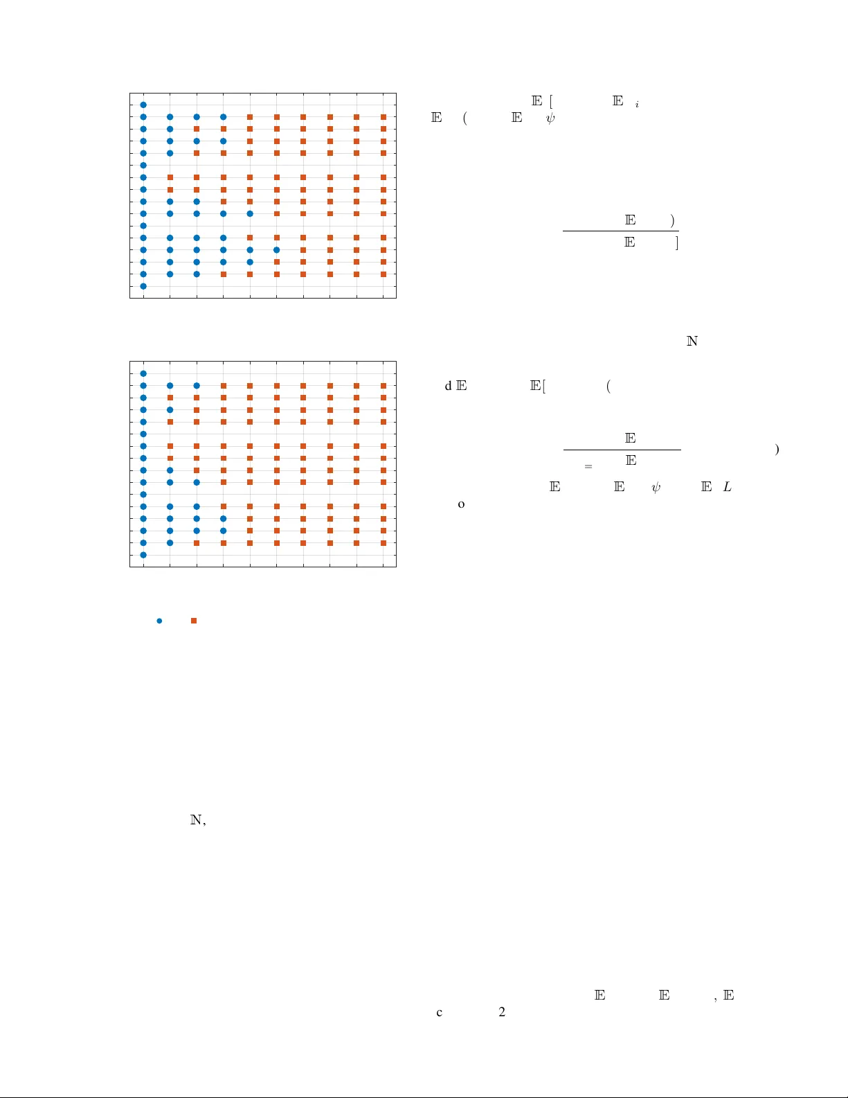
A GE OF INCORRECT INFORMA TION FOR GENERIC DISCRETE-TIME MARKO V SOURCES 1 Age of Incorrect Information for Generic Discrete-T ime Mark o v Sources K onstantinos Bountrogiannis, Anthony Ephremides, Panagiotis Tsakalides, Member , IEEE , and George Tzagkarakis Abstract —This work introduces a framework for analyzing the Age of Incorrect Information (AoII) in a real-time monitoring system with a generic discrete-time Markov source. W e study a noisy communication system employing a hybrid automatic repeat request (HARQ) protocol, subject to a transmission rate constraint. The optimization problem is formulated as a constrained Markov decision process (CMDP), and it is shown that there exists an optimal policy that is a randomized mixtur e of two stationary policies. T o ov ercome the intractability of computing the optimal stationary policies, we develop a multiple- threshold policy class where thresholds depend on the source, the recei ver , and the packet count. By establishing a Marko v renewal structure induced by threshold policies, we derive closed-f orm expressions for the long-term av erage AoII and transmission rate. The proposed policy is constructed via a relativ e value iteration algorithm that leverages the thr eshold structure to skip computations, combined with a bisection sear ch to satisfy the rate constraint. T o accommodate scenarios requiring lower computational complexity , we adapt the same technique to produce a simpler single-threshold policy that trades optimality for efficiency . Numerical experiments exhibit that both threshold- based policies outperform periodic scheduling, with the multiple- threshold approach matching the perf ormance of the globally optimal policy . Index T erms —Age of Incorrect Information, Markov decision process, hybrid ARQ, threshold policies, transmission rate con- straint I . I N T RO D U C T I O N R EAL-TIME monitoring of remote data sources plays a central role in the de v elopment of many emerging applications, driv en by recent advancements in communica- tion and sensing technologies. Examples include autonomous driving, real-time video feedback, anomaly detection in critical infrastructures, remote surgery , augmented reality networks, and haptic communications. In such use cases, the timely deliv ery of information is essential, and the Age of Infor- mation (AoI) [1] metric has been introduced and e valuated to assess system performance. Compared to the traditional K onstantinos Bountrogiannis and P anagiotis Tsakalides are with the Depart- ment of Computer Science, Univ ersity of Crete, Heraklion 700 13, Greece, and with the Institute of Computer Science, Foundation for Research and T echnology – Hellas, Heraklion 700 13, Greece E-mail: kbountrogiannis@csd.uoc.gr; tsakalid@csd.uoc.gr Anthony Ephremides is with the Electrical and Computer Engineering Department, Univ ersity of Maryland, College Park, MD 20742 USA E-mail: etony@umd.edu George Tzagkarakis is with the Institute of Computer Science, Foundation for Research and T echnology – Hellas, Heraklion 700 13, Greece E-mail: gtzag@ics.forth.gr This work was supported in part by the European Commission under the frame work of the National Recovery and Resilience Plan Greece 2.0 – NextGenerationEU, Grant T AEDR-0536642 (Smart Cities). delay metrics, AoI measures not only the communication time in the network, but also the time a message spends before being scheduled for submission to the network. As such, AoI measures the freshness of the communicated information and highlights the need to update the monitoring system with more current data to av oid excessi v e aging. Formally , the AoI process δ AoI t is defined as the difference δ AoI t ≜ t − u t , (1) where u t is the generation time of the most recently received message. One limitation of the traditional AoI metric is that it focuses solely on the freshness of information, without accounting for the dynamics of the data source itself. F or e xample, if one source changes rapidly and another changes slo wly , the same communication system may produce samples with the same AoI for both sources. Howe v er , the sample from the fast-changing source may be less relev ant or useful for decision-making, because it is more likely to deviate from the contemporary source state at the time of arriv al. This observ ation prompted the introduction of the Age of Incorrect Information (AoII) metric [2], which is the focus of this work. Unlike traditional AoI, AoII is a content-aware metric that penalizes the duration during which the information at the monitor differs from the source state, i.e., is incorrect, and is weighted by a distortion function. Specifically , let g ( S t , ˆ S t ) denote a distortion function between the source state S t and the estimate at the monitor ˆ S t at time t . Moreover , define the age function a t ≜ t − h t , (2) where h t is the last time instant when g ( X t , ˆ X t ) was zero. The AoII process ∆ t is the product δ t ≜ a t · g ( X t , ˆ X t ) . (3) In our analysis, we employ an indicator distortion function, g ( X t , ˆ X t ) = 1 { X t  = ˆ X t } . (4) Figure 1 illustrates concurrent sample paths of both the AoI and the AoII. The AoII metric has been mostly studied with discrete-time Markov sources, since they offer an analytical advantage. The source models in [3]–[5] are binary symmetric Markov chains. The works [2], [6]–[9] focus on arbitrarily large symmetric Markov models. In [10], the source model is a bird-death Markov chain. An alternativ e formulation is employed in [11], A GE OF INCORRECT INFORMA TION FOR GENERIC DISCRETE-TIME MARKO V SOURCES 2 s 1 d 1 s 2 d 2 0 1 Source 0 1 Monitor s 1 d 1 s 2 d 2 0 1 Distortion s 1 d 1 s 2 d 2 0 2 4 AoI s 1 d 1 s 2 d 2 time-slots 0 2 4 AoI I Fig. 1. Concurrent discrete-time sample paths of the AoI and AoII. A binary source is sampled at slots s i , i = 1 , 2 , and decoded by the receiver at slots d i , i = 1 , 2 , respectively . The distortion is the absolute difference between the source and monitor values. where the source is not modeled directly , b ut a binary Marko v chain is used to model the distortion function. Those works exhibit that AoII-optimal transmission policies in resource- constrained environments commonly admit a threshold struc- ture, a result also typical for the con ventional AoI [12]–[16]. Generic Mark ov sources, i.e., without any pre-specified structure, have limited appearance in the literature. The semi- nal work [17] analyzes the AoII for a generic continuous-time Markov source, proving that the optimal policy in the contin- uous setting is a multiple-threshold policy where thresholds depend on both the source and the estimate at the receiv er . Acknowledging the intractability of the problem, a suboptimal solution is proposed in which the thresholds depend only on the estimate. Recently , a work av ailable in [18] dev elops a similar policy for a discrete-time Marko v source. Notably , multiple-threshold policies have been previously analyzed in the setting of bird-death Markov chains in [10]. Our work in vestigates a noisy communication system that employs a generic discrete-time Marko v source. The trans- mitter and receiver use a hybrid automatic repeat request (HARQ) protocol to correct transmission errors, with the decoder requesting additional transmissions to improve the decoding probability . Additionally , the transmission policy is 1 2 3 4 p 1 , 1 p 1 , 2 p 1 , 3 p 1 , 4 p 2 , 1 p 2 , 2 p 2 , 3 p 2 , 4 p 3 , 1 p 3 , 2 p 3 , 3 p 3 , 4 p 4 , 1 p 4 , 2 p 4 , 3 p 4 , 4 Fig. 2. A generic Markov chain of N = 4 states. subject to a resource constraint on the long-term average transmission rate. The main contrib utions of our work are summarized as follows: • W e study AoII minimization for generic discrete-time Markov sources ov er a noisy HARQ channel under a transmission rate constraint, extending prior works that focus on structured or symmetric models. • The optimization problem is formulated as a constrained Markov decision process (CMDP), and it is shown that there exists an optimal policy that is a randomized mixture of two stationary policies. • T o address the intractability of computing the optimal stationary policies, we de velop a class of multiple- threshold transmission policies, denoted as F ( S, W , r ) , where transmissions are triggered when the AoII exceeds state-dependent thresholds based on the source state, the receiv er estimate, and the packet count. • W e establish a Markov renew al structure induced by threshold policies and deriv e closed-form expressions for the long-term a verage AoII and transmission rate, enabling efficient ev aluation of candidate policies. Lev er- aging the threshold structure, we design an efficient relativ e value iteration (R VI) algorithm combined with a bisection search to approximate the optimal threshold policy . • T o accommodate scenarios with large state spaces or frequent policy refinements, we dev elop single-threshold policies, F (1) , that trade optimality for efficienc y by lifting the dependency on the real-time system parameters except the AoII. A GE OF INCORRECT INFORMA TION FOR GENERIC DISCRETE-TIME MARKO V SOURCES 3 I I . P RO B L E M D E FI N I T I O N A. Communication Model W e consider a discrete-time (slotted) communication model ov er a noisy channel. W e focus on N -ary generic Marko v sources. In this context, the (single-step) transition probability from state i to state j is denoted by p i,j , { i, j } ∈ { 1 , . . . , N } 2 . An example is depicted in Fig. 2 for N = 4 . At each time slot, the transmitter acquires a sample from the source and decides whether to transmit or discard it. The sam- ple to be transmitted is encoded into a packet with a channel coding scheme and communicated through a noisy channel to the receiv er . Upon receiving the packet, the receiv er attempts to decode it. If the decoding is successful, the recei ver notifies the transmitter with an ACK feedback message. Otherwise, it sends a N A CK message to request an additional transmission, and the transmitter decides whether to retransmit or reject the request. The receiv er holds the last successfully decoded value until the following successful decoding. The probability of successful decoding is specified by a non-decreasing function d ( r ) ∈ (0 , 1) , where r is the number of packets at the receiv er for the specific sample. The packet transmission duration is constant and equal to one time slot, whereas the A CK/N A CK packets are instan- taneous. The instantaneous feedback message is a typical assumption in the literature, justified by its limited information content. Lastly , motiv ated by the need to conserve or allocate power and network resources, we impose a constraint on the trans- mission rate. In particular, it is required that the long-term av erage transmission rate, measured in packets per slot, be less than or equal to R ∈ [0 , 1] . B. Optimization Pr oblem The general problem is formulated as an infinite-horizon av erage-cost constrained Markov decision problem (CMDP) denoted by K = ( X , Y , P , C , R ) , where • the state of the system at time t is K t = ( S t , W t , δ t , r t ) ∈ X , where S t ∈ { 1 , . . . , N } denotes the source state, W t ∈ { 1 , . . . , N } denotes the state known by the receiv er , δ t is the AoII, and r t ∈ { 0 , . . . , r max } is the number of packets receiv ed for the current sample transmission. • The actions y t ∈ Y = { 0 , 1 } denote the action at time t , where the action space consists of the wait ( y t = 0 ) and the transmit ( y t = 1 ) actions. • The action-dependent transition probabilities P ( K t +1 | K t , y t ) are summarized in T able I, reflecting the model as described in Sec. II-A. • The cost at state K t = ( S t , W t , δ t , r t ) is equal to the instantaneous AoII C ( K t ) ≜ δ t . • The long-term average number of “transmit” actions is constrained to not exceed R ∈ (0 , 1] . Our goal is to find the transmission policy ψ = { y t } t ≥ 0 that minimizes the long-term av erage AoII while satisfying the transmission rate constraint. The problem can be expressed as a linear programming problem, as follows, Definition 1 (Main Optimization Problem) . Minimize ¯ J ψ ( L 0 ) ≜ lim sup T →∞ 1 T E ψ " T − 1 X t =0 δ t | L 0 # subject to ¯ R ψ ( L 0 ) ≜ lim sup T →∞ 1 T E ψ " T − 1 X t =0 y t | L 0 # ≤ R (6) The constrained problem can be relaxed to its uncon- strained Lagrangian form. Particularly , define the MDP M = ( X , Y , P , C λ ) , which is identical to K , with the exception that the transmission rate constraint is replaced by a transmission penalty λ , integrated into the instantaneous cost C λ ( M t , y t ) ≜ δ t + λy t . Let ψ λ denote the related transmission policy . Definition 2 (Lagrangian Problem) . Minimize ¯ J ψ λ ( M 0 ) ≜ lim T →∞ sup λ ≥ 0 1 T E ψ λ " T − 1 X t =0 δ t + λy t | M 0 # − λR (7) For any fixed v alue of λ , let ψ ∗ λ ≜ argmin ψ ¯ J ψ λ , (8) g λ ≜ min ψ ¯ J ψ λ , (9) denote the λ -optimal Lagrangian policy and the average cost achiev ed thereof, respectiv ely . It is easy to see that M is unichain, i.e., there exists a single recurrent class. Thus, the optimal policy ψ λ can be found by solving the Bellman equations [19, Thm. 6.5.2], g λ + V ( M t ) = min y t { δ t + λy t + X M t +1 P ( M t +1 | M t , y t ) V ( M t +1 ) } , (10) where V ( M t ) is the value function of the state M t . I I I . O P T I M A L P O L I C Y S T RU C T U R E This section discusses an optimal solution of the CMDP K (6) and the difficulties of its computation. The main result is the following theorem. Theorem 1. There e xists an optimal policy ψ ∗ of (6) , which is a randomized mixtur e of two stationary policies ψ λ + and ψ λ − that are both optimal solutions of the Lagrangian MDP (7) with parameters λ + and λ − , r espectively . In particular , λ + ≜ inf { λ ∈ R + : ¯ R ψ λ ≤ R } , (11) λ − ≜ sup { λ ∈ R + : ¯ R ψ λ ≥ R } , (12) wher e ¯ R ψ λ is the transmission rate achieved by ψ . The optimal policy ψ ∗ randomizes between ψ λ + and ψ λ − whenever the induced Markov chain { M t } t ≥ 0 r eaches their common r e g eneration set C ≜ { K = ( s, w , δ, r ) : s = w , δ = 0 , r = 0 } . (13) Upon r eaching C , the policy ψ ∗ selects ψ λ − with pr obability ρ and ψ λ + with pr obability 1 − ρ . The mixing probability is chosen such that the randomized policy has an averag e transmission rate equal to R , and is explicitly defined as ρ ≜ R − ¯ R ψ λ + ¯ R ψ λ − − ¯ R ψ λ + . (14) A GE OF INCORRECT INFORMA TION FOR GENERIC DISCRETE-TIME MARKO V SOURCES 4 P ( S t +1 , W t +1 = W t , δ t +1 = δ t + 1 , r t +1 = 0 | M t , y t = 0) = p S t ,S t +1 ∀ S t +1  = W t P ( S t +1 = W t , W t +1 = W t , δ t +1 = 0 , r t +1 = 0 | M t , y t = 0) = p S t ,W t P ( S t +1 , W t +1 = W t , δ t +1 = δ t + 1 , r t +1 = 0 | M t , y t = 1) = p S t ,S t +1 · (1 − d ( r t )) ∀ S t +1 / ∈ { S t , W t } P ( S t +1 = W t , W t +1 = W t , δ t +1 = 0 , r t +1 = 0 | M t , y t = 1) = p S t ,W t · (1 − d ( r t )) P ( S t +1 = S t , W t +1 = W t , δ t +1 = δ t + 1 , r t +1 = r t + 1 | M t , y t = 1) = p S t ,S t · (1 − d ( r t )) if S t  = W t P ( S t +1 , W t +1 = S t , δ t +1 = δ t + 1 , r t +1 = 0 | M t , y t = 1) = p S t ,S t +1 · d ( r t ) ∀ S t +1  = S t P ( S t +1 = S t , W t +1 = S t , δ t +1 = 0 , r t +1 = 0 | M t , y t = 1) = p S t ,S t · d ( r t ) (5) T ABLE I T H E A CT I O N - D E P E ND E N T CO N D I TI O NA L T R AN S I TI O N P RO BA B I LI T I E S P ( M t +1 | M t , y t ) . Pr oof. The proof is based on [20]. The details can be found in Appendix A. The optimal policy defined in Theorem 1 randomizes be- tween two policies ψ λ + and ψ λ − . The policy-induced Markov chains of those policies form distinct renewal processes shar- ing a common regeneration set C , the analysis of which yields the long-term av erage AoII of the optimal policy ψ ∗ , as follows. For all i ∈ N , define the re generation (stopping) times under the ψ -induced Markov chain, T i +1 ( ψ ) ≜ min { t > T i ( ψ ) : S t = W t | ψ } , (15) where T 0 ( ψ ) is assumed to be the v ery first visit to C . Each interval [ T i ( ψ ) , T i +1 ( ψ )] defines a r e g eneration cycle . Let L i ( ψ ) ≜ T i +1 ( ψ ) − T i ( ψ ) , (16) J i ( ψ ) ≜ T i +1 ( ψ ) − 1 X t = T i ( ψ ) δ t , (17) define the cycle length and the cumulativ e AoII in the i -th cycle, respectively , under ψ . Proposition 1. The long-term averag e AoII of ψ ∗ equals ¯ J ψ ∗ = ρ E [ J ( ψ λ − )] + (1 − ρ ) E [ J ( ψ λ + )] ρ E [ L ( ψ λ − )] + (1 − ρ ) E [ L ( ψ λ + )] . (18) Pr oof. Define the embedded process { Ψ ∗ i } i ≥ 0 , Ψ ∗ i = ( ψ λ − w .p. ρ , ψ λ + w .p. 1 − ρ , (19) indicating which policy is selected at the re generation times T i . The pair sequence { ( L i ( ψ ) , J i ( ψ )) } i ≥ 0 constitutes a renewal- rew ard process. The result follows from the renewal-re w ard theorem. T o make use of Theorem 1, it is necessary to compute ψ λ and ¯ R ψ λ . Howe v er , their computation is not straightforward. Particularly , (a) The traditional path of analyzing the Bellman equa- tions (10) – in the hope of deriving a threshold structure of ψ λ – is very hard due to the joint transitions of the source-receiv er pair . (b) T o compute ¯ R ψ λ in a scalable manner , the underlying MDP needs to possess a tractable structure. The same difficulties are inherited in the computation of E [ J ψ λ ] , E [ L ψ λ ] in (18). Dynamic programming algorithms, such as the Relativ e V alue Iteration (R VI) and Policy Iteration (PI) [19, Chap. 6], although slow , are valuable for approximating λ -optimal policies. W e present such results in Fig. 3 that experimentally illustrate a threshold structure. Hence, although not prov ably optimal, the threshold structure is a sensible assumption for transmission policies. I V . F ( S, W, r ) : T H E C L A S S O F F U L L S PAC E M U LTI P L E - T H R E S H O L D P O L I C I E S Follo wing the analysis and our observ ations in Sec. III, we introduce a construction method that is optimal under the assumption that ψ λ are threshold-based on δ for all λ . In this section, we study the class of stationary multiple-threshold policies F ( S, W, r ) in which the thresholds depend on the source S , the receiv er W , and the packet count r . Formally , Definition 3. F ( S , W , r ) is the class of policies, wher e each ψ ∈ F ( S, W , r ) is a function of the system state M t = ( s, w , δ, r ) such that ψ ( s, w , δ, r ) = ( 0 if δ < n ( s, w , r ) , 1 if δ ≥ n ( s, w , r ) . (20) Exploiting the structure of the policies in F ( S, W, r ) , we can analyze the policy-induced Markov chain to compute ¯ R ψ λ and construct a fast R VI algorithm that approximates ψ λ . Moreov er , the same analysis can be used to compute ¯ J ψ ∗ (18). A. Analysis of F ( S, W, r ) Consider the Markov chain induced by ψ ∈ F ( S, W, r ) , with the state at time t denoted by H ( ψ ) t = ( S t , W t , δ t , r t ) ∈ X . W e will analyze { H ( ψ ) t } t ≥ 0 into cycles . Each cycle starts and ends in a regeneration state ( S , W , δ, r ) ∈ C (13), i.e., ev ery state with zero AoII. T o characterize each cycle, we will adopt the definitions in (15),(16),(17) to denote the regeneration times T i ( ψ ) , the cycle lengths L i ( ψ ) , and the A GE OF INCORRECT INFORMA TION FOR GENERIC DISCRETE-TIME MARKO V SOURCES 5 0 1 2 3 4 5 6 7 8 9 / (1,1) (1,2) (1,3) (1,4) (2,1) (2,2) (2,3) (2,4) (3,1) (3,2) (3,3) (3,4) (4,1) (4,2) (4,3) (4,4) ( S; W ) r = 1 0 1 2 3 4 5 6 7 8 9 / (1,1) (1,2) (1,3) (1,4) (2,1) (2,2) (2,3) (2,4) (3,1) (3,2) (3,3) (3,4) (4,1) (4,2) (4,3) (4,4) ( S; W ) r = 2 Fig. 3. ψ ∗ λ policy ( wait, transmit) for every source-receiv er ( S, W ) pair, and packet count r = 1 (top) and r = 2 (bottom). Note: When S = W , then δ = 0 always. The maximum transmission packet count is r max = 2 , and the probability of successful decoding d ( r ) is 0 . 5 and 0 . 75 for r = 1 and r = 2 , respectiv ely . The transmission penalty λ = 8 , while the source transition probabilities p i,j are giv en by the transition matrix   0 . 52 0 . 12 0 . 18 0 . 18 0 . 17 0 . 57 0 . 17 0 . 09 0 . 03 0 . 06 0 . 72 0 . 19 0 . 16 0 . 10 0 . 18 0 . 56   . cumulativ e AoII J i ( ψ ) in the i -th cycle, respectiv ely , under ψ . Notice that every state ( S, W, δ, r ) ∈ C can be written as ( S, S, 0 , 0) , and is thereby distinguishable by the source value S . For all i ∈ N , define the embedded Markov chain { Z i ( ψ ) } i ≥ 0 that tracks the regeneration states of { H ( ψ ) t } t ≥ 0 , Z i ( ψ ) = S T i ( ψ ) . (21) W ithin each cycle, the AoII starts from zero and grows linearly until the end of the cycle. This allows writing J i ( ψ ) with the following alternati ve expression that is free of the δ t parameter , J i ( ψ ) = L i ( ψ ) − 1 X n =0 n . (22) The sequence { ( Z i ( ψ ) , L i ( ψ )) } i ≥ 0 forms a Markov renewal process [21]. Let Z denote the state space of { Z i ( ψ ) } i ≥ 0 . For all z ∈ Z , we employ the following conditional expec- tation notations, E z [ J ( ψ )] ≜ E [ J i ( ψ ) | Z i ( ψ ) = z ] and E z [ L ( ψ )] ≜ E [ L i ( ψ ) | Z i ( ψ ) = z ] . In addition, let π z | ψ denote the steady-state probability mass function of Z i ( ψ ) . The follo wing corollary is an application of the renewal-re w ard theorem. Corollary 1. The long-term averag e AoII equals ¯ J ψ = P N z =1 π z | ψ E z [ J ( ψ )] P N z =1 π z | ψ E z [ L ( ψ )] . (23) Follo wing the same procedure, we can characterize the long-term av erage transmission rate. Define the number of transmissions in the i -th cycle, C i ( ψ ) ≜ T i +1 ( ψ ) − 1 X t = T i ( ψ ) y t , ∀ i ∈ N , (24) and E z [ C ( ψ )] ≜ E [ C i ( ψ ) | Z i ( ψ ) = z ] as previously . Corollary 2. The long-term avera ge tr ansmission rate equals ¯ R ψ = P N z =1 π z | ψ E z [ C ( ψ )] P N z =1 π z | ψ E z [ L ( ψ )] , (25) T o compute π z | ψ , E z [ J ( ψ )] , E z [ C ( ψ )] , and E z [ L ( ψ )] , we rely on the theory of absorbing Markov chains [22, Chap. 3]. Let { H ( ψ ) ∗ t } be an augmented Markov chain that mimics the transitions of { H ( ψ ) t } , but is also equipped with absorbing states that correspond to the regeneration states of { H ( ψ ) t } . The transition matrix of { H ( ψ ) ∗ t } is constructed as follows. Denote with Q ( ψ ) the transient-to-transient probability ma- trix, and with U ( ψ ) the transient-to-absorbing probability matrix. As noted above, the ending state of the i -th cycle can be represented solely by the source state S T i +1 ( ψ ) = Z i +1 ( ψ ) , simplifying the dimensionality of U ( ψ ) . Thus, Q ( ψ ) ( S,W ,δ,r ) , ( S ′ ,W ′ ,δ ′ ,r ′ ) denotes the probability that the aug- mented chain transits from the transient state ( S, W, δ, r ) to another transient state ( S ′ , W ′ , δ ′ , r ′ ) , while U ( ψ ) ( S,W ,δ,r ) , ( Z ) de- notes the transition probability to the regeneration (absorbing) state Z ∈ Z = { 1 , . . . , N } . The state space of { H ( ψ ) ∗ t } is H ∗ = X ∪ Z . Clearly , a cycle in { H ( ψ ) t } corresponds to a path in { H ( ψ ) ∗ t } starting from the same state and ending in some absorbing state. It is important to note that all states in the state space of { H ( ψ ) t } are considered as starting states in the construction of Q ( ψ ) ; ev en the regeneration states, since they are the starting points of ev ery cycle. Concurrently , U ( ψ ) encodes the probability to arrive at some regeneration state. Notice that the AoII is unbounded, which leads to infinite- sized matrices Q ( ψ ) and U ( ψ ) . Fortunately , the AoII dimen- sion can be truncated without loss of information. T o see this, observe that the transition probabilities do not depend explicitly on the precise v alue of δ t , but only whether δ t lies below or abov e the corresponding threshold. The same holds for the computation of E z [ L ( ψ )] , E z [ J ( ψ )] , E z [ C ( ψ )] (cf. (16), (22), (24)). Therefore, the AoII dimension can be truncated at the maximum threshold value n max ≜ A GE OF INCORRECT INFORMA TION FOR GENERIC DISCRETE-TIME MARKO V SOURCES 6 max { s,w,r } n ( s, w , r ) . More precisely , let ˜ δ t denote the AoII index in the truncated space. Then, ˜ δ t ≜ min( δ t , n max ) , (26) which preserves the transition structure and all performance metrics of interest while yielding finite-dimensional matrices Q ( ψ ) and U ( ψ ) . W ith the abov e notes at hand, Q ( ψ ) and U ( ψ ) satisfy Q ( ψ ) ( S,W , ˜ δ ,r ) , ( S ′ ,W ′ , ˜ δ ′ ,r ′ ) = ( P ( S ′ ,W ′ , ˜ δ ′ ,r ′ | S,W , ˜ δ ,r ) if ˜ δ ′ > 0 , 0 if ˜ δ ′ = 0 . (27) U ( ψ ) ( S,W , ˜ δ ,r ) , ( Z ) = ( P ( Z, Z , ˜ δ ′ , r ′ | S, W , ˜ δ , r ) if ˜ δ ′ = 0 , 0 if ˜ δ ′ > 0 . (28) The complete transition matrix of { H ( ψ ) ∗ t } is P H ( ψ ) ∗ ≜  Q ( ψ ) U ( ψ ) 0 I  . (29) In the context of absorbing Markov chains, the fundamental matrix N ( ψ ) ≜ ( I − Q ( ψ ) ) − 1 quantifies the expected number of visits in every transient state until absorption. More precisely , N ( ψ ) ( S,W , ˜ δ ,r ) , ( S ′ ,W ′ , ˜ δ ′ ,r ′ ) is the expected number of visits in the state ( S ′ , W ′ , ˜ δ ′ , r ′ ) before absorption, when starting from the state ( S, W, δ, r ) . In addition, the absorption probability matrix B ( ψ ) ≜ N ( ψ ) · U ( ψ ) represents the probabilities of being absorbed into each state. Theorem 2. The statistical parameter s of the ψ -induced system, ψ ∈ F ( S, W, r ) , ar e computed as follows. E z [ L ( ψ )] = m ( ψ ) ( z ,z, 0 , 0) , (30) E z [ J ( ψ )] = u ( ψ ) ( z ,z, 0 , 0) − m ( ψ ) ( z ,z, 0 , 0) 2 , (31) E z [ C ( ψ )] = X ( S ′ ,W ′ , ˜ δ ′ ,r ′ ) : ˜ δ ′ = n ( S ′ ) − 1 ρ ( S ′ ) N ( ψ ) ( z ,z, 0 , 0) , ( S ′ ,W ′ , ˜ δ ′ ,r ′ ) (32) + X ( S ′ ,W ′ , ˜ δ ′ ,r ′ ) : ˜ δ ′ ≥ n ( S ′ ) N ( ψ ) ( z ,z, 0 , 0) , ( S ′ ,W ′ , ˜ δ ′ ,r ′ ) , (33) wher e the vectors m ( ψ ) = N ( ψ ) 1 , u ( ψ ) = N ( ψ ) ( 1 + 2 Q ( ψ ) N ( ψ ) 1 ) , 1 ≜ [1 1 · · · 1] T . Mor eover , the steady-state mass function π z | ψ can be derived accor ding to the transition pr obability matrix of { Z i } , which equals P z ,z ′ | ψ = B ( ψ ) ( z ,z, 0 , 0) , ( z ′ ) . Pr oof. T o prove the result, we analyze { H ( ψ ) ∗ t } exploiting its absorbing structure. W e deri ve the expressions by character- izing the time to absorption as a function of the initial state. The details can be found in Appendix B. Theorem 2 provides the necessary material to compute the closed-form expressions of the long-term a verage AoII J ψ (23) and transmission rate ¯ R ψ (25). W e conclude this section with the following useful result. Proposition 2. The optimal action at states with zer o AoII, i.e., ( s, s, 0 , 0) for all s ∈ { 1 , . . . , N } , is to wait ( y = 0 ). Pr oof. W e utilize the R VI algorithm and show that at every iteration, the action that minimizes the value function is y = 0 . Since R VI con ver ges to the true v alue function, it follows that the optimal action is also y = 0 . The proof is detailed in Appendix D. A direct consequence of the above is the following. Corollary 3. The optimal thr esholds satisfy n ( s, w , r ) > 0 for all s ∈ { 1 , . . . , N } , w ∈ { 1 , . . . , N } , r ∈ { 1 , . . . , r max } . B. Appr oximation of F ( S , W , r ) The threshold structure of F ( S, W, r ) can be exploited to reduce the complexity of dynamic programming algorithms, omitting computations for the states with δ above the current threshold. It is important to note that the state space of the Lagrangian MDP is infinite because the AoII is unbounded, rendering dynamic programming algorithms intractable. T o address this issue, we adopt the Approximating Sequence Method [23]. That is, truncate the state space by limiting the AoII component to at most ∆ . The truncated MDP is constructed by replacing the transitions ( s, w , ∆ , r ) → ( s ′ , w ′ , ∆ + 1 , r ′ ) by ( s, w , ∆ , r ) → ( s ′ , w ′ , ∆ , r ′ ) . Let the resulting MDP and its optimal average cost be denoted by M (∆) λ and g (∆) λ , respectiv ely . Theorem 3. Let e (∆) r ealize the optimal policy of M (∆) λ . Then, i) The limit point of e (∆) is optimal for M λ . ii) lim ∆ →∞ g (∆) λ = g λ . Pr oof. W e verify Assumptions 1-2 in [23]. Then, Theorem 2.2 of the same reference is applied to prove the result. The details can be found in Appendix C. From Theorem 3, we infer that for sufficiently large ∆ , the approximation on the truncated MDP will be adequately close to the true optimal policy . An R VI algorithm that realizes this approximation is shown in Alg. 1 in Appendix E. C. Appr oximation of the Optimal P olicy ψ ∗ Giv en the abov e results, the optimal policy can be con- structed via a bisection search, whose computational complex- ity is at the order of O (log λ + ) [24]. The algorithm adopted in this paper is an adaptation of [10, Alg. 2]. The pseudocode is giv en in Alg. 2 in Appendix E. V . F (1) : T H E C L A S S O F S I N G L E - T H R E S H O L D P O L I C I E S The previous section addressed the construction of general multiple-threshold policies that depend on all system param- eters. The construction of these policies relies on an efficient A GE OF INCORRECT INFORMA TION FOR GENERIC DISCRETE-TIME MARKO V SOURCES 7 F ( S , W , r ) ( δ max ) 6 9 8 7 ( δ max ) 8 6 3 3 ( δ max ) 5 7 5 8 ( δ max ) F (1) 8 8 8 8 Fig. 4. The stationary threshold policy component ψ λ + of the randomized policy ψ ∗ for each of the threshold policy classes introduced in the previous sections. For the policy in F ( S, W, r ) , only the thresholds for packet count r = 1 are shown. The transmission rate is R = 0 . 1 , the maximum transmission packet count is r max = 2 , and the probability of successful decoding d ( r ) is 0 . 5 and 0 . 75 for r = 1 and r = 2 , respectively . The source transition probabilities p i,j are given by the transition matrix   0 . 52 0 . 12 0 . 18 0 . 18 0 . 17 0 . 57 0 . 17 0 . 09 0 . 03 0 . 06 0 . 72 0 . 19 0 . 16 0 . 10 0 . 18 0 . 56   . R VI algorithm that le verages the threshold structure to skip computations. Howe ver , the state space is still large, with a state space of size |X | = N 2 · ∆ · r max . Moreover , each Bell- man ev aluation requires O ( N ) operations, scaling the worst- case complexity of the R VI algorithm into O ( N 3 · ∆ · r max ) . In this section, we introduce F (1) , the class of single- threshold policies that apply the same threshold e verywhere. Therein, the state space scales linearly with N , yielding a worst-case R VI complexity of O ( N 2 · ∆ · r max ) . Notably , the bisection method can directly search for the threshold n with- out employing R VI, thereby offering a substantial reduction in complexity . Definition 4. F (1) is the class of policies, wher e each ψ ∈ F (1) is a thr eshold function of the AoII δ , ψ ( δ ) = ( 0 if δ < n, 1 if δ ≥ n. (34) Since F (1) is a special case of F ( S, W, r ) , the results of Sec. IV -A hold. Specifically , Corollaries 1-2 and Theorem 2 enable the computation of the long-term a verage AoII and transmission rate of any policy ψ ∈ F (1) . T o simplify notation, let R n equal the long-term av erage transmission rate R ψ when ψ ∈ F (1) with threshold n . Algorithm 3 in Appendix E summarizes the search algorithm. V I . N U M E R I C A L R E S U LT S Figure 4 illustrates the approximated policies of F ( S, W, r ) and F (1) , for the same source model as in Fig. 3 and transmission rate R = 0 . 1 . Hereafter , each experiment is carried out on a distinct, randomly drawn Markov source. For the experiments to be informativ e, we bias the diagonal elements of P to be the largest element in its row . Otherwise, there is a high probability that the selected Markov source contains multiple states where transmissions are ne ver preferable, making the comparison across the different source models complex. In practice, this assumption implies that the duration of a transmission (one time slot) is shorter than the av erage time required for the source to change value. In our e xperiments, each row possesses 0.1 0.2 0.3 0.4 0.5 T ransmission rate 2 2.5 3 3.5 Av erage AoI I F ( S; W; r ) F (1) Periodic Optimal Fig. 5. A v erage AoII versus transmission rate for a random source - N = 4 0.1 0.2 0.3 0.4 0.5 T ransmission rate 4 4.5 5 5.5 6 6.5 7 7.5 8 Av erage AoI I F ( S; W; r ) F (1) Periodic Optimal Fig. 6. A v erage AoII versus transmission rate for a random source - N = 8 0.1 0.2 0.3 0.4 0.5 T ransmission rate 10 11 12 13 14 15 16 Av erage AoI I F ( S; W; r ) F (1) Periodic Optimal Fig. 7. A verage AoII versus transmission rate for a random source - N = 16 A GE OF INCORRECT INFORMA TION FOR GENERIC DISCRETE-TIME MARKO V SOURCES 8 N elements that are uniformly distributed and normalized, and the diagonal element is assigned the largest of those elements. Similar to [12] and [6], the probability of failed decoding is modeled as an exponentially decreasing function, i.e., p ( r ) = 1 − p e c r , for 0 ≤ r ≤ r max , (35) where p e is the initial error rate and c ∈ (0 , 1] is the decaying error rate constant. T o facilitate comparison of the transmission policies, the chosen parameters are constant at c = 0 . 5 , p e = 0 . 5 , and r max = 2 . Figures 5 - 7 illustrate the average AoII achiev ed by the proposed policies versus the transmission rate, together with the AoII of the optimal policy without the constraint of the threshold structure. Additionally , results are drawn for a periodic policy that transmits e very ⌈ 1 /R ⌉ time slots. Each figure is dedicated to a different cardinality , N = 4 , 8 , 16 . Our results confirm that searching within the F ( S, W, r ) threshold class incurs no loss of optimality , as its performance perfectly matches the globally optimal policy . This approach yields strict improv ements over all alternati ves, especially in the lower transmission-rate region. Finally , we observe that ev en the elementary single-threshold policy F (1) dramatically outperforms periodic transmissions. V I I . C O N C L U S I O N This work inv estigates transmission policies for minimizing the AoII metric of generic discrete-time Markov sources. The considered communication model employs an HARQ protocol for error correction under a constrained transmission rate. W e demonstrate that the optimization problem can be formulated as a CMDP , and that there exists an optimal policy which is a randomized mixture of two stationary policies. W e propose a method for deriving feasible multiple-threshold policies, where transmissions occur as long as the AoII is larger than state-dependent thresholds that rely on the source, receiv er , and packet count. The resulting system is analyzed as a Marko v rene wal process, allowing for the deri v ation of closed-form expressions for both the long-term average AoII and the av erage transmission rate. The threshold allocation is carried out via a relativ e v alue iteration algorithm acting on a truncated state space, paired with a bisection search to approximate the optimal transmission penalty . For reduced complexity , a simpler single-threshold policy can be deri ved that significantly scales down the state space. The results demonstrate the superiority of threshold-based policies over con v entional periodic transmission schemes and highlight the potential of multiple-threshold policies in AoII optimization problems. R E F E R E N C E S [1] S. Kaul, R. Y ates, and M. Gruteser , “Real-time status: How often should one update?” in 2012 Pr oceedings IEEE INFOCOM , 2012, pp. 2731– 2735. [2] A. Maatouk, S. Kriouile, M. Assaad, and A. Ephremides, “The age of incorrect information: A new performance metric for status updates, ” IEEE/ACM T ransactions on Networking , vol. 28, no. 5, pp. 2215–2228, 2020. [3] C. Kam, S. Kompella, and A. Ephremides, “ Age of incorrect information for remote estimation of a binary markov source, ” in IEEE INFOCOM 2020 - IEEE Conference on Computer Communications W orkshops (INFOCOM WKSHPS) , 2020, pp. 1–6. [4] Y . Chen and A. Ephremides, “Preempting to minimize age of incorrect information under transmission delay , ” IEEE T ransactions on Network- ing , pp. 1–13, 2025. [5] ——, “ Analysis of age of incorrect information under generic transmis- sion delay , ” in IEEE INFOCOM 2023 - IEEE Conference on Computer Communications W orkshops (INFOCOM WKSHPS) , 2023, pp. 1–8. [6] K. Bountrogiannis, A. Ephremides, P . Tsakalides, and G. Tzagkarakis, “ Age of incorrect information with hybrid arq under a resource con- straint for n -ary symmetric markov sources, ” IEEE Tr ansactions on Networking , pp. 1–14, 2024. [7] S. Kriouile and M. Assaad, “Minimizing the age of incorrect information for real-time tracking of markov remote sources, ” in 2021 IEEE Interna- tional Symposium on Information Theory (ISIT) , 2021, pp. 2978–2983. [8] K. Bountrogiannis, I. Papoutsidakis, A. Ephremides, P . Tsakalides, and G. Tzagkarakis, “V ariable-length stop-feedback coding for minimum age of incorrect information, ” in Pr oceedings of the T wenty-Fifth International Symposium on Theory, Algorithmic F oundations, and Pr otocol Design for Mobile Networks and Mobile Computing , ser. MobiHoc ’24. Ne w Y ork, NY , USA: Association for Computing Machinery , 2024, p. 410–415. [Online]. A vailable: https://doi.org/10. 1145/3641512.3690165 [9] S. Kriouile and M. Assaad, “Minimizing the age of incorrect information for unknown marko vian source, ” 2022. [Online]. A vailable: https://arxiv .org/abs/2210.09681 [10] Y . Chen and A. Ephremides, “Minimizing age of incorrect information for unreliable channel with power constraint, ” in 2021 IEEE Global Communications Confer ence (GLOBECOM) , 2021, pp. 1–6. [11] A. Maatouk, M. Assaad, and A. Ephremides, “The age of incorrect information: an enabler of semantics-empo wered communication, ” IEEE T r ansactions on W ir eless Communications , pp. 1–1, 2022. [12] E. T . Ceran, D. G ¨ und ¨ uz, and A. Gy ¨ orgy , “ A verage age of information with hybrid ARQ under a resource constraint, ” IEEE T ransactions on W ir eless Communications , vol. 18, no. 3, pp. 1900–1913, 2019. [13] A. Arafa, J. Y ang, S. Ulukus, and H. V . Poor , “ Age-minimal transmission for ener gy harvesting sensors with finite batteries: Online policies, ” IEEE T r ansactions on Information Theory , vol. 66, no. 1, pp. 534–556, 2020. [14] B. T . Bacinoglu, Y . Sun, E. Uysal, and V . Mutlu, “Optimal status updating with a finite-battery energy harvesting source, ” Journal of Communications and Networks , vol. 21, no. 3, pp. 280–294, 2019. [15] X. W u, J. Y ang, and J. W u, “Optimal status update for age of information minimization with an energy harvesting source, ” IEEE Tr ansactions on Gr een Communications and Networking , v ol. 2, no. 1, pp. 193–204, 2018. [16] Y . Sun and B. Cyr , “Sampling for data freshness optimization: Non- linear age functions, ” J ournal of Communications and Networks , vol. 21, no. 3, pp. 204–219, 2019. [17] I. Cosandal, N. Akar , and S. Ulukus, “Multi-threshold aoii-optimum sampling policies for continuous-time marko v chain information sources, ” IEEE T ransactions on Information Theory , pp. 1–1, 2025. [18] I. Cosandal, S. Ulukus, and N. Akar , “Minimizing functions of age of incorrect information for remote estimation, ” 2025. [Online]. A v ailable: https://arxiv .org/abs/2504.10451 [19] V . Krishnamurthy , P artially Observed Markov Decision Pr ocesses: F rom F iltering to Contr olled Sensing . Cambridge University Press, 2016. [20] L. I. Sennott, “Constrained av erage cost Markov decision chains, ” Pr obability in the Engineering and Informational Sciences , vol. 7, no. 1, pp. 69–83, 1993. [21] E. Cinlar , Intr oduction to Stochastic Processes . Dover Publications, 2013. [22] J. G. Kemen y and J. L. Snell, F inite markov chains . van Nostrand Princeton, NJ, 1969, vol. 26. [23] L. I. Sennott, “On computing average cost optimal policies with applica- tion to routing to parallel queues, ” Mathematical methods of operations r esear ch , vol. 45, no. 1, pp. 45–62, 1997. [24] T . H. Cormen, C. E. Leiserson, R. L. Riv est, and C. Stein, Introduction to Algorithms, Third Edition , 3rd ed. The MIT Press, 2009. A GE OF INCORRECT INFORMA TION FOR GENERIC DISCRETE-TIME MARKO V SOURCES 9 A P P E N D I X A. Pr oof of Theor em 1 Pr oof. First, we prov e that assumptions 1-5 of [20] hold for our problem. Under those properties, the results of [20] yield the existence and structure of an optimal policy . Definition 5 (Definition 2.3 of [20]) . Let G ⊂ M be a non- empty subset of states of the CMDP . Given a state m ∈ M , let R ( m, G ) be the class of policies ψ such that P ψ ( M t ∈ G for some t ≥ 1 | M 0 = m ) = 1 and the expected time T m,G of the first passage fr om m to G under ψ is finite. Let R ∗ ( m, G ) be the class of policies ψ ∈ R ( m, G ) such that, in addition, the expected avera ge AoII ¯ J m,G ( ψ ) and the expected transmission rate ¯ R m,G ( ψ ) of the first passage fr om m to G ar e finite. Hereafter , we state and prove the assumptions mentioned abov e for our problem. Assumption 1. F or all b > 0 , the set G ( b ) ≜ { M = ( s, w , δ, r ) | ther e exists an action y such that δ + y ≤ b } is finite. Pr oof. Since δ ∈ N , the states with δ < w are always finite, which implies that G ( b ) is also finite. Assumption 2. Ther e exists a stationary policy e that induces a Markov chain with the following pr operties: the state space M consists of a single (non-empty) positive recurr ent class K and a set U of transient states such that e ∈ R ∗ ( u, K ) , for any u ∈ U . Moreo ver , both the averag e AoII ¯ J e and the averag e transmission rate ¯ R e on K ar e finite. Pr oof. Consider the policy e ( m ) = 0 for all m ∈ M , i.e., the always-wait policy . Let m 0 = ( s 0 , w 0 , δ 0 , r 0 ) . It can be seen that the policy-induced Marko v chain { M e ( t ) } = { s t , w t , δ t , r t } , t ∈ N has a single positive recurrent class K ψ = { ( s, w , δ, r ) : s ∈ { 1 , . . . , N } , w = w 0 , δ ∈ N , r = 0 } . The transient set is U = { ( s, w , δ, r ) : s ∈ { 1 , . . . , N } , w = w 0 , δ ∈ N , r > 0 } , i.e., they dif ferentiate only on the r component. Recall that the wait action always reverts r to zero, which implies that the expected time of the first passage T u,K ≤ 1 . In addition, the expected transmission rate of the first passage ¯ R u,K ( e ) = 0 , while the expected average AoII of the first passage ¯ J u,K ( e ) is tri vially finite. Hence, e ∈ R ∗ ( u, K ) . In addition, the av erage transmission rate ¯ R e = 0 . T o show that ¯ J e is finite, notice that the AoII δ t rev erts to zero when s t = w 0 , and grows linearly otherwise. W e infer that the Markov chain forms a renew al process wherein the regenera- tion (stopping) times are χ i +1 ≜ inf { t > χ i : s t = w 0 } and the cycle lengths µ i ≜ χ i +1 − χ i . Therefore, the cumulati ve AoII in the i -th cycle equals g i = µ i − 1 X n =0 n = µ 2 i − µ i 2 . (36) Hence, E [ g ] = E [ µ 2 ] − E [ µ ] 2 . (37) By the renew al-re ward theorem, ¯ J e ( m 0 ) = E [ g ] E [ µ ] = E [ µ 2 ] − E [ µ ] 2 E [ µ ] . (38) Recall that the source Markov chain { S t } is finite and irre- ducible, which implies that E [ µ 2 ] < ∞ . Therefore, ¯ J e ( m 0 ) < ∞ . Assumption 3. Given any two states m  = m ′ ∈ M , there exists a policy ψ (a function of m and m ′ ) such that ψ ∈ R ∗ ( m, m ′ ) . Pr oof. Again, consider the policy ψ ( m ) = 1 for all m ∈ M , and recall that the induced Markov chain consists of a single positiv e recurrent class that is e xactly the state space M . Thus, any two states communicate. The average AoII and the transmission rate of the first passage are trivially finite, i.e., ψ ∈ R ∗ ( m, m ′ ) . Assumption 4. If a deterministic policy f has at least one positive r ecurr ent state, then it has a single positive r ecurr ent class K . Moreover , if m 0 / ∈ K , then ψ ∈ R ∗ ( m 0 , K ) . Pr oof. If f transmits for all source states, then there exists a single positiv e recurrent class K = M and the state m 0 is always in K . Assume that f never transmits for some subset of the source states S I ⊂ { 1 , . . . , N } . Denote the complement set with S T . Then, the induced Markov chain consists of a single positiv e recurrent K = { ( s, w , δ, r ) : s ∈ { 1 , . . . , N } , w ∈ S T , δ ∈ N , r ∈ { 1 , . . . , r max }} . Let m 0 = ( s 0 , w 0 , δ 0 , r 0 ) / ∈ K . The source state s 0 communicates with S T . Therefore, f is bound to transmit some source state from S T in finite time, and the receiv er is bound to decode one in finite time. At this time, the chain reaches the class K . Assumption 5. There e xists a policy ψ such that ¯ J ψ ( m 0 ) < ∞ and ¯ R ψ ( m 0 ) < R . Pr oof. This is shown in the proof of Assumption 3. Having prov en assumptions 1-5, the results [20, Thm. 2.5, Prop. 3.2, Lemmas 3.4, 3.7, 3.9, 3.10, 3.12] also hold for our CMDP . By definition, λ − and λ + con v erge to the same λ ∗ from below and above, respecti v ely . By [20, Lemma 3.4, Lemma 3.7], the policies ψ λ − and ψ λ + also conv erge and have the same cost g λ ∗ . Since C (13) is positive recurrent for both policies, a randomized policy that randomizes at C is also λ ∗ -optimal [20, Lemma 3.9]. Finally , applying [20, Lemmas 3.10, 3.12], the optimality of the randomized policy ψ ∗ for the CMDP is deduced. B. Pr oof of Theor em 2 Pr oof. T o simplify the notation throughout this proof, we omit the policy ψ from the notation. All quantities below are understood to depend on ψ . Let τ H ∗ t denote the time until absorption starting from the state H ∗ t . More precisely , τ H ∗ t ≜ min { n ≥ t : H ∗ n ∈ Z , n > t } − t . (39) A GE OF INCORRECT INFORMA TION FOR GENERIC DISCRETE-TIME MARKO V SOURCES 10 Clearly , L i = τ H ∗ T i , ∀ i ∈ N . (40) Assume that H ∗ t is a transient state, as is the case with cycle-starting states. First-step conditioning of τ ( H ∗ t ) yields τ H ∗ t = 1 + τ H ∗ t +1 (41) ⇒ τ 2 H ∗ t = 1 + 2 τ H ∗ t +1 + τ 2 H ∗ t +1 . (42) Let E h ∗ [ τ ] ≜ E [ τ H ∗ t | H ∗ t = h ∗ ] and E h ∗ [ τ 2 ] ≜ E [ τ 2 H ∗ t | H ∗ t = h ∗ ] , h ∗ ∈ H ∗ . T aking the conditional expectation on either sides of (41) and (42) returns the following. E [ τ H ∗ t | H ∗ t = h ∗ ] = 1 + E [ τ H ∗ t +1 | H ∗ t = h ∗ ] ⇒ E h ∗ [ τ ] = 1 + X h ′ ∈H ∗ Q h ∗ ,h ′ E h ′ [ τ ] , (43) E [ τ 2 H ∗ t | H ∗ t = h ∗ ] = 1 + 2 E [ τ H ∗ t +1 | H ∗ t = h ∗ ] + E [ τ 2 H ∗ t +1 | H ∗ t = h ∗ ] ⇒ E h ∗ [ τ 2 ] = 1 + 2 X h ′ ∈H ∗ Q h ∗ ,h ′ E h ∗ [ τ ] + X h ′ ∈H ∗ Q h ∗ ,h ′ E h ∗ [ τ 2 ] . (44) Define the column vectors m and v with elements m h ∗ ≜ E h ∗ [ τ ] and v h ∗ ≜ E h ∗ [ τ 2 ] , respectively . In addition, define the column vector 1 ≜ [1 1 · · · 1] T . Then, (43) and (44) can be written more concisely in matrix-vector form as, m = 1 + Qm ⇒ m = ( I − Q ) − 1 1 ⇒ m = N 1 , (45) u = 1 + 2 Qm + Qu ⇒ u = ( I − Q ) − 1 ( 1 + 2 Qm ) ⇒ u = N ( 1 + 2 QN 1 ) . (46) First, it can be seen that E z [ L ] = m ( z ,z, 0 , 0) . (47) Moreov er , E z [ J ] = E   T i +1 − T i − 1 X k =0 k       Z i = z   = E  ( T i +1 − T i ) 2 − ( T i +1 − T i ) 2     Z i = z  = E  L 2 i − L i 2     Z i = z  = E [ L 2 i | Z i = z ] − E [ L i | Z i = z ] 2 = E ( z ,z, 0 , 0) [ τ 2 ] − E ( z ,z, 0 , 0) [ τ ] 2 = u ( z ,z, 0 , 0) − m ( z ,z, 0 , 0) 2 . (48) T o compute E z [ C ] , we inv oke the expectation of (20) ov er the visited states until absorption, starting from the state ( z , z , 0 , 0) . Since N ( z ,z, 0 , 0) , ( S ′ ,W ′ , ˜ δ ′ ,r ′ ) is the av erage number of visits in ( S ′ , W ′ , ˜ δ ′ , r ′ ) before absorption, it follows that E z [ C ] = E   T i +1 − 1 X t = T i y t       Z i = z   = E   X ( S ′ ,W ′ , ˜ δ ′ ,r ′ ) ψ ( S ′ , ˜ δ ′ , r ′ ) N ( z ,z, 0 , 0) , ( S ′ ,W ′ , ˜ δ ′ ,r ′ )   = X ( S ′ ,W ′ , ˜ δ ′ ,r ′ ) E h ψ ( S ′ , ˜ δ ′ , r ′ ) i N ( z ,z, 0 , 0) , ( S ′ ,W ′ , ˜ δ ′ ,r ′ ) = X ( S ′ ,W ′ , ˜ δ ′ ,r ′ ) P  ψ ( S ′ , ˜ δ ′ , r ′ ) = 1  N ( z ,z, 0 , 0) , ( S ′ ,W ′ , ˜ δ ′ ,r ′ ) = X ( S ′ ,W ′ , ˜ δ ′ ,r ′ ) : ˜ δ ′ = n ( S ′ ) − 1 ρ ( S ′ ) N ( z ,z, 0 , 0) , ( S ′ ,W ′ , ˜ δ ′ ,r ′ ) + X ( S ′ ,W ′ , ˜ δ ′ ,r ′ ) : ˜ δ ′ ≥ n ( S ′ ) N ( z ,z, 0 , 0) , ( S ′ ,W ′ , ˜ δ ′ ,r ′ ) . (49) Now , assume that Z i +1 = z is the ending (absorbing) state of the i -th cycle. Then, the starting state of the next is H T i +1 = ( z , z , 0 , 0) . Let P Z denote the transition matrix of { Z i } . It follows that P Z can be constructed as P Z z ,z ′ = B ( z ,z, 0 , 0) , ( z ′ ) . (50) C. Pr oof of Theor em 2 Pr oof. The result follows from [23, Thm. 2.2], by which it sufficed to sho w that the assumptions [23, ASM 1, ASM 2] hold for our problem. Before proving the assumptions, we define some necessary quantities. For this proof, the quantities in M (∆) are super- scripted by ∆ , and the components of m are denoted by m ( s ) , m ( w ) , m ( δ ) , m ( r ) . Let θ be an arbitrary policy . For a discount factor a , the total expected discounted cost under θ is giv en by V θ,a ( m ) = E θ " ∞ X t =0 a t ( δ t + λy t )      M 0 = m # . (51) The v alue function V a ( · ) = inf θ V θ,a ( m ) is the best that can be achiev ed. The minimum expected discounted cost for operating the system from time t = 0 to t = n − 1 is giv en by v a,n ( m ) = inf θ E θ " n − 1 X t =0 a t ( δ t + λy t )      M 0 = m # , (52) which is also written in recursiv e form as v a,n +1 ( m ) = min y ( m ( δ ) + λm ( y ) + a X m ′ ∈M P ( m ′ | m, y ) v a,n ( m ′ ) ) , (53) Let h ∆ a ( m ) = V ∆ a ( m ) − V ∆ a ( m ref ) be the relative v alue function in M (∆) , where m ref ∈ X ∆ is some chosen reference state. A GE OF INCORRECT INFORMA TION FOR GENERIC DISCRETE-TIME MARKO V SOURCES 11 Giv en a randomized stationary policy ψ of M , the ∆ - restriction of ψ is the randomized stationary policy ψ | ∆ of M (∆) that chooses actions under the same distrib utions as ψ . Let m m,m ref ( ψ | ∆) and c m,m ref ( ψ | ∆) denote the expected time and expected cost, respectiv ely , of the first passage from m to m ref . Giv en initial state m , the average cost under a policy θ is giv en by J θ ( m ) = lim sup T →∞ 1 T E θ " T − 1 X t =0 δ t + λy t      M 0 = m # . (54) Then J ( · ) = inf θ J θ ( · ) is the best that can be achiev ed. The structure of our truncated MDP matches that of augmentation type appr oximating sequences [23, Def. 3.1]. Specifically , let P ( m ′ | m, y ; ∆) denote the action-dependent transition probabilities in M (∆) . Assume that P ( µ | m, y ) > 0 for some µ ∈ X ∆ and µ / ∈ X ∆ . Then, this excess probability is redistributed to some marginal states in X ∆ . In other words, there exists a probability distribution q m ′ ( m, µ, y , ∆) , such that P ( m ′ | m, y ; ∆) = P ( m ′ | m, y ) + X µ / ∈X ∆ P ( µ | m, y ) q m ′ ( m, µ, y , ∆) . (55) In our specific model, q m ′ ( m, µ, y , ∆) =      1 if m ′ = { µ ( s ) , µ ( w ) , ∆ , µ ( r ) } and µ ( δ ) = ∆ + 1 , 0 otherwise. (56) Assumption 6 (ASM 1 of [23]) . Ther e exist a nonne gative (finite) constant L , a nonne gative (finite) function M ( · ) on X , and constants ∆ 0 and a ∈ [0 , 1) , such that − L < h ∆ a ( m ) < M ( m ) , for all m ∈ X ∆ , ∆ ≥ ∆ 0 , a ∈ ( a 0 , 1) . Pr oof. First, we specify the constant L . V ∆ a ( m ) = inf θ E θ " ∞ X t =0 a t ( δ t + λy t )      M 0 = m # ≤ ∞ X t =0 a t ( m ( δ ) + δ t + λy t ) . (57) It can be seen that the series is finite because a ∈ [0 , 1) , and hence V ∆ a ( m ) < ∞ ∀ m ∈ X ∆ . Moreov er , V ∆ a ( m ) ≥ 0 because it is a sum of non-negati ve terms. Therefore, h ∆ a ( m ) − V ∆ a ( m ) = − V ∆ a ( m ref ) ⇒ h ∆ a ( m ) ≥ − V ∆ a ( m ref ) (58) Hence, we can set L = max m V ∆ a ( m ) . T o specify the upper bound M ( · ) , by [23, Prop. 4.2], it suffices to find a randomized stationary policy ψ of M and an ∆ 0 such that i) For ∆ ≥ ∆ 0 and m ∈ X ∆ − m ref , there exists a ψ | ∆ path from m to m ref in X ∆ . ii) The sequence { c m,m ref ( ψ | ∆) } ∆ > ∆ 0 , is bounded, for all i  = 0 . Define the time of the first passage from m to m ref , τ m,m ref ≜ min { t ≥ 0 : M ∆ t = m ref | M ∆ 0 = m } . Let ψ be the always-transmit policy . The ψ -induced Markov chain is irreducible, and so there exists a ψ | ∆ path from m to m ref . For the expected cost, we have c m,m ref ( ψ | ∆) = E   τ m,m ref X t =0 a t ( δ ∆ t + λ )       M 0 = m   ≤ τ m,m ref X t =0 a t ( m ( δ ) + t + λ ) , (59) where m δ is the AoII component of m . It can be seen that the series is finite because a ∈ [0 , 1) . Therefore, the upper bound M ( · ) exists. Specifically , M ( m ) = P τ m,m ref t =0 a t ( m ( δ ) + t + λ ) . Under Assumption 6, it can be sho wn the optimal av erage cost in M ∆ , for ∆ > ∆ 0 , is J ∆ = lim a → 1 (1 − a ) V ∆ a ( m ) for all m ∈ M ∆ . Assumption 7 (ASM 2 of [23]) . W e have J ∗ ≜ lim sup J ∆ < ∞ and J ∗ ≤ J ( m ) , for all m ∈ X . Pr oof. By [23, Corollary 5.2], it suffices to show that there exist a ∈ [0 , 1) and ∆ 0 such that, for all m ∈ X ∆ , µ / ∈ M ∆ , y ∈ Y , ∆ ≥ ∆ 0 , a ∈ ( a 0 , 1) , and n ≥ 0 , we hav e X m ′ ∈M ∆ q m ′ ( m, µ, y , ∆) v a,n ( m ′ ) ≤ y a,n ( µ ) . (60) Notice that X m ′ ∈M ∆ q m ′ ( m, µ, y , ∆) v a,n ( m ′ ) = v a,n (( µ ( s ) , µ ( w ) , ∆ , µ ( r ) )) . (61) Thus, to prove the inequality (60), it suffices to sho w that v a,n (( µ ( s ) , µ ( w ) , ∆ , µ ( r ) )) ≤ v a,n (( µ ( s ) , µ ( w ) , µ ( δ ) , µ ( r ) )) for all µ ( δ ) > ∆ . The inequality can be proved by induction on n in (53). Specifically , for n = 0 , it holds trivially since v a, 0 ( · ) = 0 . Expanding the summation in (53), it can be sho wn that if the inequality holds for n , then it also holds for n + 1 . The details are omitted for brevity . D. Pr oof of Pr oposition 2 Pr oof. W e utilize the R VI algorithm and show that at every iteration, the action that minimizes the value function is y = 0 . Let V t ( · , · ) denote the estimation of the v alue function at iteration t ∈ N . Next, define the (exact) Bellman operator, T V t ( m ) ≜ min y { δ + λy + X m ′ P ( m ′ | m, y ) V t ( m ′ ) } . (62) Let m 0 be some arbitrary reference state. The R VI updates its estimate as follows: V t +1 ( m ) = T V t ( m ) − T V t ( m 0 ) , t = 1 , 2 , 3 , . . . (63) Let m = ( s, s, 0 , 0) . Substituting the transition probabilities from (5) into (62), and after minor algebraic operations, we obtain A GE OF INCORRECT INFORMA TION FOR GENERIC DISCRETE-TIME MARKO V SOURCES 12 T V t ( m ) = min { δ + X s ′  = s p s,s ′ V t ( s ′ , s, 1 , 0) + p s,s V t ( s, s, 0 , 0) , δ + λ + X s ′  = s p s,s ′ V t ( s ′ , s, 1 , 0) + p s,s V t ( s, s, 0 , 0) } , (64) where the first part in the minimum operator corresponds to y = 0 and the second part to y = 1 . It is trivial to see that the action that achiev es the minimum is always y = 0 . Since this holds for all t ∈ N and the R VI con v erges to the true value function, it follows that the optimal action is also y = 0 . E. Algorithms Algorithm 1 Threshold-based R VI 1: Inputs: T ransmission cost λ , maximum AoII δ max 2: Initialize v alue function V ( m ) ← 0 for all m ∈ M 3: Initialize thresholds n ( s, w , r ) ← δ max for all ( s, w , r ) 4: Choose reference state m 0 = ( s 0 , w 0 , δ 0 , r 0 ) 5: r epeat 6: f or all ( s, w , r ) do 7: for δ = 0 to δ max do 8: m ← ( s, w , δ, r ) 9: Compute action values: V 0 ( m ) = δ + X m ′ P ( m ′ | m, y = 0) V ( m ′ ) V 1 ( m ) = δ + λ + X m ′ P ( m ′ | m, y = 1) V ( m ′ ) 10: if V 1 ( m ) ≤ V 0 ( m ) then 11: n ( s, w , r ) ← δ { Threshold found } 12: f or δ ′ = δ to δ max do 13: m ′ ← ( s, w , δ ′ , r ) 14: V new ( m ′ ) = δ ′ + λ + P ˜ m P ( ˜ m | m ′ , y = 1) V ( ˜ m ) 15: end for 16: br eak { Exit loop ov er δ } 17: else 18: V new ( m ) ← V 0 ( m ) 19: end if 20: end for 21: end for 22: V ← V new − V new ( m 0 ) 23: until V con ver ges 24: r eturn n ( s, w , r ) Algorithm 2 Randomized Policy Bisection Search 1: Initialize λ − ← 0 , λ + ← 1 2: Initialize ψ λ + via Alg. 1 3: Initialize ¯ R ψ λ + applying Theorem 2 and using (25) 4: while ¯ R ψ λ + > R do 5: λ − ← λ + 6: λ + ← 2 λ + 7: Compute ψ λ + via Alg. 1 8: Apply Theorem 2 and compute ¯ R ψ λ + (25) 9: end while 10: r epeat 11: λ ∗ ← λ + + λ − 2 12: Compute ψ λ ∗ via Alg. 1 13: Apply Theorem 2 and compute ¯ R ψ λ ∗ (25) 14: if ¯ R λ ∗ ≥ R then 15: λ − ← λ ∗ 16: else 17: λ + ← λ ∗ 18: end if 19: until λ ∗ con v erges 20: ρ = R − ¯ R ψ λ + ¯ R ψ λ − − ¯ R ψ λ + 21: Construct ψ ∗ via Theorem 1 22: r eturn ψ ∗ Algorithm 3 Randomized Single-threshold Policy Bisection Search 1: Initialize n − ← 1 , n + ← 2 2: Initialize ¯ R n + applying Theorem 2 and using (25) 3: while ¯ R n + > R do 4: n − ← n + 5: n + ← 2 n + 6: Apply Theorem 2 and compute ¯ R n + (25) 7: end while 8: while n + − n − > 1 do 9: n ∗ ← n + + n − 2 10: Apply Theorem 2 and compute ¯ R n ∗ (25) 11: if ¯ R n ∗ ≥ R then 12: n − ← n ∗ 13: else 14: n + ← n ∗ 15: end if 16: end while 17: ρ = R − ¯ R n + ¯ R n − − ¯ R n + 18: Construct ψ ∗ via Theorem 1 19: r eturn ψ ∗