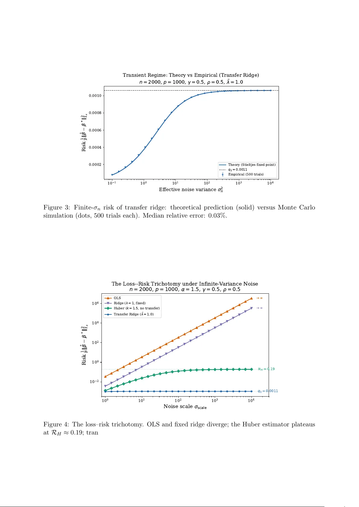
The Conjugate Domain Dichotomy: Exact Risk of M-Estimators under Infinite-Variance Noise in High Dimensions

The Conjugate Domain Dic hotom y: Exact Risk of M-Estimators under Infinite-V ariance Noise in High Dimensions Charalamp os Agirop oulos Departmen t of Economics, Univ ersity of Piraeus hagyropoylos@unipi.gr Marc h 31, 2026 Abstract This pap er studies high-dimensional M-estimation in the prop ortional asymptotic regime ( p/n → γ > 0) when the noise distribution has infinite v ariance. F or noise with regularly- v arying tails of index α ∈ (1 , 2), w e establish that the asymptotic behavior of a regularized M-estimator is gov erned b y a single geometric prop ert y of the loss function: the b oundedness of the domain of its F enc hel conjugate. When this conjugate domain is bounded — as is the case for the Hub er, absolute-v alue, and quan tile loss functions — the dual v ariable in the min-max formulation of the estimator is confined, the effectiv e noise reduces to the finite first absolute moment of the noise distribution, and the estimator achiev es b ounded risk without recourse to external information. When the conjugate domain is unbounded — as for the squared loss — the dual v ariable scales with the noise, the effective noise inv olves the diverging second moment, and b ounded risk can b e ac hieved only through transfer regularization tow ard an external prior. F or the squared-loss class sp ecifically , we derive the exact asymptotic risk via the Conv ex Gaussian Minimax Theorem under a noise-adapted regularization scaling λ n = ˜ λ σ 2 n . The resulting risk conv erges to a universal flo or q Σ = p − 1 ∥ β ∗ − β 0 ∥ 2 Σ x that is indep endent of the regularizer, yielding a loss–risk trichotom y: squared-loss estimators without transfer div erge; Hub er-loss estimators ac hieve bounded but non-v anishing risk; transfer-regularized estimators attain q Σ . Keywor ds: Conjugate domain, Conv ex Gaussian minimax theorem, heavy-tailed noise, high- dimensional regression, M-estimation, phase transition, prop ortional asymptotics, regular v ariation, transfer learning, Winsorization. MSC2020: 62J07, 62F35, 60B20, 62C20. Con ten ts 1 In tro duction 2 1.1 Bac kground and motiv ation . . . . . . . . . . . . . . . . . . . . . . . . . . . . . . 2 1.2 A structural tension . . . . . . . . . . . . . . . . . . . . . . . . . . . . . . . . . . 3 1.3 The conjugate domain as the go verning mechanism . . . . . . . . . . . . . . . . . 3 1.4 Summary of contributions . . . . . . . . . . . . . . . . . . . . . . . . . . . . . . . 4 1.5 Scop e and limitations . . . . . . . . . . . . . . . . . . . . . . . . . . . . . . . . . 4 1.6 Related work . . . . . . . . . . . . . . . . . . . . . . . . . . . . . . . . . . . . . . 4 2 The Conjugate Domain Dichotom y 5 2.1 Assumptions and definitions . . . . . . . . . . . . . . . . . . . . . . . . . . . . . . 5 2.2 Statemen t of the dichotom y . . . . . . . . . . . . . . . . . . . . . . . . . . . . . . 6 1 3 Exact risk c haracterization 7 3.1 The truncation bridge . . . . . . . . . . . . . . . . . . . . . . . . . . . . . . . . . 7 3.2 F ailure of squared-loss estimation . . . . . . . . . . . . . . . . . . . . . . . . . . . 7 3.3 Noise-adapted regularization and exact risk . . . . . . . . . . . . . . . . . . . . . 8 3.4 The universal risk flo or . . . . . . . . . . . . . . . . . . . . . . . . . . . . . . . . . 9 3.5 The loss–risk trichotom y . . . . . . . . . . . . . . . . . . . . . . . . . . . . . . . . 9 3.6 Design universalit y . . . . . . . . . . . . . . . . . . . . . . . . . . . . . . . . . . . 10 4 Pro ofs 10 4.1 Pro of arc hitecture for the Conjugate Domain Dic hotomy . . . . . . . . . . . . . . 10 4.2 Pro of of the exact risk formula . . . . . . . . . . . . . . . . . . . . . . . . . . . . 11 5 Numerical exp erimen ts 11 6 Discussion 12 6.1 The tw o-p enalt y decomposition . . . . . . . . . . . . . . . . . . . . . . . . . . . . 12 6.2 Op en problems . . . . . . . . . . . . . . . . . . . . . . . . . . . . . . . . . . . . . 12 A T run cation univ ersality: full details 14 B CGMT reduction and compactification 14 C A O conv ergence and the univ ersal flo or 14 D Conjugate Domain Dic hotomy: pro of details 15 E Design univ ersality: condition verification 15 1 In tro duction 1.1 Bac kground and motiv ation Consider the linear mo del y = X β ∗ + w , (1) where X ∈ R n × p is a design matrix with indep endent rows drawn from N (0 , Σ x ), β ∗ ∈ R p is the unkno wn regression parameter, and w ∈ R n is a noise vector with indep endent and identically distributed entries. In the prop ortional asymptotic regime p/n → γ ∈ (0 , ∞ ), a substantial b o dy of recent work has established precise characterizations of the estimation risk for regularized least-squares estimators under finite noise v ariance. The foundational results of Dobriban and W ager [ 2018 ] and Hastie et al. [ 2022 ] for ridge regression, the extension to general conv ex regularizers via the Conv ex Gaussian Minimax Theorem (CGMT) by Thramp oulidis et al. [ 2015 , 2018 ], and the analysis of b enign o v erfitting b y Bartlett et al. [ 2020 ], Tsigler and Bartlett [ 2023 ] all rely on the assumption that the noise v ariance is finite and fixed as n → ∞ . The present work considers the question of what can b e said when this assumption fails. Distributions with regularly-v arying tails — including P areto distributions, Student- t distri- butions with few degrees of freedom, and α -stable laws with stabilit y index α < 2 — arise naturally in the mo deling of financial returns, insurance claims, netw ork traffic, and seismological recordings Resnick [ 2007 ], Samoro dnitsky and T aqqu [ 1994 ]. F or such distributions with tail index α ∈ (1 , 2), the first momen t is finite but the v ariance is infinite. The classical bias–v ariance decomp osition, which underpins muc h of the theory of high-dimensional regression, is no longer applicable in this setting. 2 1.2 A structural tension A standard approach to handling infinite-v ariance noise is Winsorization : clipping the noise at a sample-size-dep enden t threshold τ n = n 1 /α to pro duce a proxy mo del with finite but growing v ariance. W e show (Theorem 3.1 ) that this pro cedure yields an effective v ariance σ 2 n = 2 c 2 − α n (2 − α ) /α (1 + o (1)) (2) for any noise distribution satisfying P ( | w | > t ) ∼ c t − α as t → ∞ , where the asymptotic constant c > 0 and the rate dep end only on the tail parameters α and c . This div erging effective v ariance gives rise to a noteworth y tension. The total Fisher information contained in the observ ations satisfies I n = n/σ 2 n = Θ( n (2 α − 2) /α ) → ∞ for all α > 1 (Theorem 3.2 ), so the data are, in an information-theoretic sense, increasingly informativ e ab out β ∗ . It is therefore not the case that the observ ations lack the information necessary for consistent estimation. A t the same time, an y estimator constructed b y minimizing a squared-loss ob jectiv e 1 2 n ∥ y − X β ∥ 2 inherits the div erging noise v ariance directly . The risk of the ordinary least-squares estimator gro ws as Θ( σ 2 n ). Ridge regression with a fixed regularization parameter exhibits the same divergen t b ehavior. Even when the regularization strength is adapted to the noise level — sp ecifically , when λ n = Θ( σ 2 n ) — the estimator merely exchanges div erging v ariance for an irreducible bias that dep ends on the distance b etw een the truth and the regularization center (Theorem 3.3 ). The difficulty , then, is not a lack of information in the data, but rather a mismatc h b et ween the loss function and the noise structure. The squared loss, through its sensitivit y to the second momen t of the noise, amplifies the diverging v ariance into the estimation risk. 1.3 The conjugate domain as the go verning mechanism The central contribution of this pap er is the iden tification of the precise geom etric prop erty of the loss function that determines whether an M-estimator can tolerate infinite-v ariance noise. This prop ert y is the b ounde dness of the domain of the F enchel c onjugate . Recall that any prop er closed conv ex loss function L admits the dual represen tation L ( a ) = sup u ∈ dom( L ∗ ) { ua − L ∗ ( u ) } , where L ∗ ( u ) = sup t { ut − L ( t ) } is the F enchel conjugate. In the min-max formulation of the M-estimator that arises within the CGMT framework, the dual v ariable u i asso ciated with the i -th observ ation is constrained to dom ( L ∗ ). The interaction b et ween this constrain t and the noise w i is the mec hanism through which the loss function either amplifies or attenuates the effect of hea vy tails: • When dom ( L ∗ ) ⊆ [ − K, K ] for some K > 0, eac h dual v ariable satisfies | u i | ≤ K . The noise coupling term n − 1 P n i =1 u i w i is then b ounded b y K · n − 1 P | w i | , which in volv es only the first absolute moment of the noise. Since E [ | w | ] < ∞ whenev er α > 1, this quantit y remains b ounded, and the estimator achiev es finite risk. • When dom ( L ∗ ) = R , the optimal dual v ariable scales with the noise (for the squared loss, u ∗ i ∝ w i ), and the noise coupling inv olves the second moment n − 1 P w 2 i , whic h div erges when α < 2. The squared loss, with L ∗ ( u ) = u 2 / 2 and dom ( L ∗ ) = R , is the prototypical loss with un b ounded conjugate domain. The Hub er loss, with L ∗ ( u ) = u 2 / 2 for | u | ≤ k and L ∗ ( u ) = + ∞ for | u | > k , is the prototypical loss with b ounded conjugate domain. More generally , a loss function has b ounded conjugate domain if and only if it grows at least linearly at infinity: lim inf | t |→∞ L ( t ) / | t | > 0. This characterization encompasses the absolute-v alue loss, the quantile loss, the log-cosh loss, and all Hub er-t yp e losses. W e formalize this classification as the Conjugate Domain Dichotomy (Theorem 2.5 ). 3 1.4 Summary of contributions The pap er makes the following contributions. (i) The Conjugate Domain Dichotomy (Theorem 2.5 ). W e prov e that, under regularly-v arying noise with index α ∈ (1 , 2), a regularized M-estimator achiev es b ounded risk if and only if its loss function has b ounded conjugate domain. The pro of iden tifies the first-versus-second momen t mec hanism described ab o ve as the quan titative explanation (Corollary 2.6 ). (ii) The moment hier ar chy (Remark 2.7 ). W e extend the dichotom y to a contin uous classification: a loss whose conjugate grows as | u | q requires finiteness of the q -th noise moment. This yields a complete corresp ondence b etw een conjugate growth rate and noise momen t requiremen ts. (iii) T runc ation universality (Theorem 3.1 ). F or an y noise distribution in the domain of attraction of an α -stable law, Winsorization at the threshold τ n = n 1 /α pro duces the effective v ariance ( 2 ) , with concentrat ion of the empirical squared norm around this deterministic equiv alent. (iv) Exact risk char acterization via the CGMT (Theorem 3.5 ). F or squared-loss estimators with noise-adapted regularization λ n = ˜ λ σ 2 n , w e deriv e the exact asymptotic risk as the solution of a fixed-p oint system inv olving the proximal op erator of the regularizer and the sp ectral distribution of Σ x . (v) Universal risk flo or (Theorem 3.6 ). In the diverging-noise limit, the fixed-p oint system admits an explicit solution: the risk con v erges to q Σ = p − 1 ∥ β ∗ − β 0 ∥ 2 Σ x , indep enden t of the choice of co erciv e conv ex regularizer. This universalit y arises from the proximal op erator collapsing under a diverging step size. (vi) The loss–risk trichotomy (Theorem 3.7 ). Combining the dichotom y with the exact risk c haracterization yields three distinct regimes: squared-loss estimators without transfer ha ve div erging risk; Hub er-loss estimators ac hiev e b ounded risk R H < ∞ but cannot eliminate the prop ortional-regime p enalty; transfer-regularized squared-loss estimators attain q Σ ≪ R H when the prior is informative. (vii) Design universality (Theorem 3.9 ). All results extend from Gaussian to sub-Gaussian designs b y verification of the conditions in the univ ersalit y framework of Montanari and Saeed [ 2022 ]. 1.5 Scop e and limitations The results apply to prop er closed conv ex loss functions paired with co ercive conv ex regularizers. The analysis do es not cov er non-conv ex p enalties such as SCAD or MCP , nor do es it address the case of heavy-tailed cov ariates, which would require tools b ey ond the CGMT. The tail index is restricted to α ∈ (1 , 2); for α ≤ 1 the mean is infinite and the truncation bridge of Theorem 3.1 do es not apply . W e do not address exact support recov ery , which requires techniques distinct from the L 2 -risk analysis pursued here, nor data-driv en selection of the regularization parameter. 1.6 Related w ork Pr op ortional-r e gime risk char acterization. The precise risk of ridge regression in the prop ortional regime was established by Dobriban and W ager [ 2018 ] and Hastie et al. [ 2022 ], building on the Marchenk o–P astur la w Marc henk o and Pastur [ 1967 ] and companion Stieltjes transform tec hniques Bai and Silverstein [ 2010 ]. The CGMT, developed b y Thramp oulidis et al. [ 2015 , 2018 ] from Gordon’s Gaussian comparison inequality Gordon [ 1988 ], extended these results to general conv ex regularizers and M-estimators. The phenomena of b enign o verfitting Bartlett et al. [ 2020 ], Tsigler and Bartlett [ 2023 ] and double descent Belkin et al. [ 2019 ], Adv ani and 4 Saxe [ 2020 ], Mei and Montanari [ 2022 ] ha ve b een analyzed within this framework. All of these w orks assume finite and fixed noise v ariance. He avy-taile d r e gr ession. Estimation under heavy-tailed noise has b een studied from sev eral p ersp ectiv es. Lugosi and Mendelson [ 2019 ] established sub-Gaussian estimation rates via median- of-means techniques, and Adomait yt ˙ e et al. [ 2024 ] derived exact asymptotics under heavy-tailed data in a related high-dimensional setting. The robust statistics literature, originating with Hub er [ 1964 ] and developed in Hub er and Ronchetti [ 2009 ], provides the classical foundation for M-estimation with b ounded influence functions. High-dimensional robust regression was analyzed b y El Karoui et al. [ 2013 ] for fixed noise v ariance. T r ansfer le arning. T ransfer learning in high-dimensional linear mo dels was studied by Dar and Baraniuk [ 2022 ], who c haracterized the double descen t phenomenon under task transfer, and b y Li et al. [ 2022 ], who established minimax rates for transfer estimation. Universality. Design universalit y for empirical risk minimization was established by Montanari and Saeed [ 2022 ] via a con tinuous in terp olation argumen t, and b y Hu and Lu [ 2023 ] for random feature mo dels. The present work differs from the ab ov e in tw o principal resp ects. First, w e consider a regime in which the noise v ariance diverges with the sample size — a qualitativ ely different setting from the fixed-v ariance regime studied in the CGMT and proportional-asymptotics literatures. Second, we identify the conjugate domain of the loss function as the geometric prop ert y that go verns whether an estimator can tolerate this divergence, providing a classification that applies to all conv ex losses simultaneously rather than analyzing sp ecific estimators individually . 2 The Conjugate Domain Dic hotomy 2.1 Assumptions and definitions W e w ork throughout with the observ ation mo del ( 1 ) under the follo wing conditions. Assumption 2.1 (Design and dimensionality) . The design matrix satisfies X = Z Σ 1 / 2 x , where Z ∈ R n × p has indep enden t standard Gaussian entries, and Σ x ∈ R p × p is p ositiv e definite with empirical sp ectral distribution con verging w eakly to a compactly supp orted probabilit y measure µ on (0 , ∞ ). The dimensions satisfy p/n → γ ∈ (0 , ∞ ) as n, p → ∞ . Assumption 2.2 (Regularly-v arying noise) . The noise v ariables w 1 , w 2 , . . . are indep enden t and identically distributed with E [ w i ] = 0 and tail b ehavior P ( | w i | > t ) = c t − α (1 + o (1)) as t → ∞ , for some α ∈ (1 , 2) and c > 0. Assumption 2.2 places the noise distribution in the domain of attraction of an α -stable law. The condition α > 1 ensures that E [ | w i | ] < ∞ , while α < 2 implies E [ w 2 i ] = ∞ . The requiremen t that the slowly v arying comp onent of the tail conv erges to a constant (rather than b eing an arbitrary slowly v arying function) is imp osed for clarit y; it is satisfied by Student- t , Pareto, and α -stable distributions. Definition 2.3 (Winsorization) . F or a threshold τ > 0, the Winsorized noise is w ( τ ) i = w i 1 {| w i |≤ τ } + τ sign ( w i ) 1 {| w i | >τ } . W e set τ n = n 1 /α and write σ 2 n = E [( w ( τ n ) i ) 2 ] for the effectiv e v ariance. Definition 2.4 (Conjugate domain classes) . Let L : R → R ∪ { + ∞} b e a prop er closed con vex function with F enchel conjugate L ∗ ( u ) = sup t { ut − L ( t ) } . W e sa y that L has b ounde d c onjugate domain if there exists K > 0 such that dom ( L ∗ ) = { u : L ∗ ( u ) < ∞} ⊆ [ − K, K ], and unb ounde d c onjugate domain if dom( L ∗ ) = R . A standard result in conv ex analysis relates the conjugate domain to the growth rate of the loss: dom ( L ∗ ) is b ounded if and only if lim inf | t |→∞ L ( t ) / | t | > 0. Thus the class of losses 5 with b ounded conjugate domain consists precisely of those that grow at least linearly at infinit y . Among common loss functions, the squared loss L ( t ) = t 2 / 2 is the unique standard example with un b ounded conjugate domain. The Hub er loss ρ k ( t ) = ( t 2 / 2 | t | ≤ k , k | t | − k 2 / 2 | t | > k , the absolute-v alue loss L ( t ) = | t | , the log-cosh loss L ( t ) = log cosh ( t ), and the quantile loss L ( t ) = t ( τ − 1 { t< 0 } ) all hav e b ounded conjugate domain. 2.2 Statemen t of the dic hotomy W e consider the general regularized M-estimator ˆ β L = arg min β ∈ R p 1 n n X i =1 L ( y i − x ⊤ i β ) + λ n R ( β ) , (3) where R : R p → R ∪ { + ∞} is a prop er closed co ercive conv ex regularizer (meaning R ( β ) → ∞ as ∥ β ∥ → ∞ ) and λ n > 0 is the regularization parameter. Theorem 2.5 (Conjugate Domain Dic hotomy) . Under Assumptions 2.1 – 2.2 , the fol lowing hold for the estimator ( 3 ) : (B) If L has b ounde d c onjugate domain ( dom ( L ∗ ) ⊆ [ − K, K ] ), then for any fixe d λ > 0 and any c o er cive c onvex R , 1 p ∥ ˆ β L − β ∗ ∥ 2 Σ x P − → R L ( K, λ, γ , µ ) < ∞ , wher e R L do es not dep end on σ 2 n . (U) If L has unb ounde d c onjugate domain ( dom( L ∗ ) = R ), then: (U1) Without tr ansfer r e gularization ( R ( β ) c enter e d at the origin), the risk either diver ges (if λ n = o ( σ 2 n ) ) or c onver ges to p − 1 ∥ β ∗ ∥ 2 Σ x (if λ n = Θ( σ 2 n ) ). (U2) With tr ansfer r e gularization R ( β − β 0 ) and λ n = ˜ λ σ 2 n for fixe d ˜ λ > 0 , the risk c onver ges to q Σ = p − 1 ∥ β ∗ − β 0 ∥ 2 Σ x . The pro of is giv en in Section 4.1 and Appendix D. The following corollary makes the mec hanism explicit. Corollary 2.6 (The moment mechanism) . Part (B) of The or em 2.5 holds b e c ause the c onstr aint u i ∈ [ − K, K ] ensur es that the noise c oupling in the CGMT dual satisfies | n − 1 P u i w ( τ n ) i | ≤ K · n − 1 P | w ( τ n ) i | P − → K E [ | w | ] < ∞ . Part (U) holds b e c ause the unc onstr aine d dual u ∗ i ∝ w i yields a c oupling that involves n − 1 P w 2 i ≍ σ 2 n → ∞ . R emark 2.7 (The momen t hierarc hy) . The dichotom y generalizes to a con tinuous classification. If the conjugate satisfies L ∗ ( u ) ∼ c q | u | q as | u | → ∞ for some q ≥ 1, then the optimal dual v ariable has magnitude | u ∗ i | = O ( | w i | 1 / ( q − 1) ) (b y the first-order condition of the dual), and the noise coupling inv olv es the q / ( q − 1)-th moment of w . The estimator therefore ac hieves b ounded risk if and only if α ≥ q / ( q − 1), or equiv alently q ≥ α/ ( α − 1). F or q = 1 (b ounded domain, e.g., Hub er), the requirement is α > 1 (finite mean). F or q = 2 (quadratic conjugate, i.e., squared loss), the requirement is α ≥ 2 (finite v ariance). 6 3 Exact risk c haracterization This section develops the quantitativ e predictions that underlie the dichotom y . W e b egin with the truncation bridge that connects regularly-v arying noise to a div erging-v ariance pro xy mo del, then present the exact risk formulas for the squared-loss class, and conclude with the trichotom y that combin es b oth classes. 3.1 The truncation bridge Theorem 3.1 (T runcation universalit y) . Under Assumption 2.2 , with τ n = n 1 /α and σ 2 n = E [( w ( τ n ) ) 2 ] : (i) σ 2 n = 2 c 2 − α n (2 − α ) /α (1 + o (1)) . (ii) n − 1 ∥ w ( τ n ) ∥ 2 /σ 2 n P − → 1 . Pr o of of (i) . By definition of the Winsorized v ariable, E [( w ( τ ) ) 2 ] = E [ w 2 1 {| w |≤ τ } ] + τ 2 P ( | w | > τ ). Applying in tegration b y parts to the first term with the lay er-cake represen tation yields E [ w 2 1 {| w |≤ τ } ] = R τ 0 2 t ¯ F ( t ) dt − τ 2 ¯ F ( τ ), where ¯ F ( t ) = P ( | w | > t ). Adding the Winsorization b oundary term τ 2 ¯ F ( τ ) pro duces a cancellation: E [( w ( τ ) ) 2 ] = Z τ 0 2 t ¯ F ( t ) dt. (4) This cancellation is sp ecific to Winsorization; simple truncation ( w 1 {| w |≤ τ } ) retains the b oundary term. The in tegrand 2 t ¯ F ( t ) = 2 c t 1 − α (1 + o (1)) is regularly v arying with index 1 − α > − 1, so Karamata’s theorem [ Bingham et al. , 1987 , Theorem 1.5.11] giv es R τ 0 2 t ¯ F ( t ) dt ∼ 2 c 2 − α τ 2 − α . Setting τ = n 1 /α yields the result. The mean correction is handled b y the dominated con v ergence theorem: since | w ( τ n ) | ≤ | w | and E [ | w | ] < ∞ (as α > 1), we hav e | E [ w ( τ n ) ] | ≤ E [ | w | 1 {| w | >τ n } ] → 0, so ( E [ w ( τ n ) ]) 2 = o (1) is negligible compared to the diverging second momen t. Pr o of of (ii) . The concentration of n − 1 P ( w ( τ n ) i ) 2 around σ 2 n requires care, b ecause the stan- dard fourth-momen t metho d is exactly b orderline. Indeed, the same in tegration-by-parts and Karamata argumen t gives E [( w ( τ n ) ) 4 ] ∼ 4 c 4 − α n (4 − α ) /α , and the relative v ariance n − 1 E [( w ( τ n ) ) 4 ] ( σ 2 n ) 2 ≍ n − 1+(4 − α ) /α − 2(2 − α ) /α = n 0 = O (1) , whic h do es not tend to zero. This b orderline b ehavior is not a pro of artifact: the ratio τ 2 n /σ 2 n ≍ n gro ws linearly , placing the problem at the exact threshold where CL T-type normalization pro duces non-degenerate fluctuations. W e circum ven t this obstruction via a truncation-based double-limit argument on the tr iangular arra y { ( w ( τ n ) i ) 2 /σ 2 n } 1 ≤ i ≤ n . Define Y n,i = ( w ( τ n ) i ) 2 /σ 2 n − 1 and S n = n − 1 P Y n,i . F or any M > 0, decomp ose S n = A n ( M ) + B n ( M ), where A n ( M ) = n − 1 P Y n,i 1 {| Y n,i |≤ M } . The b ounded part satisfies V ar ( A n ( M )) ≤ M 2 /n → 0 by Cheb yshev’s inequalit y . The tail part satisfies P ( | B n ( M ) | > δ ) ≤ δ − 1 E [ | Y n, 1 | 1 {| Y n, 1 | >M } ] b y Mark ov’s inequality , and the Karamata structure of the tail ensures that lim sup n E [ | Y n, 1 | 1 {| Y n, 1 | >M } ] → 0 as M → ∞ . Cho osing M large and then n large completes the argumen t. F ull details are in App endix A. 3.2 F ailure of squared-loss estimation Theorem 3.2 (Fisher information diverges) . Under Assumption 2.2 , I n = n/σ 2 n = Θ( n (2 α − 2) /α ) → ∞ . 7 Pr o of. The p er-observ ation Fisher information for a lo cation family with v ariance σ 2 n satisfies I 1 = O (1 /σ 2 n ). With n indep enden t observ ations, I n = n · I 1 = Θ( n/σ 2 n ). Since (2 α − 2) /α > 0 for α > 1, the result follo ws. Theorem 3.3 (Divergence of L 2 -estimation without transfer) . Under Assumptions 2.1 – 2.2 with p/n → γ > 0 and σ 2 n → ∞ : (i) The OLS estimator (when γ < 1 ) has risk Θ( σ 2 n ) → ∞ . (ii) R idge r e gr ession with fixe d λ > 0 has risk Θ( σ 2 n ) → ∞ . (iii) Any r e gularize d estimator with λ n = o ( σ 2 n ) has diver ging risk. (iv) With noise-adapte d r e gularization λ n = ˜ λσ 2 n c enter e d at the origin, the risk c onver ges to p − 1 ∥ β ∗ ∥ 2 Σ x . Pr o of. P arts (i)–(ii) follo w from the standard bias–v ariance decomp osition in the prop ortional regime, where the v ariance comp onen t is prop ortional to σ 2 n . P art (iii) follows from the failure of the compactification argumen t (Lemma 4.1 ) when ˜ λ = λ n /σ 2 n → 0: the regularizer cannot confine the estimator. P art (iv) is a sp ecial case of Theorem 3.6 with β 0 = 0. Theorems 3.2 and 3.3 together rev eal that the failure of squared-loss estimation under div erging noise is not an information-theoretic limitation but a structural vulnerability of the loss function. The data contain sufficient information for consistent estimation; the squared loss simply cannot extract it. This observ ation is cen tral to the motiv ation for the Conjugate Domain Dich otom y . 3.3 Noise-adapted regularization and exact risk T o obtain meaningful risk b ounds for the squared-loss class, the regularization strength must scale with the noise p ow er. Definition 3.4 (Noise-adapted regularization) . The effe ctive r e gularization str ength is ˜ λ = λ n /σ 2 n , treated as an O (1) constant. This scaling ensures that the regularization grows in step with the noise, pro ducing a well- defined trade-off b etw een bias and v ariance in the limit. When α = 2 (finite v ariance), σ 2 n = Θ(1) and the standard fixed- λ regime is reco vered. Theorem 3.5 (Exact risk at finite noise lev el) . Under Assumptions 2.1 – 2.2 , for the tr ansfer- r e gularize d estimator ˆ β = arg min β ∈ R p 1 2 n ∥ y − X β ∥ 2 + ˜ λ σ 2 n R ( β − β 0 ) with c o er cive c onvex R and p/n → γ , the risk p − 1 ∥ ˆ β − β ∗ ∥ 2 Σ x c onver ges in pr ob ability to a deterministic limit R char acterize d by the fixe d-p oint e quation τ 2 = 1 + γ R ( τ ) , wher e R ( τ ) = E S,ζ " S  pro x ˜ λσ 2 n S − 1 r  ∆ S − σ n τ √ S ζ  − ∆ S  2 # , (5) with S ∼ µ (the limiting sp e ctr al distribution of Σ x ), ζ ∼ N (0 , 1) indep endent, and ∆ S denoting the pr oje ction of ∆ = β ∗ − β 0 onto the eigensp ac e c orr esp onding to eigenvalue S . F or ridge r e gularization ( R = 1 2 ∥ · ∥ 2 ), the risk admits the close d-form Stieltjes r epr esentation R ridge = µ 2 E S  S ∆ 2 S ( S v + µ ) 2  + σ 2 n n v E S  S 2 ( S v + µ ) 2  , (6) wher e µ = ˜ λσ 2 n and v is the unique p ositive solution of v − 1 = 1 + γ E S [ S ( S v + µ ) − 1 ] . The pro of pro ceeds through the CGMT framew ork and is given in Section 4.2 and App endix B– C. 8 3.4 The univ ersal risk flo or Theorem 3.6 (Universal risk flo or) . Under Assumptions 2.1 – 2.2 , for any c o er cive c onvex R with arg min R = { 0 } and any ˜ λ > 0 : 1 p ∥ ˆ β − β ∗ ∥ 2 Σ x P − → q Σ = 1 p ∥ β ∗ − β 0 ∥ 2 Σ x . This limit is indep endent of the r e gularizer R , the effe ctive str ength ˜ λ , and the noise distribution b eyond the tail index α . Pr o of. In the CGMT auxiliary optimization, the pro ximal step size for co ordinate j in the eigen basis of Σ x is η j = ˜ λσ 2 n /s j , where s j is the j -th eigenv alue of Σ x . Since σ 2 n → ∞ and s j is b ounded a w ay from zero (b y the compact supp ort of µ ), w e ha ve η j → ∞ for every j . The asymptotic b eha vior of the proximal op erator under diverging step size is well known: for any prop er closed conv ex function r with arg min r = { 0 } , pro x η r ( x ) → 0 as η → ∞ for an y x [ Bausc hke and Com b ettes , 2017 , Proposition 12.29]. In our setting, the argumen t of the pro ximal op erator is ∆ s j − σ n τ ζ j / √ s j = O ( σ n ), while the step size is O ( σ 2 n ). Therefore the pro ximal output is O ( σ n /σ 2 n ) = O (1 /σ n ) → 0. Setting ϕ j = v j + ∆ s j (the estimator’s deviation from the prior in co ordinate j ), w e obtain ϕ ∗ j → 0, i.e., v ∗ j → − ∆ s j . The risk b ecomes 1 p X j s j ( v ∗ j ) 2 → 1 p X j s j ∆ 2 s j = 1 p ∥ ∆ ∥ 2 Σ x = q Σ . The univ ersality of the risk floor across regularizers has a clear in terpretation: under div erging noise, the proximal op erator with diverging step size maps all inputs to the minimizer of r , erasing any dep endence on the regularizer’s geometry . Ridge, Lasso, elastic net, and group Lasso all pro duce the same limiting risk. The regularizer matters only in the transient regime at finite noise levels, where it gov erns the rate of conv ergence to q Σ . 3.5 The loss–risk trichotom y Com bining the b ounded-domain result (Theorem 2.5 (B)) with the exact squared-loss c haracteri- zation (Theorems 3.5 – 3.6 ) and the Hub er analysis yields the following trichotom y . Theorem 3.7 (Loss–risk trichotom y) . Under Assumptions 2.1 – 2.2 : (a) Squared loss without transfer. The risk either diver ges or c onver ges to p − 1 ∥ β ∗ ∥ 2 Σ x > 0 . (b) Hub er loss without transfer. The risk c onver ges to R H ( k , λ, γ , µ ) < ∞ , which do es not dep end on σ 2 n but satisfies R H > 0 in the pr op ortional r e gime. (c) Squared loss with transfer. The risk c onver ges to q Σ = p − 1 ∥ β ∗ − β 0 ∥ 2 Σ x . When the prior is informative, q Σ ≪ R H . The trichotom y reveals that tw o distinct p enalties imp ede estimation under infinite-v ariance noise. The he avy-tail p enalty arises from the in teraction b etw een the loss function’s conjugate geometry and the noise momen t structure; it is eliminated b y any loss with b ounded conjugate domain. The high-dimensional p enalty R H > 0 arises from the prop ortional regime p/n → γ > 0; it p ersists ev en when the effective noise is b ounded and is b ypassed only when external structural information (the transfer prior) is a v ailable. R emark 3.8 (When the Hub er estimator dominates) . If the transfer prior is p o or ( q Σ > R H ), the Hub er estimator strictly dominates the transfer-regularized squared-loss estimator. The practitioner therefore faces a genuine trade-off: accurate prior information yields low er risk via transfer, but absent such information, a robust loss function provides a safer alternative. 9 3.6 Design univ ersalit y Theorem 3.9 (Design univ ersality) . Al l r esults of The or ems 2.5 – 3.7 hold when Assumption 2.1 is r elaxe d to al low Z ij to b e indep endent and identic al ly distribute d sub-Gaussian r andom variables with E [ Z ij ] = 0 , E [ Z 2 ij ] = 1 , and ∥ Z ij ∥ ψ 2 ≤ K . Pr o of. The result follows from the univ ersality framework of Mon tanari and Saeed [ 2022 ]. The fiv e conditions of their Corollary 3 are verified in App endix E: (i) the squared loss has lo cally Lipsc hitz gradien t; (ii) the feasible set is compact by Lemma 4.1 ; (iii) the regularizer is lo cally Lipsc hitz on b ounded sets; (iv) the design x i = Σ 1 / 2 x ¯ x i with sub-Gaussian ¯ x i satisfies the point wise normalit y condition; (v) the Winsorized noise is b ounded (hence sub-Gaussian) and indep endent of the design. The key observ ation is that the univ ersality mechanism acts on the design matrix, while the noise passes through unc hanged regardless of its magnitude or distribution. 4 Pro ofs 4.1 Pro of arc hitecture for the Conjugate Domain Dichotom y The pro of of Theorem 2.5 pro ceeds through the CGMT in three stages. Stage I: Comp actific ation. The following lemma ensures that the optimizer remains b ounded. Lemma 4.1 (Compactification) . Under noise-adapte d r e gularization λ n = ˜ λσ 2 n with c o er cive c onvex R , ther e exists a deterministic c onstant C > 0 , indep endent of n , such that P ( ∥ ˆ β − β ∗ ∥ Σ x > C ) → 0 . Pr o of. The ob jectiv e at v = 0 equals (2 nσ 2 n ) − 1 ∥ w ( τ n ) ∥ 2 + ˜ λR (∆), whic h con verges in probability to 1 2 + ˜ λR (∆) by Theorem 3.1 (ii). On the sphere ∥ v ∥ Σ x = C , the co ercivity of R ensures ˜ λR ( v + ∆) > 1 2 + ˜ λR (∆) for C sufficien tly large. Since the minimizer ac hiev es a v alue at most the baseline, it must lie inside the ball. An imp ortant structural observ ation emerges from the pro of: the quadratic confinemen t pro vided b y the design matrix, (2 nσ 2 n ) − 1 ∥ X v ∥ 2 → ∥ v ∥ 2 Σ x / (2 σ 2 n ) → 0, v anishes under the σ 2 n normalization. The regularizer is therefore the sole mechanism confining the estimator under div erging noise. Stage II: CGMT r e duction. With the feasible set compact, the CGMT Thramp oulidis et al. [ 2015 ] replaces the bilinear form u ⊤ Z (Σ 1 / 2 x v ) in the Primary Optimization with indep endent Gaussian v ectors g ∼ N (0 , I n ) and h ∼ N (0 , Σ x ), pro ducing the Auxiliary Optimization. The noise vector w ( τ n ) en ters b oth formu lations identically as an additiv e term; it is not affected by Gordon’s comparison inequality , which op erates exclusively on the Gaussian bilinear form. Stage III: Sc alarization and the moment me chanism. In the A O, optimizing ov er the dual v ariable u yields co ordinate-wise up dates. F or b ounded dom ( L ∗ ): each u i is constrained to [ − K, K ], so u ∗ i = clip ( w ( τ n ) i + ∥ ˜ v ∥ g i , − K , K ). The effectiv e noise n − 1 ∥ u ∗ ∥ 2 ≤ K 2 is b ounded deterministically . Mean while, n − 1 P | w ( τ n ) i | P − → E [ | w | ] < ∞ b y the law of large num b ers and the dominated conv ergence theorem (since | w ( τ n ) | ≤ | w | and E [ | w | ] < ∞ for α > 1). The AO scalarization pro duces a fixed-p oin t system with all terms O (1), yielding finite risk. F or un b ounded dom ( L ∗ ) (e.g., L ∗ ( u ) = u 2 / 2): u ∗ i = w ( τ n ) i + ∥ ˜ v ∥ g i is unconstrained, so n − 1 ∥ u ∗ ∥ 2 ≍ σ 2 n → ∞ . After σ 2 n normalization, the AO reduces to the fixed-p oint system of Theorem 3.5 , with the univ ersal flo or following from the proximal collapse of Theorem 3.6 . F ull details are in App endices B–D. 10 1 0 0 1 0 1 1 0 2 1 0 3 N o i s e s c a l e s c a l e 1 0 3 1 0 2 1 0 1 1 0 0 1 0 1 1 0 2 1 0 3 1 0 4 Risk (log scale) T h e S t r u c t u r a l P a r a d o x : L 2 D i v e r g e n c e v s T r a n s f e r C o n v e r g e n c e OLS R i d g e ( = 1 , f i x e d ) T r a n s f e r R i d g e ( = 1 . 0 ) q = 0 . 0 0 1 1 Figure 1: Risk as a function of noise scale for three squared-loss estimators. OLS and fixed- λ ridge exhibit p ow er-la w div ergence; transfer ridge is constant at q Σ ≈ 0 . 001. 4.2 Pro of of the exact risk formula The deriv ation of Theorem 3.5 follo ws the CGMT scalarization after Stages I–I I ab ov e. The Primary Optimization, after normalization by σ 2 n , takes the form min v ∈S C max u ∈ R n u ⊤ w ( τ n ) nσ n − u ⊤ Z Σ 1 / 2 x v nσ n − ∥ u ∥ 2 2 n + ˜ λ R ( v + ∆) . Gordon’s comparison replaces the bilinear term, and the empirical quantities concentrate by Theorem 3.1 and standard Gaussian concen tration. After optimizing ov er u in closed form and passing to the deterministic limit (using uniform conv ergence on the compact set S C ), the risk is c haracterized b y the fixed-p oint system ( 5 ) . F or ridge regression, the proximal op erator reduces to the linear map x 7→ x/ (1 + η ), yielding the companion Stieltjes representation ( 6 ) . F ull details app ear in App endix C. 5 Numerical exp eriments W e present Monte Carlo simulations that verify the theoretical predictions. All exp erimen ts use n = 2000 observ ations, p = 1000 cov ariates ( γ = 0 . 5), an AR(1) cov ariance structure (Σ x ) ij = 0 . 5 | i − j | , and Student- t noise with 1 . 5 degrees of freedom ( α = 1 . 5). The signal β ∗ has 10% non-zero en tries; the transfer prior β 0 = β ∗ + ∆ has misalignment ∥ ∆ ∥ = 1. Eac h p oint represen ts the a v erage of 500 indep endent replications. Figure 1 displays the structural tension of Section 1.2 : the OLS and fixed-regularization ridge estimators exhibit p ow er-la w gro wth in risk as the noise scale increases, while the transfer- regularized ridge estimator remains constant at q Σ . Figure 2 illustrates the universal risk flo or of Theorem 3.6 : b oth ridge and Lasso transfer- regularized estimators conv erge to the same limit q Σ , confirming that the regularizer geometry is irrelev an t in the diverging-noise limit. Figure 3 v alidates the finite-noise-lev el predictions of Theorem 3.5 . The theoretical risk curv e, computed from the Stieltjes fixed-p oin t system ( 6 ) , is ov erlaid on the empirical risk from 11 1 0 0 1 0 1 1 0 2 N o i s e s c a l e s c a l e 0.00090 0.00095 0.00100 0.00105 0.00110 0.00115 R i s k 1 p * 2 x U n i v e r s a l R i s k F l o o r : n = 2 0 0 0 , p = 1 0 0 0 , = 1 . 5 , = 0 . 5 , = 1 . 0 Ridge (empirical) Lasso (empirical) q = 0 . 0 0 1 1 Figure 2: T ransfer ridge and transfer Lasso estimators con verge to the same universal risk flo or q Σ as the noise scale increases. 500-trial Mon te Carlo sim ulations across 25 v alues of the effective noise v ariance σ 2 n . The median relativ e error b et ween theory and sim ulation is 0 . 03%. Figure 4 displa ys the complete trichotom y of Theorem 3.7 . The squared-loss estimators (OLS, fixed ridge) div erge; the Hub er estimator ( k = 1 . 5, λ = 0 . 1, no transfer prior) plateaus at R H ≈ 0 . 19; and the transfer ridge estimator achiev es q Σ ≈ 0 . 001. The ratio R H /q Σ ≈ 179 quan tifies the gap b etw een the tw o finite-risk regimes. 6 Discussion 6.1 The t w o-p enalt y decomp osition The trichotom y of Theorem 3.7 reveals that tw o structurally distinct p enalties imp ede estimation under infinite-v ariance noise. The he avy-tail p enalty is a prop ert y of the loss–noise interaction: it arises when the conjugate domain of the loss is un b ounded, exp osing the estimator to a div erging noise momen t. It is eliminated b y adopting any loss function with b ounded conjugate domain. The high-dimensional p enalty R H > 0 is a prop erty of the prop ortional regime p/n → γ > 0: it p ersists even when the effective noise is b ounded and reflects the fundamental cost of estimating p parameters from n observ ations. This p enalty is bypassed only by incorp orating external structural information through a transfer prior. This decomp osition provides a reusable diagnostic: when a practitioner observ es p o or estimation p erformance under heavy-tailed data, the first question is whether the degradation originates from the loss function (addressable b y c hanging to a robust loss) or from the high- dimensional geometry (addressable only through additional information). 6.2 Op en problems Sev eral directions for future inv estigation emerge from this w ork. Optimal Hub er thr eshold. The risk R H ( k ) dep ends on the threshold parameter k of the Hub er loss. Characterizing the optimal threshold k ∗ ( α, γ ) as a function of the tail index and the asp ect ratio is an imp ortant optimization problem with direct practical implications. Non-c onvex r e gularizers. The CGMT framework requires con vexit y of b oth the loss and the regularizer. Extending the analysis to non-conv ex p enalties such as SCAD or MCP , which are 12 1 0 1 1 0 0 1 0 1 1 0 2 1 0 3 1 0 4 E f f e c t i v e n o i s e v a r i a n c e 2 n 0.0002 0.0004 0.0006 0.0008 0.0010 R i s k 1 p * 2 x Transient Regime: Theory vs Empirical (Transfer Ridge) n = 2 0 0 0 , p = 1 0 0 0 , = 0 . 5 , = 0 . 5 , = 1 . 0 Theory (Stieltjes fixed point) q = 0 . 0 0 1 1 Empirical (500 trials) Figure 3: Finite- σ n risk of transfer ridge: theoretical prediction (solid) versus Monte Carlo sim ulation (dots, 500 trials each). Median relative error: 0 . 03%. 1 0 0 1 0 1 1 0 2 1 0 3 1 0 4 N o i s e s c a l e s c a l e 1 0 2 1 0 0 1 0 2 1 0 4 1 0 6 R i s k 1 p * 2 x H 0 . 1 9 q = 0 . 0 0 1 1 The Loss--Risk Trichotomy under Infinite- V ariance Noise n = 2 0 0 0 , p = 1 0 0 0 , = 1 . 5 , = 0 . 5 , = 0 . 5 OLS R i d g e ( = 1 , f i x e d ) H u b e r ( k = 1 . 5 , n o t r a n s f e r ) T r a n s f e r R i d g e ( = 1 . 0 ) Figure 4: The loss–risk trichotom y . OLS and fixed ridge div erge; the Hub er estimator plateaus at R H ≈ 0 . 19; transfer ridge achiev es q Σ ≈ 0 . 001. 13 widely used in practice, would require alternativ e to ols. He avy-taile d c ovariates. When the design matrix itself has heavy-tailed entries, the sub- Gaussian assumption (Theorem 3.9 ) is violated. Dev eloping comparison inequalities for heavy- tailed random matrices remains a substan tial op en problem. Interme diate gr owth r ates. The moment hierarc h y of Remark 2.7 predicts that losses with conjugate gro wth | u | q for q ∈ (1 , 2) in terp olate b etw een the Hub er and squared-loss b ehaviors. A quan titativ e verification of this prediction for sp ecific loss functions is a natural next step. Ac kno wledgmen ts The author thanks the anonymous referees for their feedbac k. Simulation co de is av ailable up on request. A T runcation universalit y: full details The complete pro of of Theorem 3.1 (ii), including the double-limit argument on the triangular arra y , is giv en in the main text (Section 3.1 ). W e provide here additional details on the Karamata b ound used in the tail-part estimate. F or the truncated v ariables Y n,i = ( w ( τ n ) i ) 2 /σ 2 n − 1, the tail exp ectation E [ | Y n, 1 | 1 {| Y n, 1 | >M } ] is b ounded using the structure of the regularly-v arying tail. Setting a n ( M ) = (( M − 1) σ 2 n ) 1 / 2 , Karamata’s theorem applied to the ratio of partial integrals gives R τ n a n 2 t ¯ F ( t ) dt/ R τ n 0 2 t ¯ F ( t ) dt → ( a n /τ n ) 2 − α , which v anishes as n → ∞ for each fixed M since a n /τ n ≍ M 1 / 2 n − 1 / 2 → 0. This establishes that lim sup n E [ | Y n, 1 | 1 {| Y n, 1 | >M } ] ≤ h ( M ) with h ( M ) → 0. B CGMT reduction and compactification The CGMT framework of Thramp oulidis et al. [ 2015 ] requires three conditions: (i) the feasible set is compact (pro vided b y Lemma 4.1 ); (ii) the ob jectiv e is conv ex–conca ve (b y construction); (iii) the random matrix has i.i.d. Gaussian entries. The noise vector w ( τ n ) en ters the Primary Optimization as a fixed additive v ector and is identical in b oth the PO and the Auxiliary Optimization; it do es not interact with Gordon’s comparison inequalit y . The compactification pro of (Lemma 4.1 ) is given in full in Section 4.1 . The structural observ ation that the design’s quadratic confinement v anishes under the σ 2 n normalization is discussed there. C A O conv ergence and the universal flo or The AO scalarization and the deriv ation of the fixed-p oin t system pro ceed as follows. After optimizing ov er the dual v ariable u in closed form, the A O reduces to a minimization o ver v in volving three empirical quantities: n − 1 ∥ w ( τ n ) ∥ 2 /σ 2 n , n − 1 ∥ g ∥ 2 , and g ⊤ w ( τ n ) / ( √ nσ n ). All three concen trate (the first by Theorem 3.1 (ii), the second by the law of large n um b ers, the third by conditional Gaussianity), so the empirical AO conv erges uniformly on S C to a deterministic limit. The minimizer of the deterministic limit satisfies the fixed-p oin t system ( 5 ). The pro of of the universal risk floor (Theorem 3.6 ) is given in full in Section 3.4 . The fixed-p oint uniqueness at leading order follo ws from the observ ation that R ( τ ) → q Σ uniformly in τ on compact sets (since the proximal op erator with diverging step size kills the τ -dep endence), so the equation τ 2 = 1 + γ q Σ has the unique p ositive solution τ ∗ = √ 1 + γ q Σ . 14 D Conjugate Domain Dic hotom y: proof details The pro of of Theorem 2.5 is presen ted in Section 4.1 . W e provide here the verification that n − 1 P | w ( τ n ) i | conv erges. Since | w ( τ n ) i | ≤ | w i | p oin twise and E [ | w | ] < ∞ (as α > 1), the dominated con vergence theorem giv es E [ | w ( τ n ) | ] → E [ | w | ]. By the strong la w of large num b ers for the i.i.d. b ounded random v ariables | w ( τ n ) i | (b ounded b y τ n , with conv ergent exp ectations): n − 1 P n i =1 | w ( τ n ) i | a.s. − − → E [ | w | ] < ∞ . This ensures that the noise coupling under b ounded conjugate domain is O (1). E Design univ ersality: condition v erification W e v erify the fiv e conditions of Mon tanari and Saeed [ 2022 , Corollary 3]: (1) L oss function. The squared loss ℓ ( u ; y ) = ( y − u ) 2 / 2 has locally Lipschitz gradient ∇ u ℓ = − ( y − u ), satisfying Assumption 1 ′ of Mon tanari and Saeed [ 2022 ]. (2) Comp act c onstr aint set. S C = { β : ∥ β − β ∗ ∥ Σ x ≤ C } is compact by Lemma 4.1 . (3) R e gularizer. After σ 2 n normalization, ˜ λR ( β − β 0 ) is lo cally Lipsc hitz on b ounded sets with O (1) constan t. (4) Sub-Gaussian design. x i = Σ 1 / 2 x ¯ x i with i.i.d. sub-Gaussian ¯ x ij satisfies p oint wise normality (Assumption 5 of Montanari and Saeed 2022 ). (5) Noise indep endenc e. w ( τ n ) is indep enden t of X and b ounded by τ n (hence sub-Gaussian). The univ ersalit y acts on the design, not the noise. By Mon tanari and Saeed [ 2022 , Theorem 1], the training error is univ ersal. By Montanari and Saeed [ 2022 , Theorem 3(a)], the test error is universal for strongly conv ex regularizers; the Lasso case follows by ε -p erturbation. References Urte Adomaityt ˙ e, Emanuele Defilippis, Bruno Loureiro, and Gabriele Sicuro. High-dimensional robust regression under heavy-tailed data. arXiv pr eprint arXiv:2309.16476v2 , 2024. Madh u S. Adv ani and Andrew M. Saxe. High-dimensional dynamics of generalization error in neural net w orks. Neur al Networks , 132:428–446, 2020. doi: 10.1016/j.neunet.2020.08.022. Zhidong Bai and Jack W. Silv erstein. Sp e ctr al Analysis of L ar ge Dimensional R andom Matric es . Springer, 2nd edition, 2010. doi: 10.1007/978- 1- 4419- 0661- 8. P eter L. Bartlett, Philip M. Long, G´ ab or Lugosi, and Alexander Tsigler. Benign ov erfitting in linear regression. Pr o c e e dings of the National A c ademy of Scienc es , 117(48):30063–30070, 2020. doi: 10.1073/pnas.1907378117. Heinz H. Bausc hke and Patric k L. Com b ettes. Convex Analysis and Monotone Op er ator The ory in Hilb ert Sp ac es . Springer, 2nd edition, 2017. doi: 10.1007/978- 3- 319- 48311- 5. Mikhail Belkin, Daniel Hsu, Siyuan Ma, and Soumik Mandal. Reconciling mo dern machine- learning practice and the classical bias–v ariance trade-off. Pr o c e e dings of the National A c ademy of Scienc es , 116(32):15849–15854, 2019. doi: 10.1073/pnas.1903070116. 15 N. H. Bingham, C. M. Goldie, and J. L. T eugels. R e gular V ariation , v olume 27 of Encyclop e dia of Mathematics and its Applic ations . Cambridge Universit y Press, 1987. doi: 10.1017/ CBO9780511721434. Y ehonathan Dar and Richard G. Baraniuk. Double double descent: On generalization errors in transfer learning b etw een linear regression tasks. SIAM Journal on Mathematics of Data Scienc e , 4(4):1447–1472, 2022. doi: 10.1137/21M1458788. Edgar Dobriban and Stefan W ager. High-dimensional asymptotics of prediction: Ridge regression and classification. The A nnals of Statistics , 46(1):247–279, 2018. doi: 10.1214/17- AOS1549. Noureddine El Karoui, Derek Bean, Peter J. Bick el, Chinghw a y Lim, and Bin Y u. On robust regression with high-dimensional predictors. Pr o c e e dings of the National A c ademy of Scienc es , 110(36):14557–14562, 2013. doi: 10.1073/pnas.1307842110. Y ehoram Gordon. On Milman’s inequalit y and random subspaces which escap e through a mesh in R n . In Ge ometric Asp e cts of F unctional A nalysis , v olume 1317 of L e ctur e Notes in Mathematics , pages 84–106. Springer, 1988. T revor Hastie, Andrea Montanari, Saharon Ross et, and Ryan J. Tibshirani. Surprises in high- dimensional ridgeless least squares interpolation. The A nnals of Statistics , 50(2):949–986, 2022. doi: 10.1214/21- AOS2133. Hong Hu and Y ue M. Lu. Univ ersality laws for high-dimensional learning with random features. IEEE T r ansactions on Information The ory , 69(3):1932–1964, 2023. doi: 10.1109/TIT.2022. 3217698. P eter J. Hub er. Robust estimation of a lo cation parameter. The Annals of Mathematic al Statistics , 35(1):73–101, 1964. doi: 10.1214/aoms/1177703732. P eter J. Hub er and Elvezio M. Ronchetti. R obust Statistics . John Wiley & Sons, 2nd edition, 2009. doi: 10.1002/9780470434697. Sai Li, T. T ony Cai, and Hongzhe Li. T ransfer learning for high-dimensional linear regression. Journal of the R oyal Statistic al So ciety: Series B , 84(1):149–173, 2022. doi: 10.1111/rssb.12479. G´ abor Lugosi and Shahar Mendelson. Mean estimation and regression under heavy-tailed distributions: A surv ey . F oundations of Computational Mathematics , 19(5):1145–1190, 2019. doi: 10.1007/s10208- 019- 09427- x. Vladimir A. Marc henko and Leonid A. P astur. Distribution of eigen v alues for some sets of random matrices. Matematicheskii Sb ornik , 1(4):457–483, 1967. doi: 10.1070/ SM1967v001n04ABEH001994. Song Mei and Andrea Montanari. The generalization error of random features regression. Communic ations on Pur e and Applie d Mathematics , 75(4):667–766, 2022. doi: 10.1002/cpa. 22008. Andrea Montanari and Basil Saeed. Univ ersality of empirical risk minimization. In Pr o c e e dings of the 35th Confer enc e on L e arning The ory (COL T) , volume 178 of PMLR , 2022. Sidney I. Resnick. He avy-T ail Phenomena: Pr ob abilistic and Statistic al Mo deling . Springer, 2007. doi: 10.1007/978- 0- 387- 45024- 7. Gennady Samoro dnitsky and Murad S. T aqqu. Stable Non-Gaussian R andom Pr o c esses . Chap- man & Hall, 1994. 16 Christos Thramp oulidis, Samet Oymak, and Babak Hassibi. Regularized linear regression: A precise analysis of the estimation error. In Pr o c e e dings of the 28th Confer enc e on L e arning The ory (COL T) , pages 1683–1709, 2015. Christos Thramp oulidis, Samet Oymak, and Babak Hassibi. Precise error analysis of regularized M-estimators in high dimensions. IEEE T r ansactions on Information The ory , 64(8):5592–5628, 2018. doi: 10.1109/TIT.2018.2840720. Alexander Tsigler and P eter L. Bartlett. Benign ov erfitting in ridge regression. Journal of Machine L e arning R ese ar ch , 24(123):1–76, 2023. 17