Integrated sensing and communications in the 3GPP New Radio: sensing limits

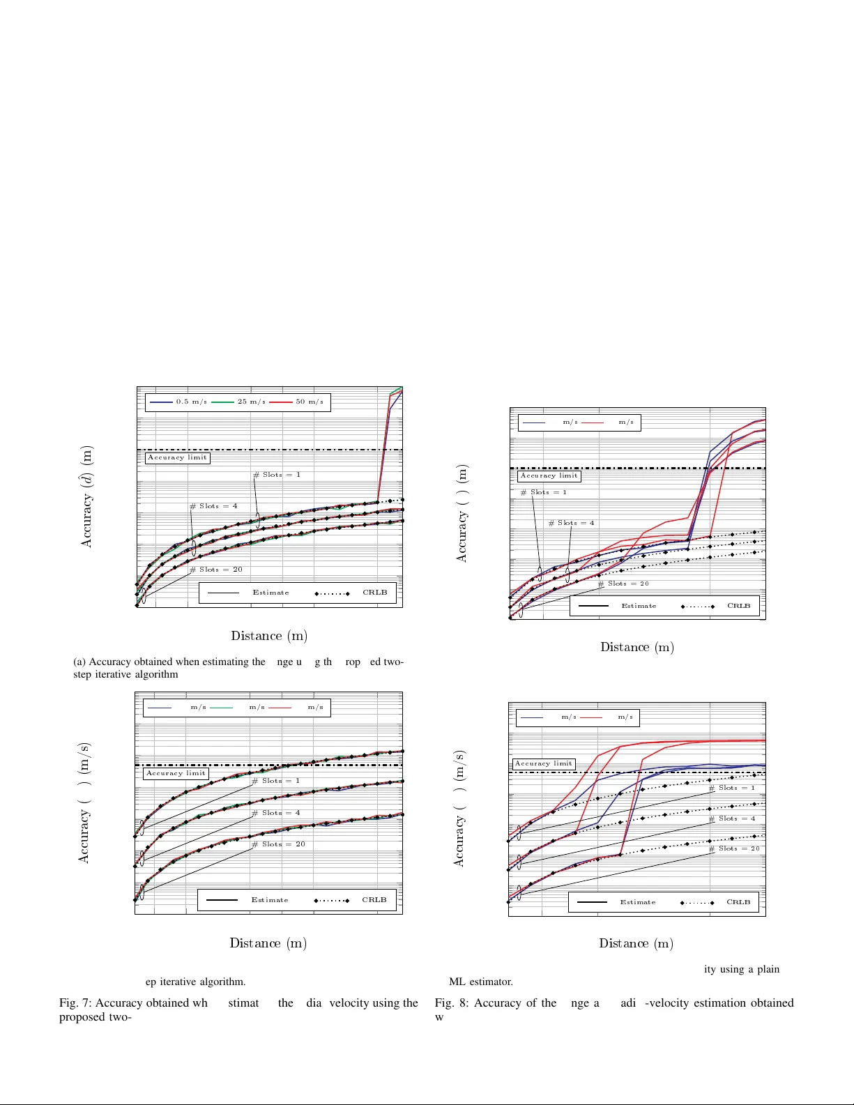
1 Inte grated sensing and communications in the 3GPP Ne w Radio: sensing limits Santiago Fernández, Javier Giménez, Mari Carmen Aguayo-T orres, José A. Cortés Communications and Signal Processing (ComSP) Lab, T elecommunication Research Institute (TELMA), Uni versidad de Málaga, E.T .S. Ingeniería de T elecomunicación, Bulev ar Louis P asteur 35, 29010 Málaga (Spain) {sf f, jgimenezdlc, mdaguayo, jca}@uma.es Abstract —Integrated Sensing and Communications (ISA C) is regarded as a key element of the bey ond–fifth-generation (5G) and sixth-generation (6G) systems, raising the question of whether current 5G New Radio (NR) signal structures can meet the sensing accuracy requir ements specified by the Third Generation Partnership Project (3GPP). This paper addresses this issue by analyzing the fundamental limits of range and velocity estimation through the Cramér–Rao lower bound (CRLB) f or a monostatic unmanned aerial vehicle (U A V) sensing use case currently under consideration in the 3GPP standardization process. The study focuses on standardized signals and also e valuates the potential performance gains achievable with reference signals specifically designed for sensing purposes. The compact CRLB expressions derived in this work highlight the fundamental trade-offs between estimation accuracy and sys- tem parameters. The r esults further indicate that inf ormation from multiple slots must be exploited in the estimation process to attain the performance targets defined by the 3GPP . As a result, the 5G NR positioning r eference signal (PRS), whose patterns may be suboptimal for velocity estimation when using single-slot resour ces, becomes suitable when multislot estimation is employed. Finally , we propose a two-step iterative range and radial-velocity estimator that attains the CRLB over a significantly wider range of distances than con ventional maximum-likelihood (ML) estimators, for which the well-known threshold effect sever ely limits the distance range over which the accuracy requir ements imposed by the 3GPP are satisfied. Index T erms —5G, 6G, Integrated sensing and communications (ISA C), accuracy , distance and speed estimation, Cramér -Rao lower bound (CRLB), maximum likelihood estimation. I . I N T RO D U C T I O N Integrated Sensing and Communications (ISAC) has emerged as a key paradigm in the ev olution tow ards beyond-fifth gener- ation (5G) and sixth generation (6G) systems, enabling wireless networks to jointly provide communication services and en vi- ronmental a wareness [ 1 ]. In this conte xt, sensing refers to the ca- pability of extracting information about the en vironment—such as the presence, distance, and velocity of targets—by processing reflected radio signals. Hence, the distance and speed of a target can be estimated by measuring the delay and the Doppler shift of the line-of-sight echo between the transmitter and the object [ 2 ]. This dif fers from the positioning functionality currently defined in 5G, where the base station (BS) transmits a reference signal that is used by the user equipment (UE) to estimate its position (which is reported back to the BS). The sensing functionality inherently combines detection and parameter estimation, and its performance is typically characterized in terms of both reliability and estimation accuracy . The inte gration of sensing into cellular systems enables a wide range of applications [ 3 ] [ 4 ]. On the one hand, sensing as a service allo ws the network to pro vide en vironmental information to external systems, such as autonomous vehicles or smart infrastructure. On the other hand, sensing can be leveraged to improv e network operation itself, enabling functionalities such as blockage detection, beam management, and proacti ve resource allocation. Howe ver , these benefits come at the cost of a fundamental trade-off between sensing performance and resource utilization, since sensing requires the allocation of time-frequency resources that would otherwise be used for communication. From a system perspecti v e, sensing can be implemented under two dif ferent operational modes: monostatic and bistatic [ 2 ]. In the former, the signal is recei ved and analyzed by the same BS, while in the bistatic case the signal is transmitted by a BS and receiv ed and analyzed by a different one. Monostatic operation simplifies synchronization and geometry but requires in-band full-duplex capabilities with stringent self-interference cancel- lation [ 5 ]. Bistatic (or multi-static, in case the signal is receiv ed by more than one BS) configurations relax this requirement but introduce additional complexity in terms of synchronization, coordination, and error propagation across distributed nodes. W ithin the Third Generation Partnership Project (3GPP) framew ork, sensing is being activ ely in vestigated as part of the ev olution towards 6G, of which sensing is considered a day- zer o functionality . The initial study item has defined a use case consisting on unmanned aerial vehicle (UA V) sensing using a monostatic configuration [ 6 ]. It has defined detection metrics, such as missed detection and false alarm probabilities, as well as estimation accuracy metrics for parameters such as target distance and velocity , which must remain below predefined thresholds with a 90% confidence lev el. A key open question is whether existing 5G NR signal structures are fundamentally capable of meeting these sensing accuracy requirements. Since the achiev able estimation perfor- mance is inherently limited by the structure of the transmitted signals and the allocated resources, it is essential to assess these limits from a theoretical perspectiv e before considering specific estimation algorithms. The Cramér -Rao lower bound (CRLB) provides a fundamen- tal benchmark for range and velocity estimation. While widely employed in inte grated sensing and communications (ISA C) applications [ 7 ]–[ 11 ], existing e xpressions consider neither the specific structure of 5G new radio (NR) signals nor the studied 2 use case [ 7 ], [ 8 ], [ 11 ], rely on channel models that yield ov erly complex expressions e valuable only numerically [ 11 ], or model the Doppler as a frequenc y shift rather than as the actual spectral compression/expansion [ 10 ]. In this work, we deriv e the CRLB for the U A V distance and velocity estimation under different 5G NR-based grid configura- tions, including standardized positioning reference signal (PRS) patterns and nov el sensing-oriented designs. The presented CRLB values are employed to compute the highest accuracy that can be obtained in the estimation of the range and v elocity , which are compared to the limits currently agreed in [ 12 ]. This provides insights into the fundamental trade-offs between estimation accuracy and resource utilization, and identifies the conditions under which the target sensing performance can be achiev ed. Furthermore, we propose a two-step iterative range and velocity estimation algorithm which attains the CRLB in a much wider range of signal-to-noise ratio (SNR) than plain max- imum likelihood (ML) approaches, whose threshold effect made them inadequate to comply with the imposed requirements. The rest of this paper is organized as follows. Section II describes the system model for the considered use case. Then, the CRLBs for velocity and range estimations are deriv ed in Section III . The different configurations for the sensing pattern are summarized in Section IV . In Section V , the proposed two-stage iterativ e range and velocity estimation algorithm is presented. Numerical results and discussion are presented in Section VI . Finally , conclusions are outlined in Section VII . I I . S Y S T E M M O D E L The considered use case consists of a monostatic configura- tion for U A V sensing, according to [ 6 ]. Since we are interested in obtaining an upper bound of the achiev able sensing perfor- mance, the case where only the target whose range and speed is to be estimated is present, as illustrated in Fig. 1 . The discrete-time lo w-pass equiv alent expression of an or- thogonal frequency-division multiplexing (OFDM) signal with N subcarriers and N cp samples of cyclic prefix can be expressed as x LP ( n ) = 1 N X m X k ∈K ( m ) X k,m e j 2 π N k ( n − N cp − mL ) × ω TX ( n − mL ) , (2) where X k,m is the constellation symbol carried by the k -th subcarrier in the m -th symbol, L = N + N cp is the number of samples per OFDM symbol and w TX ( n ) is a rectangular window of length L . The set of acti ve carriers used in the m -th OFDM symbol is denoted as K ( m ) . The signal x LP ( t ) is then con verted from digital to analog form, frequency-shifted to f c and con verted to a real one x ( t ) = √ 2 ℜ{ x LP ( t ) e j 2 πf c t } , (3) where ℜ{·} denotes the real part. Target v (velocit y) d (range ) BS Transm itted OFDM signal Echo sign al v φ (radial ve locity) Fig. 1: Sensing use case consisting of a monostatic configuration and a single U A V. The signal x ( t ) is then reflected in the single sensing target (ST) located d meters a way from the BS and mo ving at a relati v e radial-velocity v ϕ = v cos( ϕ ) . Let us denote the scattering amplitude of the ST as S = | S | e j ϕ S , which is related to the radar cross section as σ RCS = | S | 2 , and that is assumed to be independent of the frequency and azimuth and elev ation angles. The propagation loss is modeled as free-space path loss, which assuming that the bandwidth of the transmitted signal is much smaller than the carrier frequency can be obtained as α L = ( c 0 4 π d f c ) 2 [ 13 , Sec. 4.10-2]. Defining α T = α L σ RCS , the receiv ed echo can be expressed as y ( t ) = √ 2 ℜ  √ α T x LP ( t − τ ( t )) e − j (2 πf c τ ( t ) − ϕ S ) e j 2 πf c t  + w ( t ) , (4) where w ( t ) is the noise at the recei v er and τ ( t ) = 2 d/c 0 + 2 v ϕ t/c 0 . For simplicity of notation, τ d = 2 d/c 0 is defined. Since the transmitter and the receiver are co-located, perfect carrier and sampling synchronization can be assumed. Denoting the sampling period by T s = 1 N ∆ f , the discrete-time low-pass equiv alent of the echo receiv ed at the BS can be written as in ( 1 ). In order to compensate for part of the echo delay , the receiv er is assumed to shift the discrete Fourier transform (DFT) window by τ R = n R T s seconds relative to the start of the transmitted symbol. Disregarding the intercarrier interference (ICI) caused by the Doppler effect and assuming that the propagation delay is smaller than the cyclic prefix duration, the constellation symbols receiv ed at subcarrier k in the m -th OFDM symbol are then giv en by Y q ,m = √ α T X q ,m e − j 2 πφ q,m ( τ d ,v ϕ ) + W q ,m , (5) y LP ( n ) = √ α T x LP ( n − τ ( t ) /T s ) e − j (2 πf c τ ( t ) − ϕ S ) e j 2 πf c T s n + w LP ( n ) = √ α T N X m X k ∈K ( m ) X k,m e j 2 πk N  n − τ d T s − 2 v ϕ n c 0 − mL − N cp  e − j  2 π f c  τ d + 2 v ϕ nT s c 0  − ϕ S  ω TX  T s  n − mL − τ d T s − 2 v ϕ n c 0  + w LP ( n ) . (1) 3 where the noise sample in the q -th subcarrier of the m -th OFDM symbol is modeled as W q ,m ∼ C N  0 , σ 2 w  , and φ q ,m ( τ d , v ϕ ) = f c τ d − ϕ S 2 π | {z } ψ +∆ f q ( τ d − τ R ) + ( f c + ∆ f q ) 2 v ϕ c 0 δ m T s , (6) where ∆ f is the subcarrier spacing (SCS) and δ m =  n R + N cp + N − 1 2 + mL  . The phase in ( 6 ) consists of three terms: two that depend on τ d and one that depends on v ϕ . Our goal is to estimate the distance to the ST and its radial-velocity from the information embedded in this phase term. In practice, no information about τ d can be extracted from the phase term f c τ d because the product f c τ d ≫ 1 , which causes phase ambiguity . Accordingly , both f c τ d and ϕ S are grouped in the unknown parameter ψ . It is worth to highlight that expression ( 6 ) differs from the widely used one gi v en in [ 14 ]. In the latter , the phase shift associated to the radial speed, v ϕ , is independent of ∆ f q . This is due to the more accurate modeling of the Doppler effect used in ( 1 ), which causes a compression or expansion of the signal in addition to the frequency shift considered in [ 14 ]. I I I . C R A M E R - R AO L O W E R B O U N D O F R A N G E A N D V E L O C I T Y Let us now determine the CRLB of the range and radial- velocity estimation from a set of OFDM symbols with index es m ∈ M , with M = |M| . T o this end, it can be firstly observed that Y q ,m ∼ C N  √ α T X q ,m e − j 2 πφ q,m ( τ d ,v ϕ ) , σ 2 w  . Since noise samples in different subcarriers and OFDM symbols are inde- pendent, the log-lik elihood function (LLF) can be expressed as in ( 9 ) and the Fisher information as in ( 10 ), where it has been assumed that the constellation symbols of the sensing signals ha ve equal amplitude, | X q ,m | 2 = E X . Denoting the SNR in the q -th subcarrier as SNR q = α T E X /σ 2 w , the elements I ij = [ I ( τ d , v ϕ , ψ )] i,j are giv en by I 11 = X m ∈M X q ∈K ( m ) SNR q (∆ f q ) 2 I 12 = I 21 = 2 T s c 0 X m ∈M X q ∈K ( m ) SNR q ∆ f q ( f c + ∆ f q ) δ m I 13 = I 31 = X m ∈M X q ∈K ( m ) SNR q ∆ f q I 22 =  2 T s c 0  2 X m ∈M X q ∈K ( m ) SNR q ( f c + ∆ f q ) 2 δ 2 m I 23 = I 32 = 2 T s c 0 X m ∈M X q ∈K ( m ) SNR q ( f c + ∆ f q ) δ m , I 33 = X m ∈M X q ∈K ( m ) SNR q . (7) The CRLB for the estimation of d and v ϕ can then be expressed as V AR ( ˆ d ) ≥ c 2 0 32 π 2 I 22 I 33 − I 2 23 det ( I ( τ d , v ϕ , ψ )) V AR ( ˆ v ϕ ) ≥ 1 8 π 2 I 11 I 33 − I 2 13 det ( I ( τ d , v ϕ , ψ )) , (8) where det ( · ) denotes the determinant operator . Assuming that all subcarriers experience the same SNR, SNR q = SNR, that f c ≫ ∆ f q , and that all symbols use the whole set of acti ve subcarriers for sensing purposes, K ( m ) = K , the CRLB can be compactly written as V AR ( ˆ d ) ≥ Γ · 1 ∆ f 2 · 1 1 N A P q q 2 − ( 1 N A P q q ) 2 V AR ( ˆ v ϕ ) ≥ Γ · N 2 · ∆ f 2 f c · 1 1 M P m δ 2 m − ( 1 M P m δ m ) 2 , (11) with Γ = c 2 0 32 π 2 · SNR · M · N A . (12) As expected, the CRLB of both range and radial-velocity improv es with the SNR and the number of observations M · N A . Howe v er , while increasing the SCS, ∆ f , improves the range estimation, it degrades the radial-velocity one. Increasing the carrier frequency improves the velocity estimation without af- fecting the range one. Interestingly , range and radial-velocity estimation improve with increasing subcarrier and symbol index variance, respectiv ely , consistent with [ 15 ]. The CRLBs in ( 11 ) express the upper bound of the estimation process in terms of the variance. Ho we ver , 3GPP has agreed to use accuracy for a giv en confidence level as key performance indicator (KPI) [ 6 ]. Both magnitudes can be related as follows. The accurac y of an estimator ˆ θ for a confidence level (1 − α ) ( α is the significance le vel), is defined as the value of ∆ θ that fulfills P r  | ˆ θ − θ | ≤ ∆ θ  = 1 − α. (13) Assuming that ˆ θ is normally distributed with variance and bias V AR ( ˆ θ ) and B ( ˆ θ ) , respectiv ely 1 , ( 13 ) can be expressed in terms of the Gaussian Q-function, Q ( · ) , as 1 − α = 1 − Q   ∆ θ − B ( ˆ θ ) q V AR ( ˆ θ )   − Q   ∆ θ + B ( ˆ θ ) q V AR ( ˆ θ )   , (14) from which ∆ θ can be obtained. I V . S E N S I N G PA T T E R N S A. Full-slot The upper bound in the sensing performance is attained when all acti ve subcarriers of all the OFDM symbols in the slot are employed for this purpose. This signal pattern will be hereafter referred to as full-slot. The number of activ e subcarriers, N A , is smaller than the total number of subcarriers ( N A < N ), 1 While the CRLB is derived for unbiased estimators, we herein provide the relation for the general case of a biased estimator . 4 Λ( τ d , v ϕ , ψ ) = − X m ∈M X q ∈K ( m ) 1 σ 2 w  | Y q ,m | 2 + α T E X + ln  π σ 2 w  + 2 √ α T σ 2 w X m ∈M X q ∈K ( m ) ℜ n X q ,m e j 2 πφ q,m ( τ d ,v ϕ ) Y ∗ q ,m o . (9) I ( τ d , v ϕ , ψ ) =       − E h ∂ 2 Λ( τ d ,v ϕ ,ψ ) ∂ τ 2 d i − E h ∂ 2 Λ( τ d ,v ϕ ,ψ ) ∂ τ d ∂ v ϕ i − E h ∂ 2 Λ( τ d ,v ϕ ,ψ ) ∂ τ d ∂ ψ i − E h ∂ 2 Λ( τ d ,v ϕ ,ψ ) ∂ v ϕ ∂ τ d i − E h ∂ 2 Λ( τ d ,v ϕ ,ψ ) ∂ v 2 ϕ i − E h ∂ 2 Λ( τ d ,v ϕ ,ψ ) ∂ v ϕ ∂ ψ i − E h ∂ 2 Λ( τ d ,v ϕ ,ψ ) ∂ ψ∂ τ d i − E h ∂ 2 Λ( τ d ,v ϕ ,ψ ) ∂ ψ∂ v ϕ i − E h ∂ 2 Λ( τ d ,v ϕ ,ψ ) ∂ ψ 2 i       . (10) as defined in [ 16 ], where the maximum number of resource blocks (RBs) is determined by the signal bandwidth. The set of subcarrier indices is then giv en by K ( m ) = K =  − N A 2 , . . . , N A 2 − 1  . (15) B. P ositioning refer ence signal (PRS) The 5G NR standard defines a set of do wnlink reference signals for different purposes. Among the most representative are the synchronization signal (SS), which enables the UE to detect a cell; the demodulation reference signal (DM-RS), used for downlink channel estimation; the channel state information reference signal (CSI-RS), used to assess link quality; and the PRS, which allo ws the UE to estimate time-of-arri v al, typically using PRSs from multiple BSs [ 17 ], [ 18 ]. Among the reference signals, the PRS has important advantages for downlink sensing purposes, such as higher flexibility and density (as it admits multiple configurations) and being an always-on signal. The mapping of PRS symbols onto the physical resource grid is primarily go verned by the comb size , denoted as K PRS comb ∈ { 2 , 4 , 6 , 12 } , which specifies the spacing between subcarriers allocated to PRS within each RB. For instance, K PRS comb = 4 implies that one out of every four subcarriers within an OFDM symbol carries PRS. The corresponding time–frequency indices of the PRS pattern { q , m } are defined as m = m PRS start , . . . , m PRS start + M PRS − 1 , q = l · K PRS comb +  ( q PRS offset + q ′ ) mo d K PRS comb  , l = 0 , 1 , . . . , L PRS − 1 , (16) where M PRS ∈ { 1 , 2 , 4 , 6 , 12 } denotes the number of OFDM symbols within a slot allocated to PRS, q PRS offset ∈ { 0 , . . . , K PRS comb − 1 } is the frequenc y of fset, and L PRS = N A /K PRS comb is the number of PRS repetitions across frequency . Only the following combinations of { M PRS , K PRS comb } are supported in the specification, { M PRS , K PRS comb } ∈  { 1 , 2 } , { 2 , 2 } , { 4 , 2 } , { 6 , 2 } , { 12 , 2 } , { 1 , 4 } , { 4 , 4 } , { 12 , 4 } , { 1 , 6 } , { 6 , 6 } , { 12 , 6 } , { 1 , 12 } , { 12 , 12 }  . (17) Howe v er , in order to k eep the ov erhead constant among configu- rations, only the cases in which K PRS comb = M PRS are employed. The index q ′ in ( 16 ) depends on the relativ e symbol index ( m − m PRS start ) and K comb , as summarized in T able I . T ABLE I: V alue of q ′ for a gi ven ( m − m PRS start ) and K PRS comb K PRS comb Relativ e index of the m -th symbol within the time slot ( m − m PRS start ) 0 1 2 3 4 5 6 7 8 9 10 11 2 0 1 0 1 0 1 0 1 0 1 0 1 4 0 2 1 3 0 2 1 3 0 2 1 3 6 0 3 1 4 2 5 0 3 1 4 2 5 12 0 6 3 9 1 7 4 10 2 8 5 11 For illustrati ve purposes, Fig. 2 depicts example patterns corresponding to the four possible comb sizes of the PRS within a slot. While only three RBs are shown, the PRS pattern cov ers the whole set of activ e carriers. For simplicity , it has been assumed that m PRS start = 0 and q PRS offset = 0 . Under these assumptions, the indices in ( 16 ) reduce to m = 0 , 1 , . . . , M PRS − 1 , q = q ′ + l · K PRS comb − N A 2 , l = 0 , 1 , . . . , L PRS − 1 , (18) where the additional term − N A 2 centers the subcarrier indices around zero. As seen, each OFDM symbol m is associated with a distinct subset of PRS subcarriers, K ( m ) . C. DDRS Since PRS signals where not designed for sensing purposes, they hav e some drawbacks when used for this application. For instance, each carrier is used only once in each time slot, which hinders speed estimation. Similarly , for K PRS comb = 2 , the two symbols used in each time slot are consecuti ve, which also yields poor performance when speed is estimated using the PRS resources of a single slot. This can be explained in terms of the CRLB in ( 11 ), where the v ariance of the symbol indices used in the estimation is extremely small. T o assess whether better sensing performance may be ob- tained with specially designed patterns, we here propose a new reference signal, which will be referred to as Doppler- delay reference signal (DDRS), to which the follo wing design constraint are imposed. First, it must have a regular grid, using the same resource elements (REs) in all OFDM symbols. Hence, the employed frequenc y and time comb sizes, K DDRS comb and M DDRS comb respectiv ely , differ from those used in PRS. Second, the spacing between symbols with DDRS resources should be 5 0 1 2 3 4 5 6 7 8 9 10 11 12 13 OFD M S ymbol 0 1 2 3 4 5 6 7 8 9 10 11 12 13 14 15 16 17 18 19 20 21 22 23 24 25 26 27 28 29 30 31 32 33 34 35 36 S ub carrie r (a) K PRS comb = 2 . 0 1 2 3 4 5 6 7 8 9 10 11 12 13 OFD M S ymbol 0 1 2 3 4 5 6 7 8 9 10 11 12 13 14 15 16 17 18 19 20 21 22 23 24 25 26 27 28 29 30 31 32 33 34 35 36 S ub carrie r (b) K PRS comb = 4 . 0 1 2 3 4 5 6 7 8 9 10 11 12 13 OFD M S ymbol 0 1 2 3 4 5 6 7 8 9 10 11 12 13 14 15 16 17 18 19 20 21 22 23 24 25 26 27 28 29 30 31 32 33 34 35 36 S ub carrie r (c) K PRS comb = 6 . 0 1 2 3 4 5 6 7 8 9 10 11 12 13 OFD M S ymbol 0 1 2 3 4 5 6 7 8 9 10 11 12 13 14 15 16 17 18 19 20 21 22 23 24 25 26 27 28 29 30 31 32 33 34 35 36 S ub carrie r (d) K PRS comb = 12 . Fig. 2: Example of PRS patterns with the same o verhead. The green resource elements are the ones for sensing, the orange ones are used for other purposes. equally (or almost) spaced. Finally , DDRS must hav e the same ov erhead as the PRS. Denoting the number of OFDM symbols per time slot as M TS OFDM , the time–frequency indices of the DDRS patterns { q , m } are given by m = m DDRS start + ℓM DDRS comb , ℓ = 0 , 1 , . . . , M DDRS − 1 , q = l · K DDRS comb , l = 0 , 1 , . . . , L DDRS − 1 , (19) where M DDRS comb =  M TS OFDM K DDRS comb  , with ⌊·⌋ corresponding to the floor operation, L DDRS = N A /K DDRS comb is the number of DDRS repetitions across frequenc y and M DDRS ∈ { 2 , 4 , 6 , 7 , 12 , 14 } denotes the number of OFDM symbols within a slot allocated to DDRS. In order to keep the ov erhead constant and equal to the PRS cases, the follo wing configurations, denoted as { M DDRS , K DDRS comb } , are supported, { M DDRS , K DDRS comb } ∈  { 2 , 2 } , { 4 , 4 } , { 6 , 6 } , { 7 , 7 } , { 12 , 12 } , { 14 , 14 }  , (20) Fig. 3 sho ws the defined DDRS patterns. All configurations hav e the same overhead as the ones of the PRSs in Fig. 2 : 7.14%. 0 1 2 3 4 5 6 7 8 9 10 11 12 13 OFD M S ymbol 0 1 2 3 4 5 6 7 8 9 10 11 12 13 14 15 16 17 18 19 20 21 22 23 24 25 26 27 28 29 30 31 32 33 34 35 S ub carrie r (a) { M DDRS , K DDRS comb } = { 2 , 2 } . 0 1 2 3 4 5 6 7 8 9 10 11 12 13 OFD M S ymbol 0 1 2 3 4 5 6 7 8 9 10 11 12 13 14 15 16 17 18 19 20 21 22 23 24 25 26 27 28 29 30 31 32 33 34 35 S ub carrie r (b) { M DDRS , K DDRS comb } = { 4 , 4 } . 0 1 2 3 4 5 6 7 8 9 10 11 12 13 OFD M S ymbol 0 1 2 3 4 5 6 7 8 9 10 11 12 13 14 15 16 17 18 19 20 21 22 23 24 25 26 27 28 29 30 31 32 33 34 35 S ub carrie r (c) { M DDRS , K DDRS comb } = { 6 , 6 } . 0 1 2 3 4 5 6 7 8 9 10 11 12 13 OFD M S ymbol 0 1 2 3 4 5 6 7 8 9 10 11 12 13 14 15 16 17 18 19 20 21 22 23 24 25 26 27 28 29 30 31 32 33 34 35 S ub carrie r (d) { M DDRS , K DDRS comb } = { 7 , 7 } . 0 1 2 3 4 5 6 7 8 9 10 11 12 13 OFD M S ymbol 0 1 2 3 4 5 6 7 8 9 10 11 12 13 14 15 16 17 18 19 20 21 22 23 24 25 26 27 28 29 30 31 32 33 34 35 S ub carrie r (e) { M DDRS , K DDRS comb } = { 12 , 12 } . 0 1 2 3 4 5 6 7 8 9 10 11 12 13 OFD M S ymbol 0 1 2 3 4 5 6 7 8 9 10 11 12 13 14 15 16 17 18 19 20 21 22 23 24 25 26 27 28 29 30 31 32 33 34 35 S ub carrie r (f) { M DDRS , K DDRS comb } = { 14 , 14 } . Fig. 3: Patterns of the proposed DDRS signal for sensing purposes. It is worth noting that the configurations { 12 , 12 } and { 14 , 14 } hav e the same symbol separation, M DDRS comb = 1 , but the latter occupies all the symbols within a slot. The same applies to the configurations { 6 , 6 } and { 7 , 7 } , where M DDRS comb = 2 , although the latter does not cover all the symbols within the slot. V . R A N G E A N D V E L O C I T Y M L E S T I M A T O R S In this section we deriv e range and speed estimators for the signal in ( 5 ) and the full-slot sensing pattern, hence, K ( m ) = K . Since the range and velocity information is embedded in the phase of the receiv ed constellation symbol, let us define Z q ,m = Y ∗ q ,m X q ,m = √ α T E X e j 2 πφ q,m ( τ d ,v ϕ ) + W ′ q ,m , (21) 6 with φ q ,m ( τ d , v ϕ ) as giv en in ( 6 ) and W ′ q ,m = X q ,m W ∗ q ,m . In order to estimate the radial-velocity , it can be observed that φ q ,m ( τ d , v ϕ ) can be expressed as φ q ,m ( τ d , v ϕ ) = f v ϕ m + β q , (22) where f v ϕ = ( f c + ∆ f q ) 2 v ϕ c 0 LT s . β q = ∆ f q ( τ d − τ R ) + ( f c + ∆ f q ) 2 v ϕ c 0  n R + N cp + N − 1 2  T s + ψ . (23) Since v ϕ can be positiv e or negati ve, the span of nor- malized frequencies that can be unambiguously determined is f v ϕ ∈ [ − 1 / 2 , 1 / 2) . Hence, assuming that f c ≫ ∆ f N A / 2 , the range of v elocities that can be estimated unambiguously is v ϕ ∈ [ − v max ϕ , v max ϕ ) , with v max ϕ = c 0 N ∆ f 4 f c L . (24) The ML estimator of f v ϕ from Z q ,m , assuming that both α T and β q are unknown, can be obtained as in [ 19 , Eq. (7.66)]. These N A estimates, one for each q ∈ [ − N A / 2 , N A / 2 − 1] , can then be av eraged to obtain a single estimate of v ϕ . Howe ver , the estimates obtained with this procedure suffer from the well- known threshold ef fect [ 20 ], which severely limits the range of SNR v alues over which it attains the CRLB. T o extend this range, the noise has to be reduced before the estimation. The following two-step iterative process can be employed to achiev e this end. First, a coarse estimate of the radial-velocity , ˆ v c ϕ , is obtained from the frequency-av eraged value of Z q ,m as Z c m = 1 N A N A / 2 − 1 X q = − N A / 2 Z q ,m = √ α T E X 1 N A sin( π γ τ d N A ) sin( π γ τ d ) | {z } D N A (2 π γ τ d ) × e j 2 π  F c v ϕ m + η c  + W c m , (25) where W c m ∼ C N (0 , σ 2 w / N A ) , D N A ( x ) denotes the Dirichlet kernel with argument γ τ d = ∆ f  τ d − τ R + 2 v ϕ c 0 δ m T s  , (26) and where the frequency F c v ϕ and η c are giv en by F c v ϕ = 2 v ϕ c 0 LT s  f c − ∆ f 2  , η c =  f c − ∆ f 2  ×  τ d + 2 v ϕ c 0  n R + N cp + N − 1 2  T s  + ∆ f τ R / 2 − ϕ S 2 π . (27) A coarse estimate of the radial-velocity , ˆ v c ϕ , is then obtained by firstly computing the ML estimate of F v ϕ ( η c is unkno wn) as [ 19 , Eq. (7.66)] ˆ F c v ϕ = argmax f         M − 1 X m =0 Z c m e − j 2 πf m      2    , (28) which can be implemented by means of a DFT-based peri- odogram and a subsequent fine search using a numerical method [ 21 ], and then computing ˆ v c ϕ = ˆ F c v ϕ c 0 2( f c − ∆ f / 2) LT s . (29) Since the noise variance in Z c m is N A times lower than in Z q ,m , the threshold effect is displaced to lo wer SNR v alues by 10 log 10 ( N A ) (dB). Howe v er , the amplitude of Z c m depends on the range of the ST by means of the Dirichlet kernel D N A (2 π γ τ d ) . This makes the actual SNR in ( 25 ) to vary periodically with the range of the ST. This problem will be corrected in the second phase of the algorithm. Next, the coarse estimate of the range, ˆ d c is obtained. T o this end, the terms associated to the radial-velocity in Z q ,m are eliminated as H c q ,m = Z q ,m e − j 2 π ( f c +∆ f q ) 2 ˆ v ϕ c 0 δ m T s + W ′′ q ,m , (30) where W ′′ q ,m = X q ,m W ∗ q ,m e − j 2 π ( f c +∆ f q ) 2 ˆ v ϕ c 0 δ m T s . In order to mitigate the threshold effect in the range estimation, a time av eraging of H c q ,m is performed. Assuming perfect estimation of the radial-velocity , this yields H c q = 1 M M − 1 X m =0 H c q ,m = √ α T E X e j 2 πψ e j 2 π F c d z }| { ∆ f ( τ d − τ R ) q + W c q , (31) where W c q ∼ C N (0 , σ 2 w / M ) . The ML estimate of F c d is then obtained from the observ ations H c q as ˆ F c d = argmax f         N A − 1 X q =0 H c q e − j 2 πf q      2    , (32) and the coarse range estimate as ˆ d c = ˆ F c d ∆ f + τ R . (33) The range of the ST, d , is a positive v alue, so the span of nor- malized frequency , f , where the maximum of the periodogram in ( 32 ) can be determined without ambiguity is f ∈ [0 , 1) . In consequence, the maximum range that can be unambiguously estimated is giv en by d max = c 0 2  1 ∆ f + τ R  . (34) Now , in order to obtain a refined estimate of the radial- velocity , the range dependence in Z q ,m can be eliminated, which remov es the Dirichlet kernel that appeared in the averaging of Z q ,m performed to mitigate the threshold effect. T o this end, Z r m = 1 N A N A / 2 − 1 X q = − N A / 2 Z q ,m e − j 2 π ∆ f q (2 ˆ d c /c 0 − τ R ) = √ α T E X e j 2 π  F r v ϕ m + η r  + W r m , (35) The ML estimate of F r v ϕ is now computed analogously to ( 28 ), and a refined version of the radial-velocity , ˆ v r ϕ , is obtained as in ( 29 ). 7 Finally , a refined version of the range estimate, ˆ d r , is obtained. T o this end, the effect of v ϕ in Z q ,m is firstly compensated as in ( 30 ), yielding H r q ,m , whose time-av eraged value, H r q , is ob- tained as in ( 31 ). Finally , ˆ d r is obtained proceeding analogously to ( 32 ) and ( 33 ). Algorithm V .1 T wo-step iterative range and speed estimation algorithm First iteration 1: Compute Z q ,m from Y q ,m as in ( 21 ) 2: Calculate Z c m by averaging Z q ,m ov er the activ e subcarriers as in ( 25 ) 3: Obtain a coarse estimate of the radial-velocity , ˆ v c ϕ , from Z c m using ( 28 ) and ( 29 ) 4: Eliminate the velocity terms in φ q ,m ( τ d , v ϕ ) by computing H c q ,m as in ( 30 ) 5: Obtain a coarse estimate of the range, ˆ d c , from H c q in ( 31 ) using ( 32 ) and ( 33 ) Second iteration 6: Eliminate the range terms in Z q ,m and compute its time- av eraged v alue, Z r m , as in ( 35 ) 7: Obtain a refined estimate of the radial-velocity , ˆ v r ϕ , from Z r m analogously to ( 28 ) and ( 29 ) 8: Eliminate the velocity terms in φ q ,m ( τ d , v ϕ ) by comput- ing H r q ,m and obtaining its frequency-a veraged v alue, H r q , analogously to ( 31 ) 9: Obtain a refined estimate of the range, ˆ d , from H r q proceed- ing as in ( 32 ) and ( 33 ) As mentioned, the employed ML estimators in ( 28 ) and ( 32 ) can be implemented by means of a DFT and a subsequent refinement using a numerical method. The size of the DFT, denoted as N per , determines the resolution of the estimates, as the refinement is carried out around a normalized frequenc y con- strained to a discrete set. Since the span of F v ϕ ∈ [ − 1 / 2 , 1 / 2) and F d ∈ [0 , 1) is equally spaced di vided into N per points, i.e., ∆ F = 1 / N per , the following velocity and range resolutions are obtained under the assumption that f c ≫ ∆ f N A / 2 ∆ v ϕ = c 0 N ∆ f 2 f c N per L ∆ d = c 0 2 N per ∆ f . (36) V I . N U M E R I C A L R E S U LT S A N D D I S C U S S I O N This section shows the highest accuracy that can be achieved in the range and radial-speed estimation of an U A V using monostatic sensing. Ne xt, the suitability of the PRS for sensing purposes is e v aluated and compared against the performance of the proposed DDRS pattern, to assess whether the intro- duction of a ne w sensing-oriented reference signal is justified, or whether the improv ements reported for other seemingly better patterns are not practically significant. Finally , since the aforementioned results are obtained by means of the CRLB, but there is no guarantee that an ef ficient estimator can be obtained for the considered problem, we show that the performance giv en by the two-step iterative estimator proposed in Section V is efficient and compare it to the performance of a plain ML estimator . In all cases, the accuracy of the range and radial-velocity is obtained for estimators that use sensing resources from a number of slots ranging from 1 to 20. Increasing the number of slots used in the estimation improves performance at the cost of an increased complexity , in particular the memory required to store the complex values Y q ,m to be used by the estimator . A. System parameters This work uses the system parameters defined in [ 6 ] for the considered use case and that are summarized in T able II . T ABLE II: System parameters Parameter Description V alue µ Numerology index 1 f c Carrier frequency 4 GHz ∆ f SCS 30 kHz BW Channel bandwidth 100 MHz N Number of carriers 4096 N cp Cyclic prefix (samples) 288 samples T s Sampling period 8.14 ns N RB Number of activ e RBs 273 N A Number of activ e subcarriers 3276 The radar cross section (RCS) is modeled according to [ 22 , Sec. 7.9.2.1 (model 1)], which states that it can be expressed as the product of three terms, σ RCS = σ M σ D σ S , where σ M = − 12 . 81 dBsm is deterministic, σ D = 1 when it is independent of the angle of incidence, and σ S is a log-normal random variable such that 10 log ( σ S ) ∼ N ( µ σ S_dB , σ 2 σ S_dB ) , where the mean and the variance are related as µ σ S_dB = − ln (10) 20 σ 2 σ S_dB , (37) with σ σ S_dB = 3 . 74 dB for small U A Vs. The inter-BS distance of 500 m agreed in [ 6 ] is assumed, which leads to a maximum coverage distance of roughly 290 m. Since the ST can be up to 300 m abov e the BS, the maximum range is just below 420 m. Hence, the accuracy for STs located at a maximum distance of 440 m is e valuated. According to [ 23 ], a maximum speed of 50 m/s (180 km/h) is considered. The KPIs defined in [ 12 ] for the considered use case are giv en in T able III . Reg arding range accurac y , since the distance d considered in this work includes both horizontal and vertical components, a 10 m accuracy requirement is imposed on d to ensure compliance in all cases. Interestingly , the v alues in T able III limit the maximum number of slots that can be used in the estimation. For instance, in 400 slots (0.2 s), a ST moving at 50 m/s the ST has displaced 10 m (the accuracy limit) from its position. Fortunately , a lo wer number of slots is actually required to meet the requirements, as it will be shown. 8 B. Sensing resolution and maximum values Expressions ( 24 ) and ( 34 ) gav e the maximum radial-velocity and range values that can be unambiguously estimated, while expression ( 36 ) provided the resolution that can be achiev ed when estimating d and v ϕ using an N per -DFT. For illustrativ e purposes, T able IV reports the maximum unambiguous values for range and velocity obtained using the system parameters in T able II . Similarly , T able V provides the attainable resolution for different values of N per . Note that the indicated limit for range estimation corresponds to the scenario where τ R = 0 , i.e., frame synchronization is not performed. Otherwise, larger ranges can, in principle, be estimated without ambiguity . Howe ver , in practice the maximum range is constrained by the sensiti vity of the receiv er . C. Accur acy assessment First, accuracy v alues giv en by ( 14 ) using the variance gi ven by the CRLB in ( 11 ) for the full-slot pattern and the confidence lev els in T able III are presented. Fig. 4 sho ws the results obtained when the estimation is computed over 1, 2, 4, and 20 time slots. As seen, the distance accuracy requirement is easily satisfied with a single time slot, whereas at least two time slots are necessary to meet the velocity accuracy requirement. As expected, lower performance is obtained when using PRSs. Fig. 5 shows the accuracy bounds (deri ved from the CRLB) when the range and radial-velocity are estimated over the PRS resources from 1 , 4 and 20 time slots. It can be observed that a single time slot is more than sufficient to meet the distance accuracy requirement, howe ver , more than 4 time slots are now required to meet the velocity accuracy requirements. In practice, the performance is independent of T ABLE III: KPIs adopted for ev aluation purpose of NR ISAC. KPI Required accuracy and confidence lev el Horizontal Positioning 10 m with confidence level 90 % V ertical Positioning 10 m with confidence level 90 % V elocity 5 m/s with confidence level 90 % T ABLE IV: Maximum unambiguous v alues of the range and radial- velocity estimates for the system parameters in T able II . Magnitude Maximum value Range ( d max ) 4996.5 m V elocity ( v max ϕ ) 525.2 m/s T ABLE V: Resolution values of the range and radial-velocity estimates when using DFT-based estimators with N per samples and the system parameters in T able II . N per 16 256 4096 65536 ∆ d (m) 313.3 19.52 1.220 0.076 ∆ v ϕ (m/s) 65.6 4.10 0.256 0.016 100 200 300 400 10 − 4 10 − 3 10 − 2 10 − 1 10 0 10 1 10 2 10 3 Distance (m) A ccuracy ( ˆ d ) (m) # Slots = 1 # Slots = 2 # Slots = 4 # Slots = 20 A ccurac y lim it (a) Highest accuracy in range estimation. 100 200 300 400 10 − 4 10 − 3 10 − 2 10 − 1 10 0 10 1 10 2 10 3 Distance (m) A ccuracy ( ˆ v ϕ ) (m/s) # Slots = 1 # Slots = 2 # Slots = 4 # Slots = 20 A ccurac y lim it (b) Highest accuracy in radial-velocity estimation. Fig. 4: Maximum achiev able accuracy in range and radial-velocity estimations using the full-slot sensing pattern. K PRS comb when multiple time slots are employed. Howe ver , the accuracy strongly depends on the PRS pattern when a single time slot is used: the larger K PRS comb , the better the accuracy . The rationale for this behavior is that the radial-velocity information induces a phase shift in the received symbols, Y q ,m , which primarily varies with the symbol index m , as shown in ( 22 ), and the time extent of the PRS pattern increases with K PRS comb , as illustrates in Fig. 2 . This can also be explained in terms of the CRLB in ( 11 ), which shows that the performance improv es with increasing v ariance of the indices of the OFDM symbols used in the estimation, and the latter increases with K PRS comb . Now , the performance obtained with the proposed DDRS patterns is assessed. Fig. 6 depicts the accurac y bounds for the range and radial-velocity obtained when the DDRS re- sources in 1 , 4 and 20 time slots are used. As observed, similar accurac y le vels are obtained for all DDRS patterns. The configurations { M DDRS , K DDRS comb } = {{ 2 , 2 } , { 7 , 7 } , { 14 , 14 }} 9 provide slightly better radial-velocity accuracy when 4 and 20 time slots are considered. In contrast, for a single time slot, the configurations {{ 7 , 7 } , { 14 , 14 }} achie ve the best performance. Interestingly , obtained values are similar to the ones given by the PRSs when the estimation is performed using multiple time slots. When a single time slot is used, the range estimation accuracy is similar to that obtained with the PRSs, whereas the radial-velocity accuracy becomes almost independent of the DDRS pattern and matches the best-case performance of the PRS pattern obtained with K PRS comb = 12 . This result is in agreement with the CRLB in ( 11 ), since the variance of the symbol indices of the PRS is very small when a single time slot is employed, but similar to that of the DDRS when multiple slots are used. Since the accuracy values obtained from a single time slot are insufficient to meet the radial-velocity accuracy requirement in T able III , practical estimators have to resort to multiple slots. 100 200 300 400 10 − 4 10 − 3 10 − 2 10 − 1 10 0 10 1 10 2 10 3 # Slots = 1 # Slots = 4 # Slots = 20 Distance (m) A ccuracy ( ˆ d ) (m) K PRS comb = 2 K PRS comb = 4 K PRS comb = 6 K PRS comb = 12 A ccurac y lim it (a) Highest accuracy in range estimation. 100 200 300 400 10 − 4 10 − 3 10 − 2 10 − 1 10 0 10 1 10 2 10 3 # Slots = 1 # Slots = 4 # Slots = 20 Distance (m) A ccuracy ( ˆ v ϕ ) (m/s) K PRS comb = 2 K PRS comb = 4 K PRS comb = 6 K PRS comb = 12 A ccurac y lim it (b) Highest accuracy in radial-velocity estimation. Fig. 5: Maximum achiev able accuracy in range and radial-velocity estimations using dif ferent PRS sensing patterns. Hence, presented results suggest that defining a new reference signal for sensing purposes may be unnecessary when the 5G frame structure is employed. Accuracy values presented so far hav e been derived from the variance giv en by the CRLB. W e now prov e that the estimator proposed in Algorithm V .1 attains this bound ov er a wide range of distances. T o this end, Fig. 7 depicts the accurac y of the range and radial-velocity estimations obtained when the full- slot sensing pattern is employed. Presented values are computed from ( 14 ) using the bias and variance of the estimates obtained by means of Monte Carlo simulations. Results are shown for STs with different radial velocities and three observation sets ( 1 , 4 , and 20 time slots). As seen, the proposed estimator is efficient ov er the required range of distances (up to 420 m), except for the estimates obtained using a single time slot, for which the threshold effect limits the range over which the accuracy requirement is met to a maximum of 400 m. 100 200 300 400 10 − 4 10 − 3 10 − 2 10 − 1 10 0 10 1 10 2 10 3 # Slots = 1 # Slots = 4 # Slots = 20 Distance (m) A ccuracy ( ˆ d ) (m) A cc u rac y lim it { M DDRS , K DDRS comb } = { 2 , 2 } { M DDRS , K DDRS comb } = { 4 , 4 } { M DDRS , K DDRS comb } = { 6 , 6 } { M DDRS , K DDRS comb } = { 7 , 7 } { M DDRS , K DDRS comb } = { 12 , 12 } { M DDRS , K DDRS comb } = { 14 , 14 } (a) Highest accuracy in range estimation. 100 200 300 400 10 − 4 10 − 3 10 − 2 10 − 1 10 0 10 1 10 2 10 3 # Slots = 1 # Slots = 4 # Slots = 20 Distance (m) A ccuracy ( ˆ v ϕ ) (m/s) A ccurac y lim it { M DDRS , K DDRS comb } = { 2 , 2 } { M DDRS , K DDRS comb } = { 4 , 4 } { M DDRS , K DDRS comb } = { 6 , 6 } { M DDRS , K DDRS comb } = { 7 , 7 } { M DDRS , K DDRS comb } = { 12 , 12 } { M DDRS , K DDRS comb } = { 14 , 14 } (b) Highest accuracy in radial-velocity estimation. Fig. 6: Maximum achiev able accuracy in range and radial-velocity estimations using dif ferent DDRS sensing patterns. 10 Finally , to highlight the improv ement of the proposed two- step iterativ e estimator over plain ML ones, Fig. 8 shows the accuracy achieved by the latter , as defined in the paragraph immediately following ( 24 ), when using the full-slot sensing pattern. It can be observed that the threshold ef fect appears at short distances, prev enting the performance requirement from being met over the considered range. V I I . C O N C L U S I O N This work has determined the theoretical accuracy limits for range and velocity estimation of a single U A V using 5G signals within a monostatic sensing framew ork. The compact CRLB expressions derived herein highlight the fundamental trade-offs between estimation accuracy and system parameters. These variance bounds are then translated into accuracy values and compared with the requirements specified by the 3GPP. The 20 50 100 200 250 300 400 10 − 4 10 − 3 10 − 2 10 − 1 10 0 10 1 10 2 10 3 # Slots = 1 # Slots = 4 # Slots = 20 Distance (m) A ccuracy ( ˆ d ) (m) 0 . 5 m/s 25 m/s 50 m/s Estimate CRLB A ccuracy li mit (a) Accuracy obtained when estimating the range using the proposed two- step iterativ e algorithm. 20 50 100 200 250 300 400 10 − 4 10 − 3 10 − 2 10 − 1 10 0 10 1 10 2 10 3 # Slots = 1 # Slots = 4 # Slots = 20 Distance (m) A ccuracy ( ˆ v ϕ ) (m/s) 0 . 5 m/s 25 m/s 50 m/s Estimate CRLB A ccuracy li mit (b) Accuracy obtained when estimating the radial-velocity using the proposed two-step iterative algorithm. Fig. 7: Accuracy obtained when estimating the radial-velocity using the proposed two-step iterati ve algorithm and the full-slot sensing pattern. obtained results indicate that, when all the resources within a slot are used for sensing purposes, the estimator must exploit information from at least two slots to meet the accuracy limit for velocity estimation, whereas a single slot suffices to satisfy the accuracy requirement for range estimation. The accuracy achie ved using the 5G NR PRS, which is the most suitable standardized reference signal for sensing purposes, is also ev aluated and compared with that obtained using a reference signal specifically designed for sensing. The presented results show that, when estimation is performed ov er the PRS resources of a single slot, the most suitable PRS pattern is the one with a comb size equal to 12, K PRS comb = 12 . Ho wev er , negli- gible differences between patterns are observed when estimation is carried out o ver multiple slots. Furthermore, since it has also been sho wn that more than four slots are required to meet the radial-velocity accurac y requirements imposed by the 3GPP, in practice, this implies that the PRS yields nearly the same 20 50 100 200 250 10 − 4 10 − 3 10 − 2 10 − 1 10 0 10 1 10 2 10 3 # Slots = 1 # Slots = 4 # Slots = 20 Distance (m) A ccuracy ( ˆ d ) (m) 0 . 5 m/s 50 m/s Estimate CRLB A ccuracy li mit (a) Accuracy obtained when estimating the range using a plain ML estimator . 20 50 100 200 250 10 − 4 10 − 3 10 − 2 10 − 1 10 0 10 1 10 2 10 3 # Slots = 1 # Slots = 4 # Slots = 20 Distance (m) A ccuracy ( ˆ v ϕ ) (m/s) 0 . 5 m/s 50 m/s Estimate CRLB A cc u ra cy lim it (b) Accuracy obtained when estimating the radial-velocity using a plain ML estimator . Fig. 8: Accuracy of the range and radial-velocity estimation obtained with plain ML estimators and the full-slot sensing pattern. 11 accuracy as specifically designed signals, which outperform it in single-slot estimation. Although, in principle, there is no guarantee that a practical estimator attaining the CRLB can be designed, we propose a two-step iterative range and radial-v elocity estimator that is efficient o ver a significantly wider range of distances than con- ventional maximum-likelihood (ML) estimators. The presented results show that the latter are strongly af fected by the well- known threshold effect, which limits the distance range o ver which the accuracy requirements imposed by the 3GPP are satisfied to less than 200 m for range estimation and less than 130 m for radial-velocity estimation. R E F E R E N C E S [1] D. Zhang, Y . Cui, X. Cao, N. Su, Y . Gong, F . Liu, W . Y uan, X. Jing, J. An- drew Zhang, J. Xu, C. Masouros, D. Niyato, and M. Di Renzo, “Integrated sensing and communications over the years: An evolution perspective, ” IEEE Communications Surveys & T utorials , vol. 28, pp. 5014–5048, 2026. [2] H. Andersson, “Joint communication and sensing in 6G networks. ” Ericsson Blog, [On-line, 24/03/2026] https://www .ericsson.com/en/blog/2021/10/joint-sensing-and- communication-6g, 2021. [3] Y . Li, F . Liu, Z. Du, W . Y uan, and C. Masouros, “ISA C-Enabled V2I Networks Based on 5G NR: How Much Can the Overhead Be Reduced?, ” in IEEE International Conference on Communications W orkshops (ICC W orkshops) , pp. 691–696, 2023. [4] Y . Cui, J. Nie, and F . e. a. Liu, “Integrated sensing and commu- nication: T owards multifunctional perceptive network, ” arXiv pr eprint arXiv:2510.14358, 16/10/2025 , 2025. [5] J. A. Zhang, M. L. Rahman, K. W u, X. Huang, Y . J. Guo, S. Chen, and J. Y uan, “Enabling joint communication and radar sensing in mobile networks—a survey , ” IEEE Communications Surveys & T utorials , vol. 24, no. 1, pp. 306–345, 2022. [6] 3GPP TSG RAN WG1, “Summary #5 on Evaluations for NR ISAC RAN WG1 #122bis, Agenda Item 10.5.1, Moderator: Xiaomi, ” RAN WG1 Meeting Contribution R1-2507427, Third Generation Partnership Project (3GPP), Prague, Czech, Nov . 2025. https://www .3gpp.org/ftp/tsg_ ran/WG1_RL1/TSGR1_122b/Docs . [7] I. Bekkerman and J. T abrikian, “T arget detection and localization using MIMO radars and sonars, ” IEEE T ransactions on Signal Processing , vol. 54, no. 10, pp. 3873–3883, 2006. [8] L. Gaudio, M. Kobayashi, B. Bissinger, and G. Caire, “Performance Analysis of Joint Radar and Communication using OFDM and OTFS, ” in IEEE International Conference on Communications W orkshops (ICC W orkshops) , pp. 1–6, 2019. [9] F . Liu, Y .-F . Liu, A. Li, C. Masouros, and Y . C. Eldar, “Cramér-rao bound optimization for joint radar-communication beamforming, ” IEEE T r ansactions on Signal Pr ocessing , vol. 70, pp. 240–253, 2022. [10] Z. W ei, Y . W ang, L. Ma, S. Y ang, Z. Feng, C. Pan, Q. Zhang, Y . W ang, H. W u, and P . Zhang, “5G PRS-Based Sensing: A Sensing Reference Signal Approach for Joint Sensing and Communication System, ” IEEE T r ansactions on V ehicular T echnology , vol. 72, no. 3, pp. 3250–3263, 2023. [11] M. Soltani, M. Mirmohseni, and R. T af azolli, “On stochastic fundamental limits in a downlink integrated sensing and communication network, ” IEEE Tr ansactions on Communications , vol. 73, no. 11, pp. 10436–10450, 2025. [12] 3GPP TSG RAN WG1, “Summary #6 on Evaluations for NR ISAC RAN WG1 #123, Agenda Item 10.5.1, Moderator: Xiaomi, ” RAN WG1 Meeting Contrib ution R1-2509243, Third Generation Partnership Project (3GPP), Dallas, US, No v . 2025. https://www .3gpp.org/ftp/tsg_ran/WG1_ RL1/TSGR1_123/Docs . [13] J. G. Proakis and M. Salehi, Digital Communications . New Y ork, NY , USA: McGraw-Hill, 5th ed., 2008. [14] C. Sturm and W . Wiesbeck, “W a veform design and signal processing aspects for fusion of wireless communications and radar sensing, ” Pro- ceedings of the IEEE , vol. 99, no. 7, pp. 1236–1259, 2011. [15] X.-Y . W ang, S. Y ang, K. Meng, H.-Y . Zhai, and C. Masouros, “On the Fundamental Trade-Of fs of T ime-FrequencyResource Distribution in OFDMA ISA C, ” , 2024. [16] “Third Generation Partnership Project; T echnical Specification Group Radio Access Network; NR; Base Station (BS) radio transmission and reception (Release 19), ” 3GPP T echnical Specification TS 38.104, Third Generation Partnership Project (3GPP), June 2025. A vailable at https: //www .3gpp.org/ftp/Specs/archive/38_series/38.104/ . [17] “5G; NR; Physical channels and modulation, ” T echnical Specification TS 38.211, E.T .S.I., July 2025. A v ailable at https://portal.etsi.org/webapp/ workprogram/Report_W orkItem.asp?WKI_ID=75300 . [18] E. Dahlman, S. Parkvall, and J. Sköld, 5G NR: The Next Generation W ir eless Access T echnology . Elsevier , 2018. [19] S. M. Kay , Fundamentals of Statistical Signal Processing: Estimation Theory . USA: Prentice Hall, Inc., 1993. [20] A. Steinhardt and C. Bretherton, “Thresholds in frequency estimation, ” in IEEE International Conference on Acoustics, Speech, and Signal Pr ocessing , vol. 10, pp. 1273–1276, 1985. [21] D. Rife and R. Boorstyn, “Single tone parameter estimation from discrete- time observations, ” IEEE T ransactions on Information Theory , vol. 20, no. 5, pp. 591–598, 1974. [22] Third Generation P artnership Project (3GPP), “Study on channel model for frequencies from 0.5 to 100 GHz, ” T echnical Report TR 38.901 V19.1.0, 3GPP T echnical Specification Group Radio Access Network, Sept. 2025. (Release 19). [23] 3GPP TSG RAN WG1, “Summary #4 on Evaluations for NR ISAC RAN WG1 #122, Agenda Item 10.5.1, Moderator: Xiaomi, ” RAN WG1 Meeting Contrib ution R1-2506479, Third Generation Partnership Project (3GPP), Bengaluru, India, 2025. https://www .3gpp.org/ftp/tsg_ran/WG1_ RL1/TSGR1_122/Docs .