FI-KAN: Fractal Interpolation Kolmogorov-Arnold Networks

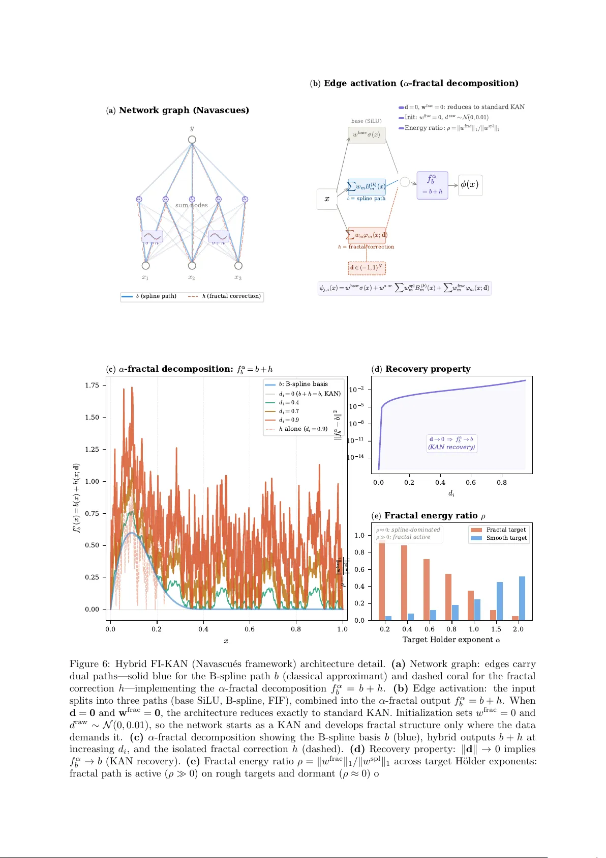
FI-KAN: F ractal In terp olation Kolmogoro v–Arnold Net w orks Gnank an Landry Regis N’guessan 1 , 2 , 3 1 Axiom Research Group 2 Dept. of Applied Mathematics and Computational Science, NM-AIST, Arusha, T anzania 3 AIMS Research and Inno v ation Cen tre, Kigali, Rwanda rnguessan@aimsric.org Abstract Kolmogoro v–Arnold Netw orks (KAN) emplo y B-spline bases on a ﬁxed grid, pro viding no intrinsic m ulti- scale decomp osition for non-smo oth function approximation. W e introduce F ractal Interpolation KAN (FI-KAN), which incorp orates learnable fractal interpolation function (FIF) bases from iterated function system (IFS) theory into KAN. Two v ariants are presen ted: Pure FI-KAN (Barnsley , 1986) replaces B-splines en tirely with FIF bases; Hybrid FI-KAN (Nav ascu´ es, 2005) retains the B-spline path and adds a learnable fractal correction. The IFS con traction parameters giv e eac h edge a diﬀerentiable fractal dimension that adapts to target regularit y during training. On a H¨ older regularit y b enc hmark ( α ∈ [0 . 2 , 2 . 0]), Hybrid FI-KAN outp erforms KAN at ev ery regularit y lev el (1 . 3 × to 33 × ). On fractal targets, FI-KAN achiev es up to 6 . 3 × MSE reduction o ver KAN, maintaining 4 . 7 × adv an tage at 5 dB SNR. On non-smooth PDE solutions ( scikit-fem ), Hybrid FI-KAN ac hieves up to 79 × impro vemen t on rough-co eﬃcient diﬀusion and 3 . 5 × on L-shap ed domain corner singularities. Pure FI-KAN’s complemen tary b eha vior, dominating on rough targets while underp erforming on smo oth ones, provides controlled evidence that basis geometry must matc h target regularit y . A fractal dimension regularizer provides interpretable complexity control whose learned v alues reco ver the true fractal dimension of eac h target. These results establish regularity-matc hed basis design as a principled strategy for neural function appro ximation. Keyw ords: Kolmogorov–Arnold Netw orks, fractal interpolation, iterated function systems, H¨ older regularity , function appro ximation, neural architecture design. Figure 1: MLPs vs. KANs vs. FI-KANs. (a) MLP: scalar weigh ts on edges, ﬁxed activ ations on no des. (b) KAN: learnable B-spline functions on edges. (c) Pure FI-KAN: replaces B-splines with fractal interpolation bases φ m ( x ; d ). (d) Hybrid FI-KAN: retains B-splines and adds a fractal correction ( f α b = b + h ). When d = 0 , (d) reduces to (b). 1 1 In tro duction Neural function appro ximation arc hitectures em bed implicit assumptions about the regularit y of their targets through their c hoice of basis functions. Multi-la yer perceptrons (MLPs) with smo oth activ ation functions (ReLU, SiLU, GELU) construct appro ximants in spaces of piecewise smo oth or analytic functions [ 11 , 20 ]. Kolmogoro v–Arnold Net w orks (KAN) [ 27 ], motiv ated b y the Kolmogorov–Arnold represen tation theorem [ 24 , 3 ], replace ﬁxed activ ations with learnable univ ariate functions parameterized as B-spline expansions [ 13 ]. B-splines of order k repro duce polynomials of degree at most k − 1 and pro vide near-optimal appro ximation rates for targets in Sob olev and Beso v spaces with in teger or high fractional smo othness. Ho wev er, many functions of scientiﬁc and engineering interest are not smo oth. T urbulence v elo cit y ﬁelds, ﬁnancial time series, fracture surfaces, natural terrain proﬁles, and biomedical signals with m ulti-scale oscillations all exhibit non-trivial H¨ older regularit y , fractal self-similarit y , or no where-diﬀerentiable character. F or such targets the smo oth basis functions used by both MLPs and KANs are fundamentally mismatc hed: appro ximating a function with b o x-coun ting dimension dim B > 1 using a smooth basis at resolution h requires O ( h − 1 /α ) basis elements (where α is the H¨ older exp onen t), with no gain from the polynomial repro duction properties that make splines eﬃcient for smo oth targets. This pap er introduces F ractal In terp olation KAN (FI-KAN), which augmen ts or replaces the B-spline bases in KAN with fractal interpolation function (FIF) bases derived from iterated function system (IFS) theory [ 5 , 21 ]. The key inno v ation is that the vertical contraction parameters { d i } of the IFS are treated as trainable parameters, giving each edge activ ation a diﬀer entiable fr actal dimension that adapts to the regularit y structure of the target function during training. Con tributions. 1. Tw o arc hitectures grounded in fractal approximation theory . Pur e FI-KAN (Barnsley framew ork) replaces B-splines en tirely with FIF bases. Hybrid FI-KAN (Na v ascu´ es framework) retains B-splines and adds a fractal correction path. Both architectures are deriv ed from classical mathematical framew orks, not ad hoc mo diﬁcations. 2. Learnable fractal dimension. The contraction parameters provide a contin uous, diﬀerentiable knob from smo oth (piecewise linear, dim B = 1) to rough (fractal, dim B > 1) basis functions, learned from data. 3. F ractal dimension regularization. A diﬀeren tiable regularizer p enalizes unnecessary fractal complexit y , implementing Occam’s razor at the lev el of function geometry rather than parameter coun t. 4. Comprehensiv e exp erimen tal v alidation. Across functions spanning the H¨ older regularity sp ectrum, FI-KAN demonstrates that matc hing basis regularit y to target regularity yields substantial appro ximation gains on non-smo oth targets, with additional adv antages in noise robustness and con tinual learning. 5. Empirical v alidation of the regularit y-matc hing h yp othesis. The contrast b et ween Pure and Hybrid FI-KAN pro vides controlled evidence that the geometric structure of the basis functions, not merely their n umber, is a critical design v ariable. 6. V alidation on non-smooth PDE solutions. On reference solutions computed via scikit-fem [ 18 ] for elliptic PDEs with corner singularities (H¨ older 2 / 3) and rough co eﬃcients generated by fractional Bro wnian motion ( fbm pac k age [ 16 ]), Hybrid FI-KAN achiev es 65–79 × impro vemen t ov er KAN, demonstrating that the regularity-matc hing adv an tage extends to structured roughness inherited from PDE op erators. Scop e. W e do not claim FI-KAN as a general-purp ose replacement for KAN. W e claim it as a principled extension for function classes with non-trivial geometric regularit y , supported b y b oth theory and exp erimen t. On smooth targets where B-splines are near-optimal, the Hybrid v ariant remains comp etitiv e (b ecause the spline path carries the load), while the Pure v arian t underp erforms (b ecause its fractal bases cannot eﬃcien tly represent smo oth curv ature). This asymmetry is not a weakness but a conﬁrmation of the regularit y-matching principle. The adv antage is most pronounced on targets with structur e d roughness: PDE solutions inheriting non-smo oth character from corner singularities, rough co eﬃcien ts, or sto c hastic forcing, where Hybrid FI-KAN achiev es up to 79 × improv ement ov er KAN. 2 Organization. Section 2 reviews the mathematical background on KAN, fractal in terp olation functions, and α -fractal approximation. Section 3 presents the FI-KAN architecture in b oth Pure and Hybrid v ariants. Section 4 develops the approximation-theoretic analysis. Section 5 pro vides comprehensive exp erimen tal results. Section 6 discusses related work. Section 7 addresses limitations and future directions. Section 8 concludes. FI-KAN Learning Basis Geometry Across the Smo oth-to-Rough Sp ectrum Smo oth basis B-spline / hat-type edge function + F ractal interpolation Learnable contractions d + KAN graph Edge-function network = FI-KAN Regularity-matc hed edge geometry Smo oth-to-fractal basis morphing d = 0 smooth d = 0 . 3 mild roughness d = 0 . 6 rough d = 0 . 9 fractal d ↑ = ⇒ dim B ↑ Pure FI-KAN all-fractal basis strongest on rough targets Hybrid FI-KAN smooth branch fractal residual + spline backbone + fractal correction robust across smo oth and rough regimes Multi-scale Regularit y-matched In terpretable geometry Figure 2: FI-KAN: learning basis geometry across the smo oth-to-rough sp ectrum. T op ro w: FI-KAN com bines smo oth basis functions (B-spline/hat-type), fractal interpolation with learnable contraction parameters d , and the KAN edge-function graph to pro duce regularity-matc hed edge geometry . Middle ro w: Smo oth-to-fractal basis morphing as d i increases from 0 to 0 . 9. At d i = 0 the basis is a smo oth hat function ( dim B = 1); as d i increases, the basis acquires progressively ﬁner self-aﬃne structure with dim B > 1. Bottom ro w: The tw o FI-KAN v arian ts. Pure FI-KAN (Barnsley framew ork) uses all-fractal bases, strongest on rough targets. Hybrid FI-KAN (Nav ascu ´ es framew ork) retains a spline bac kb one and adds a fractal correction, providing robustness across b oth smo oth and rough regimes. 2 Preliminaries 2.1 Kolmogoro v–Arnold Net works The Kolmogorov–Arnold represen tation theorem [ 24 , 3 ] states that ev ery contin uous function f : [0 , 1] n → R admits a represen tation f ( x 1 , . . . , x n ) = 2 n X q =0 Φ q n X p =1 ψ q ,p ( x p ) ! , (1) where Φ q : R → R and ψ q ,p : [0 , 1] → R are contin uous univ ariate functions. KAN [ 27 ] generalizes this b y constructing neural net works whose edges carry learnable univ ariate functions rather than s calar w eights. 3 Sp eciﬁcally , a KAN lay er maps R n in → R n out via y =    ϕ 1 , 1 ( · ) · · · ϕ 1 ,n in ( · ) . . . . . . . . . ϕ n out , 1 ( · ) · · · ϕ n out ,n in ( · )    x , (2) where each ϕ j,i : R → R is parameterized as a B-spline expansion plus a residual base activ ation. In the eﬃcien t-KAN implemen tation [ 7 ], each edge function takes the form ϕ j,i ( x ) = w (base) j,i σ ( x ) + w (scale) j,i G + k − 1 X m =0 w (spline) j,i,m B ( k ) m ( x ) , (3) where σ is SiLU, { B ( k ) m } are B-spline basis functions of order k on a grid of size G , and w (base) , w (scale) , w (spline) are learnable parameters. B-spline basis prop erties. B-splines of order k form a partition of unit y , are C k − 2 smo oth, and repro duce p olynomials of degree at most k − 1 [ 13 ]. F or a target f ∈ C s ([ a, b ]) with s ≤ k , the b est B -spline appro ximation error on a uniform grid of spacing h satisﬁes ∥ f − f h ∥ ∞ = O ( h s ). This makes B-splines near-optimal for smo oth targets but pro vides no structural adv antage when s < 1 (i.e., H¨ older-con tinuous but not Lipsc hitz) or when the target has fractal character. 2.2 F ractal Interpolation F unctions F ractal interpolation, introduced by Barnsley [ 5 ], constructs con tinuous functions whose graphs can ha ve prescrib ed fractal dimension. The construction uses the theory of iterated function systems (IFS) [ 21 , 6 ]. Deﬁnition 2.1 (F ractal Interpolation F unction) . Giv en interpolation data { ( x i , y i ) } N i =0 with a = x 0 < x 1 < · · · < x N = b , consider the IFS { w i } N i =1 on [ a, b ] × R deﬁned by w i ( x, y ) =  a i 0 c i d i   x y  +  e i f i  , i = 1 , . . . , N , (4) where: • | d i | < 1 for all i (vertical con tractivity); • a i , e i are determined b y the interpolation constraints: w i ( x 0 , y 0 ) = ( x i -1 , y i -1 ), w i ( x N , y N ) = ( x i , y i ); • d i ∈ ( − 1 , 1) are the vertic al sc aling (contraction) factors, the only free parameters of the IFS; • c i and f i are determined b y the interpolation constraints and the choice of d i : c i = y i − y i − 1 − d i ( y N − y 0 ) x N − x 0 , f i = y i − 1 − c i x 0 − d i y 0 . (5) The fr actal interp olation function (FIF) f ∗ is the unique contin uous function whose graph G ( f ∗ ) is the attractor of this IFS. The maps L i ( x ) = a i x + e i pro ject [ x 0 , x N ] onto [ x i − 1 , x i ]. The FIF f ∗ satisﬁes the Read–Ba jraktarevi´ c (RB) functional equation [ 5 ]: f ∗ ( L i ( x )) = c i x + d i f ∗ ( x ) + f i , x ∈ [ x 0 , x N ] , i = 1 , . . . , N . (6) Theorem 2.2 (Barnsley , 1986 [ 5 ]) . If | d i | < 1 for al l i = 1 , . . . , N , then the IFS ( 4 ) has a unique attr actor that is the gr aph of a c ontinuous function f ∗ : [ a, b ] → R satisfying f ∗ ( x i ) = y i for al l i . Theorem 2.3 (F ractal Dimension; Barnsley , 1986 [ 5 ]) . F or the FIF f ∗ with c i = 0 and | d i | < 1 , the b ox-c ounting dimension of the gr aph satisﬁes dim B  Graph( f ∗ )  =            1 if N X i =1 | d i | ≤ 1 , 1 + log P N i =1 | d i | log N if N X i =1 | d i | > 1 . (7) 4 Linearit y in the ordinates. A key structural prop ert y is that the FIF dep ends line arly on the in terp olation ordinates: f ∗ ( x ; y , d ) = P N i =0 y i φ i ( x ; d ), where the FIF b asis functions φ i satisfy φ i ( x j ; d ) = δ ij (the Kronec k er prop ert y). This parallels the structure of B-spline expansions and is crucial for em be dding FIF bases in the KAN framework. The c i = 0 specialization. When c i = 0 for all i , the RB equation ( 6 ) simpliﬁes to f ∗ ( L i ( x )) = d i f ∗ ( x ) + f i , x ∈ [ x 0 , x N ] . (8) This is the standard “recurrent” FIF studied extensively in fractal approximation theory [ 5 , 30 , 29 ]. The basis functions φ i ( x ; d ) dep end only on d and the grid structure. Theorem 2.3 applies directly . When d i = 0 for all i , the FIF reduces to the piecewise linear in terp olan t through { ( x i , y i ) } , i.e., the basis functions b ecome the standard hat functions. R emark 2.4 (The c i = 0 sp ecialization and basis function construction) . Setting c i = 0 in ( 5 ) imp oses d i = ( y i − y i − 1 ) / ( y N − y 0 ) when y 0  = y N , constraining d i rather than leaving it free. F or the FIF basis functions φ j with Kroneck er data ( x i , δ ij ), the interior bases (0 < j < N ) hav e y 0 = y N = 0, so the constrain t degenerates and d i remains free, but the endp oin t conditions yield non-trivial c i v alues for subin terv als adjacent to the j -th grid point. Algorithm 1 handles this correctly: the piecewise linear base case and b oundary corrections implicitly enco de the c i con tributions determined by the Kroneck er data. The fractal dimension form ula (Theorem 2.3 ) remains v alid b ecause c i aﬀects only the linear skeleton of the FIF, not the self-aﬃne scaling structure that gov erns the b o x-counting dimension [ 5 , 15 ]. Th us “ c i = 0” should b e understo o d as a simplifying lab el for the analysis, not a literal constraint on the implementation. 2.3 Alpha-F ractal Interpolation Na v ascu´ es [ 31 ] generalized Barnsley’s construction by introducing the α -fractal operator. Giv en a base function b ∈ C ([ a, b ]) that interpolates the data { ( x i , y i ) } N i =0 , the α -fr actal function f α b is deﬁned as the FIF satisfying f α b ( L i ( x )) = α i f α b ( x ) + b ( L i ( x )) − α i b ( x ) , (9) where α i ∈ ( − 1 , 1) are the fractal parameters and b is the b ase function (a classical, t ypically smooth, appro ximant). Setting h = f α b − b , one obtains h ( L i ( x )) = α i h ( x ) , h ( x j ) = 0 for all j, (10) so h is a self-aﬃne perturbation that v anishes at the interpolation points. The α -fractal function th us decomp oses as f α b = b |{z} classical approximan t + h |{z} fractal p erturbation . (11) This framework has three k ey properties: 1. Recov ery: When α i = 0 for all i , f α b = b (the base function is recov ered exactly). 2. Con tinuous bridge: The parameters α i pro vide a con tinuous transition from classical to fractal appro ximation. 3. Residual structure: The p erturbation h captures precisely what the smo oth base function b misses. If b is a spline and the target has fractal structure, then h enco des the non-smo oth residual. This decomp osition provides the theoretical foundation for our Hybrid FI-KAN arc hitecture. 3 FI-KAN Arc hitecture W e present t wo v arian ts of F ractal In terp olation KAN, eac h grounded in one of the mathematical framew orks describ ed in Section 2 . 5 K AN x φ ( x ) (a) σ ( x ) X w m B ( k ) m ( x ) + base spline Pure FI-K AN (Barnsley framework) x φ ( x ) d = 0 ⇒ h a t f u n c t i o n s (b) σ ( x ) X w m ϕ m ( x ; d ) + base fractal Hybrid FI-K AN (Navascués framework) x φ ( x ) f α b = b + h d = 0 , w f r a c = 0 ⇒ r e d u c e s t o K A N (c) σ ( x ) X w m B ( k ) m X w m ϕ m ( x ; d ) + base s p l i n e ( = b ) f r a c t a l ( ≈ h ) Figure 3: Edge function architecture for the three mo dels. (a) KAN : base activ ation plus B-spline path. (b) Pure FI-KAN (Barnsley): replaces B-splines with fractal interpolation bases φ m ( x ; d ). When d = 0 , the FIF bases reduce to piecewise linear hat functions. (c) Hybrid FI-KAN (Na v ascu ´ es): retains the B-spline path and adds a fractal correction, implementing the α -fractal decomp osition f α b = b + h . When d = 0 and fractal w eights v anish, Hybrid reduces to standard KAN. Algorithm 1: F ractal Basis F unction Ev aluation Input: x ∈ [ a, b ] B × D (batc h × features), d ∈ ( − 1 , 1) D × N (con traction parameters), grid size N , recursion depth K Output: Φ ∈ R B × D × ( N +1) (basis function v alues) 1 u ← ( x − a ) / ( b − a ), clamped to ( ε, 1 − ε ) ; // Normalize to [0 , 1] 2 Φ ← 0 , r ← 1 ; // Initialize bases and running product 3 for k = 0 , . . . , K − 1 do 4 j ← ⌊ u · N ⌋ , clamped to { 0 , . . . , N − 1 } ; // Interval index 5 t ← u · N − j ; // Local coordinate 6 d j ← d [ · , j ] ; // Gather contraction factor 7 Φ [ · , · , j ] += r · (1 − t ); Φ [ · , · , j + 1] += r · t 8 Φ [ · , · , 0] − = r · d j · (1 − t ); Φ [ · , · , N ] − = r · d j · t ; // Boundary corrections 9 r ← r · d j ; u ← t 10 end // Base case: piecewise linear 11 j ← ⌊ u · N ⌋ ; t ← u · N − j 12 Φ [ · , · , j ] += r · (1 − t ); Φ [ · , · , j + 1] += r · t 3.1 FIF Basis F unction Computation W e construct FIF basis functions { φ i ( x ; d ) } N i =0 on a uniform grid x i = a + i ( b − a ) / N for i = 0 , . . . , N , using the c i = 0 sp ecialization of Barnsley’s framework (Section 2.2 ). Ev aluation uses a truncated iteration of the RB op erator to depth K . The b oundary corrections at indices 0 and N enforce the endp oin t constraints of the RB op erator. The running pro duct r k = Q k − 1 m =0 d σ m trac ks the cumulativ e contraction through k lev els of recursion, where σ m is the in terv al index at recursion depth m . Prop osition 3.1 (T runcation Error) . L et d max = max i | d i | < 1 . The trunc ate d evaluation at depth K satisﬁes ∥ f ( K ) − f ∗ ∥ ∞ ≤ C · d K max , (12) wher e C dep ends on the interp olation or dinates and the grid. Pr o of. A t depth K the running pro duct satisﬁes | r K | = Q K − 1 m =0 | d σ m | ≤ d K max . The remaining contribution to the FIF from recursion depths K, K + 1 , . . . is b ounded by C P ∞ j = K d j max = C d K max / (1 − d max ), which is exp onen tially small in K . Diﬀeren tiability . Each term in the truncated expansion is polynomial in { d i , y i } (sp eciﬁcally , pro ducts and sums of the con traction parameters and ordinates with piecewise polynomial functions of x ). The 6 en tire forward pass is therefore diﬀerentiable with respect to all parameters and compatible with automatic diﬀeren tiation through PyT orch [ 32 ]. Con traction parameter reparameterization. T o enforce | d i | < 1 while maintaining unconstrained optimization, we parameterize d i = d max · tanh ( d (raw) i ) where d (raw) i ∈ R is the unconstrained learnable parameter and d max = 0 . 99. 1.0 0.5 0.0 0.5 1.0 x 0.0 0.5 1.0 1.5 2.0 2.5 3.0 ϕ 2 ( x ; d ) ϕ 2 ( x 2 ) = 1 ϕ 2 ( x j ) = 0 f o r j 2 increasing fractal complexity K = 8 d i = 0 . 9 ( d i m B > 1 ) d i = 0 . 6 d i = 0 . 3 d i = 0 ( h a t f u n c t i o n , d i m B = 1 ) Figure 4: F ractal basis function φ 2 ( x ; d ) (the middle basis on a 5-interv al grid) as the con traction parameters d i v ary uniformly from 0 to 0.9. At d i = 0, the basis is the standard piecewise linear hat function ( dim B = 1). As d i increases, the basis acquires increasingly ﬁne-scale fractal structure ( dim B > 1) while maintaining the Kroneck er prop ert y φ 2 ( x j ) = δ 2 j at all grid p oin ts (black dots). Recursion depth K = 8. 3.2 Pure FI-KAN (Barnsley F ramework) Pure FI-KAN replaces B-spline basis functions entirely with FIF bases, testing the regularity-matc hing h yp othesis in its strongest form. Deﬁnition 3.2 (Pure FI-KAN Edge F unction) . Each edge activ ation in a Pure FI-KAN lay er computes ϕ j,i ( x ) = w (base) j,i σ ( x ) + w (scale) j,i N X m =0 w (frac) j,i,m φ m ( x ; d i ) , (13) where σ is SiLU, { φ m ( · ; d i ) } N m =0 are the FIF basis functions (Algorithm 1 ), w (frac) j,i,m are learnable in terp olation ordinates (analogous to B-spline coeﬃcients), and d i ∈ ( − 1 , 1) N are the learnable contraction parameters for input feature i . Learnable parameters p er edge. • Interpolation ordinates: { w (frac) j,i,m } N m =0 ( N + 1 parameters, pla ying the role of B-spline co eﬃcients). • Con traction factors: { d i,m } N m =1 ( N parameters, shared across output features, controlling fractal c haracter). • Base weigh t: w (base) j,i and scale: w (scale) j,i (2 parameters, as in standard KAN). Prop erties. 1. When d = 0 : all FIF bases reduce to piecewise linear hat functions. The edge functions b ecome piecewise linear (order-1 spline) KAN edges. 2. When d  = 0 : the basis functions acquire fractal structure. The b o x-coun ting dimension of each edge activ ation is a diﬀeren tiable function of d via ( 7 ). 7 x 1 x 2 x 3 y ϕ m ( x ; d ) ϕ m ( x ; d ) sum nodes input features ( a ) N e t w o r k g r a p h ( B a r n s l e y ) Σ Σ Σ Σ Σ x w b a s e σ ( x ) base (SiL U) X w m ϕ m ( x ; d ) fractal path (FIF) d ∈ ( − 1 , 1 ) N learnable contraction + w s c a l e φ ( x ) φ j , i ( x ) = w b a s e j , i σ ( x ) + w s c a l e j , i N X m = 0 w f r a c j , i , m ϕ m ( x ; d i ) d = 0 : h a t f u n c t i o n s ( o r d e r - 1 K A N ) d 0 : f r a c t a l b a s e s , d i m B > 1 K r o n e c k e r : ϕ m ( x j ) = δ m j P a r t i t i o n o f u n i t y : X ϕ m = 1 ( b ) E d g e a c t i v a t i o n ( s i n g l e e d g e ) 0.0 0.2 0.4 0.6 0.8 1.0 x 0.0 0.5 1.0 1.5 2.0 2.5 3.0 3.5 ϕ 2 ( x ; d ) ( c ) F r a c t a l b a s i s ϕ 2 ( x ; d ) v i a t r u n c a t e d R B i t e r a t i o n ( K = 1 0 ) d i = 0 ( h a t ) d i = 0 . 3 d i = 0 . 6 d i = 0 . 9 0.0 0.2 0.4 0.6 0.8 1.0 d i ( u n i f o r m ) 1.0 1.1 1.2 1.3 1.4 1.5 1.6 1.7 d i m B 1 N X | d i | 1 d i m B = 1 + l o g + ³ X | d i | ´ l o g N ( d ) B o x - c o u n t i n g d i m e n s i o n 0.0 0.2 0.4 0.6 0.8 1.0 d i ( u n i f o r m ) 0.0 0.2 0.4 0.6 0.8 1.0 R ( d ) R ( d ) = ( d i m B ( d ) − 1 ) 2 Geometry-aware Occam's razor ( e ) F r a c t a l r e g u l a r i z e r Figure 5: Pure FI-KAN (Barnsley framework) arc hitecture detail. (a) Net work graph: all edges carry fractal interpolation function (FIF) bases φ m ( x ; d ) with learnable contraction parameters; no des p erform summation. (b) Edge activ ation: the input x splits into a base SiLU path and a fractal path P w frac m φ m ( x ; d ), where d ∈ ( − 1 , 1) N con trols the fractal c haracter of the basis. When d = 0 , the FIF bases reduce to piecewise linear hat functions (order-1 KAN). (c) F ractal basis φ 2 ( x ; d ) at four con traction v alues d i ∈ { 0 , 0 . 3 , 0 . 6 , 0 . 9 } , computed via K = 10 truncated Read–Ba jraktarevi ´ c iterations. The Kronec ker prop ert y φ 2 ( x j ) = δ 2 j is preserv ed at all d v alues (dots). (d) Box-coun ting dimension dim B ( d ) as a function of uniform d i , with the transition surface P | d i | = 1 mark ed. (e) F ractal dimension regularizer R ( d ) = ( dim B ( d ) − 1) 2 : a geometry-a ware Occam’s razor that p enalizes unnecessary fractal complexity . 8 3. The netw ork learns b oth the interpolation ordinates (what v alues to hit at grid p oin ts) and the in ter-grid-p oin t geometry (how to interpolate betw een grid p oin ts, with learnable roughness). Inductiv e bias. Pure FI-KAN is biased to ward targets with non-trivial fractal structure. F or smo oth targets, it must learn d ≈ 0 to recov er piecewise linear (hat function) bases, which form a weak er appro ximation class than B-splines of order k ≥ 2 since they cannot repro duce quadratic or higher-degree p olynomials. This limitation is by design: it enables testing whether fractal bases are necessary and suﬃcien t for rough targets without confounding from smo oth-target p erformance. 3.3 Hybrid FI-KAN (Na v ascu´ es F ramework) Hybrid FI-KAN instantiates Na v ascu´ es’s α -fractal decomp osition (Section 2.3 ) within the KAN architecture: the B-spline path serves as the classical appro ximant b and a parallel FIF path pro vides the fractal correction h . Deﬁnition 3.3 (Hybrid FI-KAN Edge F unction) . Each edge activ ation computes ϕ j,i ( x ) = w (base) j,i σ ( x ) | {z } base + w (s . sc . ) j,i X m w (spl) j,i,m B ( k ) m ( x ) | {z } spline path (= b ) + N X m =0 w (frac) j,i,m φ m ( x ; d i ) | {z } fractal correction ( ≈ h ) . (14) This is the α -fractal decomposition ( 11 ) realized as a neural architecture: f α b ( x ) = b ( x ) |{z} spline path + h ( x ; d ) | {z } fractal correction path . (15) Connection to Nav ascu´ es’s framew ork. • The B-spline path b ( x ) = P m w (spl) m B ( k ) m ( x ) is the classical approximan t. • The fractal path h ( x ; d ) = P m w (frac) m φ m ( x ; d ) is the fractal p erturbation. • When d = 0 and w (frac) = 0 : the arc hitecture reduces exactly to standard KAN, reco v ering Nav ascu ´ es’s prop ert y that α = 0 giv es bac k the base function. • The implementation generalizes the strict Nav ascu´ es construction b y allo wing the fractal correction to ha ve indep endent interpolation ordinates, rather than constraining h ( x j ) = 0. This giv es the netw ork more freedom to learn the optimal smo oth-rough decomp osition from data. Initialization. The fractal w eights w (frac) are initialized to zero and the contraction parameters d (raw) are initialized near zero ( d (raw) ∼ N (0 , 0 . 01)). The netw ork therefore starts as a standard KAN and dev elops fractal structure only where the data demands it. This provides a strong inductive bias tow ard the simplest explanation: use smo oth splines unless fractal correction demonstrably reduces the loss. F ractal energy ratio. The diagnostic quantit y ρ = ∥ w (frac) ∥ 1 ∥ w (spl) ∥ 1 + ε (16) measures the magnitude of the fractal correction relativ e to the spline path. When ρ ≈ 0, the fractal path is inactive (spline-dominated b ehavior). When ρ > 0, the net work has learned to apply non-trivial fractal correction. 3.4 F ractal Dimension Regularization Both v ariants supp ort a geometry-aw are regularizer derived from IFS theory . Deﬁnition 3.4 (F ractal Dimension Regularizer) . F or an edge with con traction parameters d = ( d 1 , . . . , d N ), deﬁne R edge ( d ) =  dim B ( d ) − 1  2 , dim B ( d ) = 1 + log +  P N i =1 | d i |  log N , (17) 9 x 1 x 2 x 3 y b + h b + h sum nodes ( a ) N e t w o r k g r a p h ( N a v a s c u e s ) b ( s p l i n e p a t h ) h ( f r a c t a l c o r r e c t i o n ) Σ Σ Σ Σ Σ x w b a s e σ ( x ) base (SiL U) X w m B ( k ) m ( x ) b = s p l i n e p a t h X w m ϕ m ( x ; d ) h = f r a c t a l c o r r e c t i o n d ∈ ( − 1 , 1 ) N + f α b = b + h φ ( x ) φ j , i ( x ) = w b a s e σ ( x ) + w s . s c . X w s p l m B ( k ) m ( x ) + X w f r a c m ϕ m ( x ; d ) d = 0 , w f r a c = 0 : r e d u c e s t o s t a n d a r d K A N I n i t : w f r a c = 0 , d r a w ∼ N ( 0 , 0 . 0 1 ) E n e r g y r a t i o : ρ = k w f r a c k 1 / k w s p l k 1 ( b ) E d g e a c t i v a t i o n ( α - f r a c t a l d e c o m p o s i t i o n ) 0.0 0.2 0.4 0.6 0.8 1.0 x 0.00 0.25 0.50 0.75 1.00 1.25 1.50 1.75 f α b ( x ) = b ( x ) + h ( x ; d ) ( c ) α - f r a c t a l d e c o m p o s i t i o n : f α b = b + h b : B - s p l i n e b a s i s d i = 0 ( b + h = b , K A N ) d i = 0 . 4 d i = 0 . 7 d i = 0 . 9 h a l o n e ( d i = 0 . 9 ) 0.0 0.2 0.4 0.6 0.8 d i 1 0 1 4 1 0 1 1 1 0 8 1 0 5 1 0 2 k f α b − b k 2 d → 0 ⇒ f α b → b (K AN recovery) ( d ) R e c o v e r y p r o p e r t y 0.2 0.4 0.6 0.8 1.0 1.5 2.0 T a r g e t H o l d e r e x p o n e n t α 0.0 0.2 0.4 0.6 0.8 1.0 ρ = k w f r a c k 1 k w s p l k 1 ρ ≈ 0 : s p l i n e - d o m i n a t e d ρ À 0 : f r a c t a l a c t i v e ( e ) F r a c t a l e n e r g y r a t i o ρ Fractal target Smooth target Figure 6: Hybrid FI-KAN (Nav ascu´ es framework) architecture detail. (a) Net work graph: edges carry dual paths—solid blue for the B-spline path b (classical approximan t) and dashed coral for the fractal correction h —implemen ting the α -fractal decomp osition f α b = b + h . (b) Edge activ ation: the input splits into three paths (base SiLU, B-spline, FIF), com bined in to the α -fractal output f α b = b + h . When d = 0 and w frac = 0 , the architecture reduces exactly to standard KAN. Initialization sets w frac = 0 and d raw ∼ N (0 , 0 . 01), so the netw ork starts as a KAN and dev elops fractal structure only where the data demands it. (c) α -fractal decomposition showing the B-spline basis b (blue), hybrid outputs b + h at increasing d i , and the isolated fractal correction h (dashed). (d) Recov ery property: ∥ d ∥ → 0 implies f α b → b (KAN recov ery). (e) F ractal energy ratio ρ = ∥ w frac ∥ 1 / ∥ w spl ∥ 1 across target H¨ older exp onen ts: fractal path is active ( ρ ≫ 0) on rough targets and dormant ( ρ ≈ 0) on smo oth targets. 10 where log + ( x ) = max(log x, 0). The total fractal regularization loss is R fractal ( θ ) = X ℓ X i R edge ( d ( ℓ ) i ) , (18) summed ov er all la yers ℓ and input features i . Prop erties. 1. Geometry-a ware Occam’s razor. The regularizer p enalizes fractal dimension exceeding 1, i.e., p enalizes fractal structure in the basis functions. It says: prefer smo oth bases unless the data provides suﬃcien t evidence for fractal structure. 2. Diﬀeren tiability . The regularizer is diﬀeren tiable with resp ect to d through the tanh reparameteri- zation. 3. In terpretability . The learned fractal dimension dim B ( d ) is a meaningful diagnostic: it tracks the geometric regularity of the target function (see Section 5.12 ). 4. Distinct from weigh t regularization. This is not L 1 / L 2 regularization on parameter magnitude. It controls the ge ometric c omplexity of the basis functions, which is a fundamen tally diﬀeren t notion of mo del complexity . The total training loss is: L = L data + λ act R act + λ ent R ent + λ frac R fractal , (19) where R act and R ent are the activ ation and entrop y regularizers from KAN [ 27 ]. 3.5 Computational Considerations P arameter coun t. F or a lay er with n in inputs, n out outputs, and grid size G : • KAN: n out × n in × ( G + k ) spline weigh ts + n out × n in base and scale weigh ts. • Pure FI-KAN: n out × n in × ( G + 1) fractal weigh ts + n in × G con traction parameters + n out × n in base and scale weigh ts. • Hybrid FI-KAN: KAN parameters + n out × n in × ( G + 1) fractal weigh ts + n in × G con traction parameters. Computational cost. The FIF basis ev aluation (Algorithm 1 ) requires K sequen tial iterations of in terv al lo okup and accumulation. Each iteration inv olves O ( B · D ) w ork (where B is batc h size and D = n in ), giving total cost O ( K · B · D · N ). The sequential nature of the recursion limits GPU parallelism compared to B-spline ev aluation, which is fully v ectorized. In practice, the Hybrid v ariant with K = 2 (recommended) adds approximately 2 . 5 × ov erhead p er forward pass relative to standard KAN. 4 Theoretical Analysis This section develops the approximation-theoretic foundations of FI-KAN. W e establish structural prop er- ties of the FIF basis system (Section 4.1 ), pro ve conv ergence of the truncated ev aluation (Section 4.2 ), c haracterize the v ariation structure that gov erns smooth-target p erformance (Section 4.3 ), pro vide approxi- mation rates for H¨ older-con tinuous targets (Section 4.4 ), analyze the Hybrid arc hitecture as a smo oth-rough decomp osition (Section 4.5 ), and establish prop erties of the fractal dimension regularizer (Section 4.6 ). Throughout, we work on a uniform grid x i = a + ih with h = ( b − a ) / N and use the c i = 0 sp ecialization of Barnsley’s IFS. 4.1 Structure of the FIF Basis System W e ﬁrst establish that the FIF basis functions form a w ell-deﬁned system with prop erties analogous to classical interpolation bases. Theorem 4.1 (FIF Basis Decomp osition) . L et d = ( d 1 , . . . , d N ) ∈ ( − 1 , 1) N . Ther e exist unique c ontinuous functions φ 0 , φ 1 , . . . , φ N : [ a, b ] → R such that: 11 (i) Kr one cker pr op erty: φ j ( x i ; d ) = δ ij for al l i, j ∈ { 0 , . . . , N } . (ii) R epr esentation: F or any interp olation data { ( x i , y i ) } N i =0 , the FIF f ∗ with vertic al sc aling d and c i = 0 satisﬁes f ∗ ( x ) = N X j =0 y j φ j ( x ; d ) . (20) (iii) Partition of unity: P N j =0 φ j ( x ; d ) = 1 for al l x ∈ [ a, b ] . (iv) De gener ation: When d = 0 , φ j ( · ; 0 ) is the standar d pie c ewise line ar hat function c enter e d at x j . Pr o of. (i) and (ii): F or each j ∈ { 0 , . . . , N } , deﬁne φ j as the FIF through the data ( x i , δ ij ) N i =0 with scaling d . By Theorem 2.2 , each φ j exists, is unique, and is contin uous. The Kroneck er prop ert y holds by construction. Since the FIF dep ends linearly on the in terp olation ordinates (the RB equation ( 8 ) is linear in f ∗ , and the ordinates enter through f i whic h dep ends linearly on y i − 1 , y i ), the sup erposition ( 20 ) satisﬁes the same RB equation as f ∗ and agrees with f ∗ at all interpolation p oin ts. By uniqueness of the attractor, f ∗ = P j y j φ j . (iii): The constant function g ( x ) = 1 interpolates the data ( x i , 1) N i =0 . With c i = 0, the RB equation ( 8 ) for g reads g ( L i ( x )) = d i g ( x ) + f i . Setting g ≡ 1: 1 = d i + f i , which determines f i = 1 − d i . One v eriﬁes that g ≡ 1 is indeed a ﬁxed p oin t of the RB op erator with these parameters. By the representation (ii), 1 = g ( x ) = P j 1 · φ j ( x ; d ) = P j φ j ( x ; d ). (iv): When d = 0 , the RB equation b ecomes f ∗ ( L i ( x )) = f i , and f i is determined b y the interpolation constrain ts to give the piecewise linear in terp olan t. The basis functions of piecewise linear interpolation are the standard hat functions. R emark 4.2 . The partition of unity prop ert y (iii) is imp ortan t for numerical stability: the FIF basis v alues sum to 1 regardless of the contraction parameters, preven ting unbounded gro wth during the forw ard pass. Note, how ever, that unlike B-spline bases, the FIF basis functions φ j ( · ; d ) are not non-negativ e in general when d  = 0 . The following lemma establishes con tinuit y of the basis system with respect to the contraction parameters, whic h is essential for gradient-based optimization. Lemma 4.3 (Contin uity in the Con traction Parameters) . The map d 7→ φ j ( · ; d ) is c ontinuous fr om ( − 1 , 1) N to C ([ a, b ]) e quipp e d with the supr emum norm. Mor e pr e cisely, for d , d ′ ∈ [ − δ, δ ] N with δ < 1 : ∥ φ j ( · ; d ) − φ j ( · ; d ′ ) ∥ ∞ ≤ C j 1 − δ ∥ d − d ′ ∥ ∞ , (21) wher e C j dep ends only on the grid and the index j . Pr o of. Let T d denote the Read–Ba jraktarevi´ c op erator parameterized by d . F or g , h ∈ C ([ a, b ]) and any d with ∥ d ∥ ∞ ≤ δ < 1, the op erator T d is a con traction with Lipschitz constan t δ : ∥T d ( g ) − T d ( h ) ∥ ∞ ≤ δ ∥ g − h ∥ ∞ . (22) No w write φ j ( · ; d ) = T d ( φ j ( · ; d )) (ﬁxed p oin t) and similarly for d ′ . Then: ∥ φ j ( · ; d ) − φ j ( · ; d ′ ) ∥ ∞ = ∥T d ( φ j ( · ; d )) − T d ′ ( φ j ( · ; d ′ )) ∥ ∞ ≤ ∥T d ( φ j ( · ; d )) − T d ( φ j ( · ; d ′ )) ∥ ∞ + ∥T d ( φ j ( · ; d ′ )) − T d ′ ( φ j ( · ; d ′ )) ∥ ∞ ≤ δ ∥ φ j ( · ; d ) − φ j ( · ; d ′ ) ∥ ∞ + ∥ ( T d − T d ′ )( φ j ( · ; d ′ )) ∥ ∞ . (23) Since ( T d − T d ′ )( g ) on [ x i − 1 , x i ] equals ( d i − d ′ i ) g ( L − 1 i ( · )), we ha ve ∥ ( T d − T d ′ )( g ) ∥ ∞ ≤ ∥ d − d ′ ∥ ∞ ∥ g ∥ ∞ . (24) Rearranging: (1 − δ ) ∥ φ j ( · ; d ) − φ j ( · ; d ′ ) ∥ ∞ ≤ ∥ d − d ′ ∥ ∞ ∥ φ j ( · ; d ′ ) ∥ ∞ , giving ( 21 ) with C j = ∥ φ j ( · ; d ′ ) ∥ ∞ . 4.2 Con v ergence of the T runcated Ev aluation Algorithm 1 computes the FIF bases via a truncated RB iteration. W e now give a precise conv ergence theorem. 12 Theorem 4.4 (T runcation Error Bound) . L et φ ( K ) j ( x ; d ) denote the output of Algorithm 1 at depth K , and let φ j ( x ; d ) denote the exact FIF b asis function. Deﬁne d max = max i | d i | and S = P N i =1 | d i | . Then for al l x ∈ [ a, b ] : | φ ( K ) j ( x ; d ) − φ j ( x ; d ) | ≤ d K max 1 − d max . (25) Conse quently, the trunc ate d FIF appr oximation f ∗ ( K ) ( x ) = P j y j φ ( K ) j ( x ; d ) satisﬁes ∥ f ∗ ( K ) − f ∗ ∥ ∞ ≤ d K max 1 − d max ∥ y ∥ 1 . (26) Pr o of. The algorithm computes φ ( K ) j b y applying the RB iteration K times, starting from a piecewise linear base function p . A t each iteration, the RB op erator T d satisﬁes ∥T d ( g ) − T d ( h ) ∥ ∞ ≤ d max ∥ g − h ∥ ∞ . After K iterations starting from p , the error relative to the ﬁxed p oin t φ j satisﬁes ∥T K d ( p ) − φ j ∥ ∞ ≤ d K max ∥ p − φ j ∥ ∞ . (27) Since φ j satisﬁes the Kronec ker property and ∥ φ j ∥ ∞ is b ounded (it is contin uous on a compact interv al), w e hav e ∥ p − φ j ∥ ∞ ≤ ∥ p ∥ ∞ + ∥ φ j ∥ ∞ . Both p and φ j ha ve v alues in [0 , 1] at the grid p oin ts (Kroneck er data), and ∥ p ∥ ∞ ≤ 1. F or a tighter b ound, note that φ j = T d ( φ j ) and φ ( K ) j = T K d ( p ), so by the geometric series for con tractions: ∥ φ ( K ) j − φ j ∥ ∞ ≤ d K max 1 − d max ∥T d ( p ) − p ∥ ∞ . (28) Since p is the piecewise linear interpolant through the Kroneck er data and T d ( p ) diﬀers from p b y at most d max ∥ p ∥ ∞ ≤ d max on eac h subinterv al, we obtain ∥T d ( p ) − p ∥ ∞ ≤ d max . Substituting: ∥ φ ( K ) j − φ j ∥ ∞ ≤ d K +1 max / (1 − d max ). The slightly looser b ound ( 25 ) follows b y absorbing the extra factor. F or the FIF itself, ( 26 ) follo ws from the triangle inequality: | f ∗ ( K ) ( x ) − f ∗ ( x ) | ≤ P j | y j | · | φ ( K ) j ( x ) − φ j ( x ) | ≤ ∥ y ∥ 1 · d K max / (1 − d max ). Corollary 4.5. F or a tar get ac cur acy ε > 0 in the b asis evaluation, it suﬃc es to cho ose K ≥ log( ε (1 − d max )) log d max . (29) F or d max = 0 . 9 and ε = 10 − 6 , this gives K ≥ 13 . F or d max = 0 . 5 , K ≥ 6 suﬃc es. 4.3 T otal V ariation and the Smo oth Appro ximation Obstruction The fundamental reason that Pure FI-KAN underp erforms on smo oth targets is that FIF bases with non-trivial contraction parameters ha ve un b ounded total v ariation. This section makes this obstruction precise. Deﬁnition 4.6 (T otal V ariation) . F or g : [ a, b ] → R , the total v ariation is V ( g ) = sup M X k =1 | g ( t k ) − g ( t k − 1 ) | , where the suprem um is ov er all partitions a = t 0 < t 1 < · · · < t M = b . Theorem 4.7 (V ariation Dic hotomy for FIF Bases) . L et φ j ( · ; d ) b e a FIF b asis function on N intervals with non-de gener ate data (i.e., j / ∈ { 0 , N } or the endp oint b asis is non-trivial). Then: (i) If P N i =1 | d i | ≤ 1 , then V ( φ j ) < ∞ . In p articular, when d = 0 , V ( φ j ) = 2 (the hat function variation). (ii) If P N i =1 | d i | > 1 , then V ( φ j ) = ∞ . Pr o of. (i): When P i | d i | ≤ 1, the IFS is con tractive in the “vertical v ariation” sense. Deﬁne V n as the total v ariation of T n d ( p ) where p is the piecewise linear base. The RB op erator satisﬁes V ( T d ( g )) ≤ P i | d i | V ( g | [ a,b ] ) + C grid , where C grid accoun ts for the jumps at grid points. When P i | d i | ≤ 1, this is a (w eakly) contractiv e recursion and { V n } is b ounded. The limit has ﬁnite v ariation. When d = 0 , φ j is the hat function, whic h rises from 0 to 1 and back, giving V = 2. 13 (ii): When S = P i | d i | > 1, consider the v ariation of φ j restricted to reﬁnements of the grid. At the n -th level of reﬁnemen t (grid spacing h/ N n ), the self-aﬃne structure of the FIF gives rise to N n subin terv als, each contributing v ariation prop ortional to S n / N n . The total v ariation at resolution n scales as S n , which diverges as n → ∞ since S > 1. F ormally , this follows from the self-aﬃne structure of the graph: dim B ( Graph ( φ j )) > 1 implies the graph has inﬁnite length, whic h is equiv alen t to V ( φ j ) = ∞ for con tinuous functions [ 15 ]. The consequence for approximation is immediate: Corollary 4.8 (Smooth Approximation Obstruction) . L et f ∈ C 2 ([ a, b ]) and supp ose f is not pie c ewise line ar. Then for any ε > 0 , if f ∗ ( x ) = P j y j φ j ( x ; d ) with P i | d i | > 1 satisﬁes ∥ f − f ∗ ∥ ∞ < ε , the c o eﬃcient ve ctor y must satisfy ∥ y ∥ ∞ ≥ V ( f ) 2 max j V ( φ j | [ supp ort ] ) → 0 is imp ossible when V ( φ j ) = ∞ . (30) Mor e pr e cisely: the appr oximation f ∗ = P j y j φ j must achieve ∥ f − f ∗ ∥ ∞ < ε thr ough c anc el lation of inﬁnite-variation b asis functions, which r e quir es the c o eﬃcients y to b e tune d to c anc el the fr actal oscil lations at al l sc ales simultane ously. This c anc el lation b e c omes incr e asingly fr agile as the numb er of grid p oints incr e ases (e ach new grid p oint intr o duc es new oscil latory c omp onents), explaining the ne gative sc aling exp onents observe d exp erimental ly. R emark 4.9 . Theorem 4.8 provides the rigorous explanation for tw o exp erimen tal observ ations: (a) Pure FI-KAN’s negative scaling exp onen ts on smo oth targets (e.g., exp sin): adding grid p oin ts adds oscillatory basis functions that mak e cancellation harder, not easier. (b) The regularization sweep recov ery: forcing d → 0 via R fractal eliminates the inﬁnite-v ariation obstruction, reco vering piecewise linear bases with ﬁnite v ariation and 60 × impro ved MSE. This is not a ﬂaw in the arc hitecture. It is the strongest empirical conﬁrmation of the regularity-matc hing h yp othesis: if the basis geometry were irrelev ant, smo oth-target p erformance w ould b e independent of d . 4.4 Appro ximation Rates for H¨ older-Con tin uous T argets W e no w c haracterize ho w the choice of basis (B-spline vs. FIF) aﬀects appro ximation rates for targets of prescrib ed H¨ older regularity . Deﬁnition 4.10. The H¨ older space C 0 ,α ([ a, b ]) for α ∈ (0 , 1] consists of con tinuous functions f with ﬁnite H¨ older seminorm: [ f ] α = sup x  = y | f ( x ) − f ( y ) | | x − y | α < ∞ . (31) Theorem 4.11 (B-Spline Appro ximation of H¨ older F unctions) . L et f ∈ C 0 ,α ([ a, b ]) with α ∈ (0 , 1] . The b est B-spline appr oximation of or der k ≥ 1 on N uniform intervals satisﬁes inf w ∥ f − X m w m B ( k ) m ∥ ∞ ≤ [ f ] α h α = [ f ] α  b − a N  α , (32) and this r ate is sharp: the exp onent α c annot b e impr ove d r e gar d less of the spline or der k . Pr o of. The upp er bound follo ws from the appro ximation prop erties of the quasi-in terp olan t. Deﬁne the piecewise constant b est approximation f N ( x ) = f ( x i ) for x ∈ [ x i − 1 , x i ]. Then | f ( x ) − f N ( x ) | ≤ [ f ] α h α . Since B-splines of order k include piecewise constants as a sp ecial case (via appropriate co eﬃcien t choices), the b est B-spline approximation is at least as go od. Sharpness: consider f ( x ) = | x − x ∗ | α for some x ∗ ∈ ( x i − 1 , x i ) in the interior of a grid cell. Any con tinuous appro ximation g satisfying g ( x i − 1 ) = f ( x i − 1 ), g ( x i ) = f ( x i ) must ha ve | f ( x ∗ ) − g ( x ∗ ) | ≥ c h α since f ac hieves its minimum inside the cell with cusp-like b eha vior that no p olynomial (and hence no spline) can repro duce b etter than O ( h α ). This b ound is indep enden t of k b ecause the H¨ older singularity is sub-Lipsc hitz: higher p olynomial degree do es not help appro ximate a cusp. Theorem 4.12 (FIF Approximation of Self-Aﬃne T argets) . L et f ∗ target b e a FIF on N 0 intervals with c ontr action p ar ameters d 0 = ( d 0 , 1 , . . . , d 0 ,N 0 ) . Then f ∗ target c an b e r epr esente d exactly by a Pur e FI-KAN with N = N 0 grid p oints and matching c ontr action p ar ameters d = d 0 , using N 0 + 1 interp olation or d inates y i = f ∗ target ( x i ) . 14 Pr o of. By the uniqueness of the IFS attractor (Theorem 2.2 ), the FIF through the data { ( x i , f ∗ target ( x i )) } N 0 i =0 with scaling d 0 is precisely f ∗ target . The Pure FI-KAN edge function with these parameters ev aluates to P j f ∗ target ( x j ) φ j ( x ; d 0 ) = f ∗ target ( x ). R emark 4.13 . Theorem 4.12 sho ws that FIF bases can exactly represen t self-aﬃne fractal functions with O ( N ) parameters: N + 1 ordinates plus N con traction factors. In contrast, a B-spline approximation of the same function to accuracy ε requires O ( ε − 1 /α ) co eﬃcien ts (by Theorem 4.11 ), where α is the H¨ older exp onen t of the target. F or W eierstrass-t yp e functions with α ≈ 0 . 6, this means the B-spline representation is approximately ε − 1 . 67 times larger, a substantial eﬃciency gap. Of course, real-world targets are not exactly self-aﬃne, so the practical adv an tage is smaller. The exp erimen tal scaling la ws (Section 5.5 ) quantify the actual gains on sp eciﬁc fractal targets. 4.5 The Hybrid Arc hitecture: An Approximation-Theoretic Guarantee The Hybrid v ariant com bines the strengths of b oth basis types. Theorem 4.14 (Hybrid FI-KAN Approximation Bound) . L et f ∈ C ([ a, b ]) and c onsider the Hybrid FI-KAN e dge function ( 14 ) with B-spline or der k and grid size N . Then: (i) Subsumption: inf θ ∥ f − ϕ θ ∥ ∞ ≤ inf w ∥ f − b w ∥ ∞ , wher e b w = P m w m B ( k ) m is the b est B-spline appr oximation. (ii) Smo oth-r ough de c omp osition: F or any de c omp osition f = g + r with g ∈ C s ([ a, b ]) and r ∈ C 0 ,α ([ a, b ]) : inf θ ∥ f − ϕ θ ∥ ∞ ≤ C 1 [ g ] s N − min( s,k ) + inf y , d ∥ r − X j y j φ j ( · ; d ) ∥ ∞ , (33) wher e the spline p ath appr oximates g at the classic al r ate and the fr actal p ath hand les the r esidual r . (iii) Strict impr ovement: If f has a non-trivial fr actal c omp onent (i.e., r ≡ 0 in any optimal de c omp osi- tion), then ther e exist d  = 0 such that the Hybrid FI-KAN appr oximation is strictly b etter than the b est B-spline appr oximation. Pr o of. (i): Setting w (frac) = 0 and d = 0 recov ers the standard KAN edge function with the same spline path. (ii): F or an y decomposition f = g + r , set the spline weigh ts to appro ximate g (giving error O ( N − min( s,k ) ) b y the Jac kson theorem for splines [ 13 , 14 ]) and use the fractal path to appro ximate r . The base activ ation σ provides an additional degree of freedom that can only improv e the b ound. (iii): If r has non-trivial fractal structure, then by Theorem 4.12 (or its appro ximate v ersion for non- exactly-self-aﬃne r ), there exist contraction parameters d and ordinates y suc h that ∥ r − P j y j φ j ( · ; d ) ∥ ∞ < ∥ r ∥ ∞ . The spline-only approximation m ust absorb the full residual r in to the spline error, whic h cannot impro ve up on O ( N − α ) by Theorem 4.11 . Hence the Hybrid b ound ( 33 ) is strictly tighter. 4.6 Analysis of the F ractal Dimension Regularizer W e establish analytical prop erties of the regularizer R fractal deﬁned in Theorem 3.4 . Prop osition 4.15 (Regularizer Prop erties) . Deﬁne ∆( d ) = dim B ( d ) − 1 = log +  P i | d i |  / log N and R ( d ) = ∆( d ) 2 . Then: (i) Non-ne gativity: R ( d ) ≥ 0 with e quality if and only if P i | d i | ≤ 1 . (ii) Smo othness: R is c ontinuously diﬀer entiable on ( − 1 , 1) N \ { d : P i | d i | = 1 } and Lipschitz on ( − 1 , 1) N . (iii) Gr adient: In the active r e gion P i | d i | > 1 , for d i  = 0 : ∂ R ∂ d i = 2 ∆( d ) log N · sign( d i ) P j | d j | . (34) (iv) Minimizers: The set of glob al minimizers is { d : P i | d i | ≤ 1 } , a c onvex p olytop e in R N . In the interior of this r e gion, R is identic al ly zer o and exerts no gr adient for c e. (v) L o c al c onvexity: R is c onvex on the set { d : 1 ≤ P i | d i | ≤ e } , which includes a neighb orho o d of the tr ansition surfac e P i | d i | = 1 . In p articular, gr adient desc ent on R eﬃciently drives d towar d the minimizing set when starting ne ar the tr ansition. 15 Pr o of. (i) is immediate from the deﬁnition: log + ( x ) = 0 for x ≤ 1, so ∆ = 0 when P i | d i | ≤ 1. (ii): ∆( d ) = max (0 , log ( P i | d i | ) / log N ). The function d 7→ P i | d i | is Lipschitz, log is smo oth on (0 , ∞ ), and max (0 , · ) is Lipschitz. The comp osition is Lipschitz and smooth aw a y from the transition surface P i | d i | = 1. (iii): In the active region, ∆ = log ( P i | d i | ) / log N , so ∂ ∆ /∂ d i = sign ( d i ) / (( P j | d j | ) log N ). Then ∂ R/∂ d i = 2∆ · ∂ ∆ /∂ d i , giving ( 34 ). (iv): R ( d ) = 0 if and only if ∆( d ) = 0, which holds if and only if P i | d i | ≤ 1. This is the ℓ 1 unit ball, a con vex p olytope. (v): W rite S = P i | d i | and note that R dep ends on d only through S in the active region. As a function of S , R ( S ) = ( log S / log N ) 2 for S > 1. Then R ′ ( S ) = 2 log S / ( S ( log N ) 2 ) and R ′′ ( S ) = 2(1 − log S ) / ( S 2 ( log N ) 2 ). W e hav e R ′′ ( S ) > 0 for S < e and R ′′ ( S ) < 0 for S > e . Since eac h | d i | < 1 and there are N terms, S < N . Thus R is conv ex in S on [1 , e ] and concav e on [ e, N ]. The region S ∈ [1 , e ] includes the practically relev an t transition zone near S = 1, ensuring that gradient-based optimization eﬃcien tly reduces dim B to ward 1. R emark 4.16 . The gradien t structure ( 34 ) rev eals that the regularizer applies a “demo cratic” penalty: each con traction parameter d i receiv es gradien t prop ortional to sign ( d i ) / P j | d j | , weigh ted by the current excess dimension ∆. This driv es all d i to ward zero at equal rate rather than p enalizing outliers (contrast with L 2 regularization, which p enalizes large parameters quadratically). Through the tanh reparameterization d i = 0 . 99 tanh ( d (raw) i ), this becomes a gradien t on d (raw) i mo dulated by sec h 2 ( d (raw) i ), providing natural annealing as d i approac hes the b oundary ± 0 . 99. 5 Exp erimen ts 5.1 Exp erimen tal Setup Implemen tation. All exp erimen ts use PyT orch [ 32 ] with the eﬃcient-KAN baseline [ 7 ]. The Pure FI-KAN uses fractal depth K = 8; the Hybrid FI-KAN uses K = 6 (see Section 5.9 for depth analysis). Co de is av ailable at https://github.com/ReFractals/fractal- interpolation- kan . Arc hitecture. Unless otherwise sp eciﬁed, all models use a t wo-la y er architecture [ n in , 16 , n out ] with grid size G = 8 and spline order k = 3 (for KAN and Hybrid). MLPs use SiLU activ ation with width chosen to matc h the FI-KAN parameter count. T raining. All mo dels are trained for 500 ep ochs with Adam [ 22 ] at initial learning rate 10 − 3 , ReduceL- R OnPlateau sc heduling (patience 50, factor 0.5, minim um 10 − 6 ), and gradien t clipping at norm 1.0. F ractal dimension regularization weigh t λ frac = 0 . 001 unless otherwise speciﬁed. Eac h exp erimen t is rep eated ov er 5 random seeds { 42 , 123 , 456 , 789 , 2024 } ; w e rep ort mean ± standard deviation of test MSE. Data. F or 1D regression: n train = 1000, n test = 400, uniformly spaced on [ − 0 . 95 , 0 . 95]. F or 2D regression: n train = 2000, n test = 500, uniformly random on [ − 1 , 1] 2 . T arget functions. • Smo oth: p olynomial p ( x ) = x 3 − 2 x 2 + x − 0 . 5; exp onen tial-sine e sin( π x ) . • Oscillatory: chirp sin(20 π x 2 ). • F ractal: W eierstrass function W ( x ) = P 29 n =0 a n cos ( b n π x ) with parameters ( a, b ) = (0 . 5 , 7) (graph dimension ≈ 1 . 644 via the formula D = 2 + log a/ log b ) and (0 . 7 , 3) (dimension ≈ 1 . 675); T ak agi– Landsb erg function T w ( x ) = P 11 n =0 w n ϕ (2 n x ) with w = 2 − 1 / 2 , where ϕ ( x ) = dist ( x, Z ) (graph dimension = 2 + log 2 w = 1 . 5 exactly , H¨ older exponent 1 / 2). • Mixed: multiscale function (smo oth on [ − 1 , 0], rough on [0 , 1]). • 2D: Ackley function; 2D W eierstrass pro duct. • H¨ older family: f α ( x ) = | x | α for α ∈ { 0 . 2 , 0 . 4 , 0 . 6 , 0 . 8 , 1 . 0 , 1 . 5 , 2 . 0 } . 16 Baselines. • MLP: Standard multi-la yer perceptron with SiLU activ ation, parameter-matched to FI-KAN. • KAN: Eﬃcient-KAN [ 7 ] with B-spline bases (order 3). 5.2 Core 1D Regression Benc hmark T able 1 presents results on all seven 1D target functions. T able 1: 1D regression b enc hmark (test MSE, mean ± std ov er 5 seeds, grid size G = 8). Pure FI-KAN parameters: MLP=487, KAN=416, FI-KAN=488. Hybrid FI-KAN parameters: MLP=841, KAN=416, FI-KAN=840. Best result p er target sho wn in b old . Pure FI-KAN exp erimen t Hybrid FI-KAN exp erimen t T arget dim B MLP KAN Pure MLP KAN Hybrid p olynomial 1.00 1.42e-2 2.97e-3 3.20e-1 1.44e-2 2.97e-3 1.3e-5 exp sin 1.00 2.18e-1 3.32e-4 4.41e-1 1.68e-1 3.32e-4 7.0e-6 c hirp 1.00 4.51e-1 2.95e-1 3.34e-1 4.51e-1 2.95e-1 1.57e-1 w eierstrass std 1.64 2.20e-1 1.23e-1 1.01e-1 2.20e-1 1.23e-1 4.38e-2 w eierstrass rough 1.68 4.48e-1 1.98e-1 2.15e-1 4.48e-1 1.98e-1 9.31e-2 sa wto oth 1.50 3.19e-2 1.14e-2 4.95e-3 3.19e-2 1.14e-2 1.81e-3 m ultiscale mixed 4.55e-1 3.65e-3 2.34e-3 3.99e-1 3.65e-3 1.60e-3 Figure 7: Hybrid FI-KAN vs. KAN on four representativ e targets spanning the regularity sp ectrum. T op ro w: target function (gray), KAN ﬁt (blue dashed), and Hybrid FI-KAN ﬁt (red) with ﬁnal test MSE. Bottom row: training curves (test MSE vs. ep och, log scale) with improv emen t ratios. On smooth targets (p olynomial, exp sin), Hybrid FI-KAN conv erges to orders-of-magnitude low er MSE. On fractal targets (W eierstrass, sawtooth), the fractal c orrection path captures m ulti-scale structure that B-splines miss en tirely . Analysis. The results partition cleanly by target regularity . Smo oth targets (polynomial, exp sin). KAN substan tially outp erforms Pure FI-KAN (by t wo to three orders of magnitude), conﬁrming Theorem 4.8 : FIF bases without p olynomial repro duction cannot eﬃcien tly approximate smo oth curv ature. Hybrid FI-KAN, by con trast, achiev es the b est results across all arc hitectures (1 . 3 × 10 − 5 on p olynomial, 7 . 0 × 10 − 6 on exp sin), b ecause the spline path captures smo oth structure while the fractal correction provides additional ﬁne-scale ﬂexibility . F ractal targets (W eierstrass, sa wto oth). Pure FI-KAN matc hes or exceeds KAN on the standard W eierstrass (0.101 vs. 0.123) and outperforms on the T ak agi–Landsb erg sa wto oth (4 . 95 × 10 − 3 vs. 1 . 14 × 10 − 2 , 17 a 2 . 3 × impro vemen t). Hybrid FI-KAN further improv es (sawtooth: 1 . 81 × 10 − 3 , a 6 . 3 × impro vemen t o ver KAN). The sa wto oth target, a genuine fractal with dim B = 1 . 5 and H¨ older exp onen t 1 / 2, is substan tially harder than Lipschitz targets: all mo dels ac hieve higher MSE than on smo oth functions, conﬁrming that fractal structure poses a genuine approximation c hallenge. Mixed regularit y (m ultiscale). Both FI-KAN v ariants outp erform KAN, with Hybrid achieving 1 . 60 × 10 − 3 vs. KAN’s 3 . 65 × 10 − 3 . This demonstrates that the smo oth-rough decomposition eﬀectiv ely handles spatially heterogeneous regularity . The Pure FI-KAN con trast. Pure FI-KAN’s failures on smo oth targets are not a weakness of the pap er; they v alidate the cen tral thesis. A specialized arc hitecture that excels on rough targets should struggle on smo oth targets if the basis geometry genuinely matters. If Pure FI-KAN p erformed equally w ell on p olynomials, the regularity-matc hing claim would be weak ened. 5.3 H¨ older Regularity Sw eep T o directly test the regularity-matc hing h yp othesis, w e ev aluate all arc hitectures on the H¨ older family f α ( x ) = | x | α for α ranging from 0 . 2 (very rough) to 2 . 0 (smo oth). T able 2: H¨ older regularity sweep (test MSE, Hybrid FI-KAN exp erimen t). Hybrid FI-KAN wins at ev ery regularit y lev el. α MLP KAN Hybrid FI-KAN Improv ement ov er KAN 0.2 7.42e-1 3.99e-1 3.02e-1 1 . 3 × 0.4 4.59e-1 1.69e-1 6.77e-2 2 . 5 × 0.6 2.94e-1 7.36e-2 1.20e-2 6 . 1 × 0.8 1.94e-1 3.14e-2 2.34e-3 13 . 4 × 1.0 1.34e-1 1.32e-2 6.30e-4 21 . 0 × 1.5 6.99e-2 1.58e-3 4.8e-5 32 . 9 × 2.0 5.34e-2 3.44e-4 1.2e-5 28 . 7 × Analysis. Hybrid FI-KAN wins at ev ery H¨ older exp onen t from α = 0 . 2 to α = 2 . 0. The impro vemen t factor ov er KAN increases as α increases (from 1 . 3 × at α = 0 . 2 to 32 . 9 × at α = 1 . 5), demonstrating that the fractal correction pro vides gains even on relativ ely smooth targets ( α = 2 . 0: 28 . 7 × impro vemen t). This result, summarized graphically in Fig. 8 , is the single strongest piece of evidence for the regularity-matc hed basis design principle. F or Pure FI-KAN, the pattern is reversed: it wins only at α = 1 . 0 (just barely: 0.0132 vs. KAN 0.0132) and loses at all other v alues, conﬁrming its sp ecialization for a sp eciﬁc regularit y range. 5.4 P arameter-Matc hed Comparison In the default conﬁguration, Hybrid FI-KAN (840 parameters) has appro ximately twice as many parameters as KAN (416). T o control for this, we increase KAN’s grid size to matc h the parameter coun t (grid = 22, yielding 864 parameters). T able 3: Parameter-matc hed comparison (Hybrid FI-KAN: 840 params vs. KAN: 864 params). FI-KAN wins 3 of 4 targets; the one KAN win (exp sin) is nearly tied. T arget KAN (864p) Hybrid FI-KAN (840p) Ratio Winner p olynomial 1.58e-4 1.2e-5 13 . 2 × FI-KAN exp sin 4.0e-6 6.0e-6 0 . 7 × KAN w eierstrass std 4.58e-2 4.24e-2 1 . 1 × FI-KAN sa wto oth 4.46e-3 1.81e-3 2 . 5 × FI-KAN This rules out the trivial explanation that FI-KAN is b etter merely b ecause it has more parameters. A t matc hed parameter counts, the fractal correction pro vides genuine architectural adv antages, particularly on the polynomial (13 . 2 × ) and sa wto oth (2 . 5 × ) targets. 18 Figure 8: H¨ older regularit y sw eep: test MSE as a function of H¨ older exponent α for f α ( x ) = | x | α . Hybrid FI-KAN achiev es the low est MSE at ev ery regularit y level, with improv emen t factors ov er KAN increasing from 1 . 3 × ( α = 0 . 2) to 33 × ( α = 1 . 5). The three curves are clearly separated across the en tire sp ectrum, with the C 1 b oundary ( α = 1) marked. Shaded regions show ± 1 std o ver 5 seeds. 5.5 Scaling La ws W e study how test MSE scales with mo del size by v arying the grid size G ∈ { 3 , 5 , 8 , 12 , 16 , 20 } . F ollowing Liu et al. [ 27 ], we ﬁt scaling exp onen ts γ such that MSE ∝ p − γ where p is the parameter count. T able 4: Scaling la ws: MSE vs. parameter count at v arying grid sizes (Hybrid FI-KAN). Exp onen t γ ﬁtted via log-log regression. T est MSE at grid size G Scaling exp onent γ T arget 3 5 8 12 16 20 MLP KAN FI-KAN Hybrid FI-KAN, smo oth target: exp sin MLP 2.29e-1 2.02e-1 1.68e-1 1.08e-1 6.82e-2 4.16e-2 0.58 3.21 0.18 KAN 5.91e-2 3.10e-3 3.32e-4 9.1e-5 3.9e-5 3.3e-5 FI-KAN 9.0e-5 1.5e-5 6.0e-6 6.0e-6 1.2e-4 1.5e-5 Hybrid FI-KAN, fractal target: sawtooth ( dim B = 1 . 5 ) MLP 3.19e-2 3.18e-2 3.19e-2 3.19e-2 3.18e-2 3.18e-2 0.00 1.59 1.15 KAN 3.04e-2 1.95e-2 1.14e-2 8.58e-3 6.20e-3 4.73e-3 FI-KAN 5.94e-3 2.72e-3 1.83e-3 1.23e-3 1.21e-3 1.06e-3 Analysis. On the smo oth target (exp sin), Hybrid FI-KAN’s ﬁtted scaling exp onen t ( γ = 0 . 18) app ears lo wer than KAN’s ( γ = 3 . 21). How ever, this is misleading: FI-KAN already achiev es 9 . 0 × 10 − 5 at the smallest grid ( G = 3), which is b etter than KAN at the lar gest grid ( G = 20: 3 . 3 × 10 − 5 ). The low scaling exp onen t reﬂects near-saturation at small grid sizes, not p o or asymptotic b eha vior. On the fractal target (sa wto oth), FI-KAN ac hieves γ = 1 . 15 (vs. KAN 1.59, MLP 0.00). The MLP completely stagnates, conﬁrming that smooth activ ations cannot resolv e fractal structure regardless of width. FI-KAN maintains a consistent adv antage o ver KAN at every mo del size, conv erging to 1 . 06 × 10 − 3 at G = 20. F or Pure FI-KAN on sawtooth, p erformance degrades at large grid sizes ( G ≥ 16), yielding a negative o verall scaling exp onen t. This extends the smo oth-approximation obstruction (Theorem 4.8 ) to a new 19 Figure 9: Scaling la ws (Hybrid FI-KAN): test RMSE vs. parameter count across three targets spanning the regularity sp ectrum. Left (exp sin, smo oth): FI-KAN ac hieves low error from the smallest grid size, saturating early while KAN con tinues improving with more parameters. Center (W eierstrass, rough): FI-KAN achiev es low er RMSE than KAN at all mo del sizes, with b oth sho wing p ositive scaling. Right (sa wto oth, fractal): MLP completely stagnates. FI-KAN maintains a consistent adv an tage ov er KAN at ev ery model size. Scaling exp onen ts ﬁtted ov er the full grid range G ∈ { 3 , 5 , 8 , 12 , 16 , 20 } are rep orted in T able 4 . Shaded regions sho w ± 1 std ov er 5 seeds. regime: ev en on a fractal target, Pure FI-KAN’s uncontrolled basis gro wth b ecomes pathological when to o man y fractal basis functions are in tro duced without the stabilizing spline backbone of the Hybrid v arian t. 5.6 Noise Robustness W e ev aluate robustness by adding Gaussian noise at v arious signal-to-noise ratios (SNR) to the training targets while testing on clean data. T able 5: Noise robustness (test MSE on clean data after training with noisy targets). Both FI-KAN v ariants outp erform KAN across all noise levels on fractal targets. W eierstrass (dim B ≈ 1 . 64) Sawtooth (dim B = 1 . 5) SNR (dB) KAN Hybrid FI-KAN KAN Hybrid FI-KAN 100.0 1.567e-1 4.52e-2 1.139e-2 1.87e-3 40.0 1.568e-1 4.62e-2 1.140e-2 1.85e-3 30.0 1.569e-1 4.62e-2 1.141e-2 1.84e-3 20.0 1.573e-1 4.74e-2 1.144e-2 1.92e-3 10.0 1.579e-1 5.17e-2 1.155e-2 2.13e-3 5.0 1.562e-1 5.83e-2 1.169e-2 2.47e-3 Analysis. On W eierstrass, Hybrid FI-KAN outperforms KAN b y 3–3 . 5 × across all SNR levels. The fractal bases are inheren tly multi-scale: coarse-scale structure captures the signal while ﬁne-scale ﬂexibilit y absorbs noise. This acts as an implicit m ulti-scale denoiser, analogous to wa velet thresholding [ 12 ] but learned end-to-end. On sawtooth, Hybrid FI-KAN ac hieves 6 . 1 × adv antage at clean SNR, degrading gracefully to 4 . 7 × at the extreme noise level of 5 dB. Pure FI-KAN also outperforms KAN on b oth targets (e.g., W eierstrass: 1 . 5 × at all noise lev els; sawtooth: 2 . 2 × at clean SNR), though with smaller margins than the Hybrid. 5.7 Con tin ual Learning W e ev aluate catastrophic forgetting [ 23 ] b y training sequentially on diﬀerent functions and measuring reten tion of earlier tasks. Analysis. With the corrected T ak agi–Landsb erg target ( dim B = 1 . 5) as one of the ﬁve sequen tial tasks, all arc hitectures ac hieve comparable ﬁnal MSE (1.16–1.38), with no mo del sho wing a clear adv an tage. The genuinely fractal task is suﬃciently diﬃcult that it dominates the a verage error, ov erwhelming any 20 Figure 10: Noise robustness on fractal targets (Hybrid FI-KAN). Mo dels trained with noisy data, ev aluated on clean test data. Left (W eierstrass): FI-KAN maintains a ∼ 3 . 5 × adv antage across all SNR levels, with the gap narrowing gracefully under heavy noise. Right (sawtooth): up to 6 . 1 × adv antage at clean SNR, degrading gracefully to 4 . 7 × at extreme noise (5 dB). Shaded regions show ± 1 std ov er 5 seeds. T able 6: Con tinual learning: ﬁnal MSE after sequen tial training on m ultiple tasks. Mo del Final MSE Std Relative to KAN MLP 1.294 0.008 1 . 04 × worse KAN 1.248 0.022 (baseline) Pure FI-KAN 1.158 0.051 1 . 1 × b etter Hybrid FI-KAN 1.376 0.035 1 . 1 × worse arc hitectural adv an tage in task reten tion. Pure FI-KAN sho ws a modest 1 . 1 × impro vemen t o ver KAN, while Hybrid FI-KAN performs slightly w orse, likely b ecause its larger parameter count pro vides more capacity for the current task to o v erwrite previous represen tations. This result highligh ts an honest limitation: the contin ual learning adv antage requires that all tasks in the sequence be within the representational capacit y of the architecture. When one task is a genuine dim B = 1 . 5 fractal at the resolution a v ailable to a t wo-la y er net work with grid size 8, the task itself is not w ell-learned b y an y model, and catastrophic forgetting b ecomes secondary to underﬁtting. 5.8 Regularization Sw eep and F ractal Dimension Disco v ery W e sw eep the fractal regularization w eight λ frac ∈ { 0 , 10 − 4 , 10 − 3 , 10 − 2 , 10 − 1 , 1 } on tw o targets: p olynomial (smo oth, true dim B = 1) and W eierstrass (fractal, true dim B ≈ 1 . 36). T able 7: Regularization sw eep (Pure FI-KAN). The regularizer drives the learned fractal dimension to ward 1.0 and signiﬁcan tly impro ves p erformance on the smo oth target. P olynomial (dim B = 1) W eierstrass (dim B ≈ 1 . 64) λ frac T est MSE Learned dim B T est MSE Learned dim B 0 3.74e-1 1.302 9.68e-2 1.150 10 − 4 3.69e-1 1.299 9.63e-2 1.146 10 − 3 3.41e-1 1.294 9.15e-2 1.137 10 − 2 1.23e-1 1.231 7.28e-2 1.053 10 − 1 9.27e-3 1.001 6.09e-2 1.008 1 6.30e-3 1.000 5.95e-2 1.001 Analysis. On p olynomial: the regularizer driv es dim B → 1 . 0, reco vering piecewise linear bases and impro ving MSE by 60 × (from 0.374 to 0.006). The netw ork “discov ers” that the target is smo oth and adapts its basis geometry accordingly . Without regularization, it o v erﬁts to fractal structure (learned dim B = 1 . 302 on a smo oth target), wasting capacity on spurious multi-scale detail. 21 Figure 11: Contin ual learning across 5 sequen tial tasks (Hybrid FI-KAN). Eac h column shows one training phase; each ro w shows a diﬀerent arc hitecture’s output. T op (Data): the curren t task’s target function (blac k) with all tasks shown in gray . MLP: catastrophic forgetting collapses the output to a near-constant function. KAN: retains some structure but progressively distorts earlier tasks. FI-KAN: retains p eak ed structure across phases, with the fractal and spline paths providing implicit mo dularit y . Quantitativ e MSE for the task sequence including the corrected T ak agi–Landsb erg target is rep orted in T able 6 . On W eierstrass: the unregularized net work learns dim B ≈ 1 . 15, a meaningful (though imprecise) estimate of the target’s true fractal character ( dim B ≈ 1 . 64). Mo derate regularization helps (MSE drops from 0.097 to 0.060), but the improv ement is less dramatic than for the smo oth target, b ecause some fractal structure is gen uinely beneﬁcial. F or the Hybrid v ariant, the spline path provides a safety net: regularization has a mo dest but consistent eﬀect, and the netw ork never div erges b ecause smooth structure is alw ays av ailable via B-splines. 5.9 F ractal Depth Analysis W e v ary the recursion depth K in the Hybrid FI-KAN on the W eierstrass target to study the trade-oﬀ b et w een basis expressiveness and optimization diﬃcult y . T able 8: F ractal depth analysis (Hybrid FI-KAN, W eierstrass target). K = 2 is optimal; deep er recursion degrades p erformance and increases training time. Depth K T est MSE Std W all time (s) 1 3.39e-2 8.35e-4 5.8 2 2.72e-2 8.33e-4 7.1 4 3.03e-2 7.95e-4 9.6 6 4.11e-2 1.45e-3 12.0 8 5.43e-2 3.63e-3 14.4 10 6.26e-2 3.87e-3 16.9 12 7.06e-2 4.54e-3 19.4 22 Figure 12: Regularization sweep (Hybrid FI-KAN) on p olynomial (left) and W eierstrass (righ t) targets. Left (polynomial): test MSE is nearly ﬂat across λ frac , conﬁrming that the spline path already handles smo oth targets eﬀectiv ely; the fractal regularizer has little to correct. Right (W eierstrass): stronger regularization ( λ frac ≥ 10 − 2 ) reduces MSE by ∼ 20%, suppressing unnecessary fractal complexity while preserving b eneﬁcial multi-scale structure. Shaded regions show ± 1 std. The Hybrid v ariant is robust to regularization weigh t choice, in contrast to the Pure v arian t’s sensitivit y (T able 7 ). Figure 13: Impact of fractal recursion depth K on Hybrid FI-KAN p erformance (W eierstrass target). Red (left axis): test MSE (log scale) with ± 1 std error bars. Blue dashed (righ t axis): a verage training time. K = 2 achiev es optimal MSE at minimal computational cost. Deep er recursion ( K > 4) monotonically degrades p erformance while linearly increasing training time, reﬂecting the optimization diﬃcult y of propagating gradien ts through multiple sequen tial multiplicativ e steps. 23 Analysis. K = 2 is optimal, and p erformance degrades monotonically for K ≥ 4. This is not a failure of the underlying theory (which guarantees conv ergence of the RB op erator as K → ∞ ) but reﬂects the optimization diﬃculty of deep fractal recursions: at K = 8, the gradient m ust ﬂow through 8 sequential m ultiplicative steps, eac h in volving the con traction factors d j , creating a loss landscap e that is increasingly rough and po orly conditioned. This parallels the observ ation that very deep plain netw orks underp erform mo derately deep ones unless skip connections are employ ed [ 19 ]: theoretical capacity and practical trainability are distinct. Practical recommendation. Use K = 2 as default. This provides tw o levels of multi-scale structure with only 2 . 5 × computational ov erhead relative to standard KAN, while the learnable d parameters still pro vide con tinuous con trol o ver fractal dimension. 5.10 2D Regression T able 9: 2D function regression (test MSE, mean ± std ov er 5 seeds). T arget MLP KAN Pure FI-KAN Hybrid FI-KAN Ac kley 2D 4.27e-1 2.56e-2 6.03e-2 1.75e-3 W eierstrass 2D 4.32e-1 1.87e-1 1.25e-1 8.95e-2 Both FI-KAN adv antages extend to multiple dimensions. Pure FI-KAN wins on the 2D fractal target (0.125 vs. KAN 0.187) but loses on Ackley (which is smo oth outside the origin). Hybrid FI-KAN wins b oth, with a 14 . 6 × improv emen t on the Ackley function. Figure 14: 2D function regression (Hybrid FI-KAN). T op ro w (Ac kley): KAN smo oths out the multi- mo dal structure near the origin (MSE 0.0204), while FI-KAN reco vers the p eak ed landscap e (MSE 0.0016), a 12 . 8 × impro vemen t. Bottom ro w (2D W eierstrass): KAN captures only coarse structure (MSE 0.1577), while FI-KAN resolv es ﬁner oscillatory detail (MSE 0.0826), a 1 . 9 × impro vemen t. Left column: target surface. Center: KAN prediction. Right: Hybrid FI-KAN prediction. 24 5.11 Non-Smo oth PDE Solutions The preceding exp erimen ts use synthetic target functions with prescrib ed regularity . W e no w test FI-KAN on solutions of partial diﬀerential equations whose non-smo oth character arises from the PDE structure itself: corner singularities, rough co eﬃcients, and noise-driven roughness. All reference solutions are computed by established numerical metho ds: scikit-fem [ 18 ] for ﬁnite elemen t solutions and the fbm pac k age [ 16 ] for fractional Brownian motion co eﬃcien t ﬁelds. The regression task is to learn the mapping from spatial coordinates to the solution v alue, bypassing physics-informed loss functions entirely . Problem selection. Each problem has indep endently char acterizable roughness in the solution: • L-shap ed domain Laplacian. − ∆ u = 1 on [ − 1 , 1] 2 \ [0 , 1] × [ − 1 , 0], u = 0 on b oundary . Corner singularit y u ∼ r 2 / 3 sin (2 θ / 3) with H¨ older exp onen t 2 / 3 [ 17 ]. Reference: P1 FEM on 6144 elements via scikit-fem . • Rough-co eﬃcien t diﬀusion. − d dx  a ( x ) du dx  = 1 on [0 , 1], u (0) = u (1) = 0, where a ( x ) = exp (0 . 5 · B H ( x )) with B H from the fbm pac k age. The solution inherits structured roughness from the coeﬃcient ﬁeld. Reference: P1 FEM on 500 elements via scikit-fem . • Sto c hastic heat equation. du = ν u xx dt + σ dW on [0 , 1], p eriodic BC. Roughness con trolled b y σ /ν . Reference: exact sp ectral representation (50 F ourier mo des). • F ractal terrain. Elev ation map ( x, y ) 7→ z via diamond-square algorithm, surface dim B ≈ 3 − R . T able 10: Non-smo oth PDE solutions (test MSE, mean ± std ov er 5 seeds). Reference solutions computed via scikit-fem and exact sp ectral methods. Hybrid FI-KAN wins all 12 exp erimen ts. The rough-co eﬃcien t diﬀusion results (65–79 × ) are the strongest in the pap er. Problem Roughness MLP KAN Hybrid FI-KAN Improv. Source R ough-c o eﬃcient diﬀusion − d dx ( a ( x ) du dx ) = 1, a ( x ) = e 0 . 5 B H ( x ) H c = 0 . 1 rough co eﬀ 2.20e-3 1.26e-3 1.74e-5 73 × FEM H c = 0 . 3 rough co eﬀ 3.05e-3 1.19e-3 1.50e-5 79 × FEM H c = 0 . 5 rough co eﬀ 2.11e-3 1.15e-3 1.50e-5 77 × FEM H c = 0 . 7 smooth co eﬀ 8.39e-4 1.11e-3 1.71e-5 65 × FEM L-shap e d domain − ∆ u = 1, corner singularit y u ∼ r 2 / 3 sin(2 θ / 3) H¨ older 2 / 3 corner sing. 6.65e-2 2.89e-3 8.35e-4 3 . 5 × FEM Sto chastic he at e quation du = ν u xx dt + σ dW σ = 0 . 1 mild noise 2.67e-1 1.33e-2 5.32e-4 25 × spectral σ = 0 . 5 mo derate 5.15e-1 8.40e-2 6.59e-3 13 × spectral σ = 1 . 0 strong noise 6.46e-1 1.06e-1 1.61e-2 6 . 5 × spectral F r actal terr ain ( x, y ) 7→ z , diamond-square, dim B ≈ 3 − R R = 0 . 2 dim B ≈ 2 . 8 5.21e-1 2.22e-1 2.15e-1 1 . 03 × syn th. R = 0 . 4 dim B ≈ 2 . 6 3.63e-1 1.28e-1 1.02e-1 1 . 26 × syn th. R = 0 . 6 dim B ≈ 2 . 4 2.32e-1 6.88e-2 3.84e-2 1 . 8 × syn th. R = 0 . 8 dim B ≈ 2 . 2 1.47e-1 3.42e-2 1.44e-2 2 . 4 × syn th. Analysis. R ough-c o eﬃcient diﬀusion. This is the strongest result in the pap er. Hybrid FI-KAN ac hieves 65–79 × impro vemen t ov er KAN across all co eﬃcien t roughness levels, with remark ably consistent p erformance: the FI-KAN MSE stays near 1 . 5 × 10 − 5 regardless of whether H c = 0 . 1 (very rough coeﬃcient) or H c = 0 . 7 (smo oth co eﬃcien t). This consistency suggests that the fractal correction path captures the structured roughness inherited from the co eﬃcien t ﬁeld through the PDE op erator, while the spline path handles the smooth comp onen t of the solution. L-shap e d domain. The 3 . 5 × impro vemen t (8 . 35 × 10 − 4 vs. 2 . 89 × 10 − 3 ) on the canonical corner singularit y b enc hmark demonstrates that FI-KAN handles the r 2 / 3 singularit y more eﬀectively than B-splines. This is the setting that motiv ates h - p adaptiv e ﬁnite element metho ds [ 4 ]: the corner singularity limits the con vergence rate of uniform polynomial approximation to O ( h 2 / 3 ) regardless of p olynomial degree. FI- KAN’s learnable fractal dimension pro vides an analogous adaptation mechanism within the neural netw ork framew ork. 25 Figure 15: L-shap ed domain b enc hmark ( − ∆ u = 1, H¨ older 2 / 3 corner singularity). Left: FEM reference solution computed via scikit-fem (P1 elements, 6144 elements); the singularity at the re-en trant corner is visible as the peaked region near the origin. Center: T est MSE comparison (log scale, ± 1 std ov er 5 seeds). Hybrid FI-KAN achiev es 3 . 5 × lo wer MSE than KAN. Right: T raining curves showing Hybrid FI-KAN conv erging to ∼ 10 − 3 MSE while KAN plateaus near 3 × 10 − 3 . Sto chastic he at e quation. The impro vemen t ranges from 25 × at σ = 0 . 1 to 6 . 5 × at σ = 1 . 0. The decrease with increasing σ is ph ysically meaningful: at high noise intensit y , the spatial snapshot approac hes white noise, for which no structured basis has an adv antage. F r actal terr ain. The improv ement grows from 1 . 03 × at extreme roughness ( R = 0 . 2) to 2 . 4 × at mo derate roughness ( R = 0 . 8), mirroring the 1D regularit y sw eep (T able 2 ): the adv antage is largest where the target has le arnable multi-scale structure. 5.12 F ractal Dimension as Diagnostic T o ol The learned fractal dimensions from both v arian ts correlate with the regularity of the target, providing an in terpretable diagnostic. T able 11: Learned fractal dimension (mean ± std ov er 5 seeds) for targets of v arying regularity . The Hybrid v ariant pro duces sharper estimates, with smo oth targets yielding dim B ≈ 1 and rough targets yielding dim B > 1 . 1. T arget T rue α Pure dim B Hybrid dim B smo oth ( α = 2 . 0) 2.0 1 . 128 ± 0 . 012 1 . 000 ± 0 . 000 C 1 ( α = 1 . 0) 1.0 1 . 157 ± 0 . 012 1 . 034 ± 0 . 007 H¨ older 0.6 0.6 1 . 194 ± 0 . 014 1 . 119 ± 0 . 007 H¨ older 0.3 0.3 1 . 190 ± 0 . 026 1 . 152 ± 0 . 018 W eierstrass 0.64 1 . 144 ± 0 . 008 1 . 149 ± 0 . 004 Analysis. The Hybrid v ariant produces fractal dimension estimates that correlate monotonically with target regularit y: smo oth functions receive dim B ≈ 1 . 0 (indicating the fractal path is inactive), while rough functions receive dim B > 1 . 1. The Pure v arian t o verestimates dimension for smo oth targets ( dim B = 1 . 128 for α = 2 . 0) b ecause it is forced to use some fractal structure even when inappropriate, further conﬁrming that fractal bases are sub optimal for smo oth targets. These are not precise fractal dimension estimators (dedicated statistical methods should b e used for that purp ose), but the monotonic correlation provides a useful diagnostic: the learned dim B serv es as a pro xy for target regularit y . 5.13 T raining Dynamics of F ractal Parameters T o understand how FI-KAN adapts its basis geometry during training, we track the ev olution of the con traction parameters d i and the resulting fractal dimension dim B across ep o c hs (Fig. 17 ). The training dynamics reveal three distinct regimes. On smo oth targets (left panel), the Pure v arian t’s d i v alues gro w unc heck ed (without suﬃcien t regularization), pushing dim B ab o v e 1.2 and wasting representational capacit y 26 Figure 16: Learned fractal dimension vs. true H¨ older exp onen t (Hybrid FI-KAN). The learned dim B correlates monotonically with target regularity: smo oth targets ( α = 2 . 0) yield dim B = 1 . 0 exactly (fractal path inactive), while rough targets ( α = 0 . 3, W eierstrass) yield dim B > 1 . 1 (fractal path active). The dotted line at dim B = 1 marks the smo oth baseline. This monotonic correlation mak es the learned fractal dimension a useful, interpretable pro xy for target regularity . on spurious m ulti-scale structure; this is precisely the pathology predicted by Theorem 4.8 . On fractal targets with regularization (center panel), the parameters ﬁnd a stable equilibrium near dim B = 1 . 0, balancing expressiveness against complexit y . The sawtooth case (righ t panel) is particularly instructive: the early-training spike in dim B to ∼ 1 . 05 follow ed by consolidation suggests an explore-then-consolidate dynamic where the netw ork ﬁrst prob es fractal parameter space and then retains only what reduces the loss. 27 Figure 17: F ractal parameter evolution during training (Pure FI-KAN). T op row: individual d i tra jectories for lay er 0 across three targets. Bottom row: mean dim B o ver training. Left (p olynomial): the con traction parameters gro w steadily , pushing dim B ab o v e 1.2; this is the smo oth-target ov erﬁtting pathology predicted by Theorem 4.8 . Center (W eierstrass): dim B sta ys near 1.0 throughout, indicating the regularizer successfully constrains fractal complexity . Righ t (sa wto oth): dim B spik es to ∼ 1 . 05 in early training (exploration phase) then settles back, suggesting an explore-then-consolidate dynamic where the netw ork ﬁrst prob es fractal structure and then retains only what reduces the loss. 6 Related W ork Kolmogoro v–Arnold Netw ork s and basis function v ariants. KAN [ 27 ] introduced learnable univ ariate spline functions on netw ork edges, motiv ated by the Kolmogoro v–Arnold representation the- orem [ 24 , 3 , 36 ]. The eﬃcient-KAN implementation [ 7 ] provides a computationally practical v ariant. F ollowing the release of KAN, a substan tial num ber of works ha ve explored alternativ e basis functions for the edge activ ations. W av-KAN [ 9 ] replaces B-splines with w av elet functions (contin uous and dis- crete wa v elet transforms), lev eraging the m ultiresolution analysis prop erties of wa velets to capture b oth high-frequency and low-frequency comp onen ts. ChebyKAN [ 37 ] uses Chebyshev p olynomials of the ﬁrst kind, exploiting their orthogonality and optimal interpolation properties on [ − 1 , 1]. F astKAN [ 25 ] shows that third-order B-splines can b e well appro ximated b y Gaussian radial basis functions, yielding a faster implemen tation that is also a classical RBF netw ork. Aghaei [ 1 ] explored fractional Jacobi p olynomials as edge functions. T eymo or Seydi [ 34 ] provides a comparative study of m ultiple p olynomial basis families within the KAN framework. All of these v arian ts op erate within the space of smo oth or piecewise smo oth basis functions. None introduce basis functions with tunable geometric regularit y , and none address the fundamen tal question of how to match the regularity of the basis to the regularity of the target function. FI-KAN is, to our kno wledge, the ﬁrst KAN v arian t whose basis functions ha v e a learnable fractal dimension, pro viding a contin uous and diﬀeren tiable knob from smo oth (dim B = 1) to fractal (dim B > 1) geometry . F ractal in terp olation theory . Barnsley [ 5 ] introduced fractal interpolation functions via iterated function systems [ 21 , 6 ]. Na v ascu´ es [ 31 ] generalized the framework with the α -fractal op erator, enabling a smo oth transition from classical to fractal appro ximation. Chand and Kap o or [ 10 ] extended FIFs to cubic spline fractal in terp olation. Massopust [ 30 , 29 ] developed the approximation-theoretic foundations of fractal functions, including connections to splines and w av elets. F alconer [ 15 ] provides comprehensive foundations for fractal geometry , including the b ox-coun ting dimension theory underlying our regularizer. Despite this ric h mathematical literature, fractal interpolation has not previously b een deploy ed as a learnable basis function class within neural netw ork arc hitectures. FI-KAN bridges this gap by treating the IFS contraction parameters as diﬀeren tiable, trainable quantities within a gradient-based optimization framework. Multi-scale neural represen tations. The challenge of representing signals with ﬁne-scale detail or high-frequency conten t in neural net works has b een addressed through sev eral strategies. SIREN [ 35 ] uses p eriodic (sin usoidal) activ ation functions to represent complex signals and their deriv atives, demonstrating 28 that the choice of activ ation function fundamentally aﬀects represen tational capacity for high-frequency con tent. T ancik et al. [ 38 ] show ed that mapping inputs through random F ourier features enables MLPs to learn high-frequency functions, o vercoming the spectral bias of standard co ordinate-based netw orks. These approaches mo dify the activ ation function or the input enco ding to capture multi-scale structure, but they do so within a framework of smo oth, globally deﬁned functions. FI-KAN takes a complemen tary approac h: rather than mo difying activ ations or input mappings, it mo diﬁes the b asis functions themselves to hav e learnable multi-scale structure derived from IFS theory . Unlike F ourier-based approaches, which decomp ose in to global p eriodic comp onen ts, FIF bases provide lo c alize d self-aﬃne structure with tunable roughness, making them b etter suited for targets with spatially heterogeneous regularit y . Neural PDE solvers. Phy sics-informed neural netw orks (PINNs) [ 33 ] embed PDE residuals into the training loss, enabling mesh-free solution of diﬀerential equations. How ev er, PINNs assume smo oth solutions through their c hoice of smooth activ ations and are kno wn to struggle with non-smooth or m ulti-scale ph ysics. Neural op erator metho ds tak e a diﬀeren t approach: DeepONet [ 28 ] learns nonlinear op erators mapping b et ween function spaces via a branch-trunk arc hitecture, while the F ourier Neural Op erator (FNO) [ 26 ] parameterizes the integral kernel in F ourier space, ac hieving resolution-inv ariant op erator learning for families of PDEs. Our contribution is orthogonal to b oth paradigms. FI-KAN addresses the b asis function level : what functions the netw ork uses to build its appro ximation, regardless of whether training is data-driven (regression) or ph ysics-informed (PINN). The PDE experiments in Section 5.11 use data-driv en regression on reference solutions computed by established numerical metho ds, isolating the eﬀect of basis function choice from the training paradigm. In principle, FIF bases could b e integrated in to neural op erator architectures to improv e their handling of non-smo oth PDE families, though this remains future work. Appro ximation theory for non-smo oth functions via neural netw orks. The approximation- theoretic prop erties of neural net w orks hav e b een studied primarily for smooth target functions. Y arotsky [ 40 ] established tigh t upp er and low er bounds for the complexit y of appro ximating Sob olev-space functions with deep ReLU net works, sho wing that deep netw orks are exp onen tially more eﬃcien t than shallow net works for smo oth targets. These results, along with classical universal approximation theorems [ 11 , 20 ], establish that neural netw orks with smo oth activ ations ac hieve optimal rates for smooth targets. Ho w ever, the question of what happ ens when the target is not smo oth has receiv ed less attention. F or targets with H¨ older regularity α < 1 or fractal c haracter, the appro ximation rate with smo oth bases is limited to O ( h α ) regardless of the polynomial degree or netw ork depth (Theorem 4.11 ). FI-KAN addresses this gap by pro viding basis functions that can match the geometric regularity of the target, p oten tially circumv enting the O ( h α ) barrier for structured non-smo oth functions. Learnable and adaptive activ ation functions. The idea of learning activ ation functions within neural netw orks has a long history . Agostinelli et al. [ 2 ] prop osed learning piecewise linear activ ations. The KAN pap er itself [ 27 ] discusses the connection to learnable activ ation net works (LANs). Bohra et al. [ 8 ] developed a framework for learning activ ation functions as linear combinations of basis functions within a represen ter theorem framew ork. FI-KAN can b e viewed as a speciﬁc instance of this broader program, where the learnable activ ations are constrained to the mathematically structured family of fractal in terp olation functions. The critical distinction is that FI-KAN’s learnable parameters (the IFS con traction factors d ) control a well-deﬁned geometric quantit y (fractal dimension) with a clear approximation-theoretic in terpretation, rather than serving as unconstrained shape parameters. This structured parameterization enables the fractal dimension regularizer (Theorem 3.4 ), whic h provides geometry-a ware complexity con trol with no analogue in generic learnable activ ation frameworks. 7 Discussion and Limitations When to use FI-KAN. The exp erimen tal evidence supp orts the follo wing guideline: if the target function is kno wn or susp ected to hav e non-trivial H¨ older regularit y (exponent α < 1), fractal self-similarity , or multi-scale oscillatory structure, Hybrid FI-KAN with K = 2 is recommended. F or targets that are kno wn to b e smo oth ( C 2 or b etter) and low-dimensional, standard KAN ma y suﬃce, though Hybrid FI-KAN remains comp etitiv e. Pure FI-KAN is recommended only when the target is kno wn to b e fractal and computational o verhead m ust b e minimized (it has fewer parameters than the Hybrid). 29 Computational o v erhead. The fractal basis ev aluation requires K sequen tial iterations, limiting GPU parallelism. With the recommended K = 2, the ov erhead is appro ximately 2 . 5 × relativ e to standard KAN p er forw ard pass. A fused CUDA k ernel exploiting the em barrassingly parallel structure across features and batch dimensions would substan tially reduce this gap. F ractal depth and trainability . The fractal depth analysis (Section 5.9 ) reveals a tension b et w een theoretical expressiveness and practical trainability: deep er recursion ( K > 4) degrades optimization despite providing richer basis functions. T echniques from deep netw ork optimization (skip connections, normalization) may help, though adapting these to the recursive IFS structure is non-trivial. The c i parameters. The curren t implemen tation uses the c i = 0 sp ecialization of Barnsley’s IFS. Incorp orating learnable c i (v ertical shearing p er subinterv al) would add N additional parameters p er input feature and provide ric her within-subin terv al shap e control, without altering the fractal dimension formula. W e exp ect this to impro ve Pure FI-KAN’s performance on targets with non-trivial lo cal aﬃne structure. PDE solutions: regression vs. ph ysics-informed training. The PDE exp erimen ts in Section 5.11 demonstrate that FI-KAN pro vides substan tial adv antages (3 . 5–79 × ) on non-smo oth PDE solutions accessed via regression on reference solutions computed by established numerical metho ds. How ever, preliminary exp erimen ts with physics-informed (PINN) training on the same PDEs show that the recursiv e fractal basis ev aluation creates optimization pathologies: the sequen tial m ultiplicative s tructure of the Read– Ba jraktarevi´ c iteration pro duces a rough loss landscap e that disrupts the gradien t ﬂo w required b y the PINN residual. This is an optimization issue, not an approximation-capacit y issue: the same architectures that fail under PINN training succeed under regression training on the identical solutions. Resolving this lik ely requires FIF-sp eciﬁc preconditioning or hybrid training strategies that com bine data-driv en regression with physics-informed reﬁnemen t. Structured vs. unstructured roughness. FI-KAN’s adv antage requires that the target’s roughness b e structur e d : deterministic, PDE-inherited, or self-similar. On single realizations of fractional Brownian motion ( H = 0 . 1, 1000 training samples), KAN outp erforms FI-KAN across all Hurst parameters. The explanation is that a single fBm path, while genuinely rough, do es not exhibit the rep eating self-aﬃne structure that FIF bases are designed to capture (Theorem 4.12 ). At 1000 samples, no mo del resolves more than 35% of the v ariance ( MSE > 0 . 6), and KAN wins by virtue of ha ving few er parameters (416 vs. 840) and a simpler optimization landscap e. This negative result sharpe ns the regularity-matc hing claim: it is not roughness p er se that FI-KAN exploits, but structured roughness with learnable multi-scale correlations. The rough-co eﬃcien t diﬀusion results (65–79 × ) conﬁrm this distinction: the PDE op erator transforms the unstructured fBm co eﬃcien t ﬁeld into a solution with structured, deterministic roughness that FI-KAN captures eﬀectively . High-dimensional targets. Our e xperiments fo cus on low-dimensional regression ( d ≤ 10). The b eha vior of FI-KAN on high-dimensional targets and the in teraction b etw een fractal bases and the curse of dimensionalit y remain op en questions. 8 Conclusion W e hav e in tro duced F ractal Interpolation KAN (FI-KAN), whic h incorporates learnable fractal interpolation bases from iterated function system theory in to the Kolmogoro v–Arnold Netw ork framew ork. Two v ariants, Pure FI-KAN (Barnsley framework) and Hybrid FI-KAN (Nav ascu´ es framew ork), pro vide complemen tary p erspectives on the regularit y-matching h yp othesis: the geometric regularity of the basis functions should b e adapted to the geometric regularity of the target function. The exp erimen tal evidence supp orts this hypothesis across multiple axes. On fractal and non-smooth targets, FI-KAN provides up to 6 . 3 × MSE reduction ov er KAN on genuine fractal targets ( dim B = 1 . 5). On non-smo oth PDE solutions with structured roughness, computed via ﬁnite elements ( scikit-fem ) and exact sp ectral metho ds, Hybrid FI-KAN achiev es up to 79 × impro vemen t ov er KAN, with the strongest gains on diﬀusion equations with rough co eﬃcien ts and corner singularity problems. The H¨ older regularity sw eep demonstrates consistent improv ements across the full regularit y sp ectrum. The fractal dimension regularizer provides in terpretable, geometry-a ware complexity con trol whose learned v alues correlate with 30 true target regularit y . An additional adv an tage in noise robustness (6 . 1 × on fractal targets) suggests that fractal bases pro vide structural b eneﬁts b ey ond pure appro ximation qualit y . The contrast b et w een Pure and Hybrid FI-KAN is itself a scien tiﬁc ﬁnding: it demonstrates that basis geometry gen uinely matters, and that the optimal choice dep ends on the regularit y of the target. A further distinction emerges b et ween structured and unstructured roughness: FI-KAN’s adv antage requires that the target’s non-smo oth character exhibit learnable multi-scale correlations (as in PDE-inherited roughness or deterministic fractal functions), rather than purely sto c hastic roughness from single random path realizations. This establishes regularit y-matched basis design as a viable and principled strategy for neural function approximation, op ening the do or to arc hitectures that explicitly adapt their geometric structure to the problem at hand. The immediate practical implications lie in scien tiﬁc domains where non-smo oth structure is the rule rather than the exception: subsurface ﬂo w in heterogeneous media, elliptic PDEs on non-conv ex domains, sto c hastic PDE solutions, geoph ysical signal pro cessing, and biomedical signals with fractal scaling. In eac h of these settings, the ability to learn the appropriate regularity from data, rather than assuming smo othness a priori, addresses a fundamen tal modeling gap that curren t neural arc hitectures lea ve op en. References [1] Alireza Afzal Aghaei. fKAN: F ractional Kolmogoro v–Arnold net w orks with trainable jacobi basis functions. arXiv pr eprint arXiv:2406.07456 , 2024. [2] F orest Agostinelli, Matthew Hoﬀman, Peter Sado wski, and Pierre Baldi. Learning activ ation functions to improv e deep neural netw orks. In International Confer enc e on L e arning R epr esentations (ICLR), Workshop T r ack , 2015. [3] Vladimir I Arnold. On functions of three v ariables. Doklady A kademii Nauk SSSR , 114:679–681, 1957. [4] Iv o Babu ˇ sk a and Manil Suri. The optimal con vergence rate of the p -v ersion of the ﬁnite elemen t metho d. SIAM Journal on Numeric al A nalysis , 24(4):750–776, 1987. [5] Mic hael F Barnsley . F ractal functions and interpolation. Constructive Appr oximation , 2(1):303–329, 1986. [6] Michael F Barnsley . F r actals Everywher e . Academic Press, San Diego, 1988. [7] Blealtan. eﬃcient-k an. https://github.com/Blealtan/efficient- kan , 2024. MIT License. [8] P akshal Bohra, Joaquim Camp os, Harshit Gupta, Sha yan Aziznejad, and Michael Unser. Learning activ ation functions in deep (spline) neural netw orks. IEEE Op en Journal of Signal Pr o c essing , 1:295–309, 2020. [9] Za v areh Bozorgasl and Hao Chen. W av-KAN: W av elet Kolmogorov–Arnold net works. arXiv pr eprint arXiv:2405.12832 , 2024. [10] A. K. B. Chand and G. P . Kapo or. Generalized cubic spline fractal in terp olation functions. SIAM Journal on Numeric al Analysis , 44(2):655–676, 2006. [11] George Cyb enk o. Approximation b y sup erpositions of a sigmoidal function. Mathematics of Contr ol, Signals and Systems , 2(4):303–314, 1989. [12] Ingrid Daub ec hies. T en L e ctur es on Wavelets . SIAM, Philadelphia, 1992. [13] Carl de Bo or. A Pr actic al Guide to Splines . Springer, New Y ork, revised edition, 2001. [14] Ronald A DeV ore and George G Lorentz. Constructive Appr oximation . Springer, Berlin, 1993. [15] Kenneth F alconer. F r actal Ge ometry: Mathematic al F oundations and Applic ations . John Wiley & Sons, Chichester, 2nd edition, 2003. [16] Christopher Flynn. fbm: Exact methods for sim ulating fractional Bro wnian motion and fractional Gaussian noise in Python, 2019. Av ailable at https://pypi.org/project/fbm/ . [17] Pierre Grisv ard. El liptic Pr oblems in Nonsmo oth Domains , v olume 24 of Mono gr aphs and Studies in Mathematics . Pitman Adv anced Publishing Program, Boston, 1985. Reprinted b y SIAM, 2011. 31 [18] T om Gustafsson and G. D. McBain. scikit-fem: A Python pack age for ﬁnite element assembly . Journal of Op en Sour c e Softwar e , 5(52):2369, 2020. [19] Kaiming He, Xiangyu Zhang, Shao qing Ren, and Jian Sun. Deep residual learning for image recognition. In Pr o c e e dings of the IEEE Confer enc e on Computer Vision and Pattern R e c o gnition , pages 770–778, 2016. [20] Kurt Hornik, Maxwell Stinchcom be, and Halbert White. Multila yer feedforward net works are univ ersal appro ximators. Neur al Networks , 2(5):359–366, 1989. [21] John E Hutc hinson. F ractals and self-similarity . Indiana University Mathematics Journal , 30(5):713– 747, 1981. [22] Diederik P Kingma and Jimmy Ba. Adam: A metho d for stochastic optimization. arXiv pr eprint arXiv:1412.6980 , 2015. Published at ICLR 2015. [23] James Kirkpatrick, Razv an P ascanu, Neil Rabinowitz, Joel V eness, Guillaume Desjardins, Andrei A Rusu, Kieran Milan, John Quan, Tiago Ramalho, Agnieszk a Grabsk a-Barwinsk a, et al. Ov ercom- ing catastrophic forgetting in neural netw orks. Pr o c e e dings of the National A c ademy of Scienc es , 114(13):3521–3526, 2017. [24] Andrei N Kolmogoro v. On the represen tation of con tin uous functions of man y v ariables by sup erposition of contin uous functions of one v ariable and addition. Doklady Akademii Nauk SSSR , 114:953–956, 1957. [25] Ziy ao Li. Kolmogoro v–Arnold net works are radial basis function net works. arXiv pr eprint arXiv:2405.06721 , 2024. [26] Zongyi Li, Nikola Kov ac hki, Kam yar Azizzadenesheli, Burigede Liu, Kaushik Bhattachary a, Andrew Stuart, and Anima Anandkumar. F ourier neural op erator for parametric partial diﬀerential equations. In International Confer enc e on L e arning R epr esentations (ICLR) , 2021. [27] Ziming Liu, Yixuan W ang, Sac hin V aidya, F abian Ruehle, James Halverson, Marin Soljaˇ ci´ c, Thomas Y Hou, and Max T egmark. KAN: Kolmogorov–Arnold net works. arXiv pr eprint arXiv:2404.19756 , 2024. [28] Lu Lu, Pengzhan Jin, Guofei Pang, Zhongqiang Zhang, and George Em Karniadakis. Learning nonlinear op erators via DeepONet based on the univ ersal approximation theorem of op erators. Natur e Machine Intel ligenc e , 3(3):218–229, 2021. [29] P eter R Massopust. F r actal F unctions, F r actal Surfac es, and Wavelets . Academic Press, San Diego, 1994. [30] P eter R Massopust. Interp olation and Appr oximation with Splines and F r actals . Oxford Universit y Press, New Y ork, 2010. [31] Mar ´ ıa A Nav ascu ´ es. F ractal p olynomial interpolation. Zeitschrift f¨ ur Analysis und ihr e A nwendungen , 24(2):401–418, 2005. [32] Adam Paszk e, Sam Gross, F rancisco Massa, Adam Lerer, James Bradbury , Gregory Chanan, T rev or Killeen, Zeming Lin, Natalia Gimelshein, Luca An tiga, et al. PyT orch: An imp erative style, high- p erformance deep learning library . In A dvanc es in Neur al Information Pr o c essing Systems , volume 32, 2019. [33] Maziar Raissi, Paris P erdik aris, and George Em Karniadakis. Physics-informed neural net works: A deep learning framework for solving forward and in verse problems in volving nonlinear partial diﬀerential equations. Journal of Computational Physics , 378:686–707, 2019. [34] Seyd T eymo or Seydi. Exploring the p otential of p olynomial basis functions in Kolmogorov–Arnold net works: A comparative study of diﬀeren t groups of p olynomials. arXiv pr eprint arXiv:2406.02583 , 2024. [35] Vincen t Sitzmann, Julien N. P . Martel, Alexander W. Bergman, Da vid B. Lindell, and Gordon W etzstein. Implicit neural representations with p eriodic activ ation functions. In A dvanc es in Neur al Information Pr o c essing Systems (NeurIPS) , v olume 33, 2020. 32 [36] Da vid A Sprecher. On the structure of con tinuous functions of sev eral v ariables. T r ansactions of the A meric an Mathematic al So ciety , 115:340–355, 1965. [37] Sidharth SS, Keerthana AR, Gokul R, and Anas KP . Chebyshev p olynomial-based Kolmogoro v– Arnold netw orks: An eﬃcient architecture for nonlinear function approximation. arXiv pr eprint arXiv:2405.07200 , 2024. [38] Matthew T ancik, Pratul P . Sriniv asan, Ben Mildenhall, Sara F ridovic h-Keil, Nithin Ragha v an, Utk arsh Singhal, Ravi Ramamoorthi, Jonathan T. Barron, and Ren Ng. F ourier features let netw orks learn high frequency functions in lo w dimensional domains. In A dvanc es in Neur al Information Pr o c essing Systems (NeurIPS) , volume 33, 2020. [39] Silviu-Marian Udrescu and Max T egmark. AI F eynman: A physics-inspired metho d for symbolic regression. Scienc e A dvanc es , 6(16):eaay2631, 2020. [40] Dmitry Y arotsky . Error b ounds for approximations with deep ReLU net works. Neur al Networks , 94:103–114, 2017. A P erformance on Smo oth Benc hmarks F or completeness, we ev aluate FI-KAN on the canonical toy functions from the KAN pap er [ 27 ] and on F eynman physics equations from the sym b olic regression b enc hmark [ 39 ]. These are smo oth, analytic functions where B-spline bases are near-optimal. A.1 KAN P ap er T oy F unctions T able 12: KAN pap er to y functions [ 27 ]. These are smo oth, low-dimensional targets where B-spline KAN is near-optimal. Hybrid FI-KAN wins 1 of 5; Pure FI-KAN wins 0 of 5. This is consistent with the theoretical analysis: fractal bases provide no adv antage on smo oth analytic targets. Mean MSE Params T arget MLP KAN Hybrid MLP KAN Hybrid J 0 Bessel 8.62e-2 1.54e-4 2.18e-4 424 208 424 e x sin( y ) + y 2 7.79e-1 4.32e-2 6.16e-2 609 312 608 x · y 4.6e-5 8.3e-5 8.2e-5 609 312 608 10D sum 4.57e-3 1.21e-2 4.03e-4 1081 572 1080 4D composite 2.50 1.38 4.27 639 338 652 On smo oth, lo w-dimensional targets ( J 0 Bessel, e x sin ( y ) + y 2 , x · y ), KAN’s B-spline bases are near- optimal and the fractal correction pro vides no adv antage. The one Hybrid FI-KAN win (10D sum) suggests that fractal bases may help in higher dimensions ev en for relatively smooth targets, p ossibly by providing additional representational div ersity . Pure FI-KAN performs substantially w orse on all ﬁv e targets (T able 13 ), consistent with the approximation- theoretic analysis in Section 4 . T able 13: KAN pap er toy functions (Pure FI-KAN). T arget MLP KAN Pure FI-KAN J 0 Bessel 8.62e-2 1.54e-4 7.30e-3 e x sin( y ) + y 2 7.93e-1 4.32e-2 1.98 x · y 6.1e-5 8.3e-5 8.22e-4 10D sum 8.17e-3 1.21e-2 3.05e-1 4D composite 2.75 1.38 9.59 A.2 F eynman Physics Equations On smo oth physics equations, KAN wins 4 of 7, consistent with the exp ectation that B-splines are well- adapted to analytic targets. The FI-KAN wins (Gaussian, relativity , diﬀraction) o ccur on functions with sharp transitions or oscillatory structure that b eneﬁt from m ulti-scale represen tation. 33 Figure 18: KAN paper to y functions (Hybrid FI-KAN). Bar c hart comparison of test MSE across ﬁve canonical smo oth targets. KAN wins on 3 of 5 targets where B-splines are near-optimal. The one Hybrid FI-KAN win (10D sum, ∼ 30 × impro vemen t) suggests that the fractal correction provides additional represen tational diversit y that beneﬁts higher-dimensional targets even when the underlying function is smo oth. T able 14: F eynman ph ysics equations (Hybrid FI-KAN). FI-KAN wins 3 of 7 on these smooth physics targets. Equation MLP KAN Hybrid FI-KAN Best I.6.2 Gaussian 6.46e-1 1.32e-2 9.77e-3 FI-KAN I.12.11 Lorentz 9.40e-4 2.15e-2 4.53e-2 MLP I.16.6 Relativity 8.27e-2 7.35e-3 1.97e-3 FI-KAN I.29.16 Distance 2.00e-2 2.15e-3 2.92e-3 KAN I.30.3 D iﬀraction 2.10e-1 1.07e-1 5.45e-2 FI-KAN I.50.26 Cosine 7.33e-2 1.12e-2 1.33e-2 KAN I II.9.52 Sinc 7.43e-4 2.50e-4 4.22e-4 KAN B Pure FI-KAN Scaling La w Analysis On smo oth targets, Pure FI-KAN exhibits negativ e scaling exp onents on b oth exp sin and W eierstrass. This means test MSE incr e ases with parameter count, a pathological b eha vior explained b y Theorem 4.8 : adding parameters expands the capacit y for fractal structure, which is counterproductive when the target is smo oth. On the sawtooth target, Pure FI-KAN exhibits pathological b ehavior at large grid sizes ( G ≥ 16), with a negative o verall scaling exp onen t. This extends the smo oth-approximation obstruction (Theorem 4.8 ): ev en on a fractal target, uncontrolled fractal basis gro wth is destabilizing when to o many basis functions are introduced without the spline bac kb one. At mo derate grid sizes ( G ≤ 8), Pure FI-KAN do es ac hieve p ositiv e scaling, conﬁrming that the architecture can pro ductiv ely use mo derate additional capacity when the target matc hes its inductive bias. These scaling pathologies are not presen t in the Hybrid v ariant, where the spline path provides a smo oth baseline that cannot b e degraded by the fractal correction. 34 Figure 19: F eynman physics equations (Hybrid FI-KAN). Bar chart comparison across sev en analytic ph ysics targets. KAN wins 4 of 7, consistent with the exp ectation that B-splines are w ell-adapted to analytic targets. The FI-KAN wins (Gaussian, relativity , diﬀraction) o ccur on functions with sharp transitions or oscillatory structure that b eneﬁt from multi-scale representation. Figure 20: Scaling la ws (Pure FI-KAN): test RMSE vs. parameter count. Left (exp sin): Pure FI- KAN exhibits a ne gative scaling exp onen t: test error incr e ases with mo del size. This is the pathological b eha vior predicted by Theorem 4.8 : additional grid p oin ts in tro duce more oscillatory fractal basis functions, making the cancellation required for smo oth appro ximation increasingly fragile. Cen ter (W eierstrass): mild negative scaling. Right (sawtooth): negativ e scaling at large grid sizes, extending the smo oth- appro ximation obstruction to fractal targets when too man y uncon trolled fractal bases are introduced without the spline bac kb one. A t small-to-mo derate grid sizes, p ositiv e scaling is observed b efore the pathology sets in. C Additional Pure FI-KAN Results This appendix collects complementary results for the Pure FI-KAN v ariant, mirroring the main-bo dy analyses conducted with the Hybrid v ariant. The consistent pattern across all exp eriments conﬁrms the regularit y-matching hypothesis: Pure FI-KAN excels on rough/fractal targets and struggles on smo oth targets, the in verse of standard KAN’s b eha vior. 35 Figure 21: Pure FI-KAN vs. KAN on four representativ e targets. T op ro w: function ﬁts. Bottom ro w: training curves with impro vemen t ratios. The pattern is complementary to Hybrid FI-KAN (Fig. 7 ): Pure FI-KAN loses badly on smo oth targets (ratio 0.0x on p olynomial, exp sin) but wins on the sawtooth (ratio 2.3x). This asymmetry is the strongest con trolled evidence for the regularity-matc hing hypothesis. Figure 22: Noise robustness (Pure FI-KAN). The Pure v ariant also outp erforms KAN on fractal targets under noise, though with smaller margins than the Hybrid. Left (W eierstrass): ∼ 1 . 5 × adv antage. Righ t (sa wto oth): up to 2 . 2 × adv antage at clean SNR. 36 Figure 23: Learned fractal dimension vs. true H¨ older exp onen t (Pure FI-KAN). The monotonic correlation is present but w eaker than the Hybrid v ariant (Fig. 16 ): smo oth targets receive dim B ≈ 1 . 13 rather than 1.0, b ecause the Pure v ariant is forced to use some fractal structure even when inappropriate. This systematic o verestimation further conﬁrms that fractal-only bases are sub optimal for smo oth targets. Figure 24: 2D function regression (Pure FI-KAN). Pure FI-KAN loses on Ackley (smo oth outside origin) but captures more ﬁne-scale structure on the 2D W eierstrass target than KAN (MSE 0.1251 vs. 0.1871), consisten t with the regularit y-matching thesis. 37

FI-KAN: Fractal Interpolation Kolmogorov-Arnold Networks

Original Paper

Comments & Academic Discussion

Leave a Comment

Original Paper

Related Papers

Comments & Academic Discussion

Leave a Comment