Spectral Segmented Linear Regression for Coarse Carrier Frequency Offset Estimation in Optical LEO Satellite Communications

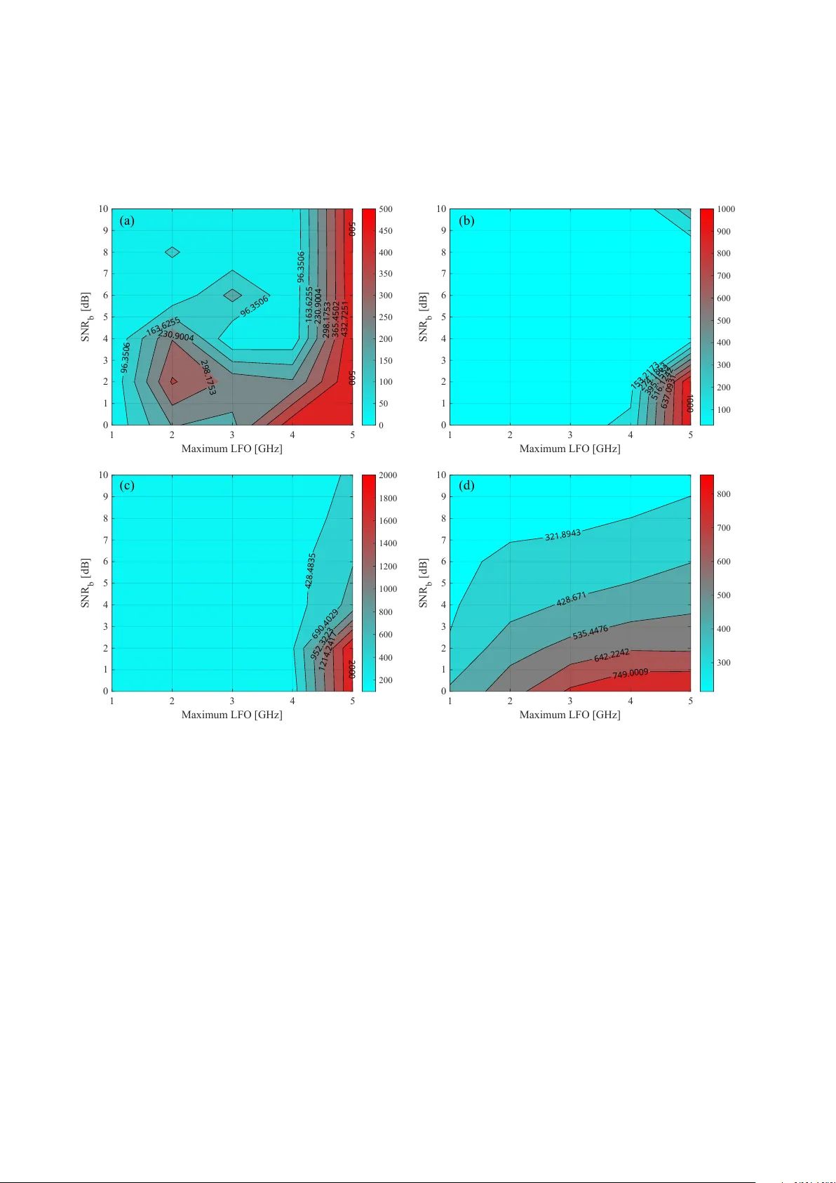
Sp ectral Segmen ted Linear Regression for Coarse Carrier F requency Oset Estimation in Optical LEO Satellite Comm unications I. P . Vieira, G. V. Serra, R. A. Colares, D. A. A. Mello ∗ † Abstract Carrier frequency oset estimation (CFOE) is a critical stage in modern coherent optical comm unication systems. Although conv en tional all-digital tec hniques p erform reliably in t ypical b er-optic communication links, CF OE often b ecomes a ma jor b ottleneck in low-sym b ol-rate scenarios with large carrier CFOs (ap- proac hing the signal bandwidth) and severe additiv e noise levels. These conditions are particularly prev alen t in links b et w een optical ground stations (OGSs) and low Earth orbit (LEO) satellites, where Doppler-induced frequency shifts of several gigahertz and atmospheric attenuation signicantly degrade CFOE p erformance and can render traditional methods ineectiv e. In this paper, w e prop ose a robust non-data-aided (NDA) scheme designed for wide-range CFOE. Such a coarse CFOE (C-CFOE) algorithm partially comp ensates for the CF O, enabling the operation of a subsequent ne CFOE algorithm. By applying low-complexit y op erations to the sp ectrum of the received signal, we recast the frequency estimation task as a segmented linear regression (SLR) problem. Numerical simulations in stress-test scenarios in volving large CFOs, low SNR, and low symbol rates sho w that the proposed approach ac hieves goo d estimation accuracy and robust conv ergence. Exp erimen tal oine v alidation further conrms the practical feasibility of the metho d. 1 In tro duction Coheren t optical detection com bined with adv anced digital signal pro cessing (DSP) techniques has b ecome a core tec hnology of mo dern optical communications [1]. This paradigm leads to signicant impro vemen ts in sp ectral eciency and receiver sensitivity enabled by techniques such as multilev el mo dulation formats and all-digital comp ensation of transmission impairmen ts. These capabilities hav e steered the evolution of industry standards to ward ultra-high p er-w av elength data rates approaching the terabit scale in b er-optic comm unication systems [2]. In free-space optical (FSO) systems, exp erimen tal demonstrations hav e achiev ed data rates ranging from tens of gigabits per second (Gbps), using in tensity-modulation/direct-detection (IM/DD) techniques [3, 4], to on the order of 100 Gbps with coheren t detection, including long-reach links in volving satellite comm unications [5]. These data rates are exp ected to increase substan tially in the coming years, p oten tially reac hing the terabit-per-second regime and b eyond [6, 7]. As FSO systems progressively adopt DSP-based coherent receivers to enable higher capacities, accurate carrier synchronization b ecomes a k ey p erformance-limiting factor. Links established b et ween optical ground stations (OGSs) and low-Earth-orbit (LEO) satellites represent some of the most challenging op erating scenarios, owing to a com bination of sev ere physical-la yer impairments and stringen t system constraints. The architecture of present-da y ultra-dense LEO constellations [8], with satellites tra veling at a t ypical orbital v elo cit y of 7.8 km p er second [9], can giv e rise to Doppler-induced frequency osets on the order of 4 GHz at a wa velength of 1550 nm [10]. Moreov er, the absence of in-line optical amplication, to- gether with propagation impairments suc h as scattering, absorption, and atmospheric turbulence, forces op eration under degraded signal-to-noise ratio (SNR) conditions. In practice, maintaining connectivity in distance-adaptive links ma y require reducing the symbol rate, whic h further increases phase noise-related impairments [11]. These factors collectively challenge conv en tional CFO estimation (CF OE) techniques dev elop ed for b er-based systems, motiv ating the need for robust, wide-range, and low-complexit y synchronization algorithms tailored to coherent optical LEO satellite communications. In this paper, we propose a no v el non-data-aided (ND A) CFOE algorithm based on segmen ted linear regression (SLR) applied to the cumulativ e p ow er sp ectral densit y (PSD) of the received signal. The algorithm op erates as a coarse CFOE (C-CFOE) stage that partially estimates and comp ensates the CFO, enabling the op eration of subsequen t ne CFOE (F-CFOE) algorithms applied on the residual CFO. The rationale behind the metho d is that, ideally , the cumulativ e PSD of a Nyquist-shap ed signal detected with excessive receiv er bandwidth is the concatenation of three straight segments, tw o of them ha ving the same slop e (corresp onding to the righ t and left noise o ors), and one of them having a steep er slop e (corresp onding to the signal p ortion of the sp ectrum). ∗ IPV, GVS, RAC, and D AAM are with the Department of Comm unications (DECOM), School of Electrical and Computer Engi- neering, Univ ersity of Campinas (UNICAMP), Campinas, SP , 13083-852, BR (email: darli@unicamp.br). † This work w as supp orted b y the Conselho Nacional de Desenvolvimento Cientíco e T e cnoló gic o (CNPq) and by the F ap esp Altave Multiuser Equipment Pr oje ct #2022/11596-0. 1 Suc h excessive receiver bandwidth is exp ected in distance-adaptive satellite links, where symbol rates are reduced to supp ort sustained connectivity under adverse attenuation conditions. The method is v alidated by sim ulation and lab oratory exp eriments under stringent requirements of near-zero SNR, low symbol rates, and high frequency osets, as often encountered in LEO satellite connections under challenging atmospheric and Doppler-shift condi- tions. The remainder of this pap er is organized as follows. Section 2 compiles related w orks. Section 3 introduces the prop osed metho d, detailing its theoretical foundations and implementation. Section 4 presents the simulation and exp erimen tal results. Finally , Section 5 concludes the pap er. 2 Related W orks Data-aided (DA) wide-range CFOE approaches hav e b een in vestigated as a means to ov ercome the limited es- timation range of con ven tional blind methods. Zhou et al. [12] prop osed a training-sequence-based wide-range CF OE algorithm that remov es the mo dulated phase information b y exploiting known training sym b ols, rather than relying on the traditional M -th pow er op eration. By decoupling the frequency estimation pro cess from the mo dulation format, the metho d achiev es an estimation range approaching half of the symbol rate, ± R s / 2 , in- dep enden tly of the mo dulation order, and demonstrates estimation errors on the order of a few megahertz for frequency osets of sev eral gigahertz in simulated 28-GBaud QPSK, 8-PSK, and 16-QAM systems. Similarly , Zhao et al. [13] introduced a digital pilot-aided CFOE technique in which a sp ecially designed pilot sequence gen- erates a pilot-tone-like sp ectral comp onen t, whose frequency shift can b e track ed in the frequency domain. Owing to this sp ectral structure, the metho d achiev es a wide estimation range theoretically b ounded by the receiver sampling rate and exhibits high estimation accuracy , with sub-megahertz v ariance under mo derate optical SNR (OSNR) conditions. In addition, the approach is shown to be largely insensitiv e to residual chromatic disp ersion and p olarization-mode disp ersion, and to op erate indep enden tly of the mo dulation format. More recently , He et al. [14] prop osed an almost-blind wide-range CFOE framew ork in the context of discrete-sp ectrum nonlinear frequency-division multiplexing (DS-NFDM) systems. By combining an eigenv alue-shift-based coarse estimation stage with a rened phase-error minimization criterion, the metho d achiev es wide CF O estimation ranges without baud-rate constraints, while requiring only t wo training sym b ols to resolve p eriodic am biguities. Exp erimen tal results demonstrate accurate CFO estimation for osets on the order of several hundreds of megahertz, with rep orted training-symbol ov erhead reductions exceeding 94-99% compared to fully training-assisted approaches. Despite their eectiv eness, the aforemen tioned tec hniques rely on em b edded pilot symbols or training sequences, in tro ducing nonzero ov erhead that may b e undesirable under stringent sp ectral-eciency constrain ts or non-static c hannels. In addition, their D A nature can limit robustness under severe noise conditions, where reliable pilot extraction and synchronization b ecome c hallenging. It is also worth noting that these wide-range CFOE metho ds w ere primarily dev elop ed and v alidated for b er-optic coheren t transmission systems, and their applicabilit y to optical satellite applications has not been explicitly addressed. In the context of optical satellite communications (OSC), Doppler-induced frequency osets ha ve b een ad- dressed at the system-design level. Almonacil et al. [15] prop osed a digital Doppler pre-comp ensation technique based on transmitter-side digital frequency shifting enabled by ephemeris-aided Doppler prediction. The approach exp erimen tally demonstrated comp ensation of frequency osets up to ± 10 GHz at line rates as high as 500 Gbps, with less than 0.7 dB additional optical launch p o wer p enalt y . While highly eective in mitigating large Doppler shifts (DSs), this strategy relies on accurate orbital information and transmitter-side adaptation, and does not directly address wide-range, blind CF OE at the receiver. More recently , F ernandes et al. [10] in tro duced a fully digital DS mitigation framework for coheren t LEO-to-Earth FSO links based on dynamic symbol-rate adaptation com bined with probabilistic constellation shaping (PCS). By jointly adapting the sym b ol rate and constellation en tropy , the metho d signicantly extends the tolerable CF O range, exp erimen tally supp orting osets exceeding ± 15 GHz in a 600 Gbps transmission. Nevertheless, this approac h op erates through transmitter-side parameter adaptation and assumes prior knowledge of the Doppler evolution, rather than p erforming ND A-CFOE at the receiv er. In practical coheren t receiv ers, state-of-the-art carrier frequency reco very (CFR) architectures commonly adopt a tw o-stage structure when dealing with large CFOs. A coarse CFO reco very (C-CF OR) stage is rst employ ed to estimate and comp ensate large frequency osets with relaxed accuracy requirements. This is follow ed by a ne CFO recov ery (F-CFOR) stage, which renes the residual oset using high-accuracy techniques such as M -th p o w er estimators or pilot-aided methods. The presence of a reliable C-CFOR stage is critical, as it ensures that the residual frequency oset falls within the narrow acquisition range of ne estimators. In [16], we presen t a tw o-stage comp ensation strategy combining a coarse CFOE (C-CF OE) metho d derived from [17] with a subsequent M -th p o w er-based ne correction, targeting DS mitigation in optical inter-satellite links (OISLs) under architectures represen tative of recent commercial LEO constellations. The C-CFOE stage, originally prop osed by Diniz et al. [17], is based on an im balance b et ween the positive ( P + ) and negativ e ( P − ) sp ectral components of the receiv ed signal, where the CF O is estimated as b eing prop ortional to the logarithm of the ratio P + /P − . Lately , Chino et al. [18] prop osed an interesting tw o-stage CFO estimation method for inv erse scattering transform (IST)- based transmission systems, where eigenv alue shifts enable wide-range acquisition and the scattering co ecien t 2 b is exploited for ne estimation. While the approach achiev es wide estimation range and high accuracy , it is inheren tly tied to nonlinear F ourier transform (NFT)/IST signal representations and cannot b e directly applied to conv en tional linear coherent mo dulation formats. Sev eral other blind CFO estimation metho ds hav e b een prop osed for sp ectrally ecient transmission archi- tectures, such as digital sub carrier m ultiplexing (DSM) and discrete-sp ectrum modulation [19, 20, 21, 22, 23]. These metho ds typically exploit sp ectral features, such as sp ectral edges, dips, or p o wer im balance, to infer the frequency oset without explicit training symbols. Overall, existing CFO estimation techniques face a trade-o b et w een estimation range, accuracy , computational complexit y , and reliance on training o verhead. In particular, the problem of wide-range-NDA CFOE under low symbol-rate and lo w-SNR conditions remains insuciently ad- dressed, motiv ating the dev elopment of alternativ e approaches that combine wide acquisition range with robust con vergence and low implementation complexity . 3 Metho dology 3.1 Principle of Op eration The prop osed CFOE algorithm takes the p eriodogram of the ov ersampled received signal as a starting p oin t. The sampling frequency , F s , must b e such that it allows the maximum exp ected frequency oset, ∆ f max , to b e adequately accommodated in the receiv er bandwidth. This is a reasonable assumption in distance-adaptive satellite links, where the sym b ol rate can b e strongly reduced to operate at stringent atten uation conditions. Next, the signal’s perio dogram p o w er spectral densit y (PSD) is cum ulated o ver frequency throughout the entire reception band. F or a discrete-time signal y [ n ] , n = 0 , 1 , · · · , N − 1 , with DC-centered discrete F ourier transform (DFT) Y [ k ] =  P N − 1 n =0 y [ n ] e − j 2 π ( k − N/ 2) n/ N  , k = 0 , 1 , · · · , N − 1 , the cumulativ e bandlimited pow er reads: P acc ( f m ) = 1 N m : f k ≤ f m X k =0 | Y [ k ] | 2 δ f , f m ∈ [ − F s / 2 , F s / 2) , (1) where δ f = F s / N is the frequency resolution and f k = ( k − N/ 2) δ f is the frequency v alue at the k -th bin. Figure 1a depicts the PSD of a 2-GBd p olarization-m ultiplexed (PM)-QPSK signal impaired b y a frequency oset of ∆ f = 3 . 5 GHz, computed using a 1024-symbol FFT blo c k. Applying cum ulativ e in tegration to the PSD yields the c haracteristic prole shown in Fig. 1b. Line segmen ts I and I II correspond to the result of the integration pro cess in the noise o or region, th us ha ving slopes that are close to each other and lo w er than those of segmen t I I, referring to the region of the sp ectrum that con tains the signal. In this sense, the pro jection of segmen t I I on to the f -axis represents the signal’s bandwidth. Accordingly , in baseband, the distance from its midp oin t to the origin yields an estimate of the frequency oset to which the signal is sub jected. 3.2 Segmen ted linear regression (SLR) In this pap er, we prop ose the use of SLR techniques to estimate the CFO of the received signal, shaping and discriminating regions I, II and I I I in the spectral domain. SLR mo dels assume that the conditional mean function of a resp onse v ariable y given a predictor x , E [ y | x ] , is piecewise linear, showing distinct linear relationships ov er sp ecic interv als of the co v ariate space. F ormally , let Ψ = { ψ 1 < ψ 2 < · · · < ψ K } be an ordered set of structural c hange p oints, referred to as breakp oints, that partition the domain of x into K + 1 contiguous segmen ts such that E [ y | x ] =            β 0 , 1 + β 1 , 1 x, x < ψ 1 , β 0 , 2 + β 1 , 2 x, ψ 1 ≤ x < ψ 2 , . . . β 0 ,K +1 + β 1 ,K +1 x, x ≥ ψ K , (2) where B = { ( β 0 ,j , β 1 ,j ) } K +1 j =1 denotes the collection of regime-sp ecic intercept and slop e parameters. In general, b oth the regression parameters and the breakp oin ts are unknown and must b e estimated from the data, most often by minimizing a least-squares criterion. Under the con tin uity constraint, β 0 ,j + β 1 ,j ψ j = β 0 ,j +1 + β 1 ,j +1 ψ j , ∀ j = 1 , · · · , K , the conditional mean function E [ y | x ] is allow ed to c hange slop e but not level, and the mo del simplies to the canonical compact parametric represen tation [24] y i = β 0 + β 1 x i + K X k =1 φ k ( x i − ψ k ) + + ε i , ψ 1 < ψ 2 < · · · < ψ K , (3) where β 0 ( β 1 ) is the baseline intercept (slop e) – i.e., that applying for x < ψ 1 –, φ k corresp onds to the incremental slop e con tribution after the k -th breakp oin t, ( · ) + = max { 0 , ·} is the hinge function, and ε i is a random error term satisfying E [ ε i | x i ] = 0 and V ar ( ε | x i ) = σ 2 < ∞ . 3 0 0.1 0.2 0.3 0.4 0.5 0.6 0.7 0.8 0.9 1 -8 -6 -4 -2 0 2 4 6 8 Frequency [GHz] 0 0.1 0.2 0.3 0.4 0.5 0.6 0.7 0.8 0.9 1 Normalized Cumulative PSD 0 Hz -5 GHz -2.5 GHz 2.5 GHz 5 GHz -15 -10 -5 0 5 10 15 Frequency [GHz] 0 0.1 0.2 0.3 0.4 0.5 0.6 0.7 0.8 0.9 1 Normalized Cumulative PSD 8 GBd 4 GBd 2 GBd 1 GBd -8 -6 -4 -2 0 2 4 6 8 Fre quency [GHz] 0 0.1 0.2 0.3 0.4 0.5 0.6 0.7 0.8 0.9 1 Normalized Cumulative PSD 0 dB 5 dB 10 dB 15 dB 20 dB -8 -6 -4 -2 0 2 4 6 8 Fr equency [GHz] -30 -25 -20 -15 -10 -5 0 Amplitude [dB] Figure 1: (a) Sp ectrum of a 2-GBd PM-QPSK signal, shaped by a ro ot-raised-cosine (RRC) lter with roll-o factor α = 0 . 1 , at 1-dB SNR p er bit and impaired b y a 3.5-GHz CFO and its (b) corresp onding normalized cumulativ e linear PSD – with SNR, signal bandwidth ( R s (1 + α ) ), and CFO ( ∆ f ) indicated –, forming a characteristic three- segmen t piecewise-linear structure. Impact of dierent (c) p er bit SNR levels, (d) sym b ol rates, and (e) CF Os in the cumulativ e PSD b eha vior. The accum ulation process suppresses high-frequency uctuations, yielding a more pronounced contrast across the noise-oor and signal-region regimes under SNR v ariation. The successful SLR application dep ends on three basic assumptions [25]: (i) the num b er of regimes is small relativ e to the sample size; (ii) within each regime, the conditional exp ectation is w ell approximated by linear functions; (iii) transitions b et ween adjacen t regimes are abrupt – manifested as changes in slop e – rather than gradual. Figures 1c-e show the result of the PSD accumulation pro cess ov er an 1024-FFT blo c k for dierent SNR lev els, symbol rates, and CF Os, resp ectiv ely . Because of the pattern formed in the received band, SLR assumptions (i) and (ii) are alwa ys true. Assumption (iii), in its turn, tends to b ecome less robust as the SNR decreases: low er SNR tends to smo oth out abrupt regime b oundaries. Nev ertheless, a clear violation arises only in the limiting case where the SNR approaches zero. 3.3 Algorithm This section presents the general concepts underlying the spectral SLR-based C-CF OE. Figure 2 shows the complete ow diagram of the prop osed C-CFOE metho d, which is applied to each FFT block, including all pro cessing stages leading to the frequency oset estimation. As can b e seen, b oth b efore and after the application of the SLR method, some pro cessing steps are required to ensure the quality of the estimation. In what follows, w e conduct a walkthrough of the diagram blo c ks, discussing their roles in the metho dology . 3.3.1 Data Prepro cessing and Numerical Conditioning Before the CFOE can b e eectively p erformed through SLR algorithm, a set of prepro cessing steps m ust b e carried out to ensure reliable op eration and n umerical stability . The DSP o w b egins by splitting the received signal, initially in the time domain, into xed-size blocks and computing their corresp onding frequency-domain represen tations using the DFT. Subsequently , the PSD of each blo c k is calculated for b oth polarizations. Since the frequency oset aecting eac h polarization is approximately the same, the tw o PSDs are com bined, con tributing to the reduction of the relative noise p o wer. At this stage, a forgetting factor ξ FFT is applied to suppress high- frequency noise uctuations, resulting in more stable FFT estimates. F ollowing this, a downsampling step is p erformed to remov e surplus samples pro duced by the analog-to-digital conv erter (ADC). The excess sampling requiremen t arises from t w o main factors. First, the receiv er m ust accommo date the maxim um exp ected frequency oset, ∆ f max , to which the signal may b e sub jected. Second, due to the w ay the method is constructed, a minim um 4 sp ectral margin must b e ensured to properly dene the three op erating regimes – where the signal region is eectiv ely conned b et w een the noise o ors. Accordingly , the downsampling factor is expressed as N ↓ = 2 $ log 2 F s 2 max { R s (1+ α ) 2 +∆ f max , R s } !% , (4) where ⌊·⌋ denotes the o or op erator, max {· , ·} returns the maximum of its tw o argumen ts, and α is the roll-o factor of the pulse-shaping lter. The next step inv olves integrating the ltered PSD across the en tire reception band, as described in Eq. (1). Due to the nite observ ation window and pulse shaping transients at the blo c k b oundaries, FFT bins located near the edges of the occupied spectrum typically exhibit reduced and distorted sp ectral con tent, particularly at low sym b ol rates, as shown in Fig. 3. T o mitigate this eect and ensure reliable CFOE, frequency bins corresp onding to the spectral boundaries are excluded from the estimation process. F ollowing the diagram o w, the next stage corresp onds to axis normalization: the accum ulated PSD is scaled suc h that its maxim um v alue equals unity , and the frequency axis ranges [ − 0 . 5 , 0 . 5] . At this p oint, the samples are ready to pro ceed to the SLR algorithm, where the tw o breakpoints, ψ 1 and ψ 2 , are estimated. It follo ws that the a verage of the breakp oin ts m ultiplied b y the normalization scale factor results in the estimation of the blo ck frequency oset, c ∆ f . Finally , to enhance the stabilit y of the estimation, a new forgetting factor, ξ c ∆ f , is in tro duced within c ∆ f , implementing a low-pass ltering op eration. 3.3.2 Breakp oin t and Slop e Estimation W e no w summarize the closed-form, implementation-ready procedure used to estimate the tw o breakp oin ts, ψ 1 and ψ 2 , as well as the corresponding slopes of a con tinuous three-segment piecewise-linear mo del, following the approac h originally prop osed by Jacquelin [26]. The deriv ation of the formulas employ ed here is provided in App endix A. Let { ( x i , y i ) } N i =1 b e the input data, where x i denotes the indep enden t v ariable and y i is the resp onse, with strictly increasing abscissae, x 1 < · · · < x N . The goal is to t a con tinuous piecewise-linear function with slop es p ≡ ( p 1 , p 2 , p 3 ) T , separated by tw o unkno wn breakp oin ts ψ 1 < ψ 2 , and intercepts q ≡ ( q 1 , q 2 , q 3 ) T for each segmen t. The estimation pro ceeds in t wo stages: rst, an auxiliary regression is used to estimate ψ 1 , ψ 2 (steps 1 to 4); second, a standard linear regression is used to estimate the slop es and in tercepts (steps 5 and 6). Step 1 (Discrete primitiv es). Dene S y [ i ] and S xy [ i ] as discrete numerical primitiv es of the sampled quantities y and xy , respectively , computed b y the trap ezoidal rule: S y [1] = 0 , S y [ i ] = S y [ i − 1] + y i − 1 + y i 2 ( x i − x i − 1 ) , S xy [1] = 0 , S xy [ i ] = S xy [ i − 1] + x i − 1 y i − 1 + x i y i 2 ( x i − x i − 1 ) , i = 2 , . . . , N . Th us, S y [ i ] ≈ R x i x 1 y ( x ) dx and S xy [ i ] ≈ R x i x 1 xy ( x ) dx . Step 2 (Construction of breakp oin t regressors). Using the quan tities ab o ve, construct the auxiliary regres- sors. F or eac h i = 1 , . . . , N , dene F 0 ,i = y i , F 1 ,i = 6 S xy [ i ] − 2 x i S y [ i ] − x 2 i y i , F 2 ,i = x i y i − 2 S y [ i ] , F 3 ,i = x i , F 4 ,i = 1 . Figure 2: Schematic of the C-CF OE metho d. 5 -8 -6 -4 -2 0 2 4 6 8 Frequency [GHz] 0 20 40 60 80 100 120 140 160 180 Cumulative PSD -5.14 GHz -5 GHz Boundary distortion 6.5 7 7.5 8 Frequency [GHz] 140 145 150 155 160 165 170 Cumulative PSD Figure 3: Impact of FFT b oundary-bin exclusion on frequency-estimation accuracy , emphasizing distortions intro- duced b y pulse shaping and nite observ ation windows. Sp ectral-edge artifacts arise when the PSD is accum ulated for a RRC-shaped 1-GBd PM-QPSK signal (span: 20 sym b ols, roll-o factor α = 0 . 1 ), at 64 samples p er symbol and impaired b y a -5 GHz CF O. The blue and red squares mark the breakp oin ts ψ 1 and ψ 2 , resp ectiv ely , ob- tained from the full PSD and frequency vectors, whereas the circles indicate the estimates after excluding edge samples. F or the considered FFT blo c k, using the complete cumulativ e PSD and frequency vectors results in a CF O o verestimation of approximately -140 MHz (green square). In contrast, removing b oundary bins mitigates edge distortions and yields an accurate CFO estimate, as indicated b y the green circle. Here, F i ≡ ( F 1 ,i , F 2 ,i , F 3 ,i , F 4 ,i ) T denotes the predictor vector of an auxiliary linear regression whose co ecien ts are used to compute the breakpoint lo cations. Step 3 (Estimation of auxiliary co ecients). F orm the normal equation matrix, M F , and the corresp onding righ t-hand-side v ector, b F , of this regression as M F = N X i =1 F i F T i , b F = N X i =1 F 0 ,i F i . The co ecien t v ector C ≡ ( C 1 , C 2 , C 3 , C 4 ) T is then obtained by solving the linear system C = M − 1 F b F . Step 4 (Closed-form breakpoint estimation). The breakp oin ts are giv en as the tw o ro ots of a quadratic expression inv olving C 1 and C 2 : ψ 1 , 2 = C 2 ∓ p C 2 2 − 4 C 1 2 C 1 , ψ 1 < ψ 2 . Step 5 (Construction of slop e regressors). Giv en ψ 1 and ψ 2 , w e construct regressors that represen t a con tinuous piecewise-linear function with three segmen ts. Let H ( t ) = 1 t ≥ 0 b e the Heaviside function. F or eac h i = 1 , · · · , N , dene G 1 ,i = x i − ( x i − ψ 1 ) H ( x i − ψ 1 ) , G 2 ,i = ( x i − ψ 1 ) H ( x i − ψ 1 ) − ( x i − ψ 2 ) H ( x i − ψ 2 ) , G 3 ,i = ( x i − ψ 2 ) H ( x i − ψ 2 ) , G 4 ,i = 1 . These regressors G i ≡ ( G 1 ,i , G 2 ,i , G 3 ,i , G 4 ,i ) T dene the con tributions of the rst, second, and third linear segments o ver the in terv als x < ψ 1 , ψ 1 ≤ x < ψ 2 , and x ≥ ψ 2 , respectively , while preserving contin uity of the tted function. Step 6 (Estimation of slop es). F orm the normal equation matrix, M G , and right-hand-side vector, b G , of this regression as M G = N X i =1 G i G T i , b G = N X i =1 y i G i , 6 and solve ( p 1 , p 2 , p 3 , q 1 ) T = M − 1 G b G . Here, p 1 , p 2 , and p 3 determine the segmen t gradien ts, while q 1 corresp onds to the intercept of the rst line segmen t. The contin uit y at ψ 1 and ψ 2 uniquely determines the remaining intercepts q 2 and q 3 as q 2 = q 1 + ( p 1 − p 2 ) ψ 1 , q 3 = q 2 + ( p 2 − p 3 ) ψ 2 . The o verall pro cedure requires computing tw o cumulativ e sums and the solution of tw o linear systems of size 4 × 4 , with no nonlinear optimization or iterativ e search. F urthermore, it is worth noting that, for the CFO estimation purp oses, simply obtaining the breakp oin ts in step 4 is sucient. Figure 4 illustrates the application of the metho d to a dual-polarization QPSK transmission at a sym b ol rate of 1 GBd, under a frequency oset three times larger than the symbol rate. The estimation corresp onds to the nal FFT blo c k of the signal, after b oth the FFT pro cessing and the estimator hav e fully stabilized under the inuence of the forgetting factors ξ FFT and ξ c ∆ f . Normalization of the x - and y -axes impro ves numerical stability . T wo breakp oin ts, ψ 1 = (0 . 16 , 0 . 5) and ψ 2 = (0 . 22 , 0 . 8) , are iden tied, along with the slop es of the three corresp onding line segments. -0.5 0 0.5 x 0 0.1 0.2 0.3 0.4 0.5 0.6 0.7 0.8 0.9 1 y Segment 1: y = 0.77221x + 0.37488 Segment 2: y = 4.1226x - 0.12695 Segment 3: y = 0.74887x + 0.63336 2 (0.22, 0.8) 1 (0.16, 0.5) Figure 4: SLR-based estimation applied to a 1-GBd QPSK signal aected by a 3-GHz CFO. Both axes are normalized to enhance numerical stability . 3.4 Complexit y The SLR pro cedure for breakp oint estimation requires ∼ 60 N elemen tary arithmetic op erations, where N denotes the n umber of data samples, as summarized in T ab. 1. Consequently , the total o verall computational complexit y of the procedure follows O ( N ) . F rom a hardw are implemen tation p erspective, the Jacquelin metho d is w ell-suited for real-time signal pro cessing owing to its non-iterative structure and linear computational complexity . The algorithm follo ws a xed sequence of elementary arithmetic op erations without requiring iterativ e renement, matrix fac- torizations, or transcendental function ev aluations. This deterministic execution o w ensures predictable latency and b ounded computational cost, which are critical for deploymen t in high-throughput, low-latency optical signal pro cessing systems. F urthermore, the streaming data access pattern requires only constant memory and enables straigh tforward pip elining, making the metho d particularly amenable to ecient xed-p oint implementations on em b edded pro cessors. Bey ond Jacquelin’s formulation of SLR, alternative strategies can also b e considered. In particular, metho ds based on iterative renement and likelihoo d-based criteria – suc h as those implemented in the se gmente d [27] and pie c ewise-r e gr ession [28] pac kages – pro vide a more exible formulation for breakp oint estimation. These metho ds require initial guesses for the breakp oin t lo cations, whic h are subsequently rened through an iterative optimization pro cedure (e.g., via score-based or Newton-type up dates), allowing for the joint estimation of b oth regression parameters and breakp oint locations. As iterative pro cedures, how ev er, they may b e sensitiv e to initialization and are not guaranteed to con verge in all cases; moreov er, they are generally more computationally demanding than the closed-form approach considered here. F or this reason, suc h strategies are not pursued in this w ork, as the fo cus is on low-complexit y implementations with predictable computational cost. 7 T able 1: Num ber of elementary arithmetic op erations (additions/subtractions, multiplications, and divisions) required at each step of the Jacquelin SLR algorithm. The op eration counts assume that the inv erses of the 4 × 4 matrices inv olved in the normal equations are precomputed, so that solving the linear systems reduces to a matrix-v ector m ultiplication. Step A dd/Sub Mult Div Remark 1 5 ( N − 1) 7 ( N − 1) 0 T rap ezoidal-rule accumulation of S y and S xy 2 3 N 7 N 0 Construction of F i 3 4 (5 N + 2) 4 (5 N + 4) 0 F ormation of M F , b F , and matrix-v ector pro duct 4 3 3 2 ψ 1 and ψ 2 ; one square-ro ot ev aluation 5 6 N 4 N 0 Construction of G i 6 4 (5 N + 2) +6 4 (5 N + 4) 0 F ormation of M G , b G , and matrix-v ector pro duct T able 2: Simulation Scenarios. Scenario Description ( f mean ) max (GHz) SNR (dB) R s (GBd) (a) Large CF O 10 15 32 (b) Lo w SNR 5 0 32 (c) Lo w Sym b ol Rate 1 15 4 4 Results and Discussion This section ev aluates the performance of the proposed SLR-based CF OE strategy under operating conditions rep- resen tative of optical satellite communications, assuming a dual-p olarization QPSK transmission system through- out the analysis. Numerical simulations are rst used to assess estimation range, accuracy , and conv ergence b e- ha vior in the presence of large CF Os, low SNRs, and reduced sym b ol rates (corresponding to increased phase-noise impact). The robustness of the prop osed approach is further examined through oine exp erimen tal v alidation, based on long-duration signal captures, demonstrating frequency-drift tracking capabilit y and characterizing the residual frequency osets obtained from real measuremen t data. The results presented here are obtained using Jacquelin’s integral-equation-based linearization approach for segmented linear regression [26]. F urther metho d- ological details are given in Appendix A. 4.1 Numerical Sim ulations In practical optical systems, transmitter and LO lasers are sub ject to systematic frequency deviations as well as time-v arying uctuations resulting from imp erfect calibration, thermal drift, environmen tal p erturbations, and in trinsic phase noise. Accordingly , the instan taneous carrier frequency deviation is typically mo deled with a sin usoidal prole ∆ f ( t ) = f mean + f pk - pk 2 sin(2 π f j t ) , (5) where f mean is the mean CFO, f pk - pk denotes the p eak-to-peak frequency excursion, f j is the frequency of the imp osed temp oral v ariation, and t is the time. The OIF-800ZR standard [2] sp ecies four distinct frequency tones ∆ f ( t ) . These tones, illustrated in Fig. 5, dene the parameters f pk - pk (v ertical axis) and f j (horizon tal axis) in Eq. (5). In the rst simulation round, w e apply these four tones in three extreme op erating conditions (scenarios (a) to (c)) representativ e of optical satellite links, whic h are independently assessed by v arying one stress condition at a time. The numerical v alues implemen ted in the four scenarios are presented in T able 2. Scenario (a) corresp onds to a large f mean , as typ- ically encountered in LEO-LEO inter-satellite links [29]. Scenario (b) addresses lo w signal-to-noise ratio (SNR) conditions, whic h are characteristic of links trav ersing the Earth’s atmosphere, such as LEO-OGS or OGS-LEO links [30, 31]. Finally , scenario (c) considers an operation at a low symbol rate, whic h can occur in the context of distance-adaptiv e transmission [32, 33]. T able 3 presents the estimation error results for the combination of three scenarios and four ∆ f ( t ) tones. Eac h entry rep orts the worst estimation error p er block relative to the applied reference CF O, i.e., max | ∆ f [ k ] − c ∆ f ∗ [ k ] | for the k -th blo c k, ev aluated o ver 50 independent channel realizations. F or eac h conguration, the mean CF O parameter f mean in Eq. (5) is randomly drawn from a uniform distribution whose supp ort is b ounded by the maximum absolute v alue of the mean CFO, denoted by ( f mean ) max , such that | f mean | ≤ ( f mean ) max 1 . The random v alues are generated using a Mersenne T wister pseudo-random n umber generator initialized with seed 0. When the proposed estimator is employ ed as a rst-stage CF O recov ery (i.e., a C-CFOR), the resulting residual 1 F or instance, when ( f mean ) max = 10 GHz, the realizations are generated with f mean ∼ U ([ − 10 GHz , 10 GHz]) . In the algorithm, while f mean spans multiple v alues within this in terv al across realizations, the maximum exp ected CFO is kept xed as ∆ f max = ( f mean ) max + f pk - pk / 2 . 8 10 2 10 4 10 6 10 8 10 10 Drift frequency [Hz] 10 0 10 1 10 2 Peak-to-peak frequency [MHz] T 1 T 2 T 3 T 4 Figure 5: Combinations of f pk - pk (y-axis) and f j (x-axis) that pro duce four dierent tones (T 1 –T 4 ), following the description in [2]. T able 3: Maximum CFO estimation error ev aluated across 50 realizations under three stress-case conditions: (a) Large CFO ( ∆ f = 10 GHz, SNR = 15 dB, R s = 32 GBd); (b) Low SNR ( ∆ f = 5 GHz, SNR = 0 dB, R s = 32 GBd); and (c) Low symbol rate ( ∆ f = 1 GHz, SNR = 15 dB, R s = 4 GBd). In each case, the rst 100 FFT blo c k w ere discarded to account for algorithm con vergence. Scenario T one 1 (T 1 ) T one 2 (T 2 ) T one 3 (T 3 ) T one 4 (T 4 ) (a) 521.25 MHz 521.05 MHz 449.13 MHz 763.82 MHz (b) 1.69 GHz 1.69 GHz 1.68 GHz 1.69 GHz (c) 57.04 MHz 56.26 MHz 57.72 MHz 57.67 MHz frequency osets consistently lie within the correction range of the 4th-pow er algorithm ( R s / 8 ), thereby enabling accurate ne CFO comp ensation in a subsequent stage. Moreov er, the residual frequency estimates remain largely consisten t across the dieren t applied tones, indicating that the estimator p erformance is only weakly dep enden t on the sp ecic tone characteristics. In the large-oset regime (scenario a), the CFO is reduced from 10 GHz to sub-gigahertz residuals, with w orst-case v alues b elo w 800 MHz. Although some disp ersion is observ ed across tones – most notably for T 4 – the residual osets remain more than a factor of four b elo w the upper correction limit of the 4th-pow er algorithm. Under low-SNR op eration (scenario b), the estimator exhibits remarkably stable b eha vior, yielding nearly iden tical residual osets across all tones. Despite the elev ated noise lev el, which increases conv ergence time, the residual CFO remains around 1.7 GHz, demonstrating that estimator p erformance is largely insensitive to tone-dep enden t dynamics in noise-dominated regimes. Finally , in the low-sym b ol-rate case (scenario c), corresp onding to increased phase-noise impact, the estimator achiev es residual osets on the order of 60 MHz – more than an order of magnitude reduction relative to the initial oset and well b elow the F-CF OE threshold. The narro w spread across tones further indicates stable b eha vior across the dierent tones even when the symbol rate is reduced to one quarter of the CF O. T aken together, these results indicate that, for the scenarios considered, the prop osed estimator deliv ers consis- ten t and predictable residual CF O lev els across a wide range of op erating conditions, with only w eak dep endence on the sp ecic tone c haracteristics. Next, this analysis is extended to more stringent conditions in which these impairmen ts are jointly applied, allo wing the estimator p erformance to b e assessed under comp ounded stress. Figure 6 presen ts the maximum estimation error of the coarse frequency estimator for four symbol rates – namely 4, 8, 16, and 32 GBd – while jointly v arying the bit-wise SNR (SNR b ) b et w een 0 and 10 dB and the maxim um v alue for the frequency oset, ∆ f ( t ) , b et ween 1 and 5 GHz. In our implementation, the receiv er operates at a xed sampling rate of F s = 64 GSa / s , spanning R s = 2 n GBd ( 2 ≤ n ≤ 5 ). F or the CFO, w e consider the same sinusoidal prole in Eq. (5), with f mean ∈ U ( − ∆ f max , ∆ f max ) , f pk - pk = 200 MHz, and f j = 100 kHz. As exp ected, the most challenging operating regime across all cases corresp onds to the simultaneous presence of large CF Os and low SNR b , where noise-induced estimation uncertaint y and reduced observ ation quality – stemming from the nite resolution of the FFT – hinder reliable CF O estimation. Despite this comp ounded impairment, the estimator exhibits robust p erformance ov er a broad region of the parameter space. In particular, for ∆ f < 4 GHz and SNR b > 1 dB, the coarse CFO estimator (C-CFOE) consisten tly reduces the residual frequency oset to 9 within the capture range required by the subsequen t 4th-p o wer algorithm. This b eha vior is observed across all ev aluated symbol rates, indicating that the prop osed estimator maintains eective acquisition capabilit y even as the symbol rate decreases and the relative CF O b ecomes more severe, given that the 4th-p o wer algorithm exhibits a baud-rate-dep enden t capture range ( ∆ f = ± R s / 8 ). Ov erall, these results demonstrate that reliable coarse CF O correction can be achiev ed under stringen t op erating conditions relev an t to optical satellite communication systems, thereby pro viding a solid foundation for subsequent ne sync hronization stages. 96.3506 96.3506 96.3506 163.6255 163.6255 230.9004 230.9004 298.1753 298.1753 365.4502 432.7251 500 500 1 2 3 4 5 Maximum LFO [GHz] 0 1 2 3 4 5 6 7 8 9 10 SNR b [dB] 0 50 100 150 200 250 300 350 400 450 500 153.2173 274.1863 395.1552 516.1242 637.0931 1000 1 2 3 4 5 Maximum LFO [GHz] 0 1 2 3 4 5 6 7 8 9 10 SNR b [dB] 100 200 300 400 500 600 700 800 900 1000 428.4835 690.4029 952.3223 1214.2417 2000 1 2 3 4 5 Maximum LFO [GHz] 0 1 2 3 4 5 6 7 8 9 10 SNR b [dB] 200 400 600 800 1000 1200 1400 1600 1800 2000 321.8943 428.671 535.4476 642.2242 749.0009 1 2 3 4 5 Maximum LFO [GHz] 0 1 2 3 4 5 6 7 8 9 10 SNR b [dB] 300 400 500 600 700 800 (a) (b) (c) (d) Figure 6: The estimator p erformance is ev aluated under multiple op erating scenarios, considering 100 independent c hannel realizations and a total of 2 18 transmitted sym b ols. The maxim um estimation error is dened as the largest deviation from the reference frequency observed after 100 FFT blocks. Operating regimes combining SNR and lo w sym b ol rate with large frequency osets constitute the most c hallenging cases from a carrier synchronization p erspective. Using FFT s of 1024 samples in the estimator and setting ξ PSD = ξ c ∆ f = 0 . 98 , the prop osed method is able to pro duce a residual frequency oset smaller than R s / 8 , whic h is required by the 4th-p o wer algorithm for F-CF OE, across all ev aluated scenarios with ∆ f max ≲ 4 GHz , even at SNR b = 1 dB . In Fig. (a), corresp onding to R s = 4 GBd , the allo wable ∆ f max margin gradually increases with SNR. In Figs. (b) and (c), with R s = 8 GBd and R s = 16 GBd , resp ectiv ely , the estimator op erates reliably for ∆ f max ≤ 5 GHz ov er the entire region where SNR b > 2 . 5 dB . Finally , in Fig. (d), corresp onding to R s = 32 GBd , the estimator remains op erational o v er the full ev aluated region, maintaining a comfortable margin with respect to the maximum allow able residual frequency oset of 4 GHz . 4.2 Exp erimen tal V alidation Exp erimen tal measurements were carried out to ev aluate the C-CF OE p erformance using the setup depicted in Fig. 7. A t the transmitter, digital wa v eforms are generated oine and replay ed by an arbitrary wa veform generator (A WG, Keysight M8199A-A TO) op erating at 128 GSa/s. These wa veforms corresp ond to a 15th and 11th-order pseudo-random binary sequence (PRBS-15 and PRBS-11, resp ectively , to create dierent sequences in eac h channel) transmitted at a symbol rate of 4 GBaud. This relatively low symbol rate was selected to em ulate very stringen t frequency recov ery conditions where the frequency oset approaches or surpasses the signal 10 OS A CohRX 0.3 nm 10 90 3 dB Noise generator DP- IQ A WG DSO ASE ECL IDPhotonics OMFT -C-01-F A Keysight M8199A-A T O Keysight N4391B-059 Keysight UXR0594A Padtec LOAC21 1GAH Padtec LOAC21 1GAH Figure 7: Experimental setup for the ev aluation of the prop osed C-CFOE algorithm. A WG: arbitrary w av eform generator; DP-IQ: dual-p olarization in-phase/quadrature mo dulator; VO A: v ariable optical attenuator; EDF A: erbium-dop ed b er amplier; OBPF: optical bandpass lter; OMA: optical mo dulation analyzer; DSO: digital storage oscilloscop e. bandwidth. The resulting electrical signals drive a dual-p olarization in-phase/quadrature mo dulator (DP-IQ, IDPhotonics OMFT-C-01-F A), which mo dulates a narrow linewidth ( < 25 kHz) contin uous-wa ve optical carrier. An optical isolator is placed after mo dulation to suppress bac k-reections and preven t optical feedback. After mo dulation, the optical signal is amplied by an erbium-dop ed b er amplier (EDF A, P adtec LOA C211GAH) and mixed with amplied sp on taneous emission noise through a 3-dB coupler. The noise level is attenuated by a v ariable optical atten uator (VO A, Eigenlight 420 WDM) equipp ed with an integrated p o w er meter to con trol noise p o wer and consequently the SNR. The mixed signal and noise pass through a 37.5-GHz lter enabled by a wa velength selective switch (WSS) to ensure sp ectral consistency . This bandwidth is selected to ensure a at sp ectrum around the signal and preven t cutting sp ectral conten t needed for DSP . The resulting shap ed signal then passes through a 90:10 optical coupler: 90% of the p o wer is directed to the coherent receiver (CohRX), while the remaining 10% is sen t to an optical sp ectrum analyzer (OSA) with 0.1-nm resolution bandwidth for SNR measurement. Coherent detection is p erformed using a free-running lo cal oscillator (LO) laser within an optical mo dulation analyzer (OMA, Keysight N4391B-059). The electrical outputs of the coherent receiver are subsequen tly sampled at 32 GSa/s by a high-sp eed digital storage oscilloscope (DSO, Keysight UXR0594A) and pro cessed oine. Figure 8 shows the algorithm trac king ov er an aquisition time of ∼ 4 ms, at SNR b = 5 dB, corresp onding to 61,035 FFT blo cks of 1,024 samples each. The tw o curves indicate the unltered and ltered cases. The algorithm rev eals a systematic frequency oset of ab out 640 MHz b etw een the transmitter and the LO, along with p eak- to-p eak oscillations of about 150 MHz. As data acquisition w as carried out at 4-GBd symbol rate, the obtained p erformance would not b e achiev ed b y the traditional 4th-p o wer algorithm, which has an estimation b ound of R s / 8 , in this case, only 500 MHz. T o ev aluate the capability of C-CFOE to reduce the CFO b elo w the threshold required by the 4th-p o wer algorithm, a series of exp erimen tal measurements was p erformed for a 4-GBd PM-QPSK transmission (16 Gbps). The SNR p er bit w as ev aluated at three lev els: 0, 5, and 10 dB. In addition to the intrinsic frequency oset betw een the T x and LO lasers ( ∼ 640 MHz, as previously ev aluated), four additional scenarios were considered (-4 GHz, -2 GHz, 2 GHz, and 4 GHz), in whic h an inten tional CFO was applied to the T x laser. The data acquisition time for these ev aluations was 500 µ s. Figure 9 shows the PSD accumulation proles for the last pro cessed blo c ks in each case considered. It can b e observed that in the scenario where no external CFO is applied (dashed black curves), the midp oin t of the cen tral segmen t, referring to the signal, is slightly shifted to the right, in accordance with the systematic CFO sho wn in Fig. 8. Consequen tly , all curv es will result from the sum b et w een the applied external CFO and the in trinsic one, even exceeding the signal bandwidth in the case of +4 GHz. As exp ected, Fig. 9a, with low er SNR, exhibits a less abrupt transitions compared to the slop e changes present in Figs. 9b or c, with higher SNR. T able 4 summarizes the residual frequency osets estimated using the 4th-p o wer algorithm. The pro cessing structure illustrated in Fig. 2 w as employ ed with ξ FFT = ξ c ∆ f = 0 . 98 for SNR b = 0 dB , and ξ FFT = 0 . 98 and ξ c ∆ f = 0 . 95 for all other cases. Based on the characterization presen ted in Fig. 8, ∆ f max w as set to 5 GHz. The C-CFOE stage is applied after the Gram–Schmidt orthonormalization pro cess (GSOP) and DC oset remo v al. F ollowing C-CFOE, adaptiv e equalization is p erformed using the constant-modulus algorithm (CMA) with single-spike initialization (15,000 samples for initialization), 11 taps, and a step size of 5 · 10 − 3 . Once the signal is equalized and resampled to 1 sample p er sym b ol, the 4th-pow er metho d is applied. The results rev eal an excelent C-CF OE p erformance, 11 0 0.5 1 1.5 2 2.5 3 3.5 Time [ms] 540 560 580 600 620 640 660 680 700 720 740 MHz f = 0 f = 0.98 Figure 8: Experimental ev olution of the estimator output for the unltered case (green) and the ltered case with a 0.98 forgetting factor (blac k). The frequency drift w as estimated o ver a long-duration acquisition of appro ximately 4 ms, corresp onding to 61,035 FFT blo cks of 1,024 samples each, revealing a systematic oset of ab out 640 MHz b et w een the transmitter and the LO. generating estimates that are far apart from the 500-MHz correction limit imp osed by the F-CFOE M-th p o wer algorithm. In all cases the recov ered constellations after phase recov ery (ommited here for the sake of space) demonstrate a noisy QPSK asp ect, without indication of p ossible residual frequency osets after F-F COE. -7.5 -5 -2.5 0 2.5 5 7.5 Frequency [GHz] 0 0.2 0.4 0.6 0.8 1 Normalized Cumulative PSD (a) -7.5 -5 -2.5 0 2.5 5 7.5 Frequency [GHz] 0 0.2 0.4 0.6 0.8 1 -4 GHz -2 GHz Systematic CFO only +2 GHz +4 GHz (b) -7.5 -5 -2.5 0 2.5 5 7.5 Frequency [GHz] 0 0.2 0.4 0.6 0.8 1 (c) Figure 9: Exp erimen tal PSD accumulation curves relating to the last FFT block of eac h 4-GBd PM-QPSK transmission, at SNR p er bit v alues of (a) 0 dB, (b) 5 dB and (c) 10 dB, under multiple carrier frequency osets. 5 Conclusion W e propose a C-CF OE algorithm designed for stringen t op eration conditions, suc h as those encoun tered in ground- to-Earth distance-adaptiv e LEO satellite communications. These application scenarios may face situations of near- zero SNR and frequency osets approaching or exceeding the signal bandwidth. Accordingly , traditional carrier frequency oset algorithms, e.g., based on the M-th p ow er, can tolerate only deviations of a fraction of the signal bandwidth. The algorithm is based on the fact that the cumulativ e PSD of a Nyquist-shap ed signal received with excessiv e bandwidth can b e approximated by the concatenation of three straight segments. In the pap er, these segmen ts are identied using a low-complexit y segmented linear regression algorithm. The metho d is v alidated by sim ulations and laboratory exp erimen ts. The results demonstrate the metho d’s eectiveness as a coarse algorithm, enabling the deplo yment of traditional CFO metho ds as a ne recov ery stage. 12 T able 4: Maximum residual CFO estimation error p er p olarizatio, in MHz, ev aluated using the 4th-p ow er metho d after C-CF OR using the prop osed estimator. During the coarse stage, the rst 100 FFT blo cks were used for con vergence and subsequently discarded. Scenario 0 dB 5 dB 10 dB -4 GHz 110.592, 155.9468 16.6071, 19.2609 17.9999, 17.5546 -2 GHz 79.2561, 87.3008 31.6661, 31.146 4.3226, 5.5959 0 63.6535, 63.4917 21.1226, 24.5414 12.6113, 12.042 +2 GHz 114.7825, 120.7017 37.4987, 39.202 24.1993, 24.3575 +4 GHz 227.755, 262.2029 31.0037, 36.1317 15.0848, 15.3057 A Linearization via In tegral Equations and SLR Here, w e in tro duce the linearization pro cedure using integral equations, originally developed by Jean Jacquelin [26], and summarize the closed-form analytical expressions emplo yed for the SLR-based CFOE pro cedure. F or clarit y , the presentation in this App endix is restricted to the linear case. Nevertheless, the metho dology is general and can be extended to arbitrary functional forms. The function to b e tted is dened piecewise as y ( x ) =        p 1 x + q 1 , x ∈ ( −∞ , ψ 1 ) , p 2 x + q 2 , x ∈ [ ψ 1 , ψ 2 ) , p 3 x + q 3 , x ∈ [ ψ 2 , ∞ ) , (6) with ψ 1 < ψ 2 assumed without loss of generalit y . An equiv alent representation can be obtained using the Hea viside step function H ( · ) : y ( x ) = ( p 1 x + q 1 )  1 − H ( x − ψ 1 )  + ( p 2 x + q 2 )  H ( x − ψ 1 ) − H ( x − ψ 2 )  + ( p 3 x + q 3 ) H ( x − ψ 2 ) . The function y ( x ) can then b e rewritten in a form that explicitly captures the discontin uities of its rst deriv ative at the breakpoints, namely y ( x ) = p 1 x + q 1 + ( p 2 − p 1 )( x − ψ 1 ) H ( x − ψ 1 ) + ( p 3 − p 2 )( x − ψ 2 ) H ( x − ψ 2 ) , (7) from which the following system of equations is obtained b y in tegration:                            y ( x ) = p 1 x + q 1 + 2 X i =1 ( p i +1 − p i )( x − a i ) H ( x − a i ) , 2 Z x y ( s ) ds = p 1 x 2 + 2 q 1 x + 2 X i =1 ( p i +1 − p i )( x − a i ) 2 H ( x − a i ) + c 0 , 6 Z x Z s y ( t ) dt ds = p 1 x 3 + 3 q 1 x 2 + 2 X i =1 ( p i +1 − p i )( x − a i ) 3 H ( x − a i ) + c 1 x + c 2 . where c 0 , c 1 , and c 2 are arbitrary constan ts of in tegration. By eliminating the Heaviside-dependent comp onen ts ( p 2 − p 1 )( x − ψ 1 ) H ( x − ψ 1 ) and ( p 3 − p 2 )( x − ψ 2 ) H ( x − ψ 2 ) from the system and rearranging the remaining terms, w e obtain the following integral equation: y ( x ) = 1 ψ 1 ψ 2  4 x Z x y ( s ) ds − 6 Z x Z s y ( t ) dt ds − x 2 y ( x )  + ψ 1 + ψ 2 ψ 1 ψ 2  xy ( x ) − 2 Z x y ( s ) ds  + c 3 x + c 4 . (8) Using the in tegration-by-parts identit y Z x Z s y ( t ) dt ds = x Z x y ( s ) ds − Z x s y ( s ) ds + C 3 x + C 4 , it then follo ws that y ( x ) = 1 ψ 1 ψ 2  6 Z x s y ( s ) ds − 2 x Z x y ( s ) ds − x 2 y ( x )  + ψ 1 + ψ 2 ψ 1 ψ 2  xy ( x ) − 2 Z x y ( s ) ds  + C 3 x + C 4 . (9) 13 The constan ts C 3 and C 4 represen t homogeneous contributions and play no role in determining the breakp oints. In tro ducing the coecients C 1 ≡ 1 ψ 1 ψ 2 and C 2 ≡ ψ 1 + ψ 2 ψ 1 ψ 2 , Eq. (9) becomes linear with respect to ( C 1 , C 2 , C 3 , C 4 ) . F or discrete data { ( x k , y k ) } N k =1 , the in tegral terms are now approximated by trap ezoidal rule: S y [1] = 0 , S y [ k ] = S y [ k − 1] + 1 2 ( y k − 1 + y k )( x k − x k − 1 ) , (10) S xy [1] = 0 , S xy [ k ] = S xy [ k − 1] + 1 2 ( x k − 1 y k − 1 + x k y k )( x k − x k − 1 ) , 2 ≤ k ≤ N . (11) Ev aluating (9) at x = x k yields the linear regression mo del F 0 ,k = C 1 F 1 ,k + C 2 F 2 ,k + C 3 F 3 ,k + C 4 F 4 ,k , where F 0 ,k = y k , F 1 ,k = 6 S xy [ k ] − 2 x k S y [ k ] − x 2 k y k , F 2 ,k = x k y k − 2 S y [ k ] , F 3 ,k = x k , F 4 ,k = 1 . The co ecien ts { C i } 4 i =1 are obtained b y least squares: ( C 1 , C 2 , C 3 , C 4 ) T = arg min c ∈ R 4 N X k =1 ( F 0 ,k − c 1 F 1 ,k − c 2 F 2 ,k − c 3 F 3 ,k − c 4 F 4 ,k ) 2 . (12) F rom C 1 and C 2 , the breakpoints are recov ered as the ro ots of the quadratic equation C 1 t 2 − C 2 t + 1 = 0 : ψ 1 , 2 = C 2 ∓ p C 2 2 − 4 C 1 2 C 1 , ψ 1 < ψ 2 . (13) Once ψ 1 and ψ 2 are determined, they are substituted into (7), whic h b ecomes linear with resp ect to ( p 1 , p 2 , p 3 , q 1 ) . A second linear least-squares regression then yields the slop es of the three segments and the intercept q 1 of the rst segment. The remaining in tercepts follo w directly from contin uit y at the breakp oin ts: q 2 = ( p 1 − p 2 ) ψ 1 + q 1 , (14) q 3 = ( p 2 − p 3 ) ψ 2 + q 2 . (15) References [1] R. Hui, Intr o duction to Fib er-Optic Communic ations , 2nd ed. London, UK; Cam bridge, MA, USA: A cademic Press, 2025. [2] OIF, Ph ysical Link Lay er W orking Group, “Implemen tation agreement for 800ZR coherent interfaces,” Optical In ternetw orking F orum, Oct. 2024, [Online]. A v ailable: h ttps://www.oiforum.com/wp-conten t/uploads/OIF- 800ZR-01.0.p df. [3] D.-Y. Song, Y.-S. Hurh, J.-W. Cho, J.-H. Lim, D.-W. Lee, J.-S. Lee, and Y. Chung, “4 × 10 Gb/s terrestrial optical free space transmission ov er 1.2 km using an EDF A preamplier with 100 GHz channel spacing,” Opt. Expr ess , v ol. 7, no. 8, pp. 280–284, 2000. [4] P .-L. Chen, S.-T. Chang, S.-T. Ji, S.-C. Lin, H.-H. Lin, H.-L. T say , P .-H. Huang, W.-C. Chiang, W.-C. Lin, S.-L. Lee et al. , “Demonstration of 16 channels 10 Gb/s WDM free space transmission o ver 2.16 km,” in 2008 Digest of the IEEE/LEOS Summer T opic al Me etings . IEEE, 2008, pp. 235–236. [5] S. M. W alsh, S. F. Karpathakis, A. S. McCann, B. P . Dix-Matthews, A. M. F rost, D. R. Gozzard, C. T. Gra vestock, and S. W. Schediwy , “Demonstration of 100 Gbps coherent free-space optical communications at LEO tracking rates,” Sci. R ep. , vol. 12, no. 1, p. 18345, 2022. [6] A. D. Ellis, Y. Li, D. Benton, Z. Hu, M. Patel, Z. Chen, and M. Lav ery , “Recent developmen ts tow ards high- capacit y free space optical communication systems,” in Eur op e an Confer enc e on Optic al Communic ations (ECOC) , Glasgow, United Kingdom, 2023, pp. 475–478. [7] R. Bo ddeda, D. R. Arrieta, S. Bigo, S. Rabeh, S. Almonacil, A. Ghazisaeidi, E. Dutisseuil, H. Mardoy an, and J. Renaudier, “Current state, prosp ects, and opp ortunities for reac hing b ey ond 100 Gbps p er carrier using coherent optics in satellite communications,” in ECOC 2024; 50th Eur op e an Confer enc e on Optic al Communic ation . VDE, 2024, pp. 406–409. 14 [8] N. P ac hler, E. F. Crawley , and B. G. Cameron, “Flo oding the market: Comparing the p erformance of nine broadband megaconstellations,” IEEE Wir el. Commun. L ett. , vol. 13, no. 9, pp. 2397–2401, 2024. [9] European Space Agency , “Lo w Earth orbit,” Online, 2020, av ailable: h ttps://www.esa.int/ESA_Multimedia/Images/2020/03/Lo w_Earth_orbit. [10] M. A. F ernandes, P . A. Loureiro, G. M. F ernandes, P . P . Monteiro, and F. P . Guiomar, “Digitally mitigating Doppler shift in high-capacity coherent FSO LEO-to-Earth links,” J. Lightwave T e chnol. , vol. 41, no. 12, pp. 3993–4001, 2023. [11] D. A. de Arruda Mello and F. A. Barb osa, Digital Coher ent Optic al Systems , 1st ed. Cham, Switzerland: Springer, 2021. [12] X. Zhou, X. Chen, and K. Long, “Wide-range frequency oset estimation algorithm for optical coheren t systems using training sequence,” IEEE Photonics T e chnol. L ett. , vol. 24, no. 1, pp. 82–84, 2011. [13] D. Zhao, L. Xi, X. T ang, W. Zhang, Y. Qiao, and X. Zhang, “Digital pilot aided carrier frequency oset estimation for coheren t optical transmission systems,” Opt. expr ess , v ol. 23, no. 19, pp. 24 822–24 832, 2015. [14] J. He, J. Li, Y. Qin, X. Y u, J. Zhang, and S. F u, “Almost-blind frequency oset estimation metho d with wide range for discrete sp ectrum mo dulated NFDM systems,” J. Lightwave T e chnol. , 2025. [15] S. Almonacil, R. Bo ddeda, T. Allain, D. R. Arrieta, and S. Bigo, “Digital pre-comp ensation of Doppler frequency shift in coheren t optical satellite comm unications,” in 2020 Eur op e an Confer enc e on Optic al Com- munic ations (ECOC) . IEEE, 2020, pp. 1–4. [16] T. C. Pita, I. P . Vieira, and D. A. Mello, “All-digital comp ensation of Doppler shift in LEO-LEO optical in ter-satellite links,” in Signal Pr o c essing in Photonic Communic ations . Optica Publishing Group, 2022, pp. SpT u3G–2. [17] J. C. M. Diniz, J. De Oliveira, E. Rosa, V. Rib eiro, V. Parah yba, R. da Silv a, E. da Silv a, L. de Car- v alho, A. Herbster, and A. Bordonalli, “Simple feed-forward wide-range frequency oset estimator for optical coheren t receiv ers,” Opt. Expr ess , v ol. 19, no. 26, pp. B323–B328, 2011. [18] T. Chino, T. Motomura, T. Maeda, A. Maruta, and K. Mishina, “T wo-stage carrier frequency oset estimation using eigenv alue and scattering co ecien t b in inv erse scattering transform,” J. Lightwave T e chnol. , 2025. [19] Z. Zheng, X. Zhang, R. Y u, L. Xi, and X. Zhang, “F requency oset estimation for nonlinear frequency division m ultiplexing with discrete sp ectrum mo dulation,” Opt. Expr ess , vol. 27, no. 20, pp. 28 223–28 238, 2019. [20] A.-L. Yi, L.-S. Y an, C. Liu, M. Zhu, J. W ang, L. Zhang, C.-H. Y e, and G.-K. Chang, “F requency oset comp ensation and carrier phase recov ery for dierentially enco ded 16-QAM vector signal in a 60-GHz RoF system,” IEEE Photonics J. , v ol. 5, no. 4, pp. 7 200 807–7 200 807, 2013. [21] Y. Liu, Y. Peng, S. W ang, and Z. Chen, “Improv ed FFT-based frequency oset estimation algorithm for coheren t optical systems,” IEEE Photonics T e chnol. L ett. , vol. 26, no. 6, pp. 613–616, 2014. [22] S. Zhang, L. Xu, J. Y u, M.-F. Huang, P . Kam, C. Y u, and T. W ang, “Dual-stage cascaded frequency oset estimation for digital coherent receivers,” IEEE Photonics T e chnol. L ett. , vol. 22, no. 6, pp. 401–403, 2010. [23] G. Xing, M. Shen, and H. Liu, “F requency oset and I/Q imbalance comp ensation for direct-conv ersion receiv ers,” IEEE T r ans. Wir eless Commun. , v ol. 4, no. 2, pp. 673–680, 2005. [24] V. M. R. Muggeo, “Estimating regression mo dels with unknown break-points,” Stat. Me d. , vol. 22, no. 19, pp. 3055–3071, 2003. [25] G. A. Seber and C. J. Wild, “Nonlinear regression,” New Jersey: John Wiley & Sons , 2003. [26] J. Jacquelin, “Régressions et équations intégrales,” Scrib d, 2009, [Online]. A v ailable: h ttps://fr.scrib d.com/do c/14674814/Regressions-et-equations-in tegrales. [27] V. M. Muggeo et al. , “Segmented: an R pac kage to t regression mo dels with broken-line relationships,” R news , vol. 8, no. 1, pp. 20–25, 2008. [28] C. Pilgrim, “piecewise-regression (aka segmen ted regression) in Python,” J. Op en Sour c e Softw. , vol. 6, no. 68, 2021. [29] I. P . Vieira, T. Pita, and D. A. Mello, “Mo dulation and signal pro cessing for LEO-LEO optical inter-satellite links,” IEEE A c c ess , v ol. 11, pp. 63 598–63 611, 2023. 15 [30] X. Zh u and J. M. Kahn, “F ree-space optical communication through atmospheric turbulence c hannels,” IEEE T r ans. Commun. , v ol. 50, no. 8, pp. 1293–1300, 2002. [31] L. C. Andrews and R. L. Phillips, L aser b e am pr op agation thr ough r andom me dia , 2nd ed. Bellingham, W ashington, USA: SPIE, 2005. [32] N. D. Chatzidiamantis, A. S. Lioumpas, G. K. Karagiannidis, and S. Arnon, “Adaptiv e sub carrier PSK in tensity mo dulation in free space optical systems,” IEEE T r ans. Commun. , v ol. 59, no. 5, pp. 1368–1377, 2011. [33] I. B. Djordjevic and G. T. Djordjevic, “On the comm unication o ver strong atmospheric turbulence channels b y adaptiv e mo dulation and coding,” Opt. Expr ess , v ol. 17, no. 20, pp. 18 250–18 262, 2009. 16