Efficient modeling of chemotherapy regimens using mixed-integer linear programming

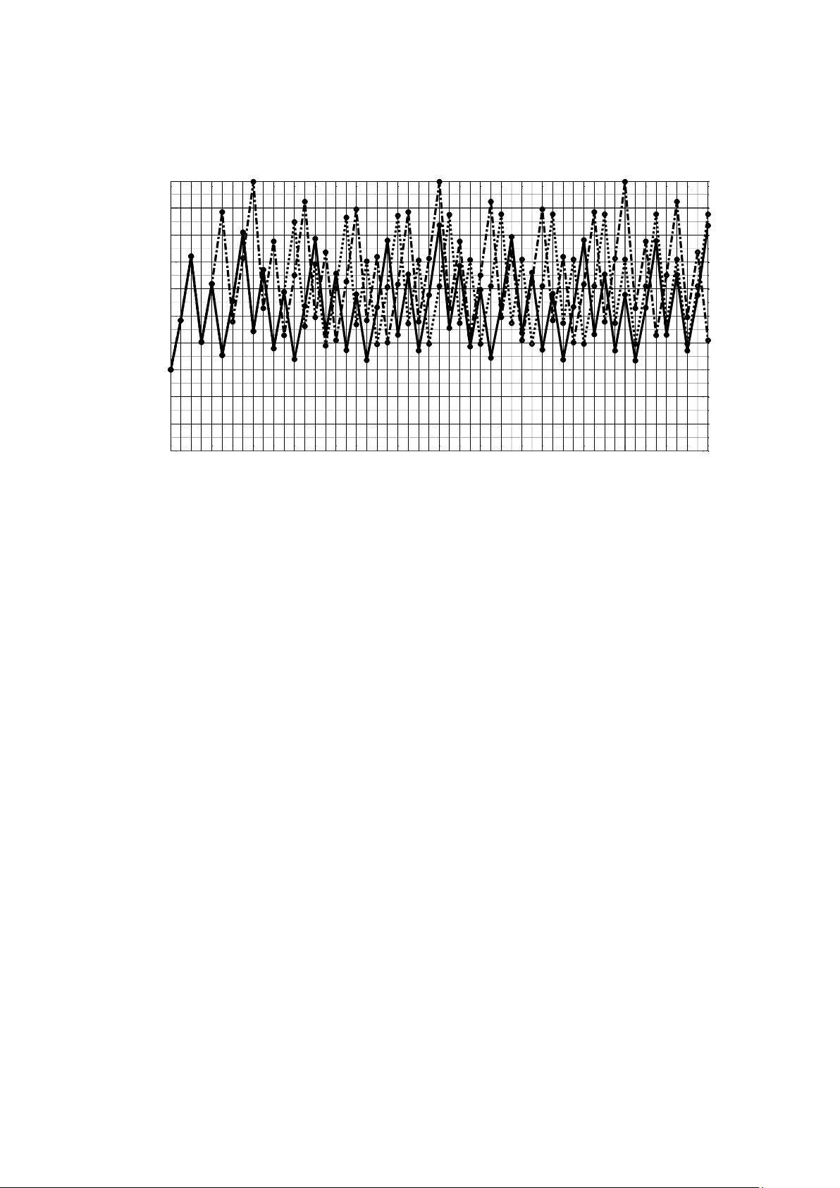
1 Efficient modeling of chemotherapy regi mens using mixed-integer linear progra mming Alain Billionnet Laboratoire CEDRIC, École N ationale Supérieure d’ Informatique pour l’Industrie et l’Entreprise, 1, square de la Résistance, 91025, Évry cedex, France email address : Alain.Billionnet@ensiie.fr Abstract In this article, we focus on determining a minimum -cost treatment program aimed at maintaining the size of a cancerous tumor at a level that allows the patient to live comfortably. At each predetermined point in a treatment horizon, the patient either receives drug treatment or does not. In the first case, the tum or shrinks and its size i s multiplied by a constant factor lower than 1; in the second, it grows following an exponential or Gompertz growth law. We first demonstrate that a simple heuristic solution provide s an optimal treatment program. We then show that th e Gompertz function can be de scribed, like the ex ponential function, b y a simple rec urrence relation that does not explicitly d epend on time. Thanks to the characteristics of the logarithmic function, this property allows us to formulate the problem as a mixed-integer linear progr am. This result makes it possible to solv e the problem ve ry efficiently using one of t he many solvers available to handle this t y pe of program, and above all to consider and solv e several ex tensions to the problem. In particular, we show how to determine which of the optimal e quivalent solutions to the initial problem a re the most relevant. We also show how to measure th e effect of a marginal increase in the treatment budget on patient qualit y of life. Numerous computational ex periments are presented to illustrate these issues. Keywords Treatment · Scheduling · Canc er · O ptimization · Tumor growth · Mixed-integer linear programming 1 Introduction The problem studied in this article is inspired by the reference (Bräutigam, 2024). In this article, the author is interested in determining a chemotherapy treatment program for cancer that achieves a g iven medical objective while being cost -effective. De termining a treatment schedule involves deciding when the treatment shoul d b e administered to the patient. It is assumed that we are dealing with a tum or which, without treatment, grows and, on the contrary, re gresses when t reatment is administ ered. Both tumor growth and tumor regression in response t o treatment are complex phenomena (Wodarz & Komarova, 2014). We assume that the models describing growth and regression are known deterministic models. This que stion of optimal tre atment planning is part of cancer res earch, a disease which, despite major advances, remains a serious affliction. R eaders can refer to (Bräutigam, 2024) 2 and the references therein for man y details and additions on the subject and also to (Shi et al., 2014), a comprehensive surve y o n optimization models conce rning ch emotherapy treatment planning in oncolog y. A s discussed in (Brautigäm, 2024), the search for a good treatment schedule can be carried out heuristically. The result is a solution that may be quite satisfactory, but it is not clear whether it differs significantl y from the optimal solution. In this article, we show th at, u nder certain conditions, a heuristic solut ion that comes naturally t o mind is optimal. An important issue in the search for appropriate solutions is that the problem under consideration generally admits several optimal solutions, i.e. of minimal cost, which are not at all equivalent from a medical point of view. We show in this article that the problem can be tackled quite effectively b y mathem atical programming, more specifically by mi xed- integer linear programming. This makes it possible, on the one hand, to determine which of the optimal solutions is the most interesting according to certain criteria and, on the othe r hand, to consider several relevant ex tensions of the initial problem. It is worth noting that numerous articles have b een published on how operations research can con tribute to the fight against cancer. These articles address issues relating to prevention, diagnosis, staging and treatment (Saville et al., 2018). 2 Presentation of the problem This work inspired b y the reference (Bräutigam, 2024) con cerns the scheduli ng of drug dose administration, over a certain tre atment h orizon, to cancer patients. This horizon is divided int o K periods of equal length (52 weeks, for example), at the start of which a drug dose ma y or ma y not be administered. It is assumed that we know how tumor size evolves over a p eriod: if no treatment is administ ered at t he start of the period, the size of the tumor increases over the period following a certain grow th function; if a treatment is administered at the start of the period, the size of the tumor decreases following a certain decay function . More precisely, i f we note k S the siz e of the tumor at th e beginning o f period k , we have 1 () kk S f S   if there is no treatment at the start of period k - 1 and 1 () kk S g S   if there is treatment. It is assumed that () f x x  and () g x x  for all x and that () fx and () gx are increasing functions. To simplify presentation, we make the assumption, as in (Bräutigam, 2024), that no treatment can be undertaken that would result in tumor siz e falling below a certain fixed threshold. W e will comment on this assumption at the end of Section 4. The problem is to determine the periods at the start of which a dose of d rug must be administered to maintain, over the entire horizon, the tumor siz e below a fix ed threshold and thus ensure a certain quality of li fe for the patient while minimizing the overall cost g enerated b y the 3 treatment over the horiz on considered. It is assumed here that the cost of one treatment is equal to p . 3 Under certain conditions, the heuristic solution is optim al A natural heuristic solution is to administer treatment at the start of period k if and onl y if, without treatment, the tumor size at the start o f period k +1 would ex ceed the tolerated size, S Tol . In other words, if S verifies () Tol f S S  , since the fun ction f is increasing, the h euristic solution is to administer treatment at the start of p eriod k if and onl y if k SS  . We'll show b y recurrence on k that if ( ( )) ( ( )) g f S f g S  then the heuristic solution is optim al. Let [] k CS be the minimum treatment c ost over periods k , k +1 ,..., K when the tumor size i s equal to S at the beginning of period k . According to Bellman's optimality principle (Bellman, 1953), 11 [ ] min{ [ ( )], [ ( )]} k k k C S C f S p C g S   (a) with constraints () Tol f S S  and min () g S S  . The function [] k CS is increasing Since f a nd g are incr easing functions, [] K CS is 0 if SS  and p if SS  . () K CS is therefore an increasing function of S . Assume that 1 [] k CS  is an increasing function and show that [] k CS is also increasing. According to (a), since f , g and 1 k C  are increasing functions of S , [] k CS , which is equal to the minimum of two increasing functions, is also an increasing function. Optimality of the heuristic solution Recurrence assumption: At the start of period k +1, the optimal decision is to apply the heuristic, i.e. if () Tol f S S  then 12 [ ) ] [ ( ] kk C C S f S   . We deduce 22 [ ( ] [ ( ] )) kk fp C g S C S   . This is obvious at the start of the last period. Let's show that, at the start of period k , the optimal decision is also to apply the heuristic, i.e. if () Tol f SS  then 1 [ ] [ ( )] kk CC f SS   . To do this, we have to show that if () Tol f SS  then 11 [ ( ] [ ( ] )) kk fp C g S C S   . Accordin g to the recurrence assumpti on, if ) ( () Tol f SS f  (which also implies ) ( () Tol f SS g  since f is increasing and ( ) ( ) g S f S  ) then 1 2 2 [ ] [ ( ] [ ) (] ( ) ( ) ( )) k k k C f S C f S C f p S fg       and 12 [ ] [ ( ] ( ) ( )) kk p C g S C pf gS     . The heu ristic solution is therefore optimal if ( ( )) ( ( )) g f S f g S  since we've shown that k C is increasing. This property can be interpreted as follows: let's consider a tumor of a certain 4 size at the start of p eriod k and assume that the following 2 strat egies are possible: 1) no treatment at the start of period k and tr eatment at the start of period k +1, 2) treatment at the start of p eriod k and no treatment at the start of period k +1. If ( ( )) ( ( )) g f S f g S  then the tumor siz e at the start of period k +2 will be smaller with strate gy 1 than with strateg y 2. W e'll see in Section 4 that this property is verified when the growth of the tumor size follows the exponential or Gompertz law, whereas its decrease consists in apply ing a multipl icative reduction factor. 4 General formulation of the problem by a mathematical program Although the heuristic solut ion is an optimal solution in the case where ( ( )) ( ( )) g f S f g S  , it is interesting to approach the problem by mathematical pro gramming. Indeed, as we shall see later, man y interesting extensions to the p roblem c annot be solved b y a heuristic method, but can be solved by mathematical progra mming. Bräutigam (2024) proposes several formulations of the problem in the form of a mathematical pro gram in the case where, on the one hand, tumor growth follows the exponential model (Collins, 1956 ) or the Gompertz model ( Laird, 1964 ; Gerlee, 2013; Benzekr y, 2014) and, on the other hand, the effect of treatment reduces tumor size by a constant factor. Bräutigam (2024) notes that solving these programs by the optimiz ation solver CP LEX ( IBM Inc, 2021) for the exponential model and b y BARON (Sahinidis, 1996) for the Gompertz model requires considerable computing time. The use of these programs is therefore limited and Bräutigam (2024) points out that this gives rise to the need for research to developing ways to improving computational performance . In this section, we begin b y expressing the tumor size at the start of period k as a general function of its size at the start of period k -1, based on the functions f and g from the previous section. This siz e at the s tart of period k naturall y depends on th e treatments administ ered at the sta rt of periods 1,2,..., k -1. Th en we will consider th e case where 11 ( ) ( ) kk f S S     and 11 ( ) ( 1 ) ( ) kk g S RF f S   where  and  are two positive coefficients and RF is the reduction factor associated with the treatment. As we will see in sections 6.1 and 6.2, the g rowth function f corresponds to the two case s considered by Bräutigam (2024): the exponential model when 1   and the Gompertz model when 01   . Thus, the evolution of tumor size between the beginning of period k -1 and the beginning of period k ob eys a multipli cative recurrence with a possible p ower. The fact that this recurrence does not explicitly depend on k for either tumor growth or tu mor decay will, as we shall see, make solving the pr oblem much easier. 5 Notation  Data { 1 , ..., } HK  : horizon considered composed of K periods of equal length (e.g. weeks); p : cost for a dose of treatment; S init : initial tumor size (at the beg inning of period 1); min S : minimum possible size of the tumor after trea tment; Tol S : maximum size of tumor tolerated; f : function describing tumor growth without treatment, 1 () kk S f S   ; g : function describing tumor decay with treatment, 1 () kk S g S   ; RF : tumor siz e reducti on coefficient after treatment , 1 ( 1 ) ( ) kk S RF f S   ; in this case ( ) ( 1 ) ( ) kk g S RF f S  .  Variables { 0 ,1 } ( ) k X k H  : B oolean variable that equals 1 if and only if a dose of treatment is administered at the beginning of period k ; m in , ( ) k k Tol S S S S k H      : variable representing tumor siz e at the beginning of period k , taking into account doses administ ered in previous periods; tumor size must always remain between two fixed extreme values, S min and S Tol . min , l o g ( ) log ( ) ( ) k k Tol LS S LS S k H      : logarithm of k S . According to the above and using Boolean v ariables X k which b y convention take the value 1 if and onl y if a t reatment is administered at the beginning of pe riod k , the tumor siz e at the start of period k , S k , is equal to 1 1 1 1 ( 1 ) ( ) [ ( )] k k k k X f S X g f S      . Indeed, th e tumor si ze at the start of period k is equal to 1 [ ( )] k g f S  if a dose of drug is administered at the start of period k -1, corresponding to 1 1 k X   , and to 1 () k fS  otherwise, corresponding to 1 0 k X   . Now consider the case where () f x x    and ( ) ( 1 ) g x RF x  . In this case, the previous ex pression for tumor size becomes 11 ( 1 ) ( ) k k k S RFX S     . Indeed, the tumor si ze at the start of period k is equal to 1 ( 1 ) ( ) k RF S     if a dose of dru g is administ ered at the start of period k -1, corresponding to 1 1 k X   , and to 1 () k S    otherwise, corresponding 6 to 1 0 k X   . Using the logarithmic function, we obtain the following equality: 11 log( ) log( 1 ) log( ) l og( ) k k k S RFX S       . Examining the two po ssible values of the variable 1 k X  , we s ee that 1 log ( 1 ) k RFX   is equal to log( 1 ) RF  if 1 1 k X   and 0 otherwise. We therefore have 11 log( 1 ) log( 1 ) kk RFX X RF     and the p revious equality is equivalent to the following equalit y 11 log( ) log( 1 ) l og( ) l og( ) k k k S X RF S       or, b y setting log( ) kk LS S  , to 11 log( 1 ) l og( ) k k k LS X RF LS       . The adva ntage of this last expression is it s lin ear natu re (as a function of the varia bles k LS ). The problem under consideration can therefore be formulated by the mixed-integer linear program P 1 . P 1 : 1 1 11 min min ( ) log( ) ( 1.1 ) log( 1 ) log( ) , 2 ( 1.2) s.t. , l og ( ) log( ) ( 1.3) { 0 ,1 } ( 1.4) K k k init k k k k k Tol k C X p X LS S LS X RF LS k H k LS S LS S k H X k H                            The economic function, () CX , expresses the cost of treatment since, b y convention, a dose of drug is administ ered at the start of period k if and onl y if 1 k X  . Constraint 1.1 states that the logarithm of the tum or size at the start of p eriod 1 is equal to log( ) init S . Linear cons traint 1.2 expresses the logarithm of the tumor siz e at the start of period k as a function of the logarithm of its size at period k -1, t he variable 1 k X  and the coefficients RF ,  and  . Constraints 1.3 and 1.4 specify the dom ain of variables k LS and k X . In conclusion, the probl em can be formulated b y a linear mathematical program wit h real variables and Bool ean variables in the case where 1) Tumor growth obeys the function () f x x    which is the case for the exponential or Gompe rtz model, 2) Tumor d ecay obeys the function ( ) ( 1 ) g x RF x  . This linear formulation will enable the problem to b e solved efficiently using one of the many mixed-integer linear programming solvers available. Remark To sim plify presentation , we h ave mad e the assumption, as in (Bräuti gam, 2024), that no treatment can be un dertaken that would reduce tumor size below a certain value. The following slightl y different constraint could easily be taken into account: a treatment can always be undertaken at the beginning of each period, but the size reached by the tum or as a result of this treatment ca nnot f all below a certain value. To take account of this slight 7 modification to the problem, it would suffice to replace the equality constrain t (1.2) by the inequality constraint 1 1 min ma x{ log( 1 ) l og( ) , log( )} k k k LS X RF LS S       . Some solvers, such as Gurobi (Gurobi Optimiz ation, 2023), handle this type of constraint directly. If using a solver that doesn't, thi s constraint can be linearized be forehand in a classic wa y, using new Boolean variables. 5 Model strengthening The f act that we can formulate the p roblem with mixed-integer linear programming in the case of the exponential model and the Gompertz model opens up the possibil ity of solvin g interesting extensions of the problem in these cases. We present several of these extensions below by wa y of example. We shall se e that they are easy to for malize from the basic program P 1 . 5.1 Combination therapy Combination therapy, a treatment modality that combines two or mo re therapeutic agents, is a particularly interesting approach to ca ncer therapy. Indeed, this approach c an have better ef ficacy than the mono-therapeutic approach due to s ynergistic or/and additive properties on the one h and, and reduce dru g resistance on the other h and (Mokhtari et al., 2017). W e will consider here the case where n t ypes of tumor tre atment a re av ailable and that one and onl y one of these treatments can potentially be administered at the start of each period. Let's assum e that type i treatment ( i =1,2,…, n ) costs p i and corresponds to a reduction factor i RF . Using the Boolean variable ( 1 , ..., ; 1 , ..., ) i k X k K i n  which, b y convention, is equal to 1 if and onl y if a treatment o f type i is admi nistered at the be ginning of period k , we can ex press k S as a function of 1 k S  as 11 1 ( 1 ) ( ) n ii k k k i S RF X S       as long as we impose the constraint 1 1 1 n i k i X     . Using the logarithmic function and noting the logarithm of k S by k LS as before, we obtain the following equality: 11 1 lo g( 1 ) log( ) n ii k k k i LS RF X LS         . Since 1 1 1 n i k i X     , 1 1 lo g( 1 ) n ii k i RF X     = 1 1 log( 1 ) n ii k i RF X     . Finally, the problem can be formulated by the program P 2 . 8 P 2 : 11 1 11 1 1 1 min min ' ( ) log( ) ( 2.1 ) log( 1 ) log( ) , 2 ( 2.2) s.t. 1 ( 2.3 ) , l og( ) log( ) ( 2.4) { 0 ,1 } , 1 , ..., ( 2.5) Kn i ik ki init n ii k k k i n i k i k k Tol i k C X p X LS S LS RF X LS k H k X k H LS S LS S k H X k H i n                                        5.2 Spacing between treatments Time int erval to treatment is an im portant qu estion (Yoo et al., 201 7). It can be interesting, say, to have s olutions that ensure a minim um spacing between two treatments. For example,  treatment-free periods can be imposed between two tre atment p eriods. Thus, if a treatment takes pla ce at the start of period k , there can be no tr eatment at the start of periods k +1, k +2, k +  . Of course, respecting these treatment intervals can increase the ov erall cost o f treatment. Under this constraint, the problem can be for mulated as program P 3 . P 3 : 1 11 12 min min ( ) log( ) (3.1 ) log( 1 ) log( ) , 2 (3.2) ... ( 1 ) 1 , ..., (3.3 ) s.t. , l og( ) log( ) (3.4) { 0 ,1 } (3.5 ) init k k k k k k k k k Tol k CX LS S LS X RF LS k H k X X X X k K LS S LS S k H X k H                                       Let's look at constraint (3.3 ). If a treatment is administered at the be ginning of period k , then 1 k X  and the second member of the constraint equals 0. This implies 12 ... 0 k k k X X X         . Otherwise, the second member of the constraint equa ls  and the constraint becomes inactive. Note that the formulation of the problem by the mathematica l program P 1 also makes it easy to take into account the fact that certain trea tment dates may b e imposed a priori, for example at the beginning of the 10th week and at t he beginning of the 20th. To do this, simply add the constraints 1 k X  to the progra m for the relevant values of k . 5.3 Minimizing maximum tumor size It may be of interest to determine a treatment schedule that minimizes the maximum tumor size over the time horizon under consideration, while remaining below a certain cost. 9 This question can be associated with each of the 3 precedin g probl ems, formulated as P 1 , P 2 and P 3 , which themselves aim to minimiz e cost while ensuring that the tumor does n ot grow beyond a certain size. For P 1 , P 2 and P 3 this problem can be formulated by replacing in thes e programs the economic function to be minimized by the non-n egative real variable LS and adding the constraint () k LS LS k H  . For P 1 and P 3 , the constraint k kH pX C    must also be added, and fo r P 2 the constraint 11 Kn i ik ki p X C    where C denotes the cost not to be exceeded. 1 () C  , 2 () C  and 3 () C  are the programs obtained. 1 1 min (1.1) (1.2) (1.3) (1.4) ( ) : s.t. () K k k k LS C pX C LS LS k H LS                     2 11 min (2.1) (2.2) (2.3) (2.4) (2.5) ( ) : s.t. () Kn i ik ki k LS C p X C LS L S k H LS                     3 1 min (3.1) (3.2) (3.3) (3.4) (3.5) ( ) : s.t. () K k k k LS C pX C LS L S k H LS                     In an optimal solution of () i C  , i =1,2,3, the maximum size reached b y the tumor during horizon H is equal to * LS e whe re L S * de signates the optimum value of () i C  , i.e. the optimum value of variable LS . In addition, since the program P 1 (resp. P 2 , P 3 ) generally has several optimal solutions, it may be of particular int erest to d etermine from among these optimal solutions, the one that minimizes the maximum siz e taken by the tumor over the horizon under consideration. The program 1 () C  (resp. 2 () C  , 3 () C  ) can b e u sed to determine this p articular opti mal solut ion. To do this, simpl y solve 1 () C  (resp. 2 () C  , 3 () C  ), giving C the optimal value of P 1 (resp. P 2 , P 3 ). 6 Experiments In this section, we present experiments to solve the program s P i and () i C  , i =1,2,3. Section 6.1 deals with the exponential tum or growth model and section 6.2 with the Gompertz model. In these two sections, the effect of treatment is to reduce tumor size by a factor of RF . All the experiments presented in this article were carried out usin g the mathematical programming lan guage AMPL (Fourer and Gay, 1993), version 2022 - 10 -13, to model the different pro grams and Gurobi (Gurobi Optimization, 2023), version 10.0.1, a commercially 10 available mathematical program solver based on the most efficient al gorithms available today, to solve them. Gurobi can solve line ar and non -linear pro grams invol ving both re al and integer variables . The experiments have be en per formed on a PC with an Intel Core i7 1.90 GHz processor with 16 Go RAM. 6.1 Exponential model In this section, we consider the case where tumor growth follows the exponential distribution given b y : 0 () bt te   , where () t  is the value of the function  at time t , 0  is its value at time t =0 , b is a positive coefficient expressing the growth rate and e is the base of the natural logarithm. I t is generall y a ccepted that in the earl y stages, tumor growth can be approximated by an exponential function (Retsky et al. 1990). It is assumed here and in all that follows that the unit of time is the period. It is known (and easy to demonstrate) that, in the exponential case, if the size of the tumor at the start of period k is equal to k S then, without treatment, its size will be equal to k S  at the start of p eriod k +1 with log( ) b   . W e are clearl y within the framework considered, 1 () kk SS     , b y posing log( ) b   and 1   . It's eas y to check that i n this case, b ased on the results of Section 3, the heuristic solution is optimal. This is because 2 ( ( )) ( ( )) ( 1 ) k k k g f S f g S RF S     . Table 2 presents numeri cal experiments on solvi ng P 1 (resp. P 2 , P 3 ) and 1 () C  (resp. 2 () C  , 3 () C  ), giving C the optimal value of P 1 (resp. P 2 , P 3 ) for the latter three pro grams. The values of the various parameters used in the formulation of these programs, taken from (Bräutigam, 2024) with the exception of RF 1 , RF 2 , p 1 and p 2 , are presented in Table 1. The horizon considered is composed of 52 periods. Table 1 Parameter values for the treatment planning problem in the case of ex ponential tumor growth (Bräutigam, 2024) Tumor growth function parameters S init S Tol S min RF RF 1 RF 2 p p 1 p 2  0 50   , 1.5 be   log( ) 1.5 b   50 500 10 0.6 0.6 0.7 10 10 13 1 Comments on Table 2 First column : S olving each of the 3 programs is instantaneous. It required less than one second of computation. The resolution of P 1 provides a treatment schedule with a cost of 210. With this schedule, the maxim um size reached by the tumor durin g the horiz on considered is 11 equal to 496.46 and is therefore ver y close to the tolerated siz e ( S Tol =500). We may ask whether P 1 admits other optimal solutions and in particular solutions for which the maximum size reached by the tumor is smaller. Solving 1 () C  with C =210 answers this question b y providing a treatment schedule, still costing 210, but with a maxim um tumor size equal to 315.48. This solution seems much more interesting than the first (at equal cost) in terms of the patient's qualit y of life, since it enables tum or size to be maintained at a much lower value. There is also the qu estion of whether an additional treatment dose si gnifican tly influences the maximum tumor siz e reached. The resolution of 1 () C  with C =220 answers this question b y providing a treatment schedule that k eeps the tumor size below a much smaller value (126.19). An additional dose of treatment is therefore ver y effective in thi s case, if the aim is to keep the tumor siz e as small as possible. These 3 solut ions are shown in Figure 1. W e can also see that solving P 1 provides fa irly re gular treatment frequencies, since between two treatment periods there i s always at least one without treatment and at most two. This is not the case for the optimal solut ion of 1 () C  with C =210 and also with C =220. In both cases, there are at least two consecutive periods with treatment and 4 or 6 consecutive periods without treatment betwe en two treatment periods. Treatment schedulin g is therefore much more irregular. Programs P 3 and 3 () C  take this aspect of the problem into account. Second column : The resolution of P 2 and 2 () C  - with 2 possible types of treatment - is instantaneous. Wit h the values chosen for the cost of treatments, the optimal treatment schedule includes, in the 3 cases examined (P 2 , 2 ( 204 )  , and 2 ( 217 )  ), a comparable number of t ype 1 and type 2 treatments. On the other hand, treatments are not administered on a regular basis. In all 3 cases, there a re at least tw o consecutive periods with treatment and 4 or 6 consecutive periods without treatment betwe en two treatment periods. The resolution of P 2 provides a solution of cost 204 with a maximum tumor size equal t o 493.50. Resolving 2 ( 204 )  does not reduc e this size. On the other hand, if we accept an additional trea tment, either type 1 or type 2, the maximum tumor siz e over the tr eatment horizon decrease s considerably, from 493.50 to 148.05. Third column : Resolution of P 3 and 3 () C  is instantaneous. The cost of the optimal solution of P 3 and the max imum tumor size reached in this solution are identical to thos e of the solution of P 1 . And so, as expected, imposing the additional constraint (compared with P 1 ) of having a treatment-free period between two tre atment periods does not increase the value of 12 the optimal solution or the maximum value of the tumor size. On the other hand, the addition of thi s constraint leads to a different solution to that obtained with P 1 , insofar as the re is greater irregularity in the administration of treatments (8 periods withou t treatment between two treatments). The solut ions of 3 ( 210 )  and 3 ( 220 )  are identi cal to those of 1 ( 21 0)  and 1 ( 22 0)  in terms of maximum tum or size. On the other hand, it provides much greater regularity in treatment administration. Table 2 Experimental results for solving the programs P 1 , P 2 , P 3 , 1 () C  , 2 () C  and 3 () C  in the case of exponential tumor growth P 1 P 2 P 3 Minimum cost: 210 Maximum tumor size: 496.46 Min. spacing between 2 treatments: 1 Max. spacing between 2 treatments: 2 Computation time: <1s. Figure: 1 Minimum cost: 204 Number of type 1 treatments: 10 Number of type 2 treatments: 8 Maximum tumor size: 493. 50 Min. spacing between 2 treatme nts: 0 Max . spacing between 2 treatments: 5 Computation time: <1s. Minimum cost: 210 Maximum tumor size: 496.46 Min. spacing between 2 treatme nts: 1 Max. spacing between 2 treatments: 8 Computation time: <1s. 1 ( 21 0)  2 ( 204 )  3 ( 210 )  Maximum tumor size: 315.48 Min. spacing between 2 treatme nts: 0 Max. spacing between 2 treatments: 6 Computation time: <1s. Figure: 1 Number of type 1 treatments: 10 Number of type 2 treatments: 8 Maximum tumor size: 493.50 Min. spacing between 2 treatments: 0 Max. spacing between 2 treatments: 5 Computation time: <1s. Maximum tumor size: 315.48 Min. spacing between 2 treatme nts: 1 Max. spacing between 2 treatments: 3 Computation time: <1s. 1 ( 22 0)  2 ( 217 )  3 ( 220 )  Maximum tumor size: 126.19 Min. spacing between 2 treatme nts: 0 Max. spacing between 2 treatments: 4 Computation time: <1s. Figure: 1 Number of type 1 treatments: 10 Number of type 2 treatments: 9 Maximum tumor size: 148.05 Min. spacing between 2 treatme nts: 0 Max. spacing between 2 treatments: 6 Computation time: <1s. Maximum tumor size: 126.19 Min. spacing between 2 treatme nts: 1 Max. spacing between 2 treatments: 2 Computation time: <1s. 13 Fig. 1 Tumor size at th e beginning o f ea ch period for the optimal solution of P 1 (cost 210, dash-dotted line), for th e optimal solution of 1 ( 21 0)  (dotted line) and for the optimal solution of 1 ( 22 0)  (solid line). I n the solution of P 1 , the maximum tumor size is equal to S 27 =496.46, in the solution of 1 ( 21 0)  it is equal to S 53 =315.48 and in the solution of 1 ( 22 0)  it is equal to S 53 =126.19. 6.2 Gompertz model In this section, we consider the case where tumor growth follows the Gompertz function. This model is frequently used to model tumor growth in biolog y and medicine as a function of time (Benzek ry, 2014 ; Pitchaimani, 2014). It d escribes rapid ini tial tumor growth, which gradually slows as it approa ches an asymptotic si ze. There are se veral equivalent expressions. W e have adopted the one used b y Bräutigam (2024): ( 1 ) 0 () bt a e b te     where () t  represents the value of the function at time t , 0  its value at t =0 and a and b are two positive constants that control the growth rate and the shape of the associated curve. Let us express k S as a function of 1 k S  : ) ( 1) ( 1 ) ( 1 ) 1 0 0 // bk b k aa ee bb kk S S e e        ( 1) ( )( 1 ) b k b a ee b e      . S ince ( 1) 10 / bk aa e bb k S e e     , we get ( 1 ) 1 0 1 ( / ) b a e b k k k S S e S      = ( 1 ) 10 ( ) ( ) bb a ee b k Se     . We are therefore in the case wh ere 11 ( )= ( ) kk f S S    by posing ( 1 ) 0 () b a e b e     and b e    . Let's ch eck that in this case the h euristic solution is opti mal. 1 3 5 7 9 11 13 15 17 19 21 23 25 27 29 31 33 35 37 39 41 43 45 47 49 51 53 0 50 100 150 200 250 300 350 400 450 500 k S k cos t= 210 cos t= 210 cos t= 220 14 2 1 ( ( )) ( 1 ) [ ( ) ] ( 1 ) ( ) k k k g f S RF S R F S             , ( ( )) [( 1 ) ( ) ] kk f g S RF S    2 1 ( 1 ) ( ) RF Sk       . We therefore have ( ( )) ( ( )) kk g f S f g S  if 1 ( 1 ) RF RF     , i.e. if log( 1 ) log( 1 ) RF RF     . This last inequality is verified if 1   , which is indeed the case since b e    . Table 4 presents numeri cal experiments on solving P 1 (resp. P 2 , P 3 ) and 1 () C  (resp. 2 () C  , 3 () C  ) giving C th e optimal value of P 1 (resp. P 2 , P 3 ) for the l atter three pro grams. The values of the various parameters used in the formulation of these programs, taken from (Bräutigam, 2024) with the exception of RF 1 , RF 2 , p 1 and p 2 , are presented in Table 3. The horizon considered is composed of 52 periods. Table 3 Parameter values for Gompertz tumor growth experiments (Bräutigam, 2024) Tumor growth function parameters S init S Tol S min RF RF 1 RF 2 p p 1 p 2 0 50   a= 0.72 b =0.18 ( 1 ) 0 ( ) 3.68 b a e b ge       , 0.84 b e    150 500 60 0.6 0.6 0.7 10 10 13 Table 4 Experimental results for solving the programs P 1 , P 2 , P 3 , 1 () C  , 2 () C  and 3 () C  in the case of tumor growth following Gompertz's law P 1 P 2 P 3 Minimum cost: 200 Maximum tumor size: 499.09 Min. spacing between 2 treatme nts: 1 Max. spacing between 2 treatments: 2 Computation time: <1s. Figure: 2 Minimum cost: 191 Number of type 1 treatments: 10 Number of type 2 treatments: 7 Maximum tumor size: 499.09 Min. spacing between 2 treatme nts: 1 Max. spacing between 2 treatments: 3 Computation time: 29s. Minimum cost: 200 Maximum tumor size: 498.87 Min. spacing between 2 treatme nts: 1 Max. spacing between 2 treatments: 3 Computation time: <1s. 1 ( 20 0)  2 ( 19 1 )  3 ( 200 )  Maximum tumor size: 438.42 Min. spacing between 2 treatme nts: 1 Max. spacing between 2 treatments: 2 Computation time: <1s. Figure: 2 Number of type 1 treatments: 10 Number of type 2 treatments: 7 Maximum tumor size: 493.41 Min. spacing between 2 treatme nts: 1 Max. spacing between 2 treatments: 2 Computation time: 36s. Maximum tumor size: 438.42 Min. spacing between 2 treatme nts: 1 Max. spacing between 2 treatments: 2 Computation time: <1s. 1 ( 21 0)  2 ( 204 )  3 ( 210 )  Maximum tumor size: 418.02 Min. spacing between 2 treatme nts: 1 Max. spacing between 2 treatments: 2 Computation time: 3.2s. Figure: 2 Number of type 1 treatments: 19 Number of type 2 treatments: 1 Maximum tumor size: 435.78 Min. spacing between 2 treatme nts: 1 Max. spacing between 2 treatments: 2 Computation time: 70s. Maximum tumor size: 418.02 Min. spacing between 2 treatme nts: 1 Max. spacing between 2 treatments: 2 Computation time: <1s. 15 Comments on Table 4 First column : All 3 programs were solved very f ast. Solving P 1 and 1 () C  with C =200 took less than a second, while solving 1 () C  with C =210 took 3.2 seconds. The resolution of P 1 provides a tr eatment s chedule with a cost of 2 00. With this schedule, the maxim um size reached b y the tumor during the horizon considered is e qual to 499.0 9 and is therefore roughly equal to the tolerated size ( S Tol =500). We ma y ask whether P 1 admits other optimal solutions and in particular solutions for which the maximum size reached by the tumor is smaller. Solving 1 () C  with C =200 answers this question b y providing a trea tment schedule, still costing 20 0, but with a maximum tumor size equal to 438.42. This solution is slightly more attractive than the first (at equal cost) in terms of patient quality o f l ife, since it enables tumor siz e to be maintained at a sli ghtl y lower va lue. There is also the questi on of whether an additional treatment dose significantly influences the ma ximum tumor size reac hed. The resolution of 1 () C  with C=210 answers this question by providing a treatment regimen that keeps tumor size below a slightly smaller value (418.02). The value of an a dditional treat ment dose is therefore limited in this case, if th e aim is to keep tumor size as small as possible. These 3 solutions are s hown in Figure 2. We can also s ee that solving P 1 , 1 ( 20 0)  and 1 ( 21 0)  provides fai rly regular treatment f requencies, since betw een two treatment periods there is always at least one without treatment and at most two. Second column : Resolution of each of th e 3 p rograms - with 2 possible t ypes of t reatment - is no longer instantaneous, but is still very fast. Wit h the values chosen for treatment costs, the optimal tre atment plan includes, in the 2 c ases P 2 a nd 2 ( 19 1 )  , a relatively comparable number of type 1 and t ype 2 treatments. However, th is is not the case for 2 ( 204 )  , since of the 20 treatments admi nistered, onl y one is type 2. On the other h and, treatments are administered on a regular basis since between two treatment periods ther e is alwa ys at least one without treatment a nd at most two or three . The resolution of P 2 provides a solution of cost 191 with a maximum tumor size equal to 499.09. The resolution of 2 ( 19 1 )  barely reduces this siz e. On the other hand, if we accept an additional treatment, either t ype 1 or type 2, the max imum tumor size over the treatment horizon decreases slightly, from 493.41 to 435.78. Third column : Resolution of each of the 3 progr ams is inst antaneous. W e obtain ex actl y the same results as in column 1, which is not surprising sinc e the 3 solut ions in column 1 alread y 16 respect the spa cing constraint between two treatments imposed in programs P 3 , 3 ( 200 )  and 3 ( 210 )  . Fig. 2 Tumor size at th e beginning o f ea ch period for the optimal solution of P 1 (cost 200, dash-dotted line), for th e optimal solution of 1 ( 20 0)  (dotted line) and for the optimal solution of 1 ( 21 0)  (solid line). I n the solution of P 1 , the maximum tumor size is equal to S 9 =499.09, in the solution of 1 ( 20 0)  it is equal to S 53 =438.42 and in the solution of 1 ( 21 0)  it is equal to S 27 =418.02. 7 Discussion and perspective In this article, we look at the plannin g of a cancer treatment ov er a given t ime horizon. The treatment consists of administering a dose of medication to the patient at certain points on the horiz on. I t is assumed that, in the absence of treatment, the tum or increases in size over time according to a c ertain growth law and, conversely, that treatment leads to a ra pid reduction in tumor size according to a certain decay law without getting below a certain value. The problem considered b y Bräutigam (2024) and studied in this article is to determine when treatment shoul d be administered in order to ke ep tumor siz e below a certain threshold while minimizing the total cost of treatment. Following Bräutigam, w e approached the problem using mathematical programming, a branch of mathematics c oncerned with modeling and solvi ng optimization problems. W e have shown that if tumor growth follows an ex ponential or Gompertz law and decay consists of applying a constant r eduction factor, the problem can be formulated b y a mix ed-integer linear program, or more precisel y, by a line ar program with non -negative real variables and Boolean variables. Note that this is a “direct” linear f ormulation obtained using the lo garith mic 1 3 5 7 9 11 13 15 17 19 21 23 25 27 29 31 33 35 37 39 41 43 45 47 49 51 53 0 50 100 150 200 250 300 350 400 450 500 k S k  cos t= 200  cos t =200  cos t= 210 17 function and not a linearization of a nonlinear problem obtained by known linearization methods, which generally increase the numb er of variables and/or constraints. This result enabled us to solve the problem very efficientl y, using one of the many so lvers available for mixed-integer linear programs. Indeed, current solvers can solve large instances of this ty pe of program without difficulty. The fact that we were able to efficientl y solve the problem under con sideration has enabled us to consider and successfull y solve several interesting extensions. The first is to determine, from amon g all the tre atment schedules that allow tumor siz e to be kept below a certain threshold at the lowest cost, the one that minimizes the size reached b y the tumor ove r the horizon considere d. Experiments showed that this constraint made it possible in certain cases to d etermine a particularly interestin g schedule insofar as it enabled tum or size to be maintained at a much lower value than with the schedule determined wit hout this constraint. This extension also makes it possible to measure precisely th e marginal effect of increased treatment costs. In some cases an additional treatment dose considerably reduces the maximum tumor siz e over the ho rizon considered. Another ex tension of the initial problem is to consider the possi bility of havin g several possible types of treatment. These extensions are easy to formulate f rom the initial problem formulation. This is one of the well -known advantages of mathematical programming: it is p articularly e asy to appro ach vari ants of an initial problem b y adding/removing variables and/or constraints, which is not the case when the problem is approached by a specific algorithm. It should be noted, however, that “modeling” a problem using mathematical programming is not synonymous with “solving” it . Indeed, computation times can b e prohibitive. T he efficient resolution of the problem also means that it can be sol ved with a much larger number of periods. Generally speaking, the fact that we can solve the considered problem very efficientl y gives us hope that we'll be able to solve problems of the same type, but which are more complicated because the y are closer to real-life situations. Being able to express the siz e of the tum or at the start of period k , S k , as a f unction of it s size at the start of period k -1, S k -1 , by the recurrence relations 1 () kk SS     if there is no treatment at the start of period k -1 and 1 [ ( ) ] kk SS     otherwis e is the key point enabling the problem to be formulated b y a linear program and therefore the key point for it s efficient solution. As we have see n, the growth and deca y functions considered in this article – and in (Bräutigam, 2024) – allow these expressions. 18 Other growth and de c ay functions may also need to be taken int o account in a real-life context. Indeed, the effe ct of tr eatment on tumor size may be more complex than what we have considered. For example, the tumor dec ay caused b y treatment may follow the inv erse Gompertz function, which takes into ac count a slowdown in decay over time. Thus tum or decay would verify the equality 1 [ ( )] kk S f S     instead of 1 ( 1 )[ ( )] kk S RF f S   where  and  are constants. It can be shown that in this case - tumor growth always following an exponential or Gompertz law - the determination of an optimal treatment schedule can be formulated b y a quadratic mathematical program. To solve it, the program must either be linearized, or one of the many ef ficient commercial solvers that can handle mixed -integer quadratic programs directly must be used. Note also that in the case where we are interested in growth functions that ca nnot be ex pressed exactly b y the equa lity 1 () kk SS     - as is the case, for example, with the Be rtallanfy model (Bertallanfy, 1957) - it is possible to approach the problem by approximating these growth functions by such an expression. Declarations The author has no relevant financial or non-financial interests to disclose. No funding was received to assist with the preparation of this manuscript. References Bellman, R.E. (1953). An introduction to the theory of dyna mic pro gramming.The Rand Corporation, Santa Monica, CA, Document Number R-245. Benzekry, S., Lamont, C., Beheshti, A., Tracz, A., Ebos, J .M.L., Hlatk y, L., & H ahnfeldt, P. (2014). Classical mathematical models for description and prediction of experimental tumor growth (2014). PLOS Computational Biology,10 (8), e1003800. https://doi.org/10.1371/journal.pcbi.1003800 Bertalanffy, L.v. (1957). Quantitative laws in metabolism and growth. The Quarterly Review of Biology, 32 (3), 217 – 231. https://www.journals.uchicago.edu/doi/pdf/10.1086/401873 Bräutigam, K. (2024). Optim ization of chemotherapy regimens using mathematical programming. Computers & Industrial Engineering,191,110078 . https://doi.org/10.1016/j.cie.2024.110078 Collins, V.P. et al. (1956). Observations on growth rates of human tumors. Am. J. Roentgenol. Radium Ther. Nucl. Med. 76 , 988 – 1000 Fourer, R., Ga y, D. M., & Ke rnighan, B. W . (1993). AMP L, a modeling lan guage for mathematical programming. Boyd & Fraser Publishing Company. 19 Gerlee, P. (2013). The model muddle: in search of tum or growth laws. Cancer Res. 73 (8), 2407-2411. https://doi.org/10.1158/0008-5472.CAN-12-4355 . Gurobi Optimization, LLC. (20 23). Gurobi optimi zer reference manual. Version 9.0. Gurobi Optimization, LLC. https://www.gurobi.com Laird, A.K. (1964). Dynamics of tumor growth. Br. J. Cancer, 13 (3), 490-502. https://doi.org/10.1038/bjc.1964.55 Mokhtari, R. B., Homa youni, T. S., Baluch, N., Morgatskaya, E., Kumar, S., Das, B., & Yeger, H. (2017). Combination therapy in combating cancer. Oncotarget, 8 , 38022-38043. https://www.oncotarget.com/article/16723/text/ Pitchaimani, M., & Ori, G.S. (2014). Stabilit y anal ysis of Gompertz tumour growth model parameters. (2014). Journal of advances in mathematics, 7(3), 1293-1304. https://doi.org/10.24297/jam.v7i3.7253 Sahinidis, N.V. (1996). BARON: A general purpose global optimization software package. Journal of Global Optimization, 8 , 201-205. https://doi.org/10.1007/BF00138693 Saville, C. E., Smith, H. K., & Bijak, K. (2018). Operational research techniques applied throughout cancer care services: a review . Health Systems , 8 (1), 52 – 73. https://doi.org/10.1080/20476965.2017.1414741 Shi, J., Alagoz, O., Erenay, F.S. et al. (2014). A surve y of optimization models on cancer chemotherapy treatment planning. Annals of Operations Research, 221 , 331-356. https://doi.org/10.1007/s10479-011-0869-4 Yoo, T.K., Moon, H.G., Han, W., & Noh, D.Y. (2017). Time interval of neo adjuvant chemotherapy to surgery in breast ca ncer: how long is acceptable? Gland Surg, 6 (1), 1-3. https://doi.org/10.21037/gs.2016.08.06 Wodarz, D., & Komarova, N. L. (2014). D ynamics of cancer: mathemat ical found ations of oncology. World Scientific Publishing Co. Pte. Ltd.