Policy-Controlled Generalized Share: A General Framework with a Transformer Instantiation for Strictly Online Switching-Oracle Tracking

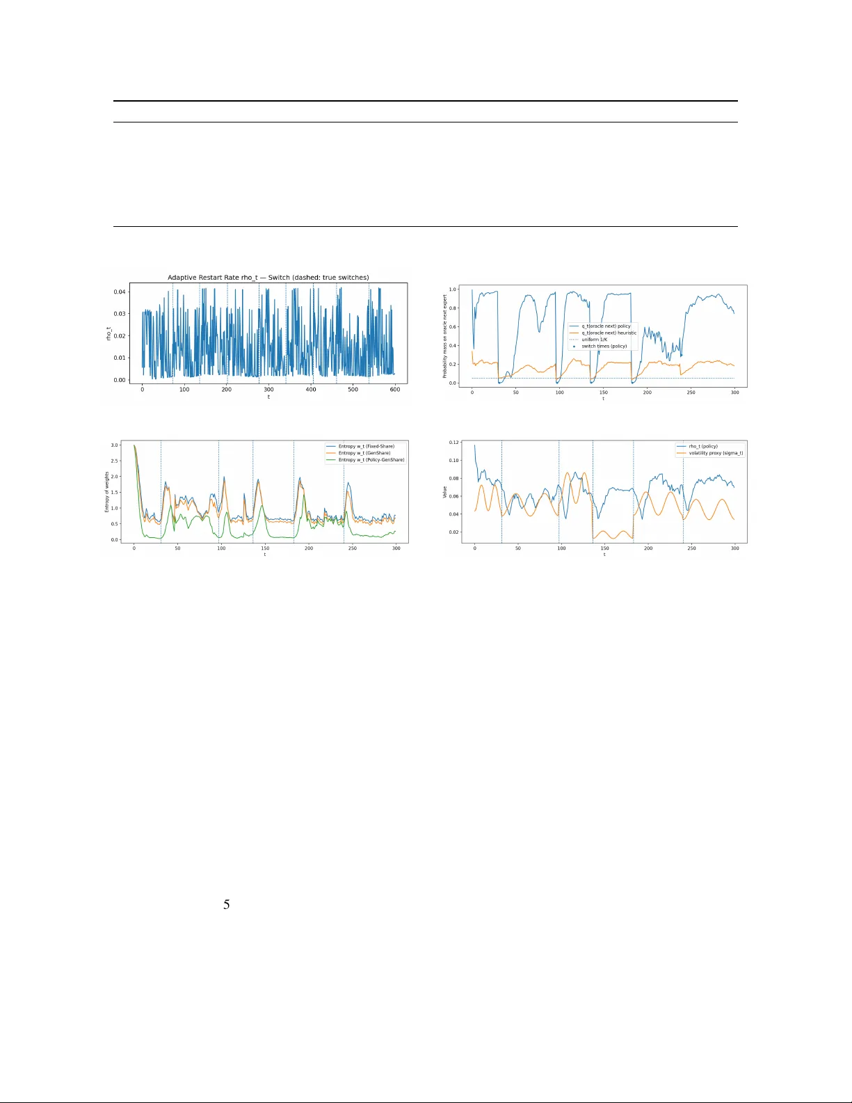
P O L I C Y - C O N T R O L L E D G E N E R A L I Z E D S H A R E : A G E N E R A L F R A M E W O R K W I T H A T R A N S F O R M E R I N S T A N T I A T I O N F O R S T R I C T L Y O N L I N E S W I T C H I N G - O R A C L E T R A C K I N G Hongkai Hu Antai College of Economics and Management Shanghai Jiao T ong Univ ersity if-only@sjtu.edu.cn A B S T R AC T Static regret to a single expert is often the wrong target for strictly online prediction under non- stationarity , where the best expert may switch repeatedly over time. W e study P olicy-Contr olled Generalized Shar e (PCGS), a general strictly online framew ork in which the generalized-share recur- sion is ﬁxed while the post-loss update controls are allo wed to vary adaptiv ely . PCGS separates the analysis of the share backbone from the design of the controller . Its principal instantiation in this pa- per is PCGS-TF , which uses a causal T ransformer as an update controller: after round t ﬁnishes and the loss vector is observed, the T ransformer outputs the controls that map w t to w t +1 without altering the already committed decision w t . Under admissible F t -measurable update controls, we obtain a pathwise weighted regret guarantee for general time-varying learning rates, and a standard dynamic- regret guarantee against any expert path with at most S switches under the constant-learning-rate specialization. In both cases, the switching term depends directly on  t : π t +1  = π t − log q t ( π t +1 ) , making restart allocation part of the certiﬁed difﬁculty of tracking a switching comparator . Empir- ically , all results labeled PCGS-TF correspond to this T ransformer-controlled instantiation. On a controlled synthetic suite with exact DP switching-oracle ev aluation, PCGS-TF attains the lo west mean dynamic regret in all sev en non-stationary families and its advantage increases with larger expert pools. On a reproduced household-electricity benchmark, PCGS-TF also attains the lo west normalized dynamic regret for S ∈ { 5 , 10 , 20 } . K eywords strictly online learning; non-stationary time series; prediction with expert advice; switching oracle; dynamic regret; Fixed Share; Generalized Share; strictly causal update control; restart distribution; causal T ransformer controller; in-context algorithm control; heavy tails and jumps; robust clipping; reproducibility 1 Introduction 1.1 Problem setting and metric W e study prediction with expert advice under a strictly online protocol. At each round t ∈ { 1 , . . . , T } , the learner must commit to a probability distribution w t ∈ ∆ K where ∆ K ≜  w ∈ R K + : K  k =1 w ( k ) = 1  , before observing the current loss vector ℓ t = ( ℓ t, 1 , . . . , ℓ t,K ) ∈ [0 , 1] K . The incurred loss is the mixed loss h w t , ℓ t i = K  k =1 w t ( k ) ℓ t,k , and the learner may update its internal state only after the round has been completed. This temporal ordering is essential: it rules out any use of ℓ t in the construction of w t and therefore enforces a genuine online, rather than one-step-delayed ofﬂine, ev aluation regime. The classical benchmark in expert advice is static regret with respect to the single best expert in hindsight. That metric is appropriate when the environment is effecti vely stationary , or when one is willing to compare against a ﬁxed action chosen after observing the entire sequence. In the present setting, howe ver , the identity of the best expert may ev olve over time: it may drift gradually , change abruptly at regime boundaries, or alternate repeatedly among different specialists. In such en vironments, comparison to a single static expert is often too coarse to capture the real difﬁculty of the task. A learner that tracks regime changes well may still exhibit large static regret simply because no single expert is uniformly best over the whole horizon. For this reason, the natural comparator class is not a ﬁxed expert but a switching path of experts. Let π 1: T ∈ [ K ] T denote a comparator path, where π t is the expert chosen at time t , and let #sw( π ) = T  t =2 1 { π t 6 = π t − 1 } be the number of switches in that path. For a switch budget S ∈ { 0 , . . . , T − 1 } , one considers the oracle value L sw T ( S ) ≜ min π : #sw ( π ) ≤ S T  t =1 ℓ t,π t , and ev aluates the learner through the corresponding dynamic regret DynRegret S ≜ T  t =1 h w t , ℓ t i − L sw T ( S ) . This metric explicitly quantiﬁes the price of adaptation relativ e to a comparator that is allowed a controlled amount of non-stationarity . It is therefore the right target when the main challenge is not prediction against a ﬁxed latent regime, but rapid tracking of a sequence of changing best experts. 1.2 Limits of ﬁxed restart schemes A canonical baseline for online expert aggregation is Hedge, or exponential weights, which is well known to enjoy optimal worst-case guarantees for static regret. Its appeal is undeniable: the update is simple, computationally efﬁcient, and supported by a clean minimax theory . Howe ver , the geometry of multiplicative updates also induces a structural limitation in non-stationary en vironments. Once the weight assigned to an expert becomes very small, that expert can recov er only gradually under subsequent multiplicativ e reweighting, even if it later becomes optimal. In other words, the posterior may become excessi vely committed to a regime that has already ended. Share-type algorithms were introduced precisely to address this recov erability problem. Rather than relying solely on multiplicativ e reweighting, they inject a portion of probability mass back into the expert pool after each round. In Fixed Share, the amount of restarted mass is constant and the restart distribution is typically uniform. Generalized Share extends this basic mechanism by allowing greater ﬂexibility in how restart mass is redistributed. The conceptual lesson is that, in changing environments, good performance depends not only on identifying which experts performed well on the current round, but also on maintaining the capacity to reallocate mass efﬁciently when the underlying regime changes. This perspectiv e immediately suggests that a ﬁxed restart rule is unlikely to be uniformly adequate across hetero- geneous non-stationary regimes. If the environment is locally stable, aggressive restart may introduce unnecessary diffusion and slow concentration. If the en vironment undergoes abrupt changes, insufﬁcient restart can leave too much mass trapped on stale experts. Like wise, uniform restart destinations ignore potentially informative structure in the loss history: once evidence accumulates that certain experts are plausible “next winners, ” it is suboptimal to spread all restart mass indiscriminately . Thus the main practical difﬁculty is not merely whether to restart, but how much to restart, when to restart, and wher e to send the restarted mass. These observations expose a gap between classical theory and practical algorithm design. Existing ﬁxed or heuristic restart schemes capture the broad intuition that some form of forgetting is necessary , but they do not provide a prin- cipled way to adapt restart intensity and restart destination to the realized online history . Closing this gap is the main starting point of the present work. 2 1.3 Policy-Contr olled Generalized Share and PCGS-TF W e study P olicy-Contr olled Generalized Share (PCGS), a strictly online framew ork that retains the generalized-share backbone while allowing its update controls to be selected adaptiv ely from observed history . The update takes the form ¯ w t +1 ( k ) ∝ w t ( k ) exp( − η t ℓ t,k ) , w t +1 = (1 − ρ t ) ¯ w t +1 + ρ t q t , where η t is a learning-rate parameter , ρ t is a restart intensity , and q t ∈ ∆ K is a restart distribution. The three quantities ( η t , ρ t , q t ) constitute the post-loss update contr ols of the algorithm. The key structural distinction in this paper is between two le vels of abstraction. At the general level, PCGS is the framew ork itself: it ﬁxes the generalized-share recursion and allows the controls ( η t , ρ t , q t ) to be chosen by any admissible strictly causal rule. At the algorithmic le vel, the principal instantiation we study is PCGS-TF , in which a causal Transformer serves as the controller that outputs these post-loss update controls. This distinction is not cosmetic. The framework level is the correct object for theory: it is the generalized-share recursion with history- dependent, strictly online-admissible controls that admits regret analysis. The instantiation level is the correct object for the main method: it is the Transformer -controlled realization of that frame work that is ev aluated in the experiments. It is crucial that the T ransformer in PCGS-TF is not a direct predictor of the round- t target. Rather , it is a controller for the update map w t 7→ w t +1 . After round t has completed and the loss vector ℓ t has been observed, the Trans- former processes the post-loss history and outputs ( η t , ρ t , q t ) ; these controls then determine how the current mixture is transformed into the next one. Since the already played decision w t is committed before ℓ t is observed, strict online causality is preserved by construction. This role separation is central to the paper: the Transformer is used to control a theory-grounded online algorithm, not to bypass it. The same formulation is also analytically advantageous. Generalized Share admits a path-space interpretation as exponential weights over expert trajectories under a time-inhomogeneous Markov prior . Under this view , the restart mechanism does not merely improve empirical adaptability; it enters the regret bound explicitly through the transition code length − T − 1  t =1 log A t ( π t → π t +1 ) , where the transition kernel A t is induced by ( ρ t , q t ) . In particular , on switch steps one obtains a term of the form − log ρ t − log q t ( π t +1 ) , so the restart distribution contributes directly to the certiﬁed difﬁculty of tracking a switching comparator . This makes restart allocation a ﬁrst-class theoretical object rather than a secondary implementation heuristic. In this sense, the present framework aligns algorithm design, learning architecture, and regret analysis around the same transition- complexity perspectiv e. 1.4 Contributions Our contributions are fourfold. 1. W e formalize Policy-Controlled Generalized Share (PCGS) as a general strictly online framew ork in which the generalized-share backbone is ﬁxed, while the update controls ( η t , ρ t , q t ) are allowed to be adapted from post-loss information in an F t -measurable manner . This formulation cleanly separates the online recursion from the controller and makes precise what it means to use learned update policies without violating strict online causality . 2. W e provide a pathwise regret analysis against arbitrary comparator paths. For general time-varying learning rates, the guarantee is stated in weighted-regret form; under the constant-learning-rate specialization, it yields the corresponding dynamic-regret guarantee for the S -switch oracle. The resulting bound makes explicit that the switching complexity depends on the restart allocation through the term − log q t , thereby showing that adaptiv e restart destinations are theoretically meaningful rather than merely empirically motivated. 3. W e instantiate the framework with a causal Transformer controller, PCGS-TF , and make explicit that the T ransformer operates as a strictly causal update policy acting on the transition w t 7→ w t +1 . In particular, the T ransformer is not used as a direct predictor of round- t outcomes, but as a controller for the online update dynamics of a share-based expert-tracking algorithm. 3 4. W e ev aluate PCGS-TF under a metric-matched strict-online protocol using exact dynamic-programming switching-oracle ev aluation. The empirical study includes a controlled synthetic suite spanning several forms of non-stationarity and a reproduced household-electricity benchmark that we position as a reproducibility- oriented external-v alidity check rather than a broad real-world generalization claim. 2 Related W ork Online learning in changing envir onments. Online learning with expert advice and online conv ex optimization provide the foundational protocol and analysis tools for strictly online sequential prediction [ 1 , 2 , 3 , 4 , 5]. Non- stationary extensions formalize time variation via switching, drift, or variation budgets and seek dynamic/strongly- adaptiv e regret guarantees [6, 7 ]. Recent work has sharpened the achiev able rates and design space for dynamic regret in adversarial and stochastic settings, including parameter-free and worst-case optimal guarantees, projection-free methods, and results in dynamic non-con vex en vironments [ 8 , 9 , 10, 11, 12, 13]. PCGS is complementary: we keep the backbone update within the classical exp-weights/share family while learning the restart distribution that directly controls the switching term in the regret bound. T racking the best expert and share-type algorithms. T racking a switching oracle dates back to the seminal work of Herbster and W armuth [14] and its subsequent generalizations [ 1 ]. The core idea is to pre vent irre versible elimi- nation of experts by injecting restart mass, yielding bounds that scale with the number of switches and log K . Our contribution is to expose and exploit the fact that the log K factor is not fundamental: it arises from uniform restart destinations. By learning a state- and history-dependent restart distribution q t , we replace log K with a data-dependent − log q t ( · ) term, aligning algorithm design, policy learning, and theory . T ransformers as in-context learners and algorithm controllers. T ransformers were introduced as sequence mod- els driv en by attention [15] and have since been analyzed as in-context or implicit meta-learning systems that can implement algorithmic updates giv en the right prompting/histories [16, 17, 18]. Empirical and surve y work further clariﬁes which aspects of context drive ICL behavior and provides a taxonomy of mechanisms [19, 20]. In reinforce- ment learning, policy Transformers (e.g., sequence modeling of trajectories) have popularized the view of T ransform- ers as policies rather than predictors [21]. PCGS brings this policy viewpoint into strictly-online learning with regret guarantees: the T ransformer does not output predictions, but controls a prov able online update through a small set of interpretable actions. T ransformers for time series and the “predictor” paradigm. A large literature develops T ransformer variants for long-horizon time series forecasting and related tasks [22, 23, 24, 25, 26, 27, 28, 29]. A notable counterpoint questions whether increasingly complex Transformer variants are necessary and advocates strong linear baselines and careful e valuation [30]. Our work is orthogonal to the architecture race: we use a Transformer as a contr oller for a theory-grounded online algorithm. In this view , the representational power of the Transformer is used to infer restart decisions and destinations, not to directly emit forecasts. Robustness under heavy tails and anomalies. Heavy-tailed noise, outliers, and abrupt jumps are classical stressors for sequential prediction; robust procedures such as clipping, M-estimation, and median-of-means provide standard tools in statistics and motiv ate modern robust online learning guarantees [31, 32, 33]. Our use of bounded surrogate losses follo ws this tradition: the goal is not to claim robustness from a separate distribution-shift benchmark, but to stabilize strictly online tracking and keep the regret analysis well-posed under heavy-tail and jump perturbations. 3 Problem Setup W e formalize the strictly online expert-aggreg ation problem studied throughout the paper . The purpose of this section is threefold. First, it ﬁxes the information structure and timing conv entions under which causality is interpreted. Second, it speciﬁes the loss construction used both by the algorithm and by the comparator class. Third, it introduces the switching-oracle benchmark and the corresponding dynamic-regret objectiv e that will serve as the target metric in both theory and experiments. 3.1 Strictly online protocol W e consider a sequential prediction problem over a ﬁnite horizon of T rounds, indexed by t ∈ [ T ] ≜ { 1 , . . . , T } . 4 Let (Ω , F , P ) be an underlying probability space, and let {F t } T t =0 be a ﬁltration representing the information revealed to the learner up to time t . As usual in online learning, the key causal requirement is that the decision made at round t must be based only on information av ailable strictly before the current loss vector is revealed. W e allow , optionally , the presence of side information x t at round t . Depending on the application, x t may be av ailable before the learner commits to its decision (in which case x t is F t − 1 -measurable), or it may be re vealed together with other round- t information (in which case it is F t -measurable). Our theoretical dev elopment does not rely on side information, but the policy that controls the update may consume it whene ver it is available under the strict online protocol. There are K experts, index ed by k ∈ [ K ] ≜ { 1 , . . . , K } . At each round t , the learner outputs a distribution over experts, w t ∈ ∆ K , ∆ K ≜  w ∈ R K + : K  k =1 w ( k ) = 1  . The strict online requirement is that w t be measurable with respect to the information av ailable at decision time, namely F t − 1 (together with x t if that side information is av ailable before the prediction is made). In particular , w t may depend on the entire past history , but it may not depend on the current loss vector ℓ t . The round- t interaction proceeds as follows. 1. Decision. The learner chooses a mixture w t ∈ ∆ K , subject to the strict online measurability constraint described abov e. 2. Loss revelation. After the decision has been committed, the environment rev eals a loss vector ℓ t = ( ℓ t, 1 , . . . , ℓ t,K ) ∈ [0 , 1] K , where ℓ t is F t -measurable but not F t − 1 -measurable in general. 3. Incurred loss. The learner suffers the mixture loss ℓ t (alg) = h w t , ℓ t i = K  k =1 w t ( k ) ℓ t,k , L T (alg) = T  t =1 h w t , ℓ t i . (1) 4. P ost-loss update. After observing ℓ t , the learner updates its internal state and constructs w t +1 for the next round. In the P C G S framework, the post-loss update is parameterized by controls ( η t , ρ t , q t ) , where η t is a learning-rate parameter , ρ t is a restart intensity , and q t ∈ ∆ K is a restart distribution ov er experts. These controls are produced after the loss vector ℓ t has been observed, and hence may depend on information av ailable up to time t . Crucially , howe ver , they only affect the transition from w t to w t +1 ; they do not retroactiv ely alter the already committed decision w t . This timing con vention is the sense in which the method is strictly online and strictly causal. Causality con vention. T o av oid any ambiguity , we emphasize the distinction between decision-time information and update-time information . The mixture w t must be chosen before seeing ℓ t , whereas the control variables ( η t , ρ t , q t ) may use ℓ t because they act only on the next-round state. Throughout the paper , any claim of strict online validity should be understood relativ e to this timing conv ention. 3.2 Experts and loss construction The framework is agnostic to the internal form of the experts. In a giv en application, an expert may correspond to any base predictor or base strategy that is itself admissible under the information structure of the problem. T ypical examples include lag-based predictors, moving-a verage forecasters, exponentially weighted moving averages, online linear predictors, or other sequential forecasting rules. Our focus is not on the internal estimation problem solved 5 by each expert, but rather on the meta-level problem of online aggregation and tracking across experts under non- stationarity . For the theoretical analysis, we work with bounded losses, ℓ t,k ∈ [0 , 1] , ∀ t ∈ [ T ] , k ∈ [ K ] . This is the natural regime for exponential-weights analysis and ensures that the one-step log-sum-exp control used later in the regret proof remains well behav ed. In applications where the raw task loss is not naturally bounded in [0 , 1] —for example, squared prediction error under heavy-tailed noise or jump contamination—we replace it by a bounded surrogate obtained via scaling and clipping. Concretely , if ℓ raw t,k ≥ 0 denotes a raw loss quantity on the original scale, we may deﬁne ˜ ℓ t,k = min  ℓ raw t,k c , 1  , for some scale parameter c > 0 . More generally , any measurable transformation that maps the raw losses into [0 , 1] may be used, provided that the same transformed loss matrix is supplied both to the algorithm and to the comparator benchmark. T o av oid excessi ve notation, we suppress the tilde in the sequel whenever the meaning is clear from context, and write simply ℓ t,k for the bounded loss actually used by the algorithm and in the regret statements. This bounded-loss construction serves two distinct purposes. First, it places the problem within the regime required by the exponential-weights/share analysis dev eloped later . Second, it improves numerical stability in settings with heavy tails, transient spikes, or rare jump ev ents, where unbounded losses would otherwise induce unstable multiplicative updates and highly volatile controller features. Which loss the theory certiﬁes. Whenev er scaling or clipping is employed, the theoretical guarantees are statements about the realized bounded surrogate losses actually fed to the algorithm. In particular, the switching oracle, the reported dynamic regret, and the regret bounds in Section 5 are all deﬁned relati ve to the same bounded loss matrix. Thus the analysis is internally consistent: the learner and the benchmark are ev aluated on exactly the same transformed losses. Raw losses remain relev ant for data preprocessing and interpretation, but they are not the objects certiﬁed directly by the regret bounds unless explicitly stated otherwise. 3.3 Switching oracle and dynamic regr et The central benchmark in this paper is not the best single expert in hindsight, but rather the best switching path of ex- perts subject to a budget on the number of switches. This is the appropriate comparator in non-stationary en vironments, where the identity of the best expert may change repeatedly over time. A comparator path is a sequence π 1: T = ( π 1 , . . . , π T ) ∈ [ K ] T , where π t denotes the expert selected by the comparator at round t . The number of switches along the path is deﬁned by #sw( π ) ≜ T  t =2 1 { π t 6 = π t − 1 } . (2) For a prescribed switch budget S ∈ { 0 , 1 , . . . , T − 1 } , we deﬁne the admissible comparator class Π S ≜  π ∈ [ K ] T : #sw( π ) ≤ S  . The corresponding switching-oracle value is L sw T ( S ) ≜ min π ∈ Π S T  t =1 ℓ t,π t . (3) That is, L sw T ( S ) is the cumulativ e loss of the best expert path in hindsight that is allowed to switch at most S times. The associated dynamic regret of the learner against the S -switch oracle is then DynRegret S ≜ L T (alg) − L sw T ( S ) . (4) 6 Sev eral remarks are worth making. If S = 0 , then Π S contains only constant paths, and DynRegret 0 reduces to the usual static regret against the best single expert in hindsight. For S > 0 , howe ver , the benchmark becomes substantially stronger: it is allowed to reassign itself across experts as the environment ev olves. This is precisely the regime of interest here, since the paper is concerned with tracking under non-stationarity rather than with static aggregation under stationarity . Exact computation of the switching oracle. For a ﬁxed bounded loss matrix ( ℓ t,k ) t ≤ T ,k ≤ K and switch budget S , the oracle v alue in ( 3 ) can be computed exactly by dynamic programming in time O ( T K S ) . The dynamic program keeps track of the best cumulativ e loss achiev able up to time t , with at most s switches, and ending at expert k . Using standard backpointers together with a best/second-best trick for the inner minimization over predecessor experts, one obtains both the oracle value and an optimizing path. In this paper , the exact DP oracle is used in two conceptually distinct roles: 1. it deﬁnes the target ev aluation metric DynRegret S reported in the experiments; and 2. it provides supervised trajectories for training the controller, namely the next oracle expert and the switch/no- switch indicator at each round. Because the oracle is computed from the realized loss matrix only after the sequence is complete, its use for training supervision or for ev aluation does not violate the strict online protocol of the learner itself. Where the policy ﬁts the protocol. The controller used in P C G S sits strictly between round t and round t + 1 . More precisely , after observing ℓ t , the policy outputs ( η t , ρ t , q t ) on the basis of the information av ailable up to and including time t . These quantities then determine the update from w t to w t +1 . They do not inﬂuence the already played distribution w t . Consequently , the method remains strictly online by construction: decision-time causality is preserved, while the controller is still allowed to react immediately to newly observed losses when forming the next-round state. 4 Method: PCGS Framework and PCGS-TF Instantiation This section separates two objects that should remain distinct throughout the paper . General framework (PCGS). Policy-Contr olled Generalized Share (PCGS) denotes the strictly online generalized-share recursion together with an admissible post-loss control law for ( η t , ρ t , q t ) . The frame work is ag- nostic to how these controls are chosen. Principal instantiation (PCGS-TF). PCGS-TF denotes the main method studied empirically in this paper: a causal T ransformer controller coupled to the PCGS backbone. The Transformer does not replace the expert-aggreg ation algorithm and does not directly emit the round- t prediction. Instead, after round t is completed and ℓ t has been observed, it outputs the controls used to update w t 7→ w t +1 . Therefore the already-committed decision w t remains untouched, and strict online causality is preserved by construction. Unless stated otherwise, every empirical result reported for PCGS-TF refers to this T ransformer-controlled instantia- tion. 4.1 From Hedge to Share: why restarts are the right control knob A natural starting point for expert aggregation is the classical exponentially weighted forecaster, often referred to as Hedge. Giv en a mixture w t ∈ ∆ K and losses ℓ t ∈ [0 , 1] K , the Hedge update assigns next-round weight to expert k in proportion to w t ( k ) exp( − η t ℓ t,k ) , thereby rew arding experts that perform well on the current round and penalizing those that perform poorly . This mechanism is minimax-optimal for static regret against the best single expert in hindsight [34, 35], and it remains the canonical baseline for adversarial expert advice. Howe ver , the static-regret viewpoint is mismatched to the non-stationary regime considered here. When the identity of the best expert changes over time, a purely multiplicativ e update suffers from a structural r ecoverability bottleneck . T o see the issue, suppose that at some past time an expert k has accumulated a long sequence of losses that makes its weight w t ( k ) exponentially small. Even if expert k subsequently becomes optimal, its future inﬂuence under pure multiplicativ e updating remains proportional to the vanishing quantity w t ( k ) . In other words, the posterior can become 7 over -committed to an outdated regime, and once this happens, adaptation to a newly optimal expert may require many rounds. This phenomenon is not a looseness of the standard analysis; it is an intrinsic consequence of the multiplicative geometry of exponential weights. The purpose of share-type methods is precisely to address this limitation. Instead of allo wing the posterior to evolv e only by multiplicativ e reweighting, one injects fresh probability mass into the expert pool after the loss update. In Fixed Share [36], this is done by mixing the multiplicativ ely updated weights with a ﬁxed restart distribution, typically uniform. The resulting update ensures that no expert can ever be completely eliminated: every expert retains a baseline amount of probability mass and can therefore re-enter the mixture when the en vironment changes. From the viewpoint of switching comparators, this restart operation is the essential algorithmic degree of freedom. If one wishes to track a comparator path that may jump across experts, then it is not enough to merely penalize poorly performing experts less aggressiv ely; one must also maintain the ability to reallocate mass acr oss experts when a r egime shift occurs . This is why restart/share is the relev ant control knob in the non-stationary setting: it gov erns how easily the learner can escape from an outdated posterior and transfer probability toward experts that become fav orable only after the shift. The P C G S framework generalizes this idea in the direction most relev ant for strictly online adaptation. Rather than using a constant share rate and a ﬁxed restart destination, we allow a policy to choose, after each round, both 1. how much probability mass should be restarted, and 2. wher e that restarted mass should be sent. Thus the restart mechanism is no longer a hand-designed static heuristic; it becomes a history-dependent control object that can respond to the observed online trajectory . This is the main conceptual step from classical share algorithms to policy-controlled generalized share. 4.2 Generalized Share backbone with policy-controlled parameters W e now deﬁne the backbone update used throughout the paper . Let w t ∈ ∆ K denote the mixture played at round t , and let ˜ ℓ t = ( ˜ ℓ t, 1 , . . . , ˜ ℓ t,K ) ∈ [0 , 1] K denote the bounded loss vector used by the algorithm. The ﬁrst stage of the update is the usual multiplicativ e reweighting: ¯ w t +1 ( k ) = w t ( k ) exp  − η t ˜ ℓ t,k   K j =1 w t ( j ) exp  − η t ˜ ℓ t,j  , k ∈ [ K ] , (5) where η t > 0 is the round- t learning-rate parameter . Equation ( 5 ) may be viewed as the posterior that would have been obtained under ordinary Hedge if no explicit restart mechanism were introduced. The quantity η t controls the curvature of this multiplicativ e step: larger values of η t place more emphasis on recent loss differences, while smaller values preserve more of the pre-update mixture. The second stage is a restart, or share, mixture: w t +1 = (1 − ρ t ) ¯ w t +1 + ρ t q t , ρ t ∈ (0 , ρ max ) , q t ∈ ∆ K . (6) Here ρ t is the restart intensity and q t is the restart distribution. Thus the next-round weight vector is a con vex combi- nation of two terms: 1. the multiplicatively updated posterior ¯ w t +1 , which preserves continuity with the current posterior state, and 2. the restart distribution q t , which injects fresh mass into the expert pool in a direction chosen by the controller . This decomposition makes clear that the update contains two qualitatively different adaptation mechanisms. The multiplicativ e term reacts locally by reweighting experts according to their current losses, whereas the restart term reacts globally by redistributing probability mass independently of the current posterior proportions. In non-stationary settings, both mechanisms are needed: multiplicativ e updating alone may be too inertial after a large regime change, while restart without loss-sensitiv e reweighting would discard useful local performance information. W e deﬁne P O L I C Y - C O N T RO L L E D G E N E R A L I Z E D S H A R E ( P C G S ) as the family of algorithms obtained by coupling ( 5 ) and ( 6 ) with a strictly causal controller for the update parameters: ( η t , ρ t , q t ) = π θ ( history up to time t ) . Here the phrase “history up to time t ” is to be understood in the sense of the strict online protocol established in Section 3 : the controller may use information available after round t has been completed, including ℓ t , but the resulting controls affect only w t +1 and not the already committed mixture w t . 8 Framework versus instantiation. Equation ( 6 ) deﬁnes the general P C G S backbone. At the theoretical le vel, the controls ( η t , ρ t , q t ) may be any admissible strictly causal update controls satisfying the measurability and feasibility conditions stated later in Section 5 . At the algorithmic lev el, the principal instantiation studied in this paper is PCGS- TF , in which a causal Transformer parameterizes the controller and outputs the restart policy from the online history observed up through round t . This separation is important: the theoretical object is the policy-controlled generalized- share recursion itself, whereas the T ransformer is one particular , and central, realization of the policy class. Interpr etation of the control variables. The update in (5)–( 6 ) exposes three distinct control channels. 1. Learning-rate control η t . The parameter η t gov erns the aggressiv eness of the multiplicativ e update. Large η t sharpens the posterior toward experts with lower current loss, while small η t dampens the immediate reaction and preserves mixture div ersity . In this sense, η t controls the local sensitivity of the posterior to the most recent loss observation. 2. Restart-intensity control ρ t . The parameter ρ t determines how strongly the learner discounts the multi- plicativ ely updated posterior in fav or of a fresh allocation. When ρ t is near zero, the update is close to ordinary Hedge; when ρ t is larger , the learner is explicitly encouraged to forget part of the current posterior and reinitialize mass elsewhere. Thus ρ t gov erns the degree of posterior reset after observing round- t losses. 3. Restart-destination control q t . The distribution q t speciﬁes where the restarted probability mass is placed. Uniform q t yields a noncommittal restart over all experts, while concentrated q t expresses a directional hy- pothesis about which experts are likely to become fav orable next. In this sense, q t is the component that encodes the controller’ s belief about the geometry of the next regime. The importance of q t is not merely heuristic. As the regret analysis in Section 5 will show , the switching complexity of a comparator path depends explicitly on the term − log q t ( π t +1 ) at switch times. Therefore the restart distribution enters the regret bound directly rather than indirectly . This makes q t a learnable proxy for the next-r e gime winner : assigning large mass to the expert that the switching oracle mov es to next reduces the transition code length paid in the bound. From this perspective, learning q t is not an auxiliary engineering choice but a mathematically meaningful way to reduce the certiﬁed difﬁculty of switching-oracle tracking. 4.3 Strict causality and the policy interface A central design requirement of P C G S is that the controller must be compatible with the strict online protocol intro- duced in Section 3 . In particular , the learner is required to commit to the round- t mixture w t ∈ ∆ K before the current loss vector ℓ t is rev ealed. Consequently , any quantity that inﬂuences the played decision at time t must be measurable with respect to the information av ailable strictly before observing ℓ t . By contrast, the update controls used to form w t +1 may depend on the enlarged information set av ailable after the loss vector has been observed. Formally , the timing con vention is w t is F t − 1 -measurable , ( η t , ρ t , q t ) is F t -measurable . Equiv alently , the decision map and the update map liv e on two different information sets: 1. the played mixture w t is chosen from pre-loss information only; 2. the update controls ( η t , ρ t , q t ) are computed from post-loss information and act only on the transition from w t to w t +1 . This separation is the precise sense in which the controller is strictly causal . The controller is allowed to react immedi- ately to newly observed losses, but only by shaping the next-round state; it never modiﬁes the already ex ecuted action. Thus the architecture respects the standard online-learning causality constraint while still allowing rich post-loss adap- tation. It is useful to distinguish two conceptually different roles played by the controller . First, it acts as a meta-update rule : given the realized online history up to time t , it chooses how aggressiv ely the multiplicative posterior should be updated and how much fresh mass should be injected into the expert pool. Second, it acts as a r estart allocator : if a restart is performed, it determines which experts should receive the restarted mass. Both roles are causal in the strict sense abov e, because they only affect future mixtures. 9 Why this interface is natural. The policy interface in P C G S matches the timing of standard implementations of online learning algorithms. In many online procedures, one ﬁrst incurs the round- t loss and only then updates internal statistics, learning rates, trust-region parameters, or other control variables before entering round t + 1 . The present setup simply makes that timing explicit and elev ates these post-loss update choices to learned control objects. In particular , the framew ork does not relax strict online ev aluation by allowing the controller to peek at ℓ t before w t is played; rather , it learns a history-dependent update rule that remains fully compatible with the online protocol. Feasibility , positivity , and numerical safety . Because the update controls enter directly into the generalized-share recursion and into the regret analysis, they must satisfy nontrivial feasibility constraints at every round. W e therefore parameterize the raw controller outputs through smooth maps that enforce these constraints automatically: ρ t = ρ max σ ( r t ) , q t = (1 − ε ) softmax( s t ) + ε 1 K , η t = η min + softplus( e t ) , where r t ∈ R , s t ∈ R K , and e t ∈ R are unconstrained controller outputs, σ ( u ) = (1 + e − u ) − 1 is the sigmoid, and softplus( u ) = log(1 + e u ) . These parameterizations enforce the following properties: 1. Restart intensity . Since σ ( r t ) ∈ (0 , 1) , we obtain 0 < ρ t < ρ max , which ensures that the restart intensity is strictly positiv e but uniformly bounded away from 1 by construction. 2. Restart distribution. Because softmax( s t ) ∈ ∆ K and 1 /K ∈ ∆ K , we hav e q t ∈ ∆ K . Moreov er , the ε -uniform mixing implies the coordinatewise lower bound q t ( k ) ≥ ε/K, ∀ k ∈ [ K ] . This lower bound is important for two reasons: it prev ents numerical degeneracy in the restart distribution, and it guarantees that logarithmic quantities such as − log q t ( k ) remain ﬁnite, which is essential for the transition-code interpretation used in the regret analysis. 3. Learning rate. Since softplus( e t ) > 0 , we obtain η t > η min > 0 , which ensures that the multiplicative update remains well deﬁned and that the lower bound η t ≥ η min needed in the pathwise regret bound is automatically satisﬁed. From an optimization perspectiv e, these smooth parameterizations are also con venient because they preserve end- to-end differentiability of the controller while respecting the geometry of the feasible set. In particular , the simplex constraint on q t , the positi vity of η t , and the boundedness of ρ t need not be enforced by projection or ad hoc truncation during training. Interpr etation of the controller outputs. Under this interface, the controller emits three different types of post-loss instructions: 1. a scalar aggr essiveness parameter η t for the multiplicativ e step; 2. a scalar r estart pr opensity ρ t gov erning how strongly the learner should discount the multiplicatively updated posterior; 3. a simplex-valued r estart dir ection q t specifying where fresh mass should be allocated. The ﬁrst quantity modulates local posterior sensitivity to the latest observed losses. The second quantity modulates the degree of posterior reset. The third quantity determines the directional content of that reset. This decomposition is not merely algorithmically conv enient; it is also analytically meaningful, because the regret bound will depend explicitly on the transition probabilities induced by ( ρ t , q t ) . 10 4.4 PCGS-TF: causal T ransformer controller over expert tokens W e now describe the principal instantiation of the controller, denoted PCGS-TF . The guiding principle is that the controller should operate not as a direct forecaster of the round- t target, but rather as a strictly causal algorithmic policy that maps the recent online history into update controls for the generalized-share backbone. Let H t denote the information av ailable after round t has been completed, including the bounded loss history observed up to time t and any additional admissible side information. The controller processes H t through an expert-centric representation. Speciﬁcally , for each expert k ∈ [ K ] , we form a token tok en t ( k ) = ϕ  ˜ ℓ t − L +1: t,k  ∈ R d , where L is a window length and ˜ ℓ t − L +1: t,k = ( ˜ ℓ t − L +1 ,k , . . . , ˜ ℓ t,k ) denotes the recent bounded-loss trajectory of expert k . The feature map ϕ is strictly causal: it uses only information rev ealed through round t . Depending on the implementation, ϕ may include quantities such as the most recent loss, window averages, empirical trends, local dispersion, extrema, exponentially weighted summaries, or other statistics of the expert’ s recent behavior . The role of ϕ is not to replace sequence modeling, but to provide the controller with a compact, expert-wise state representation that can be processed jointly across the expert pool. Why expert tokens are the right state representation. The update problem faced by the controller is inherently relational. The controller does not merely need to assess whether a single expert is good or bad in isolation; it must decide how to redistribute mass across the entire expert pool. This depends on relativ e patterns such as: 1. which experts are currently outperforming others; 2. which experts hav e recently improved or deteriorated; 3. whether the recent loss geometry suggests a regime shift; 4. whether the currently dominant posterior should be trusted or partially reset. An expert-token representation is natural for this purpose because it allows the controller to compare experts jointly and to infer relational structure among them. In PCGS-TF , these tokens are processed by a causal Transformer -style encoder . Denoting the contextualized hidden representation of expert k at round t by h t ( k ) = enc  { tok en t ( j ) } K j =1  k , the controller then applies lightweight output heads to obtain the raw control logits. In particular, the restart logits are computed as s t ( k ) = head q  h t ( k )  , and the restart-intensity score is computed from a pooled summary of the encoded token set, r t = head ρ  p ool( { h t ( j ) } K j =1 )  . If η t is also controlled adaptiv ely , one may analogously deﬁne e t = head η  p ool( { h t ( j ) } K j =1 )  , after which ( r t , s t , e t ) are transformed into ( ρ t , q t , η t ) by the feasibility maps described in Section 4.3. The role of self-attention here is to provide the controller with a permutation-sensitiv e yet globally contextual view of the current expert landscape. Each expert token can be interpreted in light of the others, allo wing the controller to distinguish, for example, between isolated noise spikes and coherent regime-wide changes. This is precisely the type of global pattern recognition required for deciding whether a restart should occur and, if so, where restarted probability mass should be directed. T ransformer as controller , not predictor . It is important to emphasize again that the Transformer in PCGS-TF is not used as an end-to-end predictor of the current target variable. Its output does not directly replace the expert mixture w t , nor does it emit a forecast that competes with the experts. Instead, it implements a history-dependent policy over the update space of the generalized-share algorithm. Put differently , the Transformer acts on the law of motion of the posterior rather than on the prediction target itself. This distinction is conceptually central to the paper: the innov ation lies in learning how to control a prov able online algorithm, not in replacing that algorithm by a black-box predictor . 11 Framework versus instantiation. The distinction between the general framework and its principal instantiation should be kept explicit. At the framew ork level, P C G S refers to the generalized-share recursion equipped with arbi- trary admissible strictly causal controls. At the implementation level, PCGS-TF refers to the speciﬁc choice of a causal T ransformer controller that maps post-loss histories into those controls. Thus, all empirical results labeled PCGS-TF in Section 6 correspond exactly to this Transformer -controlled update policy applied to the P C G S backbone. 4.5 T raining: supervising the T ransformer controller with switching-oracle trajectories A key methodological choice is to train the PCGS-TF controller using switching-or acle trajectories computed ofﬂine on training sequences. The reason for doing so is directly tied to the theory: the terms controlled by the controller—in particular the restart intensity and the restart destination—are precisely the terms that gov ern switching-oracle tracking in the pathwise regret bounds of Section 5 . Thus the controller is trained not against an unrelated auxiliary target, but against supervision that is naturally aligned with the target comparator class. Fix a training sequence and a switch budget S . Using the exact dynamic program associated with ( 3 ), we compute an oracle path π ⋆ 1: T ∈ arg min π ∈ Π S T  t =1 ˜ ℓ t,π t . This path identiﬁes, retrospectiv ely , the best sequence of experts with at most S switches under the same bounded losses used by the learner . From this oracle path we extract two supervised signals at each time t ∈ { 1 , . . . , T − 1 } . q -head supervision: next-expert prediction. The restart distribution q t is trained to place mass on the expert that the oracle selects at the next time step. Concretely , the target for the q -head at time t is π ⋆ t +1 , and the corresponding loss is the cross-entropy L q ( t ) = − log q t ( π ⋆ t +1 ) . (7) This objective encourages the controller to allocate restart mass tow ard the expert that the switching oracle will occupy at the next step. Since switch times are the points at which restart allocation matters most, ( 7 ) may be viewed as a supervised proxy for reducing the switch-dependent code length that appears in the regret bound. ρ -head supervision: switch-propensity prediction. The restart intensity should be large when the current posterior is likely to be stale and a switch in the comparator path is imminent, and small when the current regime is stable. Accordingly , we deﬁne the binary switch indicator s t = 1 { π ⋆ t +1 6 = π ⋆ t } . Let p t = σ ( r t ) ∈ (0 , 1) be the controller’ s estimated switch propensity , and set ρ t = ρ max p t . W e then supervise p t using binary cross-entropy: L ρ ( t ) = − s t log p t − (1 − s t ) log(1 − p t ) . (8) This term encourages the controller to predict when a reset of the posterior is likely to be beneﬁcial according to the oracle path. Combined objective. The total controller loss aggregates the two terms ov er time and adds standard ℓ 2 regulariza- tion: L = T − 1  t =1  L q ( t ) + λ sw L ρ ( t )  + λ wd k θ k 2 2 . (9) The coefﬁcient λ sw balances the relative emphasis placed on next-e xpert allocation and switch-propensity prediction, while λ wd controls weight decay . 12 Why this supervision is theoretically aligned. The alignment is structural rather than merely heuristic. In the pathwise regret bound, the transition complexity of a comparator path in volv es terms of the form − log A t ( π t → π t +1 ) , and on switch steps this decomposes into − log ρ t − log q t ( π t +1 ) . Thus the very quantities that determine the difﬁculty of tracking the switching oracle are precisely the quantities targeted by L ρ and L q . The training objectiv e in ( 9 ) is therefore a data-driv en surrogate for the same code-length terms that appear in the regret certiﬁcate. In particular , the q -head cross-entropy upper bounds the empirical switch- dependent code length along the oracle path, as formalized in Lemma 1. Strict online validity of the supervision protocol. There is no conﬂict between strict online ev aluation and oracle- based supervision. The oracle path is computed ofﬂine on completed training sequences and is used only to train the controller parameters across tasks or sequences. At test time, the learned controller still operates strictly online: at round t it uses only information rev ealed up to time t to output controls for the update to w t +1 . Hence the oracle is a supervision device, not an online source of privile ged information. 4.6 Robust clipping for heavy tails and jumps Many sequential prediction problems exhibit heavy-tailed losses, transient outliers, or abrupt jump e vents. In such settings, raw loss values may be poorly matched to multiplicativ e updating: a single extremely large loss can dominate the exponentiated weights, destabilize the posterior, and distort the controller’ s state representation. Since our theoret- ical analysis is formulated for bounded losses in [0 , 1] , we therefore apply a bounded surrogate whenever the raw loss scale is not naturally normalized. A representativ e construction is ˜ ℓ t,k = min  ℓ t,k c , 1  , for some scale parameter c > 0 , although any equiv alent measurable scaling-and-clipping rule may be used. The resulting bounded losses serve simultaneously as: 1. the inputs to the multiplicative update; 2. the inputs to the controller features; 3. the losses used by the switching oracle; and 4. the losses certiﬁed by the regret analysis. This preprocessing plays two distinct roles. The ﬁrst is theoretical: it makes explicit that the assumptions underlying the exponential-weights analysis are satisﬁed. The second is algorithmic: it prev ents rare but extreme losses from inducing unstable posterior collapse or highly erratic controller behavior . In particular, the bounded surrogate makes the dynamics of both the generalized-share backbone and the T ransformer controller substantially more regular under heavy tails and jump contamination. 4.7 Strictly online execution order Algorithm 1 summarizes the operational ﬂow of P C G S under the strict online protocol. The most important point is the temporal ordering: the played mixture w t is committed before observing ℓ t , whereas the controller is ev aluated only after the loss has been rev ealed and therefore inﬂuences only the next-round state. Operational interpr etation. The algorithm may be read as the composition of two maps at each round: 1. a loss-sensitive multiplicative map from ( w t , ˜ ℓ t , η t ) to ¯ w t +1 ; and 2. a restart map from ( ¯ w t +1 , ρ t , q t ) to w t +1 . The controller intervenes only through the choice of the update controls for these maps. It does not directly ov erwrite the posterior and does not bypass the generalized-share recursion. This is precisely why the method retains both a clear algorithmic interpretation and a regret analysis grounded in the structure of share-type updates. 13 Algorithm 1 PCGS strictly online loop 1: Initialize w 1 = 1 /K and initialize the controller state. 2: f or t = 1 to T do 3: Play the mixture w t using only information av ailable up to time t − 1 . 4: Observe the current loss vector ℓ t and incur mixture loss h w t , ℓ t i . 5: Construct bounded losses ˜ ℓ t via scaling/clipping if required. 6: Form the post-loss history H t and feed it to the controller . 7: The controller outputs ( η t , ρ t , q t ) . 8: Compute the multiplicativ e posterior ¯ w t +1 via ( 5 ). 9: Form the next mixture w t +1 via the restart update ( 6 ). 10: end for 5 Theory This section formalizes the regret guarantees for Policy-Contr olled Generalized Share (PCGS) and clariﬁes why learning the restart distribution q t is theoretically meaningful rather than a purely heuristic design choice. The theory is stated at the level of the general PCGS framework ; the Transformer -controlled method PCGS-TF is the principal instantiation used in the experiments. 5.1 Paths-as-experts viewpoint and induced Markov prior Generalized Share admits a path-based interpretation as exponential weights over the enlarged class of expert paths π 1: T ∈ [ K ] T equipped with a time-varying Markov prior . Giv en restart controls ( ρ t , q t ) , deﬁne the transition kernel A t ( i → j ) = (1 − ρ t ) 1 { i = j } + ρ t q t ( j ) , t = 1 , . . . , T − 1 . (10) This induces a prior over expert paths, P ( π 1: T ) = w 1 ( π 1 ) T − 1  t =1 A t ( π t → π t +1 ) , (11) and the generalized-share update is exactly the marginal posterior recursion associated with this prior . This view is useful because the regret bound can be expressed directly in terms of the transition code length of the comparator path. 5.2 Admissible strictly causal update controls W e call a control sequence { ( η t , ρ t , q t ) } T − 1 t =1 admissible if, for each t , 1. η t > 0 ; 2. ρ t ∈ [0 , 1) and q t ∈ ∆ K ; 3. ( η t , ρ t , q t ) is F t -measurable. These controls are therefore strictly causal update controls : they may depend on the history observed through round t , including ℓ t , but they affect only the update from w t to w t +1 and nev er the already played decision w t . W eighted versus unweighted regr et statements. For general time-varying learning rates { η t } , the clean pathwise statement is a weighted regret bound in which each round- t regret term is multiplied by η t . The familiar unweighted regret and dynamic-regret forms are recov ered under the constant-learning-rate specialization η t ≡ η > 0 . In particu- lar , a pointwise lower bound such as η t ≥ η min > 0 is useful for implementation and numerical safety , but by itself it does not justify conv erting a weighted-regret bound into an unweighted one when η t varies ov er time. 5.3 Main theorem: pathwise regret under admissible controls Theorem 1 (W eighted pathwise regret for PCGS under admissible strictly causal update controls) . Assume ˜ ℓ t,k ∈ [0 , 1] for all t ∈ [ T ] and k ∈ [ K ] . Let w 1 ∈ ∆ K be F 0 -measurable, and run PCGS with admissible contr ols { ( η t , ρ t , q t ) } T − 1 t =1 as deﬁned in Section 5.2. Deﬁne A t ( i → j ) = (1 − ρ t ) 1 { i = j } + ρ t q t ( j ) , t = 1 , . . . , T − 1 . 14 Figure 1: Switching complexity becomes learnable. Under PCGS, switching to e xpert π t +1 incurs − log( ρ t q t ( π t +1 )) , replacing the classical uniform-restart cost log K by a data-dependent code length − log q t ( π t +1 ) . Then the played weights w t ar e F t − 1 -measurable for every t , and for every r ealized loss sequence and every compara- tor path π 1: T ∈ [ K ] T , T  t =1 η t  h w t , ˜ ℓ t i − ˜ ℓ t,π t  ≤ − log w 1 ( π 1 ) − T − 1  t =1 log A t ( π t → π t +1 ) + 1 8 T  t =1 η 2 t . (12) In particular , under the constant-learning-rate specialization η t ≡ η > 0 , T  t =1 h w t , ˜ ℓ t i − T  t =1 ˜ ℓ t,π t ≤ 1 η  − log w 1 ( π 1 ) − T − 1  t =1 log A t ( π t → π t +1 )  + η T 8 . (13) Interpr etation. Theorem 1 is a pathwise statement: it holds for the realized sequence and does not require stochas- tic assumptions such as independence or stationarity . For general time-varying learning rates, the theorem yields a weighted-regret guarantee. The familiar unweighted regret form is recovered in the constant-learning-rate case. In both forms, the role of the controller enters only through the admissible update controls and the induced transition code length. Proof sketch. Apply the one-step log-sum-exp inequality with parameter η t and sum over time to obtain a telescop- ing bound on a path partition function. Lower bound that partition function by any comparator path to obtain the weighted inequality (12). The constant-learning-rate bound (13) is then immediate by dividing through by η . Full details are giv en in Appendix A.5. 5.4 Switching penalty becomes data-dependent Theorem 1 makes the key mechanism transparent. At time t , A t ( π t → π t +1 ) =  (1 − ρ t ) + ρ t q t ( π t ) , π t +1 = π t , ρ t q t ( π t +1 ) , π t +1 6 = π t . Therefore each switch step contributes − log A t ( π t → π t +1 ) = − log ρ t − log q t ( π t +1 ) , ( π t +1 6 = π t ) . (14) Under uniform restarts, this reduces to the familiar log K contribution. Under learned restarts, it becomes the data- dependent code length − log q t ( π t +1 ) . This is the core theoretical reason to learn q t : restart allocation directly changes the certiﬁed difﬁculty of tracking a switching comparator . 5.5 Corollaries: switching-oracle regret and Fixed Share as a special case Corollary 1 (Dynamic regret against the exact S -switch oracle) . Under the conditions of Theorem 1 , and additionally under the constant-learning-rate specialization η t ≡ η > 0 , for every switch budget S ∈ { 0 , . . . , T − 1 } , DynRegret S ≤ 1 η min π ∈ Π S  − log w 1 ( π 1 ) − T − 1  t =1 log A t ( π t → π t +1 )  + η T 8 . (15) 15 In particular , for any oracle path π ⋆ ∈ arg min π ∈ Π S  T t =1 ˜ ℓ t,π t , every switch time contributes − log ρ t − log q t ( π ⋆ t +1 ) to the complexity term. Pr oof. Apply the constant-learning-rate specialization (13) of Theorem 1 to each path π ∈ Π S , and then minimize the resulting upper bound ov er Π S . Corollary 2 (Fixed Share as a special case) . Assume additionally that w 1 ≡ 1 /K , η t ≡ η , ρ t ≡ ρ ∈ (0 , 1) , and q t ≡ 1 /K . Then for any path π ∈ Π S , T  t =1 h w t , ˜ ℓ t i − T  t =1 ˜ ℓ t,π t ≤ 1 η  log K + S log K ρ + ( T − 1) log 1 1 − ρ  + η T 8 . (16) Choosing ρ  S/T r ecovers the classical S log K -type dependence up to standard lower-or der factors. 5.6 Why oracle-supervised training matches the theory The controller is trained to predict the next oracle expert and the switch indicator . This is theoretically meaningful because the same quantities govern the transition code length in Theorem 1 . Lemma 1 (Cross-entropy training upper bounds the empirical switching-complexity term) . Fix an oracle path π ⋆ 1: T . Deﬁne the effective switching complexity C eﬀ ( π ⋆ ) ≜  t : π ⋆ t +1  = π ⋆ t − log q t ( π ⋆ t +1 ) . Then C eﬀ ( π ⋆ ) ≤ T − 1  t =1 − log q t ( π ⋆ t +1 ) . Hence the supervised objective  t − log q t ( π ⋆ t +1 ) minimizes a deterministic upper bound on the switch-dependent part of the empirical complexity term. Moreo ver , if q t ( k ) ≥ ε/K for all t, k , then C eﬀ ( π ⋆ ) ≤ #sw( π ⋆ ) log( K /ε ) , so the effective switching complexity is always ﬁnite. Interpr etation. Lemma 1 is deterministic and pathwise: it does not yet inv oke a probabilistic model of oracle paths. It simply states that the q -head cross-entropy upper bounds the switch-dependent code length term that appears in the regret guarantee. Proof sketch. C eﬀ ( π ⋆ ) is a sub-sum of the full cross-entropy objectiv e restricted to switch times, and ε -uniform mixing keeps every logarithm ﬁnite. Full details are giv en in Appendix A.7. 5.7 A pathwise training-aligned regr et certiﬁcate W e now specialize the transition term to the parameterization used by PCGS-TF . Let p t ∈ (0 , 1) denote the switch- probability output, so that ρ t = ρ max p t , and let q t be the restart distribution with ε -uniform mixing. For any path π , deﬁne s t ( π ) = 1 { π t +1 6 = π t } . Theorem 2 (Pathwise regret bound controlled by policy cross-entropies) . Assume ρ max ≤ 1 2 and ˜ ℓ t,k ∈ [0 , 1] . Run PCGS with constant learning rate η > 0 , restart intensity ρ t = ρ max p t , and restart distribution q t . Then for any comparator path π , T  t =1 h w t , ˜ ℓ t i − T  t =1 ˜ ℓ t,π t ≤ 1 η  − log w 1 ( π 1 ) + T − 1  t =1 s t ( π )  log 1 ρ max − log p t − log q t ( π t +1 )  + 2 ρ max T − 1  t =1 (1 − s t ( π ))  − log(1 − p t )   + η T 8 . (17) 16 Interpr etation. The switch steps are controlled by the same terms used to train PCGS-TF: − log q t ( π t +1 ) for next- expert prediction and − log p t for switch propensity . The stay-step term is upper bounded by a function of − log(1 − p t ) , which connects the non-switch behavior to the switch-probability head. Proof sketch. Start from Theorem 1 . On switch steps, − log A t ( π t → π t +1 ) = − log( ρ max p t q t ( π t +1 )) . On stay steps, lower bound A t ( π t → π t +1 ) by 1 − ρ max p t and then use elementary inequalities valid when ρ max ≤ 1 2 . Full details appear in Appendix A.7.2. 6 Experiments Our experiments ev aluate the principal T ransformer instantiation PCGS-TF under a metric-matched strictly online protocol. The goal is to test online tracking against a switching oracle, not to optimize an ofﬂine forecasting score. Ac- cordingly , we report a controlled synthetic suite with exact DP switching-oracle ev aluation together with a reproduced household-electricity benchmark that is used as a reproducibility-oriented external-validity check rather than a broad real-world generalization claim. 6.1 Research questions (Q1–Q6) W e structure the empirical section around six questions aligned with the theory and with the retained benchmarks: 1. Q1: Does PCGS-TF reduce dynamic regret against strong baselines (Hedge, Fixed Share, Generalized Share)? 2. Q2: Is the improvement consistent across multiple synthetic non-stationarity mechanisms? 3. Q3: Do the Transformer -controlled restart signals exhibit the mechanism e vidence predicted by the theory (e.g., spikes in ρ t near changes and increased mass on the oracle-next expert)? 4. Q4: Under heavy tails and jumps, does bounded-loss preprocessing together with restart control remain effecti ve? 5. Q5: Does the beneﬁt of learning q t increase with large expert pools K ? 6. Q6: Does the performance ordering persist on a reproduced household-electricity benchmark when ev aluated under the same strict-online protocol and exact switching-oracle metric? 6.2 Strict online protocol, tuning fairness, and statistical testing All methods operate under the same strict online loop: play w t before observing ℓ t ; update only after observing ℓ t . Hyperparameters are held ﬁxed across tasks within each benchmark suite (unless explicitly stated), and we report mean ± std across sequences. For paired comparisons, we use paired t -tests and Wilcoxon signed-rank tests (paired by identical sequences/seeds), and report effect sizes (Cohen’ s d ) where relev ant. This directly answers common revie wer concerns regarding leakage and unfair tuning. 6.3 Synthetic main suite (Q1–Q2) The main simulation suite spans sev en families (Switch, Drift, Hetero, HeavyT ail, Mix, Predictiv e, Adversarial) with T = 600 , K = 32 , and N = 20 sequences per family . Dynamic regret is computed against the DP switching oracle (budget S ; see caption in the artifact table). Main quantitative results. T able 1 reports dynamic regret (mean ± std; lower is better). PCGS achieves the best mean performance across all families, with the largest gains in strongly non-stationary regimes (Switch, Adversarial) and consistent improv ements in HeavyT ail and Hetero. Aggregate visualization. Figure 2 summarizes the same results and highlights the consistency of the gains. Signiﬁcance and effect sizes. Across families, PCGS exhibits 75–100% win rates against GenShare(heur) and Fixed- Share in paired comparisons, with strong effect sizes. For example, versus GenShare(heur) the mean improv ement ranges from 0 . 13 (Mix) to 0 . 56 (Adversarial), with paired test p -v alues typically  10 − 6 and Cohen’ s d often ex- ceeding 2 (see T able 2 and appendix CSV logs). Such magnitudes are far beyond marginal tuning artifacts and are consistent with a genuine reduction in switching complexity . 17 Family Hedge FixedShare GenShare(heur) Ours Switch 25.70 ± 2.46 19.58 ± 0.56 19.38 ± 0.59 18.93 ± 0.64 Drift 23.71 ± 2.39 19.59 ± 0.66 19.09 ± 0.63 18.64 ± 0.70 Hetero 28.95 ± 2.12 21.36 ± 0.43 21.16 ± 0.45 20.73 ± 0.47 HeavyT ail 27.04 ± 3.03 21.82 ± 0.56 21.69 ± 0.59 21.17 ± 0.68 Mix 23.09 ± 2.57 19.55 ± 0.44 19.52 ± 0.47 19.39 ± 0.53 Predictiv e 21.04 ± 1.85 16.86 ± 0.51 16.63 ± 0.51 16.14 ± 0.59 Adversarial 31.31 ± 2.19 21.39 ± 0.41 21.19 ± 0.42 20.64 ± 0.46 T able 1: Main simulation results (Dynamic Regret; mean ± std over 20 sequences). Lower is better . Figure 2: Main suite summary (mean ± std dynamic regret). PCGS improves over FixedShare and GenShare(heur) across all families. 6.4 Mechanism evidence: does the policy behave like the theory predicts? (Q4) A mechanism-oriented ev aluation should connect the theorem’ s terms to empirically observable behavior . Theorem 1 suggests that good performance arises when (i) ρ t increases near change points, enabling rapid reallocation, and (ii) q t assigns high probability to the next-regime winner , thereby reducing − log q t ( π ⋆ t +1 ) . Figure 3 provides representativ e mechanism plots included in the artifact: (left) ρ t spikes around switching segments; (right) the restart distribution concentrates mass (and reduces entropy) when the en vironment becomes predictiv e of the next winner . These diagnostics make the learned/adaptiv e control auditable . 6.5 Robustness under heavy tails and jumps (Q3) Heavy tails and jumps stress the bounded-loss assumptions and can destabilize multiplicativ e updates if not handled carefully . W e therefore ev aluate on a grid over degrees-of-freedom (tail-heaviness) and jump probability . Figure 4 shows the mean improv ement of PCGS over GenShare across the grid; improvements are consistently positiv e. For completeness, T able 3 reports the same grid numerically . 6.6 Scaling with large expert pools (Q5) Because exact DP switching-oracle computation becomes expensi ve at the largest K , this scaling study uses the known generating path as comparator rather than L sw T ( S ) . It should therefore be read as a targeted stress test of large- K restart allocation, not as a numerically comparable extension of T able 1 . 18 Family W inRate vs GenShare W inRate vs FixedShare A vgImprov vs GenShare A vgImprov vs FixedShare Adversarial 100% 100% 0.56 0.75 Drift 100% 100% 0.45 0.95 HeavyT ail 100% 100% 0.52 0.65 Hetero 100% 100% 0.43 0.63 Mix 75% 80% 0.13 0.16 Predictiv e 100% 100% 0.49 0.72 Switch 100% 100% 0.44 0.65 T able 2: W in rates and average improv ements of Ours over baselines (paired over 20 sequences per family). (a) ρ t trace (Switch family). (b) q t mass on the oracle-next expert (illustrative). (c) Entropy of q t (lower ⇒ more decisive restarts). (d) ρ t vs volatility proxy (illustrative). Figure 3: Mechanism e vidence connecting theory to behavior . In regimes with abrupt changes, ρ t increases, enabling rapid reallocation; in predictiv e regimes, q t concentrates mass, reducing the effecti ve switching complexity . 6.7 Real-data repr oducibility benchmark: household electricity consumption T o complement the controlled synthetic study , we include a real-data benchmark designed as a repr oducibility-oriented external validity check . Concretely , we reproduce a previously reported electricity experiment from a frozen snapshot pipeline and re-ev aluate all methods under the same strict online protocol and the same exact DP switching-oracle metric. This benchmark is intentionally narrower than the synthetic suite, but it is valuable because it tests whether the ordering observed in simulation survives on a real, non-stationary stream with seasonality , local spikes, and recurring regime structure. Dataset and protocol. W e use the UCI household electricity consumption dataset. Follo wing the reproduced pipeline, we remove missing values, downsample to 10-minute resolution, keep the ﬁnal 20,000 observations, ap- ply a 70/30 temporal split, use a rolling window of length 1440, and set burn_in =48. The expert library contains lag-based predictors, moving averages, EWMA experts, and online linear regression. Performance is reported as nor- malized dynamic regret (dynreg /T ) against the exact DP switching oracle under switch budgets S ∈ { 5 , 10 , 20 } . All methods are ev aluated on the same loss matrices and under the same strictly online decision/update timing. Main result. T able 5 shows that Ours is best for every switch budget . A veraged over S ∈ { 5 , 10 , 20 } , Ours reduces dynreg /T from 0 . 01000 to 0 . 00817 relativ e to GenShare(heur), an average relativ e reduction of 18 . 8% . The improv ement over FixedShare is substantially larger ( 56 . 7% on av erage), indicating that adaptiv e restart intensity and restart destination remain useful on real non-stationary data rather than only on synthetic generators. Interpr etation. T wo aspects are especially encouraging from a revie wer perspectiv e. First, the ranking is stable acr oss all switch budgets , which argues against a budget-speciﬁc tuning artifact. Second, the gain persists as S 19 Figure 4: Heavy-tail robustness grid: mean improvement (GenShare DynRegret − Ours DynRegret). Positive values indicate PCGS is better . df \ jump_prob 0.00 0.03 0.06 2.0 0.40 0.49 0.53 3.0 0.45 0.53 0.56 5.0 0.43 0.52 0.57 T able 3: Heavy-tail robustness grid: mean improv ement (GenShare DynRegret − Ours DynRegret). Positiv e means Ours is better . increases from 5 to 20: although the relativ e gap to GenShare(heur) decreases mildly , Ours remains uniformly best, suggesting that the policy is improving tracking behavior rather than merely exploiting a single sharp-change regime. Since this reproduced benchmark currently reports single-run values from a frozen snapshot pipeline, we present it as a reproducibility-oriented real-data validation rather than as a standalone statistical study . 6.8 Ablations (brief) Ablations isolate which elements matter most (restart adaptivity , restart destination learning, clipping). On Mix and Predictiv e benchmarks, the artifact tables show that removing ρ -adaptation or forcing uniform q t degrades perfor- mance, consistent with the theory that both ρ t and q t control switching complexity . See the released artifact tables table_ablation_mix.tex and table_ablation_predictive.tex for the full numerical breakdown. 7 Discussion, Limitations, and Broader Impact 7.1 What PCGS-TF says about T ransformers in online learning A recurring debate is whether T ransformers help because they are better direct predictors or because they can im- plement more general algorithmic behavior . PCGS-TF provides one concrete answer in a strictly online setting: a T ransformer can act as a strictly causal update controller for a theory-grounded expert-tracking algorithm. In our set- ting, the Transformer does not emit the round- t prediction. Instead, it reads the realized online history and controls how the generalized-share backbone updates from w t to w t +1 . This separation between backbone and controller makes the method auditable through ( η t , ρ t , q t ) traces while retaining explicit regret guarantees for the underlying online learner . 20 Figure 5: Scaling with K ∈ { 64 , 256 , 1024 } . The advantage of policy-controlled restarts increases with larger expert libraries. K FixedShare GenShare(heur) Ours 64 60.95 ± 1.54 60.41 ± 1.56 59.54 ± 1.87 256 65.23 ± 1.76 64.73 ± 1.77 62.57 ± 2.05 1024 67.49 ± 2.84 66.98 ± 2.83 63.30 ± 3.47 T able 4: Scaling with large expert pools. T o av oid the cost of exact DP switching-oracle computation at K = 1024 , this stress test uses the ground-truth piecewise-optimal generating path as comparator rather than L sw T ( S ) . The v alues therefore illustrate the large- K trend but are not directly numerically comparable to T able 1 . 7.2 Limitations Oracle supervision and DP complexity . T raining uses switching-oracle trajectories computed by DP with cost O ( T K S ) . This is feasible for our benchmarks but can be expensi ve at large scale. Approximate oracles (beam search, segment-wise DP , or learned surrogates) are promising directions. Policy class and optimization. Although our theory is agnostic to the policy model, the empirical behavior of q t and ρ t depends on the representation and training regime. For example, a minimal T ransformer with frozen attention may underﬁt some tasks; fully trained attention may perform better but adds complexity . Studying the trade-off between policy expressi vity and online stability is an important research topic. Bounded-loss surrogate vs raw loss. Clipping enforces theoretical assumptions and robustness, but it changes the objecti ve. In some domains, one may want to bound the regret in terms of unclipped losses or use robust loss transformations that preserve more information (e.g., Catoni-type constructions [37]). This is compatible with PCGS and mainly affects the choice of ˜ ℓ t,k and token features. From for ecasting benchmarks to deployment. The synthetic suite and the reproduced household-electricity bench- mark ev aluate strictly online tracking of expert forecasters. They do not by themselves establish deployment perfor- mance under domain-speciﬁc operational constraints such as missing-data interventions, action costs, actuation delays, or feedback effects. W e therefore interpret the empirical results as evidence about online adaptation, not as a turnkey deployment claim. 21 S Hedge FixedShare GenShare(heur) Ours Rel. Gain vs GenShare 5 0.01756 0.01684 0.00813 0.00630 22.5% 10 0.01928 0.01856 0.00985 0.00802 18.6% 20 0.02144 0.02072 0.01202 0.01018 15.3% A vg. 0.01943 0.01871 0.01000 0.00817 18.8% T able 5: Real-data benchmark on household electricity consumption. V alues are normalized dynamic regret (dynreg /T ) against the exact DP switching oracle; lower is better . Ours achieves the best value for every switch budget S ∈ { 5 , 10 , 20 } . (a) S = 5 (b) S = 10 (c) S = 20 Figure 6: Reproduced real-data electricity benchmark. Across all switch budgets, Ours achiev es the lowest dynreg /T , and the performance ordering is stable as the oracle switch budget increases. 7.3 Broader impact and responsible use PCGS is a general online-learning framew ork that can be applied in high-stakes settings (ﬁnance, operations, safety monitoring). Responsible use requires strict separation between training and ev aluation distributions, transparent reporting of online protocols, and careful auditing of failure modes (e.g., overly aggressive restarts under transient noise). The interpretability of ( η t , ρ t , q t ) traces can support monitoring, debugging, and governance. A Full Proofs and Algorithmic Details A.1 A. Probability space, ﬁltration, and strict online measurability W e formalize the strictly online protocol in a way that makes “no look-ahead” precise and eliminates common ambi- guity . Basic objects. Let (Ω , F , P ) be an underlying probability space. The online interaction unfolds over rounds t = 1 , . . . , T with a ﬁltration {F t } T t =0 . W e interpret F t as the σ -algebra containing all information rev ealed up to and including the loss vector ℓ t at round t . There are K experts. The en vironment reveals at each time t a loss vector ℓ t = ( ℓ t, 1 , . . . , ℓ t,K ) ∈ [0 , 1] K , which is assumed F t -measurable. (No stochastic assumptions such as independence are required for the regret analysis; the results are pathwise.) The learner chooses a distribution w t ∈ ∆ K ov er experts. The key causal constraint is: Assumption 1 (Strictly online decision rule) . F or each t , the played distribution w t is F t − 1 -measurable . In words: w t must be committed befor e seeing ℓ t . Update parameters and timing. PCGS uses controls ( η t , ρ t , q t ) to update w t 7→ w t +1 . In our implementation, these controls are produced after observing ℓ t , hence they may depend on F t . W e record this explicitly: 22 Assumption 2 (Causal update parameters) . F or each t ∈ { 1 , . . . , T − 1 } , the update parameter s ( η t , ρ t , q t ) (equiva- lently the transition kernel A t deﬁned in (25) below) ar e F t -measurable . This is consistent with strict online learning: parameters chosen after ℓ t can affect only w t +1 and beyond. A simple but important lemma. The next lemma shows that if we initialize causally and update using only current losses, then strict online measurability holds for all rounds. Lemma 2 (PCGS is strictly online by construction) . Let ∆ K ≜ { w ∈ R K + :  K k =1 w ( k ) = 1 } be the simplex of expert mixtur es. Suppose that: 1. the initial mixture w 1 is deterministic, or mor e generally F 0 -measurable; 2. for each t ∈ { 1 , . . . , T − 1 } , the loss vector ℓ t ∈ [0 , 1] K is F t -measurable; 3. for each t ∈ { 1 , . . . , T − 1 } , the contr ol variables ( η t , ρ t , q t ) ar e F t -measurable; 4. for each t ∈ { 1 , . . . , T − 1 } , ther e exists a measurable update map Up date t : ∆ K × [0 , 1] K × R + × [0 , 1) × ∆ K − → ∆ K such that w t +1 = Up date t  w t , ℓ t , η t , ρ t , q t  . Then, for every t ∈ { 1 , . . . , T } , the played mixture w t is F t − 1 -measurable . In particular , the sequence { w t } T t =1 is strictly online adapted in the sense r equir ed by the pr otocol. Pr oof. W e argue by induction on t . The case t = 1 is immediate from the assumption that w 1 is deterministic or , more generally , F 0 -measurable. Since F 0 = F 1 − 1 , the ﬁrst-round mixture is measurable with respect to the information av ailable before round 1 begins. Now ﬁx t ∈ { 1 , . . . , T − 1 } and assume that w t is F t − 1 -measurable. Because {F t } T t =0 is a ﬁltration, we have F t − 1 ⊆ F t , and therefore w t is also F t -measurable. By assumption, the current loss vector ℓ t and the controls ( η t , ρ t , q t ) are F t -measurable as well. It follows that the joint random element ω 7− →  w t ( ω ) , ℓ t ( ω ) , η t ( ω ) , ρ t ( ω ) , q t ( ω )  from (Ω , F t ) into ∆ K × [0 , 1] K × R + × [0 , 1) × ∆ K is F t -measurable. Since Up date t is measurable as a map on this product space, the composition w t +1 = Up date t ( w t , ℓ t , η t , ρ t , q t ) is F t -measurable. Finally , because F t = F ( t +1) − 1 , we conclude that w t +1 is measurable with respect to the informa- tion av ailable before round t + 1 begins. This is exactly the strict online requirement at time t + 1 . Thus the implication w t is F t − 1 -measurable = ⇒ w t +1 is F t -measurable = F ( t +1) − 1 -measurable holds for e very t ∈ { 1 , . . . , T − 1 } . By induction, w t is F t − 1 -measurable for all t ∈ { 1 , . . . , T } . Hence P C G S is strictly online by construction. A.2 B. Switching oracle via dynamic programming: correctness and complexity W e provide a fully rigorous derivation of the DP used to compute the switching oracle L sw T ( S ) = min π ∈ Π S T  t =1 ℓ t,π t , Π S = { π ∈ [ K ] T : #sw( π ) ≤ S } . 23 A.2.1 B.1 DP state and recurr ence For t ∈ { 1 , . . . , T } , s ∈ { 0 , . . . , S } , and k ∈ [ K ] , deﬁne dp[ t, s, k ] ≜ min π 1: t ∈ [ K ] t : π t = k, #sw ( π 1: t ) ≤ s t  τ =1 ℓ τ ,π τ . (18) W e use the con vention dp[ t, s, k ] = + ∞ if the constraint set is empty (e.g., s < 0 ). Initialization. At t = 1 , no switch is possible, hence for all s ≥ 0 , dp[1 , s, k ] = ℓ 1 ,k . (19) Recurrence. F or t ≥ 2 and s ≥ 0 , dp[ t, s, k ] = ℓ t,k + min  dp[ t − 1 , s, k ] , min j  = k dp[ t − 1 , s − 1 , j ]  . (20) Lemma 3 (Correctness of the DP recurrence) . F or every t ∈ { 2 , . . . , T } , every s ∈ { 0 , . . . , S } , and every k ∈ [ K ] , the dynamic-pr ogramming recurr ence dp[ t, s, k ] = ℓ t,k + min  dp[ t − 1 , s, k ] , min j  = k dp[ t − 1 , s − 1 , j ]  (21) corr ectly computes the value dp[ t, s, k ] ≜ min π 1: t ∈ [ K ] t : π t = k, #sw ( π 1: t ) ≤ s t  τ =1 ℓ τ ,π τ . Pr oof. Fix t ≥ 2 , s ≥ 0 , and k ∈ [ K ] . W e show that the right-hand side of ( 21) is exactly the minimum cost among all length- t paths that end at expert k and use at most s switches. Let π 1: t be any admissible path appearing in the deﬁnition of dp[ t, s, k ] , so that π t = k and #sw ( π 1: t ) ≤ s . Write j = π t − 1 for the expert used at time t − 1 . Since the terminal expert at time t is ﬁxed to be k , the total loss of π 1: t decomposes as t  τ =1 ℓ τ ,π τ = t − 1  τ =1 ℓ τ ,π τ + ℓ t,k . Thus the problem reduces to understanding which admissible preﬁx costs may appear in the ﬁrst term. If j = k , then no new switch is incurred between times t − 1 and t , and therefore the preﬁx π 1: t − 1 still satisﬁes #sw( π 1: t − 1 ) ≤ s, π t − 1 = k . By the deﬁnition of dp[ t − 1 , s, k ] , this implies t − 1  τ =1 ℓ τ ,π τ ≥ dp[ t − 1 , s, k ] . Consequently , t  τ =1 ℓ τ ,π τ ≥ dp[ t − 1 , s, k ] + ℓ t,k . If instead j 6 = k , then the transition from time t − 1 to time t contributes exactly one switch, so removing the terminal point decreases the switch count by one: #sw( π 1: t − 1 ) = #sw( π 1: t ) − 1 ≤ s − 1 . Moreov er , the preﬁx ends at expert j 6 = k . Hence the deﬁnition of the dynamic program giv es t − 1  τ =1 ℓ τ ,π τ ≥ dp[ t − 1 , s − 1 , j ] ≥ min j ′  = k dp[ t − 1 , s − 1 , j ′ ] . 24 It follows that t  τ =1 ℓ τ ,π τ ≥ ℓ t,k + min j ′  = k dp[ t − 1 , s − 1 , j ′ ] . Since ev ery admissible path π 1: t ending at k must hav e some predecessor j = π t − 1 , the two inequalities above imply t  τ =1 ℓ τ ,π τ ≥ ℓ t,k + min  dp[ t − 1 , s, k ] , min j  = k dp[ t − 1 , s − 1 , j ]  . T aking the minimum over all admissible π 1: t yields dp[ t, s, k ] ≥ ℓ t,k + min  dp[ t − 1 , s, k ] , min j  = k dp[ t − 1 , s − 1 , j ]  . (22) It remains to prove the rev erse inequality . For this, it sufﬁces to show that each admissible predecessor term appearing on the right-hand side can be extended to a valid path of length t ending at k . Consider ﬁrst any path achieving dp[ t − 1 , s, k ] . Such a path exists whenev er the state is feasible; if the state is infeasible, then by conv ention the corresponding value is + ∞ and there is nothing to prove. Appending expert k at time t produces a path of length t that still ends at k and incurs no additional switch on the last transition. Therefore the resulting path is admissible for the state ( t, s, k ) and has total cost dp[ t − 1 , s, k ] + ℓ t,k . Next, ﬁx any j 6 = k for which dp[ t − 1 , s − 1 , j ] is ﬁnite. T ake a path achieving this v alue. Appending expert k at time t produces a path of length t ending at k and increases the number of switches by exactly one, because the ﬁnal transition is from j to k with j 6 = k . Hence the resulting path has at most s switches and is admissible for ( t, s, k ) . Its total cost is dp[ t − 1 , s − 1 , j ] + ℓ t,k . Since this is true for ev ery j 6 = k , dp[ t, s, k ] ≤ ℓ t,k + min j  = k dp[ t − 1 , s − 1 , j ] . Combining this with the previous extension argument from the stay-at- k predecessor yields dp[ t, s, k ] ≤ ℓ t,k + min  dp[ t − 1 , s, k ] , min j  = k dp[ t − 1 , s − 1 , j ]  . (23) The lower bound (22) and the upper bound (23) coincide, and therefore (21) holds. This proves that the recurrence computes the correct optimal value for ev ery state ( t, s, k ) . A.2.2 B.2 Oracle value and path recovery The switching oracle value is L sw T ( S ) = min k ∈ [ K ] dp[ T , S, k ] . (24) T o recov er an optimizer π ⋆ , store backpointers at each state ( t, s, k ) indicating whether the minimum in (20) was achiev ed by staying ( k ← k ) or switching ( k ← j ), together with the predecessor switch budget ( s or s − 1 ). Back- tracking from the minimizing terminal state yields π ⋆ 1: T . A.2.3 B.3 Complexity and the best/second-best trick A naive implementation of (20) computes min j  = k in O ( K ) for each k , hence O ( T S K 2 ) overall. W e can reduce this to O ( T S K ) . Lemma 4 (Best/second-best trick) . F ix ( t, s ) with t ≥ 2 and s ≥ 1 . Deﬁne a j ≜ dp[ t − 1 , s − 1 , j ] , j ∈ [ K ] . Let m 1 ≜ min j ∈ [ K ] a j , j 1 ∈ arg min j ∈ [ K ] a j , 25 wher e j 1 is chosen according to any deterministic tie-br eaking rule. Deﬁne also m 2 ≜ min j ∈ [ K ] \{ j 1 } a j , with the con vention that ties are handled consistently under the same rule. Then, for every k ∈ [ K ] , min j  = k dp[ t − 1 , s − 1 , j ] = min j ∈ [ K ] \{ k } a j =  m 1 , k 6 = j 1 , m 2 , k = j 1 . Pr oof. Fix k ∈ [ K ] . By deﬁnition, min j  = k dp[ t − 1 , s − 1 , j ] = min j ∈ [ K ] \{ k } a j . Thus the problem is to determine the minimum of the collection { a j } j ∈ [ K ] after excluding the single index k . Since j 1 is chosen from arg min j ∈ [ K ] a j , one has a j 1 = m 1 and a j ≥ m 1 for all j ∈ [ K ] . Moreov er , by the deﬁnition of m 2 , m 2 = min j ∈ [ K ] \{ j 1 } a j , so m 2 is exactly the smallest value attained among all indices other than j 1 . Suppose ﬁrst that k 6 = j 1 . Then the index j 1 remains feasible in the constrained minimization over [ K ] \ { k } . Therefore, min j ∈ [ K ] \{ k } a j ≤ a j 1 = m 1 . On the other hand, since m 1 is the minimum over the entire index set [ K ] , restricting the minimization to the smaller feasible set [ K ] \ { k } cannot produce a value strictly below m 1 . Hence min j ∈ [ K ] \{ k } a j ≥ m 1 . Combining the two inequalities yields min j ∈ [ K ] \{ k } a j = m 1 whenev er k 6 = j 1 . Now suppose that k = j 1 . Then the unique designated minimizer j 1 selected by the tie-breaking rule is removed from the feasible set, and the constrained minimum becomes min j ∈ [ K ] \{ j 1 } a j . By deﬁnition, this quantity is precisely m 2 . That is, min j ∈ [ K ] \{ j 1 } a j = m 2 . Since the two possibilities k 6 = j 1 and k = j 1 exhaust all possibilities for k ∈ [ K ] , the stated identity follows. It is worth noting that the conclusion is independent of the particular deterministic tie-breaking rule used to choose j 1 : if the minimum value m 1 is attained at multiple indices, then selecting any one of them as j 1 still makes m 2 equal to the minimum over the remaining indices, and the formula above remains valid. The role of consistent tie-breaking is only to make the notation unambiguous. Corollary 3 (DP time complexity) . All values dp[ t, s, k ] , t ∈ [ T ] , s ∈ { 0 , . . . , S } , k ∈ [ K ] , can be computed in total time O ( T S K ) . If one stores backpointers sufﬁcient to r econstruct an optimal switching path, then the memory requir ement is O ( T S K ) . If one is inter ested only in the oracle value and not in path reconstruction, then the memory can be r educed to O ( S K ) by keeping only the pre vious time slice in the dynamic pr ogram. 26 Pr oof. W e begin with the cost of e valuating one dynamic-programming layer . Fix ( t, s ) with t ≥ 2 and s ≥ 1 . By Lemma 3 , the recurrence for each k ∈ [ K ] is dp[ t, s, k ] = ℓ t,k + min  dp[ t − 1 , s, k ] , min j  = k dp[ t − 1 , s − 1 , j ]  . A naiv e implementation would ev aluate the constrained minimum min j  = k dp[ t − 1 , s − 1 , j ] separately for each k , which would cost O ( K ) per state k and therefore O ( K 2 ) for the whole layer ( t, s ) . The purpose of Lemma 4 is precisely to av oid this quadratic dependence. Indeed, for ﬁxed ( t, s ) , deﬁne a j ≜ dp[ t − 1 , s − 1 , j ] , j ∈ [ K ] . A single pass ov er the K values { a j } K j =1 sufﬁces to compute: m 1 = min j ∈ [ K ] a j , j 1 ∈ arg min j ∈ [ K ] a j , m 2 = min j ∈ [ K ] \{ j 1 } a j . This preprocessing requires O ( K ) time. Once ( m 1 , j 1 , m 2 ) hav e been computed, Lemma 4 implies that for ev ery k ∈ [ K ] , min j  = k dp[ t − 1 , s − 1 , j ] =  m 1 , k 6 = j 1 , m 2 , k = j 1 . Hence the constrained predecessor minimum for each k is available in O (1) time. Substituting this value into the recurrence shows that each entry dp[ t, s, k ] can then be computed in O (1) time. Since there are K possible values of k , the total cost of ﬁlling the whole layer ( t, s ) is therefore O ( K ) . The same conclusion is immediate for the boundary slice s = 0 . In that case, switching is disallowed, so the recurrence reduces to the stay-at-the-same-expert transition only , and the whole layer can again be computed in O ( K ) time. Thus ev ery pair ( t, s ) contributes O ( K ) work. There are T time indices, S + 1 switch-budget indices, and for each such pair the computational cost is O ( K ) . Con- sequently , the total running time is O  T ( S + 1) K  = O ( T S K ) . W e now turn to memory complexity . If the objectiv e is to recover not only the oracle value but also an optimal path π ⋆ 1: T , then one must store, for each state ( t, s, k ) , both the value dp[ t, s, k ] and sufﬁcient predecessor information to identify which state at time t − 1 attains the optimum. This requires storage proportional to the total number of states, namely O  T ( S + 1) K  = O ( T S K ) . If, on the other hand, one is interested only in the oracle value L sw T ( S ) = min k ∈ [ K ] dp[ T , S, k ] , then the full three-dimensional table need not be retained. The recurrence for time t depends only on values from time t − 1 , namely the slices { dp[ t − 1 , s, k ] } s,k and { dp[ t − 1 , s − 1 , k ] } s,k . Therefore it is suf ﬁcient to store the current and previous time slices, or equiv alently to ov erwrite one slice with the next as the computation proceeds. Each time slice contains ( S + 1) K values, so the required storage is O  ( S + 1) K  = O ( S K ) . This prov es the stated time and memory bounds. A.3 C. A sharp exponential-weights inequality (Hoeffding lemma in full detail) The regret analysis ultimately hinges on a one-step inequality relating the learner’ s expected loss under w t to a log- partition function. W e giv e a complete proof starting from ﬁrst principles. 27 Lemma 5 (V ariance bound for bounded random variables) . Let Y be a real-valued random variable with support contained in [0 , 1] . Then V ar( Y ) ≤ 1 4 . Mor e generally , if X is a real-valued random variable with support contained in [ a, b ] , then V ar( X ) ≤ ( b − a ) 2 4 . Pr oof. W e ﬁrst consider the normalized case in which Y takes values in [0 , 1] . Write µ ≜ E [ Y ] . Since 0 ≤ Y ≤ 1 almost surely , one has Y 2 ≤ Y almost surely . T aking expectations yields E [ Y 2 ] ≤ E [ Y ] = µ. Therefore V ar( Y ) = E [ Y 2 ] −  E [ Y ]  2 ≤ µ − µ 2 = µ (1 − µ ) . It remains to bound the quadratic expression µ (1 − µ ) over µ ∈ [0 , 1] . Since µ (1 − µ ) = 1 4 −  µ − 1 2  2 , we obtain µ (1 − µ ) ≤ 1 4 , and hence V ar( Y ) ≤ 1 4 . W e now turn to the general case in which X ∈ [ a, b ] almost surely . If a = b , then X is almost surely constant and the claim is trivial. Assume therefore that b > a , and deﬁne the afﬁne rescaling Y ≜ X − a b − a . Then Y ∈ [0 , 1] almost surely , so by the ﬁrst part of the proof, V ar( Y ) ≤ 1 4 . Since X = a + ( b − a ) Y , the variance transformation rule for afﬁne maps giv es V ar( X ) = ( b − a ) 2 V ar( Y ) . Combining the two displays yields V ar( X ) ≤ ( b − a ) 2 · 1 4 = ( b − a ) 2 4 . This prov es the claim. Lemma 6 (Hoeffding’ s lemma) . Let X be a r eal-valued random variable such that X ∈ [ a, b ] almost sur ely . Then, for every η ∈ R , log E  exp  η ( X − E [ X ])  ≤ η 2 ( b − a ) 2 8 . Pr oof. Set µ ≜ E [ X ] , Z ≜ X − µ. Then Z is almost surely supported on the interval [ a − µ, b − µ ] , and in particular Z is bounded. Deﬁne the logarithmic moment generating function ψ ( η ) ≜ log E  e ηZ  = log E  exp  η ( X − µ )  , η ∈ R . 28 Because Z is bounded, the function η 7→ E [ e ηZ ] is ﬁnite and inﬁnitely differentiable on all of R , and dif ferentiation may be performed under the expectation sign. It follows immediately that ψ (0) = log E [1] = 0 , and ψ ′ (0) = E [ Z e 0 · Z ] E [ e 0 · Z ] = E [ Z ] = E [ X − µ ] = 0 . W e now compute the ﬁrst and second deriv ativ es of ψ . Writing M ( η ) ≜ E [ e ηZ ] , we hav e ψ ( η ) = log M ( η ) , and therefore ψ ′ ( η ) = M ′ ( η ) M ( η ) = E [ Z e ηZ ] E [ e ηZ ] . It is con venient to introduce the exponentially tilted probability measure P η deﬁned by d P η d P = e ηZ E [ e ηZ ] , which is well deﬁned because e ηZ > 0 almost surely and E [ e ηZ ] < ∞ . Denoting expectation under P η by E η , the previous display may be rewritten as ψ ′ ( η ) = E η [ Z ] . Differentiating once more giv es ψ ′′ ( η ) = E [ Z 2 e ηZ ] E [ e ηZ ] −  E [ Z e ηZ ]  2  E [ e ηZ ]  2 . Recognizing again the tilted expectation, this becomes ψ ′′ ( η ) = E η [ Z 2 ] −  E η [ Z ]  2 = V ar η ( Z ) . Since Z = X − µ differs from X only by a deterministic shift, v ariance is translation in variant, and thus V ar η ( Z ) = V ar η ( X ) . Accordingly , ψ ′′ ( η ) = V ar η ( X ) . Next we bound this tilted variance uniformly in η . Since X ∈ [ a, b ] almost surely under P , the same support constraint remains valid under ev ery tilted measure P η , because P η is absolutely continuous with respect to P . Hence X ∈ [ a, b ] almost surely under P η as well. Applying Lemma 5 under the measure P η yields ψ ′′ ( η ) = V ar η ( X ) ≤ ( b − a ) 2 4 , ∀ η ∈ R . W e now integrate this second-deriv ativ e bound. Since ψ is twice continuously differentiable, T aylor’ s formula with exact integral remainder gives, for ev ery η ∈ R , ψ ( η ) = ψ (0) + η ψ ′ (0) +  η 0 ( η − u ) ψ ′′ ( u ) du. Using ψ (0) = 0 and ψ ′ (0) = 0 , we obtain ψ ( η ) =  η 0 ( η − u ) ψ ′′ ( u ) du. In voking the uniform bound on ψ ′′ giv es ψ ( η ) ≤ ( b − a ) 2 4  η 0 ( η − u ) du. 29 If η ≥ 0 , then  η 0 ( η − u ) du = η 2 2 . If η < 0 , the same identity still holds, since  η 0 ( η − u ) du = −  0 η ( η − u ) du = η 2 2 . Therefore, for all η ∈ R , ψ ( η ) ≤ ( b − a ) 2 4 · η 2 2 = η 2 ( b − a ) 2 8 . Recalling the deﬁnition of ψ , this is exactly log E  exp  η ( X − E [ X ])  ≤ η 2 ( b − a ) 2 8 . This prov es the claim. Corollary 4 (One-step log-sum-exp inequality) . Let p ∈ ∆ K and let ( x 1 , . . . , x K ) ∈ [0 , 1] K . Then, for every η ≥ 0 , log  K  k =1 p ( k ) e − η x k  ≤ − η K  k =1 p ( k ) x k + η 2 8 . Equivalently , for every η > 0 , K  k =1 p ( k ) x k ≤ − 1 η log  K  k =1 p ( k ) e − η x k  + η 8 . Pr oof. Let X be a discrete random variable deﬁned on the ﬁnite support { x 1 , . . . , x K } by P ( X = x k ) = p ( k ) , k ∈ [ K ] . Since each x k lies in [0 , 1] , the random variable X is almost surely supported on [0 , 1] . It follows that − X is almost surely supported on [ − 1 , 0] , so Lemma 6 applied to the random variable − X yields, for ev ery η ∈ R , log E  exp  η (( − X ) − E [ − X ])  ≤ η 2 8 , because the support interval has length 0 − ( − 1) = 1 . Using the identity E [ − X ] = − E [ X ] , this becomes log E  exp  − η ( X − E [ X ])  ≤ η 2 8 . Expanding the centered term inside the exponential gives − η ( X − E [ X ]) = − η X + η E [ X ] . Therefore, E  exp  − η ( X − E [ X ])  = E  e − ηX + η E [ X ]  = e η E [ X ] E [ e − ηX ] , and taking logarithms yields log E  exp  − η ( X − E [ X ])  = η E [ X ] + log E [ e − η X ] . Combining this identity with the previous bound giv es η E [ X ] + log E [ e − η X ] ≤ η 2 8 , or equiv alently , log E [ e − ηX ] ≤ − η E [ X ] + η 2 8 . 30 W e now rewrite both terms in discrete form. By construction of X , E [ X ] = K  k =1 p ( k ) x k and E [ e − η X ] = K  k =1 p ( k ) e − ηx k . Substituting these identities into the previous inequality giv es log  K  k =1 p ( k ) e − η x k  ≤ − η K  k =1 p ( k ) x k + η 2 8 , which is the ﬁrst statement. If η > 0 , this inequality can be rearranged by dividing both sides by − η ; since division by a negativ e quantity reverses the inequality sign, we obtain K  k =1 p ( k ) x k ≤ − 1 η log  K  k =1 p ( k ) e − ηx k  + η 8 . This is exactly the equiv alent form stated in the corollary . A.4 D. Generalized Share as exponential weights over paths (fully rigorous equivalence) This subsection establishes the structural identity used in the main theorem: Generalized Share is the marginal of exponential weights over the class of expert paths under a Markov prior . A.4.1 D.1 T ransition kernel and path prior Giv en restart parameters ( ρ t , q t ) , deﬁne the time-varying transition kernel A t ( i → j ) ≜ (1 − ρ t ) 1 { i = j } + ρ t q t ( j ) , t = 1 , . . . , T − 1 . (25) Each row of A t sums to 1 , hence A t is row-stochastic. Deﬁne the induced (possibly data-dependent) Markov prior over paths π 1: T ∈ [ K ] T : P ( π 1: T ) ≜ w 1 ( π 1 ) T − 1  t =1 A t ( π t → π t +1 ) . (26) Lemma 7 (The Markov prior is normalized) . Suppose w 1 ∈ ∆ K and, for each t ∈ { 1 , . . . , T − 1 } , the matrix A t is r ow-stochastic, i.e., A t ( i → j ) ≥ 0 for all i, j ∈ [ K ] , K  j =1 A t ( i → j ) = 1 for all i ∈ [ K ] . Deﬁne P ( π 1: T ) ≜ w 1 ( π 1 ) T − 1  t =1 A t ( π t → π t +1 ) , π 1: T ∈ [ K ] T . Then P is a pr obability distribution on [ K ] T , that is,  π 1: T ∈ [ K ] T P ( π 1: T ) = 1 . Pr oof. By construction, P ( π 1: T ) ≥ 0 for ev ery path π 1: T ∈ [ K ] T , since w 1 ( π 1 ) ≥ 0 and ev ery transition probability A t ( π t → π t +1 ) is nonnegati ve. It therefore remains only to verify that the total mass is equal to one. 31 Starting from the deﬁnition of P , we hav e  π 1: T ∈ [ K ] T P ( π 1: T ) = K  π 1 =1 · · · K  π T =1 w 1 ( π 1 ) T − 1  t =1 A t ( π t → π t +1 ) . Since all sums are ﬁnite, we may rearrange them freely . Pulling out the factor depending only on π 1 giv es  π 1: T ∈ [ K ] T P ( π 1: T ) = K  π 1 =1 w 1 ( π 1 ) K  π 2 =1 · · · K  π T =1 T − 1  t =1 A t ( π t → π t +1 ) . W e now ev aluate the inner sums successiv ely from right to left. Fix π 1 , . . . , π T − 1 . Then, by row-stochasticity of A T − 1 , K  π T =1 A T − 1 ( π T − 1 → π T ) = 1 . Hence K  π T =1 T − 1  t =1 A t ( π t → π t +1 ) =  T − 2  t =1 A t ( π t → π t +1 )  K  π T =1 A T − 1 ( π T − 1 → π T ) = T − 2  t =1 A t ( π t → π t +1 ) . Substituting this back, the sum ov er π T disappears. Repeating exactly the same argument for π T − 1 , π T − 2 , . . . , π 2 , we successiv ely obtain K  π 2 =1 · · · K  π T =1 T − 1  t =1 A t ( π t → π t +1 ) = 1 for ev ery ﬁxed initial state π 1 . Therefore,  π 1: T ∈ [ K ] T P ( π 1: T ) = K  π 1 =1 w 1 ( π 1 ) . Finally , since w 1 ∈ ∆ K , its coordinates sum to one, and hence K  π 1 =1 w 1 ( π 1 ) = 1 . Combining the displays abov e yields  π 1: T ∈ [ K ] T P ( π 1: T ) = 1 . Thus P is normalized and therefore deﬁnes a probability distribution on the path space [ K ] T . A.4.2 D.2 Forward masses, normalized weights, and the exact share update T o keep the indexing consistent with a horizon of T losses and T − 1 transitions, we deﬁne the forward masses only up to time T , and then deﬁne a terminal partition function after the ﬁnal loss has been incorporated. Let m 1 = w 1 , and for each t = 1 , . . . , T − 1 deﬁne v t ( i ) ≜ m t ( i ) e − η t ℓ t,i , m t +1 ( j ) ≜ K  i =1 v t ( i ) A t ( i → j ) . For t = 1 , . . . , T , let Φ t ≜ K  k =1 m t ( k ) , w t ( k ) ≜ m t ( k ) Φ t ∈ ∆ K . Finally , deﬁne the terminal partition function after round T by Φ T +1 ≜ K  i =1 m T ( i ) e − η T ℓ T ,i . (27) 32 Lemma 8 (Forward recursion equals Generalized Share) . Assume that the transition kernel A t has the shar e form A t ( i → j ) = (1 − ρ t ) 1 { i = j } + ρ t q t ( j ) , i, j ∈ [ K ] , t = 1 , . . . , T − 1 . (28) Let the forwar d masses { m t } T t =1 be deﬁned by m 1 = w 1 , v t ( i ) ≜ m t ( i ) e − η t ℓ t,i , m t +1 ( j ) ≜ K  i =1 v t ( i ) A t ( i → j ) , t = 1 , . . . , T − 1 , and let Φ t ≜ K  k =1 m t ( k ) , w t ( k ) ≜ m t ( k ) Φ t , t = 1 , . . . , T . Then for every t = 1 , . . . , T − 1 , the normalized weights satisfy exactly the Generalized Shar e update: ¯ w t +1 ( k ) = w t ( k ) e − η t ℓ t,k  K j =1 w t ( j ) e − η t ℓ t,j , w t +1 = (1 − ρ t ) ¯ w t +1 + ρ t q t . Mor eover , Φ t +1 Φ t = K  k =1 w t ( k ) e − η t ℓ t,k , t = 1 , . . . , T − 1 . (29) Pr oof. Fix t ∈ { 1 , . . . , T − 1 } . Since w t ( k ) = m t ( k ) / Φ t , we hav e w t ( k ) e − η t ℓ t,k  K j =1 w t ( j ) e − η t ℓ t,j = m t ( k ) Φ t e − η t ℓ t,k  K j =1 m t ( j ) Φ t e − η t ℓ t,j = m t ( k ) e − η t ℓ t,k  K j =1 m t ( j ) e − η t ℓ t,j = v t ( k )  K j =1 v t ( j ) . Hence ¯ w t +1 ( k ) = v t ( k )  K j =1 v t ( j ) . Next, by deﬁnition of the forward recursion and (28), m t +1 ( j ) = K  i =1 v t ( i )  (1 − ρ t ) 1 { i = j } + ρ t q t ( j )  = (1 − ρ t ) v t ( j ) + ρ t q t ( j ) K  i =1 v t ( i ) . Summing ov er j giv es Φ t +1 = K  j =1 m t +1 ( j ) = (1 − ρ t ) K  j =1 v t ( j ) + ρ t  K  j =1 q t ( j )  K  i =1 v t ( i )  = K  i =1 v t ( i ) , because q t ∈ ∆ K . Therefore, w t +1 ( j ) = m t +1 ( j ) Φ t +1 = (1 − ρ t ) v t ( j ) + ρ t q t ( j )  K i =1 v t ( i )  K i =1 v t ( i ) = (1 − ρ t ) v t ( j )  K i =1 v t ( i ) + ρ t q t ( j ) , and hence w t +1 ( j ) = (1 − ρ t ) ¯ w t +1 ( j ) + ρ t q t ( j ) . This prov es the share update. Finally , Φ t +1 Φ t =  K i =1 v t ( i ) Φ t = K  i =1 m t ( i ) Φ t e − η t ℓ t,i = K  i =1 w t ( i ) e − η t ℓ t,i , which is (29). 33 A.4.3 D.3 Path partition function identity The next lemma gives the path-sum representation of the forward masses and the terminal partition function for a horizon of T losses and T − 1 transitions. Lemma 9 (Path-sum representation of the forward masses and terminal partition) . F or each t ∈ { 1 , . . . , T } and each j ∈ [ K ] , m t ( j ) =  π 1: t ∈ [ K ] t : π t = j w 1 ( π 1 )  t − 1  τ =1 A τ ( π τ → π τ +1 )  exp  − t − 1  τ =1 η τ ℓ τ ,π τ  , (30) wher e the empty pr oduct and empty sum at t = 1 are interpr eted as 1 and 0 , respectively . Consequently , Φ T +1 =  π 1: T ∈ [ K ] T w 1 ( π 1 )  T − 1  t =1 A t ( π t → π t +1 )  exp  − T  t =1 η t ℓ t,π t  . (31) Pr oof. W e prove (30) by induction on t . For t = 1 , the claim is immediate because m 1 = w 1 and there are no previous losses or transitions: m 1 ( j ) = w 1 ( j ) =  π 1 ∈ [ K ]: π 1 = j w 1 ( π 1 ) . Now suppose the claim holds for some t ∈ { 1 , . . . , T − 1 } . Then for any j ∈ [ K ] , m t +1 ( j ) = K  i =1 m t ( i ) e − η t ℓ t,i A t ( i → j ) . Substituting the induction hypothesis for m t ( i ) giv es m t +1 ( j ) = K  i =1  π 1: t ∈ [ K ] t : π t = i w 1 ( π 1 )  t − 1  τ =1 A τ ( π τ → π τ +1 )  exp  − t − 1  τ =1 η τ ℓ τ ,π τ  e − η t ℓ t,i A t ( i → j ) . Since π t = i in the inner sum, we can rewrite this as m t +1 ( j ) = K  i =1  π 1: t ∈ [ K ] t : π t = i w 1 ( π 1 )  t  τ =1 A τ ( π τ → π τ +1 )  exp  − t  τ =1 η τ ℓ τ ,π τ  , with the con vention π t +1 = j . Summing over all i is equiv alent to summing over all paths π 1: t +1 ∈ [ K ] t +1 with terminal state π t +1 = j , hence m t +1 ( j ) =  π 1: t +1 ∈ [ K ] t +1 : π t +1 = j w 1 ( π 1 )  t  τ =1 A τ ( π τ → π τ +1 )  exp  − t  τ =1 η τ ℓ τ ,π τ  . This prov es (30). Finally , by the deﬁnition of the terminal partition function (27), Φ T +1 = K  j =1 m T ( j ) e − η T ℓ T ,j . Applying (30) with t = T and then absorbing the ﬁnal factor e − η T ℓ T ,j into the exponent yields Φ T +1 = K  j =1  π 1: T ∈ [ K ] T : π T = j w 1 ( π 1 )  T − 1  t =1 A t ( π t → π t +1 )  exp  − T  t =1 η t ℓ t,π t  . Summing ov er j removes the terminal-state constraint and giv es (31). 34 A.5 E. Proof of the main regret bound (Theorem 1 ) Pr oof. W e prove the weighted pathwise bound ﬁrst; the constant-learning-rate specialization then follows immediately . Let the forward masses { m t } T t =1 and the terminal partition function Φ T +1 be deﬁned as in Appendix A.4. In particular, Φ t = K  k =1 m t ( k ) , w t ( i ) = m t ( i ) Φ t , t = 1 , . . . , T , and, for t = 1 , . . . , T − 1 , Φ t +1 Φ t = K  i =1 w t ( i ) e − η t ˜ ℓ t,i by (29). For the last round, Φ T +1 Φ T = K  i =1 w T ( i ) e − η T ˜ ℓ T ,i holds directly from the deﬁnition of the terminal partition function (27). Therefore, for ev ery t = 1 , . . . , T , Φ t +1 Φ t = K  i =1 w t ( i ) e − η t ˜ ℓ t,i . (32) W e now apply Corollary 4 with p ( i ) = w t ( i ) , x i = ˜ ℓ t,i , η = η t . Since ˜ ℓ t,i ∈ [0 , 1] for all i , we obtain log  K  i =1 w t ( i ) e − η t ˜ ℓ t,i  ≤ − η t K  i =1 w t ( i ) ˜ ℓ t,i + η 2 t 8 . Using (32), this becomes log  Φ t +1 Φ t  ≤ − η t h w t , ˜ ℓ t i + η 2 t 8 , or equiv alently , η t h w t , ˜ ℓ t i ≤ − log  Φ t +1 Φ t  + η 2 t 8 . Summing ov er t = 1 , . . . , T yields T  t =1 η t h w t , ˜ ℓ t i ≤ − T  t =1 log  Φ t +1 Φ t  + 1 8 T  t =1 η 2 t . The logarithmic terms telescope: − T  t =1 log  Φ t +1 Φ t  = − log Φ T +1 + log Φ 1 . Since m 1 = w 1 and w 1 ∈ ∆ K , Φ 1 = K  k =1 w 1 ( k ) = 1 , so log Φ 1 = 0 . Hence T  t =1 η t h w t , ˜ ℓ t i ≤ − log Φ T +1 + 1 8 T  t =1 η 2 t . (33) Next, by the path-sum representation (31) from Lemma 9 , for any comparator path π 1: T ∈ [ K ] T , Φ T +1 ≥ w 1 ( π 1 )  T − 1  t =1 A t ( π t → π t +1 )  exp  − T  t =1 η t ˜ ℓ t,π t  . 35 T aking negati ve logarithms giv es − log Φ T +1 ≤ T  t =1 η t ˜ ℓ t,π t − log w 1 ( π 1 ) − T − 1  t =1 log A t ( π t → π t +1 ) . Substituting this into (33) yields T  t =1 η t h w t , ˜ ℓ t i ≤ T  t =1 η t ˜ ℓ t,π t − log w 1 ( π 1 ) − T − 1  t =1 log A t ( π t → π t +1 ) + 1 8 T  t =1 η 2 t . Rearranging prov es T  t =1 η t  h w t , ˜ ℓ t i − ˜ ℓ t,π t  ≤ − log w 1 ( π 1 ) − T − 1  t =1 log A t ( π t → π t +1 ) + 1 8 T  t =1 η 2 t , which is (12). Finally , if η t ≡ η > 0 , then (12) becomes η T  t =1  h w t , ˜ ℓ t i − ˜ ℓ t,π t  ≤ − log w 1 ( π 1 ) − T − 1  t =1 log A t ( π t → π t +1 ) + η 2 T 8 . Dividing by η yields (13). The argument is entirely pathwise and requires no probabilistic assumptions on the loss sequence beyond the measurability conditions imposed on the update controls. A.6 F . Fixed Share as a special case (Corollary 2 ) Pr oof of Cor ollary 2 . Under the assumptions of the corollary , the restart distribution is uniform, q t ≡ u, u ( k ) = 1 K , the restart intensity is constant, ρ t ≡ ρ ∈ (0 , 1) , and the initial mixture is uniform, w 1 ≡ 1 K . Therefore the transition kernel does not depend on t and takes the form A ( i → j ) = (1 − ρ ) 1 { i = j } + ρ K , i, j ∈ [ K ] . Fix any comparator path π ∈ Π S . By deﬁnition, π incurs at most S switches over the T − 1 transitions, that is, #sw( π ) = T − 1  t =1 1 { π t +1 6 = π t } ≤ S. W e will upper bound the transition complexity term − T − 1  t =1 log A ( π t → π t +1 ) appearing in Theorem 1 . For ev ery transition time t ∈ { 1 , . . . , T − 1 } , the value of A ( π t → π t +1 ) depends only on whether the path stays on the same expert or switches to a different one. If π t +1 6 = π t , then the diagonal term vanishes and one has A ( π t → π t +1 ) = ρ K . Hence each such transition contributes − log A ( π t → π t +1 ) = − log( ρ/K ) = log( K /ρ ) . 36 Since the path contains at most S switch transitions, the total contribution from all switch times is bounded by  t : π t +1  = π t − log A ( π t → π t +1 ) ≤ S log( K /ρ ) . If instead π t +1 = π t , then A ( π t → π t +1 ) = (1 − ρ ) + ρ K . Because ρ/K ≥ 0 , this implies A ( π t → π t +1 ) ≥ 1 − ρ, and therefore − log A ( π t → π t +1 ) ≤ − log(1 − ρ ) = log 1 1 − ρ . There are at most T − 1 such terms, so the total contribution from all stay transitions is bounded by  t : π t +1 = π t − log A ( π t → π t +1 ) ≤ ( T − 1) log 1 1 − ρ . This bound is slightly loose, since the exact number of stay transitions is T − 1 − #sw ( π ) , but the coarser expression abov e is sufﬁcient for the corollary . Combining the switch and stay contributions yields − T − 1  t =1 log A ( π t → π t +1 ) ≤ S log K ρ + ( T − 1) log 1 1 − ρ . It remains to bound the initial-code term. Since w 1 is uniform on [ K ] , w 1 ( π 1 ) = 1 K , − log w 1 ( π 1 ) = log K . W e now substitute these estimates into the constant-learning-rate form of Theorem 1 . For ev ery path π ∈ Π S , T  t =1 h w t , ˜ ℓ t i − T  t =1 ˜ ℓ t,π t ≤ 1 η  − log w 1 ( π 1 ) − T − 1  t =1 log A ( π t → π t +1 )  + η T 8 . Using the bounds deriv ed above, we obtain T  t =1 h w t , ˜ ℓ t i − T  t =1 ˜ ℓ t,π t ≤ 1 η  log K + S log K ρ + ( T − 1) log 1 1 − ρ  + η T 8 , which is exactly (16). Finally , choosing ρ  S/T balances the switch term and the stay term in the usual way and recovers the standard S log K -type dependence, up to familiar lower -order logarithmic factors. This is the classical Fixed Share scaling obtained as a special case of the more general P C G S bound. A.7 G. Oracle-supervised training and switching complexity (Lemma 1 ) Recall that for a ﬁxed deterministic comparator path π ⋆ 1: T ∈ [ K ] T , the effecti ve switching complexity induced by the restart distribution sequence { q t } T − 1 t =1 is deﬁned by C eﬀ ( π ⋆ ) ≜  t : π ⋆ t +1  = π ⋆ t − log q t ( π ⋆ t +1 ) . W e now justify the use of cross-entropy supervision for the q -head. Pr oof of Lemma 1 . Let S ⋆ ≜  t ∈ { 1 , . . . , T − 1 } : π ⋆ t +1 6 = π ⋆ t  37 denote the set of switch times of the comparator path π ⋆ . By deﬁnition of C eﬀ ( π ⋆ ) , C eﬀ ( π ⋆ ) =  t ∈ S ⋆ − log q t ( π ⋆ t +1 ) . Because each q t is a probability distribution on [ K ] , one has 0 < q t ( π ⋆ t +1 ) ≤ 1 whenev er the logarithm is well deﬁned, and therefore every summand satisﬁes − log q t ( π ⋆ t +1 ) ≥ 0 . Since S ⋆ ⊆ { 1 , . . . , T − 1 } , enlarging the index set from S ⋆ to all times can only increase the sum of these nonnegati ve terms. It follows that C eﬀ ( π ⋆ ) =  t ∈ S ⋆ − log q t ( π ⋆ t +1 ) ≤ T − 1  t =1 − log q t ( π ⋆ t +1 ) . The right-hand side is exactly the time-aggregated cross-entropy objecti ve used to supervise the restart-distribution head, since by deﬁnition L q ( t ) = − log q t ( π ⋆ t +1 ) . Hence T − 1  t =1 L q ( t ) = T − 1  t =1 − log q t ( π ⋆ t +1 ) is a deterministic upper bound on the effecti ve switching complexity C eﬀ ( π ⋆ ) . In particular , minimizing the full cross- entropy objectiv e necessarily controls the switch-dependent term appearing in the regret analysis, even though the supervision is imposed at all times rather than only at the switch times. It remains to verify the uniform ﬁniteness claim under ε -uniform mixing. Suppose that for every t and ev ery k ∈ [ K ] , q t ( k ) ≥ ε K for some ε > 0 . Then for ev ery t , q t ( π ⋆ t +1 ) ≥ ε K , and therefore − log q t ( π ⋆ t +1 ) ≤ log K ε . Summing this bound ov er the switch times giv es C eﬀ ( π ⋆ ) =  t ∈ S ⋆ − log q t ( π ⋆ t +1 ) ≤ | S ⋆ | log K ε . By deﬁnition, the cardinality of S ⋆ is exactly the number of switches of the path: | S ⋆ | = #sw( π ⋆ ) . Consequently , C eﬀ ( π ⋆ ) ≤ #sw( π ⋆ ) log K ε . If, in particular , the comparator path satisﬁes #sw ( π ⋆ ) ≤ S , then one obtains the cleaner bound C eﬀ ( π ⋆ ) ≤ S log K ε . Thus the effecti ve switching complexity is always ﬁnite under ε -uniform mixing, and the cross-entropy training ob- jectiv e provides a deterministic upper bound on the switch-dependent code-length term of interest. This proves the lemma. 38 A.7.1 G.1 A stronger (information-theor etic) statement The lemma above is deterministic and already sufﬁces for the theory-to-training alignment. For completeness, we also record the stronger conditional-entropy decomposition that explains what cross-entropy is optimizing in expectation across tasks/sequences. Proposition 1 (Conditional entropy + KL decomposition for next-expert prediction) . Let Y t +1 be a [ K ] -valued ran- dom variable and let G t be the σ -algebra r epr esenting the information available to the policy at time t . Deﬁne the conditional law p t ( j ) ≜ P ( Y t +1 = j | G t ) , j ∈ [ K ] . Let q t ∈ ∆ K be any G t -measurable predicted distribution. Then, almost surely , E  − log q t ( Y t +1 ) | G t  = H ( p t ) + KL( p t k q t ) , wher e H ( p t ) ≜ − K  j =1 p t ( j ) log p t ( j ) is the conditional entr opy of Y t +1 given G t , and KL( p t k q t ) ≜ K  j =1 p t ( j ) log p t ( j ) q t ( j ) is the conditional K ullback–Leibler diver gence. Her e we adopt the standar d con ventions 0 log 0 = 0 , 0 log 0 q = 0 for q > 0 , and KL( p t k q t ) = + ∞ whenever p t ( j ) > 0 and q t ( j ) = 0 for some j . In particular , the conditional expected log-loss is minimized almost sur ely by choosing q t = p t . Mor eover , if q t ( j ) > 0 for all j ∈ [ K ] almost sur ely , then this minimizer is unique almost surely . Pr oof. Since Y t +1 takes values in the ﬁnite set [ K ] and q t is G t -measurable, the random variable − log q t ( Y t +1 ) is conditionally integrable whenev er the displayed quantities are ﬁnite, and otherwise the identity is interpreted in the extended real sense. Conditioning on G t , we may ev aluate the conditional expectation by summing against the conditional distribution of Y t +1 : E  − log q t ( Y t +1 ) | G t  = K  j =1 P ( Y t +1 = j | G t ) ( − log q t ( j )) . By deﬁnition of p t ( j ) , this becomes E  − log q t ( Y t +1 ) | G t  = K  j =1 p t ( j ) ( − log q t ( j )) . W e now add and subtract the term  K j =1 p t ( j ) log p t ( j ) . This yields K  j =1 p t ( j )( − log q t ( j )) = K  j =1 p t ( j )( − log p t ( j )) + K  j =1 p t ( j ) log p t ( j ) q t ( j ) . The ﬁrst sum is exactly the conditional entropy H ( p t ) , and the second is exactly the conditional diver gence KL( p t k q t ) . Therefore, E  − log q t ( Y t +1 ) | G t  = H ( p t ) + KL( p t k q t ) a.s. T o identify the minimizer , recall the elementary nonnegati vity of Kullback–Leibler div ergence: KL( p t k q t ) ≥ 0 a.s. 39 Hence E  − log q t ( Y t +1 ) | G t  ≥ H ( p t ) a.s. Equality holds if and only if KL( p t k q t ) = 0 a.s. On a ﬁnite alphabet, KL( p t k q t ) = 0 is equiv alent to equality of the two distributions on the support of p t , and if q t ( j ) > 0 for all j almost surely , then it is equiv alent to q t ( j ) = p t ( j ) , ∀ j ∈ [ K ] , almost surely . Thus the conditional expected log-loss is minimized by q t = p t , and under strict positivity this mini- mizer is unique almost surely . A.7.2 Proof of Theorem 2 Pr oof. W e begin from the constant-learning-rate specialization of Theorem 1 . For any comparator path π 1: T ∈ [ K ] T , T  t =1 h w t , ˜ ℓ t i − T  t =1 ˜ ℓ t,π t ≤ 1 η  − log w 1 ( π 1 ) − T − 1  t =1 log A t ( π t → π t +1 )  + η T 8 . (34) Accordingly , it sufﬁces to upper bound the transition-complexity term − T − 1  t =1 log A t ( π t → π t +1 ) in terms of the policy outputs p t and q t . Recall that in the theorem under consideration the restart intensity is parameterized as ρ t = ρ max p t , p t ∈ (0 , 1) , with ρ max ≤ 1 2 . The transition kernel is therefore A t ( i → j ) = (1 − ρ t ) 1 { i = j } + ρ t q t ( j ) = (1 − ρ max p t ) 1 { i = j } + ρ max p t q t ( j ) . Let s t ( π ) ≜ 1 { π t +1 6 = π t } denote the switch indicator of the comparator path at time t . W e now analyze the transition code length at each time step. If s t ( π ) = 1 , then π t +1 6 = π t , so the diagonal term vanishes and the transition probability is exactly A t ( π t → π t +1 ) = ρ t q t ( π t +1 ) = ρ max p t q t ( π t +1 ) . T aking negati ve logarithms giv es the exact identity − log A t ( π t → π t +1 ) = log 1 ρ max − log p t − log q t ( π t +1 ) . Thus, on switch steps, the transition penalty is expressed precisely in terms of the switch-probability output p t and the restart distribution mass assigned to the next comparator expert. If instead s t ( π ) = 0 , then π t +1 = π t , and therefore A t ( π t → π t +1 ) = (1 − ρ t ) + ρ t q t ( π t ) = (1 − ρ max p t ) + ρ max p t q t ( π t ) . Since q t ( π t ) ≥ 0 , this implies the lower bound A t ( π t → π t +1 ) ≥ 1 − ρ max p t . Because the logarithm is increasing, taking negativ e logarithms reverses the inequality: − log A t ( π t → π t +1 ) ≤ − log(1 − ρ max p t ) . W e now upper bound the right-hand side by a quantity inv olving only p t . Set x ≜ ρ max p t . 40 Since p t ∈ (0 , 1) and ρ max ≤ 1 2 , we hav e 0 ≤ x ≤ 1 2 . For such x , the elementary inequality − log(1 − x ) ≤ x 1 − x holds, and since x ≤ 1 2 implies (1 − x ) − 1 ≤ 2 , we obtain − log(1 − x ) ≤ x 1 − x ≤ 2 x. Substituting back x = ρ max p t yields − log(1 − ρ max p t ) ≤ 2 ρ max p t . W e next compare p t with − log(1 − p t ) . Since p t ∈ (0 , 1) , the function u 7→ − log(1 − u ) dominates u on (0 , 1) ; equiv alently , p t ≤ − log(1 − p t ) . Combining the previous two displays gives − log(1 − ρ max p t ) ≤ 2 ρ max p t ≤ 2 ρ max  − log(1 − p t )  . Hence, on stay steps, − log A t ( π t → π t +1 ) ≤ 2 ρ max  − log(1 − p t )  . W e may now combine the switch and stay bounds into a single inequality valid for every t ∈ { 1 , . . . , T − 1 } : − log A t ( π t → π t +1 ) ≤ s t ( π )  log 1 ρ max − log p t − log q t ( π t +1 )  + (1 − s t ( π )) 2 ρ max  − log(1 − p t )  . Summing ov er t = 1 , . . . , T − 1 yields − T − 1  t =1 log A t ( π t → π t +1 ) ≤ T − 1  t =1 s t ( π )  log 1 ρ max − log p t − log q t ( π t +1 )  + 2 ρ max T − 1  t =1 (1 − s t ( π ))  − log(1 − p t )  . (35) Finally , substitute (35) into (34). This gives T  t =1 h w t , ˜ ℓ t i − T  t =1 ˜ ℓ t,π t ≤ 1 η  − log w 1 ( π 1 ) + T − 1  t =1 s t ( π )  log 1 ρ max − log p t − log q t ( π t +1 )  + 2 ρ max T − 1  t =1 (1 − s t ( π ))  − log(1 − p t )   + η T 8 , which is exactly (17). This completes the proof. A.8 H. Bounded losses via scaling/clipping: fully precise statement Our regret theorem requires losses in [0 , 1] . W e formalize how scaling yields a correct theorem on the original scale. Proposition 2 (Scaling to the unit interval and translating the regret bound) . Suppose the raw losses satisfy ℓ raw t,k ∈ [0 , C ] , t ∈ [ T ] , k ∈ [ K ] , for some known constant C > 0 . Deﬁne the normalized losses by ℓ t,k ≜ ℓ raw t,k C , so that ℓ t,k ∈ [0 , 1] for all t, k . Run Generalized Shar e on the normalized loss sequence { ℓ t } T t =1 with learning rate η > 0 . Then, for every comparator path π ∈ [ K ] T , T  t =1 h w t , ℓ raw t i − T  t =1 ℓ raw t,π t ≤ C η  − log w 1 ( π 1 ) − T − 1  t =1 log A t ( π t → π t +1 )  + η C T 8 . 41 Equivalently , if one intr oduces the raw-scale learning-rate parameter η raw ≜ η C , then the same inequality may be written as T  t =1 h w t , ℓ raw t i − T  t =1 ℓ raw t,π t ≤ 1 η raw  − log w 1 ( π 1 ) − T − 1  t =1 log A t ( π t → π t +1 )  + η raw C 2 T 8 . Pr oof. Because ℓ raw t,k ∈ [0 , C ] , the normalized losses ℓ t,k = ℓ raw t,k C satisfy ℓ t,k ∈ [0 , 1] for ev ery t ∈ [ T ] and k ∈ [ K ] . Therefore the assumptions of Theorem 1 apply to the normalized loss sequence. For any comparator path π ∈ [ K ] T , Theorem 1 yields T  t =1 h w t , ℓ t i − T  t =1 ℓ t,π t ≤ 1 η  − log w 1 ( π 1 ) − T − 1  t =1 log A t ( π t → π t +1 )  + η T 8 . (36) W e now rewrite the left-hand side in terms of the raw losses. Since the scaling is deterministic and uniform across experts and time, ℓ raw t,k = C ℓ t,k for all t, k . Hence, for the learner’ s mixed loss at time t , h w t , ℓ raw t i = K  k =1 w t ( k ) ℓ raw t,k = K  k =1 w t ( k ) C ℓ t,k = C h w t , ℓ t i . Like wise, for the comparator path loss, ℓ raw t,π t = C ℓ t,π t . Therefore T  t =1 h w t , ℓ raw t i − T  t =1 ℓ raw t,π t = C  T  t =1 h w t , ℓ t i − T  t =1 ℓ t,π t  . Multiplying both sides of (36) by C gives T  t =1 h w t , ℓ raw t i − T  t =1 ℓ raw t,π t ≤ C η  − log w 1 ( π 1 ) − T − 1  t =1 log A t ( π t → π t +1 )  + η C T 8 , which is the ﬁrst claimed inequality . For the equiv alent raw-scale parameterization, deﬁne η raw ≜ η C , so that η = C η raw . Substituting this identity into the previous bound yields C η = 1 η raw , η C T 8 = ( C η raw ) C T 8 = η raw C 2 T 8 , and therefore T  t =1 h w t , ℓ raw t i − T  t =1 ℓ raw t,π t ≤ 1 η raw  − log w 1 ( π 1 ) − T − 1  t =1 log A t ( π t → π t +1 )  + η raw C 2 T 8 . This is exactly the raw-scale form of the bound. The proposition sho ws that scaling the losses to [0 , 1] does not alter the structure of the regret certiﬁcate; it merely rescales the leading complexity term and the quadratic learning-rate term in the expected way . This completes the proof. Remark 1 (Clipping vs scaling) . If raw losses are unbounded (e.g., squared errors under heavy tails), one typically applies a bounded surrogate by combining scaling with clipping. Theorem 1 then certiﬁes regret with respect to the surrogate losses used by the algorithm and the e valuation protocol. This is standard and avoids vacuous guarantees under inﬁnite-variance regimes. 42 References [1] Nicolò Cesa-Bianchi, Y oa v Freund, David Helmbold, David Haussler , Robert Schapire, and Manfred W armuth. How to use expert advice. In Pr oceedings of the 30th Annual A CM Symposium on Theory of Computing (STOC) , 1997. [2] Nicolò Cesa-Bianchi and Gábor Lugosi. Prediction, Learning, and Games . Cambridge University Press, 2006. [3] Martin Zinkevich. Online conv ex programming and generalized inﬁnitesimal gradient ascent. In Pr oceedings of the 20th International Confer ence on Machine Learning (ICML) , 2003. [4] Shai Shalev-Shwartz. Online learning and online conv ex optimization. F oundations and T rends in Machine Learning , 4(2):107–194, 2012. [5] Elad Hazan. Intr oduction to Online Con vex Optimization . Now Publishers, 2016. [6] Omar Besbes, Y onatan Gur , and Assaf Zeevi. Stochastic multi-armed bandit problem with non-stationary rew ards. In Advances in Neural Information Pr ocessing Systems (NeurIPS) , 2014. [7] Lijun Zhang, Tianbao Y ang, and Rong Jin. Online learning in changing environments: A survey . In Pr oceedings of the T wenty-Ninth International Joint Conference on Artiﬁcial Intelligence (IJCAI) , 2020. [8] Ashok Cutkosky . Parameter-free online learning via model selection. In Pr oceedings of the 37th International Confer ence on Machine Learning (ICML) , 2020. [9] Peng Zhao, Chi Jin, Y uchen Li, Jialei W ang, and Zhi-Hua Zhou. W orst-case optimal dynamic regret in non- stationary online learning. Journal of Machine Learning Resear ch , 2024. [10] Jialei W ang, Ziyi W ang, Lijun Zhang, and Zhi-Hua Zhou. Projection-free non-stationary online learning. In Pr oceedings of the AAAI Conference on Artiﬁcial Intelligence (AAAI) , 2024. [11] Y . Xu and L. Zhang. Online non-con ve x learning in dynamic en vironments. In Advances in Neural Information Pr ocessing Systems (NeurIPS) , 2024. [12] Y uchen Li, Shuai Y an, Jialei W ang, and Zhi-Hua Zhou. Efﬁcient methods for non-stationary online learning. Journal of Machine Learning Researc h , 2025. [13] D. Baby and X. W ang. Regret bounds for stochastic composite mirror descent with non-smooth losses. In Pr oceedings of the 25th International Conference on Artiﬁcial Intelligence and Statistics (AIST ATS) , 2022. [14] Mark Herbster and Manfred K. W armuth. T racking the best expert. In Pr oceedings of the 15th International Confer ence on Machine Learning (ICML) , 1998. [15] Ashish V aswani, Noam Shazeer, Niki Parmar , et al. Attention is all you need. In Advances in Neural Information Pr ocessing Systems (NeurIPS) , 2017. [16] Shritama Garg, Dimitris Tsipras, et al. What can transformers learn in-context? a case study of simple function classes. In Advances in Neural Information Pr ocessing Systems (NeurIPS) , 2022. [17] Ekin Akyürek et al. Learning to learn in context: Gradient descent with transformers. In International Conference on Learning Repr esentations (ICLR) , 2023. [18] Johannes von Oswald et al. T ransformers learn in-context by gradient descent. In Pr oceedings of the 40th International Confer ence on Machine Learning (ICML) , 2023. [19] Se won Min, Xinxi L yu, Ari Holtzman, Mikel Artetxe, Mike Lewis, Hannaneh Hajishirzi, and Luke Zettlemoyer . Rethinking the role of demonstrations: What makes in-context learning work? In Pr oceedings of EMNLP , 2022. [20] Qingxiu Dong et al. A survey on in-context learning. In Pr oceedings of EMNLP , 2024. [21] Lili Chen et al. Decision transformer: Reinforcement learning via sequence modeling. In Advances in Neural Information Pr ocessing Systems (NeurIPS) , 2021. [22] Haoyi Zhou, Shanghang Zhang, Jieqi Peng, Shuai Zhang, Jianxin Li, Hui Xiong, and W ancai Zhang. Informer: Beyond efﬁcient transformer for long sequence time-series forecasting. In Pr oceedings of the AAAI Confer ence on Artiﬁcial Intelligence (AAAI) , 2021. [23] Haixu W u, Jiehui Xu, Jianmin W ang, and Mingsheng Long. Autoformer: Decomposition transformers with auto- correlation for long-term series forecasting. In Advances in Neural Information Pr ocessing Systems (NeurIPS) , 2021. [24] T ian Zhou, Ziqing Ma, Qingsong W en, Xue W ang, Liang Sun, and Rong Jin. Fedformer: Frequency enhanced decomposed transformer for long-term series forecasting. In Pr oceedings of the 39th International Conference on Machine Learning (ICML) , 2022. 43 [25] Y ong Liu et al. Non-stationary transformers: Exploring the stationarity in time series forecasting. In Advances in Neural Information Pr ocessing Systems (NeurIPS) , 2022. [26] Y uqi Nie et al. A time series is worth 64 words: Long-term forecasting with transformers. In International Confer ence on Learning Repr esentations (ICLR) , 2023. [27] Y . Zhang et al. T imesnet: T emporal 2d-variation modeling for general time series analysis. In Advances in Neural Information Pr ocessing Systems (NeurIPS) , 2023. [28] Y ong Liu, T engge Hu, Haoran Zhang, Haixu W u, Shiyu W ang, Lintao Ma, and Mingsheng Long. itransformer: In verted transformers are ef fectiv e for time series forecasting. In International Confer ence on Learning Repre- sentations (ICLR) , 2024. [29] Qingsong W en et al. Transformers in time series: A survey . In Proceedings of the International Joint Conference on Artiﬁcial Intelligence (IJCAI) , 2023. [30] Ailing Zeng, Muxi Chen, Lei Zhang, and Qiang Xu. Are transformers effecti ve for time series forecasting? In Pr oceedings of the AAAI Conference on Artiﬁcial Intelligence (AAAI) , 2023. [31] Oli vier Catoni. Challenging the Empirical Mean and Empirical V ariance: A Deviations Study . Springer , 2012. [32] S. Kim et al. Parameter -free regret in high probability with heavy tails. In Advances in Neural Information Pr ocessing Systems (NeurIPS) , 2022. [33] Hao Cheng et al. Robusttsf: T owards theory and design of robust time series forecasting with anomalies. In International Confer ence on Learning Repr esentations (ICLR) , 2024. [34] Y oav Freund and Robert E. Schapire. A decision-theoretic generalization of on-line learning and an application to boosting. Journal of Computer and System Sciences , 55(1):119–139, 1997. [35] Nicolò Cesa-Bianchi and Gábor Lugosi. Prediction, Learning, and Games . Cambridge University Press, 2006. [36] Mark Herbster and Manfred K. W armuth. Tracking the best expert. Machine Learning , 32(2):151–178, 1998. [37] Oli vier Catoni. Challenging the empirical mean and empirical variance: A deviation study . Annales de l’Institut Henri P oincaré, Pr obabilités et Statistiques , 48(4):1148–1185, 2012. 44

Policy-Controlled Generalized Share: A General Framework with a Transformer Instantiation for Strictly Online Switching-Oracle Tracking

Original Paper

Comments & Academic Discussion

Leave a Comment

Original Paper

Related Papers

Comments & Academic Discussion

Leave a Comment