Boundary four-point connectivities of conformal loop ensembles

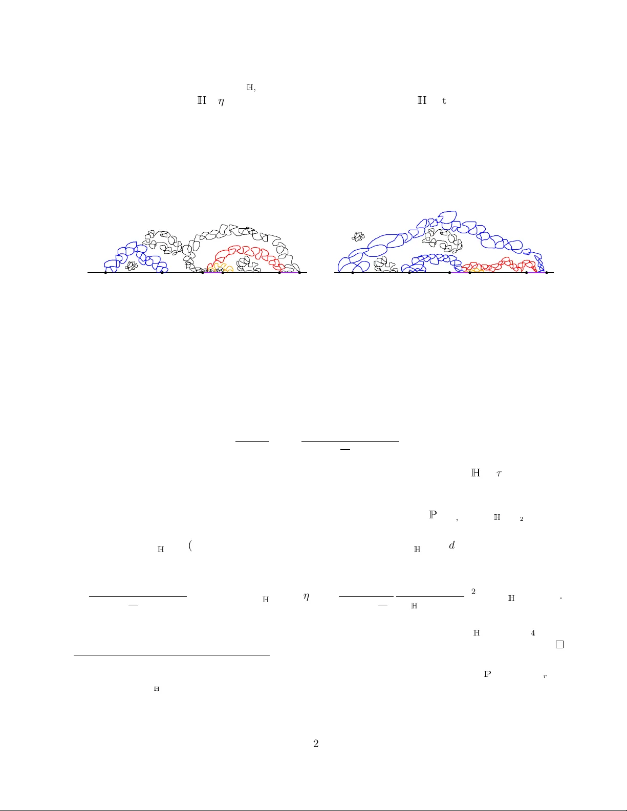
Boundary four-p oin t connectivities of conformal lo op ensem bles Gefei Cai ∗ Marc h 31, 2026 Abstract W e derive the b oundary four-point Green’s functions for conformal lo op ensembles (CLE) with κ ∈ (4 , 8). Specializing to κ = 6 and κ = 16 / 3, w e establish the exact form ulas for the b oundary four-p oin t connectivities in critical Bernoulli p ercolation and the FK-Ising mo del conjectured by Gori-Viti (2017, 2018). In particular, w e identify a logarithmic singularit y in the critical FK- Ising mo del. Our approach also applies to the one-bulk and tw o-b oundary connectivities of CLE, thereb y extending the factorization formula of Beliaev-Izyuro v (2012) to all κ ∈ (4 , 8). Con ten ts 1 In tro duction 1 2 SLE bubble measures and CLE b oundary Green’s functions 8 3 F usion 15 4 Iden tiﬁcation of solutions 17 5 One-Bulk and tw o-b oundary connectivities 26 A Boundary Green’s functions of SLE 28 B Discrete conv ergence 32 C MA TLAB co de 33 1 In tro duction F or ov er tw o decades, Sc hramm–Lo ewner ev olution (SLE) [Sch00] and its lo op coun terpart, the con- formal lo op ensem ble (CLE) [She09, SW12], hav e pla y ed a central role in the study of scaling limits of t wo-dimensional critical models. The family SLE κ , indexed by κ > 0, describ es random fractal curv es that arise as scaling limits of interfaces in critical lattice mo dels, while CLE κ describ es collections of lo ops that enco de their full scaling limits, with eac h lo op lo cally b ehaving like an SLE κ . In this pap er, we fo cus on the regime κ ∈ (4 , 8), which is conjectured to describ e the scaling limits of critical FK- q p ercolation mo dels with q ∈ (0 , 4), where √ q = − 2 cos(4 π /κ ). F or Bernoulli p ercolation ( q = 1), Smirno v’s seminal w ork [Smi01] established conformal in v ariance and con vergence to SLE 6 [Smi01, CN07], and to CLE 6 for the full scaling limit [CN06]. F or the FK-Ising model ( q = 2), the scaling limit has also b een pro ved to b e CLE 16 / 3 [CDCH + 14, KS19, KS16]. ∗ caigefei1917@pku.edu.cn , Peking Universit y . 1 Bey ond scaling limits, SLE and CLE pro vide p o w erful to ols for unco vering the rich integrable structures in critical planar lattice mo dels, and man y results that once app eared m ysterious at the discrete lev el can no w b e established through SLE/CLE. Notable examples include p ercolation arm exp onen ts [SW01, LSW02], left-passage probabilities [Sc h01], W atts’ crossing form ula [Dub06b], and conformal radii of CLE [SSW09]. Suc h in tegrable structures also emerge in the study of m ultiple SLEs and systems of second-order Bela vin–P olyak o v–Zamolo dc hiko v (BPZ) equations [BPZ84], which yield connection probabilities for multiple interfaces in v arious critical mo dels; see e.g. [PW19, LPW25, FPW24, FLPW24]. Exact solv abilities for SLE/CLE ha v e also b een obtained through their cou- pling with Liouville quantum gravit y (LQG) [DMS21, AHS24], including deriv ations of the bac kb one exp onen t [NQSZ24] and three-p oin t connectivity [ACSW24] in critical p ercolation. While t wo- and three-p oint observ ables are no w well understoo d [ACSW24], four-p oin t connec- tivities exhibit nontrivial dep endence on the conformal cross-ratio. In this pap er, we deriv e b oundary four-p oin t connectivities for CLE κ with κ ∈ (4 , 8). These quantities are the (conjectural) scaling lim- its of the probabilities that four marked b oundary p oin ts are connected according to one of the three p ossible link patterns { (1234) , (12)(34) , (14)(23) } in critical FK- q p ercolation with free b oundary con- ditions; see (1.1) and (1.3) for precise deﬁnitions. F or special v alues of κ corresp onding to integer q , explicit form ulas were previously conjectured by Gori and Viti [GV17, GV18] from a conformal ﬁeld theory (CFT) p erspective. In the four-p oin t setting, conformal automorphisms cannot ﬁx all marked p oin ts simultaneously , so the techniques from SLE/LQG coupling used in the three-point case [ACSW24] no longer apply . Moreo ver, since our problem concerns b oundary connectivities in CLE rather than conﬁgurations in volving m ultiple in terfaces, the metho ds of m ultiple SLE and BPZ equations developed in [PW19] are not directly applicable. Our approac h pro ceeds in four steps. First, we express th e CLE b oundary four-p oin t connectivities in terms of b oundary Green’s functions of the SLE bubble measure. Second, w e prov e that the b oundary Green’s functions of c hordal SLE satisfy a second-order BPZ equation, as exp ected in [FZ23]. Since the SLE bubble measure arises as a limit of chordal SLE, its b oundary Green’s functions are limits of solutions to this equation. Third, w e apply Dub´ edat’s fusion frame- w ork [Dub15a] to derive a third-order diﬀerential equation satisﬁed by these limiting ob jects, namely the four-p oin t connectivities; see Theorem 1.3. This framework, originating in CFT to pro duce higher-order BPZ equations, was rigorously form ulated in [Dub15a] in the SLE setting using PDE and represen tation-theoretic metho ds. Finally , for each link pattern, w e identify the corresp onding solution to this third-order equation. The ﬁnal step constitutes the main technical no velt y of the pap er; see Theorem 1.4. The third- order diﬀerential equation admits a three-dimensional space of solutions, corresponding to three distinct F rob enius series. F or the link patterns (12)(34) (resp. (14)(23)), the leading-order asymptotics as the cross-ratio tends to 1 (resp. 0) are go verned by b oundary three-arm exp onents, and th us allow for direct iden tiﬁcations with the higher-order F rob enius series. F or the remaining link pattern (1234), ho wev er, the leading order corresponds to the lo w est-order F rob enius series, and it is not a priori clear whether and how the other tw o F rob enius series may app ear as subleading terms. T o resolve this am biguity , we carry out a reﬁned analysis of the subleading asymptotics, based on the observ ation that the subleading term of the CLE partition function deﬁned in [MW18] with tw o wired b oundary arcs deca ys rapidly . This enables us to determine the higher-order contributions and to uniquely iden tify each b oundary connectivity with a sp eciﬁc solution to the third-order equation. W e ﬁrst presen t our results in the setting of critical p ercolation, conﬁrming the conjectural form ula in [GV18]. W e then extend the results to general CLE κ with κ ∈ (4 , 8) in Section 1.2. In particular, for κ = 16 3 (corresp onding to the FK-Ising mo del), we iden tify a logarithmic singularity in the b oundary 2 four-p oin t connectivities, reﬂecting the underlying logarithmic CFT structure and conﬁrming the conjectures of [GV17]. In Section 1.3, we summarize the main ideas of the pro of and discuss further applications. In particular, our approach also applies to one-bulk and t wo-boundary correlation functions; in this setting, we extend the factorization formula of [KSZ06, BI12] for κ = 6 to all κ ∈ (4 , 8) (see Theorem 1.7). 1.1 Boundary four-p oin t connectivities of Bernoulli p ercolation Let δ T ∩ H b e the triangular lattice on the upp er half-plane with mesh size δ . F or ( x i ) 1 ≤ i ≤ 4 ∈ R , we sa y they are in counterclockwise order if there exists k ∈ { 1 , 2 , 3 , 4 } such that x k < x k +1 < x k +2 < x k +3 (w e deﬁne x i +4 := x i for 1 ≤ i ≤ 4). F or ( x i ) 1 ≤ i ≤ 4 in counterclockwise order, let x δ i b e an appro ximation to x i on δ T ∩ H . Consider the critical Bernoulli p ercolation on δ T ∩ H , and denote its la w by P δ . Deﬁne the connectivities of the three distinct link patterns of ( x δ i ) 1 ≤ i ≤ 4 b y P (1234) ( x 1 , x 2 , x 3 , x 4 ) = lim δ → 0 δ − 4 3 P δ [ x δ 1 ↔ x δ 2 ↔ x δ 3 ↔ x δ 4 ] , P (12)(34) ( x 1 , x 2 , x 3 , x 4 ) = lim δ → 0 δ − 4 3 P δ [ x δ 1 ↔ x δ 2 ↔ x δ 3 ↔ x δ 4 ] , P (14)(23) ( x 1 , x 2 , x 3 , x 4 ) = lim δ → 0 δ − 4 3 P δ [ x δ 1 ↔ x δ 4 ↔ x δ 2 ↔ x δ 3 ] . (1.1) The existence of these limits is prov ed in [CF24, Theorem 1.9], and the normalization factor δ − 4 3 is from the p ercolation b oundary one-arm exp onen t 1 3 . Note that when ( x i ) 1 ≤ i ≤ 4 is in coun terclo c kwise order, one cannot hav e { x δ 1 ↔ x δ 3 ↔ x δ 2 ↔ x δ 4 } . W e also let P total ( x 1 , x 2 , x 3 , x 4 ) := P (1234) ( x 1 , x 2 , x 3 , x 4 ) + P (12)(34) ( x 1 , x 2 , x 3 , x 4 ) + P (14)(23) ( x 1 , x 2 , x 3 , x 4 ) . Our ﬁrst main res ult, Theorem 1.1, gives exact expressions for these limits, thereby proving the form ulas conjectured in [GV18]. Let ( x i ) 1 ≤ i ≤ 4 b e as ab ov e, and λ := ( x 2 − x 1 )( x 4 − x 3 ) ( x 4 − x 2 )( x 3 − x 1 ) ∈ (0 , 1) b e the cross-ratio of ( x i ) 1 ≤ i ≤ 4 . Deﬁne tw o functions F L ( λ ) = ( λ (1 − λ )) 4 9 3 F 2  − 2 9 , − 1 18 , 7 9 ; 1 3 , 2 3 ; 4 27 ( λ 2 − λ + 1) 3 (1 − λ ) 2 λ 2  , F S ( λ ) = (1 − λ ) 2 λ 2 3 F 2  4 3 , 3 2 , 7 3 ; 8 3 , 3; 4 λ (1 − λ )  . Here 3 F 2 is the generalized hypergeometric function. F or 0 < λ ≤ 1 2 , let V 2 ( λ ) := F S ( λ ), and there exist t wo real-v alued functions V 0 ( λ ) , V 1 / 3 ( λ ) suc h that F L ( λ ) = − e 2 πi 9 8 π 3 2 2 5 9 sin  4 π 9  3 5 6 Γ  5 6  Γ  − 1 18  2 Γ  7 9  V 0 ( λ ) + e πi 18 8 Γ  5 6  2 2 1 9 3 1 3 π 9 Γ  7 18  Γ  13 18  Γ  7 9  2 V 1 / 3 ( λ ) . Then we hav e V 0 ( λ ) = 1 − 2 3 λ + 8 45 λ 2 | log λ | + O ( λ 2 ), V 1 / 3 ( λ ) = λ 1 3 (1 − 1 2 λ + O ( λ 2 )), and V 2 ( λ ) = 3 λ 2 (1 + 1 3 λ + O ( λ 2 )) as λ ↓ 0. F or λ ∈ ( 1 2 , 1), w e deﬁne V 0 ( λ ) = V 0 (1 − λ ) , V 2 ( λ ) = α Im F L (1 − λ ) + F S (1 − λ ) with α := 405 64 π − 7 2 Γ  7 9  2 Γ  − 1 18  Γ  2 3  3 2 8 9 . Then V 0 , V 2 are smo oth real-v alued functions on (0 , 1). W e refer readers to [GV18, App endix C] for further details of these functions. Theorem 1.1. L et V 0 , V 2 b e deﬁne d as ab ove. Ther e exists a c onstant C ∈ (0 , ∞ ) such that P total ( x 1 , x 2 , x 3 , x 4 ) = C  ( x 4 − x 2 )( x 3 − x 1 ) ( x 2 − x 1 )( x 4 − x 3 )( x 3 − x 2 )( x 4 − x 1 )  2 3 V 0 ( λ ) , P (14)(23) ( x 1 , x 2 , x 3 , x 4 ) = AC  ( x 4 − x 2 )( x 3 − x 1 ) ( x 2 − x 1 )( x 4 − x 3 )( x 3 − x 2 )( x 4 − x 1 )  2 3 V 2 ( λ ) . Her e, the c onstant A := 8 √ 3 π sin ( 2 π 9 ) 135 cos ( 5 π 18 ) ∈ (0 , ∞ ) . By symmetry , we hav e P (12)(34) ( x 1 , x 2 , x 3 , x 4 ) = P (14)(23) ( x 4 , x 1 , x 2 , x 3 ). Thus, Theorem 1.1 also implies P (12)(34) ( x 1 , x 2 , x 3 , x 4 ) = AC  ( x 4 − x 2 )( x 3 − x 1 ) ( x 2 − x 1 )( x 4 − x 3 )( x 3 − x 2 )( x 4 − x 1 )  2 3 V 2 (1 − λ ). Consequen tly , Theo- rem 1.1 giv es the exact forms of the three limits in (1.1). F urthermore, when expanding at x 2 → x 1 (with x 1 , x 3 , x 4 ﬁxed; hence λ → 0), we hav e P total ( x 1 , x 2 , x 3 , x 4 ) = C ( x 2 − x 1 ) − 2 3 ( x 4 − x 3 ) − 2 3  1 + λ 2  8 45 | log λ | + 16 25  + O ( λ 3 | log λ | )  . Therefore, the universal constant C H 2 in [CF24, Theorem 1.9] equals 8 45 . As a corollary , w e ha ve the following exact form of the universal r atio P (14)(23) ( x 1 ,x 2 ,x 3 ,x 4 ) P total ( x 1 ,x 2 ,x 3 ,x 4 ) in tro duced in [GV18]. The term “universal” refers to the expectation that this ratio is indep enden t of the lattice. Corollary 1.2. L et ( x i ) 1 ≤ i ≤ 4 b e in c ounter clo ckwise or der, and λ = ( x 2 − x 1 )( x 4 − x 3 ) ( x 4 − x 2 )( x 3 − x 1 ) b e its cr oss-r atio. Then P (14)(23) ( x 1 , x 2 , x 3 , x 4 ) P total ( x 1 , x 2 , x 3 , x 4 ) = A V 2 ( λ ) V 0 ( λ ) = Aλ 2  1 + λ + λ 2  − 8 45 | log λ | + 1607 4950  + O ( λ 3 | log λ | )  as λ → 0 . Her e A is the same c onstant as in The or em 1.1. 1.2 Boundary four-p oin t connectivities of CLE W e now state our res ult for general CLE κ with κ ∈ (4 , 8), from which Theorem 1.1 follo ws b y taking κ = 6. CLE κ is a random collection of lo ops satisfying the domain Marko v prop erty and conformal in v ariance, and each lo op is an SLE κ curv e [She09, SW12]. When κ ∈ (4 , 8), CLE κ lo ops are self- touc hing and can touch eac h other. In the following, w e ﬁx κ ∈ (4 , 8) , h := 8 κ − 1 ∈ (0 , 1) . Let Γ b e a (non-nested) CLE κ on the upp er half-plane H , and let T (Γ) b e the collection of lo ops in Γ that touc h the b oundary ∂ H = R . F or each lo op ℓ ∈ T (Γ), denote ν ℓ ∩ R to b e the (1 − h )-dimensional 4 Mink owski conten t measure of ℓ ∩ R , suc h that for an y op en in terv al J ⊂ R , ν ℓ ∩ R ( J ) := lim ε → 0 ε − h Leb R ( { x ∈ J : dist( x, ℓ ∩ R ) < ε } ) . (1.2) The existence of ν η ∩ R is prov ed by [La w15] (see also [Zha22]) and the lo cal absolute contin uit y b et w een CLE κ and SLE κ . F or ( x i ) 1 ≤ i ≤ 4 ∈ R in coun terclo c kwise order, similar to (1.1), we deﬁne three t yp es of b oundary four-p oin t Green’s functions of CLE κ as G (1234) ( x 1 , x 2 , x 3 , x 4 ) dx 1 dx 2 dx 3 dx 4 = E   X ℓ ∈T (Γ) 4 Y i =1 ν ℓ ∩ R ( dx i )   , G (12)(34) ( x 1 , x 2 , x 3 , x 4 ) dx 1 dx 2 dx 3 dx 4 = E   X ℓ,ℓ ′ ∈T (Γ) 1 ℓ  = ℓ ′ 2 Y i =1 ν ℓ ∩ R ( dx i ) 4 Y j =3 ν ℓ ′ ∩ R ( dx j )   , G (14)(23) ( x 1 , x 2 , x 3 , x 4 ) = G (12)(34) ( x 4 , x 1 , x 2 , x 3 ) . (1.3) Here the exp ectation E is with resp ect to the CLE κ conﬁguration Γ on H . W e also let G total ( x 1 , x 2 , x 3 , x 4 ) = G (1234) ( x 1 , x 2 , x 3 , x 4 ) + G (12)(34) ( x 1 , x 2 , x 3 , x 4 ) + G (14)(23) ( x 1 , x 2 , x 3 , x 4 ) . W e also refer to (1.3) as b oundary four-p oint connectivities of CLE κ since they are the counterparts of (1.1) in the critical FK- q p ercolation, whose scaling limit is conjectured to b e CLE κ with √ q = − 2 cos(4 π /κ ). Let P b e the collection of link patterns, i.e. P := { (1234) , (12)(34) , (14)(23) , total } . Note that these b oundary Green’s functions satisfy the conformal cov ariance G p ( x 1 , x 2 , x 3 , x 4 ) = 4 Y i =1 | ϕ ′ ( x i ) | h ! · G p ( ϕ ( x 1 ) , ϕ ( x 2 ) , ϕ ( x 3 ) , ϕ ( x 4 )) , p ∈ P for an y M¨ obius transformation ϕ on H . Therefore, for each p ∈ P , there exists a function U p : (0 , 1) → R + of the cross-ratio λ = ( x 2 − x 1 )( x 4 − x 3 ) ( x 4 − x 2 )( x 3 − x 1 ) ∈ (0 , 1) suc h that G p ( x 1 , x 2 , x 3 , x 4 ) =  ( x 4 − x 2 )( x 3 − x 1 ) ( x 2 − x 1 )( x 4 − x 3 )( x 3 − x 2 )( x 4 − x 1 )  2 h U p ( λ ) . (1.4) Note that by symmetry , w e hav e U (14)(23) ( λ ) = U (12)(34) (1 − λ ). The follo wing result gives the diﬀeren tial equation satisﬁed by U p . Theorem 1.3. F or κ ∈ (4 , 8) and p ∈ P , U p ( λ ) is smo oth and solves the fol lowing thir d-or der ODE 1 2 κ 3 λ 2 (1 − λ ) 2 U ′′′ + κ 2 λ (3 κ − 16)(1 − λ )(1 − 2 λ ) U ′′ + κ  3( κ − 4)( κ − 8) + λ ( λ − 1)(18 κ 2 − 212 κ + 608)  U ′ + 6(2 λ − 1)( κ − 4)( κ − 8) 2 U = 0 . (1.5) 5 Note that the third-order ODE (1.5) also appeared in [GV18, Eq.(3.8)], where the CLE κ b oundary Green’s functions (1.3) are interpreted from the CFT p ersp ectiv e as correlation functions of the primary ﬁeld ϕ 1 , 3 with a level-three null vector. F or κ ∈ (4 , 8), no closed-form solutions of (1.5) are known in general. Note that 0 is a regular singular p oin t of (1.5), with indicial ro ots 0 , h, 3 h + 1. Then, in a neighborho o d of 0, we can use the F robenius metho d to ﬁnd three linearly indep enden t solutions V 0 , V h , V 3 h +1 of (1.5) suc h that V 0 ( λ ) = 1 + O ( λ ) , V h ( λ ) = λ h (1 + O ( λ )) , V 3 h +1 ( λ ) = λ 3 h +1 (1 + O ( λ )) . (1.6) Since (1.5) only has t wo singular points 0 and 1, we kno w that the three F robenius series V 0 , V h , V 3 h +1 con verge for all λ ∈ (0 , 1). When h and 3 h + 1 are both non-in tegers, the expressions 1 + O ( λ ) ab o v e are indeed p o wer series of λ . When h or 3 h + 1 is in teger (for κ ∈ (4 , 8),this only o ccurs when κ = 6 , 16 3 , 24 5 ), there might b e logarithmic terms in O ( λ ), and we ﬁnd explicit solutions in these cases separately . W e refer readers to [Inc44, Chapter XVI] for more bac kground on the F robenius metho d. The next theorem sho ws that the three t yp es of b oundary Green’s functions (1.3) can b e uniquely expressed in terms of the three linearly indep enden t solutions V 0 , V h , V 3 h +1 (1.6) of (1.5). Theorem 1.4. Ther e exist c onstants C 1 , C 2 ∈ (0 , ∞ ) such that for λ ∈ (0 , 1) , U (14)(23) ( λ ) = C 1 V 3 h +1 ( λ ) , U (12)(34) ( λ ) = U (14)(23) (1 − λ ) = C 1 V 3 h +1 (1 − λ ) , and U total ( λ ) = C 2 ( V 0 ( λ ) + β V 3 h +1 ( λ )) . Her e β ∈ R is the unique value with V 0 (1 − λ ) + β V 3 h +1 (1 − λ ) − 1 = o ( λ h ) , and the r atio C 1 C 2 is determine d by C 1 C 2 V 3 h +1 (1 − λ ) → 1 as λ → 0 . As we ha ve emphasized b efore, establishing U total ( λ ) = 1 + o ( λ h ) as λ → 0 requires a delicate analysis of b oundary G reen’s functions (1.3); see also the discussions in Section 1.3. F or κ = 6 and h = 1 3 , the functions V 0 , V 1 / 3 , V 2 in tro duced in Section 1.1 exactly correspond to the three solutions (1.6). Using a basic one-arm coupling in [Con15], one can show that the connectivities deﬁned in (1.1) agree with the CLE 6 b oundary four-p oin t Green’s functions in (1.3); see App endix B for details. Theorem 1.1 is then the κ = 6 case of Theorem 1.3 and 1.4. As another sp ecial case, taking κ = 16 3 giv es the b oundary four-p oin t connectivities of the critical FK-Ising mo del. Consider the critical FK-Ising mo del on δ Z 2 ∩ H with free b oundary condition. In analogy with the Bernoulli p ercolation, the limit P (1234) FK ( x 1 , x 2 , x 3 , x 4 ) = lim δ → 0 δ − 2 P δ FK [ x δ 1 ↔ x δ 2 ↔ x δ 3 ↔ x δ 4 ] exists [CF25, Theorem 1.4], and agrees with the CLE 16 / 3 b oundary four-p oin t Green’s function (see also App endix B). F or other p ∈ P , P p FK ( x 1 , x 2 , x 3 , x 4 ) is deﬁned similarly . By solving (1.5) with κ = 16 3 , these connectivities are explicit; see Section 4.2. In particular, w e hav e Theorem 1.5. L et R FK ( λ ) = P (12)(34) FK ( x 1 ,x 2 ,x 3 ,x 4 ) P total FK ( x 1 ,x 2 ,x 3 ,x 4 ) , and for x ∈ (0 , 1) , deﬁne g ( x ) = − (1 − x ) 3 / 2  (2 − 4 x ) 2 F 1  3 2 , 7 2 ; 3; 1 − x  − 3 x (1 − x ) 2 F 1  5 2 , 9 2 ; 4; 1 − x  x 3 / 2 2 ( x + (1 − x ) 2 ) 2 . (1.7) Then we have R FK ( λ ) = A FK R λ 0 g ( x ) dx , with A FK = ( R 1 0 g ( x ) dx ) − 1 ≈ 1 . 19948 . Theorem 1.5 prov es the conjectural form ula in [GV17, Eq.(6)]. Remark ably , taking λ = 1 − ε with ε → 0 (i.e. x 2 → x 3 with x 1 , x 3 , x 4 ﬁxed), w e hav e R FK (1 − ε ) = 1 − A FK ε 1 2  64 21 π + 16 21 π ε − 941 − 840 log 2 − 210 | log ε | 525 π ε 2 + O  ε 3 | log ε |   . 6 See also [GV17, Eq.(S12)]. T o our knowledge, this provides the ﬁrst rigorous evidence that a loga- rithmic singularit y app ears in the correlation functions of the critical FK-Ising mo del. Remark 1.6. In [FLPW24, Conje ctur e 1.2], the authors formulate a pr e cise c onje ctur e for the lim- iting c onne ction pr ob abilities of gener al critic al lo op O ( n ) mo dels, which also give the c onje ctur al c onne ction pr ob abilities for multichor dal CLE κ with 2 N b oundary ar cs (se e [AMY25]). In the r e gime κ ∈ (4 , 8) , this c onje ctur e was pr ove d for n = √ 2 (FK-Ising) [FPW24] and for 2 N = 4 [MW18]. In principle, by taking 2 N = 8 and shrinking four of the eight b oundary ar cs, one c ould obtain the CLE b oundary Gr e en ’s functions (1.3) via r enormalize d limits of the c orr esp onding c onje ctur al c on- ne ction pr ob abilities. However, this do es not se em pr actic al ly fe asible, sinc e the explicit formulas for these c onje ctur al c onne ction pr ob abilities involve the pur e p artition functions, whose c onstructions ar e highly nontrivial [FK15, KP16, Wu20, Zha24, FLPW24]. It is ther efor e uncle ar whether our r esults c an b e r e c over e d in this way fr om these c onje ctur al formulas. 1.3 Discussions W e no w brieﬂy discuss our pro of strategy . The ﬁrst step is to iden tify a precise corresp ondence b et w een CLE κ and the SLE κ bubble measure for κ ∈ (4 , 8). T o achiev e this, we show that the lo op sampled from the counting meas ure on b oundary-touc hing loops in a CLE κ conﬁguration is equal in law to the unro oted SLE κ bubble measure, see Prop osition 2.2. This identiﬁcation allows us to express the b oundary Green’s functions of CLE κ (1.3) in terms of those of the SLE κ bubble measure. F urthermore, SLE κ bubble measure is also the w eak limit of the chordal SLE κ when its starting p oin t approaches its end p oin t. According to [FZ23], the b oundary Green’s functions of c hordal SLE κ are ﬁnite and satisfy a martingale prop ert y as the chordal SLE κ gro ws. Com bined with their smo othness, the martingale prop ert y then yields a pair of second-order PDEs, kno wn as BPZ equations. Establishing suc h smo othness is non trivial and relies on H¨ ormander’s h yp o ellipticit y; see Lemma 2.8, as inspired b y [Dub15b, FZ23]. Then, w e apply a fusion pro cedure to these PDEs to deriv e a third-order diﬀerential equation satisﬁed by b oundary Green’s functions of the SLE κ bubble, whic h corresp onds to collapsing tw o mark ed b oundary p oin ts. As mentioned b efore, this step follows from the framew ork in [Dub15a], which also app eared in recent works [KLPR25, LPR25] for sp eciﬁc v alues of κ . This pro ves Theorem 1.3. Theorem 1.4 requires a delicate asymptotic analysis for the b oundary Green’s functions deﬁned in (1.3). Its crucial ingredien t is Prop osition 4.1, which establishes the o ( λ h ) subleading order in the sum of the Green’s functions G (1234) ( x 1 , x 2 , x 3 , x 4 ) + G (12)(34) ( x 1 , x 2 , x 3 , x 4 ) as the cross-ratio λ → 0. The pro of of Prop osition 4.1 is arguably the most subtle part of this pap er. In particular, it in volv es re-expressing the Green’s functions via a careful decomp osition of b oundary-touc hing CLE κ lo ops (see Corollary 4.6), as well as noting the rapid subleading decay in the partition function of CLE κ with tw o wired b oundary arcs, based on its connection probabilit y [MW18] (see (4.11)). According to [FLPW24, Lemma 6.1], such rapid decay of subleading terms also holds for Coulom b gas in tegrals, whic h are conjectured to b e the partition functions of general multic hordal CLE κ . Theorems 1.1 and 1.5 then follow by taking κ = 6 and κ = 16 3 . Our approach to the b oundary four-p oint Green’s functions can b e extended to the one-bulk and t wo-boundary connectivities of CLE κ . Let x 1 , x 2 ∈ R , z ∈ H , and consider the Green’s function G ( x 1 , x 2 , z ) dx 1 dx 2 dz = E   X ℓ ∈T (Γ) Υ ℓ ( dz ) 2 Y i =1 ν ℓ ∩ R ( dx i )   . (1.8) 7 Here, Υ ℓ denotes the Mil ler-Schoug me asur e [MS24] of the CLE κ gask et surrounded by ℓ . The Miller- Sc houg measure is a canonical measure supp orted on the CLE κ gask et, characterized by conformal co v ariance and the domain Mark ov prop ert y . It is conjectured to coincide with the (2 − α )-dimensional Mink owski conten t of the CLE κ gask et, where α := (3 κ − 8)(8 − κ ) 32 κ . F or CLE 6 gask et, its Miller-Schoug measure is sho wn to b e the scaling limit of the normalized counting measure on the critical percolation cluster [GPS13, CL24]. Consequently , G ( x 1 , x 2 , z ) can b e interpreted as the normalized probabilit y that x 1 , x 2 , and z belong to the same cluster. Theorem 1.7. F or κ ∈ (4 , 8) , let h = 8 κ − 1 and α b e as ab ove. Then G ( x 1 , x 2 , z ) = C | x 2 − x 1 | − h Im( z ) h − α | z − x 1 | − h | z − x 2 | − h (1.9) for some c onstant C ∈ (0 , ∞ ) . F or the case of critical Bernoulli p ercolation (i.e. κ = 6), Theorem 1.7 reco v ers the factoriza- tion formula conjectured b y [KSZ06] and later prov ed by [BI12]: the square of the one-bulk and t wo-boundary connectivity at z ∈ H , x 1 , x 2 ∈ R factorizes as the pro duct of t wo bulk-b oundary con- nectivities at ( z , x 1 ) and ( z , x 2 ) and the b oundary tw o-p oin t connectivity at ( x 1 , x 2 ). Theorem 1.7 extends this remark ably simple structure to all κ ∈ (4 , 8), showing that the factorization is in fact a univ ersal feature of CLE κ and hence of critical FK- q p ercolation. Ho wev er, our approach do es not apply to the bulk t wo-point correlation functions, which were recen tly conjectured in ph ysics [DJNS26], as the to ols of the Lo ewner equation are no longer av ailable. The same limitation applies to the four-p oin t functions on the sphere. F or the latter, diﬀeren tial equations can b e derived from the CFT p erspective in some sp ecial cases [GC06], whic h admit exact closed-form solutions. It would be interesting to explore whether suc h equations admit a probabilistic in terpretation in the SLE con text. Organization of the pap er. Section 2 is devoted to expressing the CLE κ b oundary Green’s func- tions in terms of the SLE κ bubble measure, and showing that the latter are the corresp onding limits of c hordal SLE κ . Then in Section 3, w e prov e Theorem 1.3. In Section 4, w e prov e Theorem 1.4 (and hence Theorems 1.1 and 1.5). W e also include solutions to (1.5) for other sp ecial κ ’s in Section 4.3. In Section 5, we prov e Theorem 1.7. In App endix A, we provide a detailed bac kground on the deﬁni- tions of SLE b oundary Green’s functions. App endix B gives relev ant discrete details in the pro of of Theorems 1.1 and 1.5. W e also provide MA TLAB code in App endix C that veriﬁes the calculation of deriving (1.5) from Section 3. Ac kno wledgment. This work was supp orted by the National Natural Science F oundation of China (Gran t No. 12526204) and National Key R&D Program of China (No. 2021YF A1002700). 2 SLE bubble measures and CLE b oundary Green’s functions In the follo wing, we ﬁx κ ∈ (4 , 8) and h := 8 κ − 1 ∈ (0 , 1). F or a ﬁnite measure M , we denote its total mass by | M | , and denote M # := 1 | M | M . W e usually use the sup erscript # to indicate that some measure is a probability measure. F or a compact set A ⊂ H , we denote U ( A ) to b e the unbounded connected comp onen t of H \ A . F or z ∈ C and ε > 0, we let B ( z , ε ) := { w ∈ C : | w − z | < ε } . F or x ∈ R , w e also let I ( x, ε ) b e the op en interv al ( x − ε, x + ε ). W e ﬁrst review the background on the SLE bubble measure in Section 2.1, and then show the re- lation b et ween boundary-touching CLE lo ops and the (unro oted) SLE bubble measure in Section 2.2. 8 In Section 2.3, w e relate the CLE b oundary four-p oin t connectivities (1.3) to the b oundary Green’s functions of SLE bubble and of chordal SLE. In Section 2.4, we show the smo othness of these b ound- ary Green’s functions, th us obtaining a pair of second-order PDEs satisﬁed b y the b oundary Green’s functions of chordal SLE, which will b e the basis of the fusion pro cedure in Section 3. 2.1 SLE bubble measure The SLE κ bubble measure was ﬁrst in tro duced in [SW12], and systematically studied in [Zha25]. F or x, y ∈ R , let µ # H ,x,y b e the la w of the c hordal SLE κ from x to y . Then the SLE κ bubble measure µ Bub x ro oted at x is deﬁned b y the weak limit µ Bub x = lim ε → 0 ε − h µ # H ,x,x + ε . (2.1) F or γ sampled from µ Bub x , the (1 − h )-dimensional Mink owski conten t measure ν γ ∩ R of γ ∩ R ex- ists [Zha22, Theorem 6.17]. According to [Zha25, Theorem 4.8], we can deﬁne the SLE κ bubble measure µ Bub x,y with t wo marked points x, y such that µ Bub x,y ( dγ ) dy = ν γ ∩ R ( dy ) µ Bub x ( dγ ) . (2.2) Here the total mass of µ Bub x,y ( dγ ) is C | y − x | − 2 h , where C ∈ (0 , ∞ ) is a ﬁxed constant introduced in [Zha25, Eq.(58)]. Such µ Bub x and µ Bub x,y corresp onds to the one-p oin t and tw o-p oin t pinned loop measures in [SW12], resp ectiv ely . According to [Zha25, Section 4.2], for x < y , the normalized probabilit y measure ( µ Bub x,y ) # can b e decomp osed as follows: ﬁrst sample the chordal SLE κ (2) curv e η on H from x to y with force p oin t at x − , and then sample the chordal SLE κ curv e η ′ on the remaining un b ounded domain U ( η ) from y to x . Then the concatenation of η and η ′ has the same la w as ( µ Bub x,y ) # . The marginal law of η ′ is the chordal SLE κ (2) from y to x , with force p oin t at y − . F rom (2.1), we also in tro duce the unr o ote d SLE κ bubble measure µ Bub via µ Bub ( dγ ) = 1 | ν γ ∩ R | 2 Z R × R µ Bub x,y ( dγ ) dxdy . (2.3) By [Zha25, Theorem 4.13], µ Bub then is inv ariant under M¨ obius transforms on H , with ν γ ∩ R ( dx ) µ Bub ( dγ ) = µ Bub x ( dγ ) dx, (2.4) ν γ ∩ R ( dx ) ν γ ∩ R ( dy ) µ Bub ( dγ ) = µ Bub x,y ( dγ ) dxdy . (2.5) W e refer readers to [Zha25] for further background on SLE κ bubble measures. The follo wing result from [SW12] links CLE κ to the SLE κ bubble measure. The original statemen t in [SW12] is for simple CLE κ , i.e. κ ∈ ( 8 3 , 4]. How ever, since the pro of there only uses the conformal Mark ovian exploration pro cess of CLE κ , which is based on the domain Marko v prop ert y of CLE κ and conformal in v ariance, the result is still v alid for κ ∈ (4 , 8). Lemma 2.1 ([SW12]) . Supp ose z ∈ H , and Γ is a CLE κ on H . L et T ε ( z ) (r esp. b T ε ( z ) ) b e the event that the CLE κ lo op surr ounding z interse cts B (0 , ε ) (r esp. I (0 , ε ) ). Then as ε → 0 , b oth P [ T ε ( z )] and P [ b T ε ( z )] ar e ε h + o (1) ; c onditione d on T ε ( z ) (r esp. b T ε ( z ) ), the c onditional law of ℓ c onver ges to µ Bub 0 c onditione d to surr ound z . 9 2.2 Boundary-touc hing CLE lo ops and unro oted SLE bubble measure W e now relate the b oundary-touc hing CLE κ lo ops to the unro oted SLE κ bubble measure. Prop osition 2.2. L et Γ b e a CLE κ c onﬁgur ation on H , and let T (Γ) b e the c ol le ction of lo ops in Γ that touch R . Denote ρ to b e the law of the outer b oundary of the lo op chosen fr om the c ounting me asur e, i.e. ρ ( A ) = E h P ℓ ∈T (Γ) 1 ℓ ∈A i for any me asur able A . Then ther e exists C ∈ (0 , ∞ ) such that ρ is e qual to the unr o ote d SLE κ bubble me asur e C µ Bub deﬁne d in (2.3) . Pr o of. Let ℓ z ∈ Γ b e the outermost lo op with its outer b oundary surrounding z ∈ H . W e claim that ℓ z , restricted on that ℓ z ∩ R  = ∅ , has the same la w as the unro oted SLE κ bubble measure µ Bub restricted on surrounding z . The result then follows b y v arying z . Denote the law of ℓ z b y Θ z . Let u ( ε ) = P [ b T ε ( i )] = ε h + o (1) where b T ε ( i ) is deﬁned in Lemma 2.1. F or x ∈ R and ε > 0, let E z ,x,ε b e the even t that ℓ z in tersects I ( x, ε ). No w, consider the measure M ε := u ( ε ) − 1 1 E z,x,ε Θ z ( dℓ ) dx . Note that for ﬁxed x ∈ R , Lemma 2.1 implies that the measure u ( ε ) − 1 1 E z,x,ε Θ z con verges weakly to C 1 F z,x µ Bub x as ε → 0, where F z ,x is the ev ent that the bubble ro oted at x surrounds z and C ∈ (0 , ∞ ) is some constant (throughout this pro of, C stands for some constant whose v alue can v ary from line to line). F urthermore, b y conformal co v ariance, the con vergence is uniform on an y b ounded in terv al U ⊂ R . Th us, we hav e the v ague con vergence M ε → M := C 1 F z,x µ Bub x ( dγ ) dx = C 1 γ surrounds z ν γ ∩ R ( dx ) µ Bub ( dγ ) (2.6) as ε → 0. Here the last equality is due to (2.4). On the other hand, note that for a.s. ℓ sampled from Θ z ( dℓ ) suc h that ℓ ∩ R  = ∅ , by [Zha22, Theorem 6.17], ε − h 1 E z,x,ε dx weakly conv erges to the (1 − h )-dimensional Mink owski conten t ν ℓ ∩ R of ℓ ∩ R . F urthermore, for an y bounded in terv al J ⊂ R , w e hav e ε − h R J 1 E z,x,ε dx → ν ℓ ∩ R ( J ) for Θ z -a.s. ℓ as w ell as in L 2 . Therefore, for an y compactly supp orted and contin uous function f , we ha ve ε − h Z 1 E z,x,ε f ( x, ℓ ) dx Θ z ( dℓ ) → Z f ( x, ℓ ) ν ℓ ∩ R ( dx )Θ z ( dℓ ) . Since R f ( x, ℓ ) M ε ( dx, dℓ ) = ε h u ( ε ) ε − h R 1 E z,x,ε f ( x, ℓ ) dx Θ z ( dℓ ), which con verges to R f ( x, ℓ ) M ( dx, dℓ ) b y (2.6), this implies the existence of the limit lim ε → 0 ε h u ( ε ) = C ∈ (0 , ∞ ). Consequen tly , Z f ( x, ℓ ) M ( dx, dℓ ) = C Z f ( x, ℓ ) ν ℓ ∩ R ( dx )Θ z ( dℓ ) , whic h gives the v ague conv ergence M ε → C 1 ℓ ∩ R  = ∅ ν ℓ ∩ R ( dx )Θ z ( dℓ ) (2.7) as ε → 0. Comparing (2.6) and (2.7), by deweigh ting the total masses of the b oundary Minko wski con tent measures, we obtain 1 γ surrounds z µ Bub ( dγ ) = C 1 ℓ ∩ R  = ∅ Θ z ( dℓ ). No w, since ρ is obtained from the counting measure on b oundary-touc hing lo ops and ev ery z ∈ H is surrounded by at most one CLE lo op, w e ha ve 1 ℓ surrounds z ρ ( dℓ ) dz = 1 ℓ ∩ R  = ∅ Θ z ( dℓ ) dz , where dz is the Leb esgue measure on H . Com bined with the ab o v e result, we ﬁnd 1 γ surrounds z µ Bub ( dγ ) dz = C 1 ℓ surrounds z ρ ( dℓ ) dz . The result then follows b y deweigh ting the Leb esgue areas of the regions surrounded b y the bubble (resp. lo op) on b oth sides. 10 According to Lemma A.3, the pro of of Prop osition 2.2 also works when we consider T ε instead of b T ε (and consider the even t that ℓ z in tersects B ( x, ε ) in the deﬁnition of E z ,x,ε ). As a byproduct of the pro of of Prop osition 2.2, we record the follo wing corollary . Corollary 2.3. L et T ε and b T ε b e as in L emma 2.1. Then b oth lim ε → 0 ε − h P [ T ε ] and lim ε → 0 ε − h P [ b T ε ] exist and ar e in (0 , ∞ ) . In p articular, the law of 1 T ε ℓ (or 1 b T ε ℓ ), times ε − h , c onver ges we akly to C µ Bub 0 r estricte d to surr ound z for some C ∈ (0 , ∞ ) . 2.3 CLE b oundary Green’s functions The aim of this section is to relate the CLE κ b oundary Green’s functions deﬁned in (1.3) to the limit of b oundary Green’s function of c hordal SLE κ ; see Prop osition 2.7. Due to symmetry , it suﬃces to fo cus on G (1234) ( x 1 , x 2 , x 3 , x 4 ) and G (12)(34) ( x 1 , x 2 , x 3 , x 4 ). W e refer readers to App endix A for further bac kground of SLE κ b oundary Green’s functions, including the v arious deﬁnitions app eared in the literature [Zha22, FZ23] and their equiv alence to the deﬁnition in this pap er. Based on Prop osition 2.2, w e can ﬁrst express the CLE κ b oundary Gree n’s functions using the SLE κ bubble measure. Supp ose x, x 1 , ..., x n ∈ R . Let G Bub x ( x 1 , ..., x n ) b e the b oundary Green’s function of SLE κ bubble ro oted at x , deﬁned b y G Bub x ( x 1 , ..., x n ) n Y i =1 dx i = µ Bub x " n Y i =1 ν γ ∩ R ( dx i ) # . (2.8) Then G Bub x ( x 1 , ..., x n ) is ﬁnite and lo cally b ounded; see Prop osition A.5. Let H H ( x 1 , x 2 ) ∝ 1 | x 1 − x 2 | 2 b e the b oundary Poisson k ernel on H . F or any simply connected domain D and a, b ∈ ∂ D , let f b e a conformal map from D to H , and deﬁne H D ( a, b ) = | f ′ ( a ) || f ′ ( b ) | H H ( f ( a ) , f ( b )) (when ∂ D is smo oth near a and b ). Prop osition 2.2 then implies the following Prop osition 2.4. L et C b e the same c onstant as in Pr op osition 2.2. Then for any n ≥ 2 , we have G Bub x 1 ( x 2 , ..., x n ) dx 1 dx 2 ...dx n = C E   X ℓ ∈T (Γ) n Y i =1 ν ℓ ∩ R ( dx i )   . (2.9) When n = 2 , G Bub x 1 ( x 2 ) = C H H ( x 1 , x 2 ) h (we cho ose the c onstant of H H ( x 1 , x 2 ) such that the c o eﬃcient is C ). In p articular, for the CLE κ b oundary Gr e en ’s functions deﬁne d in (1.3) , we have G (1234) ( x 1 , x 2 , x 3 , x 4 ) = C G Bub x 1 ( x 2 , x 3 , x 4 ) ∈ (0 , ∞ ) , (2.10) G (12)(34) ( x 1 , x 2 , x 3 , x 4 ) = C Z H U ( γ ) ( x 3 , x 4 ) h µ Bub x 1 ,x 2 ( dγ ) ∈ (0 , ∞ ) (2.11) wher e µ Bub x 1 ,x 2 is deﬁne d in (2.2) . R e c al l that U ( A ) denotes the unb ounde d c onne cte d c omp onent of H \ A for a c omp act subset A ⊂ H . Pr o of. (2.9) is a direct consequence of Prop osition 2.2 and (2.8), and (2.10) is the sp ecial case of (2.9) with n = 4. G Bub x 1 ( x 2 ) ∝ H H ( x 1 , x 2 ) h follo ws from the conformal cov ariance, and we choose the constan t of the b oundary Poisson kernel such that G Bub x 1 ( x 2 ) = C H H ( x 1 , x 2 ) h . This further implies H U ( γ ) ( x 3 , x 4 ) h = C E U ( γ ) h P ℓ ∈T (Γ) Q 4 i =3 ν ℓ ∩ R ( dx i ) i (here E U ( γ ) stands for taking exp ectations with 11 resp ect to the CLE κ on the domain U ( γ )). Then by (1.3), Proposition 2.2 and the domain Marko v prop ert y of CLE κ , w e obtain (2.11). W e now express the righ t sides of (2.10) and (2.11) as limits of b oundary Green’s function of c hordal SLE κ . T o this end, we start b y deﬁning tw o types of b oundary Green’s functions F (1) and F (2) of chordal SLE κ . Let y 1 , y 2 ∈ R ∪ {∞} , and let η b e a c hordal SLE κ on H from y 1 to y 2 (whose la w is denoted by µ # H ,y 1 ,y 2 ( dη )). Let ν η ∩ R ( dx ) b e the (1 − h )-dimensional Minko wski conten t of η ∩ R . F or x 1 , ..., x n ∈ R , deﬁne the b oundary n -p oin t Green’s function G H ,y 1 ,y 2 ( x 1 , ..., x n ) of η as G H ,y 1 ,y 2 ( x 1 , ..., x n ) n Y i =1 dx i = Z n Y i =1 ν η ∩ R ( dx i ) µ # H ,y 1 ,y 2 ( dη ) , (2.12) where the in tegration is tak en o ver µ # H ,y 1 ,y 2 ( dη ). (2.12) is equiv alent to the boundary Green’s function considered in [FZ23]; see Prop osition A.2. Deﬁnition 2.5. Supp ose x 1 < x 2 < x 3 and y 1 , y 2 ∈ R ∪ {∞} . Deﬁne F (1) , F (2) as fol lows. • L et F (1) ( y 1 , y 2 , x 1 , x 2 , x 3 ) := G H ,y 1 ,y 2 ( x 1 , x 2 , x 3 ) . • Denote ρ # H ,y 1 ,y 2 ,x 1 ( dη ) to b e the law of chor dal SLE κ ( κ − 8) on H fr om y 1 to y 2 with for c e p oint at x 1 , which c an b e viewe d as a chor dal SLE κ fr om y 1 to y 2 and c onditione d to hit x 1 . L et F (2) ( y 1 , y 2 , x 1 , x 2 , x 3 ) := G H ,y 1 ,y 2 ( x 1 ) Z H U ( η ) ( x 2 , x 3 ) h ρ # H ,y 1 ,y 2 ,x 1 ( dη ) . (2.13) Her e U ( η ) is the unb oune d c onne cte d c omp onent of H \ η , and H U ( η ) stands for the b oundary Poisson kernel on U ( η ) . When x 2 or x 3 is not in U ( η ) , we set H U ( η ) ( x 2 , x 3 ) := 0 . The follo wing lemma gives basic prop erties of F (1) and F (2) . Lemma 2.6. F or j = 1 , 2 , the functions F ( j ) ( y 1 , y 2 , x 1 , x 2 , x 3 ) ar e ﬁnite and lo c al ly b ounde d. F ur- thermor e, for η sample d fr om µ # H ,y 1 ,y 2 and p ar ameterize d by its half-plane c ap acity, let g t : H \ η t → H b e the c orr esp onding L o ewner map such that g t ( η t ) = W t . Then M ( j ) t ( y 1 , y 2 , x 1 , x 2 , x 3 ) := 3 Y i =1 | g ′ t ( x i ) | h ! · F ( j ) ( W t , g t ( y 2 ) , g t ( x 1 ) , g t ( x 2 ) , g t ( x 3 )) (2.14) is a c ontinuous lo c al martingale. Pr o of. F or F (1) , its ﬁniteness and lo cal b oundedness follo ws from [FZ23, Theorem 1] (see Prop osi- tion A.2 for the equiv alence of (2.12) and the Green’s function deﬁned in [FZ23]). Giv en this, the ﬁniteness and lo cal boundedness of F (2) readily follo ws from (2.13) and the monotonicit y of b oundary P oisson k ernel, i.e. H U η ( x 2 , x 3 ) ≤ H H ( x 2 , x 3 ). The local martingale prop ert y is the direct consequence of the domain Marko v prop ert y of the c hordal SLE κ and conformal cov ariance. The following prop osition gives that G (1234) ( x 1 , x 2 , x 3 , x 4 ) and G (12)(34) ( x 1 , x 2 , x 3 , x 4 ) can b e ob- tained as normalized limits of F (1) and F (2) . 12 Prop osition 2.7. L et u < x 1 < x 2 < x 3 . Then as y 1 , y 2 → u , we have C lim y 1 ,y 2 → u | y 2 − y 1 | − h F (1) ( y 1 , y 2 ; x 1 , x 2 , x 3 ) = G (1234) ( u, x 1 , x 2 , x 3 ) C lim y 1 ,y 2 → u | y 2 − y 1 | − h F (2) ( y 1 , y 2 ; x 1 , x 2 , x 3 ) = G (12)(34) ( u, x 1 , x 2 , x 3 ) . wher e C is the same c onstant in Pr op ositions 2.2 and 2.4. Pr o of. By Proposition A.6, we ha ve | y 2 − y 1 | − h G H ,y 1 ,y 2 ( x 1 , ..., x n ) → G Bub u ( x 1 , ..., x n ). Combined with (2.10) in Prop osition 2.4 and taking n = 3 gives the ﬁrst equation. F or the second equation, note that as y 1 , y 2 → u , the weak limit of ρ # H ,y 1 ,y 2 ,x 1 in (2.13) is the SLE κ bubble measure µ Bub u,x 1 ro oted at u and x 1 , normalized to b e a probabilit y measure ( µ Bub u,x 1 ) # . Th us, we ha ve C lim y 1 ,y 2 → u | y 2 − y 1 | − h F (2) ( y 1 , y 2 , x 1 , x 2 , x 3 ) = C G Bub u ( x 1 ) Z H U ( γ ) ( x 2 , x 3 ) h ( µ Bub u,x 1 ) # ( dγ ) = C Z H U ( γ ) ( x 2 , x 3 ) h µ Bub u,x 1 ( dγ ) , whic h equals G (12)(34) ( u, x 1 , x 2 , x 3 ) due to (2.11) in Prop osition 2.4. 2.4 Smo othness and second-order PDEs Based on the lo cal martingale prop ert y (2.14) in Lemma 2.6, we are able to derive a second-order PDE satisﬁed by F ( j ) for j = 1 , 2. Ho wev er, in order to apply Ito’s formula, we need to a priori kno w the smo othness of F ( j ) . Here w e use H¨ ormander’s hypo ellipticit y to obtain the smo othness, whic h is inspired b y the pro of of [Dub15b, Theorem 6] and [FZ23, Remark 4.3]. Lemma 2.8. F or j = 1 , 2 , the functions F ( j ) ( y 1 , y 2 , x 1 , x 2 , x 3 ) in Deﬁnition 2.5 ar e smo oth on { ( y 1 , y 2 , x 1 , x 2 , x 3 ) ∈ R 5 : x 1 < x 2 < x 3 and y 1 , y 2 < x 1 } . Pr o of. Let F ( j ) ( x 1 , x 2 , x 3 ) = F ( j ) (0 , ∞ , x 1 , x 2 , x 3 ) for simplicit y . By conformal co v ariance, it suﬃces to sho w the smo othness of F ( j ) ( x 1 , x 2 , x 3 ) on { ( x 1 , x 2 , x 3 ) ∈ R 3 + : x 1 < x 2 < x 3 } . F or 1 ≤ i ≤ 3, let I i b e an op en in terv al con taining x i , and U = I 1 × I 2 × I 3 ⊂ R 3 + . Deﬁne a second-order diﬀerential op erator L on C ∞ ( U ) ∩ C ( U ) by L = κ 2 X 2 + 2 Y − 2 h 3 X i =1 1 x 2 i , X = 3 X i =1 ∂ x i , Y = 3 X i =1 1 x i ∂ x i . (2.15) Note that the Lie brac kets [ X , Y ] = − P 3 i =1 1 x 2 i ∂ x i and [ X , [ X , Y ]] = 2 P 3 i =1 1 x 3 i ∂ x i . Since x i ’s are m utually diﬀerent on U , the Lie algebra generated b y X and Y has rank 3 on U . Thus, L satisﬁes the H¨ ormander’s condition 1 . By [Bon69, Theorem 5.2], we can then deﬁne a Poisson op erator P : C ( ∂ U ) → C ∞ ( U ) ∩ C ( U ) for L such that for any ω ∈ C ( ∂ U ), ( P ω ) | ∂ U = ω and L ( P ω ) = 0. Let φ t b e the Lo ewner map with driving function W t = √ κB t . By (2.14), w e know M ( j ) t ( x 1 , x 2 , x 3 ) := Q 3 i =1 | φ ′ ( x i ) | h F ( j ) ( x 1 , x 2 , x 3 ) is a con tinuous lo cal martingale. F or each t ≥ 0, let X t := ( g t ( x 1 ) − W t , g t ( x 2 ) − W t , g t ( x 3 ) − W t ), and let τ b e the ﬁrst hitting time of ∂ U for ( X t ). By optional stopping 1 i.e. for tw o v ector ﬁelds X and Y , X , Y and their iterated Lie brac kets [ X , Y ] , [ X , [ X , Y ]] etc. span the whole tangen t space at every p oin t. 13 theorem, M ( j ) 0 ( X 0 ) = E [ M ( j ) τ ( X 0 )]. On the other hand, note that L deﬁned in (2.15) is the inﬁnites- imal generator of ( X t ) with the killing rate 2 h X 2 t . Let N ( j ) := P ( M ( j ) 0 | ∂ U ) ∈ C ∞ ( U ) (th us L N ( j ) = 0). Applying Dynkin’s formu la to ( X t ) yields N ( j ) ( X 0 ) = E  e − R τ 0 2 h X 2 t dt N ( j ) ( X τ )  = E [ | φ ′ τ ( X 0 ) | h N ( j ) ( X τ )] . Since X τ ∈ ∂ U , w e also hav e E [ | φ ′ τ ( X 0 ) | h N ( j ) ( X τ )] = E [ | φ ′ τ ( X 0 ) | h M ( j ) 0 ( X τ )] = E [ M ( j ) τ ( X 0 )] = M ( j ) 0 ( X 0 ) = F ( j ) ( X 0 ) . Therefore, F ( j ) = N ( j ) 0 ∈ C ∞ ( U ). The result then follows from v arying U . No w we are able to deriv e the second-order PDEs satisﬁed b y F ( j ) . Prop osition 2.9. L et u = 1 2 ( y 1 + y 2 ) and v = 1 2 ( y 2 − y 1 ) . Then for j = 1 , 2 , F ( j ) ( y 1 , y 2 , x 1 , x 2 , x 3 ) satisﬁes the fol lowing p air of se c ond-or der PDEs: κ 4 ( ∂ uu + ∂ v v ) + 1 + κ − 6 2 v ∂ v + 3 X i =1  4( x i − u ) ∂ x i ( x i − u ) 2 − v 2 − 2 h ( x i − u + v ) 2 − 2 h ( x i − u − v ) 2  ! F = 0 , κ 2 ∂ uv − 1 − κ − 6 2 v ∂ u + 3 X i =1  4 v ∂ x i ( x i − u ) 2 − v 2 + 2 h ( x i − u + v ) 2 − 2 h ( x i − u − v ) 2  ! F = 0 . (2.16) Pr o of. Let η b e parameterized b y its half-plane capacity , and let g t : H \ η t → H b e the corresponding Lo ewner map. According to SLE co ordinate c hange [SW05], ( η t ) can b e view ed as a chordal SLE κ ( κ − 6) on H from y 1 to ∞ , with force p oin t at y 2 . Th us, we ha ve ∂ t g t ( z ) = 2 g t ( z ) − W t , dW t = √ κdB t − κ − 6 g t ( y 2 ) − W t dt. By Lemma 2.6, M ( j ) t :=  Q 3 i =1 | g ′ t ( x i ) | h  · F ( j ) ( W t , g t ( y 2 ) , g t ( x 1 ) , g t ( x 2 ) , g t ( x 3 )) is a lo cal martingale. By Lemma 2.8, applying Ito’s formula to ( M ( j ) t ) giv es − 3 X i =1 2 h ( x i − y 1 ) 2 − κ − 6 y 2 − y 1 ∂ y 1 + 2 y 2 − y 1 ∂ y 2 + 3 X i =1 2 x i − y 1 ∂ x i + κ 2 ∂ 2 y 1 ! F ( j ) = 0 . This is also known as the second-order BPZ equation at y 1 . Let u = 1 2 ( y 1 + y 2 ) and v = 1 2 ( y 2 − y 1 ). Then equiv alen tly , − 3 X i =1 2 h ( x i − u + v ) 2 + 1 2 v  ( ∂ u + ∂ v ) − κ − 6 2 ( ∂ u − ∂ v )  + 3 X i =1 2 x i − u + v ∂ x i + κ 8 ( ∂ u − ∂ v ) 2 ! F ( j ) = 0 . (2.17) By reversibilit y , w e can also view η as a c hordal SLE κ from y 2 to y 1 (hence is equiv alent to a c hordal SLE κ ( κ − 6) from y 2 to ∞ with force p oint at y 1 ). Then similarly , (2.17) also holds with v replaced 14 b y − v . Namely , we hav e − 3 X i =1 2 h ( x i − u − v ) 2 − 1 2 v  ( ∂ u − ∂ v ) − κ − 6 2 ( ∂ u + ∂ v )  + 3 X i =1 2 x i − u − v ∂ x i + κ 8 ( ∂ u + ∂ v ) 2 ! F ( j ) = 0 . (2.18) Com bining (2.17) and (2.18) gives (2.16). 3 F usion F or j = 1 , 2, recall that Prop osition 2.7 establishes the conv ergence of v − h F ( j ) ( y 1 , y 2 , x 1 , x 2 , x 3 ) to G (1234) ( u, x 1 , x 2 , x 3 ) (or G (12)(34) ( u, x 1 , x 2 , x 3 )), as v := 1 2 ( y 2 − y 1 ) → 0 with u := 1 2 ( y 1 + y 2 ) ﬁxed. Moreo ver, Prop osition 2.9 gives the tw o second-order PDEs s atisﬁed by F ( j ) ( y 1 , y 2 , x 1 , x 2 , x 3 ). F ollowing the framework of [Dub15a], these ingredients will together imply that the limiting function G (1234) ( u, x 1 , x 2 , x 3 ) (or G (12)(34) ( u, x 1 , x 2 , x 3 )) satisﬁes a third-order diﬀerential equation. The aim of the current section is to derive this third-order equation, thereb y proving Theorem 1.3. W e will rely on the follo wing input from [Dub15a]. Lemma 3.1 ([Dub15a, Lemma 2]) . L et n ≥ 1 , x = ( x 1 , ..., x n ) and ε > 0 . L et U = { ( y 1 , y 2 , x ) : | y 1 − u | < ε, 0 ≤ y 2 − y 1 < ε, ∥ x − x 0 ∥ < ε } , and ∆ = { ( y 1 , y 2 , x ) ∈ U : y 1 = y 2 } . F or ρ, τ , σ ∈ R , c onsider the diﬀer ential op er ator M = 1 2 ∂ 2 y 1 +  ρ y 1 − y 2 + a ( y 1 , y 2 , x )  ∂ y 1 +  τ 2( y 2 − y 1 ) + b ( y 1 , y 2 , x )  ∂ y 2 + X +  − τ σ 2( y 1 − y 2 ) 2 + d ( y 1 , y 2 , x ) y 2 − y 1  (3.1) wher e X := P n i =1 c i ( y 1 , x ) ∂ x i , and a, b, c, d ar e smo oth on U . Supp ose α − < α + ar e the two r o ots of the indicial e quation α ( α − 1) + ( τ + 2 ρ ) α − τ σ = 0 . Supp ose f is a r e al-value d smo oth function on U \ ∆ such that M f = 0 and f = O (( y 2 − y 1 ) α − + δ ) for some δ > 0 . F urther, assume that for Y := ∂ y 1 and Y , X satisﬁes the H¨ ormander’s c ondition on U \ ∆ . Then ther e exists a smo oth function g on U such that f = ( y 2 − y 1 ) α + g . W e no w pro ve Theorem 1.3 based on Lemma 3.1, following the approach as explained in [Dub15a, Section 2]. By symmetry , w e will fo cus on the case u < x 1 < x 2 < x 3 . Pr o of of The or em 1.3. In (3.1), we take n = 3, ρ = κ − 6 κ , τ = 4 κ , σ = 0, a = b = 0, c i = 2 /κ x i − y 1 and d = − P 3 i =1 2 h/κ ( x i − y 1 ) 2 ( y 2 − y 1 ) (hence α − = 0, α + = h ). Then for j = 1 , 2, F ( j ) is smooth suc h that M F ( j ) = 0. F urthermore, by Prop osition 2.7, F ( j ) = O (( y 2 − y 1 ) h ) as y 2 → y 1 . By direct computation, w e hav e [ Y , X ] = P 3 i =1 2 /κ ( x i − y 1 ) 2 ∂ x i and [ Y , [ Y , X ]] = P 3 i =1 4 /κ ( x i − y 1 ) 3 ∂ x i , th us the H¨ ormander’s condition holds. Hence, we can apply Lemma 3.1 to F ( j ) to see that there exists a smo oth g ( j ) on U suc h that F ( j ) = v h g ( j ) ( u, v , x 1 , x 2 , x 3 ). Consider the T aylor expansion for g ( j ) = P N n ≥ 1 g ( j ) n v n + O ( v N +1 ) near v = 0, where each g ( j ) n is smo oth. Since F ( j ) is in v arian t under v ↔ − v , only ev en p o wers app ear, i.e. g ( j ) 2 n +1 = 0 for ev ery n ≥ 0. Consequen tly , F ( j ) has the expansion F ( j ) = v h N X n =0 v 2 n g ( j ) 2 n ( u, x 1 , x 2 , x 3 ) + O ( v 2 N +2 ) (3.2) 15 as v → 0. In particular, b y Prop osition 2.7, we hav e g (1) 0 ( u, x 1 , x 2 , x 3 ) = C G (1234) ( u, x 1 , x 2 , x 3 ) , g (2) 0 ( u, x 1 , x 2 , x 3 ) = C G (12)(34) ( u, x 1 , x 2 , x 3 ) (3.3) for some constant C ∈ (0 , ∞ ). The expansion for partial deriv ativ es of F ( j ) is similar, giving that ∂ u F ( j ) = v h N X n =0 v 2 n ∂ u g ( j ) 2 n ( u, x 1 , x 2 , x 3 ) + O ( v 2 N +2 ) , ∂ v F ( j ) = v h N X n =0 (2 n + h ) v 2 n − 1 g ( j ) 2 n ( u, x 1 , x 2 , x 3 ) + O ( v 2 N +1 ) (3.4) etc. (Note that h ∈ (0 , 1) is not an integer). T aking the ab ov e expansions (3.2), (3.4) into (2.16), b y comparing the co eﬃcien ts of v h − 2 and v h − 1 , w e ﬁrst obtain (the “zeroth order” equations) κ 4 h ( h − 1) +  1 + κ − 6 2  h = 0 , κ 2 h −  1 − κ − 6 2  = 0 , whic h b oth hold since h = 8 κ − 1. Iterativ ely , by comparing the co eﬃcien ts of v h and v h +1 , w e hav e (the “ﬁrst order” equations) κ 4  ∂ uu g ( j ) 0 + ( h + 2)( h + 1) g ( j ) 2  +  1 + κ − 6 2  ( h + 2) g ( j ) 2 + 3 X i =1 4 ∂ x i g ( j ) 0 x i − u − 4 hg ( j ) 0 ( x i − u ) 2 ! = 0 , κ 2 ( h + 2) ∂ u g ( j ) 2 −  1 − κ − 6 2  ∂ u g ( j ) 2 + 3 X i =1 4 ∂ x i g ( j ) 0 ( x i − u ) 2 − 8 hg ( j ) 0 ( x i − u ) 3 ! = 0 . Com bining the ab ov e tw o equations to eliminate g ( j ) 2 and taking into h = 8 κ − 1, w e obtain κ 4 ∂ 3 u g ( j ) 0 + 1 2  1 − 8 κ  3 X i =1 4 ∂ x i g ( j ) 0 ( x i − u ) 2 − 8 hg ( j ) 0 ( x i − u ) 3 ! + 3 X i =1 4 ∂ ux i g ( j ) 0 x i − u − 4 h∂ u g ( j ) 0 ( x i − u ) 2 ! = 0 . (3.5) Recall that by (3.3) and (1.4), for the cross-ratio λ = ( x 1 − u )( x 3 − x 2 ) ( x 3 − x 1 )( x 2 − u ) , w e hav e g (1) 0 ( u, x 1 , x 2 , x 3 ) = (1 − λ ) − 2 h U (1234) ( λ ) (( x 1 − u )( x 3 − x 2 )) 2 h , g (2) 0 ( u, x 1 , x 2 , x 3 ) = (1 − λ ) − 2 h U (12)(34) ( λ ) (( x 1 − u )( x 3 − x 2 )) 2 h (3.6) Substituting (3.6) into (3.5), (after a long but standard calculation; see App endix C for a veriﬁca- tion using MA TLAB) we obtain that U p ( λ ) satisﬁes (1.5) for p ∈ { (1234) , (12)(34) } . Finally , since U (14)(23) ( λ ) = U (12)(34) (1 − λ ) and (1.5) is in v arian t under λ ↔ 1 − λ , we hav e U (14)(23) ( λ ) also satisﬁes (1.5), so is U total ( λ ). 16 4 Iden tiﬁcation of solutions Recall that κ ∈ (4 , 8) and h = 8 κ − 1 ∈ (0 , 1). Theorem 1.4 is based on the following Prop osition 4.1. As x 2 → x 1 (with x 1 , x 3 , x 4 ﬁxe d), we have G (1234) ( x 1 , x 2 , x 3 , x 4 ) + G (12)(34) ( x 1 , x 2 , x 3 , x 4 ) = H H ( x 1 , x 2 ) h H H ( x 3 , x 4 ) h (1 + o ( | x 2 − x 1 | h )) . Pr o of of The or em 1.4, assuming Pr op osition 4.1. Let x 1 < x 2 < x 3 < x 4 . The iden tiﬁcation of U (14)(23) ( λ ) and U (12)(34) ( λ ) is straightforw ard. Indeed, b y (2.11) in Prop osition 2.4, w e hav e G (14)(23) ( x 1 , x 2 , x 3 , x 4 ) ∝ Z H U ( γ ) ( x 2 , x 3 ) h µ Bub x 4 ,x 1 ( dγ ) ≤ H H ( x 1 , x 4 ) h Z H U ( η ) ( x 2 , x 3 ) h µ # H ,x 4 ,x 1 ( dη ) = O ( | x 2 − x 1 | 4 κ ) , as x 2 → x 1 and x 1 , x 3 , x 4 ﬁxed . The inequalit y follows from that H U ( γ ) ( x 2 , x 3 ) under the la w of ( µ Bub x 4 ,x 1 ) # ( dγ ) is sto c hastically domi- nated by H U ( η ) ( x 2 , x 3 ) under µ # H ,x 4 ,x 1 ( dη ), according to the decomp osition of t wo-point ro oted SLE κ bubbles. The ﬁnal equality follo ws from [W u20, Lemma 3.4, Proposition 3.5] (with taking ν = 2 there; see also Lemma 4.3 b elo w). Therefore, U (14)(23) ( λ ) = O ( λ 12 κ − 1 ) = o ( λ h ) as λ → 0, and hence U (14)(23) ( λ ) = C 1 V 3 h +1 ( λ ) for some C 1 ∈ (0 , ∞ ). The identiﬁcation of U (12)(34) then follows from symmetry U (12)(34) ( λ ) = U (14)(23) (1 − λ ). The iden tiﬁcation of U total ( λ ) relies on Prop osition 4.1. Since U total ( λ ) is the solution of (1.5), th us there exists C 2 , α, β such that U total ( λ ) = C 2 ( V 0 ( λ ) + αV h ( λ ) + β V 3 h +1 ( λ )). By Prop osition 4.1, α = 0. On the other hand, since U total ( λ ) = U total (1 − λ ), Prop osition 4.1 also gives U total (1 − λ ) = C 2 (1 + o ( λ h )) as λ → 0. Note that U (1234) ( λ ) = O ( λ h ) as λ → 0 (this can b e seen e.g. b y com bining Prop osition 2.7 and the asymptotic b ehavior of the b oundary Green’s function of chordal SLE κ [FZ23, Theorem 1.1]). By Prop osition 4.1, we must ha ve U (12)(34) ( λ ) = C 2 + O ( λ h ) and hence V 3 h +1 (1 − λ ) = C 2 C 1 + O ( λ h ) as λ → 0. Th us suc h β is unique. The ratio C 1 C 2 is determined by U (12)(34) ( λ ) U total ( λ ) → 1 as λ → 0. In this section, we ﬁrst pro ve Prop osition 4.1 in Section 4.1, which relies on expressing G (1234) and G (12)(34) in terms of the partition function of CLE κ with tw o wired b oundary arcs [MW18] (see Corollary 4.6), and the explicit subleading b ehavior of the latter (4.11). Then in Section 4.2, w e pro ve Theorems 1.1 and 1.5 as applications of Theorems 1.3 and 1.4. As we mentioned b efore, in these cases, the explicit forms of V 0 , V h , V 3 h +1 w ere previously obtained in [GV17, GV18]. W e discuss solutions of (1.5) for other sp ecial κ ’s in Section 4.3. 4.1 Pro of of Prop osition 4.1 In this section we prov e Prop osition 4.1. W e ﬁx b = 6 − κ 2 κ throughout this section. Supp ose D is a Jordan domain, and x, y ∈ ∂ D . Let µ # D,x,y b e the law of c hordal SLE κ on D from x to y , and e µ # D,x,y b e the law of c hordal SLE κ (2) on D from x to y , with the force p oin t x − . When ∂ D is smo oth near x and y , w e denote µ D,x,y = H D ( x, y ) b µ # D,x,y and 17 e µ D,x,y = H D ( x, y ) h e µ # D,x,y . Note that e µ D,x,y is diﬀerent from e µ D,y ,x , while their total masses coincide. Here w e choose the constan t of the b oundary Poisson kernel as in Prop osition 2.4. W e start b y the follo wing forms of G (1234) ( x 1 , x 2 , x 3 , x 4 ) and G (12)(34) ( x 1 , x 2 , x 3 , x 4 ). According to symmetry , we fo cus on the case x 1 < x 2 < x 3 < x 4 throughout this section. Let G D,x 1 ,x 2 ( x 3 , x 4 ) b e the b oundary t w o-p oin t Green’s function of a c hordal SLE κ from x 1 to x 2 on D at ( x 3 , x 4 ) (when ∂ D is smo oth near x 3 , x 4 ) suc h that G D,x 1 ,x 2 ( x 3 , x 4 ) = | ϕ ′ ( x 3 ) ϕ ′ ( x 4 ) | h G H ,ϕ ( x 1 ) ,ϕ ( x 2 ) ( ϕ ( x 3 ) , ϕ ( x 4 )) for a conformal map ϕ : D → H , where G H ,ϕ ( x 1 ) ,ϕ ( x 2 ) ( ϕ ( x 3 ) , ϕ ( x 4 )) is deﬁned in (2.12). Lemma 4.2. We have G (1234) ( x 1 , x 2 , x 3 , x 4 ) = Z G U ( η 12 ) ,x 1 ,x 2 ( x 4 , x 3 ) e µ H ,x 1 ,x 2 ( dη 12 ) , (4.1) G (12)(34) ( x 1 , x 2 , x 3 , x 4 ) = Z H U ( η ′ ) ( x 3 , x 4 ) h µ # U ( η 12 ) ,x 1 ,x 2 ( dη ′ ) e µ H ,x 1 ,x 2 ( dη 12 ) . (4.2) Pr o of. (4.2) follo ws from (2.11) in Prop osition 2.4 and the decomposition of the SLE κ bubble measure with tw o mark ed p oin ts (see Section 2.1). F or (4.1), note that com bining Prop osition 2.2, (2.2) and the decomp osition ab ov e giv es E   X ℓ ∈T (Γ) 4 Y i =1 ν ℓ ∩ R ( dx i )   = Z ν η 12 ∩ R ( dx 3 ) ν η 12 ∩ R ( dx 4 ) µ # U ( η 12 ) ,x 1 ,x 2 ( dη ′ ) e µ H ,x 1 ,x 2 ( dη 12 ) dx 1 dx 2 . Here the integral on the right side is with resp ect to the measure e µ H ,x 1 ,x 2 ( dη 12 ). The result then follo ws from (2.12) and the conformal co v ariance of Minko wski con tent. W e pro ve Prop osition 4.1 by a detailed analysis of the righ t sides of (4.1) and (4.2). W e record the follo wing result from [W u20], which arises from the partition function of hypergeometric SLE 2 . Lemma 4.3 ([W u20, Lemma 3.4, Prop osition 3.5]) . F or η 12 sample d fr om µ H ,x 1 ,x 2 ( dη 12 ) , r e c al l that U ( η 12 ) is the unb ounde d c onne cte d c omp onent of H \ η 12 . F or ν ≥ κ 2 − 4 , let α = ν +2 κ and β = ( ν +2)( ν +6 − κ ) 4 κ . Then we have Z H U ( η 12 ) ( x 3 , x 4 ) β µ H ,x 1 ,x 2 ( dη 12 ) = H H ( x 1 , x 2 ) b H H ( x 3 , x 4 ) β (1 − λ ) α 2 F 1 (2 α, 1 − 4 κ ; 2 α + 4 κ ; 1 − λ ) 2 F 1 (2 α, 1 − 4 κ ; 2 α + 4 κ ; 1) , wher e λ = ( x 2 − x 1 )( x 4 − x 3 ) ( x 3 − x 1 )( x 4 − x 2 ) is the cr oss-r atio. W e mainly use the ν = 0 case of Lemma 4.3, which also app eared earlier in [BBK05, Dub06a]. In the follo wing, we write f ( x ) = x 2 κ (1 − x ) 1 − 6 κ 2 F 1 ( 4 κ , 1 − 4 κ ; 8 κ ; x ) 2 F 1 ( 4 κ , 1 − 4 κ ; 8 κ ; 1) . (4.3) 2 The term hypergeometric SLE was earlier introduced in [Qia18] to refer to a broader class of SLEs. 18 W e will rely on a key observ ation on the explicit subleading b eha vior of f ( x ) in the pro of of Prop o- sition 4.1; see (4.11) b elo w. The following lemma deals with the righ t side of (4.2). Lemma 4.4. Consider the me asur e e µ U ( η 12 ) ,x 3 ,x 4 ( dη 34 ) µ H ,x 1 ,x 2 ( dη 12 ) . Then its total mass Z H U ( η 12 ) ( x 3 , x 4 ) h µ H ,x 1 ,x 2 ( dη 12 ) = Z H U ( η ) ( x 1 , x 2 ) b τ 2 b f (1 − τ ) e µ H ,x 3 ,x 4 ( dη ) . (4.4) Her e τ ∈ (0 , 1) is such that the ( U ( η ) , x 1 , x 2 , x 3 , x 4 ) is c onformal ly e quivalent to ( H , 0 , τ , 1 , ∞ ) . Pr o of. The left side of (4.4) equals the total mass of e µ U ( η 12 ) ,x 4 ,x 3 ( dη 34 ) µ H ,x 1 ,x 2 ( dη 12 ). W e ﬁrst claim that it equals R H U ( η ′ ) ( x 1 , x 2 ) b e µ H ,x 4 ,x 3 ( dη ′ ) (i.e. the commutation relation of bi-chordal SLE κ and SLE κ (2) pair). Deﬁne M H ,x 3 ,x 4 ,ε := µ U ( η ′ ) ,x 3 ,x 4 ( dη 34 ) µ H ,x 3 − ε,x 4 + ε ( dη ′ ). By [W u20, Lemma 3.7], as ε → 0, the marginal la w of η 34 under M H ,x 3 ,x 4 ,ε (whic h corresp onds to the hypergeometric SLE with parameter ν = 0 there), times ε − 2 h , con verges w eakly to C e µ H ,x 4 ,x 3 ( dη 34 ) for some C ∈ (0 , ∞ ). No w consider the measure deﬁned on the triples N ε := µ U ( η 34 ) ,x 1 ,x 2 ( dη 12 ) M H ,x 3 ,x 4 ,ε ( dη 34 , dη ′ ). T aking ε → 0, the marginal la w of ( η 12 , η 34 ) under N ε th us con verges w eakly to C µ U ( η 34 ) ,x 1 ,x 2 ( dη 12 ) e µ H ,x 4 ,x 3 ( dη 34 ). On the other hand, using the symmetry for bi-c hordal SLE κ (see e.g. [W u20, Prop osition 6.10]) twice, w e also ha ve N ε = M U ( η 12 ) ,x 3 ,x 4 ,ε ( dη 34 , dη ′ ) µ H ,x 1 ,x 2 ( dη 12 ). Then as ε → 0, N ε also conv erges w eakly to C e µ U ( η 12 ) ,x 4 ,x 3 ( dη 34 ) µ H ,x 1 ,x 2 ( dη 12 ). Consequen tly , we hav e µ U ( η 34 ) ,x 1 ,x 2 ( dη 12 ) e µ H ,x 4 ,x 3 ( dη 34 ) = e µ U ( η 12 ) ,x 4 ,x 3 ( dη 34 ) µ H ,x 1 ,x 2 ( dη 12 ) , and the claim follows by comparing the total masses on b oth sides. Note that e µ H ,x 4 ,x 3 ( dη ′ ) can b e obtained b y ﬁrst sampling η from e µ H ,x 3 ,x 4 ( dη ), and then sampling η ′ from µ # U ( η ) ,x 3 ,x 4 . Com bined with the ab o v e claim, we hav e Z H U ( η 12 ) ( x 3 , x 4 ) h µ H ,x 1 ,x 2 ( dη 12 ) = Z H U ( η ′ ) ( x 1 , x 2 ) b µ # U ( η ) ,x 3 ,x 4 ( dη ′ ) e µ H ,x 3 ,x 4 ( dη ) . By Lemma 4.3 with ν = 0 (hence α = 2 κ and β = b ), the right side ab o ve equals Z H U ( η ) ( x 1 , x 2 ) b (1 − τ ) 2 κ 2 F 1 ( 4 κ , 1 − 4 κ ; 8 κ ; 1 − τ ) 2 F 1 ( 4 κ , 1 − 4 κ ; 8 κ ; 1) e µ H ,x 3 ,x 4 ( dη ) = Z H U ( η ) ( x 1 , x 2 ) b τ 2 b f (1 − τ ) e µ H ,x 3 ,x 4 ( dη ) , as desired. Next, w e use the connection probability of CLE κ with tw o wired b oundary arcs [MW18] to derive a similar expression for the b oundary tw o-p oin t Green’s function of chordal SLE κ , which deals with the right side of (4.1). W e refer readers to [MW18, Section 2] for backgrounds on CLE with tw o wired b oundary arcs. Recall the b oundary tw o-p oin t Green’s function G H ,x 1 ,x 2 ( x 3 , x 4 ) of the c hordal SLE κ deﬁned in (2.12). Lemma 4.5. We have H H ( x 1 , x 2 ) b G H ,x 1 ,x 2 ( x 3 , x 4 ) = 1 − 2 cos  4 π κ  Z H U ( η ) ( x 1 , x 2 ) b τ 2 b f ( τ ) e µ H ,x 3 ,x 4 ( dη ) . Her e τ is such that the ( U ( η ) , x 1 , x 2 , x 3 , x 4 ) is c onformal ly e quivalent to (0 , τ , 1 , ∞ ) . 19 Pr o of. Let η 12 b e sampled from µ # H ,x 1 ,x 2 , and Γ be sampled from an indep enden t CLE κ on each connected comp onen t of H \ η 12 . Then b Γ = Γ ∪ { η 12 } is a CLE κ on H with a wired b oundary arc [ x 1 , x 2 ]. F or i = 3 , 4 and r i > 0, let I ( x i , r i ) = ( x i − r i , x i + r i ). Denote E r 3 ,r 4 to b e the even t that there exists an element in b Γ that intersects b oth I ( x 3 , r 3 ) and I ( x 4 , r 4 ). On E r 3 ,r 4 , let ζ b e the CLE κ exploration interface of b Γ from x 3 + r 3 to x 3 − r 3 up to the ﬁrst time σ it hits I ( x 4 , r 4 ); see Figure 1. Let σ ′ b e the last time b efore σ that ζ hits I ( x 3 , r 3 ). Then conditioned on ζ [ σ ′ , σ ], the restriction of b Γ on U ( ζ [ σ ′ , σ ]) is a CLE κ on U ( ζ [ σ ′ , σ ]) with t wo wired boundary arcs: [ x 1 , x 2 ] and the outer b oundary of ζ [ σ ′ , σ ]. x 1 x 2 I ( x 3 , r 3 ) I ( x 4 , r 4 ) x 1 x 2 I ( x 3 , r 3 ) I ( x 4 , r 4 ) Figure 1: Illustration for the CLE κ exploration interface ζ of b Γ. The segmen t ζ [ σ, σ ′ ] is colored red, while ζ [0 , σ ′ ] is in orange. Left: the ev ent E r 3 ,r 4 \ F r 3 ,r 4 , and η 12 is colored blue. Right: the even t F r 3 ,r 4 , and η 12 is the union of the blue and red curves. Let F r 3 ,r 4 ⊂ E r 3 ,r 4 b e the even t that ζ [ σ ′ , σ ] ⊂ η 12 . Note that giv en E r 3 ,r 4 , whether F r 3 ,r 4 o ccurs or not giv es a dic hotomy of the tw o link patterns of b Γ. Let m r 3 ,r 4 (resp. m ′ r 3 ,r 4 ) b e the law of ζ [ σ ′ , σ ] restricted on F r 3 ,r 4 (resp. E r 3 ,r 4 \ F r 3 ,r 4 ). Then by [MW18, Theorem 1.1], m r 3 ,r 4 and m ′ r 3 ,r 4 are m utually absolutely contin uous, with the Radon-Nikodym deriv ativ e d m r 3 ,r 4 d m ′ r 3 ,r 4 ( η ) = f ( τ ) − 2 cos  4 π κ  f (1 − τ ) . (4.5) Here τ ∈ (0 , 1) is such that the ( U ( η ) , x 1 , x 2 , x 3 , x 4 ) is conformally equiv alen t to ( H , 0 , τ , 1 , ∞ ). On the other hand, note that F r 3 ,r 4 implies η 12 in tersecting b oth I ( x 3 , r 3 ) and I ( x 4 , r 4 ), while the in tersection of the latter ev ent and E r 3 ,r 4 \ F r 3 ,r 4 yields a boundary three-arm even t joining I ( x 3 , r 3 ) and I ( x 4 , r 4 ). Hence, by [Zha22, Theorem 5.1], w e ha ve lim r 3 ,r 4 → 0 r − h 3 r − h 4 P [ F r 3 ,r 4 ] = G H ,x 1 ,x 2 ( x 3 , x 4 ). F urthermore, according to Lemma A.7 and conformal cov ariance, r − h 3 r − h 4 m ′ r 3 ,r 4 w eakly conv erges to R µ U ( η 12 ) ,x 3 ,x 4 ( · ) µ # H ,x 1 ,x 2 ( dη 12 ) 3 (here the in tegration is tak en ov er µ # H ,x 1 ,x 2 ( dη 12 )) as r 3 → 0 then r 4 → 0. Com bined with (4.5), w e ﬁnd that r − h 3 r − h 4 m r 3 ,r 4 w eakly conv erges to the measure Z f ( τ ) − 2 cos  4 π κ  f (1 − τ ) µ U ( η 12 ) ,x 3 ,x 4 ( · ) µ # H ,x 1 ,x 2 ( dη 12 ) = 1 − 2 cos  4 π κ  H U ( η ) ( x 1 , x 2 ) b H H ( x 1 , x 2 ) b τ 2 b f ( τ ) e µ H ,x 3 ,x 4 ( dη ) . Here to the right side w e use Lemma 4.4. Combined with r − h 3 r − h 4 | m r 3 ,r 4 | → G H ,x 1 ,x 2 ( x 3 , x 4 ), the result then follows. 3 Here, using Lemma A.7 seems to inv olve some unspeciﬁed constant in the limiting measure. Ho wev er, such constan t is indeed ﬁxed according to Remark A.8: by conformal cov ariance, we hav e lim r 4 → 0 lim r 3 → 0 r − h 3 r − h 4 P [ E r 3 ,r 4 \ F r 3 ,r 4 ] = R H U ( η 12 ) ( x 3 , x 4 ) h µ # H ,x 1 ,x 2 ( dη 12 ). 20 By conformal cov ariance, for an y η 12 joining x 1 and x 2 , Lemmas 4.4 and 4.5 imply Z H U ( η ′ ) ( x 3 , x 4 ) h µ # U ( η 12 ) ,x 1 ,x 2 ( dη ′ ) = Z τ 2 b f (1 − τ )Φ b x 1 ,x 2 e µ U ( η 12 ); x 3 ,x 4 ( dη 34 ) , (4.6) G U ( η 12 ) ,x 1 ,x 2 ( x 4 , x 3 ) = 1 − 2 cos  4 π κ  Z τ 2 b f ( τ )Φ b x 1 ,x 2 e µ U ( η 12 ); x 3 ,x 4 ( dη 34 ) . (4.7) Here τ ∈ (0 , 1) is such that the unbounded connected comp onen t R ( η 12 , η 34 ) of H \ ( η 12 ∪ η 34 ), with four marked p oints x 1 , x 2 , x 3 , x 4 , is conformally equiv alen t to ( H , 0 , τ , 1 , ∞ ); and Φ x 1 ,x 2 denotes the probabilit y that the Brownian excursion on U ( η 12 ) from x 1 to x 2 do es not exit R ( η 12 , η 34 ). F ormally , w e hav e Φ x 1 ,x 2 = H R ( η 12 ,η 34 )( x 1 ,x 2 ) H U ( η 12 ) ( x 1 ,x 2 ) = | ϕ ′ ( x 1 ) ϕ ′ ( x 2 ) | , where ϕ : R ( η 12 , η 34 ) → U ( η 12 ) is any conformal map ﬁxing x 1 and x 2 . Com bined with Lemma 4.2, w e then ha ve the follo wing corollary for G (1234) ( x 1 , x 2 , x 3 , x 4 ) and G (12)(34) ( x 1 , x 2 , x 3 , x 4 ). Corollary 4.6. F or x 1 < x 2 < x 3 < x 4 , r e c al l f ( x ) deﬁne d in (4.3) . Then G (12)(34) ( x 1 , x 2 , x 3 , x 4 ) = Z τ 2 b f (1 − τ )Φ b x 1 ,x 2 e µ U ( η 12 ); x 3 ,x 4 ( dη 34 ) e µ H ,x 1 ,x 2 ( dη 12 ) , (4.8) G (1234) ( x 1 , x 2 , x 3 , x 4 ) = 1 − 2 cos  4 π κ  Z τ 2 b f ( τ )Φ b x 1 ,x 2 e µ U ( η 12 ); x 3 ,x 4 ( dη 34 ) e µ H ,x 1 ,x 2 ( dη 12 ) . (4.9) Her e τ and Φ x 1 ,x 2 ar e deﬁne d as ab ove. No w we are ready to pro ve Prop osition 4.1. Pr o of of Pr op osition 4.1. Recall that x 1 < x 2 < x 3 < x 4 . By Corollary 4.6, we hav e G (1234) ( x 1 , x 2 , x 3 , x 4 ) + G (12)(34) ( x 1 , x 2 , x 3 , x 4 ) = Z τ 2 b Z ( τ )Φ b x 1 ,x 2 e µ U ( η 12 ); x 3 ,x 4 ( dη 34 ) e µ H ,x 1 ,x 2 ( dη 12 ) , (4.10) where τ and ϕ is deﬁned in Corollary 4.6, and Z ( τ ) = f (1 − τ ) + 1 − 2 cos  4 π κ  f ( τ ) = τ − 2 b (1 + O ( τ 2 )) . (4.11) W e emphasize that the error term O ( τ 2 ) in (4.11) is crucial to our pro of. As w e noted in Section 1.3, the conjectural partition functions of general multic hordal CLE κ also exhibit the same rapid deca y of subleading terms [FLPW24, Lemma 6.1]. In the follo wing, w e use (4.10) and (4.11) to show that as x 2 → x 1 (with x 1 , x 3 , x 4 ﬁxed), the summation of Green’s function G (1234) ( x 1 , x 2 , x 3 , x 4 ) + G (12)(34) ( x 1 , x 2 , x 3 , x 4 ) is asymptotically equal to H H ( x 1 , x 2 ) h H H ( x 3 , x 4 ) h (1 + o ( | x 2 − x 1 | h )). T o this end, w e choose c 1 , c 2 suc h that ( 24 κ − 2)(1 − c 1 ) > h, ( 24 κ − 2) c 2 > h, 2( c 1 − c 2 ) > h with c 1 > 1 2 > c 2 . This is alwa ys p ossible when κ ∈ (4 , 8). Let | x 2 − x 1 | = ε , and E b e the even t that diam( η 12 ) ≤ ε c 1 while dist( x 1 , η 34 ) ≥ ε c 2 . Note that on the ev ent E , by basic conformal distortion estimates, we hav e τ = O ( ε c 1 − c 2 ) and Φ x 1 ,x 2 = 1 + O ( ε 2( c 1 − c 2 ) ). Mean while, the conformal restriction prop ert y of SLE κ (2) 21 (see [Dub05]) gives that for ( η 12 , η 34 ) ∈ E , we ha v e the Radon-Nik o dym deriv ativ e d e µ U ( η 12 ); x 3 ,x 4 d e µ H ; x 3 ,x 4 [ η 34 ] = 1 + O ( ε 2( c 1 − c 2 ) ). The b oundary one-point estimate for SLE κ (2) (see [Zha22, Theorem 4.1]) gives e µ # H ; x 1 ,x 2 [diam( η 12 ) > ε c 1 ] = O ( ε ( 24 κ − 2)(1 − c 1 ) ) , e µ # H ; x 3 ,x 4 [dist( x 1 , η 34 ) < ε c 2 ] = O ( ε ( 24 κ − 2) c 2 ) , where 24 κ − 2 = 3 h + 1 corresp onds to the b oundary three-arm exp onen t for SLE κ . Th us, e µ H ; x 1 ,x 2 [diam( η 12 ) ≤ ε c 1 ] = H H ( x 1 , x 2 ) h (1 + O ( ε ( 24 κ − 2)(1 − c 1 ) )) , e µ H ; x 3 ,x 4 [dist( x 1 , η 34 ) ≥ ε c 2 ] = H H ( x 3 , x 4 ) h (1 + O ( ε ( 24 κ − 2) c 2 )) . Com bined with (4.11), we ha ve Z E τ 2 b Z ( τ )Φ b x 1 ,x 2 e µ U ( η 12 ); x 3 ,x 4 ( dη 34 ) e µ H ,x 1 ,x 2 ( dη 12 ) = H H ( x 1 , x 2 ) h H H ( x 3 , x 4 ) h (1 + o ( ε h )) . (4.12) W e now consider the complemen t E c of the even t E . First, note that by (4.6), Z diam( η 12 ) >ε c 1 τ 2 b f (1 − τ )Φ b x 1 ,x 2 e µ U ( η 12 ); x 3 ,x 4 ( dη 34 ) e µ H ,x 1 ,x 2 ( dη 12 ) = Z diam( η 12 ) >ε c 1 H U ( η ′ ) ( x 3 , x 4 ) h µ # U ( η 12 ) ,x 1 ,x 2 ( dη ′ ) e µ H ,x 1 ,x 2 ( dη 12 ) ≤ H H ( x 3 , x 4 ) h H H ( x 1 , x 2 ) h e µ # H ,x 1 ,x 2 [diam( η 12 ) > ε c 1 ] = H H ( x 1 , x 2 ) h H H ( x 3 , x 4 ) h o ( ε h ) due to the monotonicity of the b oundary Poisson kernel and the same b oundary 1-p oin t estimate for SLE κ (2) from [Zha22] as ab o ve. The even t dist( x 1 , η 34 ) > ε c 2 is similar. Thus, we hav e Z E c τ 2 b f (1 − τ )Φ b x 1 ,x 2 e µ U ( η 12 ); x 3 ,x 4 ( dη 34 ) e µ H ,x 1 ,x 2 ( dη 12 ) = H H ( x 1 , x 2 ) h H H ( x 3 , x 4 ) h o ( ε h ) . (4.13) It remains to deal with R E c τ 2 b f ( τ )Φ b x 1 ,x 2 e µ U ( η 12 ); x 3 ,x 4 ( dη 34 ) e µ H ,x 1 ,x 2 ( dη 12 ). By (4.7), we ha ve 1 − 2 cos  4 π κ  Z diam( η 12 ) >ε c 1 τ 2 b f ( τ )Φ b x 1 ,x 2 e µ U ( η 12 ); x 3 ,x 4 ( dη 34 ) e µ H ,x 1 ,x 2 ( dη 12 ) = Z diam( η 12 ) >ε c 1 G U ( η 12 ) ,x 1 ,x 2 ( x 4 , x 3 ) e µ H ,x 1 ,x 2 ( dη 12 ) , where G D,a,b ( · , · ) stands for the b oundary t wo-point Green’s function for chordal SLE κ on D from a to b . Fix δ 0 = 1 10 min( | x 3 − x 1 | , | x 4 − x 3 | ). Let 0 < δ < δ 0 and 0 ≤ k 1 , k 2 ≤ K := ⌊ log 2 δ 0 δ ⌋ . Denote F k 1 ,k 2 := { dist( x 3 , η 12 ) ∈ [2 k 1 δ, 2 k 1 +1 δ ] and dist( x 4 , η 12 ) ∈ [2 k 2 δ, 2 k 2 +1 δ ] } . W e claim that on the ev ent F k 1 ,k 2 , G U ( η 12 ) ,x 1 ,x 2 ( x 4 , x 3 ) ≤ C (2 k 1 δ ) − h (2 k 2 δ ) − h . (4.14) Here and after, C > 0 is some constant dep ending on x 1 , x 3 , x 4 and can v ary from line to line. T o see (4.14), ﬁrst note that for any compact h ull A , A ∩ R = [ a, b ], x > b such that dist( x, A ) > d 1 > 0, for 22 the conformal map ψ : H \ A → H with ψ ( a ) = 0, ψ ( b ) = ∞ and ψ ( x ) = 1, we ha ve | ψ ′ ( x ) | ≤ 4 d − 1 1 b y Ko ebe’s 1/4 theorem. By conformal co v ariance, this implies the b oundary one-p oin t Green’s function G H \ A,a,b ( x ) ≤ C d − h 1 . Now supp ose b < y < x , dist( y , A ) > d 2 > 0 and | x − y | > d 1 + d 2 . According to the martingale prop ert y of the b oundary t wo-point Green’s function (see [FZ23, Theorem 4.1]), w e hav e G H \ A,a,b ( x, y ) = G H \ A,a,b ( x ) E x [ G U ∗ ,x,b ( y )] here E x is with resp ect to the conditional probabilit y measure P x of the c hordal SLE κ curv e η on H \ A from a to b conditioned to hit x (we denote this hitting time b y σ ), and U ∗ is the connected comp onen t of H \ ( A ∪ η [0 , σ ]) such that b is on its boundary . F urthermore, follo wing the estimate in [FZ23, Lemma 3.5], for s ∈ (0 , 1), the probability that a chordal SLE κ on H from 0 to ∞ hits ∂ B (1 , 1 10 ) after hitting B (1 , 1 10 s ) and b efore disconnecting 1 from ∞ is b ounded ab o ve b y C s 2 h . The domain Marko v prop ert y of SLE κ (see e.g. [FZ23, Eq.(3.27)]) then implies P x [dist( U ∗ , y ) < r d ] ≤ C r 2 h for r ∈ (0 , 1 10 ). Consequen tly , we obtain G H \ A,a,b ( x, y ) ≤ C d − h 1 d − h 2 , th us proving (4.14). Applying the b oundary tw o-p oin t estimate [Zha22, Lemma 5.2] for SLE κ (2) giv es e µ # H ,x 1 ,x 2 [ F k 1 ,k 2 ] ≤ C ( ε 2 k 1 δ ) 24 κ − 2 (2 k 2 δ ) 24 κ − 2 , 1 ≤ k 1 , k 2 ≤ K, and e µ # H ,x 1 ,x 2 [diam( η 12 ) > ε c 1 ] ≤ C ε ( 24 κ − 2)(1 − c 1 ) as ab o v e. Also note that on the ev ent that dist( x 3 , η 12 ) > δ 0 and dist( x 4 , η 12 ) > δ 0 , G U ( η 12 ) ,x 1 ,x 2 ( x 4 , x 3 ) is bounded ab ov e b y some constan t C . Combining these with (4.14), we ﬁnd Z diam( η 12 ) >ε c 1 , dist( x 3 ,η 12 ) >δ, dist( x 4 ,η 12 ) >δ G U ( η 12 ) ,x 1 ,x 2 ( x 4 , x 3 ) e µ H ,x 1 ,x 2 ( dη 12 ) ≤ C H H ( x 1 , x 2 ) h   K X k 1 ,k 2 =0 µ # H ,x 1 ,x 2 [ F k 1 ,k 2 ](2 k 1 δ ) − h (2 k 2 δ ) − h + e µ # H ,x 1 ,x 2 [diam( η 12 ) > ε c 1 ]   ≤ C H H ( x 1 , x 2 ) h   K X k 1 ,k 2 =0 ε 24 κ − 2 (2 k 1 δ ) 16 κ − 1 (2 k 2 δ ) 16 κ − 1 + ε ( 24 κ − 2)(1 − c 1 )   ≤ C H H ( x 1 , x 2 ) h ε ( 24 κ − 2)(1 − c 1 ) = H H ( x 1 , x 2 ) h o ( ε h ) . In particular, the error term o ( ε h ) do es not dep end on δ . Since δ is arbitrary , this giv es Z diam( η 12 ) >ε c 1 G U ( η 12 ) ,x 1 ,x 2 ( x 4 , x 3 ) e µ H ,x 1 ,x 2 ( dη 12 ) = H H ( x 1 , x 2 ) h o ( ε h ) . The case dist( x 1 , η 34 ) > ε c 2 follo ws similarly by considering R dist( x 1 ,η 34 ) >ε c 2 G U ( η 34 ) ,x 4 ,x 3 ( x 1 , x 2 ) e µ H ,x 3 ,x 4 ( dη 34 ), and dividing dyad ic scales at x 1 , x 2 . Therefore, we obtain 1 − 2 cos  4 π κ  Z E c τ 2 b f ( τ )Φ b x 1 ,x 2 e µ U ( η 12 ); x 3 ,x 4 ( dη 34 ) e µ H ,x 1 ,x 2 ( dη 12 ) = H H ( x 1 , x 2 ) h o ( ε h ) . (4.15) Com bining (4.12), (4.13) and (4.15), we ﬁnd Z τ 2 b Z ( τ )Φ b x 1 ,x 2 e µ U ( η 12 ); x 3 ,x 4 ( dη 34 ) e µ H ,x 1 ,x 2 ( dη 12 ) = H H ( x 1 , x 2 ) h H H ( x 3 , x 4 ) h (1 + o ( ε h )) (4.16) 23 as ε = | x 2 − x 1 | → 0 (with x 1 , x 3 , x 4 ﬁxed). The result then follows from (4.10) and (4.16). 4.2 Pro of of Theorems 1.1 and 1.5 Theorems 1.1 and 1.5 now follow as consequences of Theorems 1.3 and 1.4 when κ = 6 and κ = 16 3 . Pr o of of The or em 1.1. T aking κ = 6 into (1.5), w e obtain 9 λ 2 (1 − λ ) 2 U ′′′ + 6 λ (1 − λ )(1 − 2 λ ) U ′′ + (8 λ (1 − λ ) − 6) U ′ + 4(2 λ − 1) U = 0 . (4.17) Then (4.17) has three linearly indep enden t solutions V 0 ( λ ), V 2 ( λ ) and V 1 3 ( λ ), which are deﬁned in Section 1.1. See also [GV18, App endix C]. In particular, V 0 ( λ ) = V 0 (1 − λ ), and as λ → 0, V 0 ( λ ) = V 0 (1 − λ ) = 1 − 2 3 λ + O ( λ 2 | log λ | ) , V 2 ( λ ) = O ( λ 2 ) , V 2 (1 − λ ) = C 0 + O ( λ 1 3 ) for some constant C 0 ∈ (0 , ∞ ). Therefore, by Theorem 1.4, we hav e U total ( λ ) = V 0 ( λ ), U (14)(23) ( λ ) = V 2 ( λ ) and U (12)(34) ( λ ) = V 2 (1 − λ ). Namely , for some C, C ′ ∈ (0 , ∞ ), G total ( x 1 , x 2 , x 3 , x 4 ) = C  ( x 4 − x 2 )( x 3 − x 1 ) ( x 2 − x 1 )( x 4 − x 3 )( x 3 − x 2 )( x 4 − x 1 )  2 3 V 0 ( λ ) , G (14)(23) ( x 1 , x 2 , x 3 , x 4 ) = C ′  ( x 4 − x 2 )( x 3 − x 1 ) ( x 2 − x 1 )( x 4 − x 3 )( x 3 − x 2 )( x 4 − x 1 )  2 3 V 2 ( λ ) . On the other hand, standard discrete argumen t (see Prop osition B.1) shows that P p ( x 1 , x 2 , x 3 , x 4 ) agrees with G p ( x 1 , x 2 , x 3 , x 4 ) for p ∈ { (1234) , (12)(34) , (14)(23) , total } up to a m ultiplicativ e constan t. The co eﬃcien t A = 8 √ 3 π sin ( 2 π 9 ) 135 cos ( 5 π 18 ) is determined by lim x 2 → x 3 P (14)(23) ( x 1 ,x 2 ,x 3 ,x 4 ) P total ( x 1 ,x 2 ,x 3 ,x 4 ) = 1. W e conclude. Remark 4.7. F or κ = 6 , the identiﬁc ation of U total with V 0 ( λ ) c an also b e obtaine d via analyzing the asymptotic b ehavior of P total ( x 1 , x 2 , x 3 , x 4 ) as | x 1 − x 2 | → 0 fr om the discr ete side; se e [CF24, The or em 1.9]. Inde e d, [CF24, The or em 1.9] gives that P total ( x 1 , x 2 , x 3 , x 4 ) ∝ | x 1 − x 2 | − 2 3 (1 + O ( | x 1 − x 2 | 2 | log | x 1 − x 2 || )) , as x 2 → x 1 (with x 1 , x 3 , x 4 ﬁxe d). This pr ovides an alternative pr o of of Pr op osition 4.1 for κ = 6 . Pr o of of The or em 1.5. T aking κ = 16 3 in to (1.5), we obtain 4 λ 2 (1 − λ ) 2 U ′′′ − 3( λ 2 − λ + 1) U ′ + 3(2 λ − 1) U = 0 . (4.18) F or (4.18), we hav e a sp ecial solution V 0 ( λ ) = 1 − λ + λ 2 . Let U ( λ ) = V 0 ( λ ) R λ 0 g ( x ) dx , then (4.18) yields a second-order ODE for g , whose solutions inv olv e h yp ergeometric functions. As a result, V 5 / 2 ( λ ) = V 0 ( λ ) R λ 0 g ( x ) dx , where g ( x ) = − (1 − x ) 3 / 2  (2 − 4 x ) 2 F 1  3 2 , 7 2 ; 3; 1 − x  − 3 x (1 − x ) 2 F 1  5 2 , 9 2 ; 4; 1 − x  x 3 / 2 2 ( x + (1 − x ) 2 ) 2 , 24 as in (1.7). Note that g ( x ) = x 3 2 (1 + O ( x )) as x → 0 (hence V 5 / 2 ( λ ) = λ 5 2 (1 + O ( λ )) as λ → 0). Since V 0 ( λ ) = V 0 (1 − λ ), b y Theorem 1.4, we ha ve for some C , C ′ ∈ (0 , ∞ ), G (14)(23) ( x 1 , x 2 , x 3 , x 4 ) = C  ( x 4 − x 2 )( x 3 − x 1 ) ( x 2 − x 1 )( x 4 − x 3 )( x 3 − x 2 )( x 4 − x 1 )  V 5 / 2 ( λ ) . G total ( x 1 , x 2 , x 3 , x 4 ) = C ′  ( x 4 − x 2 )( x 3 − x 1 ) ( x 2 − x 1 )( x 4 − x 3 )( x 3 − x 2 )( x 4 − x 1 )  V 0 ( λ ) . Similar to the Bernoulli p ercolation case (see the end of App endix B), P p FK ( x 1 , x 2 , x 3 , x 4 ) agrees with G p ( x 1 , x 2 , x 3 , x 4 ) for p ∈ { (1234) , (12)(34) , (14)(23) , total } up to a multiplicativ e constan t. Therefore, the univ ersal ratio R FK ( λ ) is R FK ( λ ) = A FK V 5 / 2 ( λ ) V 0 ( λ ) = A FK Z λ 0 g ( x ) dx where A FK = ( R 1 0 g ( x ) dx ) − 1 ≃ 1 . 19948 is such that R FK (1) = 1, as desired. Remark 4.8. A c c or ding to the Edwar ds-Sokal c oupling, note that P total FK ( x 1 , x 2 , x 3 , x 4 ) e quals the b oundary four-p oint spin c orr elation of the critic al Ising mo del with fr e e b oundary c ondition, which c an b e formal ly obtaine d by taking limits of the bulk spin c orr elations derive d in [CHI15]. This also explains the r e ason that G total ( x 1 , x 2 , x 3 , x 4 ) has a r ather simple form when κ = 16 3 . 4.3 Solutions of (1.5) for other sp ecial κ In this section we discuss solutions of (1.5) for other sp ecial κ ’s. • κ = 24 5 . This corresp onds to the conjectural scaling limit of 3-Potts mo del. In this case, (1.5) has rather simple solutions: we ha ve V 0 ( λ ) = 1 − 4 3 λ + 4 3 λ 2 = V 0 (1 − λ ), V 2 / 3 ( λ ) = λ 2 / 3 (1 − λ + 3 4 λ 2 ), and V 3 ( λ ) = V 0 ( λ ) − 4 3 V 2 / 3 (1 − λ ). See [GV18, Section 4]. Thus, according to Theorem 1.4, we ha ve U (14)(23) ∝ V 3 , and U total ∝ V 0 . • κ = 8. This corresp onds to the scaling limit of the uniform spanning tree (UST, with free b oundary condition). The general solution of (1.5) no w is U ( λ ) = c 1 + c 2 | ln(1 − λ ) | + c 3 | ln λ | . The constant solution is clearly due to that ev ery four b oundary points are connected in the UST. W e conjecture that the remaining solutions could b e view ed e.g. as the partition function of tw o trees such that their union spans all vertices, with x 1 , x 2 connected in one tree and x 3 , x 4 connected in the other tree. W e expect that (1.5) also mak es sense for κ ∈ (0 , 4]. Let SLE loop κ, H b e the SLE κ lo op measure [Zha21] on H . Then the solutions of (1.5) would b e the following counterparts of (2.10) and (2.11): G (1234) corresp onds to the b oundary four p oin t Green’s function of the SLE κ lo op measure, deﬁned via the ε → 0 limit of ε − 4 h SLE loop κ, H [ ℓ ∩ B ( x i , ε )  = ∅ ] (assuming the limit exists); G (12)(34) corresp onds to the integral R H U ( γ ) ( x 3 , x 4 ) h µ Bub x 1 ,x 2 ( dγ ) , where µ Bub x 1 ,x 2 is the SLE κ bubble measure ro oted at x 1 and x 2 (2.2), and h = 8 κ − 1 ≥ 1. By conformal cov ariance, we can also introduce the function U ’s as in (1.4). Of course, it needs extra eﬀort to establish the existence of these quantities, and show that they satisfy (1.5). F urthermore, it requires the κ ∈ (0 , 4] coun terpart of Prop osition 4.1 in order to reco ver the Green’s functions from linear combinations of these solutions. Here w e include solutions of (1.5) for sev eral κ ∈ (0 , 4]. 25 • κ = 4. This was also included in [GV18, Section 4], as the conjectural scaling limit of 4-P otts mo del. The general solution is U ( λ ) = c 1 + c 2 ( λ − 3 2 λ 2 + λ 3 ) + c 3 λ 4 . • κ = 8 3 . This corresp onds to partition functions of Brownian excursions. (1.5) then reads as λ 2 (1 − λ ) 2 U ′′′ − 6 λ (1 − λ )(1 − 2 λ ) U ′′ + [6 + 48 λ ( λ − 1)] U ′ − 24(2 λ − 1) U = 0 . Note that U 0 = λ 2 (1 − λ ) 2 (1 + λ 2 + (1 − λ ) 2 ) solves the ab o v e ODE, whic h corresp onds to the summation of the total mass of four Bro wnian excursions joining 0 , λ, 1 , ∞ in arbitrary orders suc h that the union forms a lo op (i.e. the κ = 8 3 coun terpart of G (1234) ). T aking U = U 0 R λ 0 w ( x ) dx into the equation, w e can then ﬁnd the other t wo solutions U 1 = 5 λ 2 − 5 λ − 5 ( λ − 1) 2 − 5 λ − 1 − 24 ln(1 − λ ) + 7( − λ − 1) λ 2 − λ + 1 + 7 ! U 0 , U 2 ( λ ) = U 1 (1 − λ ) . They correspond to G (14)(23) and G (12)(34) , resp ectively , and ha ve the follo wing probabilistic in terpretation. Let e 1 (resp. e 2 ) b e the union of t wo indep enden t Brownian excursions from 0 to ∞ (resp. from λ to 1), and let P ( λ ) b e the probability that e 1 do es not intersect with e 2 . Then w e exp ect P ( λ ) ∝ U 1 ( λ ) λ 4 . Namely , we ha ve the conjectural formula P ( λ ) = − (1 − λ ) 2 5 λ 2 ( λ 2 − λ + 1) 5 λ 2 − 5 λ − 5 ( λ − 1) 2 − 5 λ − 1 − 24 ln(1 − λ ) + 7( − λ − 1) λ 2 − λ + 1 + 7 ! . • κ = 2. This is related to the lo op-erased random walk (LER W). In this case, the three linearly indep enden t solutions are U 0 ( λ ) = 6 λ 2 − 6 λ + 1, U 1 ( λ ) = λ 10 ( λ 2 − 6 λ + 6) and U 2 ( λ ) = U 1 (1 − λ ). W e conjecture that U 2 ( λ ) gives the κ = 2 counterpart of G (12)(34) , while further eﬀorts w ould b e needed to iden tify G (1234) with a linear combination of the ab o ve solutions. 5 One-Bulk and t w o-b oundary connectivities Our framew ork also works for the one-bulk and t wo-boundary connectivities, which prov es Theo- rem 1.7. Recall that for x 1 , x 2 ∈ R and z ∈ H , its one-bulk and t wo-boundary Green’s function is deﬁned in (1.8). By Prop osition 2.2 and the conformal cov ariance of the Miller-Schoug measure, (1.8) is equiv alen t to G ( x 1 , x 2 , z ) = C Z 1 z is surrounded by γ CR( z , D z ( γ )) − α µ Bub x 1 ,x 2 ( dγ ) , (5.1) for some C ∈ (0 , ∞ ). Here, µ Bub x 1 ,x 2 ( dγ ) is the SLE κ bubble measure ro oted at x 1 and x 2 (2.2), CR( z , D z ( γ )) is the conformal radius of the connected comp onen t D z ( γ ) of H \ γ containing z , view ed at z , and “surround” refers to that the winding n umber of γ around z is non-zero. Pr o of of The or em 1.7. F or x 1 , x 2 ∈ R and z ∈ H , deﬁne λ = ( x 2 − x 1 )( ¯ z − z ) ( z − x 1 )( ¯ z − x 2 ) . 26 Note that λ ∈ C and ¯ λ = λ λ − 1 , hence it tak es v alue on the circle { λ ∈ C : | λ − 1 | = 1 } . By conformal co v ariance, there is a real-v alued function ∆( λ ) suc h that G ( x 1 , x 2 , z ) = | x 2 − x 1 | − 2 h | z − ¯ z | − α ∆( λ ) . Similar to Prop osition 2.7, we can use the chordal SLE κ to appro ximate the Green’s function (1.8). Namely , deﬁne F ( y 1 , y 2 , x, z ) dx = Z 1 E z ( η ) CR( z , D z ( η )) − α ν η ∩ R ( dx ) µ H ,y 1 ,y 2 ( dη ) , where D z ( γ ) is the connected comp onen t of H \ γ containing z , CR( z , D z ( η )) is its conformal radius view ed at z , and E z ( η ) is the even t that z is surrounded by the joining of γ and the line segment from y 2 to y 1 . Then we hav e G ( u, x, z ) ∝ lim y 1 ,y 2 → u | y 2 − y 1 | − h F ( y 1 , y 2 , x, z ). F urthermore, when η is parameterized by its half-plane capacity , for its Lo ewner map g t : H \ η t → H , w e hav e M t := | g ′ t ( x ) | h | g ′ t ( z ) | α F ( g t ( y 1 ) , g t ( y 2 ) , g t ( x ) , g t ( z )) is a lo cal martingale. The same argument as in Lemma 2.8 gives the smo othness of F . Hence, F satisﬁes the following second-order PDE  − 2 h ( x − y 1 ) 2 − α ( z − y 1 ) 2 − α ( ¯ z − y 1 ) 2 − κ − 6 y 2 − y 1 ∂ y 1 + 2 y 2 − y 1 ∂ y 2 + 2 x − y 1 ∂ x 1 + 2 z − y 1 ∂ z + 2 ¯ z − y 1 ∂ ¯ z + κ 2 ∂ 2 y 1  F = 0 . (5.2) By symmetry , the ab o ve PDE also holds when changing the place of y 1 and y 2 . Here for conv e- nience, w e view z and ¯ z as indep enden t v ariables. Note that suc h equations are similar to those in Prop osition 2.9, with the three marked p oin ts ( x 1 , h ) , ( x 2 , h ) , ( x 3 , h ) replaced b y ( x, h ) , ( z , α 2 ) , ( ¯ z , α 2 ). Consequen tly , w e can rep eat the fusion pro cedure in Section 3 in parallel. Namely , (5.2) implies a third order diﬀerential equation for G ( u, x, z ). The resulting ODE 4 for ∆( λ ) is κ 2 λ 2 (1 − λ ) 3 ∆ ′′′ ( λ ) − 2 κλ (1 − λ ) 2 ((3 κ − 8) λ − (3 κ − 16))∆ ′′ ( λ ) + (1 − λ )(( − 8 ακ + 6 κ 2 − 40 κ + 64) λ 2 − 4( κ − 6)(3 κ − 8) λ + 6( κ − 4)( κ − 8))∆ ′ ( λ ) + 8 α (8 − κ ) λ (2 − λ )∆( λ ) = 0 . (5.3) Note that λ 0 = 2 is an ordinary p oin t of (5.3). T aking α = (3 κ − 8)(8 − κ ) 32 κ in to (5.3) and solving (5.3) at λ 0 , the general solution in a neighborho o d of λ 0 is ∆( λ ) = c 1 λ − κ − 8 κ (1 − λ ) κ − 8 2 κ + c 2 (1 − λ ) κ − 8 κ 2 F 1  2( κ − 8) κ , 3( κ − 8) 2 κ ; 3 κ − 8 2 κ ; 1 − λ  + c 3 (1 − λ ) κ − 8 2 κ 2 F 1  κ − 8 κ , 3( κ − 8) 2 κ ; κ + 8 2 κ ; 1 − λ  (5.4) where c 1 , c 2 , c 3 ∈ C . Indeed, (5.4) is w ell-deﬁned and smooth on { λ ∈ C : | λ − 1 | = 1 , λ  = 0 } , thus 4 Since λ ∈ C tak es v alue on the circle { λ ∈ C : | λ − 1 | = 1 } , we can view λ as if it w ere a real v ariable. 27 pro vides the general solution on { λ ∈ C : | λ − 1 | = 1 , λ  = 0 } . F urthermore, ∆( λ ) needs to b e o (1) b oth as | x 1 − x 2 | → 0 (with z ﬁxed) and as Im( z ) → 0 (with x 1 , x 2 and Re( z ) ﬁxed). Since b oth (1 − λ ) κ − 8 κ 2 F 1  2( κ − 8) κ , 3( κ − 8) 2 κ ; 3 κ − 8 2 κ ; 1 − λ  and (1 − λ ) κ − 8 2 κ 2 F 1  κ − 8 κ , 3( κ − 8) 2 κ ; κ +8 2 κ ; 1 − λ  ha ve diﬀeren t non zero limits as λ = 1 − e i 0 − and λ = 1 − e i 0+ , w e must hav e c 2 = c 3 = 0 in (5.4). Consequen tly , w e hav e ∆( λ ) ∝ λ − κ − 8 κ (1 − λ ) κ − 8 2 κ , whic h implies (1.9). F or critical p ercolation ( κ = 6), the corresp onding discrete conv ergence was sho wn by [Con15]. In [KSZ06], the authors also exp ected that the factorization form ula would hold for the critical P otts mo dels. Our Theorem 1.7 giv es the rigorous extension to CLE κ with general κ ∈ (4 , 8). One can also consider one-bulk and tw o-boundary correlations for other weigh ts α at the in terior p oin t z , and solv e (5.3) at the ordinary p oin t λ 0 = 2. T aking α = 1 − κ 8 in (5.3) corresp onds to the one-p oin t interior Green’s function for bi-c hordal SLE κ pairs, while taking α = 0 corresp onds to the probability that an interior p oin t is b et ween bi-chordal SLE κ pairs. These cases were previously considered in [L V19] (for κ ∈ (0 , 4]), based on the construction of martingale observ ables b y [KM13]. Ho wev er, for α  = (3 κ − 8)(8 − κ ) 32 κ , the factorized solution (1.9) no longer exists. A Boundary Green’s functions of SLE In this app endix w e show the equiv alence of v arious deﬁnitions of SLE b oundary Green’s functions. F or κ ∈ (4 , 8), let η b e a SLE κ on H from 0 to ∞ . The b oundary Green’s function in [FZ23] is deﬁned to b e the normalized limit of the probability that η approac hes the neighborho o d of x 1 , ..., x n ∈ R . Prop osition A.1 ([FZ23, Theorem 1.1]) . F or x 1 , ..., x n ∈ R , the limit b G ( x 1 , ..., x n ) := lim r i → 0 n Y i =1 r − h i · P [ η ∩ B ( x i , r i )  = ∅ , 1 ≤ i ≤ n ] (A.1) exists and is c ontinuous of x 1 , ..., x n . F urthermor e, the c onver genc e is uniform on c omp act sets. In this pap er we use the (1 − h )-dimensional Mink owski conten t ν η ∩ R of η ∩ R to deﬁne b oundary Green’s functions. F or an y op en set J ⊂ R , ν η ∩ R ( J ) is deﬁned b y ν η ∩ R ( J ) := lim ε → 0 ε − h Leb R ( { x ∈ J : dist( x, η ∩ R ) < ε } ); the limit is shown to exist by [Law15] (see also [Zha22]). Then we hav e Prop osition A.2. F or any disjoint S 1 , .., S n ⊂ R and b G ( x 1 , ..., x n ) deﬁne d in (A.1) , ther e exists C ∈ (0 , ∞ ) such that Z S 1 × ... × S n b G ( x 1 , ..., x n ) n Y i =1 dx i = C n E " n Y i =1 ν η ∩ R ( S i ) # . Her e the exp e ctation E is with r esp e ct to the chor dal SLE κ curve η . Henc e, b G ( x 1 , ..., x n ) = C G ( x 1 , ..., x n ) , wher e G ( x 1 , ..., x n ) := G H , 0 , ∞ ( x 1 , ..., x n ) is deﬁne d in (2.12) . Prop osition A.2 is based on the following equiv alence of deﬁning Mink owski conten ts of η ∩ R using the neighborho ods in R or in H , which is implicit in [Law15, Zha22] and we pro vide a sketc h argumen t here. 28 Lemma A.3. The (1 − h ) -dimensional Minkowski c ontent b ν η ∩ R of η ∩ R exists when viewe d as a subset of H , and b ν η ∩ R = C ν η ∩ R for some C ∈ (0 , ∞ ) . Namely, for any op en subset J ⊂ R , deﬁne b ν η ∩ R ( J ) := lim ε → 0 ε − h Area( { x ∈ H : dist( x, η ∩ J ) < ε } ) . Then the limit exists and b ν η ∩ R ( J ) = C ν η ∩ R ( J ) . Pr o of. Based on Prop osition A.1, rep eating the pro of of [Zha22, Theorem 6.17] (with Eq.(6.11) there replaced by [FZ23, Prop osition 3.1]) gives the existence of such b ν η ∩ R . Note that b ν η ∩ R and ν η ∩ R are b oth supp orted on η ∩ R , and satisfy the conformal cov ariance and domain Marko v prop ert y . According to the axiomatic c haracterization of ν η ∩ R [AS11] (see also [CL24]), ν η ∩ R agrees with b ν η ∩ R up to a multiplicativ e constan t. Pr o of of Pr op osition A.2. Rep eating the deriv ation of [Zha22, Eq.(6.15)] line by line, we hav e Z S 1 × ... × S n b G ( x 1 , ..., x n ) n Y i =1 dx i = E " Y i =1 b ν η ∩ R ( S i ) # . The result follo ws by combining with Lemma A.3. The c onstan t C is the same as in Lemma A.3. In [Zha22], the author also show ed the existence of the limits e G ( x ) := lim r → 0 r − h P [ η ∩ I ( x, r )  = ∅ ] , e G ( x 1 , x 2 ) := lim r 1 ,r 2 → 0 r − h 1 r − h 2 P [ η ∩ I x i ( r )  = ∅ , 1 ≤ i ≤ 2] (A.2) where I ( x, r ) := [ x − r , x + r ] ⊂ R . F urthermore, by [Zha22, Theorem 6.17], R S e G ( x ) dx = E [ ν η ∩ R ( S )] and R S 1 × S 2 e G ( x 1 , x 2 ) dx 1 dx 2 = E h Q 2 i =1 ν η ∩ R ( S i ) i for any op en S, S 1 , S 2 ⊂ R . Hence, G ( x ) = e G ( x ) and G ( x 1 , x 2 ) = e G ( x 1 , x 2 ) (recall (2.12)). As a corollary of Prop osition A.2, we hav e Corollary A.4. L et C b e the same c onstant as in Pr op osition A.2. Then we have G ( x ) = e G ( x ) = C − 1 b G ( x ) and G ( x 1 , x 2 ) = e G ( x 1 , x 2 ) = C − 2 b G ( x 1 , x 2 ) . W e also need to deal with the SLE κ bubble measure. Let µ Bub 0 b e the SLE κ bubble measure ro oted at 0 (2.1), and denote γ as a sample of µ Bub 0 . Prop osition A.5. F or x 1 , ..., x n ∈ R , the limit b G Bub 0 ( x 1 , ..., x n ) = lim r i → 0 n Y i =1 r − h i · µ Bub 0 [ γ ∩ B ( x i , r i )  = ∅ , 1 ≤ i ≤ n ] exists and is c ontinuous of x 1 , ..., x n . F urthermor e, for any disjoint S 1 , .., S n ⊂ R , Z S 1 × ... × S n b G Bub 0 ( x 1 , ..., x n ) n Y i =1 dx i = C n µ Bub 0 " n Y i =1 ν γ ∩ R ( S i ) # . (A.3) Henc e, b G Bub 0 ( x 1 , ..., x n ) = C n G Bub 0 ( x 1 , ..., x n ) wher e G Bub 0 ( x 1 , ..., x n ) is deﬁne d in (2.8) and C is the same c onstant as in Pr op osition A.2. Note that by conformal cov ariance, we hav e G Bub 0 ( x ) ∝ H H (0 , x ) h where H H is the b oundary P oisson kernel on H . 29 Pr o of of Pr op osition A.5. Cho ose ε small and ﬁxed, and let τ ε b e the ﬁrst hitting time of ∂ B (0 , ε ) for γ . Then conditioned on γ [0 , τ ε ], the remaining part of γ is a chordal SLE κ from γ ( τ ε ) to 0 on the remaining domain U ( γ [0 , τ ε ]). Th us the ﬁrst statement follo ws from Prop osition A.1 and conformal co v ariance of Green’s function. Namely , b G Bub 0 ( x 1 , ..., x n ) = µ Bub 0 [ b G U ( γ [0 ,τ ε ]); γ ( τ ε ) , 0 ( x 1 , ..., x n )] while the deriv atives of the conformal map ψ ε : H \ γ [0 , τ ε ] → H on x 1 , ..., x n ha ve uniform upp er and low er b ounds. F urthermore, this gives similar b ounds of G Bub 0 of [FZ23, Prop osition 3.1], which ensures the v alidity of rep eating the argument of deriving [Zha22, Eq.(6.15)] to give (A.3). W e now show that the b oundary Green’s function G H ,y 1 ,y 2 ( x 1 , ..., x n ) of c hordal SLE κ deﬁned in (2.12) conv erges to G Bub 0 ( x 1 , ..., x n ) as y 1 , y 2 → 0. Prop osition A.6. As y 1 , y 2 → 0 , we have | y 2 − y 1 | − h G H ,y 1 ,y 2 ( x 1 , ..., x n ) → G Bub 0 ( x 1 , ..., x n ) . Pr o of. Let µ # H ,y 1 ,y 2 b e the probabilit y measure of c hordal SLE κ from y 1 to y 2 . Then as y 1 , y 2 → 0, | y 2 − y 1 | − h P y 1 ,y 2 con verges w eakly in Hausdorﬀ top ology to µ Bub 0 (see [Zha25, Theorem 3.10]). Denote p ( y 1 , y 2 ; r 1 , r 2 ) := | y 2 − y 1 | − h Q n i =1 r − h i P y 1 ,y 2 [ η ∩ B ( x i , r i )  = ∅ , 1 ≤ i ≤ n ]. Hence, lim y 1 ,y 2 → 0 p ( y 1 , y 2 ; r 1 , r 2 ) = n Y i =1 r − h i µ Bub 0 [ η ∩ B ( x i , r i )  = ∅ , 1 ≤ i ≤ n ] . T aking r i → 0, by Prop osition A.5, the righ t side b ecomes b G Bub 0 ( x 1 , ..., x n ) = C n G Bub 0 ( x 1 , ..., x n ) (with the same constant C there). F or the left side, note that lim r 1 ,r 2 → 0 p ( y 1 , y 2 ; r 1 , r 2 ) = C n | y 2 − y 1 | − h G H ,y 1 ,y 2 ( x 1 , ..., x n ) b y Prop ositions A.1 and A.2. It suﬃces to show that the conv ergence of p ( y 1 , y 2 ; r 1 , r 2 ) as r i → 0 is uniform of y 1 , y 2 , since we can then change the order of limit lim y 1 ,y 2 → 0 lim r 1 ,r 2 → 0 p ( y 1 , y 2 ; r 1 , r 2 ) = lim r 1 ,r 2 → 0 lim y 1 ,y 2 → 0 p ( y 1 , y 2 ; r 1 , r 2 ) = C n G Bub 0 ( x 1 , ..., x n ) whic h implies the result. Such uniform con vergence can b e seen b y choosing again a small and ﬁxed ε , and let τ ε b e the ﬁrst hitting time of ∂ B (0 , ε ) for η . Conditioned on η [0 , τ ε ], the remaining part of η is a c hordal SLE κ on U ( η [0 , τ ε ]) from η ( τ ε ) to y 2 . Note that the conv ergence in Prop osition A.1 is uniform on compact sets, as well as w e ha ve uniform control of the uniformization map of ϕ : U ( η [0 , τ ε ]) → H near eac h x i . The desired uniform conv ergence then follo ws. Finally , we include the following equiv alen t description of CLE b oundary four-p oin t Green’s func- tions, whic h will b e used in App endix B. This ﬁrst needs a v arian t of Lemma 2.1 and Corollary 2.3. Lemma A.7. Supp ose I ⊂ R is an interval, and Γ is a CLE κ c onﬁgur ation on H . F or x ∈ R , L et T ε ( x ) (r esp. b T ε ( x ) ) b e the event that ther e exists a lo op ℓ interse cting I and B ( x, ε ) (r esp. I ( x, ε ) ; in c ase ther e ar e two or mor e such lo ops, we e.g. take the leftmost one on I ). Then the law of 1 T ε ( x ) ℓ and 1 b T ε ( x ) ℓ , times ε − h , c onver ges to C µ Bub x r estricte d to interse ct I for some c onstant C ∈ (0 , ∞ ) . Pr o of. W e fo cus on b T ε ( x ), and the case for T ε ( x ) is similar (with using Lemma A.3). Consider the CLE exploration pro cess b y discov ering lo ops that intersect B (0 , ε ), then conformally map the remaining un b ounded comp onen t to H (with I ﬁxed), until there exists a lo op in tersecting b oth B (0 , ε ) and I . By the same argument as [SW12, Section 4], as ε → 0, P [ b T ε ( x )] is ε h + o (1) ; furthermore, conditioned on b T ε ( x ), the conditional la w of ℓ con verges to µ Bub 0 conditioned to in tersect I . On the other hand, on the ev ent b T ε ( x ), let Q x,ε b e the law of the leftmost lo op on I that intersects with I ( x, ε ). Then for any ﬁxed 30 b ounded interv al U ⊂ R suc h that U ∩ I = ∅ , consider the measure N ε := P [ b T ε ( x )] − 1 1 x ∈ U Q x,ε ( dγ ) dx in the place of M ε in the proof of Prop osition 2.2. Then similar to that pro of, for compactly supported and contin uous f , N ε [ f ] on the one hand conv erges to C R U f ( x, γ ) 1 γ ∩ I  = ∅ µ Bub x ( dγ ) dx for some C ∈ (0 , ∞ ), while by the existence of b oundary Minko wski conten t in [Zha22, Theorem 6.17], N ε [ f ] on the other hand con verges to  lim ε → 0 ε h P [ b T ε ( x )]  · E  R U P ℓ ∈ Γ f ( x, ℓ ) 1 ℓ ∩ I  = ∅ ν ℓ ∩ R ( dx )  . In particular, the limit lim ε → 0 ε h P [ b T ε ( x )] ∈ (0 , ∞ ) exists. The result then follows. Remark A.8. The ab ove pr o of gives R U  lim ε → 0 ε − h P [ b T ε ( x )]  dx = R U E  P ℓ ∈ Γ 1 ℓ ∩ I  = ∅ ν ℓ ∩ R ( dx )  . If we further take I = I ( y , δ ) and let δ → 0 , then it yields lim δ → 0 lim ε → 0 δ − h ε − h P [ ther e exists a lo op interse cting I ( x, ε ) and I ( y , δ )] = H H ( x, y ) h . R e c al l that the multiplic ative c onstant in H H ( x, y ) is chosen in Pr op osition 2.4. Prop osition A.9. Supp ose x 1 < x 2 < x 3 < x 4 , and Γ is a CLE κ c onﬁgur ation on H . We have • L et E b e the event that ther e exists a lo op ℓ ∈ Γ such that ℓ ∩ I ( x 1 , r 1 )  = ∅ , ℓ ∩ B ( x i , r i )  = ∅ for i = 2 , 3 , and ℓ ∩ I ( x 4 , r 4 )  = ∅ . Then Q 4 i =1 r − h i P [ E ] c onver ges to C G (1234) ( x 1 , x 2 , x 3 , x 4 ) as taking ﬁrst r 1 → 0 , then r 2 , r 3 → 0 , ﬁnal ly r 4 → 0 . • L et F b e the event that ther e exist two lo ops ℓ, ℓ ′ ∈ Γ such that ℓ interse cts I ( x 1 , r 1 ) and B ( x 2 , r 2 ) , while ℓ ′ interse cts I ( x 4 , r 4 ) and B ( x 3 , r 3 ) . Then Q 4 i =1 r − h i P [ F ] c onver ges to C ′ G (12)(34) ( x 1 , x 2 , x 3 , x 4 ) as taking ﬁrst r 1 → 0 , then r 2 → 0 , then r 3 → 0 , ﬁnal ly r 4 → 0 . Her e C and C ′ ar e two c onstants in (0 , ∞ ) . Pr o of. Denote C ∈ (0 , ∞ ) to b e some constant v arying from line to line. By Lemma A.7, Q 4 i =1 r − h i P [ E ] con verges to C Q 4 i =2 µ Bub 0 [ η ∩ B ( x i , r i )  = ∅ , i = 2 , 3; γ ∩ I ( x 4 , r 4 )  = ∅ ] as r 1 → 0. Let µ Bub x 1 ,x 2 ,x 3 b e the SLE κ bubble measure ro oted at x 1 , x 2 , x 3 , such that µ Bub x 1 ,x 2 ,x 3 ( dγ ) dx 1 dx 2 dx 3 = Q 3 i =1 ν γ ∩ R ( dx i ) µ Bub ( dγ ). T aking r 2 , r 3 → 0 and using Prop osition A.5, the limit becomes C r − h 4 G Bub x 1 ( x 2 , x 3 ) µ Bub x 1 ,x 2 ,x 3 [ γ ∩ I ( x 4 , r 4 )  = ∅ ]. Note that for γ sampled from µ Bub x 1 ,x 2 ,x 3 , let γ := η ∪ η ′ b e suc h that η is the curve segmen t from x 1 to x 3 and hits x 2 . Then giv en η , the conditional law of η ′ is a chordal SLE κ on U ( η ) from x 3 to x 1 . Th us, taking r 4 → 0, the limit (denoted as L 1 ) is then G Bub x 1 ( x 2 , x 3 ) times the b oundary one-p oint Green’s function at x 4 of µ Bub x 1 ,x 2 ,x 3 , which exists due to (A.2). T o show L 1 ∝ G (1234) ( x 1 , x 2 , x 3 , x 4 ), note that r − h 4 G Bub x 1 ( x 2 , x 3 ) µ Bub x 1 ,x 2 ,x 3 [ γ ∩ B ( x 4 , r 4 )  = ∅ ] has a limit L 2 as r 4 → 0 by Prop osition A.1, and L 1 ∝ L 2 b y Corollary A.4. F urthermore, L 2 is also prop ortional to the limit of Q 4 i =2 r − h i µ Bub 0 [ η ∩ B ( x i , r i )  = ∅ , 2 ≤ i ≤ 4] as r 2 , r 3 , r 4 → 0. By Prop osition A.5, L 2 = G Bub 0 ( x 1 , x 2 , x 3 ). Com bined with (2.10), w e conclude the ﬁrst assertion. F or the second assertion, let G b e the even t that there exists a lo op ℓ ′ in tersecting I ( x 4 , r 4 ) and B ( x 3 , r 3 ). Restricted to G and giv en this ℓ ′ , due to Lemma A.7 and Prop osition A.5, the conditional probabilit y of F satisﬁes r − h 1 r − h 2 P [ F | G, ℓ ′ ] → C H U ( ℓ ′ ) ( x 1 , x 2 ) h as r 1 → 0 and then r 2 → 0 (recall the con ven tion that H U ( ℓ ′ ) ( x 1 , x 2 ) := 0 when x 1 or x 2 is not in U ( ℓ ′ )). Since H U ( ℓ ′ ) ( x 3 , x 4 ) ≤ H H ( x 3 , x 4 ), b y dominated conv ergence, Lemma A.7, Prop osition A.5 and (2.2), we hav e r − h 3 r − h 4 E h 1 G H U ( ℓ ′ ) ( x 1 , x 2 ) h i → C Z H U ( γ ) ( x 1 , x 2 ) h µ Bub x 3 ,x 4 ( dγ ) as r 1 → 0 and then r 2 → 0. By (2.11), the result then follo ws. 31 B Discrete con v ergence In this section we complete the discrete parts in the pro ofs of Theorems 1.1 and 1.5, as mentioned in Section 4.2. W e ﬁrst fo cus on the Bernoulli p ercolation, and it suﬃces to sho w the following Prop osition B.1. L et x 1 < x 2 < x 3 < x 4 . Ther e exist c onstants C, C ′ ∈ (0 , ∞ ) such that lim δ → 0 δ − 4 3 P δ [ x δ 1 ↔ x δ 2 ↔ x δ 3 ↔ x δ 4 ] = C G (1234) ( x 1 , x 2 , x 3 , x 4 ) , (B.1) lim δ → 0 δ − 4 3 P δ [ x δ 1 ↔ x δ 2 ↔ x δ 3 ↔ x δ 4 ] = C ′ G (12)(34) ( x 1 , x 2 , x 3 , x 4 ) . (B.2) Pr o of. The existence of these t wo limits was shown in [CF24]. F or any disjoin t A, B ⊂ H , we write { A ↔ B } for the even t that there exists an op en path connecting A and B . Without loss of generalit y , w e supp ose min | x i − x j | > 1. F or s > 0, let r i < s . Deﬁne V := { I ( x 1 , r 1 ) ↔ B ( x 2 , r 2 ) ↔ I ( x 3 , r 3 ) ↔ B ( x 4 , r 4 ) } , and W i (resp. f W i ) to b e the even t that there exists an op en path connecting I ( x i , r i ) (resp. B ( x i , r i )) and B ( x i , 1). Then by [Con15, Prop osition 10], there exists increasing functions ε ( s ) , m ( s ) of s with ε ( s ) , m ( s ) → 0 as s → 0, such that for all δ < m ( s ),      P δ [ x δ 1 ↔ x δ 2 ↔ x δ 3 ↔ x δ 4 ] Q 4 i =1 P δ [ x δ i ↔ B ( x i , 1)] , P δ [ V ] P δ [ W 1 ] P δ [ f W 2 ] P δ [ W 3 ] P δ [ f W 4 ] − 1      < ε ( s ) . By [DGLZ24, Theorem 1.1], for each 1 ≤ i ≤ 4, P δ [ x δ i ↔ B ( x i , 1)] = C 1 δ 1 3 (1 + o (1)) for some constant C 1 ∈ (0 , ∞ ). By [CF24, Theorem 1.9], δ − 4 3 P δ [ x δ 1 ↔ x δ 2 ↔ x δ 3 ↔ x δ 4 ] conv erges to a limit L ∈ (0 , ∞ ) as δ → 0. On the other hand, when w e ﬁrst let δ → 0, due to the full scaling limit conv ergence of critical Bernoulli p ercolation to CLE 6 [CN06], P δ [ V ] → P [ E ] as δ → 0, where the ev ent E is deﬁned in Prop osition A.9. Meanwhile, P δ [ W i ] and P δ [ f W i ] conv erge to their CLE 6 analogs, denoted by P [ W i ] and P [ f W i ], as δ → 0. Therefore, for all r i < s , w e hav e L (1 + ε ( s )) − 1 ≤ C 4 1 4 Y i =1 r − 1 3 i P [ W 1 ] P [ f W 2 ] P [ W 3 ] P [ f W 4 ] ! − 1 4 Y i =1 r − 1 3 i P [ E ] ! ≤ L (1 − ε ( s )) − 1 . (B.3) No w w e tak e the limit of (B.3) in the follo wing order O : ﬁrst r 1 → 0, then r 2 , r 4 → 0, ﬁnally r 3 → 0. By Prop osition A.9, under the limit order O , w e hav e Q 4 i =1 r − 1 3 i P [ E ] → C 2 G (1234) ( x 1 , x 2 , x 3 , x 4 ) for some C 2 ∈ (0 , ∞ ). If w e write C and C b e the limsup and liminf of Q 4 i =1 r − 1 3 i P [ W 1 ] P [ f W 2 ] P [ W 3 ] P [ f W 4 ] under the limit order O , then (B.3) yields L (1 + ε ( s )) − 1 ≤ C − 1 C 4 1 C 2 G (1234) ( x 1 , x 2 , x 3 , x 4 ) ≤ C − 1 C 4 1 C 2 G (1234) ( x 1 , x 2 , x 3 , x 4 ) ≤ L (1 − ε ( s )) − 1 . T aking s → 0 yields C = C , and hence L = C G (1234) ( x 1 , x 2 , x 3 , x 4 ) for some C ∈ (0 , ∞ ). This giv es (B.1). No w we consider P δ [ x δ 1 ↔ x δ 2 ↔ x δ 3 ↔ x δ 4 ]. Though it is not an increasing ev ent (hence we may 32 not use [Con15, Prop osition 10] directly), w e can instead consider P δ [ x δ 1 ↔ x δ 2 , x δ 3 ↔ x δ 4 ], and deﬁne V ′ := { I ( x 1 , r 1 ) ↔ B ( x 2 , r 2 ) , I ( x 3 , r 3 ) ↔ B ( x 4 , r 4 ) } . Then one can similarly use Prop osition A.9 to show that lim δ → 0 δ − 4 3 P δ [ x δ 1 ↔ x δ 2 , x δ 3 ↔ x δ 4 ] = C ′ G (12)(34) ( x 1 , x 2 , x 3 , x 4 ) + C ′′ G (1234) ( x 1 , x 2 , x 3 , x 4 ) for some constant C ′ , C ′′ ∈ (0 , ∞ ). Since lim δ → 0 P δ [ x δ 1 ↔ x δ 2 ↔ x δ 3 ↔ x δ 4 ] P δ [ x δ 1 ↔ x δ 2 ,x δ 3 ↔ x δ 4 ] tends to 1 as x 2 → x 3 , w e ﬁnd C ′′ = C . Com bined with (B.1), we obtain (B.2). Remark B.2. As a by-pr o duct, the ab ove pr o of inde e d shows that lim δ → 0 P δ [ W 1 ] = C r 1 3 1 (1 + o (1)) and lim δ → 0 P δ [ c W 1 ] = b C r 1 3 1 (1 + o (1)) as r 1 → 0 for some c onstants C , b C ∈ (0 , ∞ ) . Note that the pro of of [Con15, Prop osition 10] is based on RSW estimates and FK G inequalit y to deriv e a v ariant of the one-arm ev ent coupling in [GPS13]. Both of these ha ve counterparts on the critical FK-Ising mo del, see [BK89, DCHN11]. The full scaling limit CLE 16 / 3 of the critical FK-Ising mo del w as established in [KS16]. The sharp asymptotics P δ FK [ x δ i ↔ B ( x i , 1)] = C δ 1 2 (1 + o (1)) for the FK-Ising mo del was derived in [CF25, Eq.(1.7)]. Thus, w e hav e all the needed ingredients for the FK-Ising mo del, and the FK-Ising analog of Prop osition B.1 follo ws similarly . C MA TLAB co de Here we provide MA TLAB co de that veriﬁes the deriv ation of the third-order ODE (1.5) obtained by substituting (3.6) into (3.5). 1 c l e a r 2 s y m s u x 1 x 2 x 3 k a p p a r e a l 3 h = 8 / k a p p a - 1 ; 4 5 % D i f f e r e n c e v a r i a b l e s 6 d e l t a _ 1 _ u = x 1 - u ; % x 1 - u 7 d e l t a _ 2 _ u = x 2 - u ; % x 2 - u 8 d e l t a _ 3 _ u = x 3 - u ; % x 3 - u 9 10 d e l t a _ 2 _ 1 = x 2 - x 1 ; % x 2 - x 1 11 d e l t a _ 3 _ 1 = x 3 - x 1 ; % x 3 - x 1 12 d e l t a _ 3 _ 2 = x 3 - x 2 ; % x 3 - x 2 13 14 d e l t a _ u _ 3 = u - x 3 ; % u - x 3 15 16 % C r o s s - r a t i o 17 l a m b d a = ( d e l t a _ 1 _ u * d e l t a _ 3 _ 2 ) / ( d e l t a _ 3 _ 1 * d e l t a _ 2 _ u ) ; 18 19 % S y m b o l i c d e r i v a t i v e s o f U , c o r r e s p o n d s t o U , U ’ , U ’ ’ , U ’ ’ ’ 20 s y m s U 0 U 1 U 2 U 3 21 22 % P r e f a c t o r 23 p r e f a c t o r = ( ( d e l t a _ 3 _ 1 * d e l t a _ 2 _ u ) / ( d e l t a _ 1 _ u * d e l t a _ 3 _ 2 * d e l t a _ 2 _ 1 * d e l t a _ u _ 3 ) ) ^ ( 2 * h ) ; 24 33 25 % % D e r i v a t i v e s o f l a m b d a , p r e f a c t o r w i t h r e s p e c t t o u 26 l a m b d a _ u = d i f f ( l a m b d a , u ) ; 27 l a m b d a _ u u = d i f f ( l a m b d a , u , 2 ) ; 28 l a m b d a _ u u u = d i f f ( l a m b d a , u , 3 ) ; 29 30 p r e f a c t o r _ u = d i f f ( p r e f a c t o r , u ) ; 31 p r e f a c t o r _ u u = d i f f ( p r e f a c t o r , u , 2 ) ; 32 p r e f a c t o r _ u u u = d i f f ( p r e f a c t o r , u , 3 ) ; 33 34 % % C h a i n r u l e e x p a n s i o n 35 U _ u = U 1 * l a m b d a _ u ; 36 U _ u u = U 2 * l a m b d a _ u ^ 2 + U 1 * l a m b d a _ u u ; 37 U _ u u u = U 3 * l a m b d a _ u ^ 3 + 3 * U 2 * l a m b d a _ u * l a m b d a _ u u + U 1 * l a m b d a _ u u u ; 38 39 % g f u n c t i o n a n d i t s d e r i v a t i v e s 40 g _ u = p r e f a c t o r _ u * U 0 + p r e f a c t o r * U _ u ; 41 42 g _ u u u = p r e f a c t o r _ u u u * U 0 . . . 43 + 3 * p r e f a c t o r _ u u * U _ u . . . 44 + 3 * p r e f a c t o r _ u * U _ u u . . . 45 + p r e f a c t o r * U _ u u u ; 46 47 % % S u m m a t i o n o f d e r i v a t i v e s w i t h r e s p e c t t o x 1 , x 2 , x 3 48 s u m _ t e r m s 1 = 0 ; 49 s u m _ t e r m s 2 = 0 ; 50 51 f o r x i = [ x 1 x 2 x 3 ] 52 % D e r i v a t i v e s o f l a m b d a , U , g w i t h r e s p e c t t o x i 53 l a m b d a _ x i = d i f f ( l a m b d a , x i ) ; 54 l a m b d a _ u _ x i = d i f f ( l a m b d a _ u , x i ) ; % D e r i v a t i v e o f l a m b d a _ u w i t h r e s p e c t t o x i 55 56 U _ x i = U 1 * l a m b d a _ x i ; 57 U _ u _ x i = U 2 * l a m b d a _ u * l a m b d a _ x i + U 1 * l a m b d a _ u _ x i ; % M i x e d p a r t i a l d e r i v a t i v e 58 59 g _ x i = d i f f ( p r e f a c t o r , x i ) * U 0 + p r e f a c t o r * U _ x i ; 60 61 % M i x e d p a r t i a l d e r i v a t i v e o f g _ u w i t h r e s p e c t t o x i 62 g _ u _ x i = d i f f ( p r e f a c t o r _ u , x i ) * U 0 . . . 63 + d i f f ( p r e f a c t o r , x i ) * U _ u . . . 64 + p r e f a c t o r _ u * U _ x i . . . 65 + p r e f a c t o r * U _ u _ x i ; 66 67 % A c c u m u l a t e t e r m s 68 s u m _ t e r m s 1 = s u m _ t e r m s 1 + ( 4 * g _ x i / ( x i - u ) ^ 2 - 8 * h * ( p r e f a c t o r * U 0 ) / ( x i - u ) ^ 3 ) ; 69 s u m _ t e r m s 2 = s u m _ t e r m s 2 + ( 4 * g _ u _ x i / ( x i - u ) - 4 * h * g _ u / ( x i - u ) ^ 2 ) ; 70 e n d 71 72 c o e f f i c i e n t = ( 1 - 8 / k a p p a ) / 2 ; 73 74 % L e t v b e t h e v a r i a b l e r e p r e s e n t i n g t h e c r o s s - r a t i o 75 s y m s v 76 77 % R e s u l t o f s u b s t i t u t i o n 78 e x p r e s s i o n = k a p p a / 4 * g _ u u u + c o e f f i c i e n t * s u m _ t e r m s 1 + s u m _ t e r m s 2 ; 79 34 80 % % C a s e 1 : u = - 1 , x 1 = 0 , x 2 = 1 , x 3 e x p r e s s e d i n t e r m s o f v 81 e x p r _ c a s e 1 = s u b s ( e x p r e s s i o n , { u , x 1 , x 2 } , { - 1 , 0 , 1 } ) ; 82 e x p r _ c a s e 1 = s u b s ( e x p r _ c a s e 1 , { x 3 } , { 1 / ( 1 - 2 * v ) } ) ; 83 84 % % C a s e 2 : u = 0 , x 2 = 1 , x 3 = 2 , x 1 e x p r e s s e d i n t e r m s o f v 85 e x p r _ c a s e 2 = s u b s ( e x p r e s s i o n , { u , x 2 , x 3 } , { 0 , 1 , 2 } ) ; 86 e x p r _ c a s e 2 = s u b s ( e x p r _ c a s e 2 , { x 1 } , { ( 2 * v ) / ( 1 + v ) } ) ; 87 88 % S i m p l i f y a n d o u t p u t 89 s i m p l i f y ( e x p r _ c a s e 1 ) 90 s i m p l i f y ( e x p r _ c a s e 2 ) Both of the tw o outputs, after com bining like terms, giv e the same third-order ODE as (1.5). References [A CSW24] Morris Ang, Gefei Cai, Xin Sun, and Bao jun W u. In tegrability of Conformal Lo op Ensemble: Imaginary DOZZ F ormula and Bey ond. , 2024. [AHS24] Morris Ang, Nina Holden, and Xin Sun. Integrabilit y of SLE via conformal welding of random surfaces. Comm. Pur e Appl. Math. , 77(5):2651–2707, 2024. [AMY25] V aleria Ambrosio, Jason Miller, and Yizheng Y uan. Multiple SLE κ from CLE κ for κ ∈ (4 , 8). arXiv:2503.08958 , 2025. [AS11] T om Alb erts and Scott Sheﬃeld. The cov ariant measure of SLE on the b oundary . Pr ob ab. The ory R elate d Fields , 149(3-4):331–371, 2011. [BBK05] Mic hel Bauer, Denis Bernard, and Kalle Kyt¨ ol¨ a. Multiple Schramm-Loewner evolutions and statistical mec hanics martingales. J. Stat. Phys. , 120(5-6):1125–1163, 2005. [BI12] Dmitri Beliaev and Konstantin Izyurov. A pro of of factorization formula for critical p ercolation. Comm. Math. Phys. , 310(3):611–623, 2012. [BK89] R. M. Burton and M. Keane. Density and uniqueness in p ercolation. Comm. Math. Phys. , 121(3):501–505, 1989. [Bon69] Jean-Michel Bon y . Princip e du maxim um, in´ egalite de Harnac k et unicit´ e du probl` eme de Cauch y pour les op´ erateurs elliptiques d ´ eg ´ en ´ er ´ es. Ann. Inst. F ourier (Grenoble) , 19:277–304 xii, 1969. [BPZ84] A. A. Belavin, Alexander M. Poly ako v, and A. B. Zamolo dchik o v. Inﬁnite Conformal Symmetry in Two- Dimensional Quantum Field Theory. Nucl. Phys. , B241:333–380, 1984. [,605(1984)]. [CDCH + 14] Dmitry Chelk ak, Hugo Duminil-Copin, Cl´ ement Hongler, An tti Kemppainen, and Stanislav Smirno v. Con- v ergence of Ising interfaces to Schramm’s SLE curv es. C. R. Math. A c ad. Sci. Paris , 352(2):157–161, 2014. [CF24] F ederico Camia and Y u F eng. Conformally cov ariant probabilities, op erator pro duct expansions, and logarithmic correlations in tw o-dimensional critical p ercolation. , 2024. [CF25] F ederico Camia and Y u F eng. Conformal cov ariance of connection probabilities in the 2D critical FK-Ising mo del. Sto chastic Pro c ess. Appl. , 189:Paper No. 104734, 25, 2025. [CHI15] Dmitry Chelk ak, Cl´ ement Hongler, and Konstantin Izyurov. Conformal inv ariance of spin correlations in the planar Ising mo del. Ann. of Math. (2) , 181(3):1087–1138, 2015. [CL24] Gefei Cai and Xinyi Li. On natural measures of SLE- and CLE-related random fractals. A nn. Inst. Henri Poinc ar ´ e Pr ob ab. Stat. , 60(4):2297–2327, 2024. [CN06] F ederico Camia and Charles M. Newman. Two-dimensional critical p ercolation: the full scaling limit. Comm. Math. Phys. , 268(1):1–38, 2006. [CN07] F ederico Camia and Charles M. Newman. Critical p ercolation exploration path and SLE 6 : a proof of con vergence. Pr ob ab. The ory R elate d Fields , 139(3-4):473–519, 2007. 35 [Con15] R. P . Conijn. F actorization formulas for 2 D critical p ercolation, revisited. Sto chastic Pr o c ess. Appl. , 125(11):4102–4116, 2015. [DCHN11] Hugo Duminil-Copin, Cl´ ement Hongler, and Pierre Nolin. Connection probabilities and RSW-type b ounds for the tw o-dimensional FK Ising mo del. Comm. Pur e Appl. Math. , 64(9):1165–1198, 2011. [DGLZ24] Hang Du, Yifan Gao, Xinyi Li, and Zijie Zh uang. Sharp asymptotics for arm probabilities in critical planar p ercolation. Comm. Math. Phys. , 405(8):Paper No. 182, 51, 2024. [DJNS26] Max Do wning, Jesp er Lykke Jacobsen, Rongv oram Nivesviv at, and Hub ert Saleur. Two-point functions in b oundary lo op mo dels. , 2026. [DMS21] Bertrand Duplan tier, Jason Miller, and Scott Sheﬃeld. Liouville quantum gravit y as a mating of trees. Ast´ erisque , (427):viii+257, 2021. [Dub05] Julien Dub´ edat. SLE( κ, ρ ) martingales and duality . A nn. Pr ob ab. , 33(1):223–243, 2005. [Dub06a] Julien Dub´ edat. Euler integrals for commuting SLEs. J. Stat. Phys. , 123(6):1183–1218, 2006. [Dub06b] Julien Dub ´ edat. Excursion decomp ositions for SLE and Watts’ crossing formula. Prob ab. The ory Relate d Fields , 134(3):453–488, 2006. [Dub15a] Julien Dub´ edat. SLE and Virasoro representations: fusion. Comm. Math. Phys. , 336(2):761–809, 2015. [Dub15b] Julien Dub´ edat. SLE and Virasoro representations: lo calization. Comm. Math. Phys. , 336(2):695–760, 2015. [FK15] Stev en M. Flores and Peter Kleban. A solution space for a system of n ull-state partial diﬀerential equations: Part 3. Comm. Math. Phys. , 333(2):597–667, 2015. [FLPW24] Y u F eng, Mingchang Liu, Eveliina Peltola, and Hao W u. Multiple SLEs for κ ∈ (0 , 8): Coulom b gas in tegrals and pure partition functions. , 2024. [FPW24] Y u F eng, Eveliina Peltola, and Hao W u. Connection probabilities of multiple FK-Ising interfaces. Pr ob ab. The ory R elate d Fields , 189(1-2):281–367, 2024. [FZ23] Rami F akhry and Dap eng Zhan. Existence of multi-point boundary Green’s function for chordal Sc hramm- Lo ewner evolution (SLE). Ele ctr on. J. Pr ob ab. , 28:Paper No. 46, 29, 2023. [GC06] Adam Gamsa and John Cardy . Correlation functions of t wist operators applied to single self-av oiding lo ops. Journal of Physics A: Mathematic al and Gener al , 39(41):12983, sep 2006. [GPS13] Christophe Garban, G´ ab or Pete, and Oded Schramm. Pivotal, cluster, and interface measures for critical planar p ercolation. J. Amer. Math. So c. , 26(4):939–1024, 2013. [GV17] Giacomo Gori and Jacopo Viti. Exact logarithmic four-p oin t functions in the critical t wo-dimensional ising mo del. Phys. R ev. Lett. , 119:191601, Nov 2017. [GV18] Giacomo Gori and Jacop o Viti. F our-p oin t b oundary connectivities in critical tw o-dimensional p ercolation from conformal inv ariance. JHEP , 12:131, 2018. [Inc44] E. L. Ince. Or dinary Diﬀer ential Equations . Dov er Publications, New Y ork, 1944. [KLPR25] Alex Karrila, Augustin Lafa y , Eveliina Peltola, and Julien Roussillon. Planar UST branches and c = − 2 degenerate b oundary correlations. Pr ob ab. Math. Phys. , 6(4):1443–1506, 2025. [KM13] Nam-Gyu Kang and Nikolai G. Mak aro v. Gaussian free ﬁeld and conformal ﬁeld theory . Ast ´ erisque , (353):viii+136, 2013. [KP16] Kalle Kyt¨ ol¨ a and Eveliina Peltola. Pure partition functions of m ultiple SLEs. Comm. Math. Phys. , 346(1):237–292, 2016. [KS16] Antti Kemppainen and Stanislav Smirno v. Conformal inv ariance in random cluster mo dels. I I. Full scaling limit as a branching SLE. , 2016. [KS19] Antti Kemppainen and Stanislav Smirno v. Conformal inv ariance of b oundary touching lo ops of FK Ising mo del. Comm. Math. Phys. , 369(1):49–98, 2019. [KSZ06] P . Kleban, J. J. H. Simmons, and R. M. Ziﬀ. Anchored Critical P ercolation Clusters and 2-D Electrostatics. Phys. R ev. L ett. , 97:115702, 2006. [La w15] Gregory F. Lawler. Minko wski con tent of the in tersection of a Schramm-Loewner ev olution (SLE) curve with the real line. J. Math. So c. Jap an , 67(4):1631–1669, 2015. 36 [LPR25] Augustin Lafay , Eveliina Peltola, and Julien Roussillon. F used Sp ec ht p olynomials and c = 1 degenerate conformal blo c ks. T r ans. Amer. Math. So c. Ser. B , 12:1043–1100, 2025. [LPW25] Mingc hang Liu, Eveliina P eltola, and Hao W u. Uniform spanning tree in top ological p olygons, partition functions for SLE(8), and correlations in c = − 2 logarithmic CFT. Ann. Pr ob ab. , 53(1):23–78, 2025. [LSW02] Gregory F. Lawler, Oded Schramm, and W endelin W erner. One-arm exp onen t for critical 2D p ercolation. Ele ctr on. J. Prob ab. , 7:no. 2, 13, 2002. [L V19] Jonatan Lenells and F redrik Viklund. Sc hramm’s formula and the Green’s function for multiple SLE. J. Stat. Phys. , 176(4):873–931, 2019. [MS24] Jason Miller and Luk as Schoug. Existence and uniqueness of the conformally cov arian t volume measure on conformal lo op ensem bles. Ann. Inst. Henri Poinc ar´ e Pr ob ab. Stat. , 60(4):2267–2296, 2024. [MW18] Jason Miller and W endelin W erner. Connection probabilities for conformal lo op ensembles. Comm. Math. Phys. , 362(2):415–453, 2018. [NQSZ24] Pierre Nolin, W ei Qian, Xin Sun, and Zijie Zhuang. Backbone exp onen t for tw o-dimensional p ercolation. arXiv:2309.05050 , 2024. [PW19] Ev eliina Peltola and Hao W u. Global and local multiple SLEs for κ ≤ 4 and connection probabilities for lev el lines of GFF. Comm. Math. Phys. , 366(2):469–536, 2019. [Qia18] W ei Qian. Conformal restriction: the trichordal case. Pr ob ab. The ory R elate d Fields , 171(3-4):709–774, 2018. [Sc h00] Oded Sc hramm. Scaling limits of lo op-erased random walks and uniform spanning trees. Isr ael J. Math. , 118:221–288, 2000. [Sc h01] Oded Schramm. A p ercolation form ula. Ele ctr on. Comm. Pr ob ab. , 6:115–120, 2001. [She09] Scott Sheﬃeld. Exploration trees and conformal lo op ensembles. Duke Math. J. , 147(1):79–129, 2009. [Smi01] Stanisla v Smirnov. Critical p ercolation in the plane: conformal inv ariance, Cardy’s formula, scaling limits. C. R. A c ad. Sci. Paris S´ er. I Math. , 333(3):239–244, 2001. [SSW09] Oded Schramm, Scott Sheﬃeld, and David B. Wilson. Conformal radii for conformal lo op ensembles. Comm. Math. Phys. , 288(1):43–53, 2009. [SW01] Stanisla v Smirnov and W endelin W erner. Critical exp onen ts for tw o-dimensional p ercolation. Math. R es. L ett. , 8(5-6):729–744, 2001. [SW05] Oded Schramm and David B. Wilson. SLE co ordinate changes. New Y ork J. Math. , 11:659–669 (electronic), 2005. [SW12] Scott Sheﬃeld and W endelin W erner. Conformal lo op ensembles: the Marko vian characterization and the lo op-soup construction. Ann. of Math. (2) , 176(3):1827–1917, 2012. [W u20] Hao W u. Hyp ergeometric SLE: conformal Marko v characterization and applications. Comm. Math. Phys. , 374(2):433–484, 2020. [Zha21] Dap eng Zhan. SLE lo op measures. Pr ob ab. The ory R elate d Fields , 179(1-2):345–406, 2021. [Zha22] Dap eng Zhan. Boundary Green’s functions and Mink owski conten t measure of multi-force-point SLE κ ( ρ ). Sto chastic Pr o c ess. Appl. , 151:265–306, 2022. [Zha24] Dap eng Zhan. Existence and uniqueness of nonsimple multiple SLE. J. Stat. Phys. , 191(8):Paper No. 101, 15, 2024. [Zha25] Dap eng Zhan. SLE κ ( ρ ) bubble measures. A nn. Inst. Henri Poincar ´ e Pr ob ab. Stat. , 61(2):1212–1248, 2025. 37

Boundary four-point connectivities of conformal loop ensembles

Original Paper

Comments & Academic Discussion

Leave a Comment

Original Paper

Related Papers

Comments & Academic Discussion

Leave a Comment