A Damage-Driven Model for Duchenne Muscular Dystrophy: Early-Stage Dynamics and Invasion Thresholds

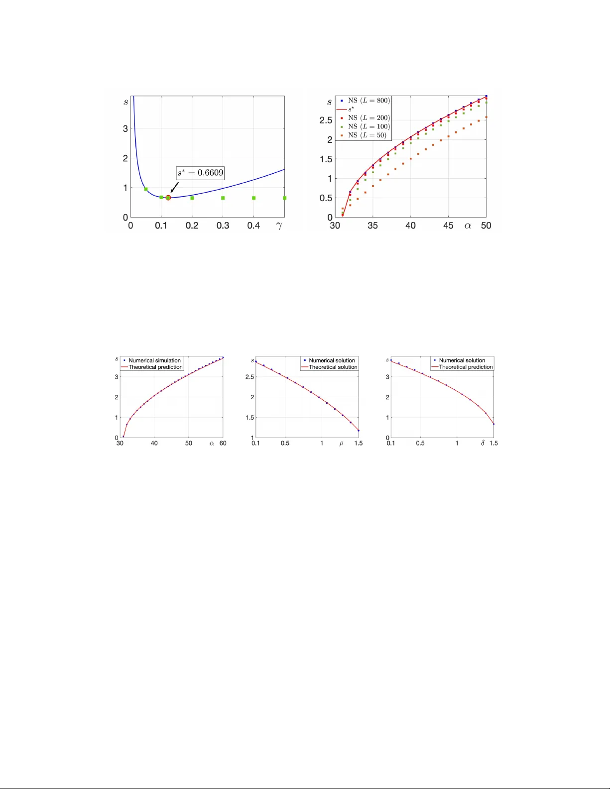
A Damage-Driv en Mo del for Duc henne Muscular Dystroph y: Early-Stage Dynamics and In v asion Thresholds G. Gam bino 1 , F. Gargano 2 , A. Rizzo 1 , V. Sciacca 1 1 Departmen t of Mathematics, Univ ersity of P alermo, Via Archiraﬁ 34, Palermo, 90123, Italy 2 Departmen t of Engineering, Univ ersity of P alermo, Viale delle Scienze, Ed. 8, Palermo, 90128, Italy Abstract W e introduce a spatially extended mathematical mo del for Duc henne muscular dys- troph y based on a damage-driven paradigm, in whic h imm une recruitment is triggered by tissue injury . The mo del is formulated as a reaction–diﬀusion–c hemotaxis system describ- ing the in teraction betw een health y tissue, damaged ﬁbers, imm une cells and inﬂammatory signals. W e establish the global well-posedness of the system and inv estigate the early- stage dynamics through linearization around the healthy equilibrium. Our analysis shows that diﬀusion do es not induce T uring instabilities, so that spatial heterogeneit y cannot arise from diﬀusion-driven mechanisms. Instead, disease progression occurs through in v a- sion pro cesses. W e deriv e explicit conditions for the onset of inv asion, interpreted as an eﬀectiv e damage repro duction threshold and c haracterize the minimal propagation sp eed of pathological fronts, showing that the dynamics is go verned b y a pulled-fron t mec hanism. Numerical simulations supp ort the analytical results and conﬁrm the transition betw een deca y and inv asion. These results provide a mathematical framework for early-stage dis- ease progression and indicate that spatial patterns arise from the expansion of lo calized damage rather than from in trinsic pattern-forming mechanisms. KEYW ORDS : reaction–diﬀusion–chemotaxis system; tra veling fron ts; inv asion thresholds; imm une–tissue in teraction; spatial disease dynamics. 1 In tro duction Duc henne m uscular dystrophy (DMD) is a severe X-linked genetic disorder characterized by progressiv e muscle degeneration and loss of functional tissue [9]. The absence of dystrophin leads to increased mem brane fragilit y , causing recurrent micro-damage of m uscle ﬁbers. These lesions trigger inﬂammatory signaling and immune cell recruitmen t [28, 29, 34], giving rise to a damage–inﬂammation feedbac k lo op that pla ys a cen tral role in disease progression [8]. Exp erimen tal and clinical evidence indicates that imm une activit y in DMD is predomi- nan tly reactive: inﬂammatory resp onses are initiated by tissue damage and tend to subside This is a preprin t v ersion of the man uscript 1 when damage is resolv ed. In the pathological context, how ev er, p ersisten t injury preven ts full reco very , leading to rep eated cycles of degeneration and incomplete repair, with progressive loss of functional tissue [10, 38]. Inﬂammatory signaling can arise ev en before macroscopic degeneration becomes evident. Elev ated lev els of chemokines and inﬂammatory mediators hav e been detected in apparen tly health y m uscle regions of DMD patients [25] and early expression of c hemotactic signals has b een rep orted during the initial stages of muscle injury [15]. These observ ations suggest that early damage and imm une activ ation may precede visible tissue degeneration, motiv ating the study of early-stage dynamical mechanisms. Mathematical modeling has b een used to inv estigate immune–tissue interactions in m uscu- lar dystrophies. More generally , spatially structured mo dels hav e b een increasingly emplo yed to study the interpla y b et ween gro wth, spatial heterogeneit y and biological in teractions in complex systems (see, e.g. [1, 23]). Early approac hes, including predator–prey-type systems, describ e imm une cells as proliferating through direct in teraction with health y tissue [4]. While suc h models capture certain qualitativ e features, they rely on assumptions that are not fully consisten t with experimental observ ations in DMD. In particular, immune recruitment is pri- marily triggered by tissue damage and the asso ciated release of inﬂammatory signals, rather than by direct interaction with intact muscle ﬁb ers. Moreov er, inﬂammatory activity tends to decline when damage is resolved, indicating that imm une dynamics are not self-sustained in the absence of injury . These features are diﬃcult to reconcile with classical predator–prey form ulations, where immune populations grow through direct consumption of health y tissue and may p ersist ev en in the absence of tissue injury . A step to ward greater biological realism was provided by Jarrah et al. [19], who devel- op ed a compartmen tal ODE mo del of immune–m uscle interactions in the mdx mouse, ex- plicitly incorp orating necrotic ﬁb ers, macrophage subp opulations and regeneration. In this framew ork, imm une recruitment is triggered by tissue damage rather than direct in teraction with healthy ﬁbers. Subsequen t mo dels, such as the FRiND mo del [18], further reﬁned this damage-mediated p ersp ectiv e by including detailed recruitment mec hanisms and macrophage plasticit y . Despite these adv ances, most existing mo dels are form ulated as systems of ordinary diﬀer- en tial equations and fo cus primarily on temp oral dynamics [17]. As a consequence, they do not address ho w pathological pro cesses propagate across muscle tissue. Spatial asp ects of disease progression, including the emergence and spread of damaged regions, remain largely unex- plored from a mathematical p ersp ectiv e, despite imaging evidence revealing heterogeneous patterns of degeneration and progressiv e inv asion of aﬀected regions observed in magnetic resonance studies [30, 33]. Spatial propagation phenomena in reaction–diﬀusion systems hav e b een extensiv ely stud- ied since the classical w orks of Fisher and Kolmogoro v–Petro vsky–Piskuno v [11, 20] and fur- ther dev elop ed in the con text of biological in v asions and trav eling w a ves [37, 31]. In this w ork, w e dev elop a mathematical framework for DMD that com bines damage-driven imm une dy- namics with spatial eﬀects. Inspired b y existing ODE-based models, w e in tro duce a reaction 2 system incorp orating tissue capacit y constraints, damage-induced regeneration and saturat- ing immune activ ation. These mechanisms reﬂect fundamental biological features of m uscle repair and inﬂammatory regulation [35, 2]. Most existing mathematical mo dels for DMD fo cus on temp oral dynamics and do not explicitly accoun t for spatial propagation of damage. T o address this limitation, we dev elop a spatially extended damage-driv en framew ork that enables the analytical study of inv asion thresholds and propagation sp eeds in the early stage of disease progression. Within this spatial setting, diﬀusion accounts for lo cal spreading pro cesses, while directed imm une cell migration can b e describ ed through c hemotactic mechanisms. Such mechanisms ha ve b een widely mo deled in the context of cell migration and pattern formation, starting from the classical Keller–Segel framework and its extensions [16, 26] and hav e b een incorp orated in related mo dels of immune-mediated diseases [22]. Accordingly , w e incorp orate a chemotactic term describing directed migration of imm une cells tow ard inﬂammatory signals, reﬂecting the well-established role of c hemokine-guided recruitment in damaged m uscle tissue. A t the same time, w e emphasize that the presen t w ork fo cuses on the early stage of disease progression, where damage and inﬂammatory activity remain small. In this regime, chemo- tactic eﬀects enter only at higher order and do not play a leading role in the onset of inv asion. Early spatial propagation is therefore primarily driven by lo cal damage–inﬂammation feed- bac k mechanisms rather than by directed imm une migration. The inclusion of chemotaxis nev ertheless provides a structurally consistent framew ork that can capture more complex spatial b eha viors in regimes with stronger inﬂammation, which will b e inv estigated in future w ork. The resulting mo del is form ulated as a reaction–diﬀusion–c hemotaxis system describing the spatial ev olution of healthy tissue, damaged ﬁb ers, imm une cells and inﬂammatory signals. W e ﬁrst establish basic analytical prop erties of the system, including p ositivit y , b oundedness, and p ositiv e in v ariance of a biologically admissible domain, ensuring the well-posedness and ph ysical consistency of the model. After nondimensionalization, we characterize the steady states of the system and iden- tify a health y equilibrium together with parameter-dep endent pathological equilibria, when they exist: a healthy state, corresp onding to the absence of damage and inﬂammation, and a diseased state, corresp onding to a pathological regime with p ersisten t damage and inﬂamma- tion. While the healthy equilibrium admits an explicit expression, the diseased equilibrium is determined implicitly through a nonlinear algebraic condition, reﬂecting the complexity of the underlying feedbac k mec hanisms. While the healthy equilibrium admits an explicit expression, the diseased equilibrium is determined implicitly through a nonlinear algebraic condition. A partial analytical c haracterization can b e obtained in a parameter regime con- sisten t with the early-stage scenario, while a complete analysis remains challenging due to the nonlinear coupling of the system. The early-stage dynamics of disease progression are inv estigated through linearization around the healthy equilibrium. W e show that diﬀusion do es not induce pattern-forming in- stabilities of T uring t yp e, indicating that spatial heterogeneity cannot arise through diﬀusion- 3 driv en mec hanisms. Instead, disease progression o ccurs through in v asion pro cesses, in which lo calized damage spreads across the tissue. W e deriv e analytical conditions for the onset of in v asion and characterize the minimal propagation sp eed of pathological fronts. These theoretical predictions are further supp orted b y numerical sim ulations of the full nonlinear system. Our results provide a quan titative description of e arly disease spreading and clarify the mec hanisms go verning spatial progres- sion in DMD. In particular, w e identify an in v asion threshold determining whether lo calized damage can gro w from small p erturbations of the healthy state and c haracterize the mini- mal propagation sp eed of the resulting pathological fronts. Although the reaction dynamics ma y exhibit m ultiple equilibria in certain parameter regimes, w e sho w that, in a biologically relev an t regime consistent with early-stage dynamics, the pathological equilibrium can b e c haracterized more precisely . The onset of spatial spreading considered here is gov erned b y a pulled inv asion mec hanism, controlled b y the linearization around the health y equilibrium. Organization of the pap er. The pap er is organized as follo ws. In section 2, we introduce the dimensional and nondimensionalized mo dels and discuss their biological interpretation. Section 3 is dev oted to the analysis of the spatially homogeneous system, where we estab- lish positivity , inv ariant regions and c haracterize the equilibria together with the stability of the healthy state. In section 4, we study the w ell-p osedness of the full reaction–diﬀusion– c hemotaxis system, proving global existence, uniqueness and b oundedness of solutions within a biologically admissible domain. Section 5 fo cuses on the early-stage spatial dynamics. By linearizing the system around the health y equilibrium, we show the absence of diﬀusion-driv en instabilities and demonstrate that spatial progression occurs through inv asion processes. W e deriv e analytical conditions for the inv asion threshold and characterize the minimal propaga- tion sp eed of pathological fron ts. In section 6, we presen t n umerical simulations of the full nonlinear system, v alidating the analytical predictions and illustrating the in v asion dynamics in one-dimensional domains. Finally , section 7 discusses the biological implications of our ﬁndings and outlines p ossible directions for future researc h. 2 The mo del In this section, we present the mo del and discuss its interpretation. W e consider four state v ariables describing the main pro cesses inv olv ed in DMD: healthy tissue H , damaged tissue D , macrophages M and c hemokines C . This minimal set is chosen to capture the damage- driv en and inﬂammation-mediated nature of the disease, fo cusing on the feedback b et ween tissue injury and imm une response while maintaining analytical tractability . The mo del adopts a damage-driven p ersp ectiv e, where imm une activ ation is initiated b y tissue injury rather than b y direct interaction with healthy ﬁbers. This approac h diﬀers from earlier predator–prey-t yp e mo dels, where immune p opulations gro w through direct in- teraction with intact tissue [4], as w ell as from more detailed mo dels that distinguish multiple imm une subp opulations with diﬀeren t functional roles [18, 19]. In con trast, we adopt an eﬀec- 4 tiv e description in whic h regeneration processes and imm une activity are represented through aggregated v ariables, without introducing additional compartments. Biologically , muscle re- pair inv olv es several in termediate stages, including satellite cell activ ation, diﬀerentiation and fusion, whic h t ypically o ccur on timescales faster than the macroscopic progression of degener- ation considered in this work. These pro cesses can therefore be incorp orated into an eﬀectiv e regeneration mechanism without introducing additional state v ariables. Similarly , the immune resp onse is describ ed through a single macrophage p opulation rather than distinct subt yp es. While macrophage polarization pla ys an imp ortan t biological role, the dominan t eﬀect at the tissue scale is the net inﬂammatory activit y associated with recruited imm une cells. Represen ting this activity through a single eﬀective p opulation captures the leading-order dynamics, while a voiding an unnecessary increase in dimensionality that would complicate the analytical in vestigation of the system. W e therefore propose the following system:                          ∂ τ H = D H ∆ H + ( s + r H D )  1 − H + D K  − µ H H − a ( C ) M H , ∂ τ D = D D ∆ D + a ( C ) M H − µ D D − r H D  1 − H + D K  , ∂ τ M = D M ∆ M − ∇ · ( χ ( C ) M ∇ C ) + r M D − µ M M , ∂ τ C = D C ∆ C + r C D − µ C C, (2.1) where: a ( C ) = ¯ a C + C ϵ k c + C , χ ( C ) = ¯ χ C k χ + C (2.2) and all the parameters are positive. A detailed description of the role of eac h parameter is giv en in T able 1. The mo del incorp orates a constrain t on the total functional tissue through the factor: 1 − H + D K , whic h represents comp etition for limited tissue capacit y . This do es not imply conserv ation of total tissue mass. In the pathological context of DMD, necrosis, immune-mediated clearance and replacemen t b y adip ose or ﬁbrotic tissue lead to an irrev ersible loss of functional m uscle. Accordingly , the carrying capacit y parameter represents an eﬀective upp er b ound on the lo cally sustainable tissue densit y rather than a conserved quan tity . The term: ( s + r H D )  1 − H + D K  describ es tissue main tenance and regeneration. The constan t con tribution s represen ts basal turno ver, while the comp onen t prop ortional to D mo dels damage-induced repair activ ation, reﬂecting the biological observ ation that mo derate injury stim ulates regenerativ e mec hanisms. 5 P arameter Description Biological Role D H , D D Tissue diﬀusion coeﬃcients Spatial expansion of muscle ﬁb ers D M , D C Motilit y coeﬃcients Diﬀusion of imm une and signaling cells s Basal growth rate In trinsic main tenance of health y tissue r H Repair rate Con version rate of damaged ﬁb ers bac k to health y ones K Carrying capacity Maxim um densit y of the tissue µ H , µ D Natural turnov er rates Remo v al rates of health y and damaged tissue ¯ a Maxim um damage rate P eak aggressiv eness of macrophages under inﬂammation C ϵ Basal activ ation Residual damage potential at minimal c hemokines levels k c Half-saturation (damage) Chemokines concentration for half-maximal ﬁber attac k. r M Macrophage recruitment Rate of imm une cell inﬁltration triggered by damage. µ M Macrophage decay Ap optosis or clearance of inﬂammatory cells. ¯ χ Chemotactic sensitivity Strength of directed macrophage migration to w ard C . k χ Chemotactic saturation Sensitivit y threshold for the c hemical gradient. r C Chemokines pro duction Secretion rate of signals by damaged tissue. µ C Chemokines degradation Ap optosis of chemokines. T able 1: Description of mo del parameters and their biological interpretation. The same co eﬃcien t r H app ears in the damaged tissue equation, ensuring mass transfer consistency b et ween compartmen ts at the eﬀective mo deling lev el. Imm une-mediated damage is represented by the interaction term a ( C ) M H , where the function a ( C ) describ es the dependence of tissue destruction on the inﬂammatory state. The saturating structure: a ( C ) = ¯ a C + C ϵ k c + C captures t wo key biological features: the presence of a residual inﬂammatory activit y ev en at low chemokine levels ( C ϵ ) and the saturation of immune aggressiv eness at high signaling concen trations due to physiological limits in cellular activ ation. The macrophage equation reﬂects the damage-driven nature of the immune resp onse. Recruitmen t is prop ortional to the amoun t of damaged tissue ( r M D ), consistent with the release of inﬂammatory mediators from injured ﬁb ers, while linear decay represents clearance and apoptosis. The c hemokine equation follo ws a similar structure, with production driven by tissue damage and degradation accoun ting for molecular turnov er. T ogether, these equations enco de the self-amplifying inﬂammatory lo op characteristic of the disease, in which damage promotes inﬂammation and inﬂammation further increases damage. Spatial eﬀects are in tro duced through diﬀusion and c hemotaxis. Diﬀusion terms accoun t for lo cal spreading pro cesses, including migration of imm une cells, dispersion of signaling molecules and eﬀectiv e spatial redistribution of tissue components associated with remo deling and expansion. The diﬀusion coeﬃcients for tissue v ariables are assumed to b e relativ ely small (see Section 6.1 for details), reﬂecting the limited motilit y of muscle ﬁb ers compared to imm une cells and signaling molecules, while maintaining suﬃcient regularity for mathematical 6 w ell-p osedness of the system. Directed migration of macrophages is modeled through the chemotactic ﬂux: −∇ · ( χ ( C ) M ∇ C ) , where the sensitivit y function χ ( C ) has a saturating form. This structure reﬂects receptor- mediated sensing mec hanisms, with increased resp onsiv eness for w eak signals and saturation at high c hemokine concentrations due to receptor o ccupancy limits. T o reduce the num b er of indep enden t parameters and identify the c haracteristic scales of the system (2.1), w e in tro duce the following set of dimensionless v ariables: t = µ H τ , x = r µ H D H ξ , h = H K , d = D K , m = µ M M r m K , c = C k c . The temp oral scale is chosen according to the characteristic turno ver rate of healthy tissue, while the spatial scale is determined b y the corresp onding diﬀusion length. Tissue densities are normalized by the carrying capacit y and the immune and signaling v ariables are scaled with resp ect to their natural pro duction-deca y balances. The resulting system reads as:                          ∂ t h = ∆ h + ( σ + ρd )(1 − h − d ) − h − α c + c ϵ 1 + c mh, ∂ t d = D d ∆ d + α c + c ϵ 1 + c mh − δ d − ρd (1 − h − d ) , ∂ t m = D m ∆ m − χ 0 ∇ ·  c κ + c m ∇ c  + ν ( d − m ) , ∂ t c = D c ∆ c + r d − µc, (2.3) where: D d = D D D H , D m = D M D H , D c = D C D H , δ = µ D µ H , ν = µ M µ H , µ = µ C µ H , σ = s K µ H , ρ = r H µ H , r = r C K k c µ H , α = ¯ a r M K µ H µ M , χ 0 = ¯ χ k c D H , κ = k χ k c . The dimensionless parameters represent ratios b et w een comp eting biological pro cesses and therefore pro vide insights into the relative imp ortance of the underlying mechanisms. In particular, σ describes the strength of basal tissue main tenance relative to the natural turno ver rate, while ρ quan tiﬁes the eﬃciency of damage-induced regeneration. The parameter α measures the eﬀectiveness of immune-mediated damage compared to the characteristic tissue timescale, whereas δ represents the clearance rate of damaged tissue relativ e to the same scale. The parameters ν and µ describ e, resp ectiv ely , the relaxation rates of macrophages and c hemokines. Finally , χ 0 c haracterizes the intensit y of chemotactic migration relative to diﬀusion and κ represen ts the c hemokine concen tration at whic h c hemotactic sensitivit y 7 reac hes half of its maximal v alue. This nondimensional form ulation highlights the key feedback mec hanisms driving the sys- tem while reducing structural complexit y , facilitating b oth analytical inv estigation and nu- merical exploration. 3 Lo cal dynamics of the reaction system In this section, w e fo cus on the reaction terms of (2.3), namely on the corresp onding spatially homogeneous dynamical system:                      ˙ h = ( σ + ρd )(1 − h − d ) − h − α c + c ϵ 1 + c mh, ˙ d = α c + c ϵ 1 + c mh − δ d − ρd (1 − h − d ) , ˙ m = ν ( d − m ) , ˙ c = rd − µc. (3.1) 3.1 P ositiv e in v ariance of the physical domain W e ﬁrst show that the spatially homogeneous system preserves the biologically admissible state space. In particular, healthy and damaged tissue remain nonnegativ e and cannot exceed the total a v ailable tissue fraction, while macrophages and c hemokines remain nonnegativ e. Theorem 1 Consider system (3.1) . Then the set: D = { ( h, d, m, c ) ∈ R 4 : h ≥ 0 , d ≥ 0 , m ≥ 0 , c ≥ 0 , h + d ≤ 1 } (3.2) is p ositively invariant. Pro of. W e v erify that the vector ﬁeld is in ward p oin ting or tangent on each b oundary comp onen t of D . (i) Boundary h = 0 . In this case, ˙ h = ( σ + ρd )(1 − d ) ≥ 0 , since d ∈ [0 , 1] on D . Hence the vector ﬁeld p oints in ward or is tangen t to the b oundary h = 0. (ii) Boundary d = 0 . In this case, ˙ d = α c + c ϵ 1 + c mh ≥ 0 , so the v ector ﬁeld points in ward or is tangen t to the b oundary d = 0. 8 (iii) Boundary m = 0 . In this case, ˙ m = ν d ≥ 0 , hence tra jectories cannot cross the boundary m = 0 to ward negativ e v alues. (iv) Boundary c = 0 . In this case, ˙ c = rd ≥ 0 , so tra jectories cannot cross the boundary c = 0 to ward negativ e v alues. (v) Boundary h + d = 1 . Let T = h + d . Summing the ﬁrst t wo equations in (3.1) yields: ˙ T = ( σ + ρd )(1 − T ) − h − δ d. Therefore, on the b oundary T = 1, ˙ T | T =1 = − h − δ d ≤ 0 . Th us tra jectories cannot cross the b oundary h + d = 1 out ward. Since the v ector ﬁeld points in ward or is tangent on every comp onen t of the b oundary of D , the set D is p ositiv ely inv ariant. Corollary 2 F or any solution with initial c ondition in D , one has: h ( t ) ≥ 0 , d ( t ) ≥ 0 , m ( t ) ≥ 0 , c ( t ) ≥ 0 h ( t ) + d ( t ) ≤ 1 , for all t ≥ 0 . Lemma 3 (T otal tissue density is strictly b elow saturation at equilibrium) L et ( h ∗ , d ∗ , m ∗ , c ∗ ) ∈ D b e an e quilibrium of system (3.1) . Then: h ∗ + d ∗ < 1 . Pro of. Let T = h + d . Summing the ﬁrst tw o equations of (3.1) giv es: ˙ T = ( σ + ρd )(1 − T ) − h − δ d. A t equilibrium, 0 = ( σ + ρd ∗ )(1 − T ∗ ) − h ∗ − δ d ∗ , where T ∗ = h ∗ + d ∗ . Hence: ( σ + ρd ∗ )(1 − T ∗ ) = h ∗ + δ d ∗ . Since δ > 0, the identit y h ∗ + δ d ∗ = 0 implies h ∗ = d ∗ = 0. But this cannot o ccur at equilibrium, since in that case one would also hav e m ∗ = c ∗ = 0 and therefore ˙ h = σ  = 0. Since σ + ρd ∗ > 0, it follows that 1 − T ∗ > 0 , 9 that is, h ∗ + d ∗ < 1 . 3.2 Classiﬁcation of equilibria W e now c haracterize the equilibria of system (3.1) and discuss their stability prop erties. 3.2.1 Health y equilibrium The system alw a ys admits the healthy equilibrium: H ⋆ = ( h 0 , 0 , 0 , 0) , where h 0 = σ 1 + σ . (3.3) The Jacobian matrix at H ⋆ is: J ( H ⋆ ) =        − (1 + σ ) ρ 1 + σ − σ − αc ϵ h 0 0 0 − δ − ρ 1 + σ αc ϵ h 0 0 0 ν − ν 0 0 r 0 − µ        . The eigenv alues asso ciated with the h - and c -comp onen ts are − (1 + σ ) and − µ , and are therefore strictly negativ e. The stability of H ⋆ is thus determined b y the coupled ( d, m ) subsystem. The corresp onding characteristic p olynomial is: λ 2 + a 1 λ + a 0 , with: a 1 = δ + ν + ρ 1 + σ > 0 , a 0 = ν  δ + ρ 1 + σ − αc ϵ σ 1 + σ  . Therefore, the sign of a 0 determines the stabilit y of H ⋆ . In tro ducing the quan tit y: Θ := δ (1 + σ ) + ρ − α c ϵ σ, (3.4) w e obtain: a 0 = ν 1 + σ Θ . The healthy equilibrium H ⋆ is thus lo cally asymptotically stable if Θ > 0 and loses stability at Θ = 0. This threshold coincides with the inv asion condition derived from the linearized reaction– diﬀusion system (see Remark 21). 10 3.2.2 P athological equilibria Besides the healthy equilibrium, solutions with d ∗ > 0 ma y arise. A t equilibrium, the last tw o equations of (3.1) yield: m ∗ = d ∗ , c ∗ = r µ d ∗ . (3.5) Moreo ver, imp osing ˙ h + ˙ d = 0 giv es: ( σ + ρd ∗ )(1 − h ∗ − d ∗ ) − h ∗ − δ d ∗ = 0 , from which w e obtain: h ∗ = σ − ( σ + δ ) d ∗ 1 + σ . (3.6) Therefore, any pathological equilibrium m ust b e of the form: D ⋆ =  σ − ( σ + δ ) d ∗ 1 + σ , d ∗ , d ∗ , r µ d ∗  , (3.7) where d ∗ is determined b y substituting (3.6) into the condition ˙ d = 0. This leads to the quadratic equation: G ( d ∗ ) = 0 , with G ( d ) := g 2 d 2 + g 1 d + g 0 , (3.8) and g 2 = r  ρ (1 − δ ) − α ( δ + σ )  , (3.9) g 1 = − δ ( r + µρ + r σ ) + µρ − r ( ρ − ασ ) − αµ ( δ + σ ) c ϵ , (3.10) g 0 = − µ ( δ + ρ + δ σ ) + αµc ϵ σ. (3.11) The num b er of pathological equilibria is determined by the ro ots of (3.8) for whic h the corresp onding equilibrium D ⋆ lies in the inv ariant set D deﬁned in (3.2). Dep ending on the parameter v alues, up to tw o suc h equilibria may o ccur. Although a complete analytical classiﬁcation of (3.8) is diﬃcult in general, a sharp er result can b e obtained in the regime δ ≥ 1, whic h is consisten t with the early-stage scenario considered in this work. Prop osition 4 Assume δ ≥ 1 and Θ < 0 , with Θ given in (3.4) . Then e quation (3.8) admits a unique p ositive r o ot d ∗ and this r o ot satisﬁes: 0 < d ∗ < σ σ + δ . (3.12) In p articular, the c orr esp onding e quilibrium D ⋆ , as deﬁne d in (3.7) , b elongs to the invariant set D in (3.2) . Pro of. F rom the deﬁnition of Θ in (3.4), the condition Θ < 0 implies g 0 > 0, where g 0 is giv en in (3.11). 11 Moreo ver, since δ ≥ 1, we ha ve g 2 < 0, see (3.9). Hence g 2 g 0 < 0 and therefore the quadratic p olynomial G ( d ) admits tw o distinct real roots of opposite sign. In particular, there exists a unique p ositiv e root d ∗ . Let: ˜ d := σ σ + δ . A direct computation shows that G ( ˜ d ) < 0, while G (0) = g 0 > 0. By con tinuit y , the p ositiv e ro ot d ∗ lies in (0 , ˜ d ) and hence satisﬁes (3.12). Using (3.6), this implies h ∗ > 0. Moreov er, since δ ≥ 1 and d ∗ > 0, w e ha ve: h ∗ + d ∗ = σ + (1 − δ ) d ∗ 1 + σ < 1 . Finally , from (3.5) w e obtain m ∗ > 0 and c ∗ > 0. Hence D ⋆ ∈ D . The ov erall structure of pathological equilibria in the parameter plane ( δ, α ) is illustrated in Fig. 1. While multiple equilibria may arise in the general case, the previous result shows that, for δ ≥ 1, a unique biologically admissible equilibrium exists ab o ve the inv asion threshold. Figure 1: Numerically computed bifurcation diagram in the ( δ, α ) parameter plane. The solid blac k line corresp onds to the threshold condition Θ = 0, with Θ given in (3.4), separating regions with diﬀeren t stabilit y prop erties of the health y equilibrium. In the white region, the health y equilibrium is stable and no biologically admissible pathological equilibrium exists. In the blue region, the healthy equilibrium is unstable and a stable pathological equilibrium exists. The green region corresp onds to a bistable regime, where the health y equilibrium co exists with tw o pathological equilibria, one stable and one unstable. In the yello w region (b elo w the threshold line), the health y equilibrium is stable and co exists with t wo pathological equilibria, b oth unstable. In the magenta region (abov e the threshold line), b oth the health y equilibrium and the pathological equilibrium are unstable. The parameters are c hosen as σ = 1, ρ = 0 . 9, c ϵ = 0 . 1, ν = 7, k = r = 1, µ = 168, D d = 1, D m = 10, D c = 1000 and χ 0 = 5. More precisely , the black line corresp onds to the threshold condition Θ = 0, with Θ given in (3.4), whic h determines the loss of stabilit y of the healthy equilibrium. In the white region, the health y equilibrium is stable and no biologically admissible patho- logical equilibrium exists. In the blue region, the health y equilibrium is unstable and a stable pathological equilibrium emerges, corresp onding to a regime of p ersisten t damage. 12 F or suﬃcien tly small v alues of δ , a bistable regime app ears (green region), in which the health y equilibrium co exists with t wo pathological equilibria, one stable and one unstable. This indicates the possibility of threshold-driven transitions b et ween recov ery and sustained degeneration. In the y ello w region (b elo w the threshold line), the health y equilibrium remains stable and co exists with tw o pathological equilibria, b oth unstable. In the magen ta region (ab o ve the threshold line), the health y equilibrium is unstable and a single pathological equilibrium exists, whic h is also unstable. This regime is particularly notew orthy: although no stable equilibrium is a v ailable, numerical sim ulations (not sho wn here) indicate that the long-term b eha vior depends on the amplitude of the initial p erturba- tion. In particular, suﬃcien tly small p erturbations may deca y tow ard the healthy state, while larger perturbations can trigger spatial in v asion and the formation of propagating fron ts. This suggests that, in this parameter range, the long-term dynamics dep ends on the amplitude of the initial p erturbation. While small perturbations may relax to w ard the healthy state, larger p erturbations can trigger spatial in v asion and the formation of propagating fron ts, consisten tly with the pulled-fron t b eha vior iden tiﬁed in Section 5. W e emphasize that the regimes highligh ted in the zo omed region of Fig. 1 corresp ond to small v alues of δ , asso ciated with slow damage clearance and are therefore not representativ e of the early-stage dynamics considered in this work. A complete analytical description of (3.8) remains challenging in general, due to the additional constrain ts 0 < h ∗ + d ∗ ≤ 1 and the nonlinear dep endence on the parameters. In particular, a full characterization of the b elow-threshold regime appears to require additional conditions on the co eﬃcien ts of (3.8). F or this reason, in the following we fo cus on the dynamics near the healthy equilibrium and on the early-stage regime, where the onset of disease progression can b e analyzed through linear mechanisms. 4 W ell-p osedness of the reaction–diﬀusion–c hemotaxis system In this section, we establish the global well-posedness of the reaction–diﬀusion–chemotaxis system (2.3). In particular, w e pro ve the existence, uniqueness and b oundedness of solutions, together with the preserv ation of a biologically admissible domain, ensuring that all compo- nen ts remain non-negative and that the saturation constraint h + d ≤ 1 is satisﬁed for all times. These results hold indep enden tly of the sp eciﬁc dynamical regime and pro vide the analytical framework required for the subsequen t in v estigation of the system dynamics. The analysis relies on a Lera y–Sc hauder ﬁxed point argument, com bined with a priori esti- mates and parabolic regularit y techniques. These results pro vide the mathematical framew ork required for the subsequen t in v estigation of the dynamical prop erties of the mo del. F or the well-posedness analysis, w e rewrite the dimensionless system in the following form: 13          ∂ t h = ∆ h + ( σ + ρd )(1 − h − d ) − h − A ( m, c ) h , ( t, x ) ∈ Ω T ∂ t d = D d ∆ d + A ( m, c ) h − δ d − ρd (1 − h − d ) , ( t, x ) ∈ Ω T ∂ t m = D m ∆ m − ∇ · ( χ ( m, c ) ∇ c ) + ν ( d − m ) , ( t, x ) ∈ Ω T ∂ t c = D c ∆ c + r d − µc, ( t, x ) ∈ Ω T , (4.1) with χ ( m, c ) = χ 0 m c κ + c , A ( m, c ) = α c + c ϵ 1 + c m , (4.2) and w e denote b y Ω T = (0 , T ) × Ω, where Ω is a b ounded domain in R n ( n ∈ N , n ≥ 1) with smo oth, sp eciﬁed later, b oundary ∂ Ω. W e denote by n = n ( s ) the out ward normal to ∂ Ω at a p oin t s of the boundary , and imp ose the following Neumann b oundary condition on ∂ Ω:              n ( s ) · ∇ h ( t, s ) = 0 , ( t, s ) ∈ (0 , T ) × ∂ Ω , n ( s ) · ∇ d ( t, s ) = 0 , ( t, s ) ∈ (0 , T ) × ∂ Ω , n ( s ) · ∇ m ( t, s ) = 0 , ( t, s ) ∈ (0 , T ) × ∂ Ω , n ( s ) · ∇ c ( t, s ) = 0 , ( t, s ) ∈ (0 , T ) × ∂ Ω . (4.3) Finally , we imp ose the following non-negativ e initial conditions:              h ( t = 0 , x ) = h in ( x ) , x ∈ Ω , d ( t = 0 , x ) = d in ( x ) , x ∈ Ω , m ( t = 0 , x ) = m in ( x ) , x ∈ Ω , c ( t = 0 , x ) = c in ( x ) , x ∈ Ω , (4.4) and we supp ose that the follo wing condition holds h in ( x ) + d in ( x ) ≤ 1 , x ∈ Ω . (4.5) Moreo ver, w e recall that all system parameters are positive. W e introduce the functional framework used throughout the section (see [14, 21]). F or 1 ≤ p ≤ ∞ , w e denote b y L p (Ω) the usual Lebesgue spaces with norm ∥ · ∥ L p (Ω) and b y L p (Ω T ) = L p ((0 , T ); L p (Ω)) the corresp onding space-time spaces, equipp ed with the norm ∥ · ∥ L p (Ω T ) . More generally , for 0 ≤ t 0 < T , we set Ω t 0 ,T = ( t 0 , T ) × Ω and deﬁne L p (Ω t 0 ,T ) accordingly . W e denote b y W r,p (Ω) the Sob olev spaces of order r with in tegrability p . F or the parabolic setting, we consider the space W 1 , 2 p (Ω t 0 ,T ) = { v : ∂ r t ∂ s x v ∈ L p (Ω t 0 ,T ) , 2 r + s ≤ 2 } , endo wed with the norm ∥ v ∥ W 1 , 2 p (Ω t 0 ,T ) = X 2 r + s ≤ 2 ∥ ∂ r t ∂ s x v ∥ L p (Ω t 0 ,T ) . 14 W e also denote by C k (Ω) the space of functions with contin uous deriv ativ es up to order k , and by C 0 (Ω T ) the space of contin uous functions in Ω T . Finally , we in tro duce the space C 0 , 1 = C 0 , 1 ([0 , T ] × Ω) of functions that are contin uous together with their spatial gradients, endo wed with the norm ∥ u ∥ C 0 , 1 = sup t ∈ [0 ,T ] ∥ u ( t, · ) ∥ L ∞ (Ω) + sup t ∈ [0 ,T ] ∥∇ u ( t, · ) ∥ L ∞ (Ω) . F or a Banac h space X , we denote by [ X ] m the Cartesian pro duct of m copies of X , endo wed with the natural norm. Our main w ell-p osedness result is stated in the follo wing theorem. Theorem 5 L et Ω b e a smo oth ( C 2+ η , for some η > 0 ) b ounde d c onne cte d op en subset of R n , with n ∈ N and n ≥ 1 . F or ˜ p > n + 2 , let the non-ne gative initial c onditions ( h in , d in , m in , c in ) ∈ [ W (2 − 2 / ˜ p ) , ˜ p (Ω)] 4 , with (4.5) , then the system (4.1) admits a unique glob al str ong solution which is non-ne gative in e ach c omp onent, with h + d ≤ 1 in Ω and b ounde d in time. Mor e pr e cisely, we have t hat: ∂ t ( h, d, m, c ) , ∆( h, d, m, c ) ∈ [ L ˜ p (Ω T )] 4 , ∇ · ( χ ( m, c ) ∇ c ) ∈ L ˜ p (Ω T ) , and ( h, d, m, c ) ∈ [ C 0 , 1 ] 4 , for al l T > 0 . F urthermor e, if ( h in , d in , m in , c in ) ∈ [ C 2 ( Ω)] 4 , non ne gative with (4.5) , and ∇ h in · n = ∇ d in · n = ∇ m in · n = ∇ c in · n = 0 on ∂ Ω , then the solution to the system (4.1) is classic al, i.e., ∀ T > 0 , ∂ t ( h, d, m, c ) , ∆( h, d, m, c ) ∈ [ C 0 (Ω T )] 4 , ∇ · ( χ ( m, c ) ∇ c ) ∈ C 0 (Ω T ) . Mor e over, ther e exists a c onstant C > 0 , dep ending on Ω , h in , d in , m in , c in and on al l the system p ar ameters, such that, the unique glob al solution of the system (4.1) satisﬁes: sup t ≥ 0 ∥ ( h ( t, · ) , d ( t, · ) , m ( t, · ) , c ( t, · )) ∥ [ W 1 , ∞ (Ω)] 4 ≤ C , (4.6) and lim sup t → + ∞ ∥ ( h ( t, · ) , d ( t, · ) , m ( t, · ) , c ( t, · )) ∥ [ W 1 , ∞ (Ω)] 4 ≤ C . (4.7) The pro of of Theorem 5 is divided into three parts. In Subsection 4.1 w e prov e the global existence of solutions b y means of a Lera y–Schauder ﬁxed p oin t argument. In Subsection 4.2 w e establish uniqueness, while in Subsection 4.3 we derive the uniform-in-time b ounds (4.6)– (4.7). The argumen t follows the approac h developed in [5, 12], adapted here to the sp eciﬁc structure of the reaction-diﬀusion system (4.1). W e recall the follo wing embedding lemma, whic h will b e used in the sequel (see [21, 32]). 15 Lemma 6 L et 1 < p < ∞ , 0 ≤ t 0 < T , and Ω b e a b ounde d domain in R n . Then ther e exists a c onstant C T > 0 , dep ending on T − t 0 , Ω , p , and n , such that for al l u ∈ W 1 , 2 p (Ω t 0 ,T ) the fol lowing estimates hold: • ∥ u ∥ L q (Ω t 0 ,T ) ≤ C T ∥ u ∥ W 1 , 2 p (Ω t 0 ,T ) , wher e        q = ( n +2) p n +2 − 2 p if p < n +2 2 q = ∞ if p > n +2 2 q is ﬁnite and arbitr ary if p = n +2 2 (4.8) • ∥∇ u ∥ L q (Ω t 0 ,T ) ≤ C T ∥ u ∥ W 1 , 2 p (Ω t 0 ,T ) , wher e        q = ( n +2) p n +2 − p if p < n + 2 q = ∞ if p > n + 2 q is ﬁnite and arbitr ary if p = n + 2 (4.9) • W 1 , 2 p (Ω t 0 ,T ) is c omp actly emb e dde d in C 0 , 1 , if p > n + 2 . 4.1 Global existence of solutions In this section, we prov e the global existence of non-negativ e solutions to system (4.1) by means of a Leray–Sc hauder ﬁxed p oint argumen t. W e also deriv e uniform b ounds in the L ∞ norm. The pro of is structured as follo ws. W e ﬁrst construct a suitable map S and establish its compactness and contin uit y . W e then in tro duce the set Φ of its ﬁxed p oin ts and pro ve that its elemen ts are non-negative and satisfy the saturation constraint. Finally , we show that Φ is b ounded and conclude the existence result. 4.1.1 Construction of the map S W e b egin b y constructing a suitable solution operator S , whic h will be used to apply the Lera y–Schauder ﬁxed p oin t theorem. S : [ C 0 , 1 ] 4 × [0 , 1] − → [ C 0 , 1 ] 4 , (4.10) as follows. Giv en ( h, d, m, c ) ∈ [ C 0 , 1 ] 4 and λ ∈ [0 , 1], w e deﬁne S ( h, d, m, c, λ ) = ( λ h ∗ , λ d ∗ , λ m ∗ , λ c ∗ ) , (4.11) 16 where ( h ∗ , d ∗ , m ∗ , c ∗ ) is obtained b y solving, in sequence, the follo wing linear parab olic prob- lems. F or a giv en d ∈ C 0 , 1 , we consider the problem        ∂ t c ∗ = D c ∆ c ∗ − µc ∗ + r d + ( t, x ) ∈ Ω T , n · ∇ c ∗ = 0 ( t, s ) ∈ (0 , T ) × ∂ Ω , c ∗ ( t = 0 , x ) = c in ( x ) x ∈ Ω , (4.12) where d + = max(0 , d ). Once c ∗ is determined, for giv en m, c ∈ C 0 , 1 w e solv e        ∂ t m ∗ = D m ∆ m ∗ − ∇ · ( χ ( m + , c + ) ∇ c ∗ ) + ν ( d + − m ∗ ) ( t, x ) ∈ Ω T , n · ∇ m ∗ = 0 ( t, s ) ∈ (0 , T ) × ∂ Ω , m ∗ ( x, 0) = m in ( x ) x ∈ Ω , (4.13) where m + = max(0 , m ) and c + = max(0 , c ). Next, for giv en h, d ∈ C 0 , 1 , we solv e        ∂ t d ∗ = D d ∆ d ∗ − δ d ∗ − ρd ∗ + ρd + ( h + d ) + + A ( m ∗ , c + ) h + ( t, x ) ∈ Ω T , n · ∇ d ∗ = 0 ( t, s ) ∈ (0 , T ) × ∂ Ω , d ∗ ( x, 0) = d in ( x ) x ∈ Ω , (4.14) where h + = max(0 , h ) and ( h + d ) + = max(0 , h + d ) ∧ min(1 , h + d ). Finally , we consider        ∂ t h ∗ = ∆ h ∗ − h ∗ − A ( m + , c + ) h ∗ + σ (1 − ( h + d ) + ) + ρd ∗ (1 − ( h + d ) + ) ( t, x ) ∈ Ω T , n · ∇ h ∗ = 0 ( t, s ) ∈ (0 , T ) × ∂ Ω , h ∗ ( x, 0) = h in ( x ) x ∈ Ω . (4.15) By construction, the map S associates to each ( h, d, m, c, λ ) an elemen t of [ C 0 , 1 ] 4 . Moreo ver, from the deﬁnition of S given b y (4.12)–(4.15) and the maximal regularit y theory for parabolic equations with Neumann boundary conditions (see [5, 21]), we obtain ∥ ( h ∗ , d ∗ , m ∗ , c ∗ ) ∥ [ W 1 , 2 p (Ω T )] 4 ≤ K ∗ , (4.16) where K ∗ dep ends on T , Ω, n , p , the initial data, the parameters of the system, and the C 0 , 1 norms of h , d , m and c . Since p > n + 2, the space W 1 , 2 p (Ω T ) is compactly em b edded in C 0 , 1 (Lemma 6), and therefore ( h ∗ , d ∗ , m ∗ , c ∗ ) ∈ [ C 0 , 1 ] 4 . 17 4.1.2 Compactness and con tinuit y of S T o apply the Lera y–Schauder ﬁxed p oin t theorem, we prov e that the map S is compact and con tinuous in [ C 0 , 1 ] 4 . W e proceed in t w o steps. In Lemma 7, w e sho w that S maps b ounded sets of [ C 0 , 1 ] 4 × [0 , 1] in to precompact sets of [ C 0 , 1 ] 4 . In Lemma 8, w e pro v e that S is con tinuous. Lemma 7 Under the hyp otheses of The or em 5, the map S maps b ounde d sets of [ C 0 , 1 ] 4 × [0 , 1] into pr e c omp act sets of [ C 0 , 1 ] 4 . Pro of. The claim follo ws from (4.16). Since p > n + 2, the space W 1 , 2 p (Ω T ) is compactly em b edded in C 0 , 1 b y Lemma 6, which yields the desired precompactness. Lemma 8 Under the hyp otheses of The or em 5, the map S is c ontinuous. Pro of. Let ( h 1 , d 1 , m 1 , c 1 ) , ( h 2 , d 2 , m 2 , c 2 ) ∈ [ C 0 , 1 ] 4 . W e start by estimating the diﬀerence c ∗ 1 − c ∗ 2 . F rom (4.12), using maximal regularit y (see [21]) together with the embedding properties of W 1 , 2 p (Lemma 6) for p > n + 2, w e obtain ∥ c ∗ 1 − c ∗ 2 ∥ C 0 , 1 ≤ C ∗ T ∥ d 1+ − d 2+ ∥ L p (Ω T ) ≤ C ∗ T ∥ d 1 − d 2 ∥ C 0 , 1 , (4.17) where C ∗ T denotes a constant dep ending on T , Ω, n , the initial data and the parameters of the system. W e now turn to the estimate of m ∗ 1 − m ∗ 2 , using (4.13). The following p oin twise estimate holds: |∇ · ( χ ( m 1+ , c 1+ ) ∇ c ∗ 1 − χ ( m 2+ , c 2+ ) ∇ c ∗ 2 ) | ≤ ≤ χ 0 | m 1+ | | ∆( c ∗ 1 − c ∗ 2 ) | + χ 0 |∇ m 1+ | |∇ c ∗ 1 − ∇ c ∗ 2 | + + χ 0 | m 1+ − m 2+ | | ∆ c ∗ 2 | + χ 0 |∇ ( m 1+ − m 2+ ) | |∇ c ∗ 2 | . Applying the same argumen ts used for c ∗ 1 − c ∗ 2 , we deduce ∥ m ∗ 1 − m ∗ 2 ∥ C 0 , 1 ≤ C T ( ∥ d 1 − d 2 ∥ C 0 , 1 + ∥ m 1 − m 2 ∥ C 0 , 1 ) , (4.18) where C ∗ T dep ends on T , Ω, n , the initial data and the parameters of the system. W e ﬁnally estimate d ∗ 1 − d ∗ 2 and h ∗ 1 − h ∗ 2 using (4.14) and (4.15). W e ﬁrst establish the follo wing auxiliary estimates: | A ( m ∗ 1 , c 1+ ) h 1+ − A ( m ∗ 2 , c 2+ ) h 2+ | ≤ α (1 + c ϵ ) ( h 2+ | m ∗ 1 − m ∗ 2 | + | m ∗ 1 || h 1+ − h 2+ | ) + + α h 2+ | m ∗ 1 | | 1 − c ϵ || c 1+ − c 2+ | , (4.19)    ρd 1+ ( h 1 + d 1 ) + − ρd 2+ ( h 2 + d 2 ) +    ≤ ≤ ρd 2+ ( | h 1+ − h 1+ | + | d 1+ − d 2+ | ) + ρ ( h 1+ + d 1+ ) | d 1+ − d 2+ | , (4.20) 18 | A ( m 1+ , c 1+ ) h ∗ 1 − A ( m 2+ , c 2+ ) h ∗ 2 | ≤ α (1 + c ϵ ) ( h ∗ 2 | m 1+ − m 2+ | + m 1+ | h 1+ − h 2+ | ) + + α m 1+ | h ∗ 2 | | 1 − c ϵ || c 1+ − c 2+ | , (4.21) | ( h 1 + d 1 ) + ) − ( h 2 + d 2 ) + | ≤ ( | h 1+ − h 2+ | + | d 1+ − d 2+ | ) , (4.22)    ρd ∗ 1 (1 − ( h 1 + d 1 ) + ) − ρd ∗ 2 (1 − ( h 2 + d 2 ) + )    ≤ ≤ ρd ∗ 2 ( | h 1+ − h 2+ | + | d 1+ − d 2+ | ) + ρ (1 + h 1+ + d 1+ )) | d ∗ 1 − d ∗ 2 | . (4.23) Using (4.19)–(4.23) together with the same arguments as b efore, we obtain ∥ d ∗ 1 − d ∗ 2 ∥ C 0 , 1 ≤ C T ( ∥ h 1 − h 2 ∥ C 0 , 1 + ∥ d 1 − d 2 ∥ C 0 , 1 + ∥ m 1 − m 2 ∥ C 0 , 1 + ∥ c 1 − c 2 ∥ C 0 , 1 ) , (4.24) and ∥ h ∗ 1 − h ∗ 2 ∥ C 0 , 1 ≤ C T ( ∥ h 1 − h 2 ∥ C 0 , 1 + ∥ d 1 − d 2 ∥ C 0 , 1 + ∥ m 1 − m 2 ∥ C 0 , 1 + ∥ c 1 − c 2 ∥ C 0 , 1 ) , (4.25) where C ∗ T dep ends on T , Ω, n , the initial data and the parameters of the system. Com bining (4.17), (4.18), (4.24) and (4.25), we conclude that the map S is con tinuous. 4.1.3 The set Φ T o apply the Lera y–Schauder theorem, we in tro duce the set Φ: Φ =  ( h, d, m, c ) ∈ [ C 0 , 1 ] 4 : S ( h, d, m, c, λ ) = ( h, d, m, c ) , 0 < λ ≤ 1  . (4.26) By deﬁnition, if ( h, d, m, c ) ∈ Φ, then h = λh ∗ , d = λd ∗ , m = λm ∗ and c = λc ∗ , where h ∗ , d ∗ , m ∗ and c ∗ solv e (4.15), (4.14), (4.13) and (4.12), resp ectiv ely . Using again the deﬁnition of Φ, and m ultiplying equations (4.15), (4.14), (4.13) and (4.12) b y λ , w e deduce that, if ( h, d, m, c ) ∈ Φ, then ( h, d, m, c ) satisﬁes the following system:              ∂ t h = ∆ h − h − A ( m + , c + ) h + λσ (1 − ( h + d ) + ) + ρd (1 − ( h + d ) + ) , ( t, x ) ∈ Ω T , ∂ t d = D d ∆ d − ( δ + ρ ) d + A ( m, c + ) h + ρλd + ( h + d ) + , ( t, x ) ∈ Ω T , ∂ t m = D m ∆ m − ∇ · ( χ ( m + , c + ) ∇ c ) + ν ( λd + − m ) , ( t, x ) ∈ Ω T , ∂ t c = D c ∆ c − µc + r λd + , ( t, x ) ∈ Ω T , (4.27) with b oundary conditions n · ∇ h ( t, s ) = n · ∇ d ( t, s ) = n · ∇ m ( t, s ) = n · ∇ c ( t, s ) = 0 ( t, s ) ∈ (0 , T ) × ∂ Ω (4.28) 19 and initial conditions              h (0 , x ) = λh in ( x ) x ∈ Ω , d (0 , x ) = λd in ( x ) x ∈ Ω , m (0 , x ) = λm in ( x ) x ∈ Ω , c (0 , x ) = λc in ( x ) x ∈ Ω , (4.29) whic h are non-negative and satisfy the saturation condition (4.5). W e ﬁrst establish the follo wing Lemma. Lemma 9 If ( h, d, m, c ) ar e in Φ , then they ar e non-ne gative. Pro of. Since c in ≥ 0 and d + ≥ 0, then c ≥ 0. T o pro ve that m ≥ 0, we m ultiply the equation for m by m 2 − , with m − = max(0 , − m ) and integrate in space and time. Recalling that m in ≥ 0, w e obtain: − 1 3 Z Ω m 3 − dx = 2 D m Z t 0 Z Ω m − |∇ m − | 2 dxdt − ν Z t 0 Z Ω mm 2 − dxdt + ν λ Z t 0 Z Ω d + m 2 − dxdt − 2 χ 0 Z t 0 Z Ω cm − m + 1 + c ∇ m − · ∇ cdxdt ≥ 2 Z t 0 Z Ω m − |∇ m − | 2 dxdt + ν Z t 0 Z Ω m 3 − dxdt ≥ 0 , and consequently m − = 0 for eac h t ∈ [0 , T ]. W e pro ceed analogously for h and d , obtaining: − 1 3 Z Ω d 3 − dx = 2 D d Z t 0 Z Ω d − |∇ d − | 2 dxdt + ( δ + ρ ) Z t 0 Z Ω d − d 2 − + + λρ Z t 0 Z Ω d + ( h + d ) + d 2 − dxdt + Z t 0 Z Ω A ( m, c + ) h + d 2 − dxdt ≥ 0 , − 1 3 Z Ω h 3 − dx = 2 Z t 0 Z Ω h − |∇ h − | 2 dxdt + λσ Z t 0 Z Ω (1 − ( h + d ) + ) h 2 − dxdt + Z t 0 Z Ω h 3 − dxdt + Z t 0 Z Ω A ( m + , c + ) h 3 − dxdt + ρ Z t 0 Z Ω d (1 − ( h + d ) + ) h 2 − dxdt ≥ 0 , using that h in ≥ 0 and d in ≥ 0. Hence h − = 0 and d − = 0 for eac h t ∈ [0 , T ]. By Lemma 9, system (4.27) reduces to:              ∂ t h = ∆ h − h − A ( m, c ) h + λσ (1 − ( h + d ) + ) + ρd (1 − ( h + d ) + ) , ( t, x ) ∈ Ω T , ∂ t d = D d ∆ d − ( δ + ρ ) d + A ( m, c ) h + ρλd ( h + d ) + , ( t, x ) ∈ Ω T , ∂ t m = D m ∆ m − ∇ · ( χ ( m, c ) ∇ c ) + ν ( λd − m ) , ( t, x ) ∈ Ω T , ∂ t c = D c ∆ c − µc + r λd , ( t, x ) ∈ Ω T , (4.30) 20 with b oundary conditions (4.28) and non-negative initial data (4.29) with condition (4.5). 4.1.4 Boundedness of Φ W e now show that Φ is b ounded in [ C 0 , 1 ] 4 (see Lemma 13 b elow). T o this end, w e ﬁrst establish t wo auxiliary lemmas describing the regularit y of h , d , m , and c for ( h, d, m, c ) ∈ Φ. W e then derive a sequence of a priori estimates, which will b e used to prov e the b ound- edness of the set of ﬁxed p oin ts and to conclude the existence argument. Lemma 10 L et ( h, d, m, c ) ∈ Φ . Under the hyp otheses of The or em 5, ther e exists a c onstant H 1 , dep ending on T , Ω , n , the initial data and the p ar ameters of the system, but not on λ , such that sup t ∈ [0 ,T ] ∥ ( h ( t, · ) , d ( t, · ) , m ( t, · ) , c ( t, · )) ∥ L 1 (Ω) ≤ H 1 . (4.31) Pro of. In tegrating the equations for h and d in (4.30) and summing, we obtain ∂ t Z Ω ( h + d ) dx ≤ σ Z Ω (1 − ( h + d ) + ) dx ≤ σ | Ω | . (4.32) Here | Ω | denotes the measure of the domain. Applying Gron wall’s lemma and using that h in + d in ≤ 1, w e conclude that h and d are bounded in L 1 (Ω). In tegrating the equations for m and c in (4.30), w e obtain d dt Z Ω m dx ≤ − ν Z Ω m dx + ν ∥ d ∥ L 1 (Ω) , (4.33) and d dt Z Ω c dx ≤ − µ Z Ω c dx + r ∥ d ∥ L 1 (Ω) . (4.34) Applying Gronw all’s lemma, w e obtain (4.31). W e now deriv e a regularit y estimate for c , whic h will be used in the sequel. Lemma 11 L et ( h, d, m, c ) ∈ Φ . Under the hyp otheses of The or em 5, ther e exists a c onstant H ∗ , dep ending on Ω , T , n , the initial data and the p ar ameters of the system, but not on λ , such that ∥ c ∥ W 2 , 1 1 (Ω T ) ≤ H ∗ , (4.35) and ∥∇ c ∥ L ( n +2) / ( n +1) (Ω T ) ≤ H ∗ . (4.36) Pro of. Estimate (4.35) follows from the equation for c in (4.30), using maximal regularit y for the heat equation together with (4.31). Estimate (4.36) then follows from (4.35) b y the em b edding Lemma 6 (see [5]). 21 W e no w extend the previous estimates to L p b ounds for the solution components by means of a dualit y argument. Lemma 12 L et ( h, d, m, c ) ∈ Φ . Under the hyp otheses of The or em 5, for any 1 ≤ p < ∞ , ther e exists a c onstant H p , dep ending on p , Ω , T , n , the initial data and the p ar ameters of the system, but not on λ , such that ∥ h ∥ L p (Ω T ) + ∥ d ∥ L p (Ω T ) + ∥ m ∥ L p (Ω T ) ≤ H p . (4.37) Pro of. The pro of follo ws [5, 12] (see also [3, 6, 7, 24, 27]). W e pro ve (4.37) for p large enough, namely for p = p ′ / ( p ′ − 1), where p ′ satisﬁes 1 < p ′ < n +2 2 . Consequen tly , w e hav e 1 + 2 n < p < ∞ . W e pro ceed b y a dualit y argument. Let θ ∈ L p ′ (Ω T ) b e suc h that θ ≥ 0 and ∥ θ ∥ L p ′ (Ω T ) ≤ 1. W e denote b y ψ D the unique solution of the follo wing backw ard heat equation:        ∂ ∂ t ψ D + D ∆ ψ D = − θ ( t, x ) ∈ Ω T , ∇ ψ D · n = 0 ( t, s ) ∈ (0 , T ) × ∂ Ω , ψ D ( T , x ) = 0 x ∈ Ω , (4.38) The function ψ D is non-negativ e. Moreo ver, b y maximal regularit y for the heat semigroup [5, 21] and Lemma 6, w e hav e ∥ ∂ t ψ D ∥ L p ′ (Ω T ) + ∥ ψ D ∥ L q 1 (Ω T ) + ∥∇ ψ D ∥ L q 2 (Ω T ) ≤ C p ′ , (4.39) where q 1 = ( n + 2) p ′ / ( n + 2 − 2 p ′ ), q 2 = ( n + 2) p ′ / ( n + 2 − p ′ ), and C p ′ is a p ositiv e constant dep ending on Ω, T , n , and p ′ . Multiplying the equation b y θ and in tegrating ov er space and time, and using (4.38) with D = D m together with in tegration by parts and (4.30), we obtain Z T 0 Z Ω m θ dxdt ≤ Z Ω m in ψ D m (0 , · ) dxdt + Z T 0 Z Ω χ ( m, c ) ∇ c ∇ ψ D m dxdt + + ν Z T 0 Z Ω d ψ D m dxdt . (4.40) Analogously , multiplying θ by h + d and integrating ov er space and time, and using (4.38) with D = 1 and D = D d together with in tegration by parts and (4.30), w e obtain Z T 0 Z Ω ( h + d ) θ dxdt ≤ Z Ω h in ψ 1 (0 , · ) dxdt + Z Ω d in ψ D d (0 , · ) dxdt + ρ Z T 0 Z Ω d ψ D d dxdt + + α (1 + C ϵ ) Z T 0 Z Ω m h ψ D d dxdt + Z T 0 Z Ω ( σ + ρd ) ψ 1 dxdt . (4.41) W e now estimate each term in the ab o v e inequalities separately . W e b egin with the initial term in (4.40). Using H¨ older’s inequality together with (4.39) 22 (see [5]), w e obtain Z Ω m in ψ D m (0 , x ) dx ≤ ∥ m in ∥ L p (Ω) ∥ ψ D m (0 , x ) ∥ L p ′ (Ω) ≤ ∥ m in ∥ L p (Ω) T 1 /p     ∂ ∂ t ψ D m     L p ′ (Ω T ) ≤ ∥ m in ∥ L p (Ω) T 1 /p C p ′ . (4.42) The same argumen t applied to the ﬁrst term in (4.41) yields Z Ω h in ψ 1 (0 , x ) dx + Z Ω d in ψ D d (0 , x ) dx ≤  ∥ h in ∥ L p (Ω) + ∥ d in ∥ L p (Ω)  T 1 /p C p ′ . (4.43) In the remainder of the pro of, C ∗ denotes a p ositive constan t dep ending on p , Ω, T and n , but indep enden t of λ . W e now estimate the last term in (4.41). Using (4.39), we obtain Z T 0 Z Ω σ ψ 1 dx dt = σ ∥ ψ 1 ∥ L 1 (Ω T ) ≤ σ C ∗ ∥ ψ 1 ∥ L q 1 (Ω T ) ≤ σ C ∗ C p ′ . (4.44) W e next estimate the last term in (4.40). F ollo wing [5, 12], w e in tro duce ϑ = 1 − 2 n +2 , so that 0 < ϑ < 1. Using H¨ older’s inequalit y together with (4.31), (4.39) and Lemma 6, we obtain Z T 0 Z Ω dψ D m dxdt ≤ C ∗  Z T 0 Z Ω  | d | 1 − ϑ | ψ D m |  p ′ dxdt  1 /p ′ ∥ d ∥ ϑ L p (Ω T ) ≤ C ∗ ∥ ψ D m ∥ L q 1 (Ω T ) ∥ d ∥ 1 − ϑ L 1 (Ω T ) ∥ d ∥ ϑ L p (Ω T ) ≤ C ∗ C p ′ H 1 − ϑ 1 ∥ d ∥ ϑ L p (Ω T ) . (4.45) The same estimate applied to (4.41) yields Z T 0 Z Ω d ( ψ 1 + ψ D d ) dx dt ≤ C ∗ C p ′ H 1 − ϑ 1 ∥ d ∥ ϑ L p (Ω T ) . (4.46) It remains to estimate the remaining terms in (4.40) and (4.41). W e ﬁx s and ξ in (0 , 1) suc h that (1 − s )( n + 2) < 1 , (2 − ξ )( n + 2) < 1 (4.47) and consider 1 < p ′ < min  n + 2 2 , 2 − (1 − s )( n + 2) n + 2 , 2 − (2 − ξ )( n + 2) n + 2  . (4.48) Using (4.47) and (4.48), together with H¨ older’s and Y oung’s inequalities, and the estimates (4.31) and (4.36), w e obtain 23 Z T 0 Z Ω χ ( m, c ) ∇ c ∇ ψ D m dxdt ≤ χ 0 Z T 0 Z Ω m |∇ c | |∇ ψ D m | dxdt ≤ χ 0  Z T 0 Z Ω  | m | 1 − s |∇ c | |∇ ψ D m |  p ′ dxdt  1 /p ′ ∥ m ∥ s L p (Ω T ) ≤ χ 0 ∥∇ ψ D m ∥ L q 2 (Ω T ) ∥ m ∥ 1 − s L 1 (Ω T ) ∥∇ c ∥ L n +2 n +1 (Ω T ) ∥ m ∥ s L p (Ω T ) ≤ χ 0 C p ′ H 1 − s 1 H ∗ ∥ m ∥ s L p (Ω T ) , (4.49) and Z T 0 Z Ω m h ψ D d dxdt ≤ C ∗ Z T 0 Z Ω ( m 2 + h 2 ) ψ D d dxdt ≤ ≤ C ∗ ∥ h 2 − ξ ψ D d ∥ L p ′ (Ω T ) ∥ h ∥ ξ L p (Ω T ) + C ∗ ∥ m 2 − ς ψ D d ∥ L p ′ (Ω T ) ∥ m ∥ ξ L p (Ω T ) ≤ C ∗ ∥ ψ D d ∥ L q 1 (Ω T )  ∥ h ∥ 2 − ξ L 1 (Ω T ) ∥ h ∥ ξ L p (Ω T ) + ∥ m ∥ 2 − ξ L 1 (Ω T ) ∥ m ∥ ξ L p (Ω T )  ≤ C ∗ C p ′ H (2 − ξ ) 1  ∥ h ∥ ξ L p (Ω T ) + ∥ m ∥ ξ L p (Ω T )  . (4.50) Collecting the estimates (4.42), (4.45), and (4.49) in (4.40), together with (4.43), (4.46) and (4.50) in (4.41), we obtain Z T 0 Z Ω ( m + h + d ) θ dxdt ≤ ≤ C 1 + C 2 ∥ m + h + d ∥ ϑ L p (Ω T ) + C 3 ∥ m + h + d ∥ s L p (Ω T ) + C 4 ∥ m + h + d ∥ ξ L p (Ω T ) , where C 1 , C 2 , C 3 and C 4 are constants whose explicit expressions follo w from the previous estimates and dep end on p , Ω, T , n , the initial data and the parameters of the system, but not on λ . Since the ab o ve inequalit y holds for every θ ≥ 0 with ∥ θ ∥ L p ′ (Ω T ) ≤ 1, by dualit y in L p (Ω T ) w e obtain ∥ m + h + d ∥ L p (Ω T ) ≤ C 1 + C 2 ∥ m + h + d ∥ ϑ L p (Ω T ) + C 3 ∥ m + h + d ∥ s L p (Ω T ) + C 4 ∥ m + h + d ∥ ξ L p (Ω T ) , with ϑ , s and ξ ∈ (0 , 1). The conclusion follo ws by an application of Y oung’s inequality . W e now sho w that the set Φ is b ounded. Lemma 13 Under the hyp otheses of The or em 5, the set Φ is b ounde d in [ C 0 , 1 ] 4 . In p articular, if ( h, d, m, c ) ∈ Φ , then ∥ ( h, d, m, c ) ∥ [ C 0 , 1 ] 4 ≤ C , (4.51) wher e C is a c onstant dep ending on Ω , T , n , the p ar ameters of the system and the initial data, but not on λ . 24 Pro of. Since p > n + 2, the space W 1 , 2 p (Ω T ) is compactly em b edded in C 0 , 1 (see Lemma 6). Applying maximal regularit y to the equation for c in (4.30) and using (4.37), we obtain ∥ c ∥ C 0 , 1 ≤ C T ∥ c ∥ W 1 , 2 p (Ω T ) ≤ C T  r ∥ d ∥ L p (Ω T ) + ∥ c in ∥ W p, 2 − 2 /p (Ω)  ≤ C , (4.52) where C T dep ends on Ω, T , n , p , and C depends on Ω, T , n , p , the parameters of the system and the initial data, but not on λ . Rep eating the same argumen t for the m -equation in (4.30), we obtain ∥ m ∥ C 0 , 1 ≤ C T ∥ m ∥ W 1 , 2 p (Ω T ) ≤ C T  ν ∥ d ∥ L p (Ω T ) + ∥∇ · ( χ ( m, c ) ∇ c ) ∥ L p (Ω T ) + ∥ m in ∥ W p, 2 − 2 /p (Ω)  ≤ C , (4.53) and analogously for the d -equation and the h -equation in (4.30): ∥ d ∥ C 0 , 1 ≤ C T ∥ d ∥ W 1 , 2 p (Ω T ) ≤ C T  ∥ A ( m, c ) h ∥ L p (Ω T ) + ρλ ∥ d ( h + d ) + ∥ L p (Ω T ) + ∥ d in ∥ W p, 2 − 2 /p (Ω)  ≤ C , (4.54) ∥ h ∥ C 0 , 1 ≤ C T ∥ h ∥ W 1 , 2 p (Ω T ) ≤ C T  ∥ ( λσ + ρd )(1 − ( h + d ) + ) ∥ L p (Ω T ) + ∥ h in ∥ W p, 2 − 2 /p (Ω)  ≤ C . (4.55) Com bining (4.55), (4.54), (4.53) and (4.52), w e obtain (4.51). W e conclude b y proving that the saturation condition for h and d is preserved. Lemma 14 L et ( h, d, m, c ) ∈ Φ . Then h + d ≤ 1 . Pro of. Suppose that there exist t ∈ [0 , T ] and x 0 ∈ Ω such that h ( t, x 0 ) + d ( t, x 0 ) > 1. Let A b e a neighborho od of x 0 suc h that h ( t, x ) + d ( t, x ) > 1 for all x ∈ A ⊂ Ω. Then, for ev ery ball B r of radius r , cen tered at x 0 and contained in A , w e hav e 1 | B r | Z B r ( f + g ) dx > 1 . (4.56) On the other hand, using the equations for h and d in (4.30) and the condition h in + d in ≤ 1, w e obtain ∂ t Z B r ( h + d ) dx ≤ t Z ∂ B r ( ∇ h ) · n ds + t D d Z ∂ B r ( ∇ d ) · n ds. (4.57) This inequality holds for ev ery ball B r of radius r , cen tered at x 0 and contained in A . 25 F rom (4.57), and using that h, d ∈ C 0 , 1 , we deduce that 1 | B r | Z B r ( h + d ) dx ≤ 1 + o (1) as r → 0 , whic h con tradicts (4.56). This concludes the pro of. By Lemma 14, we ha ve h + d ≤ 1. In particular, the truncation ( h + d ) + coincides with ( h + d ) and system (4.27) reduces to:              ∂ t h = ∆ h − h − A ( m, c ) h + λσ (1 − ( h + d )) + ρd (1 − ( h + d )) , ( t, x ) ∈ Ω T , ∂ t d = D d ∆ d − ( δ + ρ ) d + A ( m, c ) h + ρλd ( h + d ) , ( t, x ) ∈ Ω T , ∂ t m = D m ∆ m − ∇ · ( χ ( m, c ) ∇ c ) + ν ( λd − m ) , ( t, x ) ∈ Ω T , ∂ t c = D c ∆ c − µc + r λd , ( t, x ) ∈ Ω T , (4.58) with b oundary conditions (4.28) and nonnegative initial data (4.29) with condition (4.5). 4.1.5 Existence of the solution In this subsection, w e prov e the existence of a global solution. The result is stated in the follo wing proposition, whose pro of follows from Lemmas 9, 7, 8, 13 and 14. Prop osition 15 Under the hyp otheses of The or em 5, for any T > 0 , the system (4.58) with Neumann b oundary c onditions (4.3) and non-ne gative initial data (4.4) satisfying (4.5) , admits a str ong non-ne gative solution ( h, d, m, c ) in [0 , T ] . Mor e over, ther e exists a c onstant C , dep ending on Ω , T , n , the p ar ameters of the system and ∥ ( h in , d in , m in , c in ) ∥ [ W 2 − 2 / ¯ p, ¯ p (Ω)] 4 , such that ∥ ( h, d, m, c ) ∥ [ C 0 , 1 ] 4 ≤ C . (4.59) Pro of. By the Leray–Sc hauder ﬁxed p oint theorem, the map S admits a ﬁxed p oin t. This yields, for an y T > 0, a solution of the original system (4.1) in [0 , T ]. Estimate (4.59) follo ws from (4.51). Finally , since all terms in (4.1) are deﬁned almost everywhere as L 1 (Ω T ) functions, the solution is strong. 4.2 Uniqueness In this subsection, we prov e the uniqueness of the solution to system (4.1) with b oundary conditions (4.3) and non-negativ e initial data (4.4) satisfying (4.5). Prop osition 16 Under the hyp otheses of The or em 5, for e ach T > 0 , the solution to system (4.1) with Neumann b oundary c onditions (4.3) and non-ne gative initial data (4.4) satisfying (4.5) , c onstructe d in Pr op osition 15, is unique. 26 Pro of. Let ( h 1 , d 1 , m 1 , c 1 ) and ( h 2 , d 2 , m 2 , c 2 ) b e tw o solutions of system (4.1), with b oundary and initial conditions giv en in (4.3) and (4.4) with (4.5). T aking their diﬀerences and using Y oung inequality , w e ha v e: d dt ∥ c 1 − c 2 ∥ 2 L 2 (Ω) + 2 D c ∥∇ ( c 1 − c 2 ) ∥ 2 L 2 (Ω) ≤ r ∥ d 1 − d 2 ∥ 2 L 2 (Ω) , (4.60) d dt ∥ m 1 − m 2 ∥ 2 L 2 (Ω) + 2 D m ∥∇ ( m 1 − m 2 ) ∥ 2 L 2 (Ω) ≤ ν ∥ d 1 − d 2 ∥ 2 L 2 (Ω) + + 3 χ 2 0 8 D m ∥ m 1 ∥ 2 C 0 , 1 ∥∇ ( c 1 − c 2 ) ∥ 2 L 2 (Ω) + 2 3 D m ∥∇ ( m 1 − m 2 ) ∥ 2 L 2 (Ω) + + 3 χ 2 0 8 D m ∥ c 2 ∥ 2 C 0 , 1 ∥ m 1 − m 2 ) ∥ 2 L 2 (Ω) + 2 3 D m ∥∇ ( m 1 − m 2 ) ∥ 2 L 2 (Ω) + + 3 κ 2 χ 2 0 8 D m ∥ m 2 ∥ 2 C 0 , 1 ∥ c 2 ∥ 2 C 0 , 1 ∥ c 1 − c 2 ∥ 2 L 2 (Ω) + 2 3 D m ∥∇ ( m 1 − m 2 ) ∥ 2 L 2 (Ω) , (4.61) d dt ∥ h 1 − h 2 ∥ 2 L 2 (Ω) + d dt ∥ d 1 − d 2 ∥ 2 L 2 (Ω) ≤ 1 2 ( σ + ρ )  ∥ h 1 − h 2 ∥ 2 L 2 (Ω) + ∥ d 1 − d 2 ∥ 2 L 2 (Ω)  + 2 ρ max ( ∥ h 2 ∥ C 0 , 1 , ∥ d 1 ∥ C 0 , 1 , ∥ d 2 ∥ C 0 , 1 )  ∥ ( h 1 − h 2 ) ∥ 2 L 2 (Ω) + ∥ ( d 1 − d 2 ) ∥ 2 L 2 (Ω)  + 1 2 α (1 + C ϵ ) ∥ m 1 ∥ C 0 , 1  ∥ ( h 1 − h 2 ) ∥ 2 L 2 (Ω) + ∥ ( d 1 − d 2 ) ∥ 2 L 2 (Ω)  + 1 2 α | 1 − C ϵ |∥ m 1 ∥ C 0 , 1 ∥ h 2 ∥ C 0 , 1  ∥ ( h 1 − h 2 ) ∥ 2 L 2 (Ω) + 2 ∥ ( c 1 − c 2 ) ∥ 2 L 2 (Ω) + ∥ ( d 1 − d 2 ) ∥ 2 L 2 (Ω)  + 1 2 α (1 + C ϵ ) ∥ h 2 ∥ C 0 , 1  ∥ ( h 1 − h 2 ) ∥ 2 L 2 (Ω) + 2 ∥ ( m 1 − m 2 ) ∥ 2 L 2 (Ω) + ∥ ( d 1 − d 2 ) ∥ 2 L 2 (Ω)  . (4.62) Denoting b y A = 3 16 χ 2 0 D m D d ∥ m 1 ∥ 2 C 0 , 1 , w e complete the pro of applying the Gron w all’s lemma to ∥ h 1 − h 2 ∥ 2 L 2 (Ω) + ∥ d 1 − d 2 ∥ 2 L 2 (Ω) + ∥ m 1 − m 2 ∥ 2 L 2 (Ω) + A ∥ c 1 − c 2 ∥ 2 L 2 (Ω) , using the previous estimates (4.60)-(4.61)-(4.62) and estimate (4.59) given in Proposition 15. 4.3 Uniform-in-time estimates In this section w e will conclude the proof of Theorem 5 pro ving (4.6) and (4.7). W e prov e three preliminary Lemmas where w e establish, respectively , uniform in time b ounds in L 1 (Ω) for the solution, uniform in time b ounds for the gradien t of c and ﬁnally w e state uniform in time b ounds in L p (Ω) for the solution. W e conclude this sub Section with Prop osition 20 where we pro ve the uniform in time estimate of the solution in W 1 , ∞ (Ω) (see [5]). Lemma 17 Under the hyp othesis of The or em 5, let ( h, d, m, c ) b e the unique solution to (4.1) 27 on R + × Ω , then ther e exists a c onstant H 1 , dep ending on Ω , n the p ar ameters of the system and the initial data, such that sup t ∈ R +  ∥ ( h, d, m, c ) ∥ [ L 1 (Ω)] 4  ≤ H 1 , (4.63) and lim sup t →∞  ∥ ( h, d, m, c ) ∥ [ L 1 (Ω)] 4  ≤ H 1 . (4.64) Pro of. In tegrating the equations for h and d in (4.1), summing and considering the saturation condition giv en in Lemma 14, we obtain: ∂ t Z Ω ( h + d ) dx ≤ σ Z Ω (1 − ( h + d )) dx , (4.65) and applying Gron w all’s lemma, w e obtain (4.63) and (4.64) for h and d . In tegrating the equation of m and c in (4.1), we ha ve: d dt Z Ω m dx ≤ − ν Z Ω m dx + ν ∥ d ∥ L 1 (Ω) , and d dt Z Ω c dx ≤ − µ Z Ω c dx + r ∥ d ∥ L 1 (Ω) , and (4.63) and (4.64) for m and 4 c are prov ed applying Gronw all’s lemma. T o pro ve the next tw o lemmas, follo wing [5], we deﬁne a smooth p ositiv e cutoﬀ function υ ∈ C ∞ ( R ; [0 , 1]) such that sup s ∈ R | υ ( s ) | ≤ 1 and υ ( s ) = 1 for s ≥ 1 and υ ( s ) = 0 for s ≤ 0 and | υ ′ ( s ) | ≤ 2 for all s ∈ R . F or an y τ ∈ N , we deﬁne υ τ ( · ) = υ ( · − τ ). The idea is to m ultiply the e quations (2.3) b y υ τ and rep eating the steps using in Lemmas 11 and 12 to obtain new estimates in Ω τ ,τ +1 whic h are indep enden t of τ . Lemma 18 Under the hyp othesis of The or em 5, let ( h, d, m, c ) b e the unique solution to (4.1) on R + × Ω , then ther e exists a c onstant H ∗ , dep ending on Ω , n the p ar ameters of the system and the initial data, but not on τ , such that sup τ ∈ N −{ 0 } ∥∇ c ∥ L n +2 n +1 (Ω τ ,τ +1 ) ≤ H ∗ , (4.66) and lim sup τ →∞ ∥∇ c ∥ L n +2 n +1 (Ω τ ,τ +1 ) ≤ H ∗ . (4.67) Pro of. Multiplying the c -equation by υ τ , considering that υ τ c = 0 in ( x, τ ) and using the regu- larit y property for the heat equation, we ha ve ∥ υ τ ∇ c ∥ L n +2 n +1 (Ω τ ,τ +2 ) ≤ C ∗ ∥ υ τ ′ c + υ τ c − µυ τ d ∥ L 1 (Ω τ ,τ +2 ) , (4.68) 28 where C ∗ dep ends on Ω, n and the parameters of the system, but not on τ . Estimates (4.66) and (4.67) follo ws using (4.63) and (4.64) and the properties of υ τ . Lemma 19 Under the hyp othesis of The or em 5, let ( h, d, m, c ) b e the unique solution to (4.1) on R + × Ω , then ther e exists a c onstant H p , dep ending on Ω , p , n , the p ar ameters of the system and the initial data, but not on τ , such that sup τ ∈ N −{ 0 }  ∥ ( h, d, m, c ) ∥ [ L p (Ω τ ,τ +1 )] 4  ≤ H p , (4.69) and lim sup τ →∞  ∥ ( h, d, m, c ) ∥ [ L p (Ω τ ,τ +1 )] 4  ≤ H p . (4.70) for any 1 ≤ p < ∞ . Pro of. The pro of follo ws the duality arguments p erformed in Lemma 12. The main diﬀerence is that the equations for h , d , m and c are multiplied b y υ τ and equation (4.38) and regularity estimates (4.39) are considered in the domain Ω τ ,τ +2 . Multiply θ b y υ τ m and integrate in space and time, using equation (4.38) in Ω τ ,τ +2 , in tegrating b y parts and using (4.1), we obtain: Z τ +2 τ Z Ω υ τ m θ dxdt ≤ Z τ +2 τ Z Ω χ ( m, c ) ∇ c ∇ ψ D m dxdt + + Z τ +2 τ Z Ω υ ′ τ m ψ D m dxdt + ν Z τ +2 τ Z Ω υ τ d ψ D m dxdt . (4.71) Analogously , m ultiply θ b y υ τ ( h + d ) in tegrate in space and time, using equations (4.38) in Ω τ ,τ +2 , integrating b y parts and using (4.1), we obtain: Z τ +2 τ Z Ω υ τ ( h + d ) θ dxdt ≤ α (1 + C ϵ ) Z τ +2 τ Z Ω m h ψ D d dxdt + ρ Z τ +2 τ Z Ω υ τ d ψ D d dxdt + + Z τ +2 τ Z Ω υ τ ( σ + ρd ) ψ 1 dxdt + Z τ +2 τ Z Ω υ ′ τ dψ D d dxdt + Z τ +2 τ Z Ω υ ′ τ hψ 1 dxdt . (4.72) F or the equation of c , w e hav e Z τ +2 τ Z Ω υ τ c θ dxdt ≤ r Z τ +2 τ Z Ω υ τ d ψ D c dxdt + Z τ +2 τ Z Ω υ ′ τ c ψ D c dxdt . (4.73) W e can estimate eac h terms in (4.71), (4.72) and (4.73) follo wing the proof in Lemma 12 and using (4.63) and (4.64) and (4.66) and (4.67), obtaining ∥ υ τ ( m + h + d + c ) ∥ L p (Ω τ ,τ +2 ) ≤ C 1 + C 2 ∥ υ τ ( m + h + d + c ) ∥ ϑ L p (Ω τ ,τ +2 ) 29 + C 3 ∥ υ τ ( m + h + d + c ) ∥ s L p (Ω τ ,τ +2 ) + C 4 ∥ υ τ ( m + h + d + c ) ∥ ξ L p (Ω τ ,τ +2 ) , with ϑ , s and ξ ∈ (0 , 1). The constants C 1 , C 2 , C 3 and C 4 can b e computed explicitly and dep end on Ω, n , p , the initial data and the parameters of the system, but not on τ . W e obtain (4.69) and (4.70) using Y oung’s inequalit y and the prop erties of υ τ . W e conclude with the following prop osition. Prop osition 20 Under the hyp otheses of The or em 5, let ( h, d, m, c ) b e the unique solution to system (4.1) with Neumann b oundary c onditions (4.3) and initial data (4.4) , c onstructe d in Pr op ositions 15 and 16. Then ther e exists a c onstant C > 0 , dep ending on Ω , h in , d in , m in , c in and on the p ar ameters of the system, such that the solution satisﬁes: sup t ≥ 0 ∥ ( h ( t, · ) , d ( t, · ) , m ( t, · ) , c ( t, · )) ∥ [ L ∞ (Ω)] 4 ≤ C , (4.74) lim sup t → + ∞ ∥ ( h ( t, · ) , d ( t, · ) , m ( t, · ) , c ( t, · )) ∥ [ L ∞ (Ω)] 4 ≤ C , (4.75) and sup t ≥ 0 ∥ ( ∇ h ( t, · ) , ∇ d ( t, · ) , ∇ m ( t, · ) , ∇ c ( t, · )) ∥ [ L ∞ (Ω)] 4 ≤ C , (4.76) lim sup t → + ∞ ∥ ( ∇ h ( t, · ) , ∇ d ( t, · ) , ∇ m ( t, · ) , ∇ c ( t, · )) ∥ [ L ∞ (Ω)] 4 ≤ C . (4.77) Pro of. Using the embedding prop erties stated in Lemma 6 together with the maximal regu- larit y theory for the heat equation, and taking p > n + 2, w e obtain ∥ υ τ c ∥ L ∞ (Ω τ ,τ +2 ) + ∥ υ τ ∇ c ∥ L ∞ (Ω τ ,τ +2 ) ≤ C ∗ ∥ υ τ c ∥ W 1 , 2 p (Ω τ ,τ +2 ) ≤ C ∗ ∥ υ τ ′ c − υ τ µc + r υ τ d ∥ L p (Ω τ ,τ +2 ) , (4.78) where C ∗ dep ends on Ω, n , and the parameters of the system, but not on τ . Using (4.69) and (4.70) and the deﬁnition of υ τ , the Lemma is prov ed for c . Analogously for h and d , as ∥ υ τ h ∥ L ∞ (Ω τ ,τ +2 ) + ∥ υ τ ∇ h ∥ L ∞ (Ω τ ,τ +2 ) ≤ C ∗ ∥ υ τ h ∥ W 1 , 2 p (Ω τ ,τ +2 ) ≤ C ∗ ∥ ( υ τ ′ − υ τ ) h ∥ L p (Ω τ ,τ +2 ) + C ∗ ∥ υ τ ( σ + ρ d )(1 − h − d ) − υ τ A ( m, c ) h ∥ L p (Ω τ ,τ +2 ) , and ∥ υ τ d ∥ L ∞ (Ω τ ,τ +2 ) + ∥ υ τ ∇ d ∥ L ∞ (Ω τ ,τ +2 ) ≤ C ∗ ∥ υ τ d ∥ W 1 , 2 p (Ω τ ,τ +2 ) ≤ C ∗ ∥ ( υ τ ′ − δ υ τ ) d ∥ L p (Ω τ ,τ +2 ) + C ∗ ∥ υ τ A ( m, c ) h − υ τ ρ d (1 − h − d ) ∥ L p (Ω τ ,τ +2 ) . F or the m -equation, follo wing [5], w e write υ τ m = Z t τ e − D m ∆( t − τ − s )  υ τ ν ( d − m ) − υ τ ′ m − ∇ · ( χ ( m, c ) ∇ c )  ds , (4.79) 30 and υ τ ∇ m = Z t τ e − D m ∆( t − τ − s ) ∇  υ τ ν ( d − m ) − υ τ ′ m − ∇ · ( χ ( m, c ) ∇ c )  ds . (4.80) Using the L p − L q estimate (see [13]) of the heat k ernel, w e hav e sup τ n , and using (4.69) and (4.70) together with the prop erties of υ τ , we obtain (4.76) and (4.77) for m . Prop osition 15, Prop osition 16 and Prop osition 20 complete the pro of of Theorem 5. The results of this section pro vide the analytical framew ork ensuring that the mo del is w ell-p osed and biologically consisten t, which allows for the inv estigation of the dynamical prop erties of the system in the next section. 5 Early-stage dynamics: in v asion and propagation In this section, we inv estigate the onset of disease spreading, fo cusing on the early stage of in v asion where damage and inﬂammatory activity remain small. In this regime, the dynamics is go v erned by small perturbations of the health y equilibrium and can therefore b e analyzed b y linearization. Our goal is to iden tify the mec hanisms resp onsible for the initiation of spatial propagation. In particular, we determine whether spatial heterogeneity ma y arise through diﬀusion-driv en instabilit y , or whether disease progression o ccurs through inv asion processes. T o this end, we linearize the system around the health y equilibrium and derive the asso- ciated disp ersion relation. This allows us to characterize both the inv asion threshold and the propagation sp eed of pathological fron ts in the early-stage regime. In order to linearize the system around the health y equilibrium H ∗ giv en in (3.3), we in tro duce the small p erturbations: ˜ h = h 0 + h, ˜ d = d, ˜ m = m, ˜ c = c. (5.1) 31 Substituting in (2.3), the resulting linearized system is: ˙ w = K w + D ∆ w , with w =      ˜ h − h 0 ˜ d ˜ m ˜ c      (5.2) and K =        − (1 + σ ) ρ 1 + σ − σ − αc ϵ h ⋆ 0 0 − δ − ρ 1 + σ αc ϵ h ⋆ 0 0 ν − ν 0 0 r 0 − µ        , D =      1 0 0 0 0 D d 0 0 0 0 D m 0 0 0 0 D c      . (5.3) 5.1 Absence of diﬀusion-driv en instabilities W e ﬁrst inv estigate whether spatial heterogeneity can arise through T uring instability . Suc h mec hanisms w ould lead to pattern formation from small p erturbations of the homogeneous equilibrium. T o this end, we consider normal mo de solutions of the form e ikx + λt . Substituting this ansatz into (5.2), the eigen v alues λ are determined b y the c haracteristic equation: | λI − Γ K + k 2 D | = 0 , i.e. ( λ + D c k 2 + µ )( λ + σ + 1 + k 2 )  λ 2 +  δ + D d k 2 + D m k 2 + ν + ρ 1 + σ  λ + h ( k 2 )  = 0 , (5.4) where h ( k 2 ) = D d D m k 4 +  δ D m + D d ν + D m ρ 1 + σ  k 2 + ν δ + ν ρ 1 + σ − ν αc ϵ σ 1 + σ . (5.5) Spatially heterogeneous modes corresp ond to w a ven um b ers k such that Re( λ ) > 0. Therefore, diﬀusion-driv en instability can only o ccur if there exists k > 0 suc h that h ( k 2 ) < 0. Marginal stabilit y is reac hed when the minimum of h ( k 2 ) v anishes. This condition yields the critical v alue: k 2 = − 1 D d D m  D m δ + D m ρ 1 + σ + D d ν  . (5.6) Since the right-hand side in (5.6) is negative for all admissible parameter v alues, no real w av en umber k satisﬁes this condition. Consequen tly , diﬀusion-driven (T uring) instabilities cannot o ccur in this system. This result shows that spatial pattern formation cannot b e triggered by diﬀusion alone. In particular, the mo del do es not supp ort the emergence of patch y or heterogeneous spatial 32 structures arising from T uring-type mec hanisms. Therefore, disease progression cannot o ccur through the sp on taneous formation of lo calized damaged regions within otherwise healthy tissue. Instead, any spatial spreading of damage m ust arise through in v asion pro cesses, in whic h lo calized p erturbations propagate across the tissue in the form of tra veling fronts, as analyzed in the follo wing subsection. 5.2 In v asion threshold and propagation sp eed In this subsection, w e characterize the conditions under which localized damage is able to in v ade healthy tissue and propagate across the domain. Based on the linearization around the healthy equilibrium, w e deriv e b oth the in v asion threshold and the propagation speed of the resulting fron ts. This analysis complemen ts the previous result on the absence of diﬀusion-driven instabil- ities: since pattern formation cannot arise through T uring mec hanisms, spatial progression m ust b e driven by in v asion pro cesses. The linearized system allows us to explicitly iden tify the parameter regime in which small p erturbations grow and initiate spatial spreading. As a ﬁrst step, w e examine the temp oral stability of the system in the long-wa v elength limit ( k = 0). In this regime, the characteristic p olynomial factorizes as follo ws: p ( λ ) = ( λ + µ )(1 + σ + λ ) ˜ g ( λ ) = 0 , (5.7) and the dynamics are gov erned by the quadratic factor: ˜ g ( λ ) = λ 2 +  δ + ν + ρ 1 + σ  λ + ν δ + ν ρ 1 + σ − ν αc ϵ σ 1 + σ . (5.8) Our ob jectiv e is to determine whether ˜ g ( λ ) = 0 admits a p ositiv e real ro ot, whic h indicates instabilit y of the healthy state and, consequen tly , the onset of inv asion. This equation admits t wo real ro ots, as sho wn by the discriminant ∆ =  δ − ν + ρ 1 + σ  2 + 4 αc ϵ ν σ 1 + σ > 0 , (5.9) whic h is strictly positive. By Descartes’ rule of signs, the equation admits at least one negativ e ro ot. A unique p ositiv e ro ot exists if and only if the following threshold condition holds: δ (1 + σ ) + ρ − α c ϵ σ < 0 . (5.10) This condition identiﬁes the parameter regime in which the homogeneous mode becomes linearly unstable. In particular, when (5.10) holds, the quadratic factor ˜ g ( λ ) admits a p ositiv e ro ot, so that small p erturbations of the health y state grow exp onen tially in time, leading to the onset of in v asion in the early-stage regime. 33 Remark 21 (In terpretation of the inv asion threshold.) The invasion c ondition c an b e interpr ete d in terms of an eﬀe ctive damage r epr o duction numb er. R ewriting the thr eshold c ondition: δ (1 + σ ) + ρ − α c ϵ σ = 0 yields: R d = αc ϵ σ δ (1 + σ ) + ρ . (5.11) This quantity me asur es the b alanc e b etwe en damage ampliﬁc ation driven by immune activity (the term αc ϵ σ ) and the me chanisms r esp onsible for damage r emoval and tissue r ep air (the term δ (1 + σ ) + ρ ). Sp atial invasion b e c omes p ossible when R d > 1 , wher e as for R d < 1 smal l p erturb ations of the he althy state de c ay. Biolo gic al ly, this thr eshold expr esses the tr ansition b etwe en a r e gime in which r ep air me chanisms dominate and suppr ess damage and a r e gime in which immune-me diate d damage over c omes tissue r e c overy, al lowing de gener ation to spr e ad. T o characterize this in v asion, we lo ok for tra veling front solutions of the linearized system in the form: w ( x, t ) = v e − γ ( x − st ) , (5.12) where s > 0 represents the propagation sp eed, γ > 0 is the spatial decay rate of the fron t and v = ( ˆ h, ˆ d, ˆ m, ˆ c ) T is the amplitude vector. Substituting this ansatz into the linearized system, w e obtain the following eigen v alue problem: ( γ 2 D + K − γ s I ) v = 0 . (5.13) Non-trivial solutions exist only when det( γ 2 D + K − γ s I ) = 0. Due to the blo c k structure of the system matrices, the determinant factorizes as: ( γ 2 D c − γ s − µ )( γ 2 − γ s − (1 + σ )) p 2 ( γ , s ) = 0 , (5.14) where: p 2 ( γ , s ) = γ 2 s 2 + γ  δ − ( D d + D m ) γ 2 + ν + ρ 1 + σ  s + D d D m γ 4 (5.15) + γ 2  − D m ρ 1 + σ − D m δ − ν D d  + δ ν + ν ρ 1 + σ − αc ϵ ν σ 1 + σ | {z } C . The ﬁrst t wo factors in (5.14) corresp ond to mo des asso ciated with the decoupled dynamics of the chemokine and healthy tissue comp onen ts. These mo des do not generate instability and therefore do not contribute to inv asion. In con trast, the quadratic factor p 2 ( γ , s ) captures the coupled dynamics of damaged tissue and immune response, whic h are resp onsible for the onset of instability and spatial spreading. F or this reason, the propagation sp eed of the in v asion front is determined by the ro ots of 34 p 2 ( γ , s ) = 0. F or ﬁxed γ > 0, this is a quadratic equation in s , whose discriminant is: ∆( p 2 ) = γ 2  δ − D d γ 2 + D m γ 2 − ν + ρ 1 + σ  2 + 4 αc ϵ γ 2 ν σ 1 + σ > 0 . (5.16) Hence, for an y γ > 0, the equation admits t wo real ro ots. A ph ysically meaningful inv asion requires the existence of a positive propagation speed ( s > 0). T o establish this, w e analyze the constant term C of p 2 , which is negative under the in v asion condition (5.10). In this case, the polynomial p 2 ( γ , 0), viewed as a quadratic function of z = γ 2 , admits a unique positive ro ot z ⋆ . Consequen tly , there exists a corresp onding v alue γ ⋆ > 0 suc h that: p 2 ( γ , 0) < 0 for 0 < γ < γ ⋆ . F or suc h v alues of γ , the equation p 2 ( γ , s ) = 0, regarded as a quadratic polynomial in s (for ﬁxed γ ), has a negative constant term and p ositive leading co eﬃcien t and therefore admits exactly one p ositive ro ot. This deﬁnes a p ositiv e branch s + ( γ ) corresp onding to admissible propagation sp eeds. The biologically relev an t front sp eed is then obtained as the minimal v alue of this branch: s ∗ = min γ > 0 s + ( γ ) , (5.17) whenev er the minimum is attained. This selection criterion corresp onds to the classical lin- ear spreading sp eed, which characterizes inv asion fronts gov erned b y the growth of small p erturbations at the leading edge. In analogy with Fisher-KPP type systems, this suggests that the propagation is driv en b y a pulled fron t mechanism [37]. This interpretation will b e corrob orated b y n umerical simulations of the full nonlinear mo del in section 6. Remark 22 (Biological in terpretation of the propagation sp eed) The minimal sp e e d s ∗ quantiﬁes the r ate at which damage spr e ads acr oss the tissue onc e invasion is trigger e d. In biolo gic al terms, it r epr esents the velo city at which de gener ative r e gions exp and thr ough the muscle. This highlights that, even when the he althy state b e c omes unstable, dise ase pr o gr ession is not instantane ous but o c curs thr ough a sp atial ly or ganize d pr o c ess, with a wel l-deﬁne d pr op aga- tion sp e e d determine d by the b alanc e b etwe en damage ampliﬁc ation and tissue r ep air pr o c esses. The ab ov e analysis provides a coherent description of the early spatial dynamics of DMD. The in v asion threshold iden tiﬁes the parameter regime in which lo calized damage can grow from small perturbations of the healthy state, while the asso ciated propagation sp eed quan- tiﬁes the rate at which degenerativ e regions expand through the tissue. In this early-stage regime, propagation is determined b y the linearized dynamics near the fron t, leading to a propagation mec hanism consisten t with a pulled front. Remark 23 (Role of chemotaxis) The chemotactic ﬂux do es not aﬀe ct the invasion thr esh- old or the line ar spr e ading sp e e d. Inde e d, the chemotaxis term involves nonline ar c ontributions of the form m ∇ c and ther efor e vanishes in the line arization ar ound the he althy e quilibrium. 35 This shows that, in the e arly-stage r e gime c onsider e d in this work, the onset of sp atial dise ase pr op agation is entir ely c ontr ol le d by the lo c al damage–inﬂammation fe e db ack, indep en- dently of dir e cte d immune migr ation. In p articular, invasion is driven by r e action me chanisms r ather than by chemotactic eﬀe cts. As a c onse quenc e, chemotaxis has only a limite d quantitative inﬂuenc e on the e arly inva- sion dynamics and do es not signiﬁc antly alter the shap e or sp e e d of the pr op agating fr onts, as c onﬁrme d by numeric al simulations. Its inclusion nevertheless pr ovides a structur al ly c onsis- tent fr amework for the investigation of later stages of the dise ase, wher e str onger inﬂammatory activity may le ad to non-ne gligible chemotactic eﬀe cts and mor e c omplex sp atial b ehaviors. 6 Numerical sim ulations In this section, w e in vestigate the dynamical b eha vior of the mo del through numerical sim- ulations of the full nonlinear system. The aim is tw ofold: ﬁrst, to v alidate the analytical predictions derived from the linearized system, and second, to illustrate the inv asion dynam- ics. 6.1 P arameter estimation and scaling analysis A key prerequisite for the numerical simulations is a consisten t estimation of the dimensionless parameters. Since precise quantitativ e measurements of many biological co eﬃcien ts are not a v ailable, our goal is not to assign exact n umerical v alues, but to iden tify biologically consistent scaling regimes that capture the dominan t mechanisms of the system. The mo del parameters arise from the interpla y b et ween diﬀerent biological pro cesses. By comparing c haracteristic timescales and transp ort mechanisms, we estimate their orders of magnitude and iden tify meaningful parameter ranges. Time scales. The reference timescale is giv en b y the turnov er rate of healthy tissue, µ − 1 H . Exp erimen tal studies sho w that muscle injury triggers inﬂammatory responses that p ersist for sev eral days to weeks, while signaling processes mediated by cytokines and chemokines o ccur on muc h shorter timescales [15, 36]. This leads to the hierarc hy in which healthy tissue evolv es on a timescale of weeks, macrophages act on timescales of days, and chemokines are produced and degraded ov er hours. Accordingly , the dimensionless rates satisfy µ = µ C µ H ∼ O (10 2 − 10 3 ) , ν = µ M µ H ∼ O (10) , ρ = r H µ H ∼ O (1) . Diﬀusion scales. T ransp ort pro cesses in muscle tissue exhibit a clear separation b et ween cellular migration and molecular diﬀusion. Immune cells migrate relativ ely slo wly , while c hemokines diﬀuse m uch faster through the extracellular environmen t. This yields D d ∼ 1 , D m ∼ 5 − 20 , D c ∼ 10 2 − 10 3 , 36 whic h should b e in terpreted as eﬀectiv e diﬀusion co eﬃcien ts at the tissue scale. Space comp etition. The parameter σ = s K µ H measures the intrinsic growth rate of healthy tissue relativ e to its carrying capacit y . In physiological conditions, σ is t ypically of order one or smaller, indicating that space limitation pla ys a relev an t role in regulating tissue dynamics. Damage signaling and chemotaxis. The parameter r = r C K k c µ H quan tiﬁes the strength of c hemokine production induced by damage. When r ≪ 1, signaling is to o weak to sustain imm une recruitment and the system relaxes to the healthy state. Conv ersely , for r ≫ 1, strong signaling promotes p ersisten t immune activ ation and damage ampliﬁcation. In the sim ulations, we ﬁx r = 1, corresp onding to a balanced regime in whic h damage-induced c hemokine pro duction is neither negligible nor dominant. This c hoice allows us to fo cus on the in terplay b et ween damage ampliﬁcation and repair without in troducing an additional bias due to extreme signaling regimes. The chemotactic sensitivit y χ 0 = ¯ χk c D H con trols the spatial organization of the immune resp onse: small v alues lead to diﬀuse inﬂammation, whereas larger v alues pro duce directed migration and sharper in v asion fron ts. These considerations indicate that the transition from reco very to c hronic degeneration is go verned b y the balance b et ween damage ampliﬁcation and tissue repair. In terpretation of the computational domain. The spatial v ariable is nondimensional- ized using the diﬀusion length of health y tissue, ℓ H = s D H µ H , so that a dimensionless domain of size L corresponds to a physical length L phys = L ℓ H . The computational domain should not b e interpreted as the en tire musculature of the b ody , but rather as an idealized p ortion of muscle tissue. In one spatial dimension this corresp onds to a segmen t of tissue. F or the numerical v alidation of the propagation sp eed, the domain m ust b e suﬃciently large compared with the intrinsic width of the in v asion front. Large v alues of L are therefore used to minimize b oundary eﬀects and accurately capture the asymptotic front dynamics. Choice of parameter ranges. Based on the ab o ve scaling arguments, we distinguish b e- t ween diﬀerent classes of parameters. The diﬀusion ratios and the timescale ratios are con- strained by the biological hierarch y discussed ab o ve, whereas parameters suc h as r , χ 0 , κ , and α should b e regarded as eﬀective control parameters of the mo del. F or these quan tities, 37 w e do not aim at precise biological calibration, but rather at the iden tiﬁcation of plausible exploratory ranges consisten t with the qualitativ e mec hanisms under in vestigation. In particular, the v alues of µ , ν , ρ and of the diﬀusion ratios reﬂect the separation b et w een tissue turnov er, imm une-cell dynamics and c hemokine signaling suggested b y the biological literature [36]. By contrast, the ranges chosen for r , χ 0 , κ , and α are in tended to explore diﬀeren t signaling and chemotactic regimes within a biologically plausible setting. The parameter c ϵ mo dels a small basal inﬂammatory activity . In the sim ulations w e ﬁx c ϵ = 0 . 1, consisten tly with the assumption that low-lev el inﬂammatory signaling may b e present ev en in the absence of substantial damage, while strong immune recruitment is primarily induced b y damage-dep enden t c hemokine pro duction. The parameter α = ¯ a r M K µ H µ M measures the eﬀective strength of immune-mediated damage. Unlik e the timescale and diﬀu- sion ratios, α is not directly calibrated from biological data and should b e in terpreted as an eﬀectiv e con trol parameter. F or the reference parameter set used in the simulations, the in v asion threshold given b y (5.10) yields α c ≈ 31. The simulations are therefore p erformed for v alues of α b oth b elo w and ab o ve this threshold, typically in the range α ∈ [15 , 60], in order to capture the transition b et w een deca y and in v asion. W e summarize below the parameter ranges adopted in the simulations (see T able 2). P arameter Range Role D d 0 . 5 − 1 eﬀectiv e tissue-scale diﬀusion D m 5 − 20 imm une-cell motilit y D c 10 2 − 10 3 fast chemokine diﬀusion δ 0 . 5 − 5 damage remov al timescale ν 5 − 20 macrophage timescale ratio µ 10 2 − 10 3 c hemokine timescale ratio σ 10 − 1 − 1 space comp etition ρ 0 . 1 − 3 repair timescale ratio r 0 . 1 − 10 damage-induced signaling strength χ 0 1 − 10 c hemotactic sensitivit y κ 0 . 1 − 1 c hemotactic saturation scale ratio α 15 − 60 imm une-mediated damage in tensity (explored around threshold) c ε 0 . 1 basal inﬂammatory activit y T able 2: Biologically motiv ated and exploratory ranges of the dimensionless parameters used in the n umerical sim ulations. The ﬁrst blo c k contains parameters constrained by the timescale and transp ort hierarch y discussed in the text, the second blo c k con tains eﬀective control pa- rameters explored around the in v asion threshold and c ε represen ts a ﬁxed basal inﬂammatory activit y . 38 6.2 Numerical v alidation of in v asion dynamics W e v alidate the analytical results obtained from the linearized system by means of n umerical sim ulations of the full nonlinear mo del. W e consider initial conditions consisting of small lo calized p erturbations of the healthy equilibrium, corresp onding to the early-stage regime in whic h in v asion is initiated. The sim ulations rev eal a sharp transition b et ween deca y and in v asion. When the threshold condition is not satisﬁed ( R d < 1), p erturbations decay and the system returns to the healthy equilibrium. Ab o v e the threshold, damage spreads across the domain in the form of a trav eling fron t. A quan titativ e comparison betw een analytical and n umerical fron t speeds sho ws v ery goo d agreemen t o ver the parameter ranges explored here. This indicates that, in the early-stage regime, the inv asion dynamics is well captured by the linearized system and that the fron t sp eed is accurately described b y the linear spreading sp eed. These results supp ort the v alidit y of the linear analysis for the onset of spatial spreading and conﬁrm the relev ance of the pulled-front picture in the early stage of disease progression. 6.2.1 V alidation of the inv asion threshold W e ﬁrst v alidate the analytical prediction of the inv asion threshold derived in Section 5. T o this end, we consider initial conditions consisting of small lo calized p erturbations of the health y equilibrium. Figure 2 shows the temporal evolution of the system for v alues of α b elo w, near and ab o ve the inv asion threshold. Belo w the threshold, the initial p erturbation deca ys and the system returns to the healthy equilibrium, conﬁrming the stability of the health y state with resp ect to small p erturbations. Just ab o v e the threshold, w e observ e the onset of inv asion: the damaged tissue grows and spreads across the domain, while the health y tissue decreases. F or larger v alues of α , the in v asion b ecomes faster and more pronounced. These results conﬁrm the existence of a sharp transition b et w een deca y and inv asion, in agreemen t with the analytical threshold condition deriv ed from the linearized system. The parameter v alues used in the simulations are rep orted in the caption of Figure 2. 6.2.2 V alidation of the propagation sp eed W e now v alidate the analytical prediction of the propagation sp eed. In the left panel of Figure 3, w e compare the theoretical disp ersion relation s ( γ ) with n umerical estimates of the fron t sp eed obtained from initial conditions of the form e − γ x . F or v alues of γ smaller than the critical decay rate γ ∗ corresp onding to the minimum of the disp ersion curv e, the n umerically observed sp eed is larger than the linear prediction. In con trast, for γ ≥ γ ∗ , the numerical sp eed con verges to the minimal v alue s ∗ predicted by the linear theory . 39 Figure 2: T emp oral and spatial dynamics of the system for diﬀeren t v alues of α , illustrating the transition across the inv asion threshold and the emergence of trav eling-w av e propagation. The three rows corresp ond, resp ectiv ely , to the b elo w-threshold ( α = 30), near-threshold ( α = 32) and strong in v asion ( α = 50) re gimes. In the ﬁrst ro w, the four panels (from left to righ t) represen t the temp oral evolution at x = 0 of healthy tissue ( h ), damaged tissue ( d ), macrophages ( m ) and c hemokines ( c ). In this regime, the p erturbation decays and the system returns to the healthy equilibrium. In the second and third ro ws, the four panels sho w the spatial proﬁles of h , d , m , and c at successiv e times, highligh ting the formation and propagation of trav eling wa v es connecting the healthy state to the diseased state. Near the threshold ( α = 32), in v asion is initiated but progresses slowly , while for larger v alues of α ( α = 50) the in v asion front propagates faster and b ecomes more pronounced. Simulations are p erformed with parameters σ = 1, ρ = 0 . 9, c ϵ = 0 . 1, δ = 1 . 1, ν = 7, k = r = 1, µ = 168, D d = 1, D m = 10, D c = 1000, and χ 0 = 5. F or this c hoice of parameters, the analytical threshold predicted b y the linearized system is α c ≈ 31. Initial conditions consist of a small lo calized p erturbation of the health y equilibrium. This behavior is c haracteristic of pulled front dynamics, where the asymptotic propagation sp eed is selected b y the slo w est deca ying mo de at the leading edge. The right panel of Figure 3 indicates that, for Gaussian initial conditions, the agreement b et w een analytical and n umerical sp eeds impro v es as the domain size L increases. F or suﬃ- cien tly large domains, the n umerical sp eed conv erges to the analytical prediction, conﬁrming that deviations observ ed in smaller domains are due to ﬁnite-size eﬀects. W e next examine the dep endence of the propagation sp eed on the mo del parameters. An increase in α , whic h quantiﬁes the strength of imm une-mediated damage, leads to a faster propagation of the damage front. Biologically , this corresp onds to a more aggressiv e inﬂammatory resp onse, whic h ampliﬁes tissue degradation and accelerates disease spreading. Con versely , increasing ρ , which represents the eﬃciency of damage-induced repair, reduces 40 Figure 3: L eft : Comparison b et ween the analytical disp ersion relation s ( γ ) and numerical estimates of the fron t sp eed obtained from exp onen tial initial conditions of the form e − γ x . The minimal sp eed s ∗ corresp onds to the minimum of the disp ersion curve and is selected for γ ≥ γ ∗ . Right : Comparison b et w een analytical and n umerical fron t sp eeds for Gaussian initial conditions, for diﬀeren t domain sizes L . The agreemen t improv es as L increases, indicating that discrepancies observ ed for small domains are due to ﬁnite-size eﬀects. The remaining parameters are as in Fig. 2, with α = 32 in the left panel. Figure 4: Comparison b etw een the analytical wa v e sp eed predicted by the linearized system and the numerical fron t v elo cit y . L eft : propagation sp eed as a function of α , with ρ = 0 . 9 , δ = 1 . 1. Increasing α leads to faster in v asion. Midd le : propagation sp eed as a function of ρ , with α = 40 , δ = 1 . 1. Increasing ρ slo ws down the propagation. R ight : propagation sp eed as a function of δ , with α = 40 , ρ = 0 . 9. Increasing δ slows down the propagation. The remaining parameters are set to c ϵ = 0 . 1, r = κ = σ = 1, ν = 7, µ = 168, D d = 1, D m = 10, D c = 100, and χ 0 = 5, with domain size L = 800. the propagation sp eed. This reﬂects the stabilizing role of regeneration mechanisms, which coun teract the accum ulation of damage and slo w down its spatial expansion. A similar eﬀect is observed when increasing δ , which corresp onds to a faster remo v al of damaged tissue. Larger v alues of δ reduce the p ersistence of damage and therefore hinder its spatial propagation, leading to a decrease in the fron t sp eed. Ov erall, these results high- ligh t the comp etition b et ween damage ampliﬁcation and damage remo v al (through repair and clearance) as the k ey mec hanism controlling the rate of disease progression. The agreement b et ween analytical and n umerical sp eeds remains remark ably accurate across the explored parameter range, showing that the dep endence of the inv asion sp eed on 41 α and ρ is already w ell captured b y the linearized dynamics in the early stage of disease progression. 7 Discussion and Conclusions In this w ork, w e developed and analyzed a spatially extended mathematical model for DMD driv en b y imm une-mediated tissue damage. Starting from existing ODE-based formulations, w e in tro duced a reaction system incorporating tissue capacit y constrain ts, damage-induced re- generation and saturating imm une activ ation. These mec hanisms capture essential f eatures of m uscle repair and inﬂammatory regulation and pro vide a consistent basis for spatial modeling. After extending the mo del to a reaction–diﬀusion–c hemotaxis framew ork, we established fundamen tal analytical prop erties, including p ositivity , b oundedness and p ositiv e in v ariance of a biologically admissible domain. These results ensure the w ell-posedness of the system and the ph ysical relev ance of its solutions. W e also c haracterized the steady states of the nondi- mensionalized mo del, iden tifying biologically meaningful equilibria corresp onding to healthy and pathological conditions. A central asp ect of the presen t study is the analysis of early-stage disease dynamics through linearization around the healthy equilibrium. Our results sho w that diﬀusion do es not induce T uring instabilities, indicating that spatial heterogeneity cannot arise from classical diﬀusion- driv en mec hanisms. Instead, pathological progression o ccurs through in v asion pro cesses, in whic h lo calized damage spreads across the tissue. This suggests that the heterogeneous pat- terns observ ed in imaging studies are not generated by in trinsic pattern-forming mechanisms [30, 33], but rather by the spatial expansion of lo calized regions of damage. W e deriv ed explicit conditions for the onset of inv as ion and c haracterized the minimal propagation sp eed of pathological fronts. These results pro vide a quantitativ e description of early disease spreading and show that the inv asion pro cess is go verned b y a pulled-front mec hanism controlled b y the linearized dynamics. The existence of an in v asion threshold pro vides a possible mechanistic in terpretation of the transition from comp ensated m uscle function to progressive degeneration observed clinically . Numerical simulations of the full nonlinear system supp ort these ﬁndings and conﬁrm the predicted transition betw een deca y and in v asion, as w ell as the dependence of the propagation sp eed on key mo del parameters. In particular, the dep endence of the front sp eed on parameters asso ciated with imm une-mediated damage and tissue repair suggests a direct link b et w een inﬂammatory activity and the rate of disease progression. The presen t work also highligh ts several limitations and op en problems. The existence and stability properties of the diseased equilibrium remain diﬃcult to characterize in full gen- eralit y , due to the nonlinear coupling and the large num b er of parameters. Nevertheless, in a parameter regime consistent with the early-stage scenario considered here, the pathological equilibrium can be partially characterized and its existence is directly link ed to the in v asion threshold. A more detailed bifurcation analysis with resp ect to biologically relev ant parame- ters could provide deep er insigh t in to long-term disease outcomes. Moreov er, the observ ation 42 that in v asion may occur even in the absence of a stable pathological equilibrium suggests that disease progression can b e driven b y dynamical mechanisms that do not rely on conv ergence to a steady state. Extending the analysis b ey ond the early-stage regime, particularly in the vicinit y of pathological equilibria, is a natural next step. Numerical evidence indicates the presence of bistable regimes in which healthy and pathological states co exist, and a deep er examination of the asso ciated stability and bifurcation structure could further clarify the mec hanisms go v erning long-term disease progression. The role of chemotaxis also deserves further consideration. Although it do es not signif- ican tly inﬂuence the early-stage inv asion dynamics analyzed here, its inclusion provides a structurally consisten t framew ork for exploring regimes with stronger inﬂammatory activity . In such regimes, directed immune migration ma y b ecome more relev ant and con tribute to the emergence of spatially heterogeneous patterns, p oten tially related to localized inﬁltration and fatty replacement observed in magnetic resonance imaging of DMD patients [8]. More generally , the present results indicate that early-stage spatial degeneration is primarily driven b y local damage–inﬂammation feedback, rather than by directed immune cell migration. While diﬀusion do es not induce T uring instabilities around the healthy equilibrium, this do es not exclude the possibility that diﬀusion-driv en pattern formation ma y arise in the vicinit y of pathological states. In regimes characterized b y sustained inﬂammation and higher lev els of damage, the interpla y betw een nonlinear reaction terms, diﬀusion and c hemotaxis ma y lead to the emergence of spatially heterogeneous structures. Suc h patterns could provide a p ossible mechanistic explanation for the lo calized inﬁltration and fatty replacement observed in magnetic resonance imaging of DMD patien ts. Identifying the corresp onding parameter ranges and dynamical regimes remains an op en problem. Moreo ver, the present mo del do es not explicitly account for spatial heterogeneity in tissue prop erties, v ascularization or mec hanical constrain ts, which are kno wn to inﬂuence muscle degeneration. Incorp orating these eﬀects may lead to more realistic descriptions of disease progression. F rom a biological p erspective, the model pro vides a simpliﬁed representation of com- plex immune and repair pro cesses. Extensions including additional imm une cell populations, signaling pathw a ys or feedbac k mec hanisms ma y improv e biological realism, at the cost of increased mathematical complexit y . Finally , the prop osed framew ork can b e adapted to other c hronic inﬂammatory or degen- erativ e diseases c haracterized by damage-driv en immune responses, pro viding a ﬂexible basis for inv estigating spatial disease dynamics b ey ond DMD. In conclusion, we introduced a mathematically tractable spatial mo del capturing key fea- tures of imm une-mediated muscle degeneration. By com bining analytical tec hniques and n umerical simulations, w e provided new insigh t in to early disease spreading and in v asion phenomena, highlighting the role of damage-driv en mec hanisms in shaping spatial disease dynamics. These results oﬀer a quantitativ e framework for understanding the onset of spatial degeneration and clarify the mechanisms underlying early-stage disease progression. 43 References [1] N Bellomo, N Li, and P Maini. On the foundations of cancer mo delling: Selected topics, sp eculations, and p ersp ectiv es. Mathematic al mo dels and metho ds in applie d scienc es , 18(4):593–646, 2008. [2] Qi Bing, Jing Hu, Zhe Zhao, Hong-Rui Shen, and Na Li. Clinical analysis of 155 patients with Duchenne muscular dystroph y . Chinese Journal of Contemp or ary Neur olo gy and Neur osur gery , 15(5):380 – 386, 2015. [3] Jos ´ e A. Ca ˜ nizo, Lauren t Desvillettes, and Klemens F ellner. Improv ed dualit y estimates and applications to reaction-diﬀusion equations. Communic ations in Partial Diﬀer ential Equations , 39(6):1185–1204, 2014. [4] Guido Dell’Acqua and Filipp o Castiglione. Stabilit y and phase transitions in a mathemat- ical mo del of Duchenne m uscular dystroph y . Journal of The or etic al Biolo gy , 260(2):283 – 289, 2009. [5] L. Desvillettes, V. Giun ta, J. Morgan, and B.Q. T ang. Global w ell-p osedness and non- linear stability of a chemotaxis system modelling m ultiple sclerosis. Pr o c e e dings of the R oyal So ciety of Edinbur gh Se ction A: Mathematics , 152(4):826–856, 2022. [6] L. Desvillettes, T. Lep outre, A. Moussa, and A. T rescases. On the entropic structure of reaction-cross diﬀusion systems. Communic ations in Partial Diﬀer ential Equations , 40(9):1705–1747, 2015. [7] L. Desvillettes and A. T rescases. New results for triangular reaction cross diﬀusion system. Journal of Mathematic al A nalysis and Applic ations , 430(1):32–59, 2015. [8] P aul Dowling, Dieter Sw andulla, and Kay Ohlendieck. Cellular pathogenesis of Duchenne m uscular dystrophy: progressive my oﬁbre degeneration, c hronic inﬂammation, reactiv e m yoﬁbrosis and satellite cell dysfunction. Eur op e an Journal of T r anslational Myolo gy , 33(4), 2023. [9] Dongsheng Duan, Nathalie Go emans, Shin’ichi T ak eda, Eugenio Mercuri, and Annemieke Aartsma-Rus. Duchenne muscular dystroph y . Natur e R eviews Dise ase Primers , 7(1), 2021. [10] Abdelbaset Mohamed Elasbali, W aleed Abu Al-Soud, Saleha Anw ar, et al. A review on mec hanistic insigh ts in to structure and function of dystrophin protein in pathoph ysiology and therap eutic targeting of Duc henne muscular dystroph y . International Journal of Biolo gic al Macr omole cules , 264:130544, 2024. [11] R. A. Fisher. The wa v e of adv ance of adv antageous genes. Annals of Eugenics , 7(4):355– 369, 1937. 44 [12] F. Gargano, M.C. Lombardo, R. Rizzo, M. Sammartino, and V. Sciacca. Cytokine- induced instabilities in a reaction-diﬀusion-chemotaxis mo del of m ultiple sclerosis: Bi- forcation analysis and well-posedness. International Journal of Non-Line ar Me chanics , 161:104672, 2024. [13] M.H. Giga, Y Giga, and J. Saal. Nonline ar p artial diﬀer ential e quations . Progress in Nonlinear Diﬀerential Equations and Their Applications. Birkhauser, 2010. [14] D. Gilbarg and N.S. T rudinger. El liptic Partial Diﬀer ential Equations of Se c ond Or der . Classics in Mathematics. Springer Berlin Heidelberg, 2001. [15] Judith Haslett, Despina Sanoudou, Alvin Kho, Ric hard Bennett, Stev en Greenberg, Isaac Kohane, Alan Beggs, and Louis Kunk el. Gene expression comparison of biopsies from Duc henne m uscular dystrophy (dmd) and normal sk eletal m uscle. Pr o c e e dings of the National A c ademy of Scienc es of the Unite d States of A meric a , 99:15000–5, 12 2002. [16] T. Hillen and K.J. Pain ter. A user’s guide to p de mo dels for c hemotaxis. Journal of Mathematic al Biolo gy , 58(1-2):183 – 217, 2009. [17] Matthew T. Houston, Amanda N. Cameron, and Juan B. Gutierrez. A review of math- ematical mo dels for muscular dystroph y: A systems biology approac h. PLOS Curr ents Muscular Dystr ophy , 2018. [18] Matthew T. Houston and Juan B. Gutierrez. The frind mo del: A mathematical mo del for representing macrophage plasticit y in muscular dystroph y pathogenesis. Bul letin of Mathematic al Biolo gy , 81(10):3976 – 3997, 2019. [19] Abdul Salam Jarrah, Filipp o Castiglione, Nicholas P . Ev ans, Rob ert W. Grange, and Reinhard Laubenbac her. A mathematical model of skeletal muscle disease and immune resp onse in the mdx mouse. BioMe d R ese ar ch International , 2014:871810, 2014. [20] A. N. Kolmogoro v, I. G. P etro vskii, and N. S. Piskuno v. A study of the diﬀusion equation with increase in the amoun t of substance, and its application to a biological problem. In V. M. Tikhomirov, editor, Sele cte d Works of A. N. Kolmo gor ov, V olume I , pages 248– 270. Klu wer Academic Publishers, 1991. T ranslated by V. M. V olosov from Bull. Moscow Univ. Math. Mec h. 1 (1937), 1–25. [21] O.A. Ladyzensk aija, V. A. Solonniko v, and N.N. Ural’cev a. Line ar and quasi-line ar e qua- tions of p ar ab olic typ e , v olume 23 of T r anslations of Mathematic al Mono gr aphs . American Mathematical So ciet y , 1988. [22] Maria Carmela Lom bardo, Rac hele Barresi, F rancesco Gargano, and Marco Sammartino. Dem yelination patterns in a mathematical model of multiple sclerosis. Journal of Math- ematic al Biolo gy , 75:373–417, 2017. [23] T ommaso Lorenzi, Alexander Lorz, and Beno ˆ ıt Perthame. On interfaces b et ween cell p opulations with diﬀerent mobilities. Kinetic and R elate d Mo dels , 10(1):299 – 311, 2017. 45 [24] Jeﬀ Morgan and Bao Quo c T ang. Boundedness for reaction-diﬀusion systems with lya- puno v functions and intermediate sum conditions. Nonline arity , 33(7):3105–3133, 2020. [25] Mic hael Ogundele, Jesslyn S. Zhang, Mansi V. Goswami, Marissa L. Barbieri, Utk arsh J. Dang, James S. No v ak, Eric P . Hoﬀman, Kanneb o yina Nagara ju, and Y etrib Hathout. V alidation of chemokine biomark ers in Duchenne m uscular dystrophy . Life , 11(8), 2021. [26] Beno ˆ ıt P erthame. T r ansp ort Equations in Biolo gy . F rontiers in Mathematics. Birkh¨ auser Basel, 2006. [27] Mic hel Pierre. Global existence in reaction-diﬀusion systems with control of mass: A surv ey . Milan Journal of Mathematics , 78(2):417–455, 2010. [28] John D. Porter, W ei Guo, Anita P . Merriam, Sangeeta Khanna, Georgiana Cheng, Xiao- h ua Zhou, F rancisco H. Andrade, Chellah Ric hmonds, and Henry J. Kaminski. P ersistent o ver-expression of speciﬁc cc class c hemokines correlates with macrophage and t-cell re- cruitmen t in mdx skeletal m uscle. Neur omuscular Disor ders , 13(3):223 – 235, 2003. [29] John D. Porter, Sangeeta Khanna, Henry J. Kaminski, J. Sunil Rao, Anita P . Merriam, Chelliah R. Ric hmonds, Patric k Leahy , Li Jingjin, Guo W ei, and F rancisco H. Andrade. A chronic inﬂammatory resp onse dominates the sk eletal muscle molecular signature in dystrophin-deﬁcien t mdx mice. Human Mole cular Genetics , 11(3):263 – 272, 2002. [30] Claudia R. Senesac, Alison M. Barnard, Donov an J. Lott, Ka vya S. Nair, Ann T. Har- rington, Rebecca J. Willco c ks, Kirsten L. Zilk e, William D. Ro oney , Glenn A. W alter, and Krista V andenborne. Magnetic resonance imaging studies in Duc henne m uscular dys- troph y: Linking ﬁndings to the physical therapy clinic. Physic al Ther apy , 100(11):2035 – 2048, 2020. [31] Nanak o Shigesada and Kohkichi Kaw asaki. Biolo gic al Invasions: The ory and Pr actic e . Oxford Series in Ecology and Ev olution. Oxford Univ ersity Press, 1997. [32] J. Simon. Compact sets in the space L p (0 , T ; B ). Annali di Matematic a Pur a e Applic ata , 146(1):65–96, 1986. [33] Y u Song, Yingkun Guo, Rong Xu, Ziqi Zhou, Ting Xu, Hang F u, Ke Xu, Xuesheng Li, Xiaoyu Niu, Ying Ren, Yilin Zhang, Y unan Zhang, Hua yan Xu, and Xiaotang Cai. Quan titative magnetic resonance imaging of gluteal muscle groups detects stage-sp eciﬁc progression and early-stage damage in Duchenne muscular dystrophy: A 12-mon th lon- gitudinal study . Muscle & Nerve , 73(3):434–444, 2026. [34] Melissa J. Sp encer and James G. Tidball. Do immune cells promote the pathology of dystrophin-deﬁcien t m y opathies? Neur omuscular Disor ders , 11(6-7):556 – 564, 2001. [35] Sh un-Chang Sun, Y un-Sheng P eng, and Jing-Bo He. Changes of serum creatine kinase lev els in children with Duchenne muscular dystroph y . Chinese Journal of Contemp or ary Pe diatrics , 10(1):35 – 37, 2008. 46 [36] James G. Tidball. Inﬂammatory pro cesses in muscle injury and repair. Americ an Journal of Physiolo gy-R e gulatory, Inte gr ative and Comp ar ative Physiolo gy , 288(2):R345–R353, 2005. PMID: 15637171. [37] Wim v an Saarlo os. F ron t propagation in to unstable states. Physics R ep orts , 386(2-6):29 – 222, 2003. [38] Margit Zwey er, Hemmen Sabir, Paul Dowling, Stephen Gargan, Sandra Murph y , Dieter Sw andulla, and Ka y Ohlendiec k. Histopathology of Duchenne m uscular dystroph y in cor- relation with c hanges in proteomic biomark ers. Histolo gy and Histop atholo gy , 37(2):101– 116, 2022. 47

A Damage-Driven Model for Duchenne Muscular Dystrophy: Early-Stage Dynamics and Invasion Thresholds

Original Paper

Comments & Academic Discussion

Leave a Comment

Original Paper

Related Papers

Comments & Academic Discussion

Leave a Comment