Joint Time-Phase Synchronization for Distributed Sensing Networks via Feature-Level Hyper-Plane Regression

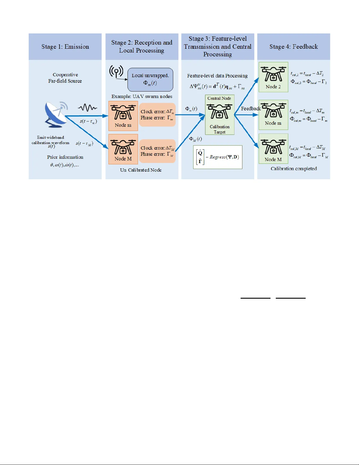
1 Joint T ime–Phase Synchronization for Distrib uted Sensing Networks via Feature-Le vel Hyper -Plane Regression Kailun T ian, Kaili Jiang, Dechang W ang, Y uxin Zhao, Y uxin Shang, Hancong Feng and Bin T ang Abstract —Achieving coherent integration in distributed In- ternet of Things (IoT) sensing networks requir es precise syn- chronization to jointly compensate clock offsets and radio- frequency (RF) phase errors. Con ventional two-step protocols suffer from time–phase coupling, where residual timing offsets degrade phase coherence. This paper proposes a generalized hyper -plane regr ession (GHR) framework for joint calibration by transforming coupled spatiotemporal phase evolution into a unified regr ession model, enabling effective parameter de- coupling. T o support resour ce-constrained IoT edge nodes, a feature-le vel distributed ar chitecture is dev eloped. By adopting a linear frequency-modulated (LFM) wa vef orm, the model order is r educed, yielding linear computational complexity . In addition, a unidirectional featur e transmission mechanism eliminates the communication overhead of bidirectional timestamp exchange, making the approach suitable f or resource-constrained IoT net- works. Simulation results demonstrate r eliable picosecond-level synchronization accuracy under sever e noise across kilometer- scale distributed IoT sensing networks. Index T erms —Internet of Things (IoT), distributed coher ent system, manifold geometry , joint time-phase calibration. I . I N T RO D U C T I O N D ISTRIBUTED coherent sensing networks, such as coop- erativ e uncre wed aerial vehicle (U A V) swarms [1], [2] and wireless edge sensor networks [3], [4], have emerged as a transformativ e paradigm in the modern Internet of Things (IoT) [5]. By coherently integrating spatially distributed nodes into a virtual large-scale aperture, these architectures enable scalable network-le vel sensing and enhanced coherent pro- cessing capability [6]. Howe ver , realizing the full potential of coherent integration demands extreme synchronization across the entire network [7]. Unlike traditional monolithic arrays tethered by rigid hardware backplanes [8], distributed IoT nodes are entirely wireless [9], relying on independent lo- cal oscillators and radio-frequency (RF) front-ends. Conse- quently , synchronization imperfections inherently manifest at two distinct physical lev els: the macroscopic clock synchro- nization error representing the absolute timestamp offset in the nanosecond re gime, and the microscopic RF initial phase error representing the fractional wav elength mismatch [10]. Achieving precise and joint calibration of these spatiotemporal parameters remains a critical bottleneck in deploying macro- scopic IoT sensing clusters. This work was supported in part by the National Natural Science Foundation of China under Grant 62301119. (Corresponding author: Kaili Jiang.) Kailun T ian, Kaili Jiang, Dechang W ang, Y uxin Zhao, Y uxin Shang, Hancong Feng and Bin T ang are with the Univ ersity of Electronic Science and T echnology of China, Chengdu, Sichuan, 611731, China (e-mail: kailun tian@163.com; jiangkelly@uestc.edu.cn; c13844033835@163.com; 1051172535@qq.com; 202411012307@std.uestc.edu.cn; 2927282941@qq.com; bint@uestc.edu.cn). T o address these synchronization challenges, extensi ve re- search has been conducted [11]. Packet-based protocols op- erating at the MAC or network layer , such as the Precision T ime Protocol (PTP), Network Time Protocol (NTP), and var - ious broadcast-based reference schemes [12], [13], are widely adopted in standard wireless networks. Building upon these, numerous closed-loop T wo-W ay Message Exchange (TWME) and consensus-based algorithms have been proposed to jointly estimate clock ske w , of fset, and dynamic delays [14]–[17]. While these protocols can achieve microsecond to nanosecond clock alignment, they fundamentally rely on frequent, bidirec- tional packet handshakes. This paradigm consumes massiv e communication bandwidth, introduces highly random MA C- layer queuing delays, and completely ignores the RF phase. T o mitigate these communication o verheads and en vironmental constraints, approaches like partial timestamp exchange mech- anisms [18] hav e been explored. Alternati vely , physical-layer algorithms—utilizing techniques lik e pulse-coupled oscilla- tors and unsupervised deep-learning-assisted synchronization [19]—hav e successfully bypassed MAC-layer uncertainties, pushing temporal accuracy into the sub-nanosecond regime. Nev ertheless, existing methodologies almost univ ersally adopt a separated two-step calibration paradigm, in which macro- scopic clock delays are first estimated, follo wed by phase com- pensation based on the estimated delays [10]. This sequential strategy becomes unreliable in the microw av e regime, where ev en picosecond-le vel residual timing errors are significantly amplified by high-frequency carriers, leading to sev ere phase distortion and degraded coherent processing performance [20]. In many practical IoT applications, synchronization re- quirements become the primary bottleneck for system de- ployment [21]. In such cases, the associated computational cost, power consumption, and implementation complexity of synchronization may even exceed those of the sensing task itself. Meanwhile, the miniaturization trend of distributed IoT sensing nodes imposes stringent constraints on computa- tional resources [22], making high-complexity synchronization schemes impractical for edge deployment. Therefore, it is essential to dev elop a robust and low-complexity joint syn- chronization framew ork that enables orthogonal decoupling of macroscopic time delays and microscopic spatial phase errors. Recently , the Dynamic Manifold theory was introduced, providing a promising geometric perspectiv e for analyzing distributed large-aperture arrays [23]. By exploiting the kine- matic ev olution of non-stationary broadband signals, this the- ory re veals that under non-negligible macroscopic apertures, the high-order expansion of the dynamic generator intensely couples with large spatial delays. This dynamic coupling forcefully twists the manifold trajectory into a highly complex 2 curve. While e xisting studies ha ve successfully utilized the intrinsic geometric features (e.g., curv ature) of this twisted manifold to resist microscopic RF phase errors, they face two critical gaps when applied to distrib uted IoT synchroniza- tion. First, they exclusiv ely focus on spatial phase ambiguity , completely neglecting the macroscopic clock synchronization offsets. Second, directly extracting parameters from this exact high-dimensional manifold requires multiv ariate matrix pseu- doin verse operations and high-order numerical differentiation. This imposes a prohibitiv e computational burden, strictly limiting its practical deployment on resource-constrained IoT edge nodes. T o bridge this critical theoretical and engineering gap, this paper proposes a Generalized Hyper-plane Regression (GHR) calibration framework customized for distributed IoT networks. Instead of relying on static spatial snapshots, we systematically establish the e xact high-dimensional topological mapping of the dynamic hyper -plane. By formulating this high-order geometric transformation as a multi variate ma- trix re gression model, the highly nonlinear space-time-phase coupling problem is translated into a tractable mathematical framew ork, allo wing for the analytical embedding and or- thogonal decoupling of both macroscopic clock errors and microscopic phase errors. Building upon this generalized geometric foundation, we dev elop a targeted feature-level distributed synchronization ar- chitecture to guarantee practical IoT deployment. By strategi- cally selecting the Linear Frequency Modulated (LFM) signal as the cooperativ e calibration source, the dynamic order of the framework is strictly truncated. W e mathematically prove that this specific dynamic selection forces the computationally expensi ve multidimensional hyper-plane to elegantly collapse back into a 2D hyper-line, plummeting the algorithmic com- putational complexity to a strict linear order . Operating ov er a passi ve feature-le vel interaction mechanism, the distrib uted nodes unidirectionally transmit highly compressed 1D phase trajectories. This architectural inno vation eliminates the com- munication overhead and queuing uncertainties inherent in bidirectional MA C-layer timestamp exchanges, successfully breaking the error floor of con ventional two-step schemes to achiev e robust, closed-form picosecond-level synchronization across macroscopic IoT apertures. The remainder of this paper is organized as follows. Section II establishes the distributed signal model and formulates the fatal time-phase coupling dilemma. Section III systemati- cally dev elops the generalized dynamic hyper-plane geometry and the orthogonal decoupling mechanism under macroscopic apertures. Section IV details the feature-le vel distrib uted cal- ibration architecture, the GHR algorithm, and the theoretical operating boundaries. Section V presents comprehensiv e ex- perimental results to e valuate the proposed frame work. Finally , Section VI concludes the paper . I I . D I S T R I B U T E D S I G NA L M O D E L A N D S M A L L - A P E RT U R E H Y P E R - L I N E G E O M E T RY A. Distributed Observation Model and T ime-Phase Coupling Dilemma Consider a cooperativ e far-field source broadcasting a wide- band non-stationary signal to a distributed IoT sensing net- work. Let the analytic representation of the source signal be denoted by s ( t ) = exp( j Φ( t )) , where Φ( t ) characterizes the total instantaneous phase. The instantaneous frequenc y of the source is defined as the first-order time deriv ativ e of the phase: ω ( t ) = d Φ( t ) dt = ˙ Φ( t ) (1) Assume a distributed coherent IoT sensing network consist- ing of M spatially separated receiving nodes (e.g., uncrewed aerial vehicles or wireless edge sensors). W e designate the first node ( m = 1 ) as the absolute spatio-temporal reference origin. For the m -th distributed node, let τ m ( θ ) denote the spatial propagation delay determined by the Direction of Arriv al (DO A) θ and the distrib uted node geometry . In such untethered distributed IoT architectures, the inde- pendent local oscillators of the receiving edge nodes cannot achiev e perfect synchronization. These inherent synchroniza- tion imperfections introduce two distinct levels of error: 1) Macroscopic Clock Synchronization Error ( ∆ T m ): Representing the absolute time-stamp offset in the nanosecond regime. 2) Microscopic RF Phase Error ( Γ m ): Representing the initial phase mismatch in the radio frequency (RF) front- end, where Γ m ∈ [ − π , π ) . Consequently , the observ ation signal receiv ed at the m -th IoT node is a delayed and phase-rotated version of the source signal, strictly formulated as: x m ( t ) = exp  j  Φ( t − τ m ( θ ) − ∆ T m ) + Γ m   + n m ( t ) (2) where n m ( t ) is the additive white Gaussian noise (A WGN). The distrib uted observation vector can be compactly written as x ( t ) = [ x 1 ( t ) , x 2 ( t ) , . . . , x M ( t )] T ∈ C M . Under this mathematical model, any coherent processing of the signal across the IoT network must address the joint compensation of clock synchronization errors and phase er- rors. Since Φ( t ) encompasses both the high-frequency car- rier and the wideband modulation, any residual error δ T in estimating the macroscopic clock delay ∆ T m will translate into a massi ve, time-v arying phase rotation ω ( t ) δ T . This coupling completely randomizes the subsequent estimation of the microscopic phase Γ m , dictating that the temporal delay ( τ m + ∆ T m ) and the spatial phase ( Γ m ) must be orthogonally decoupled within a joint estimation frame work. B. Dynamic Manifold and Small-Apertur e Hyper-line Geom- etry T o ov ercome the static ambiguity formulated in Section II-A, we must abandon the traditional paradigm of treating the time-varying observation x ( t ) as a collection of isolated static snapshots. Instead, by exploiting the continuous temporal 3 ev olution of the non-stationary signal, we model x ( t ) as a smooth, parameterized trajectory tracing a dynamic manifold M in the high-dimensional complex space C M [23]. The local geometric ev olution of this manifold is funda- mentally characterized by its first-order kinematic deriv ati ve, i.e., the tangent vector v ( t ) = ˙ x ( t ) . Applying the chain rule to the noise-free component of the observation model (2), the element-wise deriv ative for the m -th sensor yields: v m ( t ) = ˙ Φ( t − τ m ( θ ) − ∆ T m ) x m ( t ) (3) Recalling the definition of instantaneous frequency ω ( t ) = ˙ Φ( t ) , the complete tangent vector can be elegantly formulated using a diagonal operator matrix: v ( t ) = Ω ( θ , t ) x ( t ) (4) where Ω ( θ , t ) is the Dynamic Generator , defined as the instantaneous diagonal frequency matrix diag ( j ω ( t − τ tot, 1 ) , . . . , j ω ( t − τ tot,M )) , with τ tot,m = τ m ( θ ) + ∆ T m representing the total macroscopic delay . Equation (4) re veals a profound physical insight: the spatial ev olution of the array manifold is strictly driven by the tempo- ral dynamics of the source signal. For traditional microscopic arrays, the delay is negligible, and Ω trivially de generates to a scalar matrix j ω ( t ) I . Howe ver , in modern distributed sensing networks, the macroscopic spatial separation between nodes, coupled with substantial initial clock synchronization errors, can result in total delays τ tot,m reaching hundreds of nanoseconds. Under such macroscopic scales, the dynamic generator must be expanded using its high-order T aylor series: ω ( t − τ tot,m ) = ω ( t ) − ˙ ω ( t ) τ tot,m + 1 2 ¨ ω ( t ) τ 2 tot,m − . . . (5) Substituting (5) back into the e volution model, it becomes evident that the high-order temporal dynamics of the signal (e.g., ˙ ω ( t ) and ¨ ω ( t ) ) explicitly couple with the large delays, acting as se vere geometric perturbations. The unknown space- time parameters (DOA θ and clock offset ∆ T m ) are deter- ministically embedded within the coefficients of these high- order dynamic terms, while the microscopic phase error Γ m is independently isolated as a spatial constant in x ( t ) . This kinematic analysis demonstrates that the entangled Space-T ime-Phase parameters are systematically encoded within the continuous, high-order ev olution of the dynamic manifold. Motiv ated by this geometric perspecti ve, Chapter 3 will systematically reconstruct this high-dimensional topo- logical mapping and propose the Generalized Hyper-plane Regression framework, aiming to analytically flatten this com- plex trajectory and achiev e exact orthogonal decoupling of all parameters. I I I . G E N E R A L I Z E D D Y N A M I C G E O M E T RY A N D H Y P E R - P L A N E R E G R E S S I O N A L G O R I T H M A. The Dynamic Hyper-plane As established in the kinematic analysis of Section II and the previous work [23], the spatial phase differences extracted from the zero-order dynamic manifold x ( t ) and its first- order tangent vector v ( t ) e xplicitly encapsulate the high-order structural characteristics of the dynamic generator . Note that in Eq. (4), the tangent vector v ( t ) introduces a constant phase shift ( ∠ j = π / 2 ) and a frequency-dependent amplitude mapping. Since the instantaneous frequency is strictly positive ( ∠ ω ( t ) ≡ 0 ), this deri vati ve-induced phase shift perfectly vanishes via common-mode cancellation when extracting the relativ e spatial phase dif ferences between nodes. By retaining all high-order terms of the T aylor expansion for the delayed instantaneous phase Φ( t − τ tot,m ) , the e xpansion yields: ∆Ψ x m ( t ) = ∆Ψ v m ( t ) = ∞ X k =1 ( − τ tot,m ) k k ! ω ( k − 1) ( t ) + Γ m (6) Equation (6) rev eals a profound topological transforma- tion that directly reflects the kinematic expansion of the dynamic generator . Under macroscopic apertures, the high- order temporal dynamics of the signal—specifically the chirp rate ˙ ω ( t ) , the jerk ¨ ω ( t ) , and be yond—intensely couple with the large spatial delays, acting as severe geometric perturbations. By conceptualizing these continuously time-varying dynamic variables [ ω ( t ) , ˙ ω ( t ) , ¨ ω ( t ) , . . . ] as independent coordinate axes in a high-dimensional parameter space, the twisted complex manifold deterministically flattens onto a generalized Dynamic Hyper-plane . Mathematically , the generalized dynamic Hyper-plane can be compactly rewritten as a generalized linear observation model: ∆Ψ x m ( t ) = ∆Ψ v m ( t ) = d T ( t ) q m + Γ m (7) where the time-varying Dynamic Basis V ector d ( t ) and the time-in variant Geometric P arameter V ector q m for the m -th node are defined as: d ( t ) =  − ω ( t ) , 1 2 ˙ ω ( t ) , − 1 6 ¨ ω ( t ) , . . .  T (8) q m =  τ tot,m , τ 2 tot,m , τ 3 tot,m , . . .  T (9) This formulation establishes a uni versal parameter estima- tion framew ork for the dynamic manifold. The continuous dynamics d ( t ) explicitly serve as the known non-stationary basis spanning the Hyper-plane subspace, while the macro- scopic spatial delays and microscopic phase errors are strictly localized within the constant projection vector q m and the intercept Γ m , respecti vely . Consequently , the highly nonlinear Space-T ime-Phase coupling problem is formally transformed into a tractable multidimensional linear re gression task:  ˆ Q ˆ Γ  = Regress ( Ψ , D ) (10) The solvability and complexity of this regression strictly depend on the effecti ve dimensionality (i.e., the number of non-zero time-varying components) of the dynamic basis d ( t ) . B. Generalized Hyper-plane Re gr ession Algorithm T o accommodate arbitrary non-stationary signals containing high-order dynamic deri vati ves, we construct a generalized high-dimensional linear re gression model, termed the Gener- alized Hyper-plane Re gression . 4 Suppose the processing center gathers continuous valid snapshots o ver K discrete time indices { t 1 , t 2 , . . . , t K } . F or the m -th distributed node relati ve to the reference node, we define the observation vector ψ m ∈ R K × 1 as: ψ m = [∆Ψ v m ( t 1 ) , ∆Ψ v m ( t 2 ) , . . . , ∆Ψ v m ( t K )] T (11) T o process all M − 1 uncalibrated nodes simultaneously , we construct the global phase observation matrix Ψ = [ ψ 2 , ψ 3 , . . . , ψ M ] ∈ R K × ( M − 1) . According to the analytical model in (7), we stack the time- varying dynamic basis vector d ( t ) ∈ R d × 1 (where d is the dynamic order of the signal) across the K snapshots to form the known Dynamic Basis Matrix D ∈ R K × d : D = [ d ( t 1 ) , d ( t 2 ) , . . . , d ( t K )] T (12) Similarly , we construct the global Geometric Parameter Matrix Q ∈ R d × ( M − 1) containing the unknown high-order macro- scopic delay terms, and the phase error vector Γ ∈ R 1 × ( M − 1) : Q = [ q 2 , q 3 , . . . , q M ] (13) Γ = [Γ 2 , Γ 3 , . . . , Γ M ] (14) The generalized dynamic Hyper -plane decoupling problem is therefore strictly formulated as a multiv ariate matrix regres- sion equation: Ψ = DQ + 1 K Γ + N Ψ (15) where 1 K is a K × 1 vector of ones, and N Ψ represents the residual Gaussian noise matrix in the phase parameter space. T o decouple the structural geometric matrix Q from the intercept vector Γ , we apply the centering projection operator P c = I K − 1 K 1 K 1 T K to both sides of the equation. This yields the mean-centered matrices ¯ Ψ = P c Ψ and ¯ D = P c D , effecti vely eliminating the intercept term: ¯ Ψ = ¯ DQ + P c N Ψ (16) By utilizing the Ordinary Least Squares (OLS) or Principal Component Analysis (PCA) frame work, the optimal estimate for the geometric parameter matrix ˆ Q is derived: ˆ Q = ( ¯ D T ¯ D ) − 1 ¯ D T ¯ Ψ (17) Subsequently , the uncalibrated initial phase error v ector ˆ Γ is perfectly retrie ved by substituting ˆ Q back into the centroid of the original observation: ˆ Γ = 1 K 1 T K  Ψ − D ˆ Q  (18) Finally , recognizing that the first row of ˆ Q solely contains the first-order total macroscopic delay terms τ tot,m = τ m ( θ ) + ∆ T m , the clock synchronization error ∆ T m can be explicitly decoupled giv en the spatial geometry τ m ( θ ) . The complete ex ecution flow is summarized in Algorithm 1. Algorithm 1 The GHR Algorithm Input: { ψ m } M m =2 , D and τ ( θ ) . Output: { ∆ ˆ T m } M m =2 and { ˆ Γ m } M m =2 . 1: Ψ = [ ψ 2 , ψ 3 , . . . , ψ M ] . 2: P c = I K − 1 K 1 K 1 T K . 3: Centralize matrices: ¯ Ψ ← P c Ψ and ¯ D ← P c D . 4: ˆ Q ← ( ¯ D T ¯ D ) − 1 ¯ D T ¯ Ψ . 5: ˆ Γ ← 1 K 1 T K ( Ψ − D ˆ Q ) . 6: ˆ τ tot ← ˆ Q (1 , :) . 7: for m = 2 to M do 8: Decouple clock error: ∆ ˆ T m ← ˆ τ tot,m − τ m ( θ ) . 9: Map RF phase error to principal branch [ − π, π ) : ˆ Γ m ← wrapT oPi ( ˆ Γ m ) . 10: end f or 11: return { ∆ ˆ T m } M m =2 and { ˆ Γ m } M m =2 . I V . D I S T R I B U T E D G H R C A L I B R A T I O N F R A M E W O R K A N D P E R F O R M A N C E B O U N D A R I E S Building upon the rigorous mathematical foundation of the GHR algorithm derived in Section III, this section translates the pure multidimensional regression theory into a highly efficient, practical distributed engineering protocol tailored for IoT applications. W e propose a passiv e feature-lev el interac- tion architecture, explicitly introduce a dimensionality reduc- tion mechanism to resolve algorithmic complexity bottlenecks on resource-constrained edge devices, and rigorously analyze the fundamental physical boundaries governing the system’ s performance. A. Distributed F eatur e-Level Interaction Arc hitectur e T raditional distributed synchronization protocols, such as T wo-W ay Message Exchange (TWME), fundamentally rely on the bidirectional transmission of discrete MA C-layer pack- ets to extract timestamps. This paradigm consumes massive communication bandwidth, introduces highly random queuing delays, and severely compromises the energy efficienc y and electromagnetic stealth of non-cooperativ e sensing clusters like U A V swarms and wireless edge sensors. T o overcome these bottlenecks, Fig. 1 illustrates the overall implementation architecture of the proposed distributed GHR calibration frame work, which adheres to a strict feature-lev el interaction paradigm designed for low-bandwidth IoT en viron- ments. In the first stage, a known wideband calibration wav eform is broadcast by a far-field cooperative source with a prior angle of arriv al θ . Each distributed IoT node captures this signal and performs robust local processing to extract the unwrapped spatial phase trajectory . It is worth noting that, although the phase of x can be directly extracted using a single antenna at each node, such estimation is highly susceptible to noise in practical scenarios. T o enable robust local phase e xtraction, we adv ocate equipping each node with a subarray and performing local processing based on subarray-level tangent vectors v , which significantly enhances system robustness. 5 Fig. 1. Architecture of the proposed feature-lev el cooperativ e calibration framework in a distributed IoT sensing network. Subsequently , in Stage 3, instead of transmitting gigabytes of raw RF baseband data, each uncalibrated edge node for- wards only its one-dimensional, highly compressed feature- lev el data vector , ψ m , to a central data processing node via a unidirectional link. Finally , the central node constructs the gathered phase matrix Ψ and utilizes the GHR algorithm to jointly and orthogonally decouple the clock and RF phase errors, feeding them back to precisely calibrate the distributed swarm. This architecture thoroughly eliminates the need for bidi- rectional pack et e xchanges, bypassing MA C-layer queuing uncertainties while ensuring a kilobyte-lev el communication footprint. B. Algorithmic Comple xity and Dimensionality Reduction While the GHR frame work provides a universal mathe- matical model capable of handling arbitrary dynamic orders ( d ≥ 1 ), performing multidimensional matrix operations poses a se vere computational bottleneck for resource-constrained IoT edge networks. Specifically , the computational complexity of the centralized GHR algorithm is e xclusiv ely dominated by the pseudoin verse and matrix multiplications. For M − 1 uncali- brated nodes, K valid temporal snapshots, and a source signal with dynamic order d , computing the cov ariance matrix ¯ D T ¯ D requires O ( K d 2 ) floating-point operations. The subsequent matrix in version requires O ( d 3 ) operations, and the cross- correlation projection ¯ D T ¯ Ψ requires O ( K dM ) operations. Thus, the o verall computational complexity scales as O ( K d 2 + d 3 + K dM ) . For highly non-stationary signals with large dynamic orders, extracting errors from high-dimensional hyper-planes inherently imposes a heavy computational bur- den, threatening the real-time responsi veness and battery life of IoT nodes. T o guarantee real-time engineering feasibility , we strate- gically select the LFM signal as the cooperative calibration source. For an LFM signal, the chirp rate is a known constant ( ˙ ω ( t ) = 2 π µ ), and all higher-order deriv ati ves identically vanish ( ¨ ω ( t ) = 0 ). This specific dynamic condition enforces a strict truncation of the dynamic order to d = 1 . Most cru- cially , because ˙ ω ( t ) is constant, the second-order perturbation term ceases to be a time-v arying coordinate axis, collapsing into a deterministic scalar . The multidimensional Hyper-plane precisely degenerates into a 2D Hyper-line: ∆Ψ v m ( t ) = − ( τ m ( θ ) + ∆ T m ) ω ( t ) + h Γ m + π µ ( τ m ( θ ) + ∆ T m ) 2 i | {z } Generalized Intercept ˜ Γ m (19) Algorithmically , this deliberate selection allows the dynamic basis matrix D to collapse into a single-column instantaneous frequency vector . The computationally expensi ve d × d matrix in version gracefully degenerates into a trivial scalar di vision requiring merely O (1) operations. Correspondingly , the over - all computational complexity of the decoupling algorithm plummets to a strict linear order of O ( K M ) . By dri ving the computational overhead to its theoretical minimum, the LFM-based framew ork guarantees robust execution e ven for massiv e-scale distrib uted IoT sensing clusters. C. Theoretical Operating Boundaries The validity of the proposed framew ork is governed by two fundamental physical boundaries: the algorithmic phase Nyquist limit and the (signal-to-noise ratio) SNR threshold. The phase unwrapping operation inherently requires that the phase variation between adjacent discrete samples does not exceed ± π . For a signal with bandwidth B and pulse 6 duration T dur , the maximum frequency variation per sample (at sampling rate f s ) is ∆ f = B / ( T dur f s ) . The corresponding maximum phase increment induced by a macroscopic delay τ max is ∆ ϕ = 2 π ∆ f · τ max . T o av oid catastrophic cycle slips along the temporal axis, we must satisfy ∆ ϕ ≤ π . This establishes the rigorous maximum unambiguous macroscopic aperture bound: D max = c · τ max ≤ c · f s · T dur 2 B (20) This theoretical boundary mathematically guarantees that higher sampling rates or extended pulse durations linearly expand the resolvable macroscopic distance, ensuring the algorithm’ s compatibility with kilometer-scale distributed IoT networks. In addition, the fundamental constraint of the proposed decoupling algorithm lies in the non-linear phase unwrapping process, where se vere noise can induce catastrophic phase jumps (i.e., cycle slips), destroying the topological structure of the e xtracted hyper -plane. Although the cooperativ e calibration signal typically guarantees a relativ ely high SNR, inv estigat- ing the frame work’ s performance under lo w-SNR conditions remains practically meaningful for resource-constrained edge nodes. T o ov ercome this threshold, introducing a local sub-array at each distrib uted node is highly advocated. For example, the local processing module can perform coherent integration ov er the sub-array observations, which significantly enhances the anti-noise capability during local phase extraction. Con- sequently , as long as the post-integration SNR stays above the phase wrapping threshold, the generalized hyper -plane decoupling remains strictly valid. T o v alidate this mechanism, the experimental section of this paper explicitly compares the performance disparity between directly extracting the phase of x (using a single antenna) and emplo ying the local sub-array processing ( v ), decisively demonstrating the framew ork’ s ca- pability to reliably operate in severely degraded environments. The local processing module lev erages techniques like Sin- gular V alue Decomposition to perform coherent integration ov er a sliding window of length L . This optimal rank-1 projec- tion yields an asymptotic processing gain of 10 log 10 ( L ) dB. The generalized hyper-plane decoupling remains v alid as long as the post-integration SNR stays above the non-linear phase unwrapping threshold. Consequently , the minimum required SNR follo ws a phase transition behavior . While an enlarged distributed aperture necessitates higher geometric stability , the substantial integration gain allows the proposed framew ork to reliably operate in sev erely degraded en vironments (e.g., 0 dB), decisiv ely breaking the performance floor of con ventional packet-based synchronization protocols. V . E X P E R I M E N TA L R E S U L T S A. Experiment 1: High-Order Manifold T opology and Multi- dimensional Hyper-plane V alidation This experiment aims to verify the correctness of the geom- etry of dynamic manifold hyperplanes on a large, distrib uted scale. For the distrib uted receiver nodes, the sampling rate is set to 5 GHz. The system consists of two distributed 1.9 2 2.1 2.2 2.3 2.4 2.5 2.6 Instantaneous Frequency (GHz) -300 -250 -200 -150 -100 -50 0 Unwrapped Phase Diff (rad) Extracted Phase Trajectory Exact Theoretical Model (a) LFM signal. 1.7 1.8 1.9 2 2.1 2.2 2.3 Instantaneous Frequency (GHz) -50 0 50 100 150 200 250 300 Unwrapped Phase Diff (rad) Extracted Phase Trajectory Exact Theoretical Model (b) SFM signal. 1.9 2 2.1 2.2 2.3 2.4 2.5 2.6 Instantaneous Frequency (GHz) -250 -200 -150 -100 -50 0 Unwrapped Phase Diff (rad) Extracted Phase Trajectory Exact Theoretical Model (c) QFM signal. 1.7 1.8 1.9 2 2.1 2.2 2.3 Instantaneous Frequency (GHz) -50 0 50 100 150 200 250 300 350 Unwrapped Phase Diff (rad) Extracted Phase Clusters Exact Theoretical Model (d) 2FSK signal. Fig. 2. High-order manifold topology of far-field transmitting node signal. 1000 -2000 0 -1500 1 Chirp Rate (MHz/us) 500 F requency (G Hz ) -1000 Phase Diff (rad) 2 -500 0 3 0 3D Regression Hyper-plane Extracted Spatial Trajectory True Phase Error ! (1.234 rad) Intercept axis Fig. 3. Multidimensional Hyper-plane of QFM signal. nodes separated by a macroscopic distance of approximately 30 meters. The uncalibrated node is injected with a clock synchronization error of 3 . 45 ns and an RF initial phase error of 1 . 234 rad. For the far-field transmitting node, the carrier frequency is 2 GHz, the signal pulse width is 1 µ s, and the bandwidth is unified to 500 MHz. Four typical signal types are ev aluated: a LFM signal, a Sinusoidal Frequency Modulated (SFM) signal with a modulation rate of 2 MHz, a Quadratic Frequenc y Modulated (QFM) signal, and a 2-le vel Frequency-Shift Ke ying (2FSK) signal with a symbol rate of 10 MBaud. T o isolate the pure geometric morphology from receiv er thermal noise, a SNR of 50 dB is applied. Fig. 2 illustrates the geometric topologies of the four signals projected onto the two-dimensional instantaneous frequency versus unwrapped phase difference plane. Under a traditional microscopic array aperture, the second-order delay residuals approach zero, and the phase evolution of all signals presents as a straight line. Howe ver , under the macroscopic distributed aperture, the high-order dynamics of the signals explicitly 7 reshape the topological structure of the two-dimensional pro- jection. Since the instantaneous chirp rate of the LFM signal is constant, its second-order residual degenerates into a fixed intercept shift, maintaining a one-dimensional line morphol- ogy , as shown in Fig. 2(a). In contrast, as shown in Fig. 2(b), the oscillating chirp rate of the SFM signal distorts its two-dimensional projection into a closed Lissajous ellipse, the linearly v arying chirp rate of the QFM signal transforms its projection into a parabola, and the discrete frequency hopping of the 2FSK signal manifests as separated data clusters, as shown in Fig. 2(c) and 2(d). The exact high-order theoretical analytical curves match the extracted observation point clouds, confirming that the macroscopic aperture amplifies the non- linear coupling of high-order dynamics, which in validates the two-dimensional linear model for signals with non-constant chirp rates. Fig. 3 demonstrates the three-dimensional hyper-plane geo- metric characteristics of the QFM signal. By expanding the observation phase space to a three-dimensional parameter space including instantaneous frequency and instantaneous chirp rate, the curve that projected in the two-dimensional plane is flattened onto a tilted dynamic hyper -plane. Ex- trapolating this three-dimensional hyper-plane towards zero frequency and zero chirp rate yields an intercept on the v ertical axis that matches the pre-set true RF initial phase error . The estimated clock synchronization error is 3 . 4508 ns, with a calibration accuracy of 7 . 9863 × 10 − 4 ns. The estimated phase error is − 1 . 8966 rad, with a calibration error of 3 . 1306 rad. This demonstrates that constructing a multiv ariate dynamic linear regression model by introducing the chirp rate as an independent variable can absorb the high-order ev olution non- linearity of complex signals, achie ving topological flattening and orthogonal decoupling of the macroscopic clock and microscopic RF initial phase. B. Experiment 2: The GHR Algorithm Under LFM Signal This experiment aims to verify that, when an LFM signal is employed as the calibration signal, the GHR algorithm can be reformulated as a re gression problem over a multi- dimensional hyper-linear geometric structure, and to further demonstrate that equipping each node with a subarray can provide significant performance gains compared to a single- antenna configuration. For a distributed system, the sampling rate of each node is set to 5 GHz. The system consists of three distrib uted nodes, where the first node serves as the reference, and the subsequent nodes are separated by macroscopic distances corresponding to relati ve propagation delays of 15 ns and 25 ns. The clock synchronization errors are set to 3 . 45 ns and − 2 . 15 ns, and the phase errors are 1 . 234 rad and − 0 . 876 rad. T o provide a comparati ve ablation analysis, the nodes are alternately configured with a sub-array of 4 antennas spaced at half- wa velength and a degraded single-antenna setup. For the far - field transmitting node, the calibration source emits an LFM signal. The carrier frequency is 2 GHz, the signal pulse width is 1 µ s, and the bandwidth is 500 MHz. The SNR is set to 5 dB. 0 -10 -20 " * 2,1 (rad) -80 -30 -60 2.1 Frequency (GHz) -40 2.2 -40 " * 3,1 (rad) 2.3 -20 2.4 -50 0 20 0.1 0.2 0.3 0.4 0.5 0.6 0.7 0.8 0.9 Time ( 7 s) Extracted Spatial Phase Trajectory Fitted 3D Hyper-line Fig. 4. 3D Hyper-line Geometry . 0 0.5 1 1.5 2 Instantaneous Frequency (GHz) -50 0 50 100 150 200 250 300 Unwrapped Phase Difference (rad) Node 2 Data Node 2 Fit Node 3 Data Node 3 Fit Intercept axis (a) 2D projection using four antennas. 0 0.5 1 1.5 2 Instantaneous Frequency (GHz) -50 0 50 100 150 200 250 300 Unwrapped Phase Difference (rad) Node 2 Data Node 2 Fit Node 3 Data Node 3 Fit Intercept axis (b) 2D projection using a single an- tenna. Fig. 5. A visual comparison of multi-antenna node’ s noise-canceling capa- bilities. Fig. 4 illustrates the three-dimensional hyper-line geometry of the three distributed nodes. By extracting the unwrapped spatial phase differences relative to the reference node, the time-ev olving dynamic manifold collapses into a structured one-dimensional straight line in the three-dimensional param- eter space composed of the instantaneous frequenc y and dual phase differences. Fig. 5(a) presents the two-dimensional projection of the phase differences for the two uncalibrated nodes under the four-antenna configuration at 5 dB SNR. Supported by the local coherent integration of the multi-antenna node, the un- wrapped phase trajectories form continuous point clouds that adhere to the theoretical hyper-line model, enabling parameter decoupling. Quantitativ e analysis of the four-antenna configu- ration reveals accurate clock error decoupling. For Node 2, the estimated clock error is 3 . 4474 ns compared to the true value of 3 . 4500 ns (an error of 2 . 61 × 10 − 3 ns), and the estimated phase error is − 1 . 9458 rad compared to the true 1 . 2340 rad (an error of 3 . 18 rad). For Node 3, the estimated clock error is − 2 . 1502 ns compared to the true − 2 . 1500 ns (an error of 1 . 71 × 10 − 4 ns), and the estimated phase error is 2 . 2622 rad compared to the true − 0 . 8760 rad (an error of 3 . 14 rad). Fig. 5(b) depicts the two-dimensional projection under the single-antenna degradation. Lacking the noise suppression, direct phase unwrapping suffers from cycle slips, causing the point clouds to fracture and div erge significantly from the theoretical linear trend. Consequently , the single-antenna quantitativ e results deteriorate drastically . For Node 2, the 8 0 1 2 3 4 5 6 7 Distributed Aperture Distance (km) 10 -5 10 0 10 5 RMSE of " T (ns) 0.6 km 1.5 km 6.0 km f s = 2 GHz f s = 5 GHz f s = 20 GHz Fig. 6. The effect of node sampling rate on distributed effecti ve aperture. estimated clock error is − 1 . 0615 ns (an error of 4 . 51 ns) and the estimated phase error is 1 . 6860 rad (an error of 4 . 52 × 10 − 1 rad). For Node 3, the estimated clock error col- lapses to − 7 . 8045 ns (an error of 5 . 65 ns) and the estimated phase error is 0 . 4906 rad (an error of 1 . 37 rad). Evidently , the greater the number of distributed node’ s internal array elements, the stronger the anti-noise capability . C. Experiment 3: V alidation of Effective Distance for Dis- tributed Nodes This experiment aims to validate the ef fective macroscopic distance between distrib uted nodes supported by the GHR and analyzes how system parameters influence this operating boundary . For the distributed recei ver network, the baseband sampling rate is configured as a variable parameter , tested at 2 GHz, 5 GHz, and 20 GHz. The macroscopic distance be- tween distributed nodes are scanned from 0 . 1 km up to 15 km. For the far-field transmitting node, the calibration source emits an LFM signal. The carrier frequency is 2 GHz. The signal pulse duration is tested at 1 µ s, 10 µ s, and 20 µ s. The signal bandwidth is ev aluated at 200 MHz, 500 MHz, and 800 MHz. The SNR is fixed at 30 dB to isolate the geometric phase collapse phenomenon from thermal noise interference. The experiment employs a control variable method across three sub-tests to independently e valuate the effects of sampling rate, pulse duration, and signal bandwidth on the maximum resolvable aperture. As illustrated in Fig. 6, the impact of the hardware sampling rate on the clock error estimation is significant. The root mean square error (RMSE) curves remain stable within the operational range but exhibit a vertical collapse exactly at the theoretical boundaries of 0 . 6 km, 1 . 5 km, and 6 . 0 km, confirming the analytical deriv ation of the phase Nyquist limit. Fig. 7 presents the influence of the signal pulse duration. The collapse points match the theoretical limits of 0 . 6 km, 6 . 0 km, and 12 . 0 km, verifying that extended signal durations proportionally expand the maximum unambiguous aperture. Fig. 8 demonstrates the ef fect of signal bandwidth, where the operational boundaries occur at 3 . 75 km, 1 . 50 km, and 0 . 94 km, showing an inv erse relationship with the bandwidth size. 0 2 4 6 8 10 12 14 Distributed Aperture Distance (km) 10 -5 10 0 10 5 RMSE of " T (ns) 0.6 km 6.0 km 12.0 km T dur = 1 7 s T dur = 10 7 s T dur = 20 7 s Fig. 7. The effect of broadcast node signal duration on distributed aperture. 0 1 2 3 4 5 Distributed Aperture Distance (km) 10 -5 10 0 10 5 RMSE of " T (ns) 3.75 km 1.50 km 0.94 km B = 200 MHz B = 500 MHz B = 800 MHz Fig. 8. The ef fect of broadcast node signal bandwidth on distributed aperture. In addition to the boundary v alidation, the results within the stable operational zones indicate a clear trend in estimation accuracy . Before reaching the phase collapse boundary , a higher sampling rate at the distrib uted nodes, a wider signal bandwidth, and a longer pulse duration from the transmitting node jointly contribute to a lower estimation error floor . Conclusiv ely , these findings demonstrate that by appropri- ately adjusting the system parameters, the proposed scheme can successfully accomplish rob ust clock synchronization for distributed nodes spanning several kilometers to tens of kilometers, effecti vely accommodating the scale of modern distributed sensing netw orks. D. Experiment 4: Impact of Distrib uted Apertur e Scale on Synchr onization Accuracy This experiment aims to in vestigate the impact of the macro- scopic distributed aperture size on the estimation accurac y of the clock error and RF initial phase, verifying the immunity of the GHR framework to inter-node distances within the effecti ve phase Nyquist boundary . For the distributed receiv er network, a baseband equiv alent model is employed with a sampling rate of 5 GHz. The network consists of a reference node and an uncalibrated node, alternately configured with a 4-element sub-array and a degraded single-antenna setup. The 9 -10 -5 0 5 10 15 20 Signal-to-Noise Ratio (dB) 10 -4 10 -2 10 0 10 2 10 4 RMSE of " T (ns) Theoretical CRB (4 antenna) " = = 100 ns (1 antenna) " = = 100 ns (4 antenna) " = = 500 ns (1 antenna) " = = 500 ns (4 antenna) " = = 1500 ns (1 antenna) " = = 1500 ns (4 antenna) (a) Time calibration RMSE. -10 -5 0 5 10 15 20 Signal-to-Noise Ratio (dB) 10 -1 10 0 10 1 10 2 RMSE of ! (Degree) Theoretical CRB (4 antenna) " = = 100 ns, (1 antenna) " = = 100 ns (4 antenna) " = = 500 ns, (1 antenna) " = = 500 ns (4 antenna) " = = 1500 ns, (1 antenna) " = = 1500 ns (4 antenna) (b) Phase calibration RMSE. Fig. 9. The effect of different spacing patterns within the effectiv e aperture on performance. macroscopic distance offsets between the nodes are ev aluated at three distinct levels: 100 ns, 500 ns, and 1500 ns, corre- sponding to approximate physical separations of 30 meters, 150 meters, and 450 meters. For the far-field transmitting node, the calibration source emits an LFM signal. The carrier frequency is 2 GHz, the signal pulse duration is 1 µ s, and the bandwidth is fix ed at 500 MHz. The SNR is swept from − 10 dB to 20 dB. At each SNR lev el, 100 independent Monte Carlo trials are performed to obtain statistically stable results. The simulation results present the RMSE of the clock and phase estimation alongside their corresponding theoretical Cram ´ er-Rao Bounds. Fig. 9(a) demonstrates that for the clock error estimation, the theoretical bounds and the proposed GHR curves for all three macroscopic apertures overlap perfectly . This confirms the mathematical deriv ation that the slope extraction accuracy is completely immune to the macroscopic distance between distributed nodes. Fig. 9(b) rev eals the phase error calibration performance. As the aperture scale increases, the second-order phase coupling induces a slight theoretical div ergence in the phase Cram ´ er-Rao Bounds. Nevertheless, the proposed GHR algorithm strictly tracks these diver ging theoretical limits without any performance degradation. In contrast, across both parameter estimations, the single-antenna scheme fails to achieve the theoretical bounds at low and mod- erate SNRs due to phase wrapping anomalies, emphasizing the necessity of local coherent integration regardless of the aperture scale. E. Experiment 5: Impact of Signal Bandwidth and Spatial Coher ence on Estimation Accur acy Building upon the conclusion from Experiment 4 that the macroscopic distance does not fundamentally constrain the synchronization accuracy within operational limits, this exper- iment fixes a relativ ely small aperture to inv estigate the impact of signal bandwidth and spatial coherence on the theoretical estimation limits. For the distributed receiv er network, the baseband sampling rate remains at 5 GHz. The macroscopic distance between the reference node and the uncalibrated node is fixed at approximately 3 meters. T o conduct an ablation study on spatial coherence, the distrib uted nodes are alternately configured with a 4-element sub-array and a degraded single-antenna setup. For the far-field transmitting node, the calibration source emits an LFM signal. The carrier frequency is 2 GHz, and the signal pulse duration is 1 µ s. -10 -5 0 5 10 15 20 Signal-to-Noise Ratio (dB) 10 -4 10 -2 10 0 10 2 RMSE of " T (ns) Theoretical CRB (4 antenna) B = 200 MHz (1 antenna) B = 200 MHz (4 antenna) B = 500 MHz (1 antenna) B = 500 MHz (4 antenna) B = 800 MHz (1 antenna) B = 800 MHz (4 antenna) (a) Time calibration RMSE. -10 -5 0 5 10 15 20 Signal-to-Noise Ratio (dB) 10 -1 10 0 10 1 10 2 10 3 RMSE of ! (Degree) Theoretical CRB (4 antenna) B = 200 MHz (1 antenna) B = 200 MHz (4 antenna) B = 500 MHz (1 antenna) B = 500 MHz (4 antenna) B = 800 MHz (1 antenna) B = 800 MHz (4 antenna) (b) Phase calibration RMSE. Fig. 10. The impact of bandwidth on performance. The signal bandwidth is e valuated at three distinct lev els: 200 MHz, 500 MHz, and 800 MHz. The SNR is swept from − 10 dB to 20 dB, with 100 independent Monte Carlo trials performed at each le vel. As shown in Fig. 10, the simulation results present the RMSE of the parameter estimation alongside their corre- sponding theoretical bounds under varying bandwidth con- ditions. As the signal bandwidth expands from 200 MHz to 800 MHz, the variance of the instantaneous frequency increases, which monotonically lo wers the theoretical bounds for both the clock and phase parameters, indicating that a larger bandwidth intrinsically provides stronger theoretical estimation capabilities. The proposed algorithm utilizing the 4-antenna strictly coincides with the theoretical bounds for both parameters, maintaining this optimal accuracy down to an SNR con ver gence threshold of approximately 4 dB. Con versely , the single-antenna exhibits degraded performance, with its con ver gence threshold delayed to 10 dB. Furthermore, ev en in the con verged high-SNR regime, the single-antenna scheme exhibits a consistent performance gap, yielding errors approximately half an order of magnitude higher than the multi-antenna-based bounds due to the absence of local spatial coherent integration gain. F . Experiment 6: Compr ehensive P erformance Comparison with T raditional Baselines This experiment comprehensively compares the proposed GHR framework with traditional baseline algorithms to e valu- ate its relative superiority in realistic calibration scenarios. For the distributed recei ver network, a baseband equiv alent model is utilized with a sampling rate of 5 GHz. The netw ork consists of a reference node and an uncalibrated node, each equipped with a 4-element sub-array . The macroscopic distance between the distributed nodes is set to approximately 3 meters. For the far -field transmitting node, the cooperativ e calibration source emits an LFM signal. The carrier frequenc y is 2 GHz, the signal pulse duration is 1 µ s, and the bandwidth is 500 MHz. The SNR is swept from − 10 dB to 20 dB, with 200 inde- pendent Monte Carlo trials performed at each lev el to obtain statistically stable RMSEs for both clock and phase estima- tions. The baseline methods selected for comparison include a physical-layer generalized cross-correlation method with sub- sample interpolation and a MAC-layer ordinary least squares protocol based on two-way message exchanges. T raditional 10 -10 -5 0 5 10 15 20 Signal-to-Noise Ratio (dB) 10 -6 10 -4 10 -2 10 0 10 2 RMSE of " T (ns) Baseline: MAC-layer OLS Baseline: PHY-layer GCC Proposed: GHR (a) Time calibration RMSE. -10 -5 0 5 10 15 20 Signal-to-Noise Ratio (dB) 10 -3 10 -2 10 -1 10 0 10 1 10 2 RMSE of ! (Degree) Randomization Limit (103.9 ° ) Baseline: OLS Two-Step Baseline: GCC Two-Step Proposed: GHR (b) Phase calibration RMSE. Fig. 11. Comparati ve simulation. ”two-step” phase calibration is applied to these baselines using their respectiv e time delay estimates. As presented in Fig. 11, the simulation results show the RMSE for the clock delay and initial phase estimations. Regarding the clock delay estimation, the proposed scheme con verges rapidly abo ve a 4 dB SNR threshold, reaching an accuracy level of approximately 10 − 3 ns. The cross- correlation baseline exhibits a steady and uniform decline across the spectrum. While it performs slightly better than the proposed algorithm in the extremely low-SNR regime, its performance becomes an order of magnitude worse than the proposed scheme at high SNRs due to the discrete interpo- lation error floor . Considering that distributed calibration is inherently a cooperativ e scenario typically operating in high- SNR en vironments, this performance gap clearly highlights the superiority of the proposed framework. The ordinary least squares baseline performs the worst, maintaining a stable error at the nanosecond lev el regardless of the signal quality due to inherent MA C-layer queuing uncertainties. Regarding the phase estimation, the proposed algorithm again conv erges rapidly abo ve 4 dB, yielding an accuracy an order of magnitude higher than the cross-correlation method. The ordinary least squares baseline completely fails to re- solve the phase, stabilizing at the theoretical random limit of 103 . 9 ◦ due to sev ere phase cycle wrapping caused by its nanosecond-level time residuals. This demonstrates the fundamental collapse of the traditional two-step calibration paradigm and validates the necessity of the proposed joint orthogonal decoupling. V I . C O N C L U S I O N This paper resolves the severe time-phase coupling and spatial aliasing challenges for multi-node cooperativ e sensing in large-aperture distributed IoT networks. By exploiting the high-order kinematic evolution of non-stationary signals, we propose the GHR framework. This mathematical frame work deterministically flattens the highly twisted spatial phase tra- jectory onto a multidimensional dynamic hyper -plane, es- tablishing a multiv ariate regression model that orthogonally decouples macroscopic clock offsets and microscopic RF phase errors. T o guarantee practical deployment on low-cost, resource-constrained IoT edge nodes, we establish a passiv e feature-lev el distributed calibration architecture. Operating via unidirectional feature-lev el transmission, this architecture completely eliminates MA C-layer uncertainties and bidirec- tional packet exchanges. Furthermore, by adopting a LFM source to achiev e dimensionality reduction, the frame work plummets the algorithmic complexity to a strict linear order, ensuring ultimate engineering feasibility . Extensi ve e valuations demonstrate that the proposed frame work achie ves robust, closed-form picosecond-le vel synchronization under sev erely degraded SNR conditions across kilometer-scale IoT apertures. A P P E N D I X D E R I V A T I O N O F T H E C R A M ´ E R - R AO B O U N D In this appendix, we deri ve the theoretical Cram ´ er-Rao Bound (CRB) for the joint estimation of the macroscopic clock synchronization error ∆ T m and the microscopic RF phase error Γ m within the proposed GHR framework. According to the dimensional-reduction decoupling mecha- nism (Section III-B), for an LFM calibration source, the un- wrapped phase difference trajectory over K discrete snapshots can be modeled as a linear observation equation: ∆Ψ m ( t k ) = −  τ m ( θ ) + ∆ T m  ω ( t k ) + ˜ Γ m + e m ( t k ) (A.1) where ˜ Γ m = Γ m + π µ  τ m ( θ ) + ∆ T m  2 is the generalized in- tercept, and e m ( t k ) represents the residual phase measurement noise. Assuming the noise is zero-mean A WGN with v ariance σ 2 Ψ . Thanks to the local coherent integration over a sub- array of M sub antennas, the equiv alent phase noise variance is substantially suppressed, i.e., σ 2 Ψ ∝ 1 / ( M sub · SNR ) . Let the unknown parameter vector for the m -th uncali- brated node be defined as Θ m = [∆ T m , ˜ Γ m ] T . The log- likelihood function of the observation sequence ψ m = [∆Ψ m ( t 1 ) , . . . , ∆Ψ m ( t K )] T is giv en by: ln L ( Θ m ) = − K 2 ln(2 π σ 2 Ψ ) − 1 2 σ 2 Ψ K X k =1  ∆Ψ m ( t k ) − ˆ Ψ m ( t k , Θ m )  2 (A.2) where ˆ Ψ m ( t k , Θ m ) = − ( τ m ( θ ) + ∆ T m ) ω ( t k ) + ˜ Γ m . The elements of the 2 × 2 Fisher Information Matrix (FIM), denoted as I ( Θ m ) , are defined as: [ I ( Θ m )] i,j = − E  ∂ 2 ln L ( Θ m ) ∂ Θ i ∂ Θ j  (A.3) Computing the second-order partial deriv ativ es yields: ∂ 2 ln L ∂ ∆ T 2 m = − 1 σ 2 Ψ K X k =1 ω 2 ( t k ) (A.4) ∂ 2 ln L ∂ ˜ Γ 2 m = − K σ 2 Ψ (A.5) ∂ 2 ln L ∂ ∆ T m ∂ ˜ Γ m = 1 σ 2 Ψ K X k =1 ω ( t k ) (A.6) T o simplify the notation, we define the mean instantaneous frequency ¯ ω = 1 K P K k =1 ω ( t k ) and the mean square frequency ω 2 = 1 K P K k =1 ω 2 ( t k ) . The FIM can then be compactly written as: I ( Θ m ) = K σ 2 Ψ  ω 2 − ¯ ω − ¯ ω 1  (A.7) 11 The CRB matrix is the in verse of the FIM, C = I − 1 ( Θ m ) . The determinant of the FIM is: | I | = K 2 σ 4 Ψ ( ω 2 − ¯ ω 2 ) = K 2 σ 4 Ψ V ar ( ω ) (A.8) where V ar ( ω ) represents the temporal variance of the instanta- neous frequency , which intrinsically characterizes the dynamic bandwidth of the non-stationary signal. In verting the FIM, we obtain the theoretical lower bounds for the clock synchronization error and the generalized phase error: CRB (∆ T m ) = [ C ] 11 = σ 2 Ψ K · V ar ( ω ) (A.9) CRB ( ˜ Γ m ) = [ C ] 22 = σ 2 Ψ · ω 2 K · V ar ( ω ) = σ 2 Ψ K  1 + ¯ ω 2 V ar ( ω )  (A.10) These closed-form e xpressions re veal tw o profound physical insights regarding dynamic manifold synchronization: 1) Equation (A.9) prov es that the estimation accuracy of the macroscopic clock error is strictly inv ersely proportional to the dynamic v ariance of the signal’ s instantaneous fre- quency (V ar ( ω ) ). If a stationary monochromatic signal is utilized (V ar ( ω ) = 0 ), the CRB approaches infinity , mathematically confirming the Dynamic Observability Condition proposed in Section IV -C. 2) Since the true RF phase error Γ m is extracted by sub- tracting a known deterministic quadratic constant from ˜ Γ m , its theoretical variance fundamentally obeys (A.10). It demonstrates that the phase estimation accuracy is gov erned by the ratio of the mean carrier frequency to the dynamic bandwidth ( ¯ ω 2 / V ar ( ω ) ). This perfectly explains the theoretical performance div ergence (error floor tendency) observ ed in large-scale apertures when the fractional bandwidth is insufficient. R E F E R E N C E S [1] K. Jiang, K. Tian, H. Feng, Y . Zhao, D. W ang, J. Gao, S. Cao, X. Zhang, Y . Li, J. Y uan, Y . Xiong, and B. T ang, “Distrib uted U A V Swarm Augmented W ideband Spectrum Sensing Using Nyquist Folding Receiv er, ” vol. 23, no. 10, pp. 14 171–14 184. [Online]. A vailable: https://ieeexplore.ieee.or g/document/10557531/ [2] Y . Ding, Z. Y ang, Q.-V . Pham, Y . Hu, Z. Zhang, and M. Shikh-Bahaei, “Distributed Machine Learning for UA V Swarms: Computing, Sensing, and Semantics, ” vol. 11, no. 5, pp. 7447–7473. [Online]. A vailable: https://ieeexplore.ieee.or g/document/10353003/ [3] K. Gulati, R. S. Kumar Boddu, D. Kapila, S. L. Bangare, N. Chandnani, and G. Sara vanan, “ A revie w paper on wireless sensor network techniques in Internet of Things (IoT), ” vol. 51, pp. 161–165. [Online]. A vailable: https://linkinghub.else vier .com/retrieve/ pii/S2214785321036439 [4] Z. Nurlan, T . Zhukabaye va, M. Othman, A. Adamov a, and N. Zhakiye v , “W ireless Sensor Network as a Mesh: V ision and Challenges, ” vol. 10, pp. 46–67. [Online]. A vailable: https://ieeexplore.ieee.or g/document/ 9656902/ [5] J. W en, J. Nie, J. Kang, D. Niyato, H. Du, Y . Zhang, and M. Guizani, “From Generativ e AI to Generative Internet of Things: Fundamentals, Framew ork, and Outlooks, ” vol. 7, no. 3, pp. 30–37. [Online]. A vailable: https://ieeexplore.ieee.org/document/10517486/ [6] Y . Xu, E. G. Larsson, E. A. Jorswieck, X. Li, S. Jin, and T .-H. Chang, “Distributed Signal Processing for Extremely Large-Scale Antenna Array Systems: State-of-the-Art and Future Directions, ” vol. 19, no. 2, pp. 304–330. [Online]. A vailable: https://ieeexplore.ieee.or g/document/ 10883023/ [7] H. Y i ˘ gitler , B. Badihi, and R. J ¨ antti, “Overvie w of Time Synchronization for IoT Deployments: Clock Discipline Algorithms and Protocols, ” vol. 20, no. 20, p. 5928. [Online]. A vailable: https://www .mdpi.com/ 1424- 8220/20/20/5928 [8] Z. Li, W . W ang, R. Jiang, S. Ren, X. W ang, and C. Xue, “Hardware Acceleration of MUSIC Algorithm for Sparse Arrays and Uniform Linear Arrays, ” vol. 69, no. 7, pp. 2941–2954. [Online]. A vailable: https://ieeexplore.ieee.or g/document/9745799/ [9] J. M. Merlo, S. R. Mghabghab, and J. A. Nanzer , “W ireless Picosecond T ime Synchronization for Distributed Antenna Arrays, ” vol. 71, no. 4, pp. 1720–1731. [Online]. A v ailable: https://ieeexplore.ieee.org/ document/9994246/ [10] L. M. Marrero, J. C. Merlano-Duncan, J. Querol, S. Kumar , J. Krivochiza, S. K. Sharma, S. Chatzinotas, A. Camps, and B. Ottersten, “ Architectures and Synchronization T echniques for Distributed Satellite Systems: A Survey, ” vol. 10, pp. 45 375–45 409. [Online]. A vailable: https://ieeexplore.ieee.org/document/9761868/ [11] B. K, D. R, B. B. Sinha, and G. R, “Clock synchronization in industrial Internet of Things and potential works in precision time protocol: Review, challenges and future directions, ” vol. 4, pp. 205–219. [Online]. A vailable: https://linkinghub.else vier .com/retrieve/ pii/S2666307423000219 [12] H. Shim, H. Joo, K. Kim, S. Park, and H. Kim, “Provisioning High-Precision Clock Synchronization Between UA Vs for Low Latency Networks, ” vol. 12, pp. 190 025–190 038. [Online]. A vailable: https://ieeexplore.ieee.or g/document/10798419/ [13] N. Cecchinato, I. Scagnetto, A. T oma, C. Drioli, and G. L. Foresti, “ A broadcast sub-GHz framework for unmanned aerial vehicles clock synchronization, ” v ol. 31, no. 1, pp. 59–75. [Online]. A v ailable: https://journals.sagepub .com/doi/10.3233/ICA- 230723 [14] W . Jing, J. T ang, S. Cao, and P . Liu, “Time synchronization with delay estimation and joint clock skew and offset estimation for U A V networks, ” in 2023 IEEE 23r d International Confer ence on Communication T echnology (ICCT) . IEEE, pp. 1662–1667. [Online]. A vailable: https://ieeexplore.ieee.org/document/10419788/ [15] X. Jin, J. An, C. Du, G. Pan, S. W ang, and D. Niyato, “Frequency- Offset Information Aided Self Time Synchronization Scheme for High-Dynamic Multi-UA V Networks, ” vol. 23, no. 1, pp. 607–620. [Online]. A vailable: https://ieeexplore.ieee.org/document/10144606/ [16] X. Gu, C. Zheng, Z. Li, G. Zhou, H. Zhou, and L. Zhao, “Cooperative Localization for U A V Systems From the Perspective of Physical Clock Synchronization, ” vol. 42, no. 1, pp. 21–33. [Online]. A vailable: https://ieeexplore.ieee.or g/document/10274137/ [17] X. Jin, S. Ke, J. An, S. W ang, G. Pan, and D. Niyato, “ A Novel Consensus-Based Distributed Time Synchronization Algorithm in High- Dynamic Multi-U A V Networks, ” v ol. 23, no. 12, pp. 18 916–18 928. [Online]. A vailable: https://ieeexplore.ieee.org/document/10659353/ [18] H. W ang, R. Lu, Z. Peng, and M. Li, “Clock synchronization with partial timestamp information for wireless sensor networks, ” vol. 209, p. 109036. [Online]. A vailable: https://linkinghub.else vier .com/retrieve/ pii/S016516842300110X [19] E. Abakasanga, N. Shlezinger, and R. Dabora, “Unsupervised Deep-Learning for Distributed Clock Synchronization in W ireless Networks, ” vol. 72, no. 9, pp. 12 234–12 247. [Online]. A vailable: https://ieeexplore.ieee.or g/document/10106437/ [20] A. A. Nasir , S. Durrani, H. Mehrpouyan, S. D. Blostein, and R. A. Kennedy , “Timing and carrier synchronization in wireless communication systems: A survey and classification of research in the last 5 years, ” v ol. 2016, no. 1, p. 180. [Online]. A vailable: https://jwcn- eurasipjournals.springeropen. com/articles/10.1186/s13638- 016- 0670- 9 [21] L. Gun and H. Feijiang, “Precise two way time synchronization for distributed satellite system, ” in 2009 IEEE International F requency Contr ol Symposium Joint with the 22nd European F r equency and T ime F orum . IEEE, pp. 1122–1126. [Online]. A vailable: http://ieeexplore.ieee.or g/document/5168372/ [22] S. Ja ved, A. Hassan, R. Ahmad, W . Ahmed, R. Ahmed, A. Saadat, and M. Guizani, “State-of-the-Art and Future Research Challenges in U A V Swarms, ” vol. 11, no. 11, pp. 19 023–19 045. [Online]. A vailable: https://ieeexplore.ieee.or g/document/10430396/ [23] K. Tian, K. Jiang, D. W ang, H. Feng, Y . Zhao, Y . Xiong, and B. T ang. Geometric Direction Finding on Dynamic Manifolds: Unambiguous DO A Estimation for Spatially Undersampled UWB Arrays. [Online]. A vailable: http://arxiv .org/abs/2603.23267