Constant delay Gray code enumeration of ideals and antichains in posets

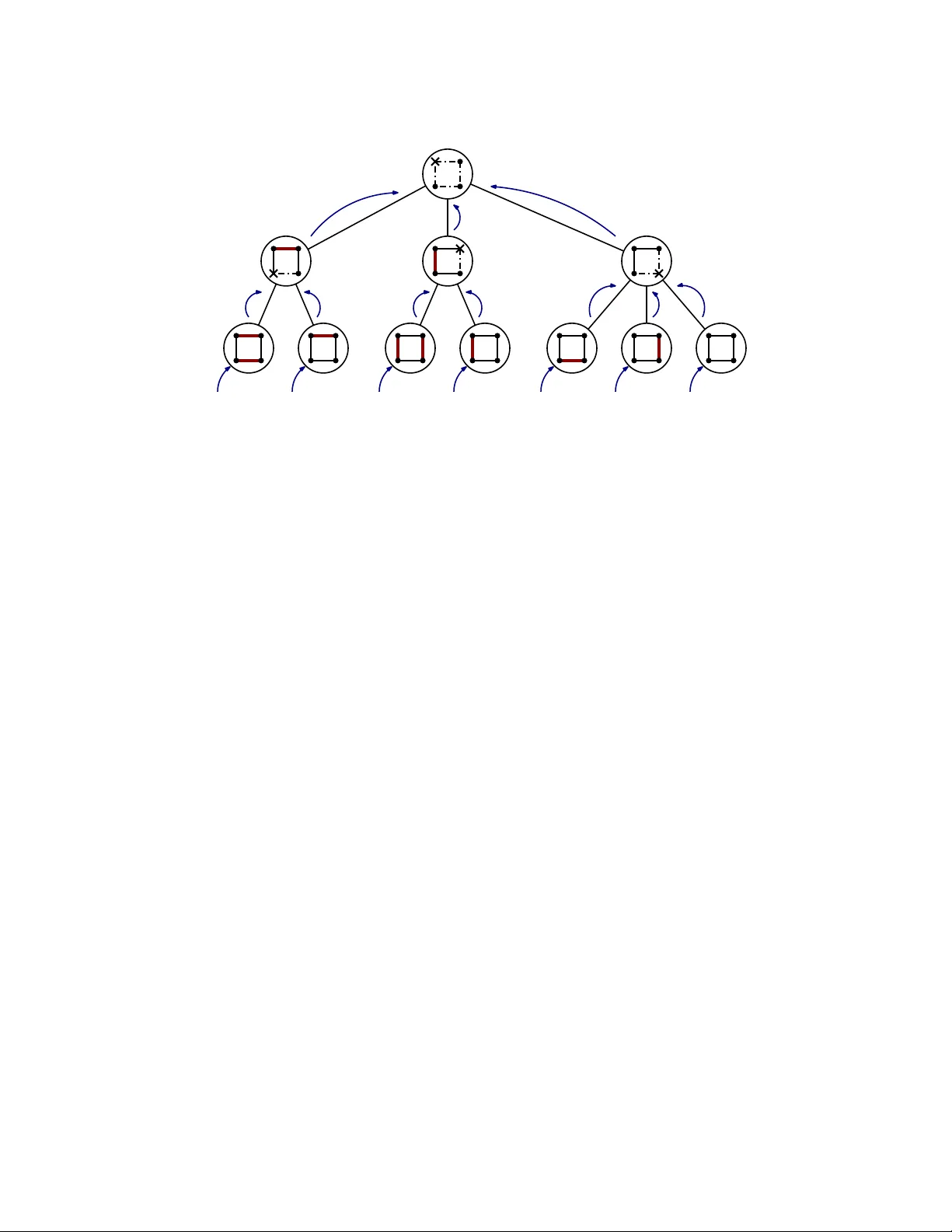
Constan t dela y Gra y co de en umeration of ideals and an tic hains in p osets Soﬁa Brenner ∗ and Ji ˇ r ´ ı Fink † Abstract W e presen t an algorithm that enumerates all ideals of an input p oset with constan t delay in Gra y co de order, i.e., such that consecutiv ely visited ideals diﬀer in at most three elemen ts. This answers a long-standing op en problem p osed by Pruesse and Ruskey , and improv es up on previous algorithms b y Pruesse and Rusk ey , Squire, Habib, Medina, Nourine and Steiner, as well as Abdo. Using the same tec hniques, we also obtain an algorithm that en umerates all an tichains of an input p oset with constant delay such that successiv ely visited an tichains diﬀer in at most three elements. As a key technical ingredient, we introduce a new p oten tial-based analysis framework for recursiv e algorithms, whic h we call the Pyr amid metho d . W e show that this metho d subsumes the Push-out metho d of Uno. Beyond the present application, the Pyramid metho d is a general framew ork to analyze recursive algorithms and may thus b e of indep enden t in terest. 1 In tro duction 1.1 Com binatorial en umeration The aim of an enumer ation algorithm is to list all ob jects in a (ﬁnite) set X exactly once. The set X is usually given by an implicit description and the task of the algorithm is to compute its elements. Clearly , the goal are algorithms that en umerate X eﬃcien tly while requiring small amoun ts of memory . Our fo cus lies on en umerating combinatorial ob jects, suc h as substructures of graphs, p osets, or subsets of permutations. The enumeration of combinatorial structures has a long history . The most basic algorithm to enumerate a set X identiﬁes X with the set of all strings of length n ov er an alphab et Σ. It non-deterministically c ho oses a letter of Σ for all n p ositions and accepts the resulting string if it b elongs to X . An early pap er b y Flo yd [ Flo67 ] conv erts this idea into a deterministic backtrac king ∗ Departmen t of Mathematics and Natural Sciences, Universit y of Kassel, Germany . Presen t address: Department of Applied Mathematics, Charles Univ ersity , Prague, Czec h Republic. E-mail address: sbrenner@mathematik.uni-kassel.de † Departmen t of Theoretical Computer Science and Mathematical Logic, Charles Univ ersity , Prague, Czech Re- public. E-mail address: fink@ktiml.mff.cuni.cz 1 algorithm, using pruning techniques and a strategy for choosing the righ t string to impro ve the p erformance. Read and T arjan [ R T75 ] enumerated graph substructures, suc h as spanning trees, cycles, and v arious kinds of paths. Their metho d was later referred to as the binary p artition metho d or Flashlight se ar ch (for instance, see [ MM24 ]). F ukuda and Matsui [ FM94 ] en umerated all p erfect matc hings in bipartite graphs in time O ( m | X | ) and space O ( nm ). Avis and F ukuda [ AF96 ] in tro duced the concept of r everse d se ar ch . They apply it to en umerate all triangulations of a set of n points in the plane, spanning trees of a graph, and topological orderings of an acyclic graph. Recen t w ork includes the pr oximity se ar ch framework by Conte, Grossi, Marino, Uno, and V ersari [ CU19 , CGM + 22 ], which they use to enumerate, for instance, maximal subgraphs or maximal trees in a giv en graph. Merino and M ¨ utze [ MM24 ] in tro duced a framew ork to list all vertices of 0 / 1-p olytop es via com binatorial optimization. This yields en umeration algorithms for n umerous combinatorial ob jects, including bases and indep enden t sets in a matroid, spanning trees, forests, matchings, or v ertex cov ers. Fink [ Fin25 ] derived a constant delay algorithm for listing p erfect matchings. F or man y enumeration algorithms, esp ecially in com binatorial enumeration, the size of the en umerated set X is exp onen tial in the input size. One thus rather measures the computation time sp en t b et ween t wo successiv ely visited elemen ts. An instruction is an elementary op eration executed in a constant time in a computation mo del, such as a deterministic random access machine or p oin ter mac hine. Let t ( i ) b e the num b er of instructions executed b efore the i -th elemen t is visited. The (worst-c ase) delay of an en umeration algorithm is the maximal time sp en t b et w een t wo successively visited elements, i.e., max i ∈{ 1 ,..., | X |− 1 } { t ( i + 1) − t ( i ) } . Clearly , the optimal outcome are algorithms with constant dela y . These algorithms are often called lo opless . As in many applications, the time b et w een t w o outputs diﬀers drastically , one often considers an av erage. The amortize d delay of an en umeration algorithm is the av erage computation time sp en t betw een tw o successiv e outputs, i.e., the total computation time of the algorithm divided by the num ber of its outputs. Note that some authors call this the aver age delay , and deﬁne the amortized delay of an algorithm as max i ∈{ 1 ,..., | X |} t ( i ) /i . In this paper, w e will also state bounds for this cardinalit y . In man y situations, one requires that successive outputs of an en umeration algorithm diﬀer only b y a small change, a so-called ﬂip . The deﬁnition of a ﬂip dep ends on the problem. A list- ing of the enumerated elements resp ecting this condition is called a c ombinatorial Gr ay c o de . A com binatorial generation problem on a set X can b e describ ed via its ﬂip gr aph . The v ertices of the ﬂip graph are the elemen ts of X , and t wo elements are connected whenev er they diﬀer by a ﬂip. Finding a com binatorial Gray co de th us amounts to ﬁnding a Hamiltonian path in the ﬂip graph. The classical binary r eﬂe cte d Gr ay c o de [ Gra53 ] lists all binary strings of a ﬁxed length n suc h that eac h tw o consecutive strings diﬀer in a single bit. The Steinhaus-Johnson-T r otter algo- rithm [ T ro62 , Joh63 , Ste64 ] lists p erm utations of length n suc h that t wo successively listed p erm u- tations diﬀer in a transp osition of adjacent v alues. In recent y ears, the area of com binatorial Gra y co des has seen a ﬂurry of results. A main line of researc h is the p ermutation language fr amework in- tro duced b y M¨ utze and collaborators (see [ HHMW20 ]). They pro ved the existence of combinatorial Gra y codes for n umerous classes of com binatorial ob jects, suc h as certain classes of pattern-a v oiding p erm utations [ HHMW20 ], quotien ts of the weak order [ HM21 ], rectangulations [ MM23a ], elimina- 2 tion trees [ CMM24 ], acyclic orientations [ CHMM23 ], binary trees [ GMN24 ], or graphs of regions of h yp erplane arrangemen ts [ BCM + 26 ]. In man y cases, the construction of the Gra y co des is explicit and can b e turned into an algorithm, but not in all cases a lo opless algorithm is kno wn. W e refer to M ¨ utze’s surv ey [ M¨ ut23 ] for a comprehensive o verview on combinatorial Gra y codes. 1.2 En umeration algorithms for p osets A p artial ly or der e d set (p oset) is a pair ( P , ⪯ ) consisting of a set P and a p artial or der ⪯ , that is, a reﬂexiv e, an tisymmetric, transitiv e relation, on P . In this pap er, w e only consider ﬁnite p osets. If the relation ⪯ is understo od from the context, w e simply write P for the p oset ( P , ⪯ ). F or u, v ∈ P with u ⪯ v and u  = v , w e write u ≺ v and sa y that u is smal ler than v , or that v is lar ger than u . The elemen ts u and v are inc omp ar able if neither u ⪯ v nor v ⪯ u holds. W e then call the set { u, v } an inc omp ar able p air . W e say that v c overs u , or that u and v are in a c over r elation , if u ≺ v and there is no z ∈ P with u ≺ z ≺ v . A useful to ol to represent a p oset is its Hasse diagr am . This is a graph dra wn in the plane whose vertices are the elemen ts of P . If v co vers u , we connect u and v b y an edge, and dra w v higher than u . See Figure 1 (a) for an illustration. The upset and downset of x ∈ P consist of all elements u ∈ P with x ⪯ u or u ⪯ x , resp ectiv ely . A subset I of P is an ide al if if it is downwar d-close d , i.e., for all u ∈ I , the downset of u is contained in I . The set of ideals of P will b e denoted by I ( P ). A chain in P is a subset consisting of pairwise comparable elemen ts of P , an antichain is a subset consisting of pairwise incomparable elements. An antic hain with precisely k elemen ts is called a k -antichain . P osets play a prominent role b oth in combinatorics and algorithms, and hence their algorith- mic aspects hav e been widely studied. F or instance, it was shown that v arious coun ting problems in p osets are #P-complete, such as coun ting the n umber of antic hains [ PB83 ] (and th us ideals, since ev ery p oset con tains the same n umber of ideals and an tichains), or linear extensions of a giv en p oset [ BW91 ]. Pruesse and Rusk ey [ PR94 ] derived an algorithm to en umerate linear exten- sions of an input p oset suc h that successiv ely enumerated extensions diﬀer b y one or t w o adjacen t transp ositions. This w as turned into a lo opless algorithm b y Canﬁeld and Williamson [ CW95 ]. In con trast, the lo opless enumeration of ideals has b een a long-standing open problem. W e refer to the discussions of this question in [ PR93 , PR94 , HMNS01 , M¨ ut23 , P ow25 ] for an o verview. The fastest enumeration algorithms for ideals in p osets, either listing in Gray co de order or in arbitrary order, hav e logarithmic dela y . F or k ∈ N , we sa y that a listing is a k -Gr ay c o de if t w o consecutiv ely visited ideals diﬀer in at most k elements (i.e, their symmetric diﬀerence has size at most k ). In the literature, the usual deﬁnition of a Gra y co de order is a 2-Gra y co de, i.e, successively listed ideals diﬀer in at most t wo elemen ts. In other w ords, one ideal arises from the other b y removing, adding, or exc hanging a single elemen t. In our algorithm, we deriv e a 3-Gray co de, i.e, successiv ely visited ideals may diﬀer in at most three elemen ts. Note that this does not c hange the asymptotic time complexity of the algorithms. Early algorithms [ La w79 , SB78 , PB83 ] list the ideals of a poset of size n with delay O  n 2  . Probably the ﬁrst algorithm with av erage delay O ( n ) was given b y Steiner [ Ste86 ]. Pruesse and Rusk ey [ PR93 ] obtain an algorithm for a (2-)Gray co de listing that runs in time O ( |I ( P ) | n ) 3 on general p osets, using a more general framew ork for an timatroids. Ho wev er, their algorithm lists every element twice. Medina and Nourine [ MN94 ] ga v e an algorithm with amortized dela y O ( d + ( P )), where d + ( P ) denotes the maximal out-degree in the Hasse diagram of P . Squire [ Squ95 ] (see also [ P ow25 ]) giv es an algorithm with a verage dela y O (log n ), how ev er not listing the ele- men ts in Gray co de order. Habib, Medina, Nourine and Steiner [ HMNS01 ] present a diﬀerent algorithm as part of their framework to enumerate distributive lattices, which lists the ideals with amortized delay O ( n ) in Gray co de order. F urther algorithms to en umerate ideals in Gray co de order with amortized delay O ( n ) w ere given b y Ab do [ Ab d09 , Ab d10 , Ab d13 ]. Merino and M ¨ utze [ MM23b , MM24 ] men tion that their m uc h more general framew ork to enumerate the v ertices of 0 / 1-polytop es yields an en umeration algorithm for p oset ideals as a special case. How ev er, this algorithm has delay O  n 4 log n  . F or antic hains, their framework also yields an algorithm, alb eit with delay O  n 2 . 5 log n  . Constan t av erage delay algorithms are kno wn for sp ecial p oset classes, suc h as forest p osets [ KR93 ] or interv al posets [ HNS97 ]. Man y of the ab o ve-men tioned algorithms, for instance those b y Squire and Ab do, rely on a recursiv e strategy that splits the ideals of the input p oset P into tw o subsets. One consists of the ideals which contain a ﬁxed element x ∈ P (and th us also its do wnset), and the other of the ideals not containing x (and thus none of the elements of its upset). The main diﬀerence lies in the c hoice of the element x . If the input p oset is a c hain, it is easy to see that this strategy yields at least logarithmic delay . In order to obtain a constant dela y algorithm, a diﬀerent recursiv e strategy is therefore needed. W e conclude this part by men tioning a v arian t of the ab o ve problem, the generation of ideals of a ﬁxed size in a p oset. Here, sucessiv ely visited ideals diﬀer in a swap of an element. This v arian t has attracted considerable atten tion ov er the years. In [ KR93 ], it was remark ed without pro of that their algorithm generating all ideals in forest posets can also b e used to generate ideals of a ﬁxed size. In [ PR93 ], this was then studied explicitly . Wild [ Wil14 ] ga ve an algorithm with O  n 3  dela y . This was recen tly impro ved b y Coumes, Bouadi, Nourine, and T ermier [ CBNT21 ], who used this to enumerate so-called skyline gr oups used in decision-making. They sho wed that these corresp ond to ideals of ﬁxed size in certain p osets. In this pap er, they gav e an algorithm that visits all ideals of size k in a p oset with delay O  ω 2  , where ω denotes the width of the input p oset. F or further applications of the en umeration of ideals of ﬁxed size, such as for co des and cov ering arrays, we refer to P o wers’ PhD thesis [ P ow25 ]. 1.3 Our results The aim of this pap er is to pro vide an algorithm for the enumeration of p oset ideals as w ell as an tichains with constant amortized dela y . This pap er has t w o parts: in the ﬁrst part, w e develop a metho d for p oten tial analysis, the Pyr amid c ondition , to analyze the amortized time complexit y of en umeration algorithms. In the second part, w e describ e an en umeration algorithm for ideals in a p oset in 3-Gray co de order. W e use the Pyramid condition to show that it has constant dela y . Using the same technique, w e also obtain a constan t delay algorithm for en umerating an tic hains. 4 1.3.1 Complexit y analysis and the Pyramid condition W e ﬁrst develop a new v arian t of the p oten tial analysis, which w e call the Pyr amid metho d . Our main in terest is to analyze com binatorial en umeration algorithms. Ho w ev er, the concept is not sp eciﬁcally tailored to this situation. The metho d exploits the idea that in a recursion tree of an en umeration algorithm, the leav es corresp ond to iterations generating output in quic k succession while requiring only small computation time whereas the opp osite occurs for the inner nodes. The idea of the amortization is th us to use the excess computation time of the leav es for the computations in nodes higher in the tree. T o this end, we use a p oten tial measuring the computation time that a child no de can spare for its parent. An illustration for a simple algorithm enumerating p erfect matc hings in an input graph is giv en in Figure 2 . F or an iteration X , let T ( X ) denote the n um b er of instructions needed for the execution of iteration X , C ( X ) denotes the set of iterations recursively called by X (i.e., the childr en of X ), and X ′ denotes the set of elements directly visited by X . W e refer to Section 2 for full deﬁnitions. The ab o ve idea is captured by the following deﬁnition: Deﬁnition 1.1 (Pyramid condition) . We say that a r e cursive algorithm A satisﬁes the Pyramid condition with r esp e ct to a p otential function Φ and time T ⋆ if ther e exists a c onstant µ > 0 such that for every iter ation X of A , it holds that X Y ∈ C ( X ) Φ( Y ) + µ | X ′ | − Φ( X ) ≥ T ( X ) T ⋆ . Let ∆ b e an upp er b ound for the num b er of instructions on a path from the ro ot to a leaf in the recursion tree. Our main result in this part is the follo wing: Theorem 1.2. L et A b e a r e cursive algorithm enumer ating a set X and assume that A satisﬁes the Pyr amid c ondition for a p otential function Φ and time T ⋆ . The total c omputation time to enumer ate X is O ( | X | T ⋆ − Φ( X )) , so the amortize d delay of A is O ( T ⋆ ) . The ﬁrst k elements of X ar e visite d in time O ( k T ⋆ + ∆) . In the time complexit y to en umerate the ﬁrst k elemen ts in Theorem 1.2 , the additiv e constant ∆ can b e view ed as a prepro cessing time needed at the b eginning, whereas each visited element requires T ⋆ additional time. W e no w turn from amortized dela y to w orst-case delay analysis. It is w ell-known that an algorithm with amortized delay T ⋆ can b e turned in to an algorithm with w orst-case delay T ⋆ , but at the p ossible price of exp onen tial memory consumption. Using an idea that w as originally presented b y Uno in an unpublished technical rep ort [ Uno03 ], we obtain the following de-amortization result for algorithms satisfying the Pyramid condition: Theorem 1.3 (W orst-case delay) . L et A b e a r e cursive algorithm enumer ating a set X that satisﬁes the Pyr amid c ondition with r esp e ct to a p otential Φ and time T ⋆ . Assume that the change b etwe en two suc c essively visite d elements of A c an b e stor e d using O (1) memory and that these changes c an 5 b e applie d in time O ( T ⋆ ) . Then ther e exists an A lgorithm ˆ A which enumer ates X in the same or der as A with worst-c ase delay O ( T ⋆ ) , while r e quiring O (∆ /T ⋆ ) additional sp ac e and O (∆) additional time for the initialization. Whereas there is no general upp er b ound for ∆, in man y applications, the depth of the recursion tree as w ell as the num b er of instructions along a longest path from a root to the leaf is polynomially b ounded in the input size. In this case, b oth the additional space requirement as well as the initialization time for the algorithm A ′ from Theorem 1.3 are p olynomial in the input size. As a t ypical example, consider an easy enumeration algorithm, for instance for spanning trees, that in eac h iteration c ho oses an ob ject of the input graph, such as an edge to b e included or excluded. Clearly , both the depth of this recursion tree and the num b er of iterations on a path from the ro ot to a leaf are at most linear in the input size. Comparison with the Push-out metho d Uno [ Uno15 ] devised a metho d to analyze the amor- tized time complexity of recursiv e algorithms, the so-called Push-out metho d . He employs it to show that v arious com binatorial enumeration algorithms, for instance, for enumerating elimination or- derings, matchings forests, connected induced subgraphs, or spanning trees in a given graph, hav e constan t amortized dela y . W e prov e that the Pyramid method subsumes the Push-out metho d: Theorem 1.4. If a r e cursive enumer ation algorithm A satisﬁes Uno’s Push-out c ondition with time T ⋆ (i.e., the metho d yields an amortize d time c omplexity T ⋆ ), then ther e exists a p otential function Φ such that A satisﬁes the Pyr amid c ondition with r esp e ct to Φ and time T ⋆ . Theorem 1.4 states that ev ery algorithm that has amortized dela y T ⋆ b y the Push-out method can b e analyzed by the Pyramid method, yielding the same bound T ⋆ for the amortized dela y . A t the same time, our algorithms for en umerating ideals and antic hains in p osets are examples of algorithms for which the Push-out metho d cannot b e used to pro v e constan t amortized dela y , whic h in turn can b e prov ed using the Pyramid metho d. W e give an example p oset in Example 3.13 . This shows that the Pyramid metho d is strictly more p ow erful than the Push-out metho d. The intuition is that in the Push-out metho d, every child Y sends O ( T ( Y )) to its parent. In con trast, the Pyramid metho d is a more v ersatile framew ork as it allows to transfere arbitrary amoun ts of computation time b et ween children and parent iterations. More precisely , it follows that the Push-out condition is satisﬁed if and only if Pyramid condition holds for a p oten tial of the form Φ( X ) = O ( T ( X )). In this case, b oth metho ds can b e applied to pro ve constant amortized dela y . 1.3.2 Constan t delay en umeration of p oset ideals The main result of this pap er is a recursive en umeration algorithm for ideals in a p oset that has constan t delay and lists the ideals such that consecutiv ely visited ideals diﬀer in at most three elemen ts. W e ﬁrst describ e a v ersion that lists th e ideals in arbitrary order with constan t amortized dela y . A description in pseudoco de is given in Algorithm 1.1 . Subsequently , w e demonstrate how 6 to reﬁne this algorithm as to visit the ideals in Gra y co de order and in vok e Theorem 1.3 to pass to constan t dela y . Algorithm 1.1: Enumeration of all ideals in a p oset (basic version). 1 Pro cedure Enumerate( Poset P , arr ay I of elements outside P ) 2 if P = ∅ then 3 Visit( I ) 4 else 5 Find a longest chain C in P 6 Construct auxiliary sets L 2 , . . . , L k and S 0 , . . . , S k − 1 7 P ′ ← S 0 // P ′ = P 0 8 Enumerate( P ′ , I ) // Enumerate ideals in P 0 9 for i ← 1 , . . . , k do 10 P ′ ← ( P ′ \ L i ) ∪ S i // P ′ = P i 11 I ← I ∪ L i ∪ { c i } 12 Enumerate( P ′ , I ) // Enumerate ideals in P i 13 I ← I \ P // Remove all elements added to I by this iteration. 14 Pro cedure Main( Poset P ) 15 Relab el P suc h that u ⪯ v implies u ≤ v 16 Enumerate ( P , ∅ ) Recursiv e structure One main diﬀerence of our algorithm compared to the existing ones is the recursiv e structure. In contrast to the previous algorithms, which split the set of ideals into tw o parts, dep ending on whether or not they contain a ﬁxed elemen t x ∈ P , we partition the ideals using a longest c hain. This enables us to obtain constan t dela y if the input poset is a chain, whic h is not possible with the previously emplo yed recursive techniques (see, for instance, [ Squ95 , Ab d13 ]). Let C b e a longest c hain of P and write C = { c 1 , . . . , c k } with c 1 ⪯ · · · ⪯ c k . The recursion of Algorithm 1.1 uses a partition of the ideals of P in to k + 1 sets I 0 ( P ) , . . . , I k ( P ), dep ending on the largest elemen t of C contained in the ideal (or the fact that none exists). F ormally , for i > 0, the set I i ( P ) consists of the ideals I of P suc h that c i is the maximal element in I ∩ C . The set I 0 ( P ) con tains those ideals of P that do not con tain an elemen t of C . W e no w deﬁne the subposets P 0 , . . . , P k of P on which we call the recursion. F or i = 0 , . . . , k , the p oset P i is the subp oset of P consisting of all elemen ts u ∈ P with u ⪯ c i and u ⪰ c i +1 (using the conv en tion that c 0 ⪯ u ⪯ c | C | +1 for all u ∈ P ). The crucial insigh t used for the recursion is that there is a bijection b et ween the ideals in I i ( P ) and the ideals of P i (see Lemma 3.3 ). It maps an ideal I ∈ I i ( P ) to I \ D i , where D i denotes the downset of c i . T o obtain the ideals in I i ( P ), w e th us recursiv ely compute the ideals in P i and add the set D i to each. Figure 1 illustrates the deﬁnition of P i and the partition of the ideals into the sets I i ( P ). 7 c 1 c 2 c 3 c 4 a b e d e c 1 c 2 c 3 c 4 a b e d D 0 = ∅ D 0 ∪ ∅ = ∅ D 0 ∪ { d } = { d } D 1 = { c 1 } D 1 ∪ ∅ = { c 1 } D 1 ∪ { a } = { c 1 , a } D 1 ∪ { d } = { c 1 , d } D 1 ∪ { a, d } = { c 1 , a, d } D 1 ∪ { a, b, d } = { c 1 , a, b, d } c 2 c 3 c 4 a b d e D 2 = { c 1 , c 2 , d } D 2 ∪ ∅ = { c 1 , c 2 , d } D 2 ∪ { a } = { c 1 , c 2 , d, a } D 2 ∪ { e } = { c 1 , c 2 , d, e } D 2 ∪ { a, e } = { c 1 , c 2 , d, a, e } D 2 ∪ { a, b, e } = { c 1 , c 2 , d, a, b, e } D 1 ∪ { a, b } = { c 1 , a, b } D 2 ∪ { a, b } = { c 1 , c 2 , d, a, b } c 1 c 2 c 3 c 4 a b e d D 3 = { c 1 , c 2 , c 3 , a, d } D 3 ∪ { b } = { c 1 , c 2 , c 3 , a, d, b } D 3 ∪ { e } = { c 1 , c 2 , c 3 , a, d, e } D 4 = { c 1 , c 2 , c 3 , c 4 , a, d, e } D 4 ∪ ∅ = { c 1 , c 2 , c 3 , c 4 , a, d, e } D 4 ∪ { b } = P c 1 c 2 c 3 c 4 b e d D 3 ∪ ∅ = { c 1 , c 2 , c 3 , a, d } D 3 ∪ { b, e } = { c 1 , c 2 , c 3 , a, d, b, e } c 1 c 1 c 2 c 3 c 4 a b e d P 0 = { d } P 1 = { a, b, d } P 2 = { a, b, e } P 3 = { b, e } P 4 = { b } S 0 = { d } S 1 = { a, b } S 2 = { e } S 3 = ∅ S 4 = ∅ L 1 = ∅ L 2 = { d } L 3 = { a } L 4 = { e } L 5 = { b } ( a ) ( b ) Figure 1: (a) Example of a poset P , together with the subp osets P 0 , . . . , P 4 as well as the sets S 0 , . . . , S 4 and L 1 , . . . , L 5 , visualized by its Hasse diagram. (b) The sets D i and the ideals in I i ( P ) for i = 0 , . . . , 4. Every ideal in I i ( P ) is of the form I ′ ∪ D i , where I ′ is an ideal of P i . The elements in P i and D i are marked in blue and black, resp ectiv ely . 8 T o eﬃcien tly up date the currently pro cessed p oset when transitioning from P i to P i +1 and compute the downset D i of c i , w e use auxiliary subsets S 0 , . . . , S k and L 1 , . . . , L k +1 deﬁned b e- lo w. These are computed sim ultaneously with the c hain C . W e will no w giv e details on these computations and their time complexity . Computing c hains and updates F or computing a longest chain, we derive a sp ecial algorithm using an an tic hain decomp osition in time O ( n + q ), where q is the n umber of incomparable pairs, as the time complexity O  n 2  of the classical top ological sorting algorithm is not suﬃcient for this task. Then, we compute sets S 0 , . . . , S k and L 1 , . . . , L k +1 in time O ( n + q ). Here S i consists of all elemen ts u ∈ P \ C with u ≻ c i and u ≻ c i +1 (in other w ords, c i is the largest elemen t on C that is smaller than u ). Symmetrically , w e deﬁne L i as the set of elements u ∈ P \ C with u ≺ c i and u ≺ c i − 1 . As C is a longest chain, we hav e S k = L 1 = ∅ . Note that with this notation, we hav e D i = D i − 1 ∪ L i ∪ { c i } and P i = ( P i − 1 \ L i ) ∪ S i . W e use these rules to up date the curren t p oset P ′ on whic h the recursion is called, and the current set I of elemen ts that w ere already added to the ideal under construction. Let n i = | P i | for i = 0 , . . . , k . When processing the p osets in the ordering P 0 , . . . , P k , we can show that ev ery element of P i is added and deleted a constant n umber of times, so for the up dating, w e require a total n umber of changes that is in O ( P n i ) ≤ O ( n + q ). The key observ ation used for the complexity analysis of the construction of C is that there is at most one comparison for every incomparable pair and every elemen t is compared to at most one smaller elemen t. A similar strategy is applied for computing all sets S i , L i , D i and P i . In order to analyze the complexit y of whole algorithm, we apply the Pyramid metho d with a potential function of the form Φ( P ) = α + β n + γ q + δ t with α, β , γ , δ ∈ N . Here, t denotes the num b er of incomparable triples (i.e., 3-antic hains) in P . Gra y co de listings The basic v ersion of Algorithm 1.1 lists the ideals in arbitrary order. W e presen t a reﬁned version that lists the ideals of the input p oset P suc h that ev ery pair of consecu- tiv ely visited ideals diﬀers in at most three elemen ts. This is ac hiev ed b y c ho osing a special ordering as well as prescrib ed start and end ideals for each of the recursive calls on P 0 , . . . , P k . Using the tec hnique from Theorem 1.3 , w e can con vert this into a lo opless algorithm. By a result of Pruesse and Ruskey [ PR93 ], the ﬂip graph on ideals of P with ﬂips b et w een ideals diﬀering in at most tw o elements has a Hamiltonian path. It is, how ever, not known whether suc h a path can b e computed with constan t amortized dela y . W e b eliev e that it migh t b e p ossible to reﬁne our algorithm suc h that consecutively visited ideals diﬀer in at most tw o elements, while preserving constant dela y . Note, how ever, that this do es not inﬂuence the asymptotic runtime of the algorithm. W e summarize our results for en umerating p oset ideals: Theorem 1.5. A lgorithm 1.1 enumer ates al l ide als of a p oset P on n elements with c onstant amortize d delay while r e quiring O  n 2  sp ac e and O  n 2  time for the initialization. F or k ∈ N , 9 the ﬁrst k ide als ar e visite d in time O ( k + n ( n + q )) , wher e q ∈ O  n 2  denotes the numb er of 2 -antichains in P . We c an r eﬁne Algorithm 1.1 to a lo opless algorithm that visits the ide als of P in Gr ay c o de or der, i.e, such that two c onse cutively visite d ide als diﬀer in at most thr e e elements. 1.3.3 Constan t delay algorithms for enumerating an tichains Using the same tec hniques as for ideals, w e obtain a constant delay en umeration algorithm for an tichains (Algorithm 1.2 ). As ab o v e, we can reﬁne the algorithm to list the antic hains in Gray co de order, i.e, suc h that successiv ely visited antic hains diﬀer in at most three elemen ts. Algorithm 1.2: Enumeration of all an tichains in a poset (basic version). 1 Pro cedure Enumerate( Poset P , arr ay of elements A outside P ) 2 if P is empty then 3 Visit( A ) 4 else 5 Find a longest chain C in P 6 Construct L 2 , . . . , L k and S 0 , . . . , S k − 1 7 P ′ ← S 0 // P ′ = P 1 8 Enumerate( P ′ , A ∪ { c 1 } ) 9 for i ← 2 , . . . , k do 10 P ′ ← ( P ′ \ L i ) ∪ S i − 1 // P ′ = P i 11 Enumerate( P ′ , A ∪ { c i } ) 12 Enumerate( P \ C , A ) 13 Pro cedure Main( Poset P ) 14 Sort the elemen ts so that u ⪯ v implies u ≤ v 15 Enumerate ( P , ∅ ) Theorem 1.6. Algorithm 1.2 enumer ates al l antichains of a p oset P on n elements with c onstant amortize d delay, and r e quir es O  n 2  sp ac e and O  n 2  time for the initialization, wher e q ∈ O  n 2  denotes the numb er of 2 -antichains in P . The ﬁrst k antichains ar e visite d in time O ( k + n ( n + q )) . We c an r eﬁne A lgorithm 1.2 to a lo opless algorithm that visits the antichains of P in Gr ay c o de or der, i.e, such that two c onse cutively visite d antichains diﬀer in at most thr e e elements. This paper is organized as follows: in Section 2 , we describ e the Pyramid condition, a new metho d for the p otential analysis of recursive algorithms. In Section 3 , we describe an algorithm that enumerates ideals in a p oset with constan t delay . In Section 4 , we giv e a constant dela y algorithm for an tic hains. 10 R X 1 X 2 Y 11 Y 12 Y 21 Y 22 Y 31 Y 32 Y 33 X 3 Φ( X 3 ) Φ( X 2 ) Φ( X 1 ) Φ( Y 12 ) Φ( Y 11 ) Φ( Y 22 ) Φ( Y 31 ) Φ( Y 33 ) Φ( Y 21 ) µ µ µ µ µ µ µ Figure 2: Recursion tree for enumerating all matchings in a graph G (see Example 2.1 ). In each iteration (no de of the tree), a v ertex v of G (mark ed with × ) is selected. The recursiv e calls corresp ond to selecting an edge inciden t to v to b e included in the matching (marked in red) or deciding to include none of the edges incident to v (excluded edges are mark ed in solid black). A t the b eginning, the status of all edges in G is undetermined (dashed). Ev ery leaf of the recursion tree corresp onds to a matching of G . 2 P oten tial analysis for combinatorial en umeration In this section, w e describ e a new method for p oten tial analysis, called Pyr amid metho d . It will b e used to sho w that the algorithms for enumerating ideals and antic hains in posets (Algorithms 1.1 and 1.2 ) hav e constant amortized delay . W e stress, ho wev er, that the presented metho ds can b e applied to an y enumeration algorithm, and migh t th us b e of indep enden t interest. In Section 2.1 , w e introduce the setup of the analyzed algorithms. In Section 2.2 , w e describ e the Pyramid method. In Section 2.3 , w e discuss ho w turn an algorithm that satisﬁes the Pyramid condition with amortized dela y T ∗ in to an algorithm with worst-case dela y T ∗ , provided that the elemen ts are visited in Gra y code order. 2.1 Recursiv e algorithms W e now describe the setup of the recursive algorithms that w e analyze using terminology similar to Uno [ Uno15 ]. Let S b e a set to b e en umerated using a recursive algorithm A . As an example, consider the follo wing example en umerating all matc hings of a graph. Example 2.1. We c onsider a simple algorithm to enumer ate al l matchings in an input gr aph G (also se e [ Uno15 , Se ction 5]). F or an il lustr ation, se e Figur e 2 . The algorithm maintains a set of e dges include d in the matching. A t the b e ginning, this set is empty. In e ach iter ation, we ﬁx a vertex v of G and let e 1 , . . . , e k b e the e dges incident to v . Cle arly, every matching of G c ontains at most one of these e dges. Thus, for e ach i ∈ { 1 , . . . , k } , ther e is a r e cursive c al l of the function 11 that includes the e dge e i in the matching, to gether with one additional c al l r epr esenting the c ase that none of the e dges e 1 , . . . , e k is include d. Let T ( A ) b e a recursion tree representing the recursion calls in A . Every no de of T ( A ) corre- sp onds to a recursiv e function call of A and p oten tially some additional non-recursiv e computation. An iter ation of the recursiv e function A is its execution, excluding the computation in the func- tion recursively called by the iteration. W e can identify the iterations of A with the no des of its recursion tree, and use them interc hangeably . Asso ciated to eac h iteration is a subset X ⊆ S that con tains the elements that are visited in this iteration or one of its recursiv e calls. W e use the set X to lab el and identify the iteration. In iteration X , a partition X = X 1 ˙ ∪ · · · ˙ ∪ X k ˙ ∪ X ′ is derived, where X 1 , . . . , X k  = ∅ . Here, X ′ denotes the set of elements directly visited by the iteration X , and may b e empty . The function is recursively called for the sets X 1 , . . . , X k . These iterations are called the childr en of X as in the recursion tree, the no des corresp onding to X 1 , . . . , X k are the c hildren of the no de corresp onding to X . The set of c hildren of X is denoted b y C ( X ), and w e call X the p ar ent of X 1 , . . . , X k . The r o ot iter ation is the iteration without parent, and a le af iter ation is an iteration without any c hildren. A subtr e e of an iteration X contains X and all its descendan ts, i.e., iterated children sets. In our applications, w e usually encounter the special case that if | X | ≥ 2, no element is directly visited by the iteration X and all elemen ts of X are passed on to the recursiv e calls, and if | X | = 1, the unique elemen t of X is visited and no recursion is called. That is, we hav e X ′ = ∅ if | X | > 1 and X ′ = X if | X | = 1. As customary in sublinear en umeration, w e assume that every visited element is pro vided by a pointer to a data structure (usually an array) and this data structure is modiﬁed during the en umeration before another element is visited. 2.2 P oten tial analysis and the Pyramid condition In this section, we describe a p oten tial analysis metho d which w e call Pyr amid metho d . The p otential analysis is a well-established technique to analyze the amortized time complexit y of data structures (for instance, see [ CLRS09 ]). W e no w deﬁne a v arian t to analyze the amortized complexit y of recursiv e algorithms, in particular for com binatorial enumeration. The in tuition is that for many en umeration algorithms, most elements of the enumerated set are visited in leaf iterations. At the same time, these iterations tend to require only small computation time. In other w ords, the leaf iterations usually visit elements in quick succession while requiring little computation time, whereas the inner no des of the tree visit less elements and require more computation time. Leaf iterations thus tend to ha ve a p ositiv e balance b et w een used computation time and generated output, whereas inner no des hav e a negativ e one. F or the amortized time analysis, this suggests a mo del in whic h c hildren no des pass excess time resources to their paren t. This approac h was, for instance, tak en by Uno’s Push-out method [ Uno15 ], whic h allow ed to show that v arious en umeration algorithms hav e constant dela y . In our mo del, we use c oins as ﬁxed time units. Each coin pays for T ⋆ instructions, where T ⋆ can b e any ﬁxed function of the input size. Ultimately , T ⋆ will b e the amortized dela y that our 12 analysis yields. In our applications, we usually show that our algorithm has constan t dela y , which corresp onds to setting T ⋆ = O (1). If an iteration visits an element, it is rewarded by obtaining a ﬁxed constan t n umber µ > 0 of coins. When executing instructions, the corresponding amount of coins needs to b e pay ed by the algorithm. F ollo wing the ab ov e intuition, our mo del mak es c hildren iterations pass coins to their paren ts. This is mo deled by a p oten tial function Φ. It assigns eac h iteration X , i.e., each no de of the recursion tree, a potential Φ( X ) > 0 representing the num b er of coins that X passes to its paren t. An iteration X thus obtains µ coins for ev ery visited element of X ′ as w ell as P Y ∈ C ( X ) Φ( Y ) coins from its c hildren, and passes Φ( X ) coins to its parent (see Figure 2 for an illustration for the algorithm from Example 2.1 ). In tuitively , this mechanism is sustainable if Φ and T ⋆ are chosen in a w a y that every node can pa y its own computation time. That is, the diﬀerence b et ween the µ | X ′ | + P Y ∈ C ( X ) Φ( Y ) coins that an iteration X obtains and the Φ( X ) coins it sends to its parent m ust b e suﬃcient to pa y for the execution of the instructions in X , i.e, at least T ( X ) /T ⋆ coins are needed. This is captured by the following condition: Deﬁnition 2.2 (Pyramid condition) . A r e cursive algorithm A satisﬁes the Pyramid condition with r esp e ct to a p otential function Φ and time T ⋆ if for every iter ation X of A , it holds that X Y ∈ C ( X ) Φ( Y ) + µ | X ′ | − Φ( X ) ≥ T ( X ) T ⋆ . Note that this requires the ro ot iteration R to pro vide Φ( R ) coins to pass to its (non-existing) paren t. This additional time resource could be used to cov er instructions executed outside the recursion, such as reading the input or initialization. W e no w sho w that this condition can indeed b e used to obtain b ounds for the amortized dela y of a recursiv e algorithm. 2.2.1 Amortized dela y Lemma 2.3. L et A b e a r e cursive algorithm enumer ating a set X that satisﬁes the Pyr amid c on- dition for some p otential function Φ and time T ⋆ . L et X b e an iter ation of A . Then the numb er of instructions exe cute d in a subtr e e of X is at most T ⋆ ( µ | X | − Φ( X )) . Pr o of. W e pro ve the lemma b y the induction on the size of X . The num ber of instructions executed in the subtree of X is at most T ( X ) + X Y ∈ C ( X ) T ⋆ ( µ | Y | − Φ( Y )) = T ⋆   T ( X ) T ⋆ + Φ( X ) − µ | X ′ | − X Y ∈ C ( X ) Φ( Y )   + T ⋆ ( µ | X | − Φ( X )) ≤ T ⋆ ( µ | X | − Φ( X )) . 13 Y 1 Y 2 Y 3 L j L i L Figure 3: Illustration of the pro of of Lemma 2.5 . Note that this inequality holds b oth when X is a leaf, i.e, C ( X ) = ∅ , as well as when C ( X ) is non-empt y . In the second step, we used that | X | = | X ′ | + P Y ∈ C ( X ) | Y | . The last inequality follows from the Pyramid condition. This immediately yields the following: Theorem 2.4. L et A b e a r e cursive algorithm enumer ating a set X and assume that A satisﬁes the Pyr amid c ondition for some p otential function Φ and time T ⋆ . The total time to enumer ate X is O ( | X | T ⋆ − Φ( X )) . Thus A has amortize d delay O ( T ⋆ ) . W e stress that this only takes the computations executed within the recursion in to accoun t, in particular not reading the input and p ossible initialization. 2.2.2 Visiting times An en umeration algorithm deﬁnes an ordering on the enumerated set X , namely the ordering in whic h it visits the elements of X . W e no w analyze the num b er of instructions that are executed b et w een visiting the i -th and the j -th elemen t of this ordering. Let ∆ be an upp er bound for the n umber of instructions executed by all iterations on a path in the recursion tree from the ro ot to a leaf iteration. Lemma 2.5. L et A b e a r e cursive algorithm enumer ating a set X and assume that A satisﬁes the Pyr amid c ondition with time T ⋆ . F or every 1 ≤ i ≤ j ≤ | X | , the numb er of instructions δ ij exe cute d b etwe en visiting the i -th element and the j -th element of X is at most 2∆ + ( j − i ) µT ⋆ − 1 . F urthermor e, the numb er of instructions exe cute d b efor e visiting the j -th element is at most ∆ + j µT ⋆ − 1 . Pr o of. F or an illustration, see Figure 3 . Let L i and L j b e the iterations in whic h the i -th and the j -th element are visited, resp ectiv ely . Let L b e the lo west common ancestor of L i and L j in the recursion tree. Let Y 1 , . . . , Y k denote those iterations executed b etw een L i and L j whose paren ts are on the paths from L to L i and L j , but that are not contained in the paths themselv es. 14 Then δ ij is b ounded from ab o v e b y the n umber of instructions on the paths, together with the instructions in the subtrees of Y 1 , . . . , Y k . The num ber of instructions on the paths is at most 2∆ − T ( L ) ≤ 2∆ − 1. By Lemma 2.3 , the n umber of instructions executed in the subtree of iteration Y i is at most µT ⋆ | Y i | . Note that the sets Y 1 , . . . , Y k con tain all elements visited b et ween i and j and that each elemen t is con tained in precisely one set Y i . Th us P k i =1 µT ⋆ | Y i | = µT ⋆ ( j − i ). This yields δ ij ≤ 2∆ + µT ⋆ ( j − i ) − 1. The pro of of the second part follo ws analogously by summing the instructions executed along a path from the ro ot to L j as w ell as in all subtrees whose ro ot has a parent on this path and whic h are executed before L j (note that the j -th element is not con tained in an y of these subtrees). This immediately yields the following result: Theorem 2.6. L et A b e a r e cursive algorithm enumer ating a set X and assume that A satisﬁes the Pyr amid c ondition with time T ⋆ . Then A enumer ates the ﬁrst k elements in time O ( k T ⋆ + ∆) . Note that this yields an upp er b ound on the amortized delay deﬁned in the sense of Capp elli and Strozecki [ CS23 ]. 2.2.3 Comparison with Uno’s Push-out metho d Uno [ Uno15 ] presen ted a method called Push-out to analyze the amortized complexity of recursive en umeration algorithms. It uses the follo wing condition: Deﬁnition 2.7 (Push-out condition [ Uno15 ]) . A r e cursive algorithm satisﬁes the Push-out con- dition with time T ⋆ if ther e exist c onstants α > 1 and β ≥ 0 such that for al l iter ations X , we have X Y ∈ C ( X ) T ( Y ) ≥ αT ( X ) − β ( | C ( X ) | + 1) T ⋆ . Theorem 2.8 ([ Uno15 , Theorem 1]) . A r e cursive enumer ation algorithm that satisﬁes the Push-out c ondition with time T ⋆ has amortize d delay O ( T ⋆ ) . W e prov e that the Pyramid metho d subsumes the Push-out metho d b y deﬁning a particular p oten tial function for which b oth metho ds giv e equiv alent conditions. Prop osition 2.9. If a r e cursive algorithm A satisﬁes the Push-out c ondition with time T ⋆ for c onstants α > 1 and β ≥ 0 , the A satisﬁes the Pyr amid c ondition with time T ⋆ for the p otential function Φ( X ) = T ( X ) ( α − 1) T ⋆ + 3 β α − 1 . 15 Pr o of. W e hav e X Y ∈ C ( X ) Φ( Y ) − Φ( X ) = 1 ( α − 1) T ⋆   X Y ∈ C ( X ) T ( Y ) − T ( X )   + 3 β α − 1 ( | C ( X ) | − 1) ≥ 1 ( α − 1) T ⋆ (( α − 1) T ( X ) − β ( | C ( X ) | + 1) T ⋆ ) + β α − 1 (3 | C ( X ) | − 3) = T ( X ) T ⋆ + β α − 1 (2 | C ( X ) | − 4) ≥ T ( X ) T ⋆ . The ﬁrst inequalit y uses the Push-out condition and the second one follo ws from the fact that ev ery inner no de of the recursion tree has at least tw o children. This result, combined with Theorem 2.4 , yields an alternativ e proof of [ Uno15 , Theorem 1]. Moreo ver, it shows that any enumeration problem analyzed by the Push-out metho d can also b e analyzed b y the Pyramid method, yielding the same amortized time complexity . In particular, w e can inv ok e Lemma 2.5 to determine the complexity of enumeratin g the ﬁrst k elements. This applies, for instance, to the enumeration of elimination orderings, matc hings forests, connected induced subgraphs, and spanning trees in a giv en graph studied in [ Uno15 ]. In Example 3.13 b elo w, we sho w that for Algorithm 1.1 en umerating ideals in a p oset, the Push-out method fails to sho w that the giv en algorithm has constan t dela y , whereas w e can sho w this with the Pyramid metho d. The same applies for Algorithm 1.2 . 2.3 W orst-case delay for Gray co de algorithms W e now describe a method to deamortize a recursive algorithm A that satisﬁes the Pyramid con- dition with time T ⋆ , i.e., A has amortized delay T ⋆ , pro vided that A en umerates the elemen ts in so-called Gr ay c o de or der . The goal is to obtain an algorithm ˆ A with worst-case delay O ( T ⋆ ) that enumerates the elements in the same ordering as A . This metho d was already describ ed in an unpublished tec hnical rep ort by Uno [ Uno03 ]. W e include a description here for completeness. Cap elli and Strozecki [ CS23 ] present a diﬀeren t approach for deamortization. W e assume that A en umerates all elements in a Gr ay c o de or der . This means that the mo di- ﬁcations in the data structures b et ween t wo consecutiv ely visited elements can b e stored in O (1) memory , and the data structure can b e modiﬁed for the next element in the w orst-case time O ( T ⋆ ). The deamortization of A uses an auxiliary queue Q with 2∆ µT ⋆ slots. Ev ery slot stores the c hanges b et ween tw o consecutively visited elements. Algorithm ˆ A sim ulates the computation of Algorithm A as follows: whenever A visits an element, Algorithm ˆ A stores it in the queue Q . More precisely , ˆ A sav es the changes in the data structure b et ween tw o elements consecutively visited b y A , thereb y using one slot of Q . 16 In the beginning, ∆ instructions of A are executed. Subsequen tly , after eac h µT ⋆ instructions of Algorithm A , Algorithm ˆ A visits and remov es the ﬁrst elemen t in Q . Concretely , ˆ A applies all c hanges stored in the ﬁrst slot of Q to the data structure. By assumption, this can b e computed in time O ( T ⋆ ). F urthermore, whenev er Q con tains more than 2∆ µT ⋆ elemen ts, Algorithm ˆ A visits and remo ves the ﬁrst elemen t in Q . It remains to pro ve the following: Lemma 2.10. The queue Q is non-empty whenever Algorithm ˆ A ne e ds to visit an element. Pr o of. Assume that Q is empt y when Algorithm ˆ A needs to visit the j -th elemen t. First assume that Q has never b een full b efore. When ˆ A needs to visit the j -th element, Algorithm A has executed j µT ⋆ + ∆ instructions. By Lemma 2.5 , Algorithm A executed at most j µT ⋆ + ∆ − 1 instructions b efore visiting the j -th element. This contradicts the assumption that Q is empt y . No w assume that the last o ccasion when Q was full was when A visited the i -th element. F rom the size of the queue, it follo ws that A executed ( j − i ) µT ⋆ + 2∆ instructions. How ev er, by Lemma 2.5 , Algorithm A executed at most ( j − i ) µT ⋆ + 2∆ − 1 instructions betw een visiting the i -th and the j -th element. This is a con tradiction. This yields the following theorem for deamortization: Theorem 2.11. L et A b e a r e cursive algorithm satisfying the Pyr amid c ondition with time T ⋆ . F urthermor e, assume that the change b etwe en two suc c essively visite d elements of A c an b e stor e d using O (1) memory and that these changes c an b e applie d in time O ( T ⋆ ) . Then A lgorithm ˆ A enu- mer ates al l elements in the same or der as A with worst-c ase delay O ( T ⋆ ) while r e quiring O (∆ /T ⋆ ) additional sp ac e and O (∆) additional time for the initialization. 3 Constan t amortized time en umeration of p oset ideals In this section, w e present a recursive algorithm (Algorithm 1.1 ) that enumerates all ideals of an input p oset ( P , ⪯ ) with constant amortized delay . 3.1 Preliminaries W e ﬁrst in tro duce some auxiliary structures that will b e used to deﬁne the recursiv e structure of our algorithm. Throughout, let P b e a p oset and ﬁx a longest c hain C of P . Let k = | C | . The recursion of the enumeration algorithm uses a partition of the ideals of P in to k + 1 groups, dep ending on the maximal elemen t of C con tained in the ideal or the fact that the ideal do es not con tain an y element of C , resp ectively . F or an illustration of the follo wing deﬁnitions, see Figure 1 . Let I ( P ) denote the set of ideals of P . W rite C = { c 1 , . . . , c k } with c 1 ≺ · · · ≺ c k . F or simplicity , we add t wo virtual elemen ts c 0 and c k +1 , whic h are smaller and larger than all elements in P , resp ectiv ely . F or I ∈ I ( P ), let ζ ( I ) = max { i : c i ∈ I } and set ζ ( I ) = 0 if I ∩ C = ∅ . F or i ∈ { 0 , . . . , k } , let I i ( P ) = { I ∈ I ( P ) : ζ ( I ) = i } . W e set D i = { u ∈ P : u ⪯ c i } to b e the do wnset of c i , and U i = { u ∈ P : u ⪰ c i +1 } . Note that D i 17 and U i are the smallest and largest ideal in I i ( P ), respectively . In particular, w e hav e D 0 = ∅ and U k = P . F or any u ∈ P , let s u = max { i ∈ { 0 , . . . , k } : c i ⪯ u } and l u = min { i ∈ { 0 , . . . , k } : u ⪯ c i } denote the indices of the smallest elemen t of C smaller than u and the largest elemen t of C larger than u , respectively . Note that s c i = l c i = i . F or i ∈ { 0 , . . . , k + 1 } , let S i = { u ∈ P \ C : s u = i } and L i = { u ∈ P \ C : l u = i } . Note that L 1 = S k = ∅ . Moreo ver, w e ha ve D i \ C = L 2 ∪ · · · ∪ L i and U i \ C = S 1 ∪ · · · ∪ S i . Let P i = ( P \ D i ) ∩ U i . In other words, P i consists of those elemen ts in u ∈ P with u ⪯ c i and u ⪰ c i +1 . In particular, the following is easily v eriﬁed: Lemma 3.1. F or u ∈ P \ C and i ∈ { 0 , . . . , k } , the fol lowing pr op erties ar e e quivalent: 1. u ∈ P i , 2. s u ≤ l u , 3. u is inc omp ar able with c i or c i +1 . In particular, P 0 and P k consist of all elements of P whic h are incomparable to c 1 and to c k , resp ectiv ely . F rom Lemma 3.1 , the following easily follows: Lemma 3.2. Every antichain A of P \ C is c ontaine d in at le ast one of the p osets P 0 , . . . , P k . F urthermor e, A lies in at le ast two such p osets if and only if C c ontains an element inc omp ar able to al l elements of A . Pr o of. Cho ose u ∈ A suc h that s u is maximal. By Lemma 3.1 , we ha ve u ∈ P s u . If A ⊆ P s u , then there exists v ∈ A \ P s u . By Lemma 3.1 and the maximalit y assumption on u , this implies l v ≤ s u . But then v ⪯ c l v ⪯ c s u ⪯ u , whic h is a contradiction to u and v b eing incomparable. The second statemen t can b e shown similarly . This lemma implies that ev ery element of P \ C lies in at least tw o of the p osets P 0 , . . . , P k . In particular, ev ery elemen t of L i is incomparable with c i − 1 and ev ery elemen t of S i is incomparable with c i +1 . W e no w decompose the set of ideals of P . Clearly I ( P ) = I 0 ( P ) ˙ ∪ · · · ˙ ∪ I k ( P ). The next lemma establishes a bijective corres pondence b et ween I i ( P ) and I ( P i ), which is the cen tral ingredient for the recursion. Lemma 3.3. F or i ∈ { 0 , . . . , k } , the map φ P i : I i ( P ) → I ( P i ) , I 7→ I \ D i is a (wel l-deﬁne d) bije ction. Its inverse maps I ′ ∈ I ( P i ) to I ′ ∪ D i ∈ I i ( P ) . 18 Pr o of. Let I ∈ I i ( P ). As I is do wnw ard-closed, we ha ve D i ⊆ I . Moreo ver, as c i +1 / ∈ I , we ha ve I ∩ ( S i +1 ∪ · · · ∪ S k − 1 ) = ∅ . Th us I \ D i is an ideal of P i . No w let I ′ ∈ I ( P i ). Then clearly I ′ ∪ D i is down w ard-closed, so an ideal of P . F or I ∈ I i ( P ), w e hav e ( I \ D i ) ∪ D i = I as D i ⊆ I . Conv ersely , for I ′ ∈ I ( P i ), we hav e ( I ′ ∪ D i ) \ D i = I ′ as I ′ ∩ D i ⊆ P i ∩ D i = ∅ . In particular, φ P i is a bijection. W e conclude this part with some observ ations that will b e used in Section 3.3 to deﬁne a Gra y co de for I ( P ). Lemma 3.4. L et i ∈ { 0 , . . . , k − 2 } . 1. F or I ∈ I i ( P ) , the set I ∪ { c i +1 , c i +2 } is an ide al of P if and only if L i +1 ∪ L i +2 ⊆ I . Ther efor e, U i ∪ { c i +1 , c i +2 } ∈ I i +2 ( P ) and U i \ D i +2 ∈ I ( P i +2 ) . 2. Similarly, for I ∈ I i +2 ( P ) , the set I \ { c i +1 , c i +2 } is an ide al of P if and only if ( S i +1 ∪ S i +2 ) ∩ I = ∅ . Ther efor e, D i +2 \ { c i +1 , c i +2 } ∈ I i ( P ) and D i +2 \ ( D i ∪ { c i +1 , c i +2 } ) ∈ I ( P i ) . Pr o of. W e only prov e the ﬁrst claim, the second is analogous. Let I ∈ I i ( P ). First assume that I ∪ { c i +1 , c i +2 } is an ideal of P . Then L i +1 ∪ L i +2 ⊆ D i +1 ∪ D i +2 ⊆ I ∪ { c i +1 , c i +2 } as this set is do wnw ard-closed. Conv ersely , assume L i +1 ∪ L i +2 ⊆ I . W e hav e D i +2 = D i ∪ L i +1 ∪ L i +2 ⊆ I as D i ⊆ I due to I ∈ I i ( P ), and hence I ∪ { c i +1 , c i +2 } is do wn ward-closed. In particular, this yields U i ∪ { c i +1 , c i +2 } ∈ I i +2 ( P ). By Lemma 3.3 , w e then hav e φ P i +2 ( U i ∪ { c i +1 , c i +2 } ) = U i \ D i +2 ∈ I ( P i +2 ). 3.2 Constan t amortized time algorithm Throughout, let P b e a p oset on n elements. W e no w describ e an algorithm that lists all ideals of P with constant amortized dela y . In this section, we describ e a basic version (Algorithm 1.1 ) that do es not necessarily list the ideals in Gray co de order. In the subsequen t section, we show ho w this version can be mo diﬁed to output a Gray co de listing by selecting a speciﬁc order for the recursiv e calls. W e use the notation from the Section 3.1 . Additionally , let Q denote the set of incomparable pairs of P and set q = | Q | . Description of the algorithm W e use the bijection b et ween I ( P ) and I ( P 0 ) ˙ ∪ · · · ˙ ∪ I ( P k ) de- scrib ed in Lemma 3.3 . Giv en an input p oset P , an iteration of Algorithm 1.1 consists of computing the p osets P 0 , . . . , P k and pro ceeding recursiv ely on these smaller p osets. Throughout the recur- sion, a list of elements I containing the elemen ts that hav e b een already added to the currently pro cessed ideal by a parent iteration is maintained. By Lemma 3.3 , w e obtain an ideal of P from an ideal of P i b y adding the elements in D i . Thus the set D i = D i − 1 ∪ L i ∪ { c i } is added to the arra y I at the b eginning of the recursive call for the p oset P i . 19 Implemen tation W e now describe the implementation of the steps of Algorithm 1.1 as w ell as the required data structures in detail. Input and output: The input p oset P is represented b y an adjacency matrix M with M uv = 1 if u ≺ v and M uv = 0 otherwise. In the initialization phase, we relabel the elements of P to guarantee that u ⪯ v implies u ≤ v . The ideals visited b y Algorithm 1.1 are stored in an arra y I . Computation of a longest chain. W e now describ e the computation of a longest c hain (Line 5 ). In order to ac hiev e that Algorithm 1.1 runs with constan t amortized delay , this computation needs to ha ve time complexit y O ( n + q ). In particular, w e cannot use the top ological sorting algorithm as it requires Ω( n 2 ) time. Instead, w e ﬁrst compute an antic hain decomp osition of P , using the following algorithm (see Algorithm 3.1 ): W e pro cess the elements of P individually in the order 1 , . . . , n . Throughout, Algorithm 3.1: Creating an antic hain decomp osition. 1 Pro cedure Main( Poset P on elements { 1 , . . . , n } such that u ⪯ v implies u ≤ v ) 2 j ← 0 3 for i ← 1 , . . . , n do 4 for t ← j, . . . , 1 do 5 for v ∈ A t do 6 if v ≺ u then 7 if t = j then 8 A j +1 ← { u } // create a new antichain A j +1 9 x u = v 10 j ← j + 1 11 go to iteration end // break two inner loops 12 else 13 A j +1 ← A j +1 ∪ { u } // add element to the existing antichain A j +1 14 x u = v 15 go to iteration end 16 A 1 ← A 1 ∪ { u } // no smaller element found, so add u to the bottom antichain A 1 17 x u = ⊥ 18 iteration end: 19 return A 1 , . . . , A j w e maintain a list of an tic hains A 1 , . . . , A j as w ell as a v ariable x u for ev ery previously pro cessed elemen t u . A new element u is inserted b y successively comparing it to the elements in the antic hains A j , . . . , A 1 un til the ﬁrst element v ∈ A i with v ≺ u is found. In this case we set x u = v and add u 20 to A i +1 . This ma y cause the creation of a new an tichain A j +1 . If u is incomparable to all previously pro cessed elemen ts, u is added to A 1 , and we set x u = ⊥ to b e the n ull p oin ter. This yields an an tichain decomp osition A 1 , . . . , A k of P . W e then ﬁnd a longest c hain C in P by starting from an arbitrary elemen t u ∈ A k and follo wing the v ariables x u . This clearly creates a chain C of size k . As ev ery chain contains at most one elemen t from eac h an tichain A 1 , . . . , A k , C is a longest chain in P . The correctness of this algorithm follo ws from the following lemma: Lemma 3.5. F or every i ∈ { 1 , . . . , k } , the set A i c ompute d by A lgorithm 3.1 is an antichain. A lgorithm 3.1 and thus the c omputation of a longest chain c an b e c arrie d out in O ( n + q ) . Pr o of. Supp ose that there exist i ∈ { 1 , . . . , k } and u, v ∈ A i with u ≺ v . Then u ≤ v , so v was inserted after u . Th us v w ould hav e b een compared to u and thus inserted in A i +1 , whic h is a con tradiction. Algorithm 3.1 compares ev ery element to at most one smaller element. All other comparisons are b et w een incomparable elements, and every incomparable pair of elemen ts is tested at most once. Thus the time complexit y of Algorithm 3.1 and hence of the construction of a longest chain is O ( n + q ). Computing s u and l u . T o compute s u and l u for all u ∈ P \ C (Line 6 in Algorithm 1.1 ), we use the an tic hain decomp osition A 1 , . . . , A k computed before. Set s c i = i for i = 1 , . . . , k . Let u ∈ P \ C and let A i b e the an tic hain containing u . By construction of C , w e hav e c i ∈ A i , so s u < i . W e thus compare u to c i − 1 , . . . , c 1 un til the maximal elemen t on C smaller than u is found. The v alues of l u are determined analogously . As in Lemma 3.5 , the time complexity of this pro cedure is O ( n + q ). Sorting the lists. By relab eling the elements of P in the prepro cessing step, we ensure that u ⪯ v implies u ≤ v . W e need to main tain this prop ert y for the recursive calls. In the up date, w e replace P ′ b y ( P ′ \ L i ) ∪ S i . T o remov e L i from P ′ , we tra verse P ′ and remov e all v ertices u with s u = i . W e can construct S i as a sorted list, so adding S i to P ′ then amoun ts to merging tw o sorted lists. The time complexity of creating the sorted lists P 1 , . . . , P k is O ( P n i ), where n i = | P i | . Lemma 3.1 implies that P n i ≤ q + n − k ∈ O ( n + q ). Complexit y analysis With the setup describ ed in the previous paragraph, w e obtain the fol- lo wing time complexit y for the initialization and a single iteration: Lemma 3.6. The initialization of Algorithm 1.1 r e quir es O  n 2  time. One iter ation c an b e c om- plete d in O ( n + q ) . The maximal r e cursion depth is n . In p articular, the time c omplexity of al l iter ations on a p ath fr om the r o ot to a le af in the r e cursion tr e e is O ( n ( n + q )) . Pr o of. In the initialization, Algorithm 1.1 relab els the elements of P in a wa y that u ⪯ v implies u ≤ v for all u, v ∈ P . This can b e ac hieved in time O  n 2  using the classical top ological sorting algorithm. W e show ed ho w to compute the longest c hain and construct the sets L i and S i (Lines 5 and 7 ) in time O ( n + q ). Up dating the arra ys con taining P ′ and I (Lines 10 and 11 ) is done in total 21 time O ( n + q ) since ev ery elemen t is added and remo v ed at most once. Therefore, the run time of one iteration of the recursiv e function is O ( n + q ). Since P i con tains no elemen t of C , the recursion depth is at most n . Concerning the space requirement of Algorithm 1.1 , w e note the following: Lemma 3.7. The sp ac e c omplexity of Algorithm 1.1 is O  n 2  . Pr o of. Every iteration of Algorithm 1.1 requires O ( n ) memory for a longest chain, the subp oset P ′ , the v alues s u and l u and sets S i and L i . These v ariables hav e to be stored on the call stac k whose heigh t is at most n by Lemma 3.6 . W e now mov e to the p oten tial analysis. Before we deﬁne the relev an t notions, w e prov e the follo wing n um b er-theoretic lemma. Lemma 3.8. F or any a 1 , . . . , a g , b 1 , . . . , b f ∈ Z > 0 , it holds that 48 g X j =1 j  a j 3  + 1  + 48 f X j =1 j  b j 3  + 1  ≥ g X j =1 a j · f X j =1 b j . Pr o of. F rom Jensen’s inequalit y , it follo ws that P g j =1 1 √ j  √ j a j  3 P g j =1 1 √ j ≥ P g j =1 1 √ j √ j a j P g j =1 1 √ j ! 3 , whic h implies that g X j =1 j a 3 j ≥ P g j =1 a j  P g j =1 1 √ j  2   g X j =1 a j   2 ≥ 1 4   g X j =1 a j   2 where the last inequalit y follo ws from P g j =1 a j ≥ g and P g j =1 1 √ j 2 √ g . F rom 2( a j − 1)( a j − 2) + 12 ≥ a 2 j , it follo ws that 12 g X j =1 j  a j 3  + 1  ≥ g X j =1 j a 3 j . Without loss of generalit y , w e assume that P g j =1 a j ≥ P f j =1 b j . By com bining the previous inequalities, we obtain 48 g X j =1 j  a j 3  + 1  + 48 f X j =1 j  b j 3  + 1  ≥ 4 g X j =1 j a 3 j ≥   g X j =1 a j   2 ≥ g X j =1 a j · f X j =1 b j . 22 Our aim is to show that Algorithm 1.1 has amortized constant dela y , using the Pyramid con- dition from the previous section (see Deﬁnition 2.2 ). T o this end, we deﬁne a partition Q = Q ′ ˙ ∪ Q ′′ ˙ ∪ Q ′′′ as follows: Let Q ′ b e the set of incomparable pairs with one v ertex in C , Q ′′ the set of incomparable pairs { u, v } with u, v ∈ P \ C suc h that u and v hav e a common incomparable elemen t on C , and Q ′′′ the remaining pairs in Q . Recall that n i = | P i | . Let Q i b e the set of incom- parable pairs in P i and set q i = | Q i | . Set Q ′′ i = Q ′′ ∩ Q i and q ′′ i = | Q ′′ i | . Analogously , w e deﬁne Q ′′′ i and q ′′′ i . Let T b e the set of all 3-an tichains in P . As ab o ve, we deﬁne a partition T = T ′ ˙ ∪ T ′′ ˙ ∪ T ′′′ and let t ′ , t ′′ , t ′′′ denote the size of T ′ , T ′′ , T ′′′ , respectively . F or i = 1 , . . . , k , let T i ⊆ T denote the 3-an tichains contained in P i , and set t i = | T i | . Set T ′′ i = T ′′ ∩ T i and T ′′′ i = T ′′′ ∩ T i , and deﬁne t ′′ i = | T ′′ i | and t ′′′ i = | T ′′′ i | . F or the potential analysis, we need the follo wing upper bound on q ′′′ . Lemma 3.9. It holds that q ′′′ ≤ 96 ( P t ′′ i + P n i ) . Pr o of. Let { u, v } ∈ Q ′′′ . As u and v are incomparable, w e hav e s u < l v and s v < l u , so max { s u , s v } < min { l u , l v } . If max { s u , s v } < i < min { l u , l v } for some i ∈ { 1 , . . . , k } , then c i is incomparable with b oth u and v . This contradicts the assumption { u, v } ∈ Q ′′′ . Therefore, we ha ve max { s u , s v } = min { l u , l v } − 1 =: i . Since l u ≥ s u + 2, it follo ws that s u = l v − 1 or s v = l u − 1. This yields a partition Q ′′′ = G 1 ˙ ∪ · · · ˙ ∪ G k , where G i consists of all pairs u, v ∈ Q ′′′ with u ∈ S i and v ∈ L i +1 . Clearly , we ha ve | G i | ≤ | S i || L i +1 | . W e no w decompose the subp oset of P induced by S i in to an tic hains. Let A i, 1 b e the set of minimal elemen ts of S i . Let A i, 2 b e all minimal elemen ts of S i \ A 1 . W e contin ue this wa y un til w e reac h the last non-empt y an tic hain, denoted b y A i,e i . Similarly , let B i, 1 denote the set of maximal elemen ts of L i +1 , let B i, 2 the set of maximal elements in L i +1 \ B i, 1 , and contin ue up to the last non-empt y an tic hain B i,f i . Let a i,j = | A i,j | and b i,j = | B i,j | . Using Lemma 3.8 , we deriv e | G i | ≤ | S i || L i +1 | ≤ e i X j =1 a i,j · f i X j =1 b i,j ≤ 48 e i X j =1 j  a i,j 3  + 1  + 48 f i X j =1 j  b i,j 3  + 1  . Let Z b e the set of 4-antic hains which contain an element of C , and let Z i b e the set of 4- an tichains in Z containing three elements of S i . Since C is a maximal c hain of P , all elements in A i,j are incomparable with c i +1 , . . . , c i + j . Thus Z i con tains j  a i,j 3  4-an tichains that contain three elemen ts from A i,j . This implies that k − 1 X i =1 e i X j =1 j  a i,j 3  ≤ k − 1 X i =1 | Z i | ≤ | Z | = X t ′′ i . Since every an tichain A i,j is non-empty and A i,j ⊆ P i +1 ∩ · · · ∩ P i + j , we obtain k − 1 X i =1 e i X j =1 j ≤ X n i . Using a similar b ound for B i,j , we obtain the desired inequality . 23 W e set α = 922, β = 921, γ = 385, δ = 192 and deﬁne a p oten tial function Φ( P ) = α + β n + γ q + δ t . Using this p otential and the Pyramid condition (see Deﬁnition 2.2 ), we no w show that Algorithm 1.1 has constant amortized delay . Lemma 3.10. F or every non-empty p oset P , we have P Φ( P i ) − Φ( P ) ≥ n + q . In p articular, A lgorithm 1.1 has c onstant amortize d delay. Pr o of. W e sho w that P Φ( P i ) − Φ( P ) − ( n + q ) ≥ 0. First, w e analyze the terms in this expression that corresp ond to poset elements. W e hav e n ≤ k + 1 2 P n i as Lemma 3.1 yields 2( n − k ) ≤ P n i . Hence, β X n i − β ( n + 1) ≥ β − 1 2 X n i − ( β + 1) k . Second, w e analyze the contribution of incomparable pairs. F or every incomparable pair of the form { c i , v } with v ∈ P \ C , w e hav e v ∈ P i . Lemma 3.2 yields q ′ + n − k = P n i , so in particular q ′ ≤ P n i . W e ha ve q ′′ ≤ 1 2 P q ′′ i as b y Lemma 3.2 , both elements of an y pair in Q ′′ lie in at least t wo of the p osets P 0 , . . . , P k . Finally , Lemma 3.2 yields q ′′′ = P q ′′′ i . Moreo ver, w e hav e q ′′′ ≤ 96( P t ′′ i + P n i ) by Lemma 3.9 . Combining these inequalities yields γ X q i − ( γ + 1) q ≥ γ − 1 2 X q ′′ i − ( γ + 97) X n i − 96 X t ′′ i . Lastly , we analyze the terms corresp onding to 3-an tichains. W e hav e t ′ = P q ′′ i as for ev ery 3-an tichain of the form { c i , u, v } with u, v ∈ P \ C , we ha v e { u, v } ∈ Q ′′ i . W e ha v e t ′′ ≤ 1 2 P t ′′ i as b y Lemma 3.2 , every 3-antic hain T ′′ b elong to at least t wo posets of P 0 , . . . , P k . Finally , w e hav e t ′′′ = P t ′′′ i , which again follows from Lemma 3.2 . T ogether, this yields δ  X t i − t  ≥ δ 2 X t ′′ i − δ X q ′′ i . Com bining the ab o ve inequalities, we obtain X Φ( P i ) − Φ( P ) − n − q ≥ αk + β − 1 2 X n i − ( β + 1) k + γ − 1 2 X q ′′ i − ( γ + 97) X n i − 96 X t ′′ i + δ 2 X t ′′ i − δ X q ′′ i ≥ k ( α − β − 1) + X n i  β − 1 2 − γ − 97  + X q ′′ i  γ − 1 2 − δ  + X t ′′ i  δ 2 − 96  = 0 . By Lemma 3.6 , one iteration of Algorithm 1.1 can b e executed in time O ( n + q ). By the ab ov e, the p otential Φ satisﬁes the Pyramid condition for T ⋆ = O (1). By Theorem 2.4 , Algorithm 1.1 has constan t amortized dela y . 24 A 1 A 2 A 3 A 4 A 5 A 6 c 1 c 2 c 3 c 4 c 5 c 6 ℓ + 1 ℓ Figure 4: Construction of the p oset P for which the Algorithm 1.1 cannot b e analyzed using the Push-out metho d. The illustration uses ℓ = 3. The following theorem summarizes the results of this section: Theorem 3.11. Algorithm 1.1 enumer ates al l ide als with c onstant amortize d delay while r e quiring O  n 2  sp ac e. F or k ∈ N , the k -th ide al is visite d in time O ( k + n ( n + q )) . Remark 3.12. Inste ad of r e quiring the input p oset to b e given by its adjac ency matrix, one c an mo dify Algorithm 1.1 so that the input p oset is given by its Hasse diagr am. The ide a is as fol lows: L et m b e the numb er of e dges in the Hasse diagr am. We show that a single iter ation ne e ds O ( n + m ) instructions. F or the p otential analysis, we use a p otential of the form Φ( P ) = α + β n + γ m + δ q . With this, we c an show as b efor e that the algorithm achieves c onstant amortize d delay. We omit the details her e. W e conclude this section b y showing that w e cannot use the Push-out method (see Theorem 2.8 ) to show that Algorithm 1.1 has constan t amortized dela y . Example 3.13. L et ℓ ∈ N . We c onstruct a p oset P for which the Push-out metho d (se e The o- r em 2.8 ) fails to pr ove that Algorithm 1.1 has c onstant amortize d delay. Se e Figur e 3.13 for an il lustr ation. We start with a disjoint union of 2 ℓ antichains A 1 , . . . , A 2 ℓ , wher e the size of A ℓ +1 − i and A ℓ + i is ⌈ 1 + ℓ/i ⌉ for i ≤ ℓ (the r ounding do es not change the asymptotics in the fol lowing c omputations). We add c over r elations as fol lows: Fix c i ∈ A i for i = 1 , . . . , 2 ℓ and let c i ≺ c i +1 for i ∈ { 1 , . . . , 2 ℓ − 1 } . Thus { c 1 , . . . , c 2 ℓ } is a longest chain in P . F or i ∈ { 2 , . . . , ℓ } , a ∈ A i \ { c i } and b ∈ A i − 1 , let b ≺ a . F or al l a ∈ A ℓ , let a ≺ c ℓ +1 . Symmetric al ly, for al l i ∈ { ℓ + 1 , 2 ℓ − 1 } , a ∈ A i \ { c i } and b ∈ A i +1 , let a ≺ b , and let c ℓ ≺ a for al l a ∈ A ℓ +1 . We have n = 2 P ℓ i =1 ⌈ 1 + ℓ/i ⌉ = Θ( ℓ log ℓ ) . The inc omp ar able p airs in P ar e of the fol lowing forms: p airs of elements fr om the same antichain, al l elements in ( A i \ { c i } ) × ( A j \ { c j } ) for 25 i ≤ ℓ < j , and p airs of the form { c i , a } with a ∈ A j \ { c j } and j < i if i ≤ ℓ − 1 , and j > i if i ≥ ℓ + 1 . Thus q = Θ( n 2 ) = Θ( ℓ 2 log 2 ℓ ) . F or i ≤ ℓ − 1 , we have P i = S i +1 j =1 A i \ { c i } . Thus n i = Θ( ℓ log i ) and q i = Θ( P ℓ j = ℓ − i ( ℓ/j ) 2 ) . Similar formulas hold for i ≥ ℓ + 1 . Final ly, we have P ℓ = P \ C , so n ℓ ≤ n and q ℓ ≤ q . R e c al l that the c omplexity of the iter ation of A lgorithm 1.1 pr o c essing P is T ( P ) = Θ( n + q ) = Θ( ℓ 2 log 2 ℓ ) . The time c omplexity of pr o c essing al l childr en iter ations of P , exc ept for P ℓ , is 2 ℓ X i =0 T ( P i ) − T ( P ℓ ) = Θ   ℓ − 1 X i =1 ℓ X j = ℓ − i ( ℓ/j ) 2   = Θ( ℓ 2 log ℓ ) sinc e ℓ − 1 X i =1 ℓ X j = ℓ − i 1 j 2 = ℓ X i =1 i 1 i 2 − 1 ℓ 2 = Θ(log ℓ ) . F urthermor e, ( | C ( P ) | + 1) T ⋆ = (2 ℓ + 1) T ⋆ = Θ( ℓ ) . Now assume that Algorithm 1.1 satisﬁes the Push-out c ondition for some α > 1 and β ≥ 0 . In p articular, this implies that 2 ℓ X i =0 T ( P i ) ≥ αT ( P ) + β (2 ℓ + 1) T ⋆ . This yields Θ( ℓ 2 log ℓ ) = 2 ℓ X i =0 T ( P i ) − T ( P ℓ ) ≥ αT ( P ) − T ( P ℓ ) − β (2 ℓ + 1) T ⋆ ≥ ( α − 1) T ( P ) − β (2 ℓ + 1) T ⋆ = Θ( ℓ 2 log 2 ℓ ) (note that α − 1 > 0 ). By cho osing ℓ ∈ N suﬃciently lar ge, we thus obtain a c ontr adiction. Thus A lgorithm 1.1 do es not satisfy the Push-out c ondition with c onstant time. 3.3 Gra y co de en umeration of p oset ideals In this section, w e modify Algorithm 1.1 to list the ideals of the input p oset P in Gra y co de order, while main taining constan t amortized delay . This is ac hiev ed b y c ho osing a particular ordering of the recursiv e calls in Algorithm 1.1 as well as speciﬁed start and end ideals for every recursive call. F or k ∈ N , let F k ( P ) b e the following ﬂip graph: the vertices are the ideals of P , and t wo ideals are connected by an edge if they diﬀer in at most k elements. Pruesse and Ruskey [ PR93 ] sho wed that F 2 ( P ) has a Hamiltonian path. Note that in order to obtain lo opless algorithm for en umerating ideals, it would b e suﬃcien t to ﬁnd an eﬃcien tly computable Hamiltonian path in F m ( P ) for an arbitrary constan t m . 26 W e ﬁrst sho w that the order of the recursiv e calls in Algorithm 1.1 can b e chosen such that tw o successiv ely visited ideals diﬀer in at most three elemen ts. W e pro ceed in tw o steps: ﬁrst, we show that there is a Hamiltonian path in F 3 ( P ) that lists the ideals in P i consecutiv ely , and main tains this prop ert y in the inductiv e steps. Subsequen tly , w e discuss ho w to conv ert this to an algorithm. W e use the notation from Section 3.1 . Lemma 3.14. F or every ide al I  = P , the ﬂip gr aph F 3 ( P ) c ontains a Hamilton p ath b etwe en I and P . Similarly, for every ide al I  = ∅ , the ﬂip gr aph F 3 ( P ) c ontains a Hamilton p ath b etwe en I and ∅ . Pr o of. W e pro ve b oth statemen ts in parallel, proceeding by induction on | P | . It is easy to see that the statement holds if P is a chain. In the following, we therefore assume that P contains incomparable elemen ts. W e ﬁrst assume I  = P and construct a Hamiltonian path from I to P in F 3 ( P ). Let C b e a longest chain in P and set ζ = ζ ( I ). W e distinguish t wo cases: Case 1: 0 ≤ ζ < k . W e distinguish the case that ζ is ev en or o dd. First assume that ζ is ev en. Recall the corresp ondence b et ween I i ( P ) and I ( P i ) giv en b y Lemma 3.3 . Using this corresp ondence, we list the ideals of P , pro cessing the p osets P 0 , . . . , P k recursiv ely in the order P ζ , P ζ − 2 , . . . , P 0 , P 1 , P 3 , . . . , P ζ − 1 , P ζ +1 , P ζ +2 , . . . , P k . (1) F or ev ery i ∈ { 0 , . . . , k } , w e deﬁne ideals I f i and I l i of P suc h that φ P i ( I f i ) and φ P i ( I l i ) are the ﬁrst and the last visited ideals of I ( P i ), resp ectiv ely . W e distinguish m ultiple cases. F or ζ > 0, the cases given in T able 1 . Note that all sets listed are ideals of P by Lemma 3.4 . By P min i and P max i , w e denote the set of minimal and maximal elements in P i , resp ectiv ely . F or ζ = 0, the ordering is giv en b y P 0 , P 1 , . . . , P k . W e use I f 0 = I and I l 0 = ( U 0 if I  = U 0 or P 0 = ∅ U 0 \ { x } otherwise, where x ∈ P max 0 , as well as I f 1 = ( U 0 ∪ { c 1 } if  = I l 1 or P 1 = ∅ U 0 ∪ { c 1 } \ { x } else, where x ∈ P max 1 and I l 1 = U 1 (so the lines corresp onding to 0 and 1 in T able 1 , with the change that I f 0 = I ). F or i ≥ 2, the ideals are deﬁned according to the case i > ζ + 1 in T able 1 . No w let ζ ∈ { 0 , . . . , k − 1 } . W e sho w that by induction that F 3 ( P ) contains the desired Hamiltonian path. F or ev ery i ∈ { 0 , . . . , k } , one of I f i and I l i equals D i or U i , so its image under φ P i is ∅ or P i . By construction, we ha v e I f i = I l i if and only if P i = ∅ , in whic h case P i has a single ideal. F rom T able 1 , it is easily c hec ked that whenever P i , P j app ear consecutiv ely in the ordering giv en b y ( 1 ), then I l i and I f j diﬀer in at most three elements. By induction, w e obtain a Hamiltonian path 27 i I f i I l i ζ , if ζ > 0 I ( D ζ if  = I or P ζ = ∅ D ζ ∪ { x } else, with x ∈ P min ζ 2 ≤ i ≤ ζ − 2 , i ≡ ζ (mo d 2) D i +2 \ { c i +1 , c i +2 } ( D i if  = I f i or P i = ∅ D i ∪ { x } else, with x ∈ P min i 0 ( U 0 if  = I f 0 or P 0 = ∅ U 0 \ { x } else, with x ∈ P max 0 1 ( U 0 ∪ { c 1 } if  = U 1 or P 1 = ∅ U 0 ∪ { c 1 } \ { x } else, with x ∈ P max 1 U 1 3 ≤ i ≤ ζ − 1 , i ≡ ζ (mo d 2) ( U i − 2 ∪ { c i , c i − 1 } if  = U i or P i = ∅ U i − 2 ∪ { c i , c i − 1 } \ { x } else, with x ∈ P max i U i ζ + 1 , if ζ > 0 ζ + 2 ≤ i ≤ k ( U i − 1 ∪ { c i } if  = U i or P i = ∅ U i − 1 ∪ { c i } \ { x } else, with x ∈ P max i T able 1: Case distinction for the start and end ideals in case ζ is even. The choice of the elemen t x in P min i , or P max i resp ectiv ely , is arbitrary . in F 3 ( P i ) that starts with φ P i ( I f i ) and ending with φ P i ( I l i ). Concatenating the resp ective preimages yields a Hamiltonian path from I to P in F 3 ( P ). No w assume that ζ is o dd. W e process the p osets in the order P ζ , P ζ − 2 , . . . , P 1 , P 0 , P 2 , . . . , P ζ − 1 , P ζ +1 , P ζ +2 , . . . , P k . (2) F or i ∈ { 0 , . . . , k } , we deﬁne start and end ideals I f i and I l i as b efore. Compared to the previous case, w e only mo dify the deﬁnitions for i ∈ { 0 , 1 } as the resp ective p osets are trav ersed in opp osite order in ( 1 ) and ( 2 ). W e set I f 1 = D 3 \ { c 1 , c 2 } and I l 1 = ( U 1 if  = I f 1 or P 1 = ∅ U 1 \ { x } else, with x ∈ P max 1 , as well as I f 0 = ( U 1 \ { c 1 } if  = U 0 or P 0 = ∅ U 1 \ { c 1 , x } otherwise, with x ∈ P max 0 and I l 0 = U 0 . 28 As in the ev en case, it can be shown that consecutiv ely listed ideals diﬀer in at most three elemen ts and ev ery recursiv e call starts or ends with the empt y set or the full p oset, so we obtain a Hamiltonian path from I to P in F 3 ( P ) b y induction. Case 2: ζ = k . In this case, the Hamiltonian path b egins and ends with ideals belonging to P k via the corresp ondence from Lemma 3.3 . Thus we need to split I ( P k ), tra versing one part at the b eginning of the en umeration and the other at the end. T o this end, we ﬁx y ∈ P \ I and let D y = { u ∈ P k : u ⪯ y } b e the downset of y in P k . W e deﬁne tw o subposets P ′ = { u ∈ P k : u ⪰ y } and P ′′ = { u ∈ P k : u ⪯ y } . Set ˆ I ( P ′′ ) = { J ∪ D y : J ∈ I ( P ′′ ) } . It easily v eriﬁed that I ( P k ) = I ( P ′ ) ˙ ∪ ˆ I ( P ′′ ) . If k is even, w e en umerate the ideals of P in the order I ( P ′ ) , I ( P k − 2 ) , I ( P k − 4 ) , . . . , I ( P 0 ) , I ( P 1 ) , I ( P 3 ) , . . . , I ( P k − 1 ) , ˆ I ( P ′′ ) . If k is o dd, we use the ordering I ( P ′ ) , I ( P k − 2 ) , I ( P k − 4 ) , . . . , I ( P 1 ) , I ( P 0 ) , I ( P 2 ) , . . . , I ( P k − 1 ) , I ( P ′′ ) . W e use the same start and end ideals for P 0 , . . . , P k − 1 as in the case ζ < k . The ﬁrst enumerated ideal for P ′ is I ′ f = I , the last is I ′ l = ( D k if  = I or P ′ = ∅ D k ∪ { x } else, where x ∈ P ′ min . The ﬁrst en umerated ideal for P ′′ is I ′′ f = ( P if P ′′ = ∅ P \ { x } else, with x ∈ P ′′ max , the last is I ′′ l = P . With this, we pro ceed as in the previous case. W e no w describe how to incorp orate the choice of the recursion order from the previous pro of in Algorithm 1.1 . F or the sak e of clarit y , we only highligh t the implemen tation of the rules given b y the ab o ve proof. W e mo dify the Enumerate routine in Algorithm 1.1 suc h that it takes four input arguments: the p oset P , elemen ts R in an input p oset, the ﬁrst visited ideal I f and the last visited ideal I l of P . The recursive function visits R ∪ I for all ideals I of P . W e initialize D ← S ζ i =2 L i (so D = D ζ ), R ′ ← R ∪ D , P ′ ← S ζ i =2 S i \ D (so P ′ = P ζ ), and J f ← I f \ D (so J f = I f ζ \ D ζ ). W e then enumerate the ideals in P ζ b y calling Enumerate ( P ′ , R ′ , J f , J l ). 29 T o enumerate the ideals corresponding to P ζ − 2 , we up date the v ariables as follo ws: P ′ ← ( P ′ \ ( S ζ − 1 ∪ S ζ − 2 )) ∪ ( L ζ − 1 ∪ L ζ − 2 ) // P ′ = P ζ − 2 J f ← ( S ζ − 1 ∪ S ζ − 2 ) \ { c ζ − 1 , c ζ − 2 } // J f = I f ζ − 2 \ D ζ − 2 J l ← ( ∅ if J f  = ∅ or P ′ = ∅ { x } else, where x ∈ P ′ min . R ′ ← R ′ \ ( S ζ − 1 ∪ S ζ − 2 ) // R ′ = R ∪ D ζ − 2 D ← D \ ( S ζ − 1 ∪ S ζ − 2 ) // D = D ζ − 2 . W e then call Enumerate ( P ′ , R ′ , J f , J l ). The subsequen t c hanges describ ed by the pro of of Lemma 3.14 can b e implemented analogously . T o determine a minimal or maximal elemen t x in P i , we use the computation of the longest c hain in the children iteration for P i , and let x b e the minimal or maximal element of this c hain, resp ectiv ely . As in Lemma 3.6 , we can argue that every element of P is inserted or remo v ed a constan t num b er of times. Thus the time complexit y of a single iteration of this mo diﬁed v ersion of Algorithm 1.1 is O ( n + q ). In the complexit y analysis (Lemma 3.10 ), we replace Φ( P k ) b y Φ( P ′ ) + Φ( P ′′ ) due to splitting the p oset P k in the second case. Since Φ( P k ) ≤ Φ( P ′ ) + Φ( P ′′ ), the pro of of Lemma 3.10 can b e carried out as b efore. This shows that the algorithm has constant amortized dela y . By Theorem 2.11 , w e can transform it into an algorithm Summarizing, w e obtain the following: Theorem 3.15. With the ab ove-describ e d r e cursive or der, Algorithm 1.1 enumer ates al l ide als of a p oset P with c onstant delay such that two c onse cutively visite d ide als diﬀer in at most thr e e elements. It r e quir es O ( n ( n + q )) sp ac e and time for initialization. 4 Constan t amortized time en umeration of an tic hains In this section, we describ e a recursive algorithm (Algorithm 1.2 ) that enumerates all an tichains of an input p oset ( P , ⪯ ) with constant delay . It is closely related to the en umeration algorithm for ideals describ ed in the previous section, but uses a simpler recursiv e setup. Again, we ﬁrst present a basic version and then sho w how to reﬁne this to an algorithm listing the an tichains in Gray co de order. Recursiv e structure W e ﬁx a longest chain C in P and write C = { c 1 , . . . , c k } with c 1 ≺ · · · ≺ c k . Note that every antic hain of P contains at most one elemen t of C . F or i = 1 , . . . , k , w e let P i denote the set of all elements of P incomparable with c i , and let P r = P \ C . F or i = 1 , . . . , k , there is a natural bijection b et w een the set of an tichains of P containing c i and antic hains in P i . Moreo ver, the antic hains of P that do not con tain an elemen t of C are precisely the antic hains of P r . Thus this yields a natural bijection b et ween antic hains of P and the union of all an tichains of P 1 , . . . , P k , P r , which w e exploit for the recursion. 30 Description of the algorithm In the initialization phase, we relabel the elemen ts of P to guaran tee that u ⪯ v implies u ≤ v . W e then pro ceed recursiv ely as follows: to construct an an tichain, w e maintain an arra y A of elemen ts that were already added to the an tic hain under construction b y paren t iterations. In each iteration, we ﬁrst ﬁnd a longest c hain C in the currently considered p oset P , and construct the auxiliary sets L i and S i deﬁned b elo w. As any an tichain con tains at most one elemen t from C , we distinguish which element of C (if at all) is contained. That is, w e ﬁrst add the element c 1 to A and call the recursion on the subp oset of P consisting of the elemen ts incomparable with c 1 . W e then pro ceed analogously with the elements c 2 , . . . , c k . It remains to enumerate the an tichains not con taining an element of C . F or this, we call the recursion with the curren t antic hain A on the subposet consisting of the elemen ts in P \ C . Implemen tation details The input of Algorithm 1.2 is a p oset P on n elements. As in Sec- tion 3 , P is giv en by a matrix M with M ij = 1 if i ≺ j , and M ij = 0 otherwise. In a prepro cessing step, we relabel the elements of P such that i ⪯ j implies i ≤ j . F or the recursion, note that the initial ordering of all elemen ts is preserv ed in ev ery subp oset. Thus, the recursiv e function calls can use the same matrix M for comparison. The visited antic hains are stored in an array . As in Section 3 , w e set s u = max { i ∈ { 0 , . . . , k } : c i ≺ u } and l u = min { i ∈ { 0 , . . . , k } : u ≺ c i } . F or i ∈ { 1 , . . . , k } , we set s c i = l c i = i . F or i ∈ { 0 , . . . , k } , let S i = { u ∈ P \ C : s u = i } and L i = { u ∈ P \ C : l u = i } A longest chain (Line 5 ) and the sets L i and S i (Line 6 ) are computed as in Section 3 , using Algorithm 3.1 . Complexit y analysis W e no w analyze the time and space complexit y of Algorithm 1.2 . In particular, we sho w that it ac hieves constan t amortized dela y . W e ﬁrst analyze the time complexit y of the initialization and of a single iteration. Again, let Q denote the set of incomparable pairs of P and set q = | Q | . Lemma 4.1. The initialization of A lgorithm 1.2 r e quir es O  n 2  time. The time c omplexity of one iter ation is O ( n + q ) . Pr o of. The initialization is the same as for Algorithm 1.1 . The computation of the longest chain (Line 5 ) and the v alues s u and l u (Line 6 ) can b e carried out in O ( n + q ) (see Section 3 ). The remaining non-recursiv e steps can b e carried out in time O ( n + q ). Therefore, one call of the recursiv e function in Algorithm 1.2 has time complexit y O ( n + q ). Similarly as for Algorithm 1.1 , one prov es the follo wing: Lemma 4.2. Algorithm 1.2 has maximal r e cursion depth n . The time c omplexity of the iter ations on a p ath fr om the r o ot to a le af in the r e cursion tr e e is O ( n ( n + q )) ⊆ O  n 3  , using O  n 2  memory. 31 W e no w pro ceed to the pro of that Algorithm 1.2 achiev es constant amortized dela y . As in Section 3 , w e need a ﬁner decomposition of the occurring sets. Let n i and n r denote the size of P i and P r , resp ectiv ely . F or i = 1 , . . . , k , let Q i denote the set of incomparable pairs { u, v } with u, v ∈ P i and set q i = | Q i | . Analogously , we deﬁne Q r and q r . W e deﬁne a partition Q = Q ′ ˙ ∪ Q ′′ ˙ ∪ Q ′′′ as in Section 3 : Let Q ′ b e the set of incomparable pairs in P containing an elemen t of C . Let Q ′′ b e the incomparable pairs in P \ C which ha ve a common incomparable element on C . Finally , let Q ′′′ denote the remaining incomparable pairs, i.e, those unextendable to an an tic hain of size 3 b y an y element of C . Let q ′ , q ′′ , q ′′′ denote the sizes of Q ′ , Q ′′ , and Q ′′′ , resp ectively . Set Q ′′ i = Q ′′ ∩ Q i and Q ′′′ i = Q ′′′ ∩ Q i . Note that Q ′′ ∪ Q ′′′ = Q r and Q ′ ∩ Q i = ∅ . Let T b e the set of all 3-antic hains in P . As ab ov e, w e deﬁne a partition T = T ′ ˙ ∪ T ′′ ˙ ∪ T ′′′ and let t ′ , t ′′ , t ′′′ b e the sizes of T ′ , T ′′ , T ′′′ , res pectively . F or i = 1 , . . . , k , let T i ⊆ T denote those 3-an tichains with all elements in P i , and set t i = | T i | . Analogously , we deﬁne T r and t r . Set T ′′ i = T ′′ ∩ T i and T ′′′ i = T ′′′ ∩ T i , and deﬁne t ′′ i = | T ′′ i | and t ′′′ i = | T ′′′ i | . Analogously , we deﬁne T ′′ r , T ′′′ r and t ′′ r , t ′′′ r . Lemma 4.3. It holds that q ′′′ ≤ 96 ( P t ′′ i + P n i ) . Pr o of. Although the deﬁnition of the recursion sets P 0 , . . . , P k , P r is diﬀerent than in Section 3 , the pro of of Lemma 3.9 verbally carries ov er to this setting. Set α = 196, β = 195, γ = 97, δ = 96, µ = 392, and deﬁne a p oten tial function Φ( P ) = α + β n + γ q + δ t . Using this for the Pyramid condition (see Deﬁnition 2.2 ), w e now show that Algorithm 1.2 has constant amortized delay . Lemma 4.4. F or every p oset P with n ≥ 2 , we have P Φ( P i ) + Φ( P r ) − Φ( P ) ≥ n + q . If n = 1 , we have µ − Φ( P ) ≥ 1 . In p articular, Algorithm 1.2 has c onstant amortize d delay. Pr o of. W e sho w that P Φ( P i ) + Φ( P r ) − Φ( P ) − n − q ≥ 0 if n ≥ 2. W e ﬁrst analyze the contribution of terms corresponding to p oset elemen ts in this expression. W e hav e n = n r + k , as every elemen t of P is either contained C or in P r = P \ C . Moreov er, we ha ve n ≤ k + P n i , as every elemen t of P \ C b elongs to at least one subposet P i . T ogether, this yields β ( n r + X n i ) − ( β + 1) n ≥ ( β − 1) X n i − ( β + 1) k . Next, we analyze the contribution of terms corresp onding to incomparable pairs. W e hav e q ′ = P n i , as for ev ery incomparable pair { c, v } with c ∈ C and v ∈ P \ C , the elemen t v b elongs to P i . Clearly , w e hav e q ′′ = q ′′ r . Moreov er, as ev ery incomparable pair of Q r is an incomparable pair in P \ C and vice versa, we obtain q ′′′ = q ′′′ r . Finally , we ha ve q ′′ ≤ P q ′′ i , as every incomparable pair u, v ∈ P \ C is incomparable to some c i b elongs to Q ′′ i . T ogether with Lemma 4.3 , this yields γ ( q r + X q i ) − ( γ + 1) q ≥ ( γ − 1) X q ′′ i − ( γ + 97) X n i − 96 X t ′′ i . 32 No w w e analyze the contribution of the terms corresponding to 3-an tic hains. W e hav e t ′ = P q ′′ i , as by deﬁnition, t ′ i = q ′′ i . Clearly , we ha ve t ′′ = t ′′ r . Moreo v er, w e ha v e t ′′′ = t ′′′ r , as ev ery 3-an tic hain of Q r is an an tic hain in P \ C and vice versa. Combining these equalities, w e obtain δ ( t r + X t i − t ) ≥ δ ( X t ′′ i − X q ′′ i ) . Com bining the ab o ve inequalities yields Φ( P r ) + X Φ( P i ) − Φ( P ) − n − q ≥ αk + ( β − 1) X n i − ( β + 1) k + ( γ − 1) X q ′′ i − ( γ + 97) X n i − 96 X t ′′ i + δ ( X t ′′ i − X q ′′ i ) ≥ k ( α − β − 1) + X n i ( β − γ − 98) + X t ′′ i ( δ − 96) + X q ′′ i ( γ − δ − 1) = 0 , and th us Φ( P r ) + P Φ( P i ) − Φ( P ) ≥ n + q . If n = 1, w e hav e By Lemma 4.1 , a single iteration of Algorithm 1.2 can b e executed in time O ( n + q ). Let µ ≥ α + β + 1. Then if n = 1, we ha ve µ − Φ( P ) ≥ 1. By this and the abov e, the p oten tial Φ satisﬁes the Pyramid condition for T ⋆ = O (1). By Theorem 2.4 , Algorithm 1.2 has constant amortized delay . Remark 4.5. Similarly to Example 3.13 , one c an show that Uno’s Push-out c ondition c annot b e use d to show that A lgorithm 1.2 achieves c onstant amortize d delay. Similarly as for ideals, we no w reﬁne Algorithm 1.2 to list the an tichains in Gra y co de order. F or k ∈ N , let F k ( P ) be the ﬂip graph on the set of antic hains of P , where t wo antic hains are connected b y an edge if they diﬀer in at most k elemen ts. It is easy to see that F 1 ( P ) do es not ha ve a Hamiltonian path if P is a c hain on at least three elemen ts. Unlik e in the case of ideals, it is not known whether F 2 ( P ) con tains a Hamiltonian path. W e now presen t a simple proof that F 3 ( P ) has a Hamiltonian path, which w e subsequen tly turn in to an algorithm. Lemma 4.6. F or every non-empty p oset P , the gr aph F 3 ( P ) c ontains a Hamiltonian p ath fr om a 1-antichain to the empty antichain. Pr o of. W e pro ve the statemen t b y the induction on the size of P . If | P | = 1, the statement clearly holds, so assume that | P | ≥ 2. Let C b e a longest chain in P . F or ev ery i = 1 , . . . , | C | , we obtain a Hamiltonian path ( A i 1 , . . . , A i t i ) in F 3 ( P i ) that starts with the empty antic hain and ends with a 1-an tichain { a i } for some a i ∈ P i . Then ( { c i } ∪ A i 1 , . . . , { c i } ∪ A i t i ) = ( { c i } , . . . , { c i , a i } ) is a listing of all antic hains of P con taining c i . Analogously , we obtain a Hamiltonian path ( A r 1 , . . . , A r t r ) in F 3 ( P r ) that starts with a 1-an tichain { a r } and ends with the empt y an tichain. Concatenating these listings, we obtain a Hamiltonian path ( { c 1 } , . . . , { c 1 , a 1 } , { c 2 } , . . . , { c | C | , a | C | } , { a r } , . . . , ∅ ) 33 from the 1-an tichain { c 1 } to the empty antic hain in F 3 ( P ). Note that if P i is empty , only the an tichain { c i } is visited. Similarly , if P \ C is empt y , only the empty antic hain is visited in the last step. As the induction in the pro of of Lemma 4.6 uses the recursive structure of Algorithm 1.2 , we can reﬁne Algorithm 1.2 to visit the an tichains in this ordering, by choosing a particular ordering of the recursive calls. The implemen tation as w ell as the argument that the time complexity is main tained is similar to the corresp onding reasoning for ideals in Section 3.3 . Summarizing, w e obtain the follo wing result: Theorem 4.7. With the ab ove-describ e d r e cursive or der, A lgorithm 1.2 enumer ates al l ide als of a p oset P with c onstant delay such that two c onse cutively visite d ide als diﬀer in at most thr e e elements. It r e quir es O ( n ( n + q )) sp ac e and time for initialization. The ﬁrst k antichains ar e visite d in time O ( k + n ( n + q )) . Ac kno wledgemen ts Soﬁa Brenner ackno wledges funding by a p ostdoc fellowship by the German Academic Exc hange Service (DAAD). References [Ab d09] M. Ab do, Eﬃcient gener ation of the ide als of a p oset in Gr ay c o de or der , Information Pro cessing Letters 109 (2009), no. 13, 687–689. [Ab d10] M. Ab do, Eﬃcient gener ation of the ide als of a p oset in Gr ay c o de or der , PhD thesis, Univ ersit´ e du Qu ´ eb ec ` a Mon tr´ eal, 2010. [Ab d13] M. Ab do, Eﬃcient gener ation of the ide als of a p oset in Gr ay c o de or der, p art II , Theoretical Computer Science 502 (2013), 30–45. [AF96] D. Avis and K. F ukuda, R everse se ar ch for enumer ation , Discrete Applied Mathematics 65 (1996), no. 1-3, 21–46. [BCM + 26] S. Brenner, J. Cardinal, T. McConville, A. Merino, and T. M ¨ utze, T r aversing r e gions of sup ersolvable hyp erplane arr angements and their lattic e quotients , Pro ceedings of the 2026 Ann ual A CM-SIAM Symp osium on Discrete Algorithms, (SOD A 2026), 2026, pp. 4953–4968. [BW91] G. Brigh tw ell and P . Winkler, Counting line ar extensions is #P-c omplete , Pro ceedings of the t wen t y-third ann ual A CM Symp osium on Theory of Computing (STOC 1991), 1991, pp. 175–181. 34 [CBNT21] S. Coumes, T. Bouadi, L. Nourine, and A. T ermier, Skyline gr oups ar e ide als. an eﬃcient algorithm for enumer ating skyline gr oups , Com binatorial Algorithms - 32nd In ternational W orkshop (IW OCA 2021), 2021, pp. 223–236. [CGM + 22] A. Con te, R. Grossi, A. Marino, T. Uno, and L. V ersari, Pr oximity se ar ch for maximal sub gr aph enumer ation , SIAM J. Comput. 51 (2022), no. 5, 1580–1625. [CHMM23] J. Cardinal, H. P . Hoang, A. Merino, and T. M ¨ utze, Zigzagging thr ough acyclic ori- entations of chor dal gr aphs and hyp er gr aphs , Pro ceedings of the 2023 ACM-SIAM Symp osium on Discrete Algorithms (SODA 2023), 2023, pp. 3029–3042. [CLRS09] T. H. Cormen, C. E. Leiserson, R. L. Rivest, and C. Stein, Intr o duction to algorithms, thir d e dition , 3rd ed., The MIT Press, 2009. [CMM24] J. Cardinal, A. Merino, and T. M ¨ utze, Combinatorial gener ation via p ermutation lan- guages. IV. Elimination tr e es , A CM T ransactions on Algorithms 21 (2024), no. 1, 1–41. [CS23] F. Capelli and Y. Strozec ki, Ge ometric A mortization of Enumer ation A lgorithms , 40th In ternational Symposium on Theoretical Aspects of Computer Science (ST A CS 2023), v ol. 254, 2023, pp. 18:1–18:22. [CU19] A. Con te and T. Uno, New p olynomial delay b ounds for maximal sub gr aph enumer ation by pr oximity se ar ch , Proceedings of the 51st Ann ual A CM SIGACT Symp osium on Theory of Computing, STOC 2019, 2019, p. 1179–1190. [CW95] E.R. Canﬁeld and S. G. Williamson, A lo op-fr e e algorithm for gener ating the line ar extensions of a p oset , Order 12 (1995), 57–75. [Fin25] J. Fink, Constant time enumer ation of p erfe ct bip artite matchings , (2025). [Flo67] R. W. Flo yd, Nondeterministic algorithms , Journal of the ACM 14 (1967), no. 4, 636–644. [FM94] K. F ukuda and T. Matsui, Finding al l the p erfe ct matchings in bip artite gr aphs , Applied Mathematics Letters 7 (1994), no. 1, 15–18. [GMN24] P . Gregor, T. M ¨ utze, and Namrata, Combinatorial gener ation via p ermutation lan- guages. VI. binary tr e es , Eur. J. Com b. 122 (2024), 104020. [Gra53] F. Gra y , Pulse c o de c ommunic ation , 1953, March 17, 1953 (ﬁled No v. 1947). U.S. P atent 2,632,058. 35 [HHMW20] E. Hartung, H. P . Hoang, T. M ¨ utze, and A. Williams, Combinatorial gener ation via p ermutation languages , Pro ceedings of the 2020 ACM-SIAM Symposium on Discrete Algorithms (SODA 2020), 2020, pp. 1214–1225. MR 4141256 [HM21] H. P . Hoang and T. M ¨ utze, Combinatorial gener ation via p ermutation languages. II. Lattic e c ongruenc es , Israel J. Math. 244 (2021), no. 1, 359–417. MR 4344032 [HMNS01] M. Habib, R. Medina, L. Nourine, and G. Steiner, Eﬃcient algorithms on distributive lattic es , Discrete Applied Mathematics 110 (2001), no. 2, 169–187. [HNS97] M. Habib, L. Nourine, and G. Steiner, Gr ay Co des for the Ide als of Interval Or ders , Journal of Algorithms 25 (1997), no. 1, 52 – 66. [Joh63] S. Johnson, Gener ation of p ermutations by adjac ent tr ansp osition , Math. Comp. 17 (1963), 282–285. MR 0159764 (28 #2980) [KR93] Y. Koda and F. Rusk ey , A Gr ay Co de for the Ide als of a For est Poset , J. Algorithms 15 (1993), 324–340. [La w79] E. L. Lawler, Eﬃcient implementation of dynamic pr o gr amming algo- rithms for se- quencing pr oblems , BW (Series). Stic hting Mathematisc h Cen trum (1979). [MM23a] A. Merino and T. M ¨ utze, Combinatorial gener ation via p ermutation languages. III. Re ctangulations , Discrete Comput. Geom. 70 (2023), no. 1, 51–122. MR 4598046 [MM23b] A. Merino and T. M ¨ utze, T r aversing c ombinatorial 0/1-p olytop es via optimization , 64th IEEE Annual Symp osium on F oundations of Computer Science (FOCS 2023), 2023, pp. 1282–1291. [MM24] A. Merino and T. M ¨ utze, T r aversing c ombinatorial 0/1-p olytop es via optimization , SIAM Journal on Computing 53 (2024), no. 5, 1257–1292. [MN94] R. Medina and L. Nourine, Algorithme eﬃc ac e de g ´ en´ er ation des ide aux d’un ensemble or donn ´ e , C.R. Acad. Sci. P aris S ´ er. I Math 319 (1994), 1115–1120. [M ¨ ut23] T. M ¨ utze, Combinatorial Gr ay c o des – an up date d survey , Electron. J. Com bin. 30 (2023), 3. [PB83] J. S. Prov an and M. O. Ball, The Complexity of Counting Cuts and of Computing the Pr ob ability that a Gr aph is Conne cte d , SIAM Journal on Computing 12 (1983), no. 4, 777–788. [P ow25] M. Po wers, T opics in the Gener ation of Ide als of Posets , PhD thesis, Carleton Un., 2025. 36 [PR93] G. Pruesse and F. Ruskey , Gr ay c o des fr om antimatr oids , Order 10 (1993), no. 3, 239–252. [PR94] , Gener ating line ar extensions fast , SIAM Journal on Computing 23 (1994), no. 2, 373–386. [R T75] R. C. Read and R. E. T arjan, Bounds on b acktr ack algorithms for listing cycles, p aths, and sp anning tr e es , Netw orks 5 (1975), no. 3, 237–252. [SB78] L. Sc hrage and K. R. Bak er, Dynamic pr o gr amming solution of se quencing pr oblems with pr e c e denc e c onstr aints , Op erations Research 26 (1978), 444–449. [Squ95] M. B. Squire, Enumer ating the Ide als of a Poset , PhD thesis, Carolina State Univ ersit y , 1995. [Ste64] H. Steinhaus, One hundr e d pr oblems in elementary mathematics , Basic Bo oks, Inc., Publishers, New Y ork, 1964. MR 0157881 [Ste86] G. Steiner, An algorithm to gener ate the ide als of a p artial or der , Op erations Researc h Letters 5 (1986), no. 6, 317–320. [T ro62] H. F. T rotter, A lgorithm 115: Perm , Commun. A CM 5 (1962), no. 8, 434–435. [Uno03] T. Uno, Two gener al metho ds to r e duc e delay and change of enumer ation algorithms , T ec hnical rep ort, National Institute of Informatics, T oky o (2003). [Uno15] , Constant time enumer ation by amortization , W orkshop on Algorithms and Data Structures, Springer, 2015, pp. 593–605. [Wil14] M. Wild, Output-p olynomial enumer ation of al l ﬁxe d-c ar dinality ide als of a p oset, r e- sp e ctively al l ﬁxe d-c ar dinality subtr e es of a tr e e , Order 31 (2014), 121–135. 37

Constant delay Gray code enumeration of ideals and antichains in posets

Original Paper

Comments & Academic Discussion

Leave a Comment

Original Paper

Related Papers

Comments & Academic Discussion

Leave a Comment