Lipschitz verification of neural networks through training

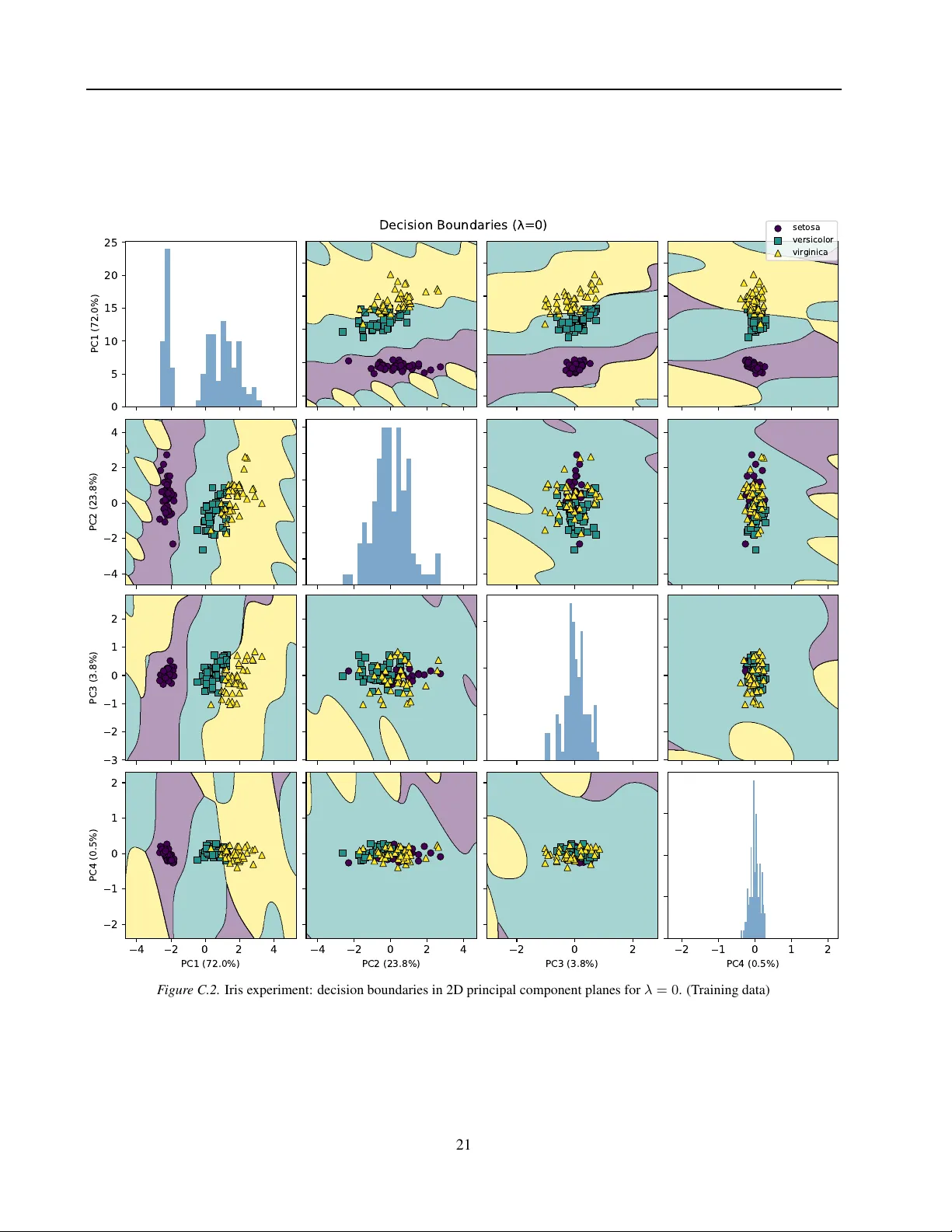
Lipschitz veriﬁcation of neural netw orks thr ough training Simon Kuang 1 Y uezhu Xu 2 S. Sivaranjani 2 Xinfan Lin 1 Abstract The global Lipschitz constant of a neural net- work gov erns both adv ersarial robustness and gen- eralization. Con ventional approaches to “certi- ﬁed training” typically follo w a train-then-verify paradigm: the y train a network and then attempt to bound its Lipschitz constant. Because the ef- ﬁcient “trivial bound” (the product of the layer- wise Lipschitz constants) is exponentially loose for arbitrary networks, these approaches must rely on computationally expensiv e techniques such as semideﬁnite programming, mixed-inte ger pro- gramming, or branch-and-bound. W e propose a different paradigm: rather than designing com- plex veriﬁers for arbitrary networks, we design networks to be veriﬁable by the fast tri vial bound. W e show that directly penalizing the trivial bound during training forces it to become tight, thereby effecti vely re gularizing the true Lipschitz con- stant. T o achiev e this, we identify three structural obstructions to a tight tri vial bound (dead neu- rons, bias terms, and ill-conditioned weights) and introduce architectural mitigations, including a nov el notion of norm-saturating polyactiv ations and bias-free sinusoidal layers. Our approach av oids the runtime complexity of adv anced veriﬁ- cation while achieving strong results: we train ro- bust netw orks on MNIST with Lipschitz bounds that are small (orders of magnitude lower than comparable works) and tight (within 10% of the ground truth). The experimental results v alidate the theoretical guarantees, support the proposed mechanisms, and extend empirically to div erse activ ations and non-Euclidean norms. 1 Department of Mechanical and Aerospace Engineering, Uni- versity of California, Da vis 2 Edwardson School of Industrial En- gineering, Purdue Uni versity . Correspondence to: Simon Kuang < slku@ucdavis.edu > . Pr eprint. Mar ch 31, 2026. 1. Introduction Some neural networks that minimize a loss function on training data are found to underperform on unseen inputs; others perform well on the whole population, but can be eas- ily fooled by imperceptibly small adversarial perturbations. A network may elev ate a small variation (sampling error , inﬁnitesimal distribution shift) abov e true features in the data. A recent hypothesis ( Sze gedy et al. , 2014 ) supported by learning theory ( Bartlett et al. , 2017 ; Neyshab ur et al. , 2015b ; Golowich et al. , 2018 ; Neyshabur et al. , 2018 ) ex- plains both failure modes in terms of the Lipschitz constant. The Lipschitz constant, deﬁned as the maximum change in output per unit change in input, is a nonnegativ e scalar that quantiﬁes the network’ s power to amplify and discrimi- nate relev ant features in the training population—a desirable trait—and its tendency to behav e erratically on unseen or out-of-distribution inputs—an undesirable trait. It follows that the global Lipschitz constant ought to be simultane- ously as large as necessary and as small as possible. This tradeoff has traditionally been captured in mathematical programming by the support vector machine and lasso (for linear models), and by regularized kernel methods (for lo w- dimensional nonlinear models). The former objectiv e of this tradeoff (as lar ge as necessary) is easily captured by a loss function. The latter objecti ve has prov en more elusi ve. It stands to reason that before claiming that a network’ s Lipschitz constant is small, we ﬁrst need to ﬁnd out its value. But the exact Lipschitz constant of a neural network is NP-hard to compute in general ( V irmaux & Scaman , 2018 ), and algorithms are only known for piece- wise linear activ ations such as ReLU ( Jordan & Dimakis , 2020 ; Bhowmick et al. , 2021 ). Consequently , we must rely on upper bounds. A range of methods for upper-bounding the Lipschitz constant ex- ploit information such as the monotonicity of the activ ation function or the compact ranges of hidden layers. These tech- niques include semideﬁnite programming (SDP) ( Fazlyab et al. , 2019 ; Xu & Siv aranjani , 2024 ; 2025 ), polynomial optimization ( Chen et al. , 2020 ), interval arithmetic ( Zhang et al. , 2018 ; 2019 ), and operations research methods ( Ente- sari et al. , 2023 ; Shi et al. , 2025 ). These occupy a spectrum of tradeof fs between conserv atism and runtime complexity . 1 Lipschitz veriﬁcation of neural networks thr ough training At one extreme, one can quickly bound the Lipschitz con- stant of the network by multiplying the Lipschitz constants of the layers ( V irmaux & Scaman , 2018 , Prop. 1); we de- note this the trivial bound (after Xu & Siv aranjani 2024 ). A priori , the trivial bound appears to increase exponentially with netw ork depth and is therefore liable to extreme conser- vat ism ( Szegedy et al. , 2014 ; W eng et al. , 2018 ; Leino et al. , 2021 ). Experimental evidence for this thesis ranges from drastic— 10 2 ( Zhang et al. , 2018 , Figure 3)—to g alactic—in excess of 10 20 ( Fazlyab et al. , 2019 , Figure 2b). There are sev eral schools of thought on ho w to balance “as large as necessary” and “as small as possible. ” Some works impose a hard Lipschitz constraint in training, either as a projection operator in the training loop ( Xu & Siv aranjani , 2023 ; Rev ay et al. , 2024 ; Gouk et al. , 2021 ; Junnarkar et al. , 2024 ) or by a parameterization whose range lies within the Lipschitz cylinder ( W ang & Manchester , 2023 ). Other works promote Lipschitz continuity indirectly by adding a Lipschitz penalty to the loss function ( Pauli et al. , 2021 ; Bungert et al. , 2021 ; Huang et al. , 2021 ). All of these methods are computationally expensiv e and impose extra parameters, hyperparameters, mathematical programs, or subroutines because they access the Lipschitz constant via sophisticated techniques such as semideﬁnite programming. They assume that these techniques are necessary because the tri vial bound is too loose for v eriﬁcation and therefore too restricti v e for training. (W e respond in detail to dif ferent versions of this ar gument in Appendix A .) Our work challenges this popular assumption. W e admit that the tri vial bound is unacceptably loose for a general neural network. But as we show in Section 3.2 , so is the SDP bound. Because “verifying robustness for arbitrary neural networks is hard, ” Raghunathan et al. ( 2018 ) call for training “neural networks that are amenable to veriﬁcation, in the same way that it is possible to write programs that can be formally veriﬁed. ” Surprisingly , the trivial bound is ﬁt for this purpose. As we show by theory in Section 3.3 and example in Section 5 , the trivial bound becomes tight when it is penalized in training. Lipschitz regularization then regulates the true Lipschitz constant of the network. Instead of designing the veriﬁcation subtask for an arbitrary neural netw ork, our approach is to design the network architecture and loss function in order to be veriﬁable by the tri vial Lipschitz bound. Related work (rob ustness) A small global Lipschitz con- stant guarantees that within a ball of radius in versely propor - tional to the Lipschitz constant, the classiﬁer is indif ferent to perturbations. Some other regularizers ( Hoffman et al. 2019 ; Nenov et al. 2024 ; Y oshida & Miyato 2017 , among others) impose a similar inductiv e bias tow ards smoothness, but do not come with a guarantee. Local Lipschitz bounds ( Jordan & Dimakis , 2020 ; Bho wmick et al. , 2021 ; Xu & Siv aranjani , 2025 ) and other forms of rob ustness certiﬁcates ( Raghunathan et al. , 2018 ; W ong & Kolter , 2018 ; Lee et al. , 2020 ) offer guarantees on a “pointwise, ” per-instance basis by introspection of the network’ s weights, given kno wledge of the input and attack parameters. Rather, global Lipschitz bounds are “uniform” and apply to all inputs and all attacks, and impose a constant cost at inference time. Contributions W e attribute the looseness of the triv- ial bound to three causes: dead neurons, biases, and ill- conditioned weight matrices. W e then mitigate them at the lev el of architecture and loss function (rather than over - come them in downstream analysis) with polyacti v ations, a novel vector -v alued activ ation architecture designed to saturate norm bounds; sinusoidal activ ation layers that do not need biases to be uni versal approximators; and direct penalization of the trivial Lipschitz bound. W e verify these mitigations and their theoretical backing experimentally on a range of networks and datasets (Iris, Section 5.1 ; MNIST , Section 5.2 ). Empirically , we ﬁnd orders-of-magnitude im- prov ements to the trivial bound that bring it to within a factor of 1–2 of the true Lipschitz constant. W e also ﬁnd support for the theoretical mechanisms behind these im- prov ements, such as an argument by matrix factorization that Lipschitz regularization leads to well-conditioned ma- trices. W e show that these empirical results translate to acti- vation functions ranging from specialized to con ventional, and to non-Euclidean norms. W e demonstrate the performance of this approach by train- ing a neural network with cross-entropy loss to 98% on MNIST and certifying that its Lipschitz constant lies be- tween 5.5 and 6. This is a remarkable achie vement because: 1. It is relatively rare in the vast literature on Lipschitz analysis to ground-truth against lo wer bounds. 1 2. Our network’ s Lipschitz upper bound is signiﬁcantly smaller than other estimates for networks with com- parable performance, whose Lipschitz upper bounds range from 50 to 500 ( Fazlyab et al. , 2019 , Fig. 2a). 3. The training consists of minimizing a loss function (namely , a data loss plus the trivial Lipschitz bound) using a black-box ﬁrst-order optimizer . 4. The veriﬁcation method is like wise elementary: it con- sists of multiplying induced norms of weight matrices to obtain an upper bound, and locally searching for a secant vector that attains the Lipschitz constant to obtain a lower bound. 1 W ang & Manchester ( 2023 ) also compares to empirical lower bounds on a 1D toy problem. Jordan & Dimakis ( 2020 ); Bhowmick et al. ( 2021 ); Sbihi et al. ( 2024 ) compute lower bounds in super- polynomial time. 2 Lipschitz veriﬁcation of neural networks thr ough training 2. Preliminaries The vector of ones is 1 . The ℓ p norm of x ∈ R d is deﬁned by ∥ x ∥ p =   d X i =1 | x i | p   1 /p , p ∈ [1 , ∞ ); ∥ x ∥ ∞ = max i ∈ [ d ] | x i | , p = ∞ . The induced operator p -norm of a matrix A ∈ R d × d is deﬁned by ∥ A ∥ p = max ∥ x ∥ p =1 ∥ Ax ∥ p . The Lipschitz constant of an absolutely continuous function f : R n → R m in the p -norm is ∥ f ∥ Lip ,p = sup x ∈ R n   ∇ f ( x )   p . W e may omit the subscript when p = 2 . A traditional feed-forward neural network of depth L is deﬁned recursiv ely by x 0 = x and x ℓ = σ ℓ  W ℓ x ℓ − 1 + b ℓ  , ℓ = 1 , . . . , L, (1) where σ ℓ acts elementwise and W ℓ and b ℓ are the weights and biases of layer ℓ . W e write f ( x ) = x L . Because in- duced matrix norms are submultiplicati ve, the trivial bound on the Lipschitz constant of a feed-forward network is ∥ f ∥ Lip ,p ≤ L Y ℓ =1    σ ℓ    Lip ,p    W ℓ    p . For z ∈ R n , deﬁne Sin( z ) = diag (sin( z )) and Cos( z ) = diag(cos( z )) . If A is a matrix, Diag( A ) is the diagonal matrix with the same diagonal entries as A and zeros else where. The condition number of a (rectangular) matrix is the ratio of its largest singular v alue to its smallest nonzer o singular value. 3. Mitigating weaknesses of the trivial bound This section presents a stylized narrative of three phenomena underlying the looseness of the trivial Lipschitz bound. For each phenomenon, we construct a toy model that inﬂates the trivial Lipschitz bound and propose an architecture- and/or loss-lev el mitigation moti v ated by theoretical analysis. The purpose is to advocate for a single gold-standard architecture for shallow netw orks—cosine/sine acti v ations trained with a straightforward penalty on the trivial Lipschitz bound— and to raise questions for empirical inv estigation on deeper networks. 3.1. Dead neurons Popular acti vation functions such as ReLU and hyperbolic tangent hav e re gions with little v ariation. A ReLU preacti- vation h may be biased into its negati ve region across the entire training set; thus, a unit such as ReLU(1000 h ) may become positi ve at test time (e.g., under distribution shift). In such a case, the unit’ s Lipschitz constant is 1000, even though this steep slope may be irrele vant (or harmful) to out-of-sample performance. Dead neurons can also result from deeper structures such as the mapping x 7→ z giv en by z = ReLU( − 1000 y ) , y = ReLU(1000 x ) . In this case, the tri vial bound equals 1 million, b ut the true Lipschitz constant is 0, because the argument of the second layer’ s ReLU is nonpositive for every x . In general, com- puting tight neuron ranges is computationally intractable ( W eng et al. , 2018 ; Shi et al. , 2022 ; Jordan & Dimakis , 2020 ; Chen et al. , 2020 ; V irmaux & Scaman , 2018 ). W e mitigate this issue by using polyactiv ations that saturate the Lipschitz constraint without vanishing slopes. 3 . 1 . 1 . P O L Y A C T I V ATI O N S Merely adding a residual bypass to a dead neuron is not sufﬁcient from the perspecti ve of the Lipschitz bound, since layer bounds (1 + ∥ W ∥ p ) would lead to a tri vial bound that grows e xponentially in depth ( Gouk et al. , 2021 ). Some existing w ork on Lipschitz training replaces neuron- lev el nonlinearities with whole-layer nonlinearities such as GroupSort, whose Jacobian is orthogonal ev erywhere on its domain ( Anil et al. , 2019 ). 2 Our approach is closer to CReLU, which maps each input coordinate through multiple activ ations, ensuring that not all channels vanish simultane- ously ( Shang et al. , 2016 ). Deﬁnition 3.1 (Polyacti v ation) . A polyacti v ation function of order K is a tuple of functions { σ k : R → R } K k =1 that acts on vectors by  σ : R d → R dK , x 7→ ( σ 1 ( x ) , σ 2 ( x ) , . . . , σ K ( x )) . Polyactiv ations fan out by a factor of K and are contracted by a wide weight matrix. 3 The Jacobian of a polyactiv ation 2 W e note in passing that the neuron-level absolute v alue activ a- tion function also possesses this property . 3 As the contribution of an y neuron to the next layer’ s neurons is a weighted sum of basis functions, this architecture can be recognized as a K olmogorov-Arnold e xpansion ( Liu et al. , 2025 ). 3 Lipschitz veriﬁcation of neural networks thr ough training layer is ∂ ∂ x  σ ( x ) =       diag σ ′ 1 ( x ) diag σ ′ 2 ( x ) . . . diag σ ′ K ( x )       ∈ R dK × d . Next we formalize a notion under which a polyactiv ation function is “maximally” Lipschitz in the p -norm. Deﬁnition 3.2 (Saturated polyactiv ation) . A polyactiv ation function { σ k } K k =1 is Lipschitz-saturated in the p -norm if  σ has local Lipschitz constant 1 in ev ery neighborhood of R d , or equiv alently , for almost every x ∈ R , K X k =1   σ ′ k ( x )   p = 1 , if p ∈ [1 , ∞ ); ∀ k ∈ [ K ] ,   σ ′ k ( x )   = 1 , if p = ∞ . A saturated polyactiv ation is evidently strictly more e xpres- siv e than a single activ ation function, as it can represent a richer class of functions while maintaining the same Lip- schitz constraint. The idea of saturated polyactiv ations is to maximize the overall representational po wer while main- taining control ov er the Lipschitz bound. Example 1. The absolute value activation function x 7→ | x | is a ﬁrst-or der polyactivation that saturates the p -norm Lipschitz constant for all p ∈ [1 , ∞ ] . Example 2. The ReLU activation x 7→ max(0 , x ) is not sat- urated because its derivative is either 0 or 1. However , the CReLU ( Shang et al. , 2016 ) x 7→ (max(0 , x ) , max(0 , − x )) is a second-or der polyactivation that saturates the Lips- chitz bound for p ∈ [1 , ∞ ) . A variation that saturates the ∞ -norm Lipschitz constant is x 7→ ( x, | x | ) . Example 3. The hyperbolic tangent activation function can be augmented to saturate the 1-norm Lipsc hitz constant by the second-or der polyactivation x 7→ ( x, x − tanh( x )) T o saturate the 2-norm Lipsc hitz constant, one could opt for the thir d-or der polyactivation x 7→ (tanh( x ) , sech( x ) , log cosh( x )) . Example 4. The sine activation function can be augmented to saturate the 2-norm Lipschitz constant by the second- or der polyactivation x 7→ (cos x, sin x ) . 3.2. Biases Equation ( 1 ) is not the only way to write the composition activ ation σ ℓ ◦ shift b ℓ ◦ linear W ℓ ◦ activ ation σ ℓ − 1 ◦ shift b ℓ − 1 ◦ linear W ℓ − 1 ◦ . . . where activ ation denotes the elementwise activ ation, shift denotes translation by the bias, and linear denotes matrix multiplication by the weights. T aking circular permutations, we see that there are three ways to associate these opera- tions: a ctiv ation ◦ s hift ◦ l inear , (ASL) s hift ◦ l inear ◦ a ctiv ation , and (SLA) l inear ◦ a ctiv ation ◦ s hift . (LAS) Theorem 3.3. The trivial Lipschitz bound in the p -norm is tight for ASL units with generic W ∈ R d × d and b ∈ R d , and for SLA and LAS units with arbitrary W ∈ R d × d and b ∈ R d . Howe ver , if we consider the quadruple composition l inear ◦ a ctiv ation ◦ s hift ◦ l inear , (LASL) then the trivial Lipschitz bound in the p -norm can be seen to be arbitrarily loose for LASL units x 7→ W 1 σ ( W 0 x + b ) , as we see from three different explicit constructions. The case of LASL is interesting because it is the prototypical multilayer perceptron used in the classical proof of uni versal approximation by approximate identities. Theorem 3.4. F or both the ReLU and tanh activation func- tions, there exist LASL units R → R d → R on which the trivial 2-Lipschitz bound is Ω( d ) , but the true 2-Lipschitz constant rang es fr om O (1) to Ω( d ) by varying only the biases. Theorem 3.5. F or the sin activation function, ther e exist LASL units R → R 2 d → R on which the trivial Lipschitz bound is Ω( d ) , but the true Lipsc hitz constant is 0. Remark 3.6 . These constructions show that not only the tri vial bound, b ut also any Lipschitz bound which ignores the biases cannot help but impute to the biases their worst-case val ues, and is therefore liable to up to Ω( d ) conserv atism per layer on ReLU and tanh networks, and inﬁnite conserv atism on sinusoidal networks. ( Fazlyab et al. , 2019 ; V irmaux & Scaman , 2018 ; Xu & Siv aranjani , 2024 ). W e mitigate this issue by using a speciﬁc polyactiv ation structure that allows biases to be analytically absorbed into the weight matrices, thereby pre venting the cancellation that loosens the bound. 3 . 2 . 1 . R E C TA N G U L A R S I N U S O I DA L L AY E R S In § 3.2 , we saw that the tri vial bound can be loose because biases in an LASL unit can induce cancellation. What can be done? Removing the s hift parameter from LA S L units would eliminate some slack in the trivial bound, but at the expense of uni v ersal approximation. The criterion for mitigating this weakness is a dimension- independent guarantee that the bound can be sharp for LASL 4 Lipschitz veriﬁcation of neural networks thr ough training units. W e contribute such a guarantee in the 2-norm using the (cos , sin) polyacti vation. Let a LASL unit R r → R n → R m be deﬁned by x 7→ A cos( W x + b ) + B sin( W x + b ) , where A, B ∈ R m × n , W ∈ R n × r , and b ∈ R n . The ke y observ ation is that we can set b = 0 by absorbing the bias into the weight matrices via trigonometric iden- tities (recall that Sin( z ) = diag(sin( z )) and Cos( z ) = diag(cos( z )) ): A 7→ A Cos( b ) − B Sin( b ) B 7→ A Sin( b ) + B Cos( b ) This immediately rules out the adversarial biasing in Theo- rem 3.5 , which relied on the identity sin x + sin( x + π ) = 0 . Now the LASL unit becomes x 7→ A cos( W x ) + B sin( W x ) , (2) and its trivial Lipschitz bound in the 2-norm is     A B     2 ∥ W ∥ 2 . (3) 3.3. Ill-conditioned weight matrices A network with ill-conditioned weight matrices can be less Lipschitz than it appears. This occurs when a neural network contains ill-conditioned subnetworks that cancel out. Owing to the univ ersal approximation property of neural networks, it sufﬁces to make the point using two toy examples: the ReLU and linear activ ation functions. The ReLU acti v ation function is 1-homogeneous: for all α ∈ R × , ReLU( αx ) = α ReLU( x ) . This means that if Λ is an in v ertible diagonal matrix, then any two consecuti ve lay- ers can be reparameterized ( W 0 , W 1 ) 7→ (Λ − 1 W 0 , W 1 Λ) , while the composite function W 1 ReLU( W 0 x + b 0 ) + b 1 = W 1 Λ ReLU(Λ − 1 W 0 x + Λ − 1 b 0 ) + b 1 remains unchanged; this fact has been applied in an- other context to improve the training of ReLU networks ( Neyshab ur et al. , 2015a ; 2016 ). Giv en generic weight ma- trices W 0 , W 1 , reparameterization by Λ = diag( λ, 1 , 1 , 1 , . . . ) , λ → ∞ results in a tri vial Lipschitz bound of Θ( λ ) times the original Lipschitz constant. (The weight matrices’ condition number is also Θ( λ ) .) This form of ill-conditioning also ev ades analysis methods such as LipSDP-Layer ( Fazlyab et al. , 2019 ), which do not kno w the homogeneity of ReLU. W e record this observation as: Theorem 3.7. Given any ReLU network, ther e exists a closed-form, mathematically equivalent network whose triv- ial 2-norm Lipschitz bound is arbitr arily lar ge . It is easy to devise examples which make the tri vial 2-norm Lipschitz bound look bad. That does not mean it is always bad. Next, let us consider the problem of learning an in vertible linear function as a deep neural network with linear activ a- tion function σ ( x ) = x . This is a partly linearized ( Nam et al. , 2025 ) model of an ov erparameterized deep network. W ithout loss of generality , the objective is to learn the iden- tity function using the mapping x 7→ W L W L − 1 · · · W 1 x (4) where the parameters W 1 , W 2 , . . . , W L are square matrices. Theorem 3.8. Consider a deep network ( 4 ) with lin- ear activations and parameter matrices constrained by W L W L − 1 · · · W 1 = I . Let K = ∥ W 1 ∥ 2 ∥ W 2 ∥ 2 · · · ∥ W L ∥ 2 be the trivial Lipschitz bound. Then the following are equiv- alent: 1. K = 1 , i.e. there is no conservatism in the trivial bound. 2. W 1 , W 2 , . . . , W L minimize K subject to W L W L − 1 · · · W 1 = I . 3. The condition number of each par ameter matrix is 1. In this toy example, minimizing the tri vial Lipschitz bound ov er unconstrained degrees of freedom on a le vel set of the loss function recov ers the ground truth Lipschitz constant. 3 . 3 . 1 . L I P S C H I T Z P E N A L T Y Plausibly , this principle generalizes to nonlinear σ and would suggest that well-conditioned neural parameteriza- tions on which the tri vial bound is tight can be reached by continuous optimization, which is hard in theory and easy in practice. Therefore, we propose to train networks onto the Pareto fron- tier of lo w loss and lo w tri vial Lipschitz bound, by choosing polyacti vations that saturate the p -norm and solving a penal- ized optimization problem such as minimize { W ℓ } L ℓ =1 ℓ ( W 1 , . . . , W L ) + λ L Y ℓ =1    W ℓ    p , where ℓ is a data loss function such as neg ativ e log- likelihood o ver the training set and λ > 0 is a tuning param- eter . 5 Lipschitz veriﬁcation of neural networks thr ough training 4. Theoretical and practical lo wer bounds The literature on Lipschitz constant veriﬁcation of neural networks uses “tightness” to refer to metrics such as the ratio of the global Lipschitz constant to the tri vial bound ( Fazlyab et al. , 2019 ; Xu & Si v aranjani , 2024 ). But in the plain mathematical sense, a tight upper bound must be close to the ground truth. Because it is intractable to compute the true Lipschitz constant, we instead compute lower bounds and use the inequality 1 ≤ tightness = Lipschitz upper bound Lipschitz ground truth ≤ Lipschitz upper bound Lipschitz lower bound to show that our Lipschitz upper bounds, in spite of their simplicity , are effecti ve approximations of the ground truth. When considering only a LASL unit equipped with (cos , sin) and absolute value activ ations, we can deriv e lower bounds by pro ving that the Jacobian of the network is large “on a verage. ” (Theorem B.1 adv ances a similar claim for the absolute value acti vation.) Theorem 4.1 (Lo wer bound on sinusoidal networks) . Let f ( x ) be an LASL unit fr om R n → R n → R m given by Equation ( 2 ) , f ( x ) = A cos( W x ) + B sin( W x ) . Then, if W has full rank, the following Lipschitz lower bound holds: ∥ f ∥ 2 Lip , 2 ≥ 1 2 λ max  A Diag ( W W ⊺ ) A ⊺ + B Diag ( W W ⊺ ) B ⊺  , and the trivial Lipschitz bound K =     A B     2 ∥ W ∥ 2 is off by less than a factor of √ 2 κ ( W ) : 1 √ 2 κ ( W ) K ≤ ∥ f ∥ Lip , 2 ≤ K, wher e κ ( W ) = p λ max ( W W ⊺ ) /λ min ( W W ⊺ ) is the con- dition number . The proof appeals to the probabilistic method to ﬁnd an input with a typical Jacobian norm. A key cancellation step uses the fact that because these activ ations ha ve slopes ranging from -1 to 1; a similar method would not work for ReLU or tanh (0 to 1). In deeper networks, it is harder to get a lower bound on the Jacobian. Howe ver , we can still use the probabilistic method ov er an ensemble of random netw orks to calculate the exact second moment of the Jacobian. This is weaker in that it is an average-case bound and only applies to the random initialization (which is quickly departed in training), but it is strong in that it holds with equality , pointwise in x . The random-phase initialization of ( A, B ) ∈ R d × d ′ at scale α is deﬁned as  A B  =  ¯ A ¯ B   Cos( θ ) − Sin( θ ) Sin( θ ) Cos( θ )  , (5) where ¯ A, ¯ B ∈ R d × d ′ are i.i.d. Gaussian with variance α/d ′ , and θ is uniformly distributed on the torus ( R / 2 π Z ) d . Informal Theorem (Theorem B.2 ) . Let f be a (cos , sin) neural network of depth L and arbitrary width, initialized with random phases at scale α . E  D f ( x ) D f ( x ) ⊺  = α L I for every input x . The idea of this proof is that the random phases 4 decorrelate the weights across layers, leading to a diagonal cov ariance structure. As a by-product, we have also established an exact stable initialization for sinusoidal networks ( Sitzmann et al. , 2020 ). The choice α = 1 stabilizes the av erage slope of the net- work; the choice α = 2 − 1 / 2 corresponding to the Kaiming initialization stabilizes the worst case ( He et al. , 2015 ). This discrepancy reﬂects that at initialization, the trivial Lipschitz constant is loose by a factor of √ 2 per layer; it is the role of training to close this gap. 4.1. An empirical bound In experiments, we obtain an empirical lower bound b L by locally maximizing the secant slope ∥ f ∥ Lip , 2 ≤ b L ≈ m ax x,y   f ( x ) − f ( y )   2 ∥ x − y ∥ 2 + ϵ , using ϵ = 10 − 8 and reporting the best of twenty runs of L-BFGS, initialized with x and y sampled from the training data. It is ﬁtting that the network’ s highest local variation should be attained on a line segment between training points, where the data loss function opposes the do wnward pressure on the Jacobian imposed by Lipschitz regularization. 5. Experimental results W e carry out numerical experiments at varying scales to address the follo wing questions, which are left unresolv ed by our theoretical analysis. 4 The random phases, which anti-correlate the fourth moments of the weights while lea ving the second moments unchanged, do not hav e noticeable consequences for practical training. 6 Lipschitz veriﬁcation of neural networks thr ough training T able 5.1. Iris experiment: ﬁnal predictiv e performance after 20,000 steps. λ T rain Loss T est Loss T rain Acc. T est Acc. 0 1 . 0 × 10 − 4 0 . 4661 1 . 000 0 . 933 10 − 2 0 . 0542 0 . 0932 0 . 983 0 . 967 Question 1 (Feasibility) . What is the effect of Lipschitz r e gularization on the trivial bound? Question 2 (T ightness) . What is the effect of Lipsc hitz r e g- ularization on the true Lipschitz constant? Question 3 (Performance) . What is the effect of Lipsc hitz r e gularization on the model ’ s goodness of ﬁt, both in-sample and out-of-sample? Question 4 (Robustness) . How conﬁdently does global Lip- schitz r e gularization certify r obust learning? 5.1. Iris dataset: upper and lower 2-norm Lipschitz bounds on a shallow network This section trains and e valuates a small multilayer percep- tron (detailed in Section C.1 ) with (cos , sin) polyactiv ation on the Iris dataset in order to v alidate Theorem 4.1 . W e opti- mize the penalized objectiv e NLL + λK for λ ∈ { 0 , 10 − 2 } . T o assess tightness, we compare K to (i) the guaranteed lower bound K √ 2 κ ( W ) ≤ ∥ f ∥ Lip , 2 ≤ K, and (ii) the empirical lower bound b L . Results While λ = 0 results in an exploding K , adding the Lipschitz penalty reduces K by more than an order of magnitude (T able 5.2 , Question 1 ). Regularization also makes the tri vial bound essentially tight in practice (T a- ble 5.2 , Question 2 ). Moreover , the Lipschitz upper bound ( K = 5 . 84 ) of the re gularized netw ork is much smaller than the Lipschitz lower bound of the unregularized network ( b L = 105 . 74 ), indicating that the Lipschitz penalty reduces the network’ s true Lipschitz constant. While λ = 0 yields near-perfect interpolation and classical ov erﬁtting, adding the Lipschitz penalty impro ves test loss and slightly improves test accuracy (T able 5.1 , answering Question 3 ). V isually , on two-dimensional slices of the domain, the regu- larized network (Figure C.3 ) e xhibits smoother boundaries than the unregularized network (Figure C.2 ). 5.2. MNIST dataset: Lipschitz bounds This section trains and ev aluates a larger network (detailed in Section C.3 ) on the MNIST dataset in order to v alidate the T able 5.2. Iris experiment: 2-norm Lipschitz upper bound K versus lo wer bounds. Here K/ ( √ 2 κ ( W )) is the guaranteed lower bound from Theorem 4.1 , while b L is an empirical lower bound from local optimization of the Lipschitz ratio ov er input pairs. λ K (upper) K/ ( √ 2 κ ( W )) b L K/ b L 0 179 . 21 25 . 04 105 . 74 1 . 69 10 − 2 5 . 84 0 . 82 5 . 84 1 . 00 0.2 0.4 0.6 0.8 1.0 singular values (nor malized to max) 0 2 4 6 8 10 12 14 16 density = 0 = 0 . 0 1 F igure 5.1. MNIST experiment: normalized singular values of the weight matrices (with and without penalty). claim that the linearized Theorem 3.8 e xtends to nonlinear networks. Results As with the Iris experiment, we ﬁnd that λ = 0 results in an e xploding Lipschitz upper bound, while adding a Lipschitz penalty leads to a reduction by one to two orders of magnitude (T able 5.3 , Figure C.5 , Question 1 ). W e again run a local Lipschitz attack using L-BFGS to ﬁnd a lower bound b L on the global Lipschitz constant, and conclude (T able 5.3 , Question 2 ): 1. Lipschitz regularization reduces the true Lipschitz con- stant of the resulting network by at least ∼ 10 × , by comparing b L of the unregularized network to K of the regularized network, and 2. The trivial Lipschitz upper bound K of the regular - ized network is conserv ati ve by no more than 10%, by comparing it to b L of the same regularized netw ork. While the regularized netw ork has a higher in-sample loss, it has comparable test error: 1 . 70% for λ = 0 versus 1 . 41% 7 Lipschitz veriﬁcation of neural networks thr ough training T able 5.3. MNIST experiment: 2-norm Lipschitz upper bound K versus empirical lo wer bound b L . λ K (upper) b L (lo wer) K/ b L 0 187 . 32 ± 21 . 45 58 . 99 ± 3 . 79 3 . 18 10 − 2 5 . 69 ± 0 . 03 5 . 18 ± 0 . 03 1 . 10 for λ = 10 − 2 (Figure C.4 , Question 3 ). T o quantify the ef fect on rob ustness (Question 4 ), we le vy an ℓ 2 PGD attack on the MNIST test set using 40 pro- jected gradient steps (step size ϵ/ 10 ) for budgets ϵ ∈ { 2 − 1 , 2 − 2 , 2 − 3 , 2 − 4 , 2 − 5 } . The resulting adv ersarial error rates are reported in T able C.1 and plotted in Figure C.4 . The Lipschitz-regularized model substantially reduces adversar - ial error at larger perturbation budgets (e.g., at ϵ = 2 − 1 the error drops from 13 . 04% to 4 . 90% ). It also has tighter robustness certiﬁcates (obtained by comparing classiﬁcation margin to perturbation b udget times Lipschitz bound). W e also ﬁnd empirical evidence for the mechanism modeled by Theorem 3.8 . W e plot the empirical distribution of all singular values of weight matrices, normalized by the max- imum singular value of the same matrix, and ﬁnd that the Lipschitz-regularized networks concentrate their singular value spectra near the maximum singular value (Figure 5.1 ). This supports the claim that penalizing the maximum singu- lar value allo ws the optimizer to train the lower spectrum, to which the operator norm is indifferent. Discussion: tightness In much of the literature on global Lipschitz veriﬁcation of trained networks, a Lipschitz upper bound obtained by advanced methods is considered tight if it compares fa v orably to the tri vial upper bound K ( Fazlyab et al. , 2019 ; Xu & Siv aranjani , 2024 ). Unfortunately , this comparison is not ground-truthed against the true Lipschitz constant of the network. By contrast, our tightness ratio K/ b L upper-bounds the true conservatism of the trivial up- per bound K . Our re gularized MNIST network, like that of Xu & Siv aranjani ( 2025 ), achie ves < 2% test error when training with cross-entropy , but with a global Lipschitz up- per bound of 5 . 69 (T able 5.3 ). This is commensurate with Xu & Siv aranjani ( 2025 )’ s local Lipschitz certiﬁcates at a radius of 2 − 8 , and an order of magnitude smaller than Xu & Siv aranjani ( 2025 )’ s local Lipschitz certiﬁcates at a radius of 2 − 1 . Discussion: r obustness W e enter the quantitativ e “arms race” of robust learning ( Raghunathan et al. , 2018 ), with order-of-magnitude impro vements in the Lipschitz constant. The rob ustness of our Lipschitz-regularized netw ork against PGD attacks is comparable ( ± 1% at each attack radius) to that of Xu & Si v aranjani ( 2025 )’ s MNIST network trained using a sophisticated local Jacobian penalty heuristic ( Hoff- man et al. , 2019 ). The dif ference is that our method is a one-line algorithm with a single tuning parameter λ . Comparisons with other methods Comparisons between our approach and other activ ation functions (Section D.1 ) and penalties (Section D.3 ), and extensions to other Lip- schitz norms (Section D.2 ) are made in the appendix. In summary , we ﬁnd that in deeper networks where Theo- rem 4.1 does not apply , the expressivity and tightness of our method result primarily from optimizing the tri vial bound, with a smaller or ambi v alent contrib ution from the choice of activ ation function. The absolute value acti v ation often has the tightest bounds and best ﬁt; ReLU the loosest bounds and worst ﬁt. Across dif ferent settings, the mechanism of action seems to be that weight matrices are pushed to the corners of induced norm balls: well-conditioned matrices in the 2-norm, equal-ro w-norm matrices in the ∞ -norm, and equal-column-norm matrices in the 1 -norm. W e also make an apples-to-apples comparison to direct pa- rameterization, concluding that enforcing a hard Lipschitz constraint via a semideﬁnite program on a ReLU network is mor e restricti ve than enforcing the same constraint via the trivial bound on an abs netw ork (Section D.4 ). 6. Conclusion W e have shown that the tri vial Lipschitz bound—the prod- uct of layerwise Lipschitz constants—can be made tight by design, rather than loose by default. W e exploit ov er- parameterization as an ally in this endea v or , as it pro vides the ﬂexibility to optimize the tri vial bound while maintain- ing expressivity . Our methodology does not require any new data structures, algorithms, or subroutines: it can be implemented as a single penalty term with a single hyperpa- rameter . By aligning the training objectiv e with the veriﬁcation method, we can obtain networks that are expressi ve, rob ust, and certiﬁable. 8 Lipschitz veriﬁcation of neural networks thr ough training Impact Statement This paper presents work whose goal is to advance the ﬁeld of Machine Learning. There are many potential societal consequences of our work, none which we feel must be speciﬁcally highlighted here. Reproducibility Statement The results can be reproduced by running the Jupyter note- books included in lipschitz.zip . References Anil, C., Lucas, J., and Grosse, R. Sorting Out Lipschitz Function Approximation. In Chaudhuri, K. and Salakhut- dinov , R. (eds.), Pr oceedings of the 36th International Confer ence on Mac hine Learning , volume 97 of Pr oceed- ings of Machine Learning Researc h , pp. 291–301. PMLR, June 2019. Bartlett, P . L., Foster , D. J., and T elgarsky , M. Spectrally- normalized margin bounds for neural networks. In Pr o- ceedings of the 31st International Conference on Neu- ral Information Pr ocessing Systems , NIPS’17, pp. 6241– 6250, Red Hook, NY , USA, 2017. Curran Associates Inc. ISBN 978-1-5108-6096-4. ev ent-place: Long Beach, California, USA. Bhowmick, A., D’Souza, M., and Raghavan, G. S. Lip- BaB: Computing Exact Lipschitz Constant of ReLU Networks. In Farka ˇ s, I., Masulli, P ., Otte, S., and W ermter , S. (eds.), Artiﬁcial Neural Networks and Ma- chine Learning – ICANN 2021 , pp. 151–162, Cham, 2021. Springer International Publishing. ISBN 978-3- 030-86380-7. doi: 10.1007/978-3-030-86380-7 13 . Bungert, L., Raab, R., Roith, T ., Schwinn, L., and T en- brinck, D. CLIP: Cheap Lipschitz training of neural net- works. In International Confer ence on Scale Space and V ariational Methods in Computer V ision , pp. 307–319. Springer , 2021. B ´ ethune, L. Deep learning with Lipschitz constraints . Theses, Uni versit ´ e de T oulouse, February 2024. Issue: 2024TLSES014. Chen, T ., Lasserre, J. B., Magron, V ., and P auwels, E. Semi- algebraic Optimization for Lipschitz Constants of ReLU Networks. In Larochelle, H., Ranzato, M., Hadsell, R., Balcan, M. F ., and Lin, H. (eds.), Advances in Neural Information Pr ocessing Systems , volume 33, pp. 19189– 19200. Curran Associates, Inc., 2020. Cisse, M., Bojanowski, P ., Grave, E., Dauphin, Y ., and Usunier , N. Parse v al Networks: Improving Rob ustness to Adversarial Examples. In Precup, D. and T eh, Y . W . (eds.), Pr oceedings of the 34th International Conference on Machine Learning , v olume 70 of Pr oceedings of Ma- chine Learning Resear ch , pp. 854–863. PMLR, 2017. Dubach, R., Abdallah, M. S., and Poggio, T . Multiplicative Regularization Generalizes Better Than Additiv e Regular - ization. Article, Center for Brains, Minds and Machines (CBMM), July 2025. Accepted: 2025-07-02T20:03:52Z. Entesari, T ., Shariﬁ, S., and Fazlyab, M. ReachLipBnB: A branch-and-bound method for reachability analysis of neural autonomous systems using Lipschitz bounds. In 2023 IEEE International Conference on Robotics and Automation (ICRA) , pp. 1003–1010, May 2023. doi: 10.1109/ICRA48891.2023.10160732 . Fazlyab, M., Robe y , A., Hassani, H., Morari, M., and Pap- pas, G. Efﬁcient and Accurate Estimation of Lipschitz Constants for Deep Neural Networks. In Advances in Neural Information Pr ocessing Systems , volume 32. Cur- ran Associates, Inc., 2019. Golowich, N., Rakhlin, A., and Shamir, O. Size- Independent Sample Complexity of Neural Networks. In Bubeck, S., Perchet, V ., and Rigollet, P . (eds.), Pr o- ceedings of the 31st Confer ence On Learning Theory , v ol- ume 75 of Proceedings of Machine Learning Resear ch , pp. 297–299. PMLR, 2018. Gouk, H., Frank, E., Pfahringer, B., and Cree, M. J. Reg- ularisation of neural networks by enforcing Lipschitz continuity . Machine Learning , 110(2):393–416, February 2021. ISSN 0885-6125, 1573-0565. doi: 10.1007/s10994- 020-05929-w . He, K., Zhang, X., Ren, S., and Sun, J. Delving Deep into Rectiﬁers: Surpassing Human-Lev el Performance on ImageNet Classiﬁcation. In 2015 IEEE International Confer ence on Computer V ision (ICCV) , pp. 1026–1034, December 2015. doi: 10.1109/ICCV .2015.123 . ISSN: 2380-7504. Hoffman, J., Roberts, D. A., and Y aida, S. Robust Learning with Jacobian Regularization, August 2019. arXiv:1908.02729 [stat]. Huang, Y ., Zhang, H., Shi, Y ., K olter , J. Z., and Anandku- mar , A. T raining certiﬁably rob ust neural networks with efﬁcient local lipschitz bounds. In Advances in Neural Information Pr ocessing Systems , volume 34, pp. 22745– 22757, 2021. Jordan, M. and Dimakis, A. G. Exactly Computing the Local Lipschitz Constant of ReLU Networks. In Larochelle, H., Ranzato, M., Hadsell, R., Balcan, M. F ., and Lin, H. (eds.), Advances in Neural Information Pr ocessing Systems , volume 33, pp. 7344–7353. Curran Associates, Inc., 2020. 9 Lipschitz veriﬁcation of neural networks thr ough training Junnarkar , N., Arcak, M., and Seiler , P . Synthesizing Neu- ral Network Controllers with Closed-Loop Dissipati vity Guarantees, April 2024. arXiv:2404.07373 [cs, eess]. Lai, B.-H., Huang, P .-H., Kung, B.-H., and Chen, S.-T . En- hancing Certiﬁed Rob ustness via Block Reﬂector Orthog- onal Layers and Logit Annealing Loss. In F orty-second International Confer ence on Machine Learning , 2025. Lee, S., Lee, J., and Park, S. Lipschitz-certiﬁable training with a tight outer bound. In Advances in Neural Informa- tion Pr ocessing Systems , volume 33, pp. 16891–16902, 2020. Leino, K., W ang, Z., and Fredrikson, M. Globally-robust neural networks. In International Confer ence on Machine Learning , pp. 6212–6222. PMLR, 2021. Liu, Z., W ang, Y ., V aidya, S., Ruehle, F ., Halverson, J., Soljacic, M., Hou, T . Y ., and T egmark, M. KAN: K ol- mogorov–Arnold Networks. In The Thirteenth Interna- tional Confer ence on Learning Repr esentations , 2025. Miyato, T ., Kataoka, T ., K oyama, M., and Y oshida, Y . Spec- tral Normalization for Generati ve Adv ersarial Networks. In International Confer ence on Learning Repr esentations , 2018. Nam, Y ., Lee, S. H., Domin ´ e, C. C. J., Park, Y ., London, C., Choi, W ., G ¨ oring, N. A., and Lee, S. Position: Solve Layerwise Linear Models First to Understand Neural Dynamical Phenomena (Neural Collapse, Emergence, Lazy/Rich Regime, and Grokking). June 2025. Nenov , R., Haider , D., and Balazs, P . (Almost) Smooth Sail- ing: T ow ards Numerical Stability of Neural Networks Through Dif ferentiable Regularization of the Condition Number . In 2nd Dif fer entiable Almost Everything W ork- shop at the 41st International Conference on Machine Learning , 2024. Neyshab ur , B., Salakhutdinov , R. R., and Srebro, N. Path- SGD: P ath-Normalized Optimization in Deep Neural Net- works. In Advances in Neural Information Pr ocessing Systems , volume 28. Curran Associates, Inc., 2015a. Neyshab ur , B., T omioka, R., and Srebro, N. Norm-based capacity control in neural networks. In Conference on learning theory , pp. 1376–1401. PMLR, 2015b. Neyshab ur , B., T omioka, R., Salakhutdinov , R., and Sre- bro, N. Data-Dependent Path Normalization in Neural Networks, 2016. eprint: 1511.06747. Neyshab ur , B., Bhojanapalli, S., and Srebro, N. A P AC- Bayesian Approach to Spectrally-Normalized Margin Bounds for Neural Networks. In International Confer - ence on Learning Repr esentations , 2018. Orabona, F . and T ommasi, T . T raining Deep Netw orks with- out Learning Rates Through Coin Betting. In Advances in Neur al Information Pr ocessing Systems , v olume 30. Curran Associates, Inc., 2017. Pauli, P ., K och, A., Berberich, J., Kohler , P ., and Allg ¨ ower , F . T raining rob ust neural networks using Lipschitz bounds. IEEE Contr ol Systems Letters , 6:121–126, 2021. Pub- lisher: IEEE. Raghunathan, A., Steinhardt, J., and Liang, P . Certiﬁed Defenses against Adversarial Examples. February 2018. Rev ay , M., W ang, R., and Manchester , I. R. Recurrent Equilibrium Networks: Flexible Dynamic Models W ith Guaranteed Stability and Rob ustness. IEEE T ransac- tions on Automatic Contr ol , 69(5):2855–2870, May 2024. ISSN 1558-2523. doi: 10.1109/T AC.2023.3294101 . Sbihi, M., Jan, S., and Couellan, N. MIQCQP reformu- lation of the ReLU neural networks Lipschitz constant estimation problem, February 2024. arXi v:2402.01199 [math]. Shang, W ., Sohn, K., Almeida, D., and Lee, H. Under- standing and impro ving conv olutional neural networks via concatenated rectiﬁed linear units. In international confer ence on machine learning , pp. 2217–2225. PMLR, 2016. Shi, Z., W ang, Y ., Zhang, H., K olter , J. Z., and Hsieh, C.-J. Efﬁciently computing local lipschitz constants of neural networks via bound propagation. Advances in Neural Information Pr ocessing Systems , 35:2350–2364, 2022. Shi, Z., Jin, Q., Kolter , Z., Jana, S., Hsieh, C.-J., and Zhang, H. Neural Network V eriﬁcation with Branch- and-Bound for General Nonlinearities, February 2025. arXiv:2405.21063 [cs]. Singla, S., Singla, S., and Feizi, S. Improved deterministic l2 robustness on CIF AR-10 and CIF AR-100. In Interna- tional Confer ence on Learning Repr esentations , 2022. Sitzmann, V ., Martel, J., Bergman, A., Lindell, D., and W et- zstein, G. Implicit Neural Representations with Periodic Acti vation Functions. In Advances in Neural Information Pr ocessing Systems , volume 33, pp. 7462–7473. Curran Associates, Inc., 2020. Szegedy , C., Zaremba, W ., Sutskev er , I., Bruna, J., Erhan, D., Goodfellow , I., and Fer gus, R. Intriguing properties of neural networks, February 2014. arXiv:1312.6199 [cs]. V irmaux, A. and Scaman, K. Lipschitz Regularity of Deep Neural Networks: Analysis and Efﬁcient Estimation. In Bengio, S., W allach, H., Larochelle, H., Grauman, K., Cesa-Bianchi, N., and Garnett, R. (eds.), Advances in 10 Lipschitz veriﬁcation of neural networks thr ough training Neural Information Pr ocessing Systems , volume 31. Cur- ran Associates, Inc., 2018. W ainwright, M. J. High-Dimensional Statistics: A Non- Asymptotic V iewpoint . Cambridge Series in Statisti- cal and Probabilistic Mathematics. Cambridge Univ er- sity Press, Cambridge, 2019. ISBN 978-1-108-49802-9. doi: 10.1017/9781108627771 . W ang, R. and Manchester , I. Direct parameterization of lipschitz-bounded deep networks. In International Con- fer ence on Machine Learning , pp. 36093–36110. PMLR, 2023. W eng, L., Zhang, H., Chen, H., Song, Z., Hsieh, C.-J., Daniel, L., Boning, D., and Dhillon, I. T owards fast computation of certiﬁed robustness for relu networks. In International Conference on Machine Learning , pp. 5276–5285. PMLR, 2018. W ong, E. and K olter , Z. Prov able defenses against adversar- ial e xamples via the con ve x outer adv ersarial polytope. In International confer ence on machine learning , pp. 5286– 5295. PMLR, 2018. Xu, Y . and Siv aranjani, S. Learning Dissipati ve Neural Dynamical Systems. IEEE Contr ol Sys- tems Letters , 7:3531–3536, 2023. ISSN 2475-1456. doi: 10.1109/LCSYS.2023.3337851 . Xu, Y . and Sivaranjani, S. ECLipsE: Ef ﬁcient Composi- tional Lipschitz Constant Estimation for Deep Neural Networks. In Globerson, A., Mackey , L., Belgrave, D., Fan, A., Paquet, U., T omczak, J., and Zhang, C. (eds.), Advances in Neural Information Pr ocessing Systems , vol- ume 37, pp. 10414–10441. Curran Associates, Inc., 2024. Xu, Y . and Siv aranjani, S. ECLipsE-Gen-Local: Efﬁcient Compositional Local Lipschitz Estimates for Deep Neural Networks, October 2025. arXiv:2510.05261 [cs]. Y oshida, Y . and Miyato, T . Spectral Norm Regularization for Improving the Generalizability of Deep Learning, May 2017. arXiv:1705.10941 [stat]. Zhang, H., W eng, T .-W ., Chen, P .-Y ., Hsieh, C.-J., and Daniel, L. Efﬁcient neural network rob ustness certiﬁca- tion with general acti vation functions. Advances in neural information pr ocessing systems , 31, 2018. Zhang, H., Zhang, P ., and Hsieh, C.-J. RecurJac: An Efﬁ- cient Recursiv e Algorithm for Bounding Jacobian Matrix of Neural Networks and Its Applications. Pr oceedings of the AAAI Confer ence on Artiﬁcial Intelligence , 33(01): 5757–5764, July 2019. ISSN 2374-3468, 2159-5399. doi: 10.1609/aaai.v33i01.33015757 . 11 Lipschitz veriﬁcation of neural networks thr ough training Contents 1 Intr oduction 1 2 Pr eliminaries 3 3 Mitigating weaknesses of the trivial bound 3 3.1 Dead neurons . . . . . . . . . . . . . . . . . . . . . . . . . . . . . . . . . . . . . . . . . . . . . . . . . 3 3.1.1 Polyactiv ations . . . . . . . . . . . . . . . . . . . . . . . . . . . . . . . . . . . . . . . . . . . . 3 3.2 Biases . . . . . . . . . . . . . . . . . . . . . . . . . . . . . . . . . . . . . . . . . . . . . . . . . . . . . 4 3.2.1 Rectangular sinusoidal layers . . . . . . . . . . . . . . . . . . . . . . . . . . . . . . . . . . . . 4 3.3 Ill-conditioned weight matrices . . . . . . . . . . . . . . . . . . . . . . . . . . . . . . . . . . . . . . . . 5 3.3.1 Lipschitz penalty . . . . . . . . . . . . . . . . . . . . . . . . . . . . . . . . . . . . . . . . . . . 5 4 Theoretical and practical lower bounds 6 4.1 An empirical bound . . . . . . . . . . . . . . . . . . . . . . . . . . . . . . . . . . . . . . . . . . . . . . 6 5 Experimental r esults 6 5.1 Iris dataset: upper and lo wer 2-norm Lipschitz bounds on a shallow netw ork . . . . . . . . . . . . . . . . 7 5.2 MNIST dataset: Lipschitz bounds . . . . . . . . . . . . . . . . . . . . . . . . . . . . . . . . . . . . . . 7 6 Conclusion 8 A Objections to the trivial bound considered 14 B Supplement to Section 3 15 C Supplement to Section 5 20 C.1 Iris: methodology . . . . . . . . . . . . . . . . . . . . . . . . . . . . . . . . . . . . . . . . . . . . . . . 20 C.2 Iris: results . . . . . . . . . . . . . . . . . . . . . . . . . . . . . . . . . . . . . . . . . . . . . . . . . . 20 C.3 MNIST : methodology . . . . . . . . . . . . . . . . . . . . . . . . . . . . . . . . . . . . . . . . . . . . . 23 C.4 MNIST : results . . . . . . . . . . . . . . . . . . . . . . . . . . . . . . . . . . . . . . . . . . . . . . . . 23 D Additional experiments on MNIST 24 D.1 Other (poly-)activ ations . . . . . . . . . . . . . . . . . . . . . . . . . . . . . . . . . . . . . . . . . . . . 24 D.2 Regularization in p = 1 and p = ∞ . . . . . . . . . . . . . . . . . . . . . . . . . . . . . . . . . . . . . 25 D.3 Other penalties . . . . . . . . . . . . . . . . . . . . . . . . . . . . . . . . . . . . . . . . . . . . . . . . 29 D.4 Comparison to a direct parameterization . . . . . . . . . . . . . . . . . . . . . . . . . . . . . . . . . . . 32 List of Figures 5.1 MNIST experiment: normalized singular values of the weight matrices (with and without penalty). . . . . 7 12 Lipschitz veriﬁcation of neural networks thr ough training C.1 Iris experiment: training curves for λ = 0 (left) and λ = 10 − 2 (right). Shaded area indicates the gap between theoretical upper and lower bounds on the Lipschitz constant. . . . . . . . . . . . . . . . . . . . 20 C.2 Iris experiment: decision boundaries in 2D principal component planes for λ = 0 . (Training data) . . . . 21 C.3 Iris experiment: decision boundaries in 2D principal component planes for λ = 10 − 2 . (T raining data) . . 22 C.4 MNIST experiment: PGD attack success rate (with and without penalty). . . . . . . . . . . . . . . . . . 23 C.5 MNIST experiment: training curves (with and without penalty). . . . . . . . . . . . . . . . . . . . . . . 24 D.1 MNIST experiment: normalized row norms of weight matrices for p = ∞ norm (with and without penalty). 27 D.2 MNIST experiment: normalized column norms of weight matrices for p = 1 norm (with and without penalty). 27 D.3 MNIST experiment: normalized singular v alues of the weight matrices for alternative re gularization methods. 29 D.4 MNIST experiment: PGD attack error rates for alternative re gularization methods. . . . . . . . . . . . . . 30 D.5 MNIST experiment: training curves for alternativ e re gularization methods. . . . . . . . . . . . . . . . . . 31 D.6 MNIST experiment: PGD attack error rates for direct parameterization comparison. . . . . . . . . . . . . 32 D.7 MNIST experiment: training curves for direct parameterization comparison. . . . . . . . . . . . . . . . . 33 List of T ables 5.1 Iris experiment: ﬁnal predictive performance after 20,000 steps. . . . . . . . . . . . . . . . . . . . . . . 7 5.2 Iris experiment: 2-norm Lipschitz upper bound K versus lo wer bounds. Here K/ ( √ 2 κ ( W )) is the guaranteed lower bound from Theorem 4.1, while b L is an empirical lower bound from local optimization of the Lipschitz ratio ov er input pairs. . . . . . . . . . . . . . . . . . . . . . . . . . . . . . . . . . . . . . . 7 5.3 MNIST experiment: 2-norm Lipschitz upper bound K versus empirical lo wer bound b L . . . . . . . . . . . 8 C.1 MNIST experiment: PGD attack error rates (%) at v arious perturbation radii ϵ . . . . . . . . . . . . . . . . 23 D.1 MNIST experiment: PGD attack error rates (%) for various activ ations with Lipschitz regularization ( λ = 10 − 2 ). emp = empirical, cert = certiﬁed. . . . . . . . . . . . . . . . . . . . . . . . . . . . . . . . . 25 D.2 MNIST experiment: Lipschitz bounds and predictiv e performance for v arious acti v ations with Lipschitz regularization ( λ = 10 − 2 ). . . . . . . . . . . . . . . . . . . . . . . . . . . . . . . . . . . . . . . . . . . 25 D.3 MNIST experiment: Lipschitz bounds for p = ∞ norm with various acti v ations. . . . . . . . . . . . . . . 26 D.4 MNIST experiment: Predictive performance for p = ∞ norm with various acti vations. . . . . . . . . . . 26 D.5 MNIST experiment: Lipschitz bounds for p = 1 norm with v arious acti v ations. . . . . . . . . . . . . . . 26 D.6 MNIST experiment: Predictive performance for p = 1 norm with various acti vations. . . . . . . . . . . . 28 D.7 MNIST experiment: PGD attack error rates (%) for p = ∞ norm with various acti vations. emp = empirical, cert = certiﬁed. . . . . . . . . . . . . . . . . . . . . . . . . . . . . . . . . . . . . . . . . . . . . . . . . 28 D.8 MNIST experiment: PGD attack error rates (%) for p = 1 norm with various acti vations. emp = empirical, cert = certiﬁed. . . . . . . . . . . . . . . . . . . . . . . . . . . . . . . . . . . . . . . . . . . . . . . . . 28 D.9 MNIST experiment: PGD attack error rates (%) for alternative re gularization methods. . . . . . . . . . . 30 D.10 MNIST experiment: Comparison of alternati v e regularization methods. . . . . . . . . . . . . . . . . . . 30 D.11 MNIST experiment: Predicti v e performance for direct parameterization comparison. . . . . . . . . . . . 33 D.12 MNIST experiment: PGD attack error rates (%) for direct parameterization comparison. . . . . . . . . . 33 13 Lipschitz veriﬁcation of neural networks thr ough training A. Objections to the trivial bound consider ed Aiming at the broader objecti ve of Lipschitz and robust training and veriﬁcation, and ha ving ar gued for the uncommon 5 path of least resistance—penalizing the product of induced matrix norms—o ver more sophisticated methods, we are therefore behoov ed to address its discontents in kind. T rivial bound too loose Some argue that the tri vial Lipschitz bound should not be penalized directly: because the trivial Lipschitz bound is known to be loose in deeper networks, penalizing it is an ov erly restricti ve re gularization. For this reason, it is better to enforce a semideﬁnite constraint (a tighter Lipschitz bound) on the matrix weights ( Raghunathan et al. , 2018 ; W ang & Manchester , 2023 ; Xu & Siv aranjani , 2023 ; Re v ay et al. , 2024 ; Junnarkar et al. , 2024 ). W e reply that, as the example in § 3.3 sho ws for the toy problem of learning a linear function, the looseness of the tri vial Lipschitz bound can be optimized a way . Our experiments support a similar claim for nonlinear networks, and Figure 5.1 shows that the same mechanism is at play . Qualitativ ely , the induced norm is a slacker penalty than T ikhonov re gularization such as weight decay , which penalizes the Frobenius norm. For p = 2 , the induced norm penalty is only active on the lar gest singular value of each weight matrix and has a rank-1 gradient, while the Frobenius norm penalty is active on all singular values (leading to a full-rank gradient). Just like ∞ -norm regularization tends to lead to anti-sparse v ectors in con vex problems, the spectral norm penalty leads to well-conditioned weight matrices because optimizing the lower singular spaces is “free. ” Lipschitz-constrained parameterization The trivial Lipschitz bound is less conserv ati ve when weight matrices are well- conditioned. Therefore, it is better to constrain the weight matrices to be well-conditioned and Lipschitz by parameterization, either by projected gradient descent onto layerwise Lipschitz balls ( Gouk et al. , 2021 ) or by direct parameterization of the Lipschitz cylinder ( Cisse et al. , 2017 ; Singla et al. , 2022 ; W ang & Manchester , 2023 ; Lai et al. , 2025 ; B ´ ethune , 2024 ). W e reply that parameterizations such as the exponential map onto the Stiefel manifold are computationally expensi ve and strongly curved, leading to challenges in training. This is a motiv ation for W ang & Manchester ( 2023 ), which uses a matrix factorization to parameterize weight matrices that satisfy a semideﬁnite constraint for the ReLU acti vation. Ho we ver , the ReLU activ ation is intrinsically Lipschitz-inef ﬁcient (Section 3.1 ), and the technology of semideﬁnite programming is more complicated than multiplicativ e tri vial bounds. Moreov er , despite the connection via Lagrange multipliers, a Lipschitz constraint may prove more statistically fragile than Lipschitz regularization. This conjecture is supported by an analogy to the Lasso, which is more robust to its hyperparameter in penalty form than in its constrained or basis pursuit forms ( W ainwright , 2019 , Chapter 7). Alternati vely , well-conditioned weight matrices may be achieved by penalizing the sum of the quantities 1 2 ∥ W ∥ 2 2 − 1 2 n ∥ W ∥ 2 F for each weight matrix W ( Nenov et al. , 2024 ). W e reply that well-conditioning is necessary but not sufﬁcient for a tight tri vial Lipschitz bound. The 1 2 ∥ W ∥ 2 F term in the ill-conditioning loss is strictly more complicated and not directly related to the ultimate goal of minimizing the Lipschitz constant. Numerical considerations Some have reported that it is hard to train networks with a Lipschitz penalty , because “the product of norms can be very lar ge” ( Gouk et al. , 2021 ). It is therefore better to penalize the a verage of the induced matrix norms, which is additionally con v ex ( Y oshida & Miyato , 2017 ). W e answer , ﬁrst, that ﬂoating-point precision has more than enough headroom to handle the product of induced norms. Modern optimizers such as the “ Ada-” family and Cocob ( Orabona & T ommasi , 2017 ) with gradient-norm adaptation can handle the initially large gradient of the product of induced norms and its decay by se veral orders of magnitude ov er later optimization steps. W e answer , second, that penalizing the a verage of induced norms is not directly related to the ultimate goal of minimizing the Lipschitz constant. Concavity is the point: to minimize a product of nonnegati ve numbers, one focuses on the smallest term. By the AM-GM inequality , the product of induced norms is a less onerous penalty than the sum of the induced norms. Computational complexity Minimizing the product of induced matrix norms is computationally intractable in the case of p = 2 , because the spectral norms and their gradients are expensi ve to compute, necessitating the use of e.g. power iteration 5 The closest idea is Dubach et al. ( 2025 ), which penalizes the product of Frobenius norms. 14 Lipschitz veriﬁcation of neural networks thr ough training ( Y oshida & Miyato , 2017 ; Miyato et al. , 2018 ). W e ﬁnd that computing the eigenv ector corresponding to the lar gest eigen value of W W ⊺ is fast enough to run inside a minibatch loop. If training time is a priority , we may instead target the Lipschitz constant in p = 1 or , as in Raghunathan et al. ( 2018 ), p = ∞ , using a p -saturating polyacti vation proposed in § 3.1.1 . This would sacriﬁce the bias-rob ust property of cos/sin activ ation (which saturate the 2-norm), but comes with the adv antage that the p ∈ { 1 , ∞} induced norms are fast to compute and differentiate. B. Supplement to Section 3 Pr oof of Theorem 3.3 (ASL). The Jacobian of the ASL unit x 7→ σ ( W x + b ) is x 7→ diag  σ ′ ( W x + b )  W . Suppose that σ achiev es its steepest slope at z 0 . For generic W and b , there exists a preimage x 0 such that W x 0 + b = z 0 1 . At x = x 0 , diag  σ ′ ( W x + b )  becomes the scalar matrix σ ′ ( z 0 ) I , and the Jacobian equals σ ′ ( z 0 ) W . The tri vial Lipschitz bound is tight by the homogeneity of induced matrix norm. Pr oof of Theorem 3.3 (SLA). The Jacobian of the SLA unit x 7→ W σ ( x ) + b is x 7→ W diag ( σ ′ ( x )) , which achiev es the tri vial Lipschitz bound in the p -norm at x = z 0 1 . Pr oof of Theorem 3.3 (LAS). The Jacobian of the LAS unit x 7→ W σ ( x + b ) is x 7→ W diag  σ ′ ( x + b )  , which achiev es the tri vial Lipschitz bound in the p -norm at x = z 0 1 − b . Pr oof of Theorem 3.4 (ReLU). Consider the neural network R → R deﬁned by x 7→ d X i =1 ( − 1) i ReLU( x + b i ) = W 1 ReLU( W 0 x + b ) where W 1 = ( − 1 , 1 , − 1 , . . . ) ⊺ W 0 = (1 , 1 , 1 , . . . ) b = (1 , 2 , 3 , . . . ) The true Lipschitz constant is 1, but the tri vial 2-Lipschitz bound is    W 1    2 | {z } = √ d    W 0    2 | {z } = √ d = d. On the other hand, if the bias is changed to b ′ = (1 , − 1 , 1 , − 1 , . . . ) , then the true Lipschitz constant is Ω( d ) . Pr oof of Theorem 3.4 (tanh). The idea is to toggle between ov erlapping and non-ov erlapping regions of the hyperbolic tangent function. Consider the neural network R → R deﬁned by x 7→ d X i =1 tanh( x + b i ) = 1 ⊺ tanh( 1 x + b ) . 15 Lipschitz veriﬁcation of neural networks thr ough training The trivial 2-Lipschitz bound is Ω( d ) and is achiev ed by b = 0 . But if the biases are changed to b ′ = (1 , 2 , 3 , . . . ) , then the true Lipschitz constant is sup x d X i =1 sec h 2 ( x + i ) = O (1) . Pr oof of Theorem 3.5 . Consider the LASL unit f b : R → R deﬁned by f b ( x ) = 1 ⊺ sin( 1 x + b ) = 2 d X i =1 sin( x + b i ) , where 1 ∈ R 2 d is the vector of ones and b ∈ R 2 d is a bias vector . The trivial 2-Lipschitz bound equals ∥ 1 ⊺ ∥ 2 ∥ 1 ∥ 2 = ∥ 1 ∥ 2 2 = 2 d = Ω( d ) , since | sin ′ ( · ) | ≤ 1 . On one hand, if we take b = 0 , the true Lipschitz constant is 2 d , and the trivial bound is tight. On the other hand, if we take b i = iπ for all i , then each sine term cancels out with its neighbor , resulting in a constant function with Lipschitz constant 0. Pr oof of Theorem 3.8 . 1 ⇐ ⇒ 2 follo ws from the fact that K = 1 is achie v able, and K cannot be less than 1: 1 = ∥ I ∥ = ∥ W L W L − 1 · · · W 1 ∥ ≤ ∥ W L ∥ ∥ W L − 1 ∥ · · · ∥ W 1 ∥ = K. 2 = ⇒ 3 by the calculation 1 = K ≥ ∥ W L ∥ ∥ W L − 1 · · · W 1 ∥ = ∥ W L ∥    W − 1 L    = κ ( W L ) and induction on L . 3 = ⇒ 1 by the fact that each W i , i ∈ { 1 , . . . , L } , is a scalar multiple of an orthogonal matrix, and the product of orthogonal matrices is orthogonal. Pr oof of Theorem 4.1 . The Jacobian of f is D f ( x ) =  − A B   Sin( W x ) Cos( W x )  W . W e use the probabilistic method to argue for the e xistence of an x ⋆ ∈ R r such that   D f ( x ⋆ )   2 is lar ge. Assign a probability measure to X such that Y = W X has the uniform distribution on the torus [ − π, π ] n . Deﬁne Σ ∗ = E D f ( X ) D f ( X ) ⊺ =  − A B  Q  − A ⊺ B ⊺  , where Q =  Sin( Y ) W W ⊺ Sin( Y ) Sin( Y ) W W ⊺ Cos( Y ) Cos( Y ) W W ⊺ Sin( Y ) Cos( Y ) W W ⊺ Cos( Y )  . 16 Lipschitz veriﬁcation of neural networks thr ough training T aking expectations, we get E Q = 1 2  Diag ( W W ⊺ ) 0 0 Diag ( W W ⊺ )  (6) which implies that E D f ( X ) D f ( X ) ⊺ ≥ 1 2  A Diag ( W W ⊺ ) A ⊺ + B Diag ( W W ⊺ ) B ⊺  . Because λ max is con v ex, E λ max  D f ( X ) D f ( X ) ⊺  ≥ 1 2 λ max  A Diag ( W W ⊺ ) A ⊺ + B Diag ( W W ⊺ ) B ⊺  . Therefore there exists an x ⋆ such that   D f ( x ⋆ )   2 2 ≥ 1 2 λ max  A Diag ( W W ⊺ ) A ⊺ + B Diag ( W W ⊺ ) B ⊺  . T o get a closed form, use the fact that Diag ( W W ⊺ ) ≥ λ min ( W W ⊺ ) I . Theorem B.1 (Lower bound on absolute v alue networks) . Let f ( x ) be an LASL unit from R n → R n → R m given by Equation ( 2 ) , f ( x ) = A abs( W x ) . Then, if W has full rank, the following Lipschitz lower bound holds: ∥ f ∥ 2 Lip , 2 ≥ 1 2 λ max  A Diag ( W W ⊺ ) A ⊺  , and the trivial Lipschitz bound K = ∥ A ∥ 2 ∥ W ∥ 2 is off by less than a factor of κ ( W ) : 1 κ ( W ) K ≤ ∥ f ∥ Lip , 2 ≤ K, wher e κ ( W ) = p λ max ( W W ⊺ ) /λ min ( W W ⊺ ) is the condition number . Pr oof of Theorem B.1 . The Jacobian of f is D f ( x ) = A diag  sgn( W x )  W , where sgn is the sign function. W e use the probabilistic method to argue for the existence of an x ⋆ ∈ R r such that   D f ( x ⋆ )   2 is large. Assign a probability measure to X such that S = sgn( W X ) has the Rademacher distribution, i.e., each component is independently ± 1 with equal probability . Deﬁne Σ ∗ = E D f ( X ) D f ( X ) ⊺ = A E  Diag( S ) W W ⊺ Diag( S )  A ⊺ . T aking expectations, we get E  Diag( S ) W W ⊺ Diag( S )  = Diag ( W W ⊺ ) , 17 Lipschitz veriﬁcation of neural networks thr ough training which implies that E D f ( X ) D f ( X ) ⊺ = A Diag ( W W ⊺ ) A ⊺ . Because λ max is con v ex, E λ max  D f ( X ) D f ( X ) ⊺  ≥ λ max  A Diag ( W W ⊺ ) A ⊺  . Therefore there exists an x ⋆ such that   D f ( x ⋆ )   2 2 ≥ λ max  A Diag ( W W ⊺ ) A ⊺  . Theorem B.2. Let f : R d 0 → R d L be a depth- L network deﬁned by f ( x ) = z L , z ℓ = A ℓ cos( z ℓ − 1 ) + B ℓ sin( z ℓ − 1 ) , ℓ = 1 , . . . , L, z 0 = x. F ix a scale α > 0 . Initialize each pair ( A ℓ , B ℓ ) fr om the random-phase initialization Equation ( 5 ) at scale α . Then for every x ∈ R d 0 , E  D f ( x ) D f ( x ) ⊺  = α L I . Pr oof. By trigonometric identities, this network is equiv alent to f ( x ) = z L , z ℓ = ¯ A ℓ cos( z ℓ − 1 + θ ℓ ) + ¯ B ℓ sin( z ℓ − 1 + θ ℓ ) , z 0 = x. T aking deriv ati ves with respect to x , we get D x f ( x ) = D x z L , D x z ℓ =  − ¯ A ℓ ¯ B ℓ  Sin( z ℓ − 1 + θ ℓ ) Cos( z ℓ − 1 + θ ℓ ) ! D x z ℓ − 1 , D x z 0 = I . Write Q ℓ = D x z ℓ  D x z ℓ  ⊺ . Then we are interested in E Q L , where Q ℓ =  − ¯ A ℓ ¯ B ℓ  Sin( z ℓ − 1 + θ ℓ ) Cos( z ℓ − 1 + θ ℓ ) ! Q ℓ − 1 Sin( z ℓ − 1 + θ ℓ ) Cos( z ℓ − 1 + θ ℓ ) ! ⊺  − ¯ A ℓ ¯ B ℓ  ⊺ and Q 0 = I . Using the fact that z ℓ − 1 + θ ℓ is independent and uniformly distrib uted on the unit circle R / 2 π Z irrespecti ve of the (unknown) distrib ution of z ℓ − 1 , we take the expectation of the inner three matrices to get E  Q ℓ | A ℓ , B ℓ  = 1 2  − ¯ A ℓ ¯ B ℓ  E Q ℓ − 1 − ( ¯ A ℓ ) ⊺ ( ¯ B ℓ ) ⊺ ! . Now we will pro v e by induction on ℓ that E Q ℓ = α ℓ I . The case ℓ = 0 is clear . Assume the claim holds for ℓ − 1 . W e know a fortiori that E Q ℓ − 1 is a scalar matrix and commutes with matrix multiplication, leading to E  Q ℓ | A ℓ , B ℓ  = α ℓ − 1 1 2  − ¯ A ℓ ¯ B ℓ  − ( ¯ A ℓ ) ⊺ ( ¯ B ℓ ) ⊺ ! = α ℓ − 1 1 2  ¯ A ℓ ( ¯ A ℓ ) ⊺ + ¯ B ℓ ( ¯ B ℓ ) ⊺  18 Lipschitz veriﬁcation of neural networks thr ough training Using the Law of T otal Expectation and the fact that E ¯ A ℓ ( ¯ A ℓ ) ⊺ = E ¯ B ℓ ( ¯ B ℓ ) ⊺ = αI , we get E Q ℓ = α ℓ I . 19 Lipschitz veriﬁcation of neural networks thr ough training C. Supplement to Section 5 W e implement neural networks using Equinox and train them using the Cocob optimizer , provided in Optax. The datasets are Iris, provided by SciKit-learn, and MNIST , provided by HuggingF ace datasets. C.1. Iris: methodology W e train a small classiﬁer on the Iris dataset (4 features, 3 classes) with standardized inputs and a stratiﬁed 80/20 train/test split (120/30). The model is a 2-layer MLP with one hidden layer of width 4 and the (cos , sin) polyactiv ation (implemented as SinCosTwo ). Up to an additi ve bias (which does not af fect Lipschitz constants), the network can be written in the LASL form of Equation ( 2 ), f ( x ) = A cos( W x ) + B sin( W x ) , so that the standard product-of-layer 2-norm bound equals the trivial LASL bound in Theorem 4.1 , K =     A B     2 ∥ W ∥ 2 . Optimization consisted of full-batch Cocob for 20,000 steps. C.2. Iris: r esults 1 0 4 1 0 3 1 0 2 1 0 1 1 0 0 NLL = 0 test loss train loss = 0 . 0 1 test loss train loss 0.4 0.6 0.8 1.0 A ccuracy test accuracy train accuracy test accuracy train accuracy 0 2500 5000 7500 10000 12500 15000 17500 20000 Epoch 1 0 0 1 0 1 1 0 2 Lipschitz Lipschitz bound 0 2500 5000 7500 10000 12500 15000 17500 20000 Epoch Lipschitz bound F igur e C.1. Iris experiment: training curves for λ = 0 (left) and λ = 10 − 2 (right). Shaded area indicates the gap between theoretical upper and lower bounds on the Lipschitz constant. 20 Lipschitz veriﬁcation of neural networks thr ough training 0 5 10 15 20 25 PC1 (72.0%) 4 2 0 2 4 PC2 (23.8%) 3 2 1 0 1 2 PC3 (3.8%) 4 2 0 2 4 PC1 (72.0%) 2 1 0 1 2 PC4 (0.5%) 4 2 0 2 4 PC2 (23.8%) 2 0 2 PC3 (3.8%) 2 1 0 1 2 PC4 (0.5%) Decision Boundaries ( =0) setosa versicolor vir ginica F igur e C.2. Iris experiment: decision boundaries in 2D principal component planes for λ = 0 . (Training data) 21 Lipschitz veriﬁcation of neural networks thr ough training 0 5 10 15 20 25 PC1 (72.0%) 4 2 0 2 4 PC2 (23.8%) 3 2 1 0 1 2 PC3 (3.8%) 4 2 0 2 4 PC1 (72.0%) 2 1 0 1 2 PC4 (0.5%) 4 2 0 2 4 PC2 (23.8%) 2 0 2 PC3 (3.8%) 2 1 0 1 2 PC4 (0.5%) Decision Boundaries ( =0.01) setosa versicolor vir ginica F igur e C.3. Iris experiment: decision boundaries in 2D principal component planes for λ = 10 − 2 . (T raining data) 22 Lipschitz veriﬁcation of neural networks thr ough training C.3. MNIST : methodology W e train a classiﬁer on MNIST to assess our 2-norm Lipschitz training proposal on a larger model. The network takes normalized 28 × 28 images ﬂattened into R 784 and uses two hidden layers of width 128 with the 2-norm saturated polyactiv ation (cos , sin) . For each choice of regularization weight λ ∈ { 0 , 10 − 2 } , we minimize the cross-entropy loss augmented with a penalty on the global 2-norm Lipschitz upper bound K , computed as the product of per-layer spectral-norm bounds. W e use a uniform-phase stable initialization (Thm. B.2 , α = 2 − 1 / 2 ) for the weights and train for 80 epochs with batch size 60 using the parameter -free Cocob optimizer . W e report standard deviation over the ensemble of random initializations. C.4. MNIST : results 1 2 3 4 5 l o g 2 ( ) 2 4 6 8 10 12 14 Er r or (%) PGD A ttack Er r or vs P erturbation Budget = 0 = 0 . 0 1 F igur e C.4. MNIST experiment: PGD attack success rate (with and without penalty). T able C.1. MNIST experiment: PGD attack error rates (%) at various perturbation radii ϵ . λ Clean ϵ = 2 − 1 ϵ = 2 − 2 ϵ = 2 − 3 ϵ = 2 − 4 ϵ = 2 − 5 0 empirical 1 . 70 ± 0 . 10 13 . 04 ± 0 . 65 4 . 75 ± 0 . 26 2 . 83 ± 0 . 12 2 . 19 ± 0 . 09 1 . 94 ± 0 . 10 certiﬁed 100 . 00 ± 0 . 00 100 . 00 ± 0 . 00 100 . 00 ± 0 . 00 89 . 99 ± 9 . 61 14 . 47 ± 4 . 01 10 − 2 empirical 1 . 41 ± 0 . 02 4 . 90 ± 0 . 14 2 . 64 ± 0 . 11 1 . 93 ± 0 . 07 1 . 66 ± 0 . 05 1 . 52 ± 0 . 03 certiﬁed 31 . 60 ± 0 . 66 7 . 66 ± 0 . 23 3 . 34 ± 0 . 12 2 . 15 ± 0 . 09 1 . 76 ± 0 . 06 23 Lipschitz veriﬁcation of neural networks thr ough training 1 0 4 1 0 3 1 0 2 1 0 1 NLL = 0 train NLL test NLL = 0 . 0 1 train NLL test NLL 0.96 0.97 0.98 0.99 1.00 A ccuracy test accuracy train accuracy test accuracy train accuracy 0 20 40 60 80 epoch 1 0 1 1 0 2 Lipschitz upper bound 0 20 40 60 80 epoch upper bound F igur e C.5. MNIST experiment: training curves (with and without penalty). D. Additional experiments on MNIST D.1. Other (poly-)acti vations Is a tightly trained Lipschitz constant compelling enough to displace popular activ ations such as ReLU and tanh? The advantages of (cos, sin) polyacti vation are: • It is closed under input translations, so each hidden layer is a univ ersal approximant. • It doubles the number of parameters per layer , allo wing more degrees of freedom to economize the tri vial Lipschitz bound without impacting performance. • It saturates the 2-norm, maximally utilizing “Lipschitz capacity” ( Anil et al. , 2019 ). What does Lipschitz regularization ha ve to of fer when these properties are relaxed? Methodology W e repeat the MNIST experiment Section 5.2 with a third order tanh polyactiv ation (Example 3 ), CReLU, abs, and ReLU (which is not saturated) to illustrate the relativ e ef fect of each property . Results From the PGD success rates (T able D.1 ) and the Lipschitz bounds and predicti ve performance (T able D.2 ), we ﬁnd that ReLU has the highest Lipschitz upper and lower bounds, which correlates with the highest PGD success rates. This supports our claim that ReLU is not suited for the trivial Lipschitz bound. 24 Lipschitz veriﬁcation of neural networks thr ough training T able D.1. MNIST experiment: PGD attack error rates (%) for various activ ations with Lipschitz regularization ( λ = 10 − 2 ). emp = empirical, cert = certiﬁed. Polyactiv ation ϵ = 2 − 1 ϵ = 2 − 2 ϵ = 2 − 3 ϵ = 2 − 4 ϵ = 2 − 5 (cos , sin) emp 4 . 90 ± 0 . 18 2 . 54 ± 0 . 09 1 . 91 ± 0 . 04 1 . 64 ± 0 . 05 1 . 50 ± 0 . 05 cert 31 . 31 ± 0 . 59 7 . 58 ± 0 . 31 3 . 22 ± 0 . 09 2 . 14 ± 0 . 06 1 . 73 ± 0 . 05 (tanh , sech , log cosh) emp 4 . 44 ± 0 . 12 2 . 38 ± 0 . 02 1 . 73 ± 0 . 11 1 . 49 ± 0 . 08 1 . 37 ± 0 . 07 cert 22 . 98 ± 0 . 32 6 . 15 ± 0 . 15 2 . 88 ± 0 . 03 1 . 91 ± 0 . 11 1 . 55 ± 0 . 07 CReLU emp 5 . 44 ± 0 . 06 2 . 79 ± 0 . 07 2 . 07 ± 0 . 08 1 . 79 ± 0 . 04 1 . 64 ± 0 . 04 cert 28 . 18 ± 0 . 40 7 . 37 ± 0 . 06 3 . 28 ± 0 . 12 2 . 24 ± 0 . 08 1 . 86 ± 0 . 04 absolute value emp 7 . 15 ± 0 . 14 3 . 39 ± 0 . 11 2 . 37 ± 0 . 04 2 . 00 ± 0 . 04 1 . 83 ± 0 . 05 cert 21 . 81 ± 0 . 32 6 . 60 ± 0 . 15 3 . 26 ± 0 . 15 2 . 32 ± 0 . 05 1 . 98 ± 0 . 04 ReLU emp 7 . 96 ± 0 . 09 3 . 82 ± 0 . 07 2 . 53 ± 0 . 06 2 . 12 ± 0 . 09 1 . 93 ± 0 . 06 cert 46 . 05 ± 0 . 56 11 . 21 ± 0 . 11 4 . 63 ± 0 . 09 2 . 86 ± 0 . 10 2 . 21 ± 0 . 06 T able D.2. MNIST experiment: Lipschitz bounds and predicti ve performance for various activ ations with Lipschitz regularization ( λ = 10 − 2 ). Polyactiv ation K (upper) b L (lo wer) K/ b L T rain NLL T est NLL T est Acc. (cos , sin) 5 . 66 ± 0 . 03 5 . 15 ± 0 . 05 1 . 10 0 . 0208 ± 0 . 0003 0 . 0489 ± 0 . 0008 98 . 60 ± 0 . 04% (tanh , sech , log cosh) 5 . 24 ± 0 . 01 4 . 78 ± 0 . 04 1 . 10 0 . 0180 ± 0 . 0002 0 . 0443 ± 0 . 0006 98 . 73 ± 0 . 05% CReLU 5 . 49 ± 0 . 02 4 . 60 ± 0 . 06 1 . 19 0 . 0203 ± 0 . 0001 0 . 0501 ± 0 . 0004 98 . 51 ± 0 . 04% absolute value 5 . 00 ± 0 . 03 4 . 91 ± 0 . 02 1 . 02 0 . 0173 ± 0 . 0003 0 . 0546 ± 0 . 0018 98 . 34 ± 0 . 08% ReLU 6 . 37 ± 0 . 02 5 . 88 ± 0 . 02 1 . 08 0 . 0284 ± 0 . 0002 0 . 0625 ± 0 . 0006 98 . 25 ± 0 . 07% D.2. Regularization in p = 1 and p = ∞ While greater attention has been paid to the operator 2-norm, the basic idea of this paper—directly penalizing the product of induced norms, with a p -saturating polyactiv ation function—is immediately applicable to the induced 1-norm (maximum absolute column sum) and p = ∞ (maximum absolute row sum). Moreo ver , these induced norms are appealing by virtue of the fact that they scale linearly with the number of parameters. For an m × n matrix, computing the induced 1-norm or ∞ -norm requires O ( mn ) operations, whereas computing the induced 2-norm requires O (min( m, n ) · mn ) operations via SVD. In our experiments the 1- and ∞ -norm Lipschitz-penalized loss gradients are 4-5x faster to compute than the 2-norm Lipschitz-penalized loss gradient. Methodology W e repeat Section 5.2 using the cross-entropy loss with v arious 1- and ∞ -norm saturated polyacti vations, while penalizing the scaled trivial bounds λ √ num outputs L Y ℓ =1 ∥ W ℓ ∥ 1 and λ √ num inputs L Y ℓ =1 ∥ W ℓ ∥ ∞ respectiv ely . Results W e observe that by the end of training, ∞ -norm (T able D.3 ) and 1 -norm (T able D.5 ) Lipschitz regularization reduce the trivial bound by about two orders of magnitude, and improve generalization performance (T able D.4 , T able D.6 ). Analogously to Figure 5.1 , under ∞ -norm regularization, 1-norms of rows are compressed to wards the maximum within the same weight matrix (Figure D.1 ), and under 1 -norm regularization, 1-norms of columns are compressed to wards the 25 Lipschitz veriﬁcation of neural networks thr ough training maximum within the same weight matrix (Figure D.2 ). This is another illustration of ho w slackness is optimized a way as weight matrices gravitate to wards the corners of induced norm balls. T able D.3. MNIST experiment: Lipschitz bounds for p = ∞ norm with various acti vations. λ Polyactiv ation K (upper) b L (lo wer) K / b L 0 ( x, | x | ) 35987 . 51 ± 5478 . 94 300 . 86 ± 41 . 59 119 . 62 10 − 2 ( x, | x | ) 150 . 44 ± 1 . 38 45 . 61 ± 2 . 74 3 . 30 0 | x | 20648 . 94 ± 2064 . 01 248 . 33 ± 27 . 08 83 . 15 10 − 2 | x | 152 . 42 ± 0 . 24 44 . 97 ± 3 . 95 3 . 39 T able D.4. MNIST experiment: Predictive performance for p = ∞ norm with various acti v ations. λ Polyactiv ation Train NLL T est NLL T rain Acc. T est Acc. 0 ( x, | x | ) 0 . 0001 ± 0 . 0000 0 . 0875 ± 0 . 0028 100 . 00 ± 0 . 00% 98 . 26 ± 0 . 08% 10 − 2 ( x, | x | ) 0 . 0298 ± 0 . 0010 0 . 0627 ± 0 . 0013 99 . 59 ± 0 . 05% 98 . 11 ± 0 . 08% 0 | x | 0 . 0001 ± 0 . 0000 0 . 0914 ± 0 . 0057 100 . 00 ± 0 . 00% 98 . 29 ± 0 . 05% 10 − 2 | x | 0 . 0314 ± 0 . 0006 0 . 0608 ± 0 . 0019 99 . 50 ± 0 . 04% 98 . 22 ± 0 . 09% T able D.5. MNIST experiment: Lipschitz bounds for p = 1 norm with various acti vations. λ Activ ation K (upper) b L (lo wer) K / b L 0 | x | 1405 . 08 ± 157 . 65 21 . 50 ± 4 . 50 65 . 36 10 − 2 | x | 8 . 35 ± 0 . 05 3 . 76 ± 0 . 31 2 . 22 0 (tanh , x − tanh) 3809 . 90 ± 1011 . 06 25 . 30 ± 1 . 66 150 . 61 10 − 2 (tanh , x − tanh) 8 . 02 ± 0 . 07 3 . 67 ± 0 . 30 2 . 18 26 Lipschitz veriﬁcation of neural networks thr ough training 0.5 0.6 0.7 0.8 0.9 1.0 r ow 1-nor ms (nor malized to max) 0 10 20 30 40 50 60 70 density p= (Id, Abs), =0 p= (Id, Abs), =0.01 p= (Abs), =0 p= (Abs), =0.01 F igur e D.1. MNIST experiment: normalized row norms of weight matrices for p = ∞ norm (with and without penalty). 0.0 0.2 0.4 0.6 0.8 1.0 column 1-nor ms (nor malized to max) 0 5 10 15 20 density p=1 (Abs), =0 p=1 (Abs), =0.01 p=1 (T anh, Id- T anh), =0 p=1 (T anh, Id- T anh), =0.01 F igur e D.2. MNIST experiment: normalized column norms of weight matrices for p = 1 norm (with and without penalty). 27 Lipschitz veriﬁcation of neural networks thr ough training T able D.6. MNIST experiment: Predictive performance for p = 1 norm with various acti v ations. λ Activ ation T rain NLL T est NLL T rain Acc. T est Acc. 0 | x | 0 . 0001 ± 0 . 0000 0 . 0943 ± 0 . 0060 100 . 00 ± 0 . 00% 98 . 25 ± 0 . 10% 10 − 2 | x | 0 . 0088 ± 0 . 0003 0 . 0532 ± 0 . 0011 99 . 98 ± 0 . 01% 98 . 26 ± 0 . 08% 0 (tanh , x − tanh) 0 . 0000 ± 0 . 0000 0 . 0876 ± 0 . 0023 100 . 00 ± 0 . 00% 98 . 30 ± 0 . 05% 10 − 2 (tanh , x − tanh) 0 . 0093 ± 0 . 0000 0 . 0524 ± 0 . 0023 99 . 97 ± 0 . 00% 98 . 27 ± 0 . 07% T able D.7. MNIST experiment: PGD attack error rates (%) for p = ∞ norm with various acti vations. emp = empirical, cert = certiﬁed. λ Polyactiv ation ϵ = 2 − 1 ϵ = 2 − 2 ϵ = 2 − 3 ϵ = 2 − 4 ϵ = 2 − 5 0 ( x, | x | ) emp 99 . 32 ± 0 . 26 78 . 35 ± 1 . 14 26 . 26 ± 0 . 78 7 . 32 ± 0 . 19 3 . 57 ± 0 . 13 cert 100 . 00 ± 0 . 00 100 . 00 ± 0 . 00 100 . 00 ± 0 . 00 100 . 00 ± 0 . 00 100 . 00 ± 0 . 00 10 − 2 emp 95 . 31 ± 0 . 67 43 . 38 ± 1 . 68 10 . 60 ± 0 . 33 4 . 63 ± 0 . 23 2 . 96 ± 0 . 13 cert 100 . 00 ± 0 . 00 100 . 00 ± 0 . 00 100 . 00 ± 0 . 00 99 . 97 ± 0 . 01 80 . 88 ± 1 . 10 0 | x | emp 98 . 88 ± 0 . 35 73 . 12 ± 2 . 18 22 . 61 ± 1 . 35 6 . 61 ± 0 . 25 3 . 43 ± 0 . 13 cert 100 . 00 ± 0 . 00 100 . 00 ± 0 . 00 100 . 00 ± 0 . 00 100 . 00 ± 0 . 00 100 . 00 ± 0 . 00 10 − 2 emp 93 . 60 ± 0 . 98 39 . 00 ± 0 . 45 9 . 65 ± 0 . 28 4 . 45 ± 0 . 21 2 . 82 ± 0 . 11 cert 100 . 00 ± 0 . 00 100 . 00 ± 0 . 00 100 . 00 ± 0 . 00 99 . 98 ± 0 . 01 83 . 14 ± 1 . 09 T able D.8. MNIST experiment: PGD attack error rates (%) for p = 1 norm with various acti vations. emp = empirical, cert = certiﬁed. λ Activ ation ϵ = 2 − 1 ϵ = 2 − 2 ϵ = 2 − 3 ϵ = 2 − 4 ϵ = 2 − 5 0 | x | emp 2 . 03 ± 0 . 07 1 . 88 ± 0 . 12 1 . 81 ± 0 . 11 1 . 79 ± 0 . 12 1 . 77 ± 0 . 11 cert 100 . 00 ± 0 . 00 100 . 00 ± 0 . 00 100 . 00 ± 0 . 00 100 . 00 ± 0 . 00 100 . 00 ± 0 . 00 10 − 2 emp 2 . 00 ± 0 . 13 1 . 88 ± 0 . 10 1 . 81 ± 0 . 08 1 . 78 ± 0 . 08 1 . 77 ± 0 . 08 cert 42 . 91 ± 0 . 96 10 . 02 ± 0 . 18 4 . 31 ± 0 . 06 2 . 78 ± 0 . 05 2 . 20 ± 0 . 09 0 x, x − tanh x emp 2 . 02 ± 0 . 06 1 . 85 ± 0 . 06 1 . 77 ± 0 . 06 1 . 74 ± 0 . 05 1 . 72 ± 0 . 05 cert 100 . 00 ± 0 . 00 100 . 00 ± 0 . 00 100 . 00 ± 0 . 00 100 . 00 ± 0 . 00 100 . 00 ± 0 . 00 10 − 2 emp 1 . 95 ± 0 . 06 1 . 83 ± 0 . 07 1 . 79 ± 0 . 08 1 . 76 ± 0 . 08 1 . 75 ± 0 . 07 cert 37 . 83 ± 1 . 20 9 . 03 ± 0 . 30 4 . 04 ± 0 . 20 2 . 65 ± 0 . 08 2 . 12 ± 0 . 06 28 Lipschitz veriﬁcation of neural networks thr ough training D.3. Other penalties Methodology W e reproduce the experiment of § 5.2 using Frobenius norm regularization, a conditioning-promoting modiﬁcation to the the Frobenius norm ( N24 , Nenov et al. 2024 ), and an additive (rather than multiplicative) 2-norm regularization ( Y17 , Y oshida & Miyato 2017 ). Both Frobenius and N24 were tuned to assign a weight of 10 − 4 to the Frobenius term. Y17 was tuned with a weight of 10 − 2 . Results Y17’ s adversarial robustness and Lipschitz tightness are within a factor of two of our method, a dif ference that is within hyperparameter v ariation (T able D.9 , T able D.10 ). This comparison can be explained by the observ ation that at the optimum, Y17’ s additiv e penalty and our multiplicati ve penalty hav e similar gradients. Our relativ e contrib ution is that a multiplicativ e penalty has a Lipschitz bound interpretation, and we hav e argued it points to ward the most pragmatic way to train Lipschitz neural networks. Frobenius and N24 boast a trivial bound of 30–40 and a tightness of roughly 2 (T able D.10 ). Compared to the unregularized network, they yield a smaller and tighter trivial bound, roughly half the PGD failure rate at ϵ = 2 − 1 (T able C.1 ), and an empirical Lipschitz lower bound that is about one-fourth as large (T able 5.3 ). Howe v er , their Lipschitz upper bound remains substantially looser than Y17 and our method, and this poor tightness is reﬂected in over -conservativ e PGD certiﬁcates (T able D.9 ). This shows that while Frobenius-type re gularization has the effect of re gularizing the network and may reduce the network’ s true Lipschitz constant, this improv ement is not con v eyed in the tri vial Lipschitz upper bound. Moreov er , N24 does not deliver on its promise of regularizing the singular value spectrum of the network’ s weight matrices, inducing only a modest rightward shift of the normalized singular v alue distrib ution (Figure D.3 ). 0.2 0.4 0.6 0.8 1.0 singular values (nor malized to max) 0 1 2 3 4 5 6 7 8 density F r obenius N24 Y17 F igur e D.3. MNIST experiment: normalized singular values of the weight matrices for alternati ve re gularization methods. 29 Lipschitz veriﬁcation of neural networks thr ough training 1 2 3 4 5 l o g 2 ( ) 2 3 4 5 6 7 8 Er r or (%) PGD A ttack Er r or vs P erturbation Budget (by P enalty T ype) F r obenius N24 Y17 F igur e D.4. MNIST experiment: PGD attack error rates for alternativ e regularization methods. T able D.9. MNIST experiment: PGD attack error rates (%) for alternative re gularization methods. Penalty ϵ = 2 − 1 ϵ = 2 − 2 ϵ = 2 − 3 ϵ = 2 − 4 ϵ = 2 − 5 Frobenius emp 7 . 49 ± 0 . 19 3 . 44 ± 0 . 09 2 . 35 ± 0 . 04 1 . 91 ± 0 . 05 1 . 75 ± 0 . 04 cert 100 . 00 ± 0 . 00 99 . 47 ± 0 . 23 30 . 95 ± 1 . 96 7 . 32 ± 0 . 26 3 . 42 ± 0 . 12 N24 emp 7 . 52 ± 0 . 32 3 . 41 ± 0 . 14 2 . 30 ± 0 . 05 1 . 92 ± 0 . 05 1 . 75 ± 0 . 05 cert 100 . 00 ± 0 . 00 99 . 22 ± 0 . 52 30 . 43 ± 2 . 89 7 . 27 ± 0 . 48 3 . 38 ± 0 . 15 Y17 emp 6 . 63 ± 0 . 22 3 . 15 ± 0 . 13 2 . 13 ± 0 . 09 1 . 78 ± 0 . 09 1 . 64 ± 0 . 09 cert 86 . 91 ± 1 . 62 17 . 23 ± 0 . 56 5 . 43 ± 0 . 17 2 . 81 ± 0 . 11 2 . 02 ± 0 . 10 T able D.10. MNIST experiment: Comparison of alternative re gularization methods. Method K (upper) b L (lo wer) K/ b L T rain NLL T est NLL T est Acc. Frobenius 35 . 97 ± 0 . 88 18 . 10 ± 1 . 15 1 . 99 0 . 0039 ± 0 . 0002 0 . 0495 ± 0 . 0021 98 . 42 ± 0 . 06% N24 35 . 53 ± 1 . 15 18 . 19 ± 0 . 92 1 . 95 0 . 0042 ± 0 . 0003 0 . 0496 ± 0 . 0012 98 . 41 ± 0 . 05% Y17 11 . 19 ± 0 . 15 9 . 21 ± 0 . 18 1 . 22 0 . 0085 ± 0 . 0002 0 . 0451 ± 0 . 0020 98 . 51 ± 0 . 07% 30 Lipschitz veriﬁcation of neural networks thr ough training 1 0 2 1 0 1 NLL F r obenius train NLL test NLL N24 train NLL test NLL Y17 train NLL test NLL 0.96 0.98 1.00 A ccuracy test accuracy train accuracy test accuracy train accuracy test accuracy train accuracy 0 5 10 15 epoch 2 × 1 0 1 3 × 1 0 1 4 × 1 0 1 Lipschitz upper bound 0 5 10 15 epoch upper bound 0 5 10 15 epoch upper bound F igur e D.5. MNIST experiment: training curves for alternati ve re gularization methods. 31 Lipschitz veriﬁcation of neural networks thr ough training D.4. Comparison to a dir ect parameterization Methodology Some works maintain a a priori Lipschitz constraint while training the network. Granted this objective, is it better to parameterize the Lipschitz cylinder by satisfying a semideﬁnite program that certiﬁes a ReLU network, by satisfying a trivial bound on a norm-saturating (we choose absolute v alue as a comparison to ReLU) network? In order to make a f air comparison, we ﬁx a Lipschitz bound of 0.1 ahead of time and compare the inference performance of W23 , which takes the SDP route ( W ang & Manchester , 2023 ), with Our parameterization of absolute value netw orks under the trivial bound, which can be seen as a layer-by-layer decoupling of the SDP constraint. W e achieve the same Lipschitz upper bound through a rational parameterization of the induced 2-norm ball of radius 1 ( W ang & Manchester , 2023 , Proposition 3.3). The set of matrices W satisfying ∥ W ∥ 2 ≤ 1 is parameterized using matrices X, Y by W = 4 ( I + Z ) − 1 ( I − Z ) ( I + Z ) −⊤ Y ⊤ , Z = X − X ⊤ + Y ⊤ Y . Results Our parameterization achiev es better predictiv e performance than the SDP-based approach, boasting lo wer training (0.03 vs. 0.12) and test (0.06 vs. 0.13) loss, and higher training (99.64% vs. 98.38%) and test (98.46% vs. 97.78%) accuracy (T able D.11 , visualized in Figure D.7 ). Our parameterization matches W23’ s PGD error rate at the highest radius ϵ = 2 − 1 and beats it at lo wer radii (T able D.12 , Figure D.6 ). W e attribute this contrast not to a meaningful difference in robustness, b ut to the fact that ϵ ↓ 0 reﬂects a better ﬁt. This example sho ws, all else being equal, that the semideﬁnite constraint is more restricti ve than the tri vial constraint. 1 2 3 4 5 l o g 2 ( ) 2 3 4 5 Er r or (%) PGD A ttack Er r or vs P erturbation Budget (20 r epetitions) W23 Ours F igur e D.6. MNIST experiment: PGD attack error rates for direct parameterization comparison. 32 Lipschitz veriﬁcation of neural networks thr ough training 1 0 1 NLL W23 Ours 0 10 20 30 40 50 60 70 80 0.94 0.96 0.98 1.00 A ccuracy W23 test W23 train Ours test Ours train F igur e D.7. MNIST experiment: training curves for direct parameterization comparison. T able D.11. MNIST experiment: Predictive performance for direct parameterization comparison. Model T rain NLL T est NLL T rain Acc. T est Acc. W23 0 . 1210 ± 0 . 0011 0 . 1320 ± 0 . 0014 98 . 38 ± 0 . 05% 97 . 78 ± 0 . 07% Ours 0 . 0326 ± 0 . 0013 0 . 0581 ± 0 . 0015 99 . 64 ± 0 . 03% 98 . 46 ± 0 . 05% T able D.12. MNIST experiment: PGD attack error rates (%) for direct parameterization comparison. Model ϵ = 2 − 1 ϵ = 2 − 2 ϵ = 2 − 3 ϵ = 2 − 4 ϵ = 2 − 5 W23 5 . 57 ± 0 . 13 3 . 57 ± 0 . 09 2 . 80 ± 0 . 08 2 . 48 ± 0 . 07 2 . 35 ± 0 . 07 Ours 5 . 48 ± 0 . 18 2 . 97 ± 0 . 15 2 . 13 ± 0 . 08 1 . 81 ± 0 . 07 1 . 67 ± 0 . 05 33

Lipschitz verification of neural networks through training

Original Paper

Comments & Academic Discussion

Leave a Comment

Original Paper

Related Papers

Comments & Academic Discussion

Leave a Comment