Deep Learning Based Site-Specific Channel Inference Using Satellite Images

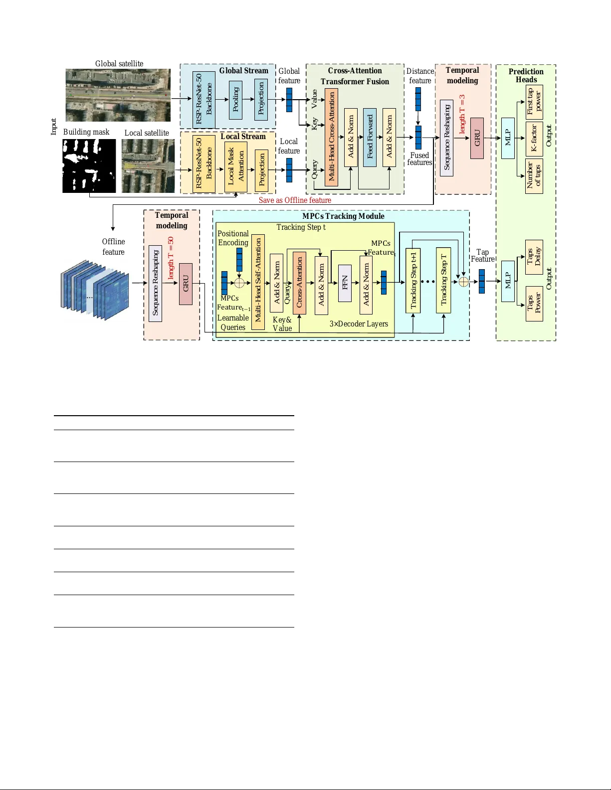
1 Deep Learning Based Site-Specific Channel Inference Using Satellite Images Junzhe Song, Ruisi He, Senior Member , IEEE, Mi Y ang, Member , IEEE, Zhengyu Zhang, Student Member , IEEE, Shuaiqi Gao, Bo Ai, F ellow , IEEE, Abstract —Site-specific channel inference plays a critical role in the design and evaluation of next-generation wireless com- munication systems by considering the surrounding pr opagation en vironment. Howev er , traditional methods are unscalable, while existing AI-based approaches using satellite image are confined to predicting large-scale fading parameters, lacking the capacity to reconstruct the complete channel impulse r esponse (CIR). T o address this limitation, we propose a deep learning-based site-specific channel inference framework using satellite images to predict structured T apped Delay Line (TDL) parameters. W e first establish a joint channel-satellite dataset based on measurements. Then, a novel deep learning network is developed to reconstruct the channel parameters. Specifically , a cross- attention-fused dual-branch pipeline extracts macroscopic and microscopic envir onmental features, while a recurrent tracking module captures the long-term dynamic evolution of multipath components. Experimental results demonstrate that the proposed method achieves high-quality reconstruction of the CIR in unseen scenarios, with a Power Delay Profile (PDP) A verage Cosine Similarity exceeding 0.96. This w ork provides a pathway toward site-specific channel inference for future dynamic wireless networks. Index T erms —Deep Learning, channel inference, channel mea- surements I . I N T RO D U C T I O N S ITE-SPECIFIC channel models characterize communica- tion links by considering the surrounding environmental geometry (e.g., buildings, vegetation, and moving objects) [1]. W ith the advancement of 5G and the evolution tow ards 6G, wireless scenarios are ev olving towards high mobility and dynamism (e.g., autonomous dri ving, v ehicular communi- cations, and unmanned aerial vehicle (U A V) networks) [2], [3]. The propagation characteristics in these scenarios are complex, and they are affected simultaneously by large-scale fading and rich multipath ef fects caused by dense scatterers. Therefore, obtaining high-fidelity Channel Impulse Response (CIR) data for these specific sites is fundamental to the design and performance ev aluation of next-generation communication systems [4], [5]. Existing standardized models such as 3GPP channel models [6], WINNER II [7], COST [8], [9], and the map-based METIS model [10] (e.g., the T apped Delay Line (TDL) models defined in 3GPP TR 38.901 [6], which parameterize the complex multipath propagation into a discrete set of signal taps J. Song, R. He, M. Y ang, Z. Zhang, S. Gao, and B. Ai are with the Schooof Electronics and Information Engineering, Beijing Jiaotong Univ ersity , Beijing 100044, China (email: 25115063@bjtu.edu.cn; ruisi.he@bjtu.edu.cn; myang@bjtu.edu.cn; 21111040@bjtu.edu.cn; 25110046@bjtu.edu.cn; boai@bitu.edu.cn) with specific delays and a verage powers) provide a structured format for extracting channel data. Despite their widespread use in system e valuations, they rely on generalized statistical distributions and fail to account for the unique en vironmental characteristics of specific sites. Manual calibration of these models for individual sites is inefficient and lacks generaliz- ability . Realistic site-specific channel modeling traditionally relies on Ray T racing (R T) [11] or empirical field measure- ments [12]–[20]. Although ray tracing is widely applied, it is computationally intensive and relies heavily on precise 3D en vironmental databases. In addition, simulations are less capable of capturing real-world complexity and dynamics than actual measurements. Howe ver , conducting extensi ve field measurements is expensi v e, laborious, and practically unscal- able in all deployment scenarios. Therefore, it is important to develop an efficient and generalizable approach for site- specific channel prediction. T o ov ercome the limitations of traditional modeling and extensi ve field measurements, Artificial Intelligence (AI)—particularly deep learning—has demonstrated excel- lence in handling non-linear , complex mapping relationships [21], [22]. In existing AI-driv en channel modeling research, en vironmental input features generally fall into two cate- gories: hand-crafted scalar inputs (e.g., transmitter-receiv er distance and regional building density) [23]–[27] and image- based inputs (e.g., satellite images, 2D en vironment models, and building masks) [28]–[34]. The former relies heavily on simplified statistical representations, making it difficult to accurately encapsulate abstract environmental contexts, such as the specific spatial distribution and geometric structures of physical scatterers. In contrast, for site-specific channel inference, satellite imagery emerges as an accessible and information-rich alternati ve. Specifically , satellite images can provide global views that cover the entire propagation path, which is crucial for capturing large-scale blockages. Further- more, they of fer high-resolution local views that capture the detailed en vironmental topology around the receiv er , which strictly dictates the behavior of small-scale multipath effects. Using the powerful spatial feature extraction capabilities of deep learning, it becomes feasible to directly extract the un- derlying ph ysical propagation mechanisms from these satellite images. Currently , models that use images as input focus primarily on large-scale channel parameters (e.g., path loss and signal quality parameters) [35]–[47]. Among these, advancing be- yond approaches that rely solely on fundamental Computer V ision (CV) pipelines, sev eral studies have incorporated phys- 2 ically interpretable feature designs to enhance the model’ s capacity to learn underlying propagation mechanisms. For example, W ang et al. developed a hybrid model-assisted framew ork that infuses domain-specific physical mechanisms directly into the data-dri ven architecture, enhancing the phys- ical consistency and generalization capabilities of the predic- tions in suburban scenarios [39]. Hayashi et al. incorporated deterministic path profiles along with 2D spatial information, representing the physical line-of-sight and terrain obstacles between transceiv ers to improv e the network’ s interpretation of terrain-induced propagation losses [47]. Zhu et al. utilized an adapti v e Meta Mask R-CNN model to identify and extract physical scatterer features from the input, bridging the gap between macroscopic environmental structures and path loss [36]. Despite these methodological advances in incorporating physical propagation mechanisms, a critical limitation persists in the current literature that these satellite-based approaches remain confined to the prediction of large-scale fading pa- rameters. Although some recent efforts have expanded their scope, for example, Li et al. predicted delay spread using Fresnel zone theory [48]. Howe ver , these outputs are restricted to statistical parameters. Consequently , these models lack the capacity to reconstruct the complete CIR, lea ving a g ap in fully characterizing the multipath behaviors required for modern wireless system e valuation. Bridging this gap in order to predict site-specific channel parameters from satellite image requires overcoming several challenges. First, in the spatial dimension, multipath propa- gation is physically af fected by both the macroscopic global en vironment and the microscopic local features. A single fea- ture extraction pipeline is fundamentally inadequate to balance both dimensions concurrently . Second, in the temporal dimen- sion, the dynamic birth-death processes and the ev olution of multipath components (MPCs) typically exhibit a pronounced long-term memory effect. Relying solely on static, single- frame satellite images makes it difficult to track these trajec- tories, as capturing their continuous ev olution fundamentally requires a broader temporal recepti ve field. Finally , re garding optimization, directly optimizing all network parameters in an end-to-end manner is challenging. Different channel parameter exhibit distinct physical sensitivities and ev olutionary time scales. Forcing a neural netw ork to learn these div erse physical characteristics simultaneously easily leads to sev ere gradient conflicts. T o address these challenges, we propose a deep learn- ing based site-specific channel inference frame work using satellite images. The parameters of the TDL model serve as the predictive targets, as their structured representation is compatible with neural network optimization paradigms. The framew ork integrates a dual-branch pipeline with a cross- attention fusion mechanism to capture ho w global macroscopic en vironments physically modulate local microscopic scatter- ing features. Furthermore, we introduce a specialized MPCs tracking module to model the dynamic temporal e volution of tap parameters, which is optimized via a decoupled multi- stage training strategy to prev ent gradient conflicts. The main contributions and innovations of this work are summarized as follows: • A dataset consisting of empirical channel measurements and satellite images is constructed. This dataset cov ers a variety of en vironments, including urban, suburban, and mixed scenarios. • A data preprocessing pipeline is dev eloped to extract TDL parameters from raw PDPs using dynamic thresholding and iterati ve peak extraction. Semantic se gmentation is applied to satellite images to generate b uilding masks. • A novel deep learning frame work, designed to fuse global and local en vironmental visual features, is introduced for the accurate prediction of TDL parameters. The remainder of this paper is org anized as follows: Sec- tion II outlines the proposed framework. Section III presents the channel measurement. Section IV details the data pre- processing. Section V details the architecture of the proposed model. Section VI ev aluates the performance of the model. Finally , Section VII concludes the paper . I I . C H A N N E L I N F E R E N C E F R A M E W O R K W e propose an AI-based Site-Specific Channel Inference using satellite images, with the ov erall framework illustrated in Fig. 1. The proposed method uses both channel data and satellite data to train a model capable of predicting CIR. Channel data can typically be obtained through Ray-T racing simulations or real-world measurements. Compared to Ray- T racing, measurement-based data of fer greater authenticity and representativ eness in capturing en vironmental complexity and dynamic variations, making them more suitable for e v aluating the generalization capability of the model. W e built a measure- ment platform capable of data acquisition.The receiv er antenna acquires the raw in-phase and quadrature (IQ) signals, which are calibrated and transformed to obtain the CIR and PDP . Meanwhile, the GPS data collected by the rubidium clock are used to extract the corresponding site-specific satellite image. During the data preprocessing stage, the TDL parameters are chosen to abstract the ra w channel information, as their highly structured format is compatible with neural network training. The raw PDP under gos a refinement comprising three sequential operations: signal filtering to denoise, multipath extraction to identify dominant propagation paths, and param- eter calculation to quantify the statistical channel behavior . Specifically , the TDL parameters comprise the large-scale fading parameter P (characterized by the first tap power), the K-factor K , the total number of taps N , the tap Normalized delays τ = { τ 1 , τ 2 , · · · τ N } , and their corresponding tap powers p = { p 1 , p 2 , · · · p N } . It is worth noting that as this work is conducted under LOS scenarios, the K-factor K practically corresponds to the first tap, which follows a Rician distribution. TDL parameters can be expressed as: Θ = {P , K, N , τ , p } (1) The collected satellite imagery is preprocessed through image cropping , annotation, and mask generation operations. These image processing steps establish a satellite dataset comprising global satellite views that cov er the entire propaga- tion path, local satellite vie ws capturing en vironmental details 3 M u l t i - S t a g e C h a n n e l - to - R e c o n st r u c t i o n ( M S C R ) N e t w o r k D a t a P r e p r o c e ssi n g S a m p l i n g P C A C r o p p i n g S t e p 1 : S t e p 2 : S t e p 3 : S A G E D e n o i si n g F i l t e r i n g S t e p 1 : S t e p 2 : S t e p 3 : H H H H H H S t e p 4 : M a t c h i n g Li d a r a n d c h a n n e l p a r a me t e r d a t a S t e p 5 : M a k i n g sce n e l a b e l D a t a se t ... ... D a t a D r i v e n C h a n n e l C h a r a c t e r i st i c En c o d e r S c e n e R e c o n st r u c t i o n D e c o d e r S u p e r v i si o n I n p u t s Li d a r Po i n t c l o u d C h a n n e l D a t a R e c o n st r u c t e d sce n e De lay De lay AOA AOA E OA E OA T r a ns mit ter Ante n na R e c e iver Ante n na I Q S ign a l s C I R & P D P S i gna l F il ter ing M ult i pa th E xt r a c ti on P a r a mete r C a lcula ti on Step1 : Step2 : Step3 : R ubid ium C locks GP S Da ta S i te - s pe c if ic S a telli te S u r r o unding E nvir onment M a s k Anno tation C r op ping Step1 : Step2 : Step3 : Dat a A c q u i s it ion Dat a P r e p r oc e s s in g Tr a n smi t t e r A n t e n n a R e c e i v e r A n t e n n a IQ S i g n a l s C I R & P D P S i g n a l F i l t e r i n g M u l t i p a t h E x t r a c t i o n P a r a met e r C a l c u l a t i o n S t e p 1 : S t e p 2 : S t e p 3 : R u b i d i u m C l o c k s G P S D a t a Si t e - sp e c i f i c S a t e l l i t e Su r r o u n d i n g En v i r o n me n t M a sk A n n o t a t i o n C r o p p i n g S t e p 1 : S t e p 2 : S t e p 3 : D a t a a c q u i si t i o n D a t a P r e p r o c e ssi n g Glob a l S a telli te M a sk A n n o t a t i o n C r o p p i n g L oc a l S a telli te B uil d ing M a s k F i r s t T a p powe r K - f a c to r Num be r of T a p s T a ps De lay T a ps P o we r Dat as e t C on s t r u c t ion T DL Da tas e t S a t e l li te Da tas e t N e t w o r k C I R AI - ba s e d S it e - S p e c i f ic C ha nne l I nf e r e nc e Fig. 1. An o vervie w of the proposed method framework. strictly around the RX, and binary building masks representing en vironmental scatterers and blockages. Subsequently , the processed satellite image S and the set of TDL parameters Θ are paired sample by sample to construct the dataset based on timestamp and spatial location to ensure en vironmental consistency across the training data. Gi ven that both the channel measurements and the GPS data are time-stamped by the same rubidium clock, their alignment is inherently achiev ed without manual ef fort. The model is trained on the constructed dataset to learn a mapping from the satellite image to the TDL parameters: ˆ Θ = f ( S ) (2) where S denotes the input set of satellite image, ˆ Θ is the predicted TDL parameters, and f represents the proposed model, which will be elaborated in Section V . I I I . C H A N N E L M E A S U R E M E N T S In this section, we describe the previous measurement campaigns conducted to validate the proposed reconstruction framew ork. These measurements provide the foundation for establishing the joint channel-satellite dataset, ensuring that the subsequent deep learning model is trained on physically accurate propagation characteristics. A. Measurement Setup W e conducted measurement campaigns using the equipment shown in Fig. 2. The measurement system consists of trans- TX V ehic le RX Veh ic le Block diagram of the measu rement sy stem TX An te nn a RX A ntenn a Ar ray GN SS Antenn a Po wer Am plifie Vector Sign al Tran sm it te r Rub idium cl ock Mea su rem ent veh ic le s and antenn as TX veh ic le equ ipm ents RX an te nn a rad ia ti on patte rn ɵ= 90 ° Φ = 0 ° ɵ= 0 ° Φ = 90 ° ɵ= 0 ° Φ = 0 ° Measur eme n t R out e Me asur em ent Rou te Me asur em ent area Fig. 2. Measurement system architecture and key equipment. T ABLE I C O NFI G U R A TI O N S O F M E A S UR E M E NT S Y ST E M Parameters V alue Center frequency 5.8 GHz Bandwidth 30 MHz T ransmit po wer 45 dBm Sounding signal Multi-carrier signal Number of frequency points 1024 T ransmitter antenna Omnidirectional antenna Receiv er antenna 4 × 8 planar array mitting (Tx) and receiving (Rx) subsystems integrated into vehicles, with the core components being a vector signal gen- erator (VSG) and a vector signal analyzer (VSA). Specifically , the VSG and VSA are NI PXIe-5673 and NI PXIe-5663, respectiv ely . The sounding signal is a broadband multi-carrier signal with 513 subcarriers o ver a bandwidth of 30 MHz. The TX antenna is an omnidirectional single element an- tenna, while the RX antenna is a 4×8 array . Both TX and RX antennas are mounted on vehicle roofs at a height of approximately 1.8 m. The Z axis of the RX antenna array is oriented opposite to the v ehicle’ s forward direction. Each element of the RX antenna array is connected to a vector signal analyzer through an electronic switch, because the TDL dataset in this w ork does not contain angular parameters, only the data collected from a single antenna element within the RX array was actually used. For precise time synchronization, two GPS-referenced rubidium clocks disciplined by Global Navigation Satellite System (GNSS) signals are employed. These clocks also provide real-time longitude and latitude coordinates, enabling accurate positioning of both Tx and Rx and site-specific satellite image acquisition. T able I summarizes the detailed configurations of the mea- surement system. The measurement bandwidth is 30 MHz, resulting in a delay resolution of 33.3 ns. For sub-6 GHz ve- hicular communications, the available bandwidth is generally 20–30 MHz, which is similar to the measurement configuration in this article. The acquisition rate of channel snapshots is 45 snapshots/s when measured. B. Measurement Campaign As illustrated in Fig. 3, measurement campaigns were conducted across di verse en vironments to establish a robust and representative dataset. The measurement locations span two cities. Specifically , the aerial maps in Fig. 3(a)-(c) present 4 T est r o u t e TX V alid atio n r o u te T r ain r o u t e T est r o u t e TX V alid atio n r o u te T r ain r o u t e T est 1 T est 1 T est 2 T est 2 T est 3 T est 3 ( a) ( a) ( b ) ( b ) ( c) ( c) ( d ) ( d ) Fig. 3. Measurement Scenarios. the various measurement sites deployed in Beijing, china, while Fig. 3(d) presents the measurement area in Chang- sha, china. Furthermore, the measurement sites cov er diverse en vironmental complexities, spanning urban, suburban, and mixed propagation scenarios. As shown in Fig. 3(a) and 3(b), the typical urban areas are characterized by dense buildings, complex intersections, and rich scatterers. In contrast, Fig. 3(c) illustrates a typical suburban en vironment with a more open layout, sparse structures, di verse ve getation, and unique spatial geometries. Finally , Fig. 3(d) presents a mix ed scenario containing both buildings and vegetation. This measurement campaign ensures the richness and div ersity of the collected dataset. I V . D A TA P R E - P RO C E S S I N G In this section, we presents the dataset preprocessing and construction workflo w . First, we detail the extraction of re- liable TDL parameters from the raw PDPs via dynamic thresholding and iterativ e peak extraction techniques. Next, we describe the rigorous spatial alignment, cropping, and semantic segmentation of the satellite images. Finally , the dataset splitting methodology is summarized. A. TDL P arameters Calculation Fig. 4 details the construction procedure of the TDL pa- rameter dataset. T o suppress random fast fading and system noise for reliable small-scale multipath extraction, the raw PDPs undergo sliding-windo w statistical averaging in the time domain to yield the APDP . Next, an adaptive dynamic thresholding method is employed for denoising. Specifically , valid APDP samples above the absolute noise floor (-160 dB) are isolated and sorted by po wer . The mean of the bottom 20% samples is calculated as the real-time noise floor estimate for the given window . By adding an empirical 11 dB noise mar gin to this estimate, a dynamic truncation threshold is dynamically generated for each snapshot. Components falling belo w this threshold are classified as background noise and truncated to -200 dB. This procedure ensures that the TDL taps deriv ed Algorithm 1 Iterative Peak Search for TDL T ap Extraction Require: A veraged PDP P av g , Max taps limit N max , Dy- namic range threshold D th , Minimum separation δ Ensure: Set of e xtracted taps T = { ( τ i , P i ) } 1: Initialize tap set T ← ∅ 2: Initialize residue PDP P res ← P av g 3: Calculate global maximum P g lobal ← max( P res ) 4: Set cut-off threshold P limit ← P g lobal − D th 5: 0) Pr e-compute Local P eaks Mask: ▷ Prev ent extracting side-lobes 6: Generate binary mask M local of same length as P res , where: 7: M local [ τ ] ← 1 if P res [ τ ] > max( P res [ τ − 1] , P res [ τ + 1]) else 0 8: for k ← 1 to N max do 9: 1) F ind Global Maximum in Local P eaks: 10: Apply mask to search space: P search ← P res ⊙ M local ▷ Element-wise product 11: Find peak index τ k ← arg max τ ( P search ) 12: Get peak po wer P k ← P res ( τ k ) 13: 2) Dynamic Range Chec k: 14: if P k < P limit or P k == 0 then 15: break ▷ Remaining peaks are considered noise or in v alid 16: end if 17: 3) Recor d T ap: 18: T ← T ∪ { ( τ k , P k ) } 19: 4) Spatial Masking: 20: Determine windo w start n start ← max(1 , τ k − δ ) 21: Determine window end n end ← min( length ( P res ) , τ k + δ ) 22: P res [ n start : n end ] ← 0 ▷ Zero out neighbor re gion 23: M local [ n start : n end ] ← 0 ▷ Update mask to a void duplicate extraction 24: end for 25: return T from the processed APDP are strictly composed of multipath components. Subsequently , for each snapshot, an iterativ e peak extraction algorithm is e xecuted, as outlined in Algorithm 1. Specifically , all local po wer maxima in the APDP are e xtracted as candidate taps. The algorithm then enters an iterati ve loop to find the global maximum peak in the residual signal. T o accommodate the dynamic SNR of different snapshots, a relati ve truncation threshold is set 50 dB below the current highest peak; peaks below this le v el are treated as noise, terminating the loop. Once a valid tap is extracted, the signal within a neighborhood of 3 samples on either side of its center is forced to zero. This critical step prev ents the energy leakage induced by channel dispersion from being falsely detected as separate multipath arriv als, ensuring that the extracted taps remain physically independent. Once the delay positions of all multipath taps are deter- mined, a local delay window is defined for each tap, starting from the current tap and terminating at the arri v al time of the subsequent tap. the tap power is computed by integrating the 5 F ir st T a p p o w e r R aw P D P P r ocessed A P D P … A P D P S napsh ot … TD L D at aset • S ta tistica l A ve r a g ing • Den o isi n g • S n a p sh o t E x tr a ctio n • I te r a tive P e a k E x tr a ctio n • M P C Cl u ste r ing • T a p P a r a m e te r Calcu lat ion Del a y [ n s] Del a y [ n s] P o w e r [d B m ] I n p u t G l o b a l S t r e a m P o o l i n g P r o j e c t i o n R S P - R e s N e t - 50 B a c k b o n e L o c a l S t r e a m L o c a l M a s k A t t e n t i o n R S P - R e s N e t - 50 B a c k b o n e P r o j e c t i o n G l o b a l s a t e l l i t e L o c a l s a t e l l i t e B u i l d i n g m a s k C r o s s - A t t e n t i o n T r a n s f o r m e r F u s i o n G l o b a l f e a t u r e L o c a l f e a t u r e M u l t i - H e a d C r o s s - A t t e n t i o n Q u e r y K e y V a l u e A d d & N o r m F e e d F o r w a r d A d d & N o r m S a v e a s O f f l i n e f e a t u r e D i s t a n c e f e a t u r e F u s e d f e a t u r e s S e q u e n c e R e s h a p i n g l e n g t h T = 3 G R U T e m p o r a l m o d e l i n g S e q u e n c e R e s h a p i n g l e n g t h T = 5 0 G R U T e m p o r a l m o d e l i n g M P C s T r a c k i n g M o d u l e F F N C r o s s - A t t e n t i o n M u l t i - H e a d S e l f - A t t e n t i o n T r a c k i n g S t e p t T r a c k i n g S t e p t + 1 F i r s t t a p p o w e r A d d & N o r m A d d & N o r m A d d & N o r m MPC s F eatu r e t T r a c k i n g S t e p T M L P P r e d i c t i o n H e a d s K - f a c t o r N u m b e r o f t a p s O u t p u t T a p s D e l a y M L P T a p s P o w e r O u t p u t O f f l i n e f e a t u r e MPC s F eatu r e t − 1 P o s i t i o n a l E n c o d i n g T a p F e a t u r e 3× D e c o d e r L a y e r s L e a r n a b l e Q u e r i e s K e y & V a l u e Q u e r y K - fa cto r Num b e r o f ta p s T a p s Dela y T a p s P o w e r Fig. 4. Procedure of construct TDL parameters dataset. TX RX B u i l d i n g m a s k G l o b a l s a t e l l i t e L o c a l s a t e l l i t e S i g n a l R a d i a t i o n D i r e c t i o n S e g F o r m e r ( H i e r a r c h i c a l T r a n s f o r m e r E n c o d e r ) P a t c h E m b e d A l l - M L P D e c o d e r L i g h t w e i g h t O v e r l a p p e d P a t c h M e r g i n g M i x - F F N w i t h P o s i t i o n a l E n c o d i n g S e l f - A t t e n t i o n 𝐻 4 × 𝑊 4 × 𝐶 1 𝐻 32 × 𝑊 32 × 𝐶 4 𝐻 4 × 𝑊 4 × 𝐶 1 𝐻 8 × 𝑊 8 × 𝐶 2 𝐻 16 × 𝑊 16 × 𝐶 3 𝐻 32 × 𝑊 32 × 𝐶 4 𝐻 8 × 𝑊 8 × 𝐶 2 𝐻 16 × 𝑊 16 × 𝐶 3 Fig. 5. Procedure of construct satellite dataset. energy over this interv al. After calculating the power P ′ and the delay of the first tap, a normalization process is applied to all taps to obtain the normalized delay array τ and the power array p . Furthermore, the absolute maximum power of the first tap on the APDP is treated as the pure LOS path power p LOS . The NLOS power p N LO S , contributed by micro-scatterers arriving closely behind the main path, is then obtained by subtracting p LOS from the total inte grated po wer of the first tap’ s local window . Finally , the Rician K-factor K for the snapshot is calculated as K = p LOS − p N LO S . B. Satellite Image Pr e-pr ocessing Fig. 5 illustrates the procedure for constructing the satellite dataset. First, to capture the global large-scale blockages and environmental features between the Tx and the Rx, the physical distance and azimuth angle of the propagation link are computed based on their respective coordinates. An en- compassing Re gion of Interest (ROI) is then cropped from the original image. Subsequently , a rotation alignment operation is performed to map all Tx-Rx links to a horizontal orientation. Furthermore, to prev ent dimensional distortion caused by excessi vely short propagation distances, the cropping width is dynamically set to the maximum of 1.1 times the physical distance and 256 m, paired with a fixed street-lev el height of 128 m. The resulting image is then resized to 512 × 256 pixels. Additionally , Tx/Rx node markers and the Line-of- Sight (LOS) trajectory are annotated onto the image to enhance the neural network’ s perception of the link topology . The local scattering en vironment surrounding the Rx plays a critical role in determining multipath ef fects. After applying the same rotation alignment, a square physical receptiv e field of 256 m × 256 m, centered at the Rx coordinates, is cropped. This re gion is then resized to a standard of 224 × 224 pixels, matching the input requirements of popular vision backbones (e.g., ResNet or V iT). Furthermore, the Rx location and the approximate direction of signal arriv al are annotated onto the image. Meanwhile, to assist the model in learning the critical physi- cal propagation mechanism of b uilding blockages, an adv anced semantic se gmentation model based on the T ransformer archi- tecture (Segformer-B1) is introduced [49]. Giv en the relati vely low resolution of the local micro-views (224 × 224), an image interpolation enhancement strategy is employed during the inference stage. Specifically , the input images are upsampled to 1024 × 1024 to fully acti vate the Segformer’ s pre-trained weights deriv ed from high-resolution remote sensing datasets, thereby precisely capturing the edges of building footprints. After the model output is restored to its original size using bilinear interpolation, the ’building’ cate gory is extracted to generate a binary semantic mask. This mask serves as an additional modal input, guiding the network to learn pure physical scattering mechanisms. C. Dataset Construction The processed satellite images and the TDL parameter sets are paired on a sample-by-sample basis according to their specific timestamps and spatial locations, thereby ensuring the en vironmental consistency of the dataset. Gi ven the high similarity in spatial environmental features among adjacent samples along the same route, a route-based dataset splitting strategy is adopted instead of the con ventional random splitting approach. This design prev ents potential spatial data leakage during the model training phase. The partitioning of the dataset is illustrated in Fig. 3, comprising a total of 16,800 samples. 6 I n p u t G lo ba l St re a m Po o lin g Pro jectio n R SP - R esNet - 50 B ac k b o n e L o ca l St re a m L o ca l M ask Atten tio n R SP - R esNet - 50 B ac k b o n e Pro jectio n Glo b al s at ellite L o ca l s at ellite B u il d in g m as k Cro s s - At t ent io n T ra n s f o rm er F us io n Glo b al f ea tu r e L o ca l f ea tu r e Mu lti - Hea d C r o s s - Atten tio n Qu er y Key Valu e Ad d & No r m Feed Fo r war d Ad d & No r m Sav e as Of f lin e f ea tu r e Dis tan ce f ea tu r e Fu s ed f ea tu r es Seq u en ce R esh ap i n g len g t h T = 3 GR U T empo ra l mo del ing Seq u en ce R esh ap i n g len g t h T = 5 0 GR U T empo ra l mo del ing M P Cs T ra ck ing M o du le FF N C r o s s - Atten tio n Mu lti - Hea d Self - Atten tio n T r ac k in g Step t T r ac k in g Step t+1 Firs t ta p p o w er Ad d & No r m Ad d & No r m Ad d & No r m MPC s F eatu r e t T r ac k in g Step T MLP P re dict io n H ea d s K - f acto r Nu m b er o f tap s Ou tp u t T ap s Dela y MLP T ap s Po wer Ou tp u t Of f lin e f ea tu r e MPC s F eatu r e t − 1 Po s i tio n al E n co d in g T ap Featu r e 3× Dec o d er L ay er s L ea r n ab le Qu er ies Key & Valu e Qu er y Fig. 6. The proposed model. T ABLE II D E T A IL E D A R C H I TE C T U RE O F T H E P RO P O S ED M O DE L Network Layer Output Description Input G/L Satellite ( B × T , 3, H , W ) / Mask ( B × T , 1, H , W ) / Dist. Feat. ( B × T , 1) / Global ResNet-50 ( B × T , 2048, h , w ) / Pooling ( B × T , 2048) GAP Projection ( B × T , 512) 2048 → 512 Local ResNet-50 ( B × T , 2048, h , w ) / Mask Attn. ( B × T , 2048) GAP Projection ( B × T , 512) 2048 → 512 Cross-Attn. MH Attn. ( B × T , 512) L:2, H:4 Concat. ( B × T , 513) 512 + 1 → 513 T emporal Reshape ( B , T , 513) / GR U ( B , T , 513) L:1, Hid:513 T racking Pos. Enc. ( B , T , N , 513) / Decoder ( B , T , N , 513) L:3, H:9 Pred. Heads MLP ( P ) ( B , T , 1) 513 → 128 → 64 → 1 MLP ( K / N ) ( B , T , 1) 513 → 128 → 1 MLP ( τ / p ) ( B , T , N ) 513 → 1 Note: G/L: Global/Local, Attn.: Attention, GAP: Global A verage Pooling, L: Layers, H: Heads, Hid: Hidden size, P : First tap power , K : K-factor , N : Number of taps, τ : T aps Delay , p : T aps Power . V . M O D E L D E S I G N In this section, we detail the proposed model framew ork for inference of site-specific channel parameters. The model integrates a Cross-Attention Transformer Fusion module that dynamically modulates local spatial features using global en vironmental constraints. The model incorporates specialized temporal prediction modules. These include a short-sequence temporal modeling component and a long-sequence MPCs tracking module designed to rigorously capture the dynamic birth-death processes of tap parameters. W e subsequently outline a decoupled, multi-stage training strate gy . A. Model Structur e The proposed model aims to process satellite images, learn macro- and micro-propagation mechanisms in wireless chan- nels, and extract spatiotemporal features for predicting TDL parameters, as shown in Fig. 6. The framew ork employs a dual-branch feature extraction pipeline. T o capture large-scale fading effects, the Global Stream processes global satellite images using a Remote Sensing Pretraining-ResNet-50 (RSP- ResNet-50) backbone to extract the global features of the LOS link. Meanwhile, since small-scale fading is primarily dependent on the en vironment surrounding the RX, the Local Stream is tasked with extracting local features. Moreover , a Local Mask Attention mechanism is introduced to fuse the building mask with these local features. This design compels the network to focus on significant buildings responsible for signal reflection and dif fraction, suppressing interference from irrelev ant features and enhancing the physical rationality of the local feature extraction. Multipath propagation is physically constrained by the global en vironmental, for instance, dense urban buildings in urban areas trigger multiple reflection and diffraction, multi- path ef fects in suburban areas are relativ ely weak. T o capture 7 T est 1 P ro po s ed M o d el RM SE P a t h L o s s : 5 . 6 2 d B RM SE Dela y Sp re a d : 9 7 . 4 5 ns RM SE K - F a ct o r: 2 . 4 6 d B Av g C o s ine Sim ila rit y : 0 . 9 6 4 3 P ro po s ed M o d el G ro u nd T rut h T est 1 T est 2 P ro po s ed M o d el RM SE P a t h L o s s : 4 . 7 1 d B RM SE Dela y Sp re a d : 4 4 . 4 8 ns RM SE K - F a ct o r: 2 . 8 5 d B Av g C o s ine Sim ila rit y : 0 . 9 7 3 5 6 0 0 0 T est 2 T est 3 T est 3 P ro po s ed M o d el RM SE P a t h L o s s : 5 . 2 1 d B RM SE Dela y Sp re a d : 1 0 5 . 5 3 n s RM SE K - F a ct o r: 2 . 0 1 d B Av g C o s ine Sim ila rit y : 0 . 9 6 1 6 Gro u n d Tru th P re d ic t io n Gro u n d Tru th P re d ic t io n Gro u n d Tru th P re d ic t io n Gro u n d Tru th P re d ic t io n Gro u n d Tru th P re d ic t io n Gro u n d Tru th P re d ic t io n T est 1 T est 2 T est 3 Gr o u n d T r u th Pre d ictio n Gr o u n d T r u th Pre d ictio n Sn ap s h o t I n d e x Path L o s s [ d B ] T est 2 US ARP [ 4 5 ] RM SE P a t h L o s s : 7 . 2 5 d B RM SE Dela y Sp re a d : 1 2 7 . 6 0 n s RM SE K - F a ct o r: 3 . 0 7 d B Av g C o s ine Sim ila rit y : 0 . 9 6 9 5 T est 3 US ARP [ 4 5 ] RM SE P a t h L o s s : 7 . 0 0 d B RM SE Dela y Sp re a d : 1 5 9 . 5 4 n s RM SE K - F a ct o r: 1 . 5 0 d B Av g C o s ine Sim ila rit y : 0 . 9 4 4 3 T est 1 US ARP [ 4 5 ] RM SE P a t h L o s s : 7 . 7 1 d B RM SE Dela y Sp re a d : 2 2 7 . 8 8 n s RM SE K - F a ct o r: 2 . 7 6 d B Av g C o s ine Sim ila rit y : 0 . 9 6 7 1 T est 1 w/o Cro s s - At t ent io n RM SE P a t h L o s s : 5 . 3 9 d B RM SE Dela y Sp re a d : 2 0 6 . 8 6 n s RM SE K - F a ct o r: 3 . 1 1 d B Av g C o s ine Sim ila rit y : 0 . 9 6 2 9 T est 2 w/o Cro s s - At t ent io n RM SE P a t h L o s s : 5 . 0 3 d B RM SE Dela y Sp re a d : 2 8 3 . 8 2 n s RM SE K - F a ct o r: 3 . 3 6 d B Av g C o s ine Sim ila rit y : 0 . 9 5 9 2 T est 3 w/o Cro s s - At t ent io n RM SE P a t h L o s s : 5 . 5 3 d B RM SE Dela y Sp re a d : 1 8 9 . 4 7 n s RM SE K - F a ct o r: 1 . 6 8 d B Av g C o s ine Sim ila rit y : 0 . 9 2 5 8 T est 1 w/o G RU & T ra ck ing RM SE P a t h L o s s : 1 0 . 8 6 dB RM SE Dela y Sp re a d : 1 2 2 . 2 9 n s RM SE K - F a ct o r: 2 . 1 1 d B Av g C o s ine Sim ila rit y : 0 . 8 9 4 2 T est 2 w/o G RU & T ra ck ing RM SE P a t h L o s s : 1 1 . 0 3 dB RM SE Dela y Sp re a d : 9 8 . 4 3 ns RM SE K - F a ct o r: 4 . 0 8 d B Av g C o s ine Sim ila rit y : 0 . 9 2 2 3 T est 3 w/o G RU & T ra ck ing RM SE P a t h L o s s : 8 . 7 7 d B RM SE Dela y Sp re a d : 2 0 3 . 1 6 n s RM SE K - F a ct o r: 1 . 6 6 d B Av g C o s ine Sim ila rit y : 0 . 9 3 6 1 US ARP [ 4 3 ] w/o G RU & T ra ck ing w/o Cro s s - At t ent io n Fig. 7. PDP comparisons. this modulating ef fect of the macroscopic en vironment on mi- croscopic multipath phenomena, the model employs a Cross- Attention T ransformer Fusion module to perform cross-scale feature interaction. Specifically , the local features representing the microscopic environment serve as the Query vectors, while the global features denoting the macroscopic en vironment act as the K ey and V alue vectors. This fusion strategy enables the global features to dynamically modulate the local ones. Acting like a filter , it empowers the model to capture which specific local features are critical to the multipath effects under the current macroscopic scenario. Giv en the gradual ev olution of the physical en vironment along the continuous trajectory of the RX, the large-scale fading and multipath effects of the channel typically exhibit high spatial consistency and temporal correlation over short periods. T o prev ent observation errors or local visual abrup- tions in single-frame static satellite images from causing non- physical drastic fluctuations in the predicted parameters, the fused features are concatenated with the Tx-Rx distance and subsequently input into a short-sequence temporal modeling module. This module, employing a Gated Recurrent Unit (GR U) with a time step of T s = 3 , is designed to capture the short-term spatial smoothness between adjacent snapshots along each route, thereby regularizing the feature representa- tions. Ultimately , the output of this module is passed through a Multi-Layer Perceptron (MLP) prediction head to regress the preliminary TDL parameters, including the first tap po wer , K- factor , and the number of taps. An independent MPC T racking Module is designed to pre- dict the complex, dynamically evolving tap delay and power arrays. The birth-death processes and e v olution of MPCs typi- cally exhibit a pronounced long-term memory effect. a broader temporal recepti ve field is required to capture their ev olution. T o achiev e this while avoiding computational ov erhead and GPU memory bottlenecks, offline features are introduced. Specifically , the frame-lev el spatial fusion features output by the Cross-Attention T ransformer Fusion module are cached offline. Before the T racking Module, these offline features are directly retrie ved and reorganized into long sequences ( T l = 50 ), and passed to a separate GR U for long-term temporal encoding. Follo wing this, a recurrent Transformer decoder architecture is employed. At each tracking step t , the prior multipath state (MPCs Feature t − 1 ) and a learnable query positional encoding compute multi-head self-attention, 8 RM SE P a t h L o s s : 5 . 6 2 d B RM SE Dela y Sp re a d : 9 7 . 4 5 ns RM SE K - F a ct o r: 2 . 4 6 d B Av g C o s in e S im il a rity : 0 . 9 6 4 3 P re dict io n G ro u nd T rut h T est 1 RM SE P a t h L o s s : 4 . 7 1 d B RM SE Dela y Sp re a d : 4 4 . 4 8 ns RM SE K - F a ct o r: 2 . 8 5 d B Av g C o s ine Sim ila rit y : 0 . 9 7 3 5 6 0 0 0 T est 2 T est 3 Sa mp les: 2 1 6 RM SE P a t h L o s s : 5 . 2 1 d B RM SE Dela y Sp re a d : 1 0 5 . 5 3 n s RM SE K - F a ct o r: 2 . 0 1 d B Av g C o s ine Sim ila rit y : 0 . 9 6 1 6 G ro u n d T ru th P re d ic t io n G ro u n d T ru th P re d ic t io n Gro u n d Tru th P re d ic t io n Gro u n d Tru th P re d ic t io n Gro u n d Tru th P re d ic t io n Gro u n d Tru th P re d ic t io n T est 1 T est 2 T est 3 Fig. 8. CDF comparison between the proposed model and measured data. followed by cross-attention with the temporally encoded of- fline features. This iterati ve attention-based tracking models the temporal coherence and trajectories of MPCs as the RX mov es. Finally , the aggregated tap features are routed to specific MLP heads to predict tap delays and powers. The detailed architecture of the proposed model is sho wn in T able II. B. Loss Functions and T r aining Strate gies In the proposed model, directly optimizing all parameters in an end-to-end manner is a highly challenging task. The TDL parameters exhibit distinct physical sensitivities and ev olution- ary time scales. T o prevent gradient conflicts and ensure that each module learns its designated physical mechanism, we adopt a decoupled, multi-stage training strategy . The netw ork is trained progressi vely , with each stage freezing specific upstream modules to stabilize the feature representations. 1) T raining Stage I: Lar ge-scale fading P : : In the first stage, the network focuses on extracting the Global feature. The Global Stream, the First T ap Power prediction head, and the GRU are acti vated, while all other modules are frozen. Since the first tap power represents the large-scale fading which v aries smoothly along the moving trajectory , we formulate the loss function as a combination of Mean Squared Error (MSE) and a temporal consistenc y regularization term: L 1 = 1 B · T s B X b =1 T s X t =1    ˆ P b,t − P b,t    2 + λ 1 L temp ( ˆ P ) (3) where B is the batch size, T s = 3 is the short sequence length used in this stage, and ˆ P b,t and P b,t are the predicted and ground-truth normalized first tap powers, respectively . The temporal consistency loss L temp penalizes abrupt, non- physical fluctuations between adjacent snapshots to mitigate observation noise from static satellite images: L temp ( ˆ P ) = 1 B ( T s − 1) B X b =1 T s X t =2    ˆ P b,t − ˆ P b,t − 1    2 (4) where λ 1 is empirically set to 0.1. 2) T raining Sta ge II: Statistical Channel Attributes ( K and N ): The second stage aims to parameterize the statistical properties of the local scattering en vironment, specifically the Ricean K-factor and the total number of MPC taps. The Global Stream is frozen to serve as a stable macroscopic context provider , while the Local Stream, the Cross-Attention Fusion module, and their corresponding prediction heads are optimized. The loss function for this stage is defined as: L 2 = MSE( ˆ K , K ) + MSE( ˆ N , N ) + λ 1 L temp ( ˆ K ) (5) RM SE P a t h L o s s : 5 . 6 2 d B RM SE Dela y Sp re a d : 9 7 . 4 5 ns RM SE K - F a ct o r: 2 . 4 6 d B Av g C o s in e S im il a rity : 0 . 9 6 4 3 P re dict io n G ro u nd T rut h T est 1 RM SE P a t h L o s s : 4 . 7 1 d B RM SE Dela y Sp re a d : 4 4 . 4 8 ns RM SE K - F a ct o r: 2 . 8 5 d B Av g C o s ine Sim ila rit y : 0 . 9 7 3 5 6 0 0 0 T est 2 T est 3 Sa mp les: 2 1 6 RM SE P a t h L o s s : 5 . 2 1 d B RM SE Dela y Sp re a d : 1 0 5 . 5 3 n s RM SE K - F a ct o r: 2 . 0 1 d B Av g C o s ine Sim ila rit y : 0 . 9 6 1 6 G ro u n d T ru th P re d ic t io n G ro u n d T ru th P re d ic t io n Gro u n d Tru th P re d ic t io n Gro u n d Tru th P re d ic t io n Gro u n d Tru th P re d ic t io n Gro u n d Tru th P re d ic t io n T est 1 T est 2 T est 3 Gr o u n d T r u th Pre d ictio n Gr o u n d T r u th Pre d ictio n Sn ap s h o t I n d e x Path L o s s [ d B ] Fig. 9. Path loss comparison between the proposed model and measured data. where ˆ K and ˆ N denote the predicted K-factor and the number of taps, respectiv ely . By isolating this training stage, the Local Stream is forced to learn ho w the local semantic masks (e.g., buildings) interact with the global path constraints to determine the multipath richness, pre venting the network from prematurely ov erfitting to the e xact delays of indi vidual MPCs. 3) T raining Stage III: MPCs T racking ( τ and p ): The final stage reconstructs the fine-grained TDL parameters by predicting the specific delay and relativ e power of each tap. T racking the birth, e volution, and death of indi vidual multipath clusters requires a significantly lar ger temporal receptive field. W e extract and freeze the output representations from the previously trained spatial fusion modules and sav e them as offline features. This allo ws us to drastically expand the sequence length to T l = 50 for the MPC T racking Module without repeatedly ex ecuting the hea vy CNN backbones. Since the extracted MPCs are essentially an unordered set of points, standard point-to-point loss functions cannot be directly applied. W e model the MPCs prediction as a bipartite matching problem and employ a matching loss coupled with a physical repulsion constraint: L 3 = L match + α L rep (6) The matching loss L match utilizes the Hungarian algorithm [50] to find the optimal assignment σ between the predicted tap set ˆ Y = { ˆ τ , ˆ p } and the ground-truth tap set Y { τ , p } : L match = 1 B · T l X b,t 1 | V | X j ∈ V | ˆ y σ ( j ) − y j | 2 (7) where y j = [ w d · τ j , p j ] represents the scaled delay and po wer of the j -th ground-truth tap, w d is a weighting factor to balance the scale difference between the delay and power domains, and V is the set of valid (non-padded) ground-truth taps. T o prev ent the T ransformer decoder from collapsing multiple predicted queries into the same dominant multipath cluster, we introduce a repulsion loss L rep to enforce a minimum physical separation threshold d min between any two predicted delays: L rep = 1 B · T l · N ( N − 1) X b,t X i  = j max(0 , d min − | ˆ τ i − ˆ τ j | ) (8) 9 T ABLE III P E RF O R M AN C E C O M P A R IS O N OF D I FFE R E N T M E TH O D S I N T ES T S T est Route Method RMSE Path Loss [dB] RMSE Delay Spread [ns] RMSE K-Factor [dB] PDP A verage Cosine Similarity T est 1 Proposed Model 5.62 97.45 2.46 0.9643 USARP [43] 7.71 227.88 3.76 0.9071 w/o Cross-Attention 8.39 206.86 3.11 0.9229 w/o GRU & T racking 10.86 122.29 2.91 0.8942 T est 2 Proposed Model 4.71 44.48 2.85 0.9735 USARP [43] 7.25 127.60 3.07 0.9395 w/o Cross-Attention 9.03 283.82 3.36 0.9292 w/o GRU & T racking 11.03 98.43 4.08 0.9023 T est 3 Proposed Model 5.21 105.53 1.50 0.9616 USARP [43] 7.00 159.54 1.66 0.9443 w/o Cross-Attention 5.53 189.47 2.01 0.9258 w/o GRU & T racking 8.77 203.16 1.68 0.9361 Regarding the optimization details, we employ the Adam optimizer in all stages. The initial learning rate is set to 1 × 10 − 4 for the spatial feature extraction stages (stages I and II) and is reduced to 1 × 10 − 5 for the fine-grained MPCs tracking stage (stage III) and subsequent joint fine-tuning. Early stopping is triggered if the combined validation loss fails to improv e ov er 20 consecutiv e epochs, ensuring optimal generalization while pre venting o verfitting. V I . V A L U A T I O N A N D A N A L Y S I S In this section, we ev aluate the performance of the pro- posed site-specific channel inference frame work. W e detail the process of reconstructing the CIR from the predicted TDL parameters. Then ke y performance metrics are introduced. Subsequently , ablation studies and a baseline comparison are conducted to ev aluate the performance of the proposed model. Finally , a complexity analysis ev aluates the online inference speed in real-world wireless communication systems. A. CIR Reconstruction T o e valuate the physical validity of the proposed model, it is necessary to reconstruct the corresponding CIR using the predicted TDL parameters set ˆ Θ = n ˆ P , ˆ K , ˆ N , ˆ τ , ˆ p o and simulate the discrete sampling at the RX. The purpose of this discrete sampling step is to emulate the hardware beha vior of real-world signals arri ving at the RX. By aligning the signal processing pipeline with the actual channel sounding opera- tions, we ensure consistenc y between the reconstructed CIR and the measurement CIR, thereby guaranteeing the reliability of the model e valuation. For the first tap that encompasses both the LOS and the NLOS components, their power can be partitioned according to the predicted K-factor ˆ k : ˆ p LOS = ˆ P ˆ k ˆ k + 1 , ˆ p NLOS = ˆ P 1 ˆ k + 1 (9) The complex coef ficient for the first tap is then generated by combining a deterministic LOS component with a random Gaussian scattering component: c 0 = p ˆ p LOS e j 2 πθ + σ 0 ( x 0 + j y 0 ) (10) where θ ∼ U (0 , 1) is a random phase, x 0 , y 0 ∼ N (0 , 1) are standard normal variables, and σ 0 = p ˆ p NLOS / 2 . For all subsequent late-arriving taps ( i > 0 ), which are assumed to be Rayleigh-faded, the complex coef ficients are generated as: c i = σ i ( x i + j y i ) , σ i = p ˆ p i / 2 (11) Furthermore, since the dataset is constructed from long-route LOS scenarios data, the absolute delay of the first tap, ˜ τ 0 , can be simulated using the physical Time of Flight (T oF), which is computed by dividing the transceiv er distance by the speed of light. The absolute delays of all subsequent taps are then determined by adding their predicted taps delays to T oF , i.e., ˜ τ i = ˜ τ 0 + ˆ τ i . After obtaining the set of complex coefficients { c i } and their corresponding absolute delays { ˜ τ i } , we reconstruct the discrete-time baseband CIR over a uniform sampling grid t n = nT s , where T s = 1 /f s is the system sampling period. T o account for the band-limited nature of the measurement system and the energy smearing caused by pulse shaping, we conv olve the ideal Dirac impulses with a sinc function windo wed by a Hamming windo w . The sampled CIR at time index n is formulated as follows: h [ n ] = X i c i · sinc  t n − ˜ τ i T s  · w ( t n − ˜ τ i ) (12) where w ( t ) represents the Hamming windo w function applied ov er a truncated temporal support (e.g., ± 4 T s ) to suppress spectral leakage. Finally , the PDP is obtained by taking the squared magnitude of the reconstructed CIR, | h [ n ] | 2 , scaled by the predicted first-tap power ˆ P to restore the macroscopic path loss. T o assess the accuracy of the proposed model in channel inference, we emplo y four k ey performance metrics: RMSE of Path Loss, RMSE of Delay Spread, RMSE of K-Factor , and PDP A verage Cosine Similarity . RMSE metrics are utilized to ev aluate the absolute prediction deviations of macroscopic fading, temporal dispersion, and Rician fading statistics, re- spectiv ely . Among these, the RMS Delay Spread, denoted as τ rms , is a critical parameter characterizing the time spread of the multipath channels. Based on the reconstructed discrete PDP P [ n ] = | h [ n ] | 2 , it formulated as follo ws: τ rms = s P n P [ n ] t 2 n P n P [ n ] −  P n P [ n ] t n P n P [ n ]  2 (13) 10 where t n represents the delay of the n -th sample. Furthermore, while RMSE measures absolute scalar errors, it is equally important to assess the structural alignment and shape conformity of the multipath profiles. T o this end, we introduce the A verage Cosine Similarity to e valuate the structural correlation between the ground truth PDP vector P and the predicted PDP vector ˆ P . This metric inherently factors out the absolute po wer scale differences, focusing purely on the relati ve multipath distrib ution and structural alignment: S cos ( P , ˆ P ) = P · ˆ P | P | 2 | ˆ P | 2 = P n P [ n ] ˆ P [ n ] p P n ( P [ n ]) 2 q P n ( ˆ P [ n ]) 2 (14) where values approaching 1 indicate a remarkably high degree of structural similarity and accurate microscopic multipath reconstruction between the predicted and actual channel re- sponses. B. Ablation Studies T o validate the effecti veness of the two core modules in the proposed model (the Cross-Attention Transformer Fusion module and the temporal modeling GR U coupled with the MPCs T racking Module) and to ev aluate their actual contribu- tions to the predictiv e performance, tw o sets of ablation studies were conducted. First, the Cross-Attention Transformer Fusion module was remov ed to analyze the resulting predictions. Specifically , the global features extracted by the Global Stream and the local features from the Local Stream were directly concatenated along the channel dimension, follo wed by a MLP for dimensionality reduction. Second, all temporal modeling GR Us and the MPCs T racking Module were remov ed. Under this configuration, the model degenerates into a pure ’ single- frame input and MLP output’ architecture. The input sliding window data ( B × T ) is flattened into completely indepen- dent single-frame images for forward propagation. Follo wing feature extraction, a large MLP is employed to output all multipath delays and po wers in parallel. Fig. 7 illustrates the prediction results for the three routes in the test set, while T able III presents the corresponding e v al- uation metrics. As observed, the PDPs predicted by the model without the Cross-Attention T ransformer Fusion module (w/o Cross-Attention) fail to fully capture the multipath distrib ution. For example, spurious multipath components emerge in the predicted PDP of T est 2 under the suburban scenario. This indicates that a simple linear concatenation is insufficient to model the complex non-linear modulation ef fects exerted by the macroscopic propagation en vironment on local micro- scopic scattering. Furthermore, the performance degradation across all ev aluation metrics for this v ariant v alidates the necessity of the Cross-Attention T ransformer Fusion module. Similarly , the remov al of the temporal modeling GR U and the MPC Tracking Module (w/o GR U & T racking) severely paralyzes the model’ s predictiv e stability and physical coher- ence. The PDPs of this v ariant in Fig. 7 exhibit a chaotic multipath distrib ution, where the multipath components fail to maintain continuous trajectories. This shows that predicting dynamic, highly correlated channel parameters solely from single-frame images leads to sev ere temporal inconsistency . Moreov er , the decline in all metrics for this variant validates the necessity of the temporal memory and MPC tracking mechanisms. C. P erformance Comparison T o e valuate the performance of the proposed model on site- specific channel inference, the USARP model was selected as the baseline [43]. T o the best of our knowledge, no existing deep learning method predicts the full CIR relying solely on satellite images. W e chose USARP due to its structural and motiv ational similarities to our framew ork, as both employ satellites and a ResNet backbone. Because the original USARP targets a single scalar regression (path loss), we implemented targeted architectural and training adaptations to ensure a f air multi-task comparison. First, since USARP cannot handle multi-view inputs or building masks, we utilized only the global satellite images. T o preserve USARP’ s core inno vation, a hard-attention binary R OI mask was applied to the global satellites generated from Tx/Rx coordinates and their LOS link. The physical distance vectors were directly assigned to the required USARP’ s for- mat log 10 ( d 3 D ) . Second, to accommodate sliding windo w sequences, the input tensors ( B , T , C , H , W ) were flattened into ( B × T , C, H , W ) during the forward pass for indepen- dent single-frame extraction, with dimensions restored post- prediction. Moreover , USARP’ s original output layer (SLP 4) forces a linear addition of image and physical features P L = f 1 ( image ) + f 2 ( physical ) . Recognizing that this linear addition lacks physical rationality for complex sequence and categorical predictions, SLP 4 was upgraded into a multi-head structure. The ’linear physics injection’ is retained strictly for the First T ap Power prediction, while adding parallel Fully Connected (FC) heads to predict the K-factor , tap count, delays, and powers via feature concatenation. Finally , a two- stage training strategy was applied to the baseline: initially freezing the ResNet backbone to train the new multi-head layers, followed by a global unfreezing and joint fine-tuning at a lo wer learning rate to guaranty optimal con v ergence. As demonstrated in T able III, the proposed model signifi- cantly outperforms the baseline USARP method in all e valu- ation metrics on all unseen test routes. The results in Fig. 7 further corroborate the superiority of our framework. Although the adapted USARP model can approximately simulate the fundamental LOS path and adjacent multipath components, it fails to predict the distribution of late-arriving multipath. Consequently , this leads to a sev erely truncated delay profile and an inaccurate structural representation. This deficiency demonstrates that relying exclusi vely on global satellite im- agery features is inadequate for precise site-specific channel inference. Furthermore, it firmly v alidates the adv antages of the core modules in the proposed model for characterizing the complete multidimensional properties of wireless channels. Other dimensions metrics were also used to validate the performance of the proposed model. Figs 8 and 9 show , respectiv ely , the comparison of the RMS delay spread cumu- lativ e distribution function (CDF) and the path loss calculated 11 using the reconstructed CIR in the test set, demonstrating the model’ s performance. D. Complexity Analysis T o ev aluate the feasibility of deploying the proposed model for practical site-specific channel modeling, the inference pipeline is decoupled into of fline satellite image processing and online channel prediction to analyze its computational complexity and inference speed. During the offline phase, ex- tracting multi-scale satellite images and semantic masks incurs a computational complexity of approximately 63.6 GFLOPs per sample, with an average processing time of 190 ms per sample. In the online inference phase, the model leverages these of fline features to dynamically track and predict channel parameters, requiring a computational load of 25.7 GFLOPs. Evaluated on an NVIDIA R TX 5080 GPU, this translates to an inference time of 7 ms per sequence. Even on general- purpose computing platforms lacking GPU acceleration, the lightweight nature of the online temporal tracking ensures highly efficient execution, thereby corroborating the proposed model’ s potential for deplo yment in real-world communication scenarios. V I I . C O N C L U S I O N In this paper , we proposed a deep learning based site- specific channel inference framework using satellite images to predict structured TDL parameters. W e first established a joint channel-satellite dataset derived from empirical measurements in various propagation en vironments. Within our proposed model, a cross-attention-fused dual-branch pipeline extracts macroscopic and microscopic en vironmental features, while a recurrent tracking module captures the long-term dynamic ev olution of multipath components. Experimental ev aluations demonstrated that our framework achie v es high-quality recon- struction of the complete CIR in unseen scenarios. Complexity analysis confirms the high efficienc y of the decoupled infer- ence pipeline, which requires an online inference time of 7 ms per sequence. This work provides a highly ef ficient and scalable pathway toward site-specific channel inference for future dynamic wireless networks. R E F E R E N C E S [1] T . Zemen, J. Gomez-Ponce, A. Chandra, M. W alter , E. Aksoy , R. He, D. Matolak, M. Kim, J.-I. T akada, S. Salous, R. V alenzuela, and A. F . Molisch, “Site-specific radio channel representation for 5g and 6g, ” IEEE Communications Magazine , vol. 63, no. 6, pp. 106–113, 2025. [2] V . V ardhan Gudla, V . Babu Kumara velu, B. Anjana, P . Selvaprabhu, N. Baskar, H. Sheeba John Kennedy , S. Nath Sur , W . Montlouis, A. Lucky Imoize, and A. Murugadass, “ Aber performance ev aluation of RIS-Aided millimeter w ave massiv e MIMO system under 3GPP 5G channels, ” Massive MIMO for Future W ireless Communication Systems: T echnology and Applications , pp. 347–369, 2025. [3] J. Tian, Y . Han, S. Jin, J. Zhang, and J. W ang, “ Analytical channel modeling: From MIMO to extra large-scale MIMO, ” Chinese Journal of Electronics , vol. 34, no. 1, pp. 1–15, 2025. [4] R. He, O. Renaudin, V . Kolmonen, K. Haneda, Z. Zhong, B. Ai, and C. Oestges, “Characterization of quasi-stationarity regions for vehicle- to-vehicle radio channels, ” IEEE Tr ansactions on Antennas and Pr opa- gation , vol. 63, no. 5, pp. 2237–2251, 2015. [5] Z. Zhang, R. He, M. Y ang, X. Zhang, Z. Qi, H. Mi, G. Sun, J. Y ang, and B. Ai, “Non-stationarity characteristics in dynamic vehicular isac channels at 28 GHz, ” Chinese J ournal of Electronics , vol. 34, no. 1, pp. 73–81, 2025. [6] Q. Zhu, C. X. W ang, B. Hua, K. Mao, S. Jiang, and M. Y ao, “3GPP TR 38.901 channel model, ” in the wiley 5G Ref: the essential 5G refer ence online . Wile y Press, 2021, pp. 1–35. [7] P . Kyosti, “WINNER II channel models, ” IST , T ec h. Rep. IST -4-027756 WINNER II D1. 1.2 V1. 2 , 2007. [8] L. Liu, C. Oestges, J. Poutanen, K. Haneda, P . V ainikainen, F . Quitin, F . T ufvesson, and P . De Doncker , “The COST 2100 MIMO channel model, ” IEEE W ireless Communications , vol. 19, no. 6, pp. 92–99, 2012. [9] R. He, N. D. Cicco, B. Ai, M. Y ang, Y . Miao, and M. Boban, “COST CA20120 interact framew ork of artificial intelligence-based channel modeling, ” IEEE Wir eless Communications , 2025. [10] L. Raschkowski, P . Ky ¨ osti, K. Kusume, T . J ¨ ams ¨ a, V . Nurmela, A. Kart- tunen, A. Roivainen, T . Imai, J. J ¨ arvel ¨ ainen, J. Medbo, J. V ihri ¨ al ¨ a, J. Meinil ¨ a, K. Haneda, V . Hovinen, J. Ylitalo, N. Omaki, A. Hekkala, R. W eiler , and M. Peter, “METIS Channel Models (D1.4), ” 07 2015. [11] A. Klautau, A. de Oliv eira, I. P . Trindade, and W . Alv es, “Generating MIMO channels for 6G virtual worlds using ray-tracing simulations, ” in 2021 IEEE Statistical Signal Processing W orkshop (SSP) . IEEE, 2021, pp. 595–599. [12] D. Chizhik, J. Du, M. K ohli, A. Adhikari, R. Feick, R. A. V alenzuela, and G. Zussman, “ Accurate urban path loss models including diffuse scatter , ” in 2023 17th European Confer ence on Antennas and Propaga- tion (EuCAP) . IEEE, 2023, pp. 1–3. [13] A. Adhikari, S. Mukherjee, A. Mehta, M. K ohli, R. Feick, R. V alenzuela, D. Chizhik, J. Du, and G. Zussman, “ Around-corner and over-top 28 GHz measurement in manhattan: Path loss and AoA for MU-MIMO, ” in IEEE INFOCOM 2025-IEEE Confer ence on Computer Communications . IEEE, 2025, pp. 1–10. [14] Z. Huang, X. Zhang, and X. Cheng, “Non-geometrical stochastic model for non-stationary wideband vehicular communication channels, ” IET Communications , vol. 14, no. 1, pp. 54–62, 2020. [15] C. Li, W . Chen, Z. Pei, F . Chang, J. Y u, and F . Luo, “Non-stationary time-varying vehicular channel characteristics for different roadside scattering en vironments, ” Scientific Reports , vol. 12, no. 1, p. 14344, 2022. [16] M. Guo, F . Y u, Y . T ong, Y . Y u, C. A. Guti ´ errez, J. Rodr ´ ıguez-Pi ˜ neiro, and X. Y in, “Characterization of quasi-stationarity regions for V2V channels in various driving states, ” in 2024 IEEE 99th V ehicular T ec hnology Confer ence (VTC2024-Spring) . IEEE, 2024, pp. 1–5. [17] M. Y ang, B. Ai, R. He, Z. Ma, H. Mi, D. Fei, Z. Zhong, Y . Li, and J. Li, “Dynamic V2V channel measurement and modeling at street intersection scenarios, ” IEEE T ransactions on Antennas and Propa gation , v ol. 71, no. 5, pp. 4417–4432, 2023. [18] H. Hammoud, Y . Zhang, Z. Cheng, S. Sangodo yin, M. Hofer , F . Pasic, T . M. Pohl, R. Z ´ avorka, A. Prokes, T . Zemen et al. , “Double-directional V2V channel measurement using ReRoMA at 60 GHz, ” arXiv preprint arXiv:2412.01165 , 2024. [19] E. M. Big ˜ notte, P . Unterhuber, A. A. G ´ omez, S. Sand, and M. M. Errasti, “Measurement based tapped delay line model for train-to-train communications, ” IEEE Tr ansactions on V ehicular T echnology , v ol. 72, no. 4, pp. 4168–4181, 2022. [20] M. Y usuf, E. T anghe, F . Challita, P . Laly , L. Martens, D. P . Gaillot, M. Lienard, and W . Joseph, “ Autoregressi ve modeling approach for non-stationary vehicular channel simulation, ” IEEE T r ansactions on V ehicular T ec hnology , vol. 71, no. 2, pp. 1124–1131, 2021. [21] R. He, M. Y ang, Z. Zhang, B. Ai, and Z. Zhong, “ Artificial intelligence empowered channel prediction: A ne w paradigm for propagation channel modeling, ” arXiv preprint , 2026. [22] C. Huang, R. He, B. Ai, A. F . Molisch, B. K. Lau, K. Haneda, B. Liu, C.-X. W ang, M. Y ang, C. Oestges, and Z. Zhong, “ Artificial intelligence enabled radio propagation for communications—part ii: Scenario identification and channel modeling, ” IEEE T r ansactions on Antennas and Pr opagation , vol. 70, no. 6, pp. 3955–3969, 2022. [23] H.-S. Jo, C. Park, E. Lee, H. K. Choi, and J. Park, “Path loss prediction based on machine learning techniques: Principal component analysis, artificial neural network, and gaussian process, ” Sensors , vol. 20, no. 7, 2020. [Online]. A vailable: https://www .mdpi.com/1424- 8220/20/7/1927 [24] S. Ojo, A. Sari, and T . P . Ojo, “P ath loss modeling: A machine learning based approach using support vector regression and radial basis function models, ” Open J. Appl. Sci , vol. 12, no. 06, pp. 990–1010, 2022. [25] J. Ethier and M. Ch ˆ ateauvert, “Machine learning-based path loss model- ing with simplified features, ” IEEE Antennas and W ir eless Pr opagation Letters , vol. 23, no. 11, pp. 3997–4001, 2024. 12 [26] J. Ethier, M. Ch ˆ ateauvert, R. G. Dempsey , and A. Bose, “Path loss prediction using machine learning with extended features, ” in 2025 IEEE International Symposium on Antennas and Propa gation and North American Radio Science Meeting (AP-S/CNC-USNC-URSI) , 2025, pp. 873–876. [27] M. Ben Ameur, J. Chebil, M. H. Habaebi, and J. B. H. T ahar, “Machine learning for improv ed path loss prediction in urban vehicle-to-infrastructure communication systems, ” F r ontiers in Artificial Intelligence , vol. 8, 2025. [Online]. A v ailable: https://www .frontiersin. org/journals/artificial- intelligence/articles/10.3389/frai.2025.1597981 [28] Y . Cui, Q. Li, and Z. Dong, “Structural 3d reconstruction of indoor space for 5g signal simulation with mobile laser scanning point clouds, ” Remote Sensing , vol. 11, no. 19, 2019. [Online]. A v ailable: https://www .mdpi.com/2072- 4292/11/19/2262 [29] U. Masood, H. Farooq, A. Imran, and A. Abu-Dayya, “Interpretable ai-based lar ge-scale 3d pathloss prediction model for enabling emer g- ing self-driving networks, ” IEEE T ransactions on Mobile Computing , vol. 22, no. 7, pp. 3967–3984, 2023. [30] Y . Huang, J. Zhang, X. Zhang, Z. Chen, L. Zhou, X. W ang, and Z. Ning, “Non-stationary uav a2g channel characterization: From urban measurements to e xpert-assisted neural modeling, ” IEEE T ransactions on V ehicular T echnology , pp. 1–15, 2026. [31] C. Deng, N. Liu, W . Xie, L. Xu, and L. W ang, “Mars: Radio map super-resolution and reconstruction method under sparse channel mea- surements, ” arXiv preprint , 2025. [32] M. Alrabeiah, A. Hredzak, and A. Alkhateeb, “Millimeter w ave base stations with cameras: V ision-aided beam and blockage prediction, ” in 2020 IEEE 91st V ehicular T echnology Confer ence (VTC2020-Spring) , 2020, pp. 1–5. [33] T . Murakami, K. Y oshikawa, A. Y amaguchi, and H. Shinbo, “Blockage prediction in an outdoor mm wave en vironment by machine learning employing a top view image, ” in 2022 IEEE 33r d Annual International Symposium on P ersonal, Indoor and Mobile Radio Communications (PIMRC) , 2022, pp. 1–6. [34] X. Zhang, R. He, M. Y ang, Z. Zhang, Z. Qi, and B. Ai, “V ision aided channel prediction for vehicular communications: A case study of recei ved power prediction using rgb images, ” IEEE T ransactions on V ehicular T ec hnology , vol. 74, no. 11, pp. 17 531–17 544, 2025. [35] Z. Qiu, R. He, M. Y ang, S. Zhou, L. Y u, C. W ang, Y . Zhang, J. Fan, and B. Ai, “Cnn-based path loss prediction with enhanced satellite images, ” IEEE Antennas and W ir eless Pr opagation Letters , v ol. 23, no. 1, pp. 189–193, 2024. [36] B. Zhu, F . Du, M. Y ang, Y . Zhang, S. Geng, Z. Zhou, and X. Zhao, “Dl- enhanced channel parameter prediction scheme based on adapti ve meta mask r-cnn model, ” IEEE T r ansactions on Communications , vol. 74, pp. 5382–5394, 2026. [37] C. W ang, B. Ai, R. He, M. Y ang, Z. Zhang, Y . Zhang, and Z. Zhong, “Deep learning-based path loss prediction with satellite maps, ” in 2023 IEEE International Symposium on Antennas and Propagation and USNC-URSI Radio Science Meeting (USNC-URSI) , 2023, pp. 447–448. [38] C. W ang, B. Ai, R. He, M. Y ang, S. Zhou, L. Y u, Y . Zhang, Z. Qiu, Z. Zhong, and J. Fan, “Channel path loss prediction using satellite images: A deep learning approach, ” IEEE T ransactions on Machine Learning in Communications and Networking , v ol. 2, pp. 1357–1368, 2024. [39] C. W ang, B. Ai, R. Chen, R. He, M. Y ang, Y . Zhang, W . Liu, and L. Liu, “ A hybrid model-assisted approach for path loss prediction in sub urban scenarios, ” arXiv preprint , 2026. [40] B. Kwon and H. Son, “ Accurate path loss prediction using a neural network ensemble method, ” Sensors , vol. 24, no. 1, p. 304, 2024. [41] Z. Xu, H. Cao, Y . Y in, X. Zhang, L. W u, D. He, and Y . W ang, “Deep learning method for path loss prediction in mobile communication sys- tems, ” in 2021 13th International Symposium on Antennas, Pr opagation and EM Theory (ISAPE) , vol. V olume1, 2021, pp. 01–03. [42] U. S. Sani, O. A. Malik, and D. T . C. Lai, “Impro ving path loss predic- tion using en vironmental feature e xtraction from satellite images: Hand- crafted vs. conv olutional neural network, ” Applied Sciences , vol. 12, no. 15, p. 7685, 2022. [43] M. Sousa, P . Vieira, M. P . Queluz, and A. Rodrigues, “ An ubiquitous 2.6 ghz radio propagation model for wireless networks using self-supervised learning from satellite images, ” IEEE Access , vol. 10, pp. 78 597–78 615, 2022. [44] F . Jaensch, G. Caire, and B. Demir, “Radio map prediction from aerial images and application to coverage optimization, ” IEEE T r ansactions on Wir eless Communications , v ol. 25, pp. 308–320, 2026. [45] J. Thrane, D. Zibar , and H. L. Christiansen, “Model-aided deep learning method for path loss prediction in mobile communication systems at 2.6 ghz, ” IEEE Access , vol. 8, pp. 7925–7936, 2020. [46] J. Thrane, M. Artuso, D. Zibar , and H. L. Christiansen, “Drive test minimization using deep learning with bayesian approximation, ” in 2018 IEEE 88th V ehicular T ec hnology Conference (VTC-F all) , 2018, pp. 1–5. [47] T . Hayashi and K. Ichige, “ A deep-learning method for path loss predic- tion using geospatial information and path profiles, ” IEEE T ransactions on Antennas and Propagation , vol. 71, no. 9, pp. 7523–7537, 2023. [48] J. Li, X. Zhang, W . Li, X. Liu, J. W ei, and H. Zhao, “Deep learning and fresnel zone theory for enhanced channel prediction using adaptive image features, ” IEEE Antennas and W ireless Pr opa gation Letters , pp. 1–5, 2026. [49] E. Xie, W . W ang, Z. Y u, A. Anandkumar , J. M. Alv arez, and P . Luo, “Segformer: Simple and efficient design for semantic segmentation with transformers, ” in Advances in Neural Information Pr ocessing Systems , M. Ranzato, A. Beygelzimer , Y . Dauphin, P . Liang, and J. W . V aughan, Eds., vol. 34. Curran Associates, Inc., 2021, pp. 12 077– 12 090. [Online]. A v ailable: https://proceedings.neurips.cc/paper files/ paper/2021/file/64f1f27bf1b4ec22924fd0acb550c235- Paper .pdf [50] H. W . Kuhn, “The hungarian method for the assignment problem, ” Naval Researc h Logistics Quarterly , vol. 2, no. 1-2, pp. 83–97, 1955. [Online]. A v ailable: https://onlinelibrary .wiley .com/doi/abs/10.1002/nav . 3800020109