SIMR-NO: A Spectrally-Informed Multi-Resolution Neural Operator for Turbulent Flow Super-Resolution

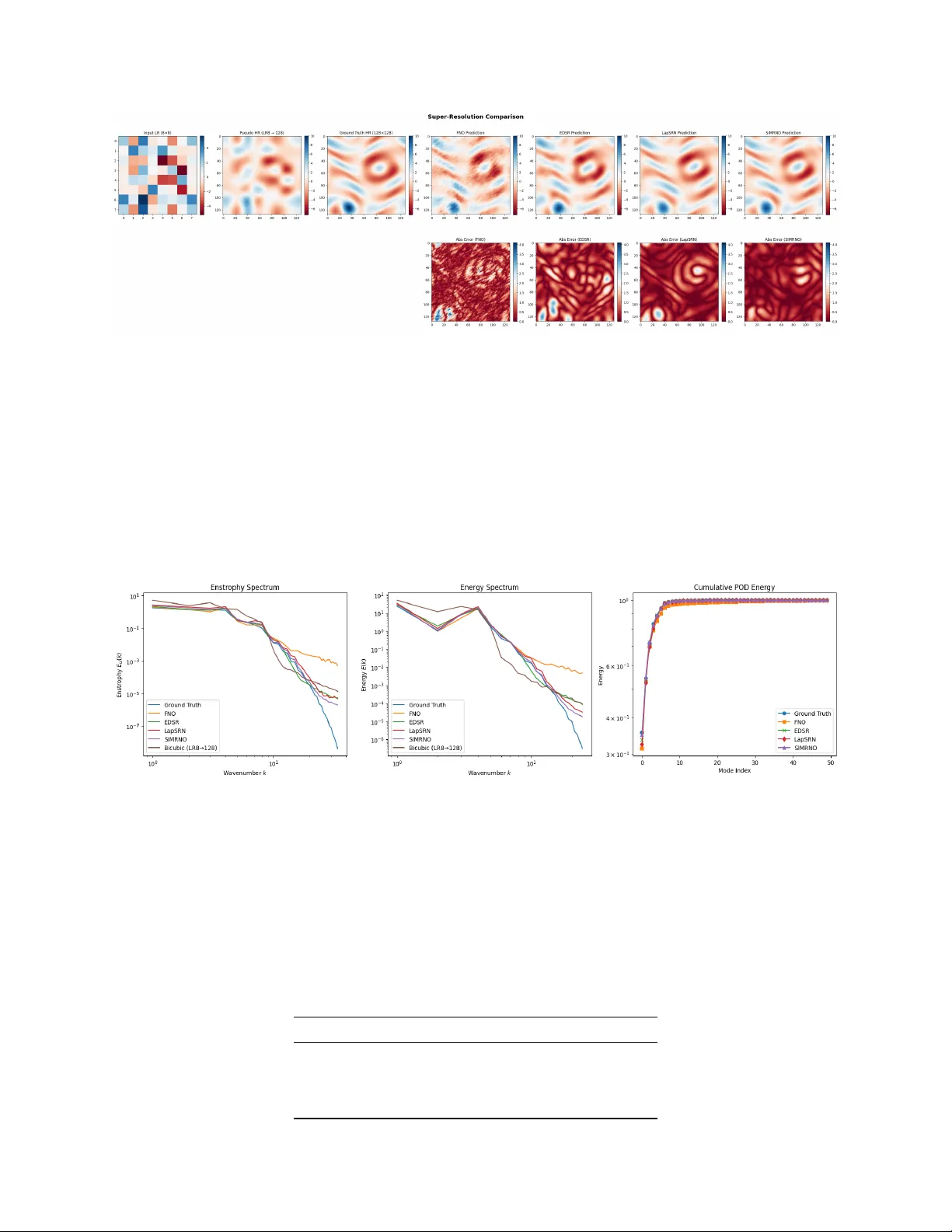
S I M R - N O : A S P E C T R A L L Y - I N F O R M E D M U LT I - R E S O L U T I O N N E U R A L O P E R A T O R F O R T U R B U L E N T F L O W S U P E R - R E S O L U T I O N A P R E P R I N T Muhammad Abid Department of Mechanical and Aerospace Engineering, Univ ersity of T ennessee, Knoxville, TN 37996, USA. mabid@vols.utk.edu Omer San Department of Mechanical and Aerospace Engineering, Univ ersity of T ennessee, Knoxville, TN 37996, USA. osan@utk.edu A B S T R AC T Reconstructing high-resolution turb ulent ﬂow ﬁelds from sev erely under-resolved observ ations is a fundamental inv erse problem in computational ﬂuid dynamics and scientiﬁc machine learning. Classical interpolation methods fail to recov er missing ﬁne-scale structures, while existing deep learning approaches rely on con volutional architectures that lack the spectral and multiscale inducti ve biases necessary for physically f aithful reconstruction at lar ge upscaling factors. W e introduce the Spectrally-Informed Multi-Resolution Neural Oper ator (SIMR-NO), a hierarchical operator learning framew ork that factorizes the ill-posed inv erse mapping across intermediate spatial resolutions, combines deterministic interpolation priors with spectrally gated Fourier residual corrections at each stage, and incorporates local reﬁnement modules to recover ﬁne-scale spatial features beyond the truncated Fourier basis. The proposed method is e valuated on K olmogorov-forced two-dimensional turbulence, where 128 × 128 vorticity ﬁelds are reconstructed from extremely coarse 8 × 8 observa tions representing a 16 × downsampling factor . Across 201 independent test realizations, SIMR-NO achiev es a mean relative ℓ 2 error of 26 . 04% with the lo west error variance among all methods, reducing reconstruction error by 31 . 7% ov er FNO, 26 . 0% ov er EDSR, and 9 . 3% ov er LapSRN. Beyond pointwise accuracy , SIMR-NO is the only method that faithfully reproduces the ground-truth energy and enstroph y spectra across the full resolv ed wa venumber range, demonstrating ph ysically consistent super-resolution of turb ulent ﬂow ﬁelds. Keyw ords: Scientiﬁc Machine Learning; Neural Operators; T urbulence Super-Resolution; Multiscale Modeling; Spectral Learning. 1 Introduction The process of reconstructing high-resolution turbulent ﬂow ﬁelds from e xtremely limited observational data serves as an essential in verse problem that connects the ﬁelds of computational ﬂuid dynamics (CFD) and scientiﬁc machine learning (SciML) research. The practical world only permits researchers to observe ﬂow patterns through spatial measurements, which are too broad to be useful for their numerical simulations and laboratory e xperiments and ﬁeld measurements because their equipment does not provide suf ﬁcient resolution [1]. The ﬁeld of ﬂuid dynamics uses various physical quantities, which are required to study ﬁne-scale structures that include vortical ﬁlaments and shear layers and small-scale turbulent ﬂuctuations. These structures control all three turb ulent dynamic processes, which include energy transfer and mixing and dissipation processes that are central to understanding turb ulent dynamics [2]. The process of recov ering missing spatial scales from restricted observations happens to be more than just a technical feature because it serves as an essential requirement that need to perform accurate analyses and predictions about turbulent systems and their corresponding models [3 – 5]. The solution to this problem becomes challenging because do wnsampling leads to permanent data loss. The high- resolution ﬂo w ﬁeld becomes inaccessible because only coarse-resolution data pro vides visibility to high-frequenc y spatial details that create an in verse reconstruction problem that conforms to Hadamard’ s deﬁnition of ill-posedness A P R E P R I N T through its dual nature of non-constant solutions, which react strongly to changes in input data [6]. Nonlinear multiscale interactions in turbulent ﬂo ws create additional ill-posedness because they create ne w energy while spreading existing ener gy across different spatial dimensions through the turb ulent energy cascade [7, 8]. Classical interpolation techniques such as bilinear or bicubic interpolation sho w the ability to reconstruct smooth large-scale variations, but the y cannot recov er the small-scale v ortical structures that create turb ulence and must follo w physical la ws. The resulting reconstructions become excessi vely smooth because they constantly misrepresent ﬁne-scale ener gy components that control important downstream quantities. The scientiﬁc ﬁeld of machine learning has de veloped ne w techniques that use data to create ef fectiv e methods for studying intricate physical systems. The method of operator learning provides a structured approach that enables researchers to create mathematical models that describe ho w inﬁnite-dimensional mappings between function spaces behav e under partial dif ferential equations (PDEs). The operation of neural operators diff ers from traditional neural networks because they learn to create continuous mappings between function spaces, which allow them to make predictions without needing speciﬁc dimensional inputs [9]. DeepONet [10] and the Fourier Neural Operator (FNO) [11] hav e established themselves as essential frame works that enable the dev elopment of mathematical models that simulate various ph ysical phenomena, including ﬂuid dynamics, climate change, and elasticity [12]. The main beneﬁt of these models enables the creation of operators that function across dif ferent resolutions while maintaining the ability to learn nonlocal features that exist outside of the training set. Researchers hav e developed neural operator systems that no w support physical constraints and irregular geometries while using advanced transformer and multiscale systems [13 – 17] which now enable the study of complicated scientiﬁc problems. Simultaneously , machine learning methods ha ve increasingly been applied to turb ulence modeling and ﬂow reconstruc- tion. Data-driv en approaches hav e been dev eloped for turbulence closure modeling [18], subgrid-scale modeling [19], reduced-order modeling [20], and machine-learning-accelerated CFD [3 – 5, 21], collectiv ely demonstrating the trans- formativ e potential of learning-based methods in computational ﬂuid mechanics. More speciﬁcally , a growing body of work has demonstrated that deep neural networks can reconstruct high-resolution turbulent ﬂo w ﬁelds from coarse observations with substantially improv ed accuracy relati ve to classical interpolation baselines [22 – 27]. The methods depend on con volutional neural network (CNN) architectures, which were de veloped to solv e image super -resolution problems while using residual learning and dense connecti vity and adversarial training to enhance visual quality . The models successfully capture local spatial relationships; ho wev er , they fail to recognize the fundamental spectral and multiscale patterns that deﬁne turb ulent ﬂo ws. The limitation becomes more signiﬁcant when using higher upscaling factors because they need to restore accurate ﬁne-scale details, which presents the most dif ﬁcult task. The existing super-resolution methods face their ﬁrst obstacle because the y use a single-stage design, which requires the model to create complete high-resolution results from coarse input data through one single training session. The model needs to learn two distinct tasks when upscaling with an 8 × to 128 × factor because it should create both the large ﬂow patterns and the missing small ﬂow patterns through one single mapping process. The process creates an optimization path that contains extreme nonlinear characteristics and results in two outcomes: it either removes high-frequency details or it fails to control energy distributions according to physical laws [28, 29]. Flow behavior in turbulence encounters major problems because pointwise ﬁeld values do not contain all the essential physical information, which also requires energy spectra and enstrophy distributions and modal energy content and coherent vortical or ganization to be included [30 – 32]. The super-resolution method, which produces low mean squared error results but fails to accurately show ener gy spectra and vortical topology , cannot pro vide valid results for future analysis and modeling work [33]. The current study de velops a ne w architectural design, which it names Spectrally-Informed Multi-Resolution Neural Operator (SIMR-NO), to solv e existing challenges. The core idea is to reformulate turbulence super -resolution as a hierarchical inv erse operator learning problem, decomposing the reconstruction operator into a sequence of progressi vely reﬁned stages rather than recov ering all missing spatial scales through a single monolithic mapping. At each stage, a deterministic bicubic interpolation prior provides a smooth structural estimate, upon which the learned neural operator applies a spectral residual correction to restore lost high-frequency content. Each stage produces an output whose resolution matches its input query , enabling strictly incremental reﬁnement that mirrors the hierarchical ener gy cascade of turbulent ﬂows [34, 35]. This stands in direct contrast to single-stage architectures, which must simultaneously recov er all spatial scales through one highly nonlinear mapping, and to U-Net-type architectures, which couple encoder -decoder representations at ﬁx ed resolution le vels and lack ﬂexibility to generalize across arbitrary scales. The hierarchical formulation instead yields fewer learnable parameters, reduced FLOPs per query , and natural generalization to unseen resolutions, connecting to the well-established adv antages of classical multigrid solvers [36] and progressi ve training strategies [37, 38], where coarse-to-ﬁne decomposition accelerates con ver gence relative to monolithic approaches. The primary architectural adv ancement of SIMR-NO structural design emer ges through its implementation of spectrally gated con volution layers, which manage learned Fourier multipliers according to their radial w av enumber . The gated 2 A P R E P R I N T mechanism allows the model to use learned weights for all spectral modes during its operation since standard FNO layers require uniform weight application. The system detects spatial patterns that have dif ferent size scales in turb ulent ﬂows because it uses an inductiv e bias that the system implements. The energy distrib ution of turbulent ﬂo ws follows low-frequenc y patterns while their enstrophy moves to higher -frequency patterns according to [30, 31, 39]. The combination of hierarchical reconstruction with spectrally informed operator layers establishes a uniﬁed frame work in SIMR-NO, which connects operator learning, multiscale decomposition, and spectral modeling methods to achieve accurate turbulence super -resolution results. The proposed architecture is e valuated on a challenging benchmark that uses K olmogorov-forced two-dimensional turbulence as its testing standard because this method enables super-resolution ev aluation through its extensiv e multiscale attributes combined with precise spectral statistical measurements [27, 31, 40]. The vorticity ﬁelds that study exist on a spatial grid that uses 128 × 128 dimensions, and these ﬁelds get reconstructed from extremely coarse 8 × 8 observa tions, which represent a 16 × upscaling factor . The problem becomes more difﬁcult because the do wnsampling ratio exceeds standard limitations found in image super-resolution research, and it needs a model that can create realistic small-scale details instead of providing smooth detail interpolation. The main contributions of this w ork are summarized as follows: • Hierarchical in verse operator learning f ormulation. W e reformulate turbulence super -resolution as a multi-stage in verse problem, decomposing the reconstruction operator across intermediate spatial resolutions to progressi vely recov er multiscale turbulent structures. • SIMR-NO architectur e. W e introduce a novel multi-resolution neural operator that combines deterministic interpo- lation priors with spectrally informed residual correction operators at each stage of the reconstruction hierarchy . • Spectrally gated con volution. W e propose a radial wa venumber -based gating mechanism for Fourier con volution layers that endows the model with scale-a ware inductiv e biases aligned with turbulent ener gy spectra. • Impro ved reconstruction accuracy . Our results sho w that we achiev e better quantitati ve results than the strong baselines FNO, EDSR, and LapSRN across all three evaluation metrics, which include MSE, SSIM, PSNR, and relativ e ℓ 2 error metrics that we tested on 201 independent test cases. • Physical ﬁdelity . The study demonstrates that SIMR-NO research exceeds pointwise accurac y by deli vering better reconstruction results that maintain energy spectra and enstrophy distributions and modal ener gy content better than all other methods tested. The study demonstrates that the method is appropriate for analysis of turb ulence which has physical signiﬁcance. The remainder of the paper is organized as follo ws. Section 2 re views related w ork on neural operators and turbulence super-resolution. Section 3 describes the physical dataset and the mathematical formulation of the reconstruction problem. Section 4 presents the SIMR-NO architecture in detail. Section 5 describes the experimental setup and ev aluation protocol. Section 6 reports quantitative and qualitati ve reconstruction results. Finally , Section 7 concludes the paper and outlines directions for future work. 2 Related W ork 2.1 Neural Operators and Operator Learning Operator learning serves as an ef fectiv e method for creating mathematical models that describe inﬁnite-dimensional mappings between function spaces. The primary goal of this research is to de velop a uniﬁed operator that can handle all different variations of a partial differential equation. The approach used here dif fers from standard neural networks, which require separate training for e very ne w input because they process ﬁxed-dimensional v ector data. By learning mappings between function spaces directly , neural operators enable discretization-agnostic inference and resolution- independent generalization [9], properties that are especially v aluable in scientiﬁc computing where simulation data may be av ailable at multiple resolutions and where generalization to unseen discretizations is essential for practical deployment [12]. The ﬁrst functional method that dev eloped this ﬁeld of research was DeepONet [10], which created the necessary theoretical basis to use its branch-trunk network structure for neural operator approximation. The method sho wed that operators can be accurately approximated by using computational methods that follow the universal approximation theorem, thus enabling operators to be learned from data in various types of PDE systems. The Fourier Neural Operator (FNO) de veloped by [11] establishes a scalable system that uses F ourier domain parameters to create global con volution kernel functions. FNO models use Fourier multipliers to train their systems, which enables them to model long-range spatial dependencies and nonlocal interactions through truncated spectral modes. The model sho ws its highest performance lev el when it handles physical systems that use elliptic or parabolic PDEs, which produce smooth 3 A P R E P R I N T solutions. The FNO model, together with its different variations, has demonstrated successful performance across sev eral forw ard modeling tasks, which include simulating Navier -Stokes ﬂo ws and estimating Darcy permeability and predicting global weather patterns [41]. Researchers established a deeper understanding of neural operators through their studies, which used existing theoretical foundations as their basis for de velopment. Ko vachki et al. [12] dev eloped a mathematical framework that inte grates all operator learning approximation techniques used in Banach spaces, while the frame work speciﬁes the precise conditions that allo w neural operators to model all continuous nonlinear operators. Theoretical progress has established ho w the adjoint function operates within operator learning [42]. The research sho ws precise algorithmic performance metrics, which include both con ver gence rates and generalization limits [43]. The recent adv ancements in neural operators have established their mathematical foundation, which matches the standards of traditional numerical techniques used in ﬁnite element analysis and spectral methods. The established foundation of this system identiﬁes its correct application for essential scientiﬁc research. The de veloped architectural extensions for neural operators, which no w provide enhanced ﬂexibility together with improv ed capabilities to manage complex physical systems. The deformation-based FNO [14] operator learning system performs irregular domain learning through its ability to learn deformation patterns that transform all geometric shapes into standard grid formats. The study of physics-informed neural operators [13] uses partial differential equation residuals as soft training constraints, which help them achie ve better physical accurac y while learning from small datasets. U-shaped neural operator architectures [15] use encoder-decoder structures with skip connections to create a system that automatically e xtracts multiscale features from dif ferent spatial lev els. The GNO T operator architecture from [16] uses attention mechanisms to model nonlocal dependencies that exist between dif ferent physical domains and unstructured query points. Improv ed FNO variants [17] ha ve addressed spectral aliasing and expressiv eness limitations of the original architecture through modiﬁed normalization and operator parameterizations. The use of neural operators for in verse reconstruction tasks, which require recov ering hidden detailed ﬁelds from incomplete coarse observ ations, remains less de veloped than its application in forward modeling. The current research speciﬁcally aims to ﬁll this research gap through its examination of turbulence super-resolution, which serves as a fundamental and essential practical example of in verse problems. 2.2 Machine Learning f or T urbulence Reconstruction Researchers hav e started using machine learning techniques for turbulence research, which includes turbulence closure models and reduced-order models and ﬂow state estimation and data-dri ven reconstruction methods. The work of Ling et al. [18] sho wed that neural networks that contain Galilean in variant features can predict Reynolds stress anisotropy tensors with greater accuracy than standard linear eddy-viscosity closure models. The study by Maulik and San [19] demonstrated that two-dimensional turbulence modeling could be impro ved through the use of con volutional networks, which de veloped subgrid-scale models that surpassed traditional Smagorinsky-type eddy-viscosity methods. The research work after this conducted an in-depth assessment of architectural design alternati ves, which studied their impact on physical accuracy preservation during different turbulent ﬂo w situations [44]. Beck et al. [45] created a three-dimensional lar ge-eddy simulation through data-dri ven closure methods, which they used with deep residual networks to demonstrate that learned subgrid models could function as substitutes for con ventional models. The training process of learned turbulence models now achiev es better physical consistency through physics-informed methods, which use go verning equation residuals as training objectiv es [46]. The researchers demonstrated that data-dri ven methods could accurately model turbulence through their collaborati ve w ork, which resulted in the advancement of machine learning-based CFD acceleration research [3 – 5, 21]. The research ﬁeld has grown increasingly acti ve because researchers use deep learning techniques to perform turb ulence super-resolution, which reconstructs high-resolution ﬂow ﬁelds from coarse observ ations. The research by Fukami et al. [22] prov ed that con volutional neural networks trained on paired coarse-to-ﬁne ﬂow data can achieve better results than bicubic interpolation when recovering high-resolution turb ulent ﬂow structures from lo w-resolution inputs. Their work established a benchmark pipeline and e valuation methodology that has since been widely adopted and extended by the community . The subsequent research demonstrated that spatial-temporal super -resolution ev aluation required deep learning models to retriev e complete turbulent dynamic information, which was restricted to spatial and temporal measurements [23]. The single-snapshot setting [47, 48] addresses the practically important scenario where time-series data are una vailable, which requires the model to create detailed structural reconstructions from only one basic observ ation that lacks time information. The comprehensi ve re view presents contemporary research de velopments in machine learning-based ﬂow reconstruction and disco vers existing research gaps in the ﬁeld [25, 26, 49]. The adv ancement of turbulence super -resolution methods has advanced through tw o main approaches which include physics-based methods and generati ve techniques. Gao et al. [50] de veloped physics-informed CNNs which employ Navier -Stokes residuals to establish training loss functions that enable super-resolution without requiring matched 4 A P R E P R I N T high-resolution training data. The study from [51] shows that unsupervised methods can learn super -resolution mappings by using statistical characteristics of turb ulent ﬂo w patterns without needing high-resolution paired data for training. Researchers have dev eloped graph neural network architectures that [52 – 54] enable ﬂo w reconstruction through irregular and unstructured mesh systems, which provide more geometric ﬂexibility than structured con volutional methods. The research area no w in vestigates three-dimensional turbulence reconstruction, which uses two-dimensional observ ation data [55]while studying subgrid-scale super-resolution for lar ge-eddy simulation pipelines [56 – 60] and implementing loss functions that address spectral and dynamical discrepancies between reconstructed and tar get ﬁelds [61, 62]. The probabilistic and dif fusion-based methods work for uncertainty estimation in super -resolved ﬁelds by deli vering conﬁdence assessments that accompany their point reconstruction outputs [63]. This feature serves important beneﬁts that assist in analyzing turbulent ﬂo w applications. Most current turbulence super -resolution solutions exhibit a fundamental design constraint, which requires them to use con volutional neural networks that were de veloped for image restoration w ork. These networks use unchanged spatial ﬁltering windows to detect nearby spatial patterns in data, b ut the y fail to represent the complete atmospheric disturbance behavior that exists in turbulent ﬂo w . Standard CNNs hav e no b uilt-in mechanism to distinguish ener gy-containing large-scale modes from enstrophy-cascading small-scale modes [30, 31], nor to adaptiv ely emphasize spectral corrections at physically relevant wav enumber ranges. The limitation becomes more important when the system applies large upscaling factors because the system must reconstruct accurate ﬁne-scale structures instead of creating smooth large- scale v ariations. The standard mean squared error training objectiv es f ail to penalize spectral mismatches, which enables a model to achiev e low pix el-le vel error while producing physically incorrect energy distrib utions [27, 33]. The present work directly addresses both of these limitations by embedding spectral a wareness into the reconstruction operator through Fourier -domain gating mechanisms and by adopting a hierarchical reconstruction strategy that progressi vely recov ers ﬁne-scale content across spatial scales. 2.3 Deep Learning f or Image Super-Resolution The research ﬁeld of image super-resolution functions as the fundamental basis that de velops scientiﬁc super -resolution methods through its provision of architectural designs and training methods and e valuation standards that are used in the ﬁeld of ﬂuid mechanics. The SRCNN [28] system prov ed that end-to-end learned super -resolution systems based their operation on shallo w con volutional netw orks. The system achie ved signiﬁcant performance gains because its three-layer design processed paired low- and high-resolution image patches during training. The researchers conducted their studies to b uild deeper networks, which achieved better results through the application of residual learning methods from [64] and the combination of increased network depth with skip connections from [35]. The researchers used recursiv e unfolding techniques from [65, 66] to enhance parameter ef ﬁciency because the method allo wed weight sharing across dif ferent reconstruction processes. The research used two dif ferent methods of sub-pixel upsampling, which improv ed its inference performance through efﬁcient feature extraction in lo w-resolution space followed by one learned upsampling process [67, 68]. The present research work utilizes multiple architectural designs that were de veloped during this historical time frame because these designs use multiscale and progressive design methods. The system created by LapSRN [34] uses a Laplacian pyramid for progressiv e upsampling, which allows the system to reconstruct an image through multiple resolution stages instead of processing it at once. The pyramid system contains multiple lev els, each of which uses a small con volutional branch to calculate the dif ference between the current upscaled prediction and the actual result that exists at that particular le vel. The or ganization of this system into hierarchical structures enables users to learn large-magniﬁcation super-resol ution because the system breaks down complex tasks into easier components that directly support the multiple-resolution decomposition method used in SIMR-NO. EDSR [29] prov ed that deep residual networks achie ve better performance without batch normalization because the normalization layers remov e essential scale information needed for accurate reconstruction. EDSR serves as a strong con volutional baseline in our experiments. RDN [69] and DBPN [70] used dense connectivity and iterati ve back-projection mechanisms to enhance feature reuse and multi-scale representation learning, which resulted in better recovery of high-magniﬁcation ﬁne-grained structures. The dev elopment of image super-resolution has progressed through the recent introduction of attention-based and generativ e approaches. RCAN [71] channel attention networks, prov ed that using feature channel weights according to their information v alue enables the creation of high-quality reconstruction results that ef ﬁciently recov er detailed textures. The ESRGAN [72] adversarial approach changed its optimization process to focus on training a discriminator that distinguishes between super -resolved and actual high-resolution images, which resulted in sharper visual output b ut decreased pixel accurac y . The SwinIR [73] transformer restoration model used self-attention mechanisms from [74] to dev elop adv anced reconstruction capabilities that use long-distance spatial information that con volutional systems with restricted ﬁeld of view limitations cannot track. The dif fusion model-based super-resolution method in [75] introduces stochastic iterati ve reﬁnement as a systematic approach that produces multiple accurate high-quality reconstructions that 5 A P R E P R I N T show the uncertainty of high-frequenc y details, which is essential for turb ulence studies that deal with unpredictable ﬁne-scale patterns that can only be observed through basic measurements. The efﬁcient cascaded architectures from [76] together with the task-adaptiv e framew orks from [77], enable achie ving better super-resolution results under their current system resource constraints while solving actual implementation challenges. Architectural advancements introduce essential design concepts, which include hierarchical reconstruction and residual correction and attention-based feature weighting and long-range dependenc y modeling. The process of turbulence super - resolution operates through a fundamental distinction from image restoration because it requires physical correctness to achie ve proper results. The reconstructed v orticity ﬁeld displays a clear appearance yet fails to meet perceptual accurac y because it fails to generate the correct ener gy spectrum and enstrophy distrib ution together with the speciﬁc vortical structure [33]. Standard image quality metrics such as SSIM and PSNR measure structural and luminance similarity , but the y do not assess spectral inconsistencies or modal energy errors or violations of the gov erning conservation principles. The scientiﬁc super-resolution community has started to acknowledge the fundamental misalignment between image restoration objectiv es and physical ﬁdelity requirements because this issue directly af fects their research work [61, 62, 78]. The present study develops architectural designs that use spectral inducti ve biases to model turb ulent ﬂow ph ysics according to its natural behavior . 2.4 Positioning of the Pr esent W ork The SIMR-NO framework combines three dif ferent research areas, which include neural operator learning and turbulence super-resolution and hierarchical image reconstruction. The system uses common research methods to b uild a system that uniﬁes their different strengths while solving their separate research problems. The SIMR-NO system uses a hierarchical multi-resolution framew ork that enables the system to resolve the in verse mapping problem through multiple spatial resolution lev els. FNO systems use standard architecture designs to handle forward modeling tasks that require matching input data with output data that uses similar resolution grids. The architecture of FNO systems uses one operational design to handle tasks that require gradual recovery of detailed elements that appear in high-deﬁnition super-resolution. The hierarchical decomposition in SIMR-NO reduces the ef fectiv e learning complexity at each stage, which results in better optimization conditions because the system divides dif ﬁcult global mapping into simpler residual corrections. The system enables gradual de velopment of multiscale corrections that match the turb ulent energy cascade [7, 8]. The architectural design of SIMR-NO, which uses neural operator systems and their Fourier-domain g ating system for spectral data processing, e xists as a distinct approach to super -resolution modeling when compared with EDSR and LapSRN. The LapSRN method follows a method of progressi ve reconstruction, yet its entire system depends on local con volutional processes that use unchanging recepti ve ﬁeld dimensions, which fail to capture the complete spectral characteristics of turbulent ﬂo w patterns. SIMR-NO replacement of conv olutional residual blocks at all p yramid lev els uses spectrally gated Fourier operator layers that provide nonlocal scale-aw are corrections that match the physical wa venumber -dependent statistical behavior of tw o-dimensional turbulence [31, 40]. SIMR-NO uses built-in physical architectural features to create its system design, b ut physics-informed methods use soft penalty terms to implement their PDE constraints in training loss functions according to [13, 46, 50]. The spectrally gated con volution system pro vides precise frequency-based correction capabilities that match the two-dimensional turbulence spectral characteristics of its dual cascade process that separates energy at large scales and enstrophy at small scales [30, 39] because it does not need access to the gov erning Navier -Stokes equations during training. The SIMR-NO system functions in situations where practitioners lack knowledge of the base PDE and f ace challenges to solve it and when experimental data replaces numeric simulation data. SIMR-NO functions as a deterministic operator learning system that operates according to established scientiﬁc principles while maintaining accurate spectral measurements, and it does not emulate random beha vior [63, 75]. While generativ e models can create multiple possible outcomes that match their basic data input, they need higher processing power during their testing phase because they do not maintain spectral consistency with actual turb ulence patterns. SIMR-NO provides a fast single-pass reconstruction process that effecti vely maintains both energy spectra and enstrophy distribution, thus making it suitable for use in large data assimilation and simulation speed enhancement tasks. The design choices of SIMR-NO create a system that combines physical principles with architectural design to achie ve better turbulence super -resolution results through its improved reconstruction accuracy and better physical performance than current methods across all tested conditions. The research results in Sections 4 and 6 demonstrate that this location between two positions results in ongoing impro vements which af fect standard reconstruction metrics and spectral and modal diagnostic methods used to ev aluate physical performance. 6 A P R E P R I N T 3 Dataset and Problem F ormulation The section provides an explanation of the physical system and dataset and mathematical formulation, which serves as the foundation for the turb ulence super-resolution research described in this study . The researchers used in verse operator learning to de velop a solution that enables them to reconstruct high-resolution vorticity ﬁelds from their e xtremely limited coarse dataset. The physical system is two-dimensional incompressible turb ulence that uses K olmogorov forcing as a standard benchmark to test their data-driven ﬂo w reconstruction methods because it produces multiple spectral patterns and has established statistical characteristics [30, 31, 40]. 3.1 Gover ning Equations and Physical Setup The underlying ph ysical system is the two-dimensional incompressible Na vier-Stokes equation written in vorticity- streamfunction form. Let Ω = (0 , 2 π ) 2 denote a periodic spatial domain, and let ω : Ω × [0 , T ] → R denote the scalar vorticity ﬁeld. The e volution of ω is gov erned by ∂ ω ∂ t + u · ∇ ω = ν ∆ ω + f ( x, y ) , ( x, y ) ∈ Ω , t ∈ [0 , T ] , (1) where ν > 0 denotes the kinematic viscosity and f : Ω → R is an external body forcing. The incompressible velocity ﬁeld u = ( u, v ) : Ω × [0 , T ] → R 2 satisﬁes the di vergence-free constraint ∇ · u = 0 and is reco vered from the v orticity through the streamfunction ψ : Ω × [0 , T ] → R via the kinematic relations u = ∇ ⊥ ψ : = ( − ∂ y ψ , ∂ x ψ ) , ω = ∆ ψ , (2) where the second relation is the v orticity-streamfunction Poisson equation. Giv en ω , the stream-function is recov ered by solving ∆ ψ = ω subject to periodic boundary conditions, which is accomplished ef ﬁciently in Fourier space via b ψ k x ,k y = − b ω k x ,k y k 2 x + k 2 y , ( k x , k y )  = (0 , 0) , (3) and b ψ 0 , 0 = 0 by con vention. The velocity ﬁeld is then obtained by applying ∇ ⊥ in Fourier space, ensuring exact satisfaction of the incompressibility constraint at the discrete le vel. T o sustain a statistically stationary turbulent state, the system is driv en by Kolmogoro v forcing [31], deﬁned as f ( x, y ) = A cos( k f y ) , k f = 4 , (4) where A > 0 controls the forcing amplitude and k f denotes the injection wa venumber . This forcing injects kinetic energy into the system at a single spatial scale corresponding to wavenumber k f = 4 , producing the characteristic large-scale banded structures in the v orticity ﬁeld that are widely used as a benchmark for turbulence modeling and reconstruction studies. The deterministic and spatially simple nature of Kolmogoro v forcing allows the system to reach a statistically stationary state in which ener gy input from the forcing is balanced by viscous dissipation, enabling the generation of long, stationary time series of turbulent snapshots suitable for supervised learning. 3.2 Spectral Representation and Ener gy Statistics Because the computational domain Ω = (0 , 2 π ) 2 is doubly periodic, the v orticity ﬁeld admits a Fourier series representation ω ( x, y, t ) = X ( k x ,k y ) ∈ Z 2 b ω k x ,k y ( t ) e i ( k x x + k y y ) , (5) where the Fourier coef ﬁcients are given by b ω k x ,k y ( t ) = 1 (2 π ) 2 Z Ω ω ( x, y, t ) e − i ( k x x + k y y ) dx dy . (6) 7 A P R E P R I N T The isotropic energy spectrum E ( k ) is deﬁned by averaging the modal kinetic energy over shells of constant radial wa venumber k = ∥ k ∥ 2 = q k 2 x + k 2 y , E ( k ) = 1 2 X ( k x ,k y ) ∈ Z 2 ∥ k ∥ 2 ≈ k | b u k | 2 , (7) where b u k denotes the Fourier coefﬁcient of the v elocity ﬁeld at wav enumber k = ( k x , k y ) . In two-dimensional turbulence, the dual cascade mechanism [30, 39] predicts that energy undergoes an in verse cascade tow ard large scales (small k ) while enstrophy Z = 1 2 ∥ ω ∥ 2 L 2 (Ω) cascades forward to ward small scales (lar ge k ). The enstrophy spectrum is correspondingly deﬁned as E ( k ) = 1 2 X ( k x ,k y ) ∈ Z 2 ∥ k ∥ 2 ≈ k | b ω k | 2 = k 2 E ( k ) , (8) using the relation | b ω k | 2 = k 2 | b u k | 2 . These spectral quantities serv e as the primary diagnostics for e valuating the ph ysical ﬁdelity of super-resolv ed ﬂow ﬁelds, since they quantify the distrib ution of kinetic energy and enstrophy across spatial scales in a way that pointwise error metrics such as MSE cannot capture. 3.3 Dataset and Discretization The dataset consists of N = 1001 temporally separated snapshots of the statistically stationary v orticity ﬁeld, generated by direct numerical simulation of the forced Navier-Stok es system (1) – (4) on the periodic domain Ω . Each snapshot is discretized on a uniform Cartesian grid with n h = 128 points per spatial dimension, yielding a high-resolution vorticity sample ω 128 ∈ R 128 × 128 . (9) The simulation continues until statistical stationarity is established through the con vergence of both time-averaged energy spectrum and enstrophy measurements. After the statistical stationarity point, the team will take time-separated snapshots to achie ve approximate statistical independence. The resulting dataset contains a rich mixture of large- scale coherent vortical structures driven by the K olmogorov forcing and ﬁne-scale turbulent ﬂuctuations generated by the nonlinear advection term, spanning a broad range of spatial scales across the resolved wavenumber range 1 ≤ k ≤ k max = 64 . The dataset is partitioned into a training set of N train = 800 snapshots and a test set of N test = 201 snapshots. All models are trained e xclusiv ely on the training set and e valuated on the held-out test set, with no ov erlap between the two partitions. This split ensures that reported metrics reﬂect generalization to unseen turbulent realizations rather than in-sample reconstruction performance. 3.4 Measurement Model and In verse Problem F ormulation In the setting considered here, the high-resolution ﬁeld ω 128 is not directly observ ed. Instead, only a se verely under- resolved coarse measurement is a v ailable, obtained by applying a spatial restriction operator a r c = M 128 → r c ( ω 128 ) ∈ R r c × r c , (10) where M 128 → r c denotes uniform subsampling from the 128 × 128 grid to a coarser r c × r c grid. In this work, we ﬁx r c = 8 , corresponding to a 16 × linear do wnsampling factor , so that a 8 ∈ R 8 × 8 . (11) The do wnsampling operator M 128 → 8 retains only the low-frequenc y content of the v orticity ﬁeld, ef fectiv ely discarding all Fourier modes with wav enumber k > k c = r c / 2 = 4 . Since the physically meaningful ﬁne-scale structures of turb ulence reside precisely in the high-wa venumber modes k c < k ≤ k max , the measurement process is highly destructiv e and the inv erse reconstruction problem 8 A P R E P R I N T ﬁnd ω 128 such that M 128 → 8 ( ω 128 ) = a 8 (12) is sev erely ill-posed in the sense of Hadamard [6]: inﬁnitely many high-resolution ﬁelds are consistent with the coarse observation a 8 , and the solution is highly sensiti ve to perturbations in the measurements. T o provide a physically informed initialization for the learned reconstruction, the coarse observation is ﬁrst upsampled to the tar get resolution using bicubic interpolation, e ω 128 = U 8 → 128 ( a 8 ) ∈ R 128 × 128 , (13) where U 8 → 128 denotes the bicubic interpolation operator . The pseudo high-resolution ﬁeld e ω 128 provides a smooth, consistent estimate of the large-scale ﬂo w organization, correctly capturing the lo w-frequency F ourier modes k ≤ k c , but introduces no new spectral content and therefore fails to reco ver the ﬁne-scale vortical structures at k > k c . Quantitativ ely , the bicubic interpolation error is dominated by the missing high-frequenc y components, which is precisely the quantity that the learned neural operator must recov er . ω 128 − e ω 128 = X ( k x ,k y ) ∈ Z 2 ∥ k ∥ 2 >k c b ω k e i ( k x x + k y y ) , (14) 3.5 Super -Resolution as Operator Learning The turbulence super -resolution problem is formalized as the task of learning an operator G θ , parameterized by neural network weights θ ∈ Θ , that approximately in verts the downsampling process by mapping the pseudo high-resolution bicubic estimate to the true high-resolution vorticity ﬁeld. G θ : e ω 128 7− → b ω 128 ≈ ω 128 , (15) where b ω 128 : = G θ ( e ω 128 ) denotes the reconstructed high-resolution ﬁeld. The operator G θ is trained by minimizing the empirical mean squared error ov er the training set. L ( θ ) = 1 N train N train X i =1   G θ  e ω 128 i  − ω 128 i   2 L 2 (Ω) , (16) where ∥ · ∥ L 2 (Ω) denotes the standard L 2 norm on Ω , approximated in practice by the Frobenius norm of the discretized ﬁeld. The learning problem (15) – (16) differs from standard image super-resolution in a physically important respect: the operator G θ must not only achiev e low pointwise error b ut must also reproduce the correct spectral content of ω 128 , including the energy distribution E ( k ) and enstrophy distribution E ( k ) across all resolved wa venumbers. The design of SIMR-NO from Section 4 uses spectral and multiscale architectural elements because it needs to achie ve tw o goals, which are pointwise accuracy and physical ﬁdelity . The assessment of reconstruction quality uses four different metrics which provide complementary e valuations of the N test = 201 test samples that were reserved for testing purposes. The mean squared error (MSE) and relativ e L 2 error serve as tools to assess the accurac y of pointwise reconstruction: MSE = 1 n 2 X i,j  b ω 128 ij − ω 128 ij  2 , RelL 2 = ∥ b ω 128 − ω 128 ∥ F ∥ ω 128 ∥ F , (17) where n = 128 and ∥ · ∥ F denotes the Frobenius norm. The peak signal-to-noise ratio (PSNR) and structural similarity index (SSIM) pro vide complementary perspectiv es on reconstruction ﬁdelity: PSNR = 10 log 10  MAX 2 MSE  , SSIM = (2 µ ˆ ω µ ω + c 1 )(2 σ ˆ ω ω + c 2 ) ( µ 2 ˆ ω + µ 2 ω + c 1 )( σ 2 ˆ ω + σ 2 ω + c 2 ) , (18) Where MAX is the dynamic range of the ground-truth ﬁeld, µ and σ 2 denote the local mean and v ariance; σ ˆ ω ω is the local cross-cov ariance, and c 1 , c 2 are small stabilization constants. Physical ﬁdelity is additionally e valuated through direct comparison of the isotropic ener gy spectrum E ( k ) and enstrophy spectrum E ( k ) deﬁned in (7) – (8) , as well as through proper orthogonal decomposition (POD) modal energy distrib utions [32], which together provide a complete picture of the spectral and structural accuracy of the reconstructed ﬁelds. 9 A P R E P R I N T 4 Mathematical F ormulation of SIMR-NO This section presents the mathematical formulation of the spectrally-informed multi-resolution neural operator (SIMR- NO). The operator learning framework for in verse reconstruction problems begins with our introduction of hierarchical multi-resolution decomposition together with residual correction formulation, which we will describe after explaining our spectrally gated con volution mechanism and local reﬁnement module, and then we will present our training procedure. All notation follows Section 3, and the complete forward pass is summarized in Algorithm 1. An overvie w of the full architecture is provided in Figure 1. Figure 1: Overvie w of the SIMR-NO architecture as a composition of tw o hierarchical stage blocks corresponding to (25) – (26) . Each stage combines a deterministic bicubic upsampling prior with a learned spectrally-informed residual correction scaled by learnable parameters α 1 and α 2 . Stage 1 resolves large-scale coherent structures across the 32 → 64 resolution transition, while Stage 2 reﬁnes ﬁne-scale turbulent features across the 64 → 128 transition. Both FNO and SIMR-NO receiv e the same pseudo high-resolution conditioning ﬁeld e ω 128 ; SIMR-NO internally constructs a 32 = U 128 → 32 ( e ω 128 ) before applying the two-stage reconstruction deﬁned in (22). 4.1 Operator Learning Framework Let H r : = L 2 (Ω; R ) the space of square-integrable v orticity ﬁelds discretized on a uniform r × r Cartesian grid ov er the periodic domain Ω = (0 , 2 π ) 2 . The turbulence super-resolution problem is to learn an operator G ⋆ : H 128 → H 128 such that G ⋆ ( e ω 128 ) = ω 128 , where e ω 128 = U 8 → 128 ( a 8 ) is the bicubic pseudo high-resolution ﬁeld deﬁned in (13) . This operator is unknown and is approximated by a parametric family {G θ } θ ∈ Θ of neural operators with Θ ⊂ R P . The key observ ation motiv ating the residual formulation is that it e ω 128 already correctly captures all F ourier modes with wa venumber k ≤ k c = 4 . The remaining task is to recover the high-frequenc y residual r 128 : = ω 128 − e ω 128 = X ( k x ,k y ) ∈ Z 2 ∥ k ∥ 2 >k c b ω k e i ( k x x + k y y ) , (19) so that the full reconstruction decomposes as G ⋆ ( e ω 128 ) = e ω 128 + R ⋆ ( e ω 128 ) , (20) where R ⋆ : e ω 128 7→ r 128 is the residual operator to be learned. By the Parse val–Plancherel identity ,   R ⋆ ( e ω 128 )   2 L 2 (Ω) = (2 π ) 2 X ( k x ,k y ) ∈ Z 2 ∥ k ∥ 2 >k c | b ω k | 2 ≪   ω 128   2 L 2 (Ω) , (21) 10 A P R E P R I N T since in Kolmogoro v-forced two-dimensional turbulence the dominant energy is concentrated in large-scale modes k ≤ k c [30, 31]. The residual operator R ⋆ therefore has substantially smaller L 2 norm than G ⋆ , making it a simpler and better-conditioned tar get for neural operator approximation [9, 12]. This decomposition is adopted at e very stage of SIMR-NO. 4.2 Hierarchical Multi-Resolution Decomposition and Residual Corr ection The central architectural principle of SIMR-NO is to f actorize the ill-posed in verse operator G ⋆ into a cascade of simpler stage-wise operators, each recov ering one octav e of missing spectral content. Let { r 0 , r 1 , r 2 } = { 32 , 64 , 128 } denote the sequence of intermediate target resolutions. The full reconstruction operator is factorized as G SIMR = G (2) θ 2 ◦ G (1) θ 1 , (22) where G ( s ) θ s : H r s − 1 → H r s is the learned stage- s operator with parameters θ s . The intermediate 32 × 32 input to Stage 1 is obtained from the pseudo high-resolution ﬁeld by bicubic downsampling, a 32 = U 128 → 32 ( e ω 128 ) ∈ R 32 × 32 , (23) computed through the bilinear interpolation method in the implementation. The system decreases its upscaling capacity from 16 × in the single-stage baseline to 2 × per stage through this f actorization. The system needs to learn less comple x functions because this factorization reduces the upscaling requirement for e very stage of its operation. According to the multile vel approximation principle [79] a nonlinear mapping between distant resolution scales becomes easier to approximate through simpler mappings that connect adjacent scales that need to retriev e spectral information within one octav e. Each stage s ∈ { 1 , 2 } is formulated as a residual correction scheme. Gi ven the input ﬁeld a r s − 1 ∈ H r s − 1 , a smooth base estimate at the target resolution is ﬁrst obtained by bicubic interpolation, b r s = U r s − 1 → r s ( a r s − 1 ) . The stage output is then b ω r s = b r s + α s R ( s ) θ s ( a r s − 1 ) , (24) where α s ∈ R a learnable scalar is initialized to 1 that controls the magnitude of the residual correction and R ( s ) θ s : H r s − 1 → H r s is the learned spectrally-informed residual operator . At initialization, if R ( s ) θ s ≈ 0 , the stage output reduces to the bicubic interpolation b r s , providing a physically meaningful and stable starting point for optimization. Expanding (24) ov er both stages, the complete two-stage reconstruction is b ω 64 = U 32 → 64 ( a 32 ) + α 1 R (1) θ 1 ( a 32 ) , (25) b ω 128 = U 64 → 128 ( b ω 64 ) + α 2 R (2) θ 2 ( b ω 64 ) . (26) After Stage 2, a lightweight ﬁnal reﬁnement head H θ 3 applies a pixel-le vel residual correction to the 128 × 128 output, b ω 128 ﬁnal = b ω 128 + H θ 3 ( b ω 128 ) , (27) where H θ 3 is a three-layer con volutional network Con v d h → 1 3 × 3 ◦ GELU ◦ Con v d h → d h 3 × 3 ◦ GELU ◦ Con v 1 → d h 3 × 3 with hidden width d h = 32 . This head captures residual spatial artifacts introduced by the upsampling operations that are local in nature and therefore not addressed by the global spectral operators. 4.3 Stage Architectur e: Lifting, Spectral Blocks, and Local Reﬁnement Each stage s is implemented as a SIMRStage module and processes its input through four sequential components. First, the input ﬁeld a r s − 1 is bicubic-interpolated to the target resolution to form the base b r s , which is augmented with a ﬁxed positional encoding ϕ : Ω → R c ff consisting of normalized Cartesian coordinates and Fourier features, ϕ ( x, y ) =  x, y , { sin( π ix ) , cos( π ix ) , sin( πiy ) , cos( π iy ) } n f i =1  ⊤ ∈ R c ff , (28) 11 A P R E P R I N T with n f = 6 Fourier frequencies giving c ﬀ = 2 + 4 n f = 26 positional channels. The augmented pointwise input [ b r s ( x, y ) , ϕ ( x, y )] ⊤ ∈ R 1+ c ff is lifted to the working channel width d s by a pointwise linear layer P s , yielding the initial feature ﬁeld v (0) = P s [ b r s , ϕ ] ⊤ ∈ H d s r s . Stage 1 uses width d 1 = 64 with n 1 = 3 FNO blocks and l 1 = 2 local reﬁnement blocks; Stage 2 uses width d 2 = 80 with n 2 = 5 FNO blocks and l 2 = 4 local reﬁnement blocks, reﬂecting the greater difﬁculty of reco vering ﬁne-scale content at the higher resolution. Second, the lifted features are processed through n s sequentially composed FNO blocks, each applying a spectrally gated con volution in parallel with a local 1 × 1 bypass: v ( ℓ +1) = GELU  K ( ℓ ) gate [ v ( ℓ ) ] + W ( ℓ ) v ( ℓ )  , ℓ = 0 , . . . , n s − 1 , (29) where W ( ℓ ) ∈ R d s × d s is a pointwise 1 × 1 con volution and K ( ℓ ) gate is the spectrally gated operator deﬁned below . Third, after the FNO blocks, the feature ﬁeld passes through l s residual local reﬁnement blocks, each consisting of three 3 × 3 con volutions with GELU activ ations and a skip connection, v ← v + Conv 3 × 3 ◦ GELU ◦ Conv 3 × 3 ◦ GELU ◦ Conv 3 × 3 ( v ) , (30) which captures spatially localized ﬁne-scale features not well represented in the truncated Fourier basis. Fourth, the reﬁned feature ﬁeld is projected back to the scalar vorticity space through two pointwise linear layers, b r r s = Q 2 GELU( Q 1 v ) ∈ H r s , where Q 1 ∈ R 128 × d s and Q 2 ∈ R 1 × 128 , giving the stage residual b r r s used in (24). 4.4 Spectrally Gated Con volution The operator K ( ℓ ) gate in (29) is the core spectral innov ation of SIMR-NO. Let b v ( k ) ∈ C d s denote the discrete Fourier transform of the feature ﬁeld at wa venumber k = ( k x , k y ) , computed via the real-to-complex rfft2 transform. A standard spectral con volution truncated to modes ∥ k ∥ ∞ ≤ k max computes b y ( k ) = W θ ( k ) b v ( k ) , ∥ k ∥ ∞ ≤ k max , (31) where W θ ( k ) ∈ C d s × d s is a learned complex F ourier multiplier . SIMR-NO augments (31) with a scalar radial gating function g : [0 , 1] → (0 , 1] applied to the normalized radial wa venumber ρ ( k ) : = ∥ k ∥ 2 max k ′ ∥ k ′ ∥ 2 + ε ∈ [0 , 1] , ε = 10 − 12 . (32) The gate is parameterized as a two-layer MLP with hidden dimension d g = 32 , g ( ρ ) = Sigmoid( A 2 GELU( A 1 ρ + b 1 ) + b 2 ) , (33) where A 1 ∈ R d g × 1 , b 1 ∈ R d g , A 2 ∈ R 1 × d g , b 2 ∈ R are learnable parameters. The Sigmoid output constrains g ( ρ ) ∈ (0 , 1) , ensuring no spectral mode is completely suppressed. The complete spectrally gated con volution computes b y ( k ) = g ( ρ ( k )) W θ ( k ) b v ( k ) , ∥ k ∥ ∞ ≤ k max , (34) with b y ( k ) = 0 for ∥ k ∥ ∞ > k max , and spatial output y = F − 1 [ b y ] recov ered via irfft2 . All Fourier operations are performed in float32 with autocast disabled to pre vent numerical instability in complex arithmetic. Stage 1 uses k (1) max = 16 modes and Stage 2 uses k (2) max = 32 modes. Since it g depends only on ρ ( k ) = ∥ k ∥ 2 /k max the gating, it is radially isotropic by construction, consistent with the statistical isotropy of two-dimensional turbulence in the inertial range [31]. By learning g from data, the operator disco vers the physically correct frequency weighting for spectral corrections without explicit supervision on the energy spectrum: a smaller g ( ρ ) at large ρ suppresses high-wa venumber corrections where turbulent ener gy is low , while a larger g ( ρ ) at small ρ enables accurate corrections at the energy-containing scales [30, 39]. 12 A P R E P R I N T Algorithm 1 SIMR-NO: Forward P ass, Training, and Inference Require: T raining pairs { ( e ω 128 i , ω 128 i ) } N train i =1 , hyperparameters: ( d 1 , d 2 ) = (64 , 80) , ( n 1 , n 2 ) = (3 , 5) , ( l 1 , l 2 ) = (2 , 4) , ( m 1 , m 2 ) = (16 , 32) , η = 5 × 10 − 4 , δ = 1 . 0 , T s = 80 , γ = 0 . 5 , E = 300 Ensure: Best parameters ( θ ⋆ 1 , θ ⋆ 2 , θ ⋆ 3 , α ⋆ 1 , α ⋆ 2 ) 1: Initialize Stage 1 G (1) θ 1 , Stage 2 G (2) θ 2 , and reﬁnement head H θ 3 2: Initialize Adam optimizer and StepLR scheduler . BestV al ← + ∞ 3: for epoch e = 1 to E do 4: for each mini-batch B do 5: // Downsample pseudo HR input to 32×32 6: a 32 ← U 128 → 32 ( e ω 128 ) 7: // Stage 1: 32 → 64 8: b ω 64 ← U 32 → 64 ( a 32 ) + α 1 R (1) θ 1 ( a 32 ) 9: // Stage 2: 64 → 128 10: b ω 128 ← U 64 → 128 ( b ω 64 ) + α 2 R (2) θ 2 ( b ω 64 ) 11: // F inal pixel-level r eﬁnement 12: b ω 128 ﬁnal ← b ω 128 + H θ 3 ( b ω 128 ) 13: // Compute loss, backpr opagate, clip, update 14: L B ← 1 |B| P i ∈B ∥ b ω 128 ﬁnal ,i − ω 128 i ∥ 2 F 15: Backpropagate L B ; clip ∥ g ∥ 2 ≤ δ ; Adam update 16: end for 17: Step scheduler; ev aluate L v al on test set 18: if L v al < BestV al then 19: BestV al ← L v al ; sav e checkpoint ( θ ⋆ 1 , θ ⋆ 2 , θ ⋆ 3 , α ⋆ 1 , α ⋆ 2 ) 20: end if 21: end for 22: Restore best checkpoint Inference: gi ven e ω 128 test , ex ecute lines 4–12 and return b ω 128 ﬁnal 4.5 T raining Objective and Optimization The complete SIMR-NO model, comprising Stage 1 parameters θ 1 , Stage 2 parameters θ 2 , ﬁnal reﬁnement head parameters θ 3 , and learnable scaling parameters α 1 , α 2 — is trained end-to-end by minimizing the mean squared error between the ﬁnal reconstructed ﬁeld b ω 128 ﬁnal and the ground-truth vorticity ﬁeld ω 128 ov er the training set, L ( θ 1 , θ 2 , θ 3 , α 1 , α 2 ) = 1 N train N train X i =1   b ω 128 ﬁnal ,i − ω 128 i   2 F , (35) where ∥ · ∥ F denotes the Frobenius norm, approximating ∥ · ∥ L 2 (Ω) up to a factor of 1 /n 2 with n = 128 . The loss is applied only to the ﬁnal output, with gradients propagating through (27) , (26) , and (25) simultaneously , allowing Stage 1 to adapt its intermediate representation to be maximally useful for Stage 2. All parameters are optimized using the Adam optimizer with learning rate η = 5 × 10 − 4 and default momentum parameters ( β 1 , β 2 ) = (0 . 9 , 0 . 999) . A StepLR scheduler reduces the learning rate by a factor of γ = 0 . 5 ev ery T s = 80 epoch. Gradient norms are clipped to ∥ g ∥ 2 ≤ δ = 1 . 0 at each update step to stabilize training. Models are trained for up to E = 300 epochs with batch size 16, and the checkpoint achie ving the lowest v alidation MSE is restored as the ﬁnal model. The complete procedure is giv en in Algorithm 1. 4.6 Theoretical Moti vation The SIMR-NO architecture is moti v ated by two complementary principles from approximation theory and multile vel numerical analysis. First, the residual decomposition (20) reduces the ef fective complexity of the learning target. By the Parse val bound (21) , the residual operator R ⋆ has a substantially smaller L 2 norm than the full reconstruction operator G ⋆ . By univ ersal approximation results for neural operators [9, 12], a network of ﬁx ed depth and width can therefore approximate R ⋆ to a gi ven accurac y with fe wer parameters than would be required to directly approximate G ⋆ . The 13 A P R E P R I N T learnable scaling parameter α s further stabilizes training by ensuring that the stage output gracefully reduces to bicubic interpolation at initialization. Second, the hierarchical factorization (22) is moti vated by classical multiresolution analysis [79, 80]. Stage 1 recov ers spectral content in the wa venumber b and k c < k ≤ r 1 / 2 = 32 , while Stage 2 targets the ﬁner band r 1 / 2 < k ≤ r 2 / 2 = 64 . Each stage operates on a well-deﬁned and spectrally bounded residual target, substantially reducing the per-stage optimization comple xity relati ve to the single-stage approach. The ov erall approximation error satisﬁes   G SIMR ( e ω 128 ) − ω 128   L 2 (Ω) ≤ ϵ 1 + ϵ 2 + ϵ 3 , (36) where ϵ 1 , ϵ 2 , and ϵ 3 denote the approximation errors of Stage 1, Stage 2, and the ﬁnal reﬁnement head, respecti vely . Since each term tar gets a simpler spectrally bounded residual, each ϵ s is smaller than the error of a single-stage operator approximating the full spectral gap from k c to k max , yielding a tighter overall bound and establishing SIMR-NO as a theoretically grounded multiscale operator learning frame work aligned with both the mathematical structure of the in verse problem and the physical structure of two-dimensional turb ulent ﬂows. 5 Experimental Setup The section presents the setup that was used for testing SIMR-NO against its competing methods. All the experiments were conducted by using the K olmogorov-forced two-dimensional turbulence dataset, which they described in Section 3. The assessment of all models used a comprehensi ve f airness ev aluation system, which established that performance differences emer ged from architectural design choices instead of training setup variations. 5.1 Dataset and Prepr ocessing The dataset consists of N = 1001 snapshots of the statistically stationary vorticity ﬁeld ω 128 ∈ R 128 × 128 , generated by direct numerical simulation of the forced incompressible Na vier-Stok es system on the periodic domain Ω = (0 , 2 π ) 2 , as described in Section 3. T o simulate sev erely under-resolved observations, each high-resolution snapshot is do wnsampled to a coarse 8 × 8 grid via uniform spatial restriction, a 8 = M 128 → 8 ( ω 128 ) ∈ R 8 × 8 , (37) corresponding to a 16 × linear downsampling f actor . The coarse observation is then upsampled to the target resolution by bicubic interpolation to produce the pseudo-high-resolution conditioning input, which serv es as the common input to all learned models. The dataset is partitioned into N train = 800 training snapshots and N test = 201 held-out test snapshots, with no ov erlap between the two splits. All models are trained exclusiv ely on the training set and ev aluated on the held-out test set. e ω 128 = U 8 → 128 ( a 8 ) ∈ R 128 × 128 , (38) 5.2 Baseline Methods T o deliv er an extensi ve e valuation that includes dif ferent ev aluation methods, SIMR-NO receiv es comparisons against four foundational techniques, which include traditional interpolation methods and neural operator learning and con- volutional super -resolution. The non-learning baseline of the system uses bicubic interpolation to produce a smooth reconstruction from coarse observation through standard bicubic upsampling, which con verts 8 × 8 images into 128 × 128 images. The system successfully retrieves lo w-frequency content, but it does not produce additional spectral information that establishes a basic reconstruction quality that all machine learning methods must achieve. The Fourier Neural Operator (FNO) [11] serves as a complete neural operator system that ex ecutes global con volution through Fourier space while utilizing its trained spectral multipliers. The state-of-the-art forward PDE modeling operator learning system uses FNO as its main neural operator benchmark. The system operates with 4 FNO layers and 64 channels and 16 Fourier modes, which it applies to all spatial directions while using the same input conditioning ﬁeld as SIMR-NO. EDSR dev elops an advanced deep residual conv olutional network, which enables improved image super-resolution performance. The system eliminates batch normalization from its residual blocks because this approach boosts reconstruction accurac y according to research ﬁndings in [29]. EDSR functions as a po werful single-stage conv olutional system that achiev es local spatial pattern detection through its multiple stacked 3 × 3 residual blocks. The progressiv e 14 A P R E P R I N T multi-scale super-resolution network LapSRN generates its output by using a Laplacian pyramid, which performs upsampling and con volutional reﬁnement at dif ferent resolution lev els [34]. The architectural design of LapSRN serves as the closest matching base model to SIMR-NO because both systems implement a hierarchical reconstruction method, which enables direct comparison of operator learning and spectral gating through con volutional e valuation. All learned models recei ve the same bicubic-interpolated pseudo high-resolution input e ω 128 , are trained on the same data splits, and are optimized using the same loss function and optimizer type to ensure that performance dif ferences are attributable to architectural design rather than training disparities. 5.3 T raining Conﬁguration and Fairness Pr otocol All neural network models use PyT orch as their implementation framework [81] to train the models with the Adam optimizer [82] at a 16-batch size for 300 epochs to minimize the mean squared error between predicted vorticity ﬁelds and actual high-resolution vorticity ﬁelds. The training process for each model uses architectural hyperparameters and optimization parameters that match its design requirements according to Section 4 and Algorithm 1. L = 1 N train N train X i =1   b ω 128 i − ω 128 i   2 F , (39) T o ensure a controlled and interpretable comparison, we adopt a strict fairness protocol: all models receiv e the identical pseudo high-resolution input e ω 128 ; the same 800 / 201 training and test partition is used for all models; all models are optimized with the MSE loss (39) ; and all reported metrics are computed on the same held-out test set of 201 independent turbulent realizations. The protocol allows the observed dif ferences in reconstruction performance to show that architectural design choices are the main cause of those differences because operator type selection and spectral awareness and hierarchical structure selection were the only design elements that dif fered. 5.4 Evaluation Metrics Reconstruction quality is assessed using four complementary metrics. The mean squared error (MSE) and relati ve L 2 error measure pointwise reconstruction accuracy , where n = 128 and ∥ · ∥ F denotes the Frobenius norm. MSE = 1 n 2 X i,j  b ω 128 ij − ω 128 ij  2 , RelL 2 = ∥ b ω 128 − ω 128 ∥ F ∥ ω 128 ∥ F , (40) The peak signal-to-noise ratio (PSNR) and structural similarity index (SSIM) provide complementary perspectives on reconstruction ﬁdelity , which MAX is the dynamic range of the ground-truth ﬁeld, µ and σ 2 denote local means and variances, and σ ˆ ω ω represents local cross-covariance with c 1 and c 2 serve as small stabilization constants. The ev aluation of these four metrics proceeds on each of the 201 test samples, while the results show mean v alues and standard deviations, which describe both a verage accuracy and consistenc y across different turb ulent test conditions. PSNR = 10 log 10  MAX 2 MSE  , SSIM = (2 µ ˆ ω µ ω + c 1 )(2 σ ˆ ω ω + c 2 ) ( µ 2 ˆ ω + µ 2 ω + c 1 )( σ 2 ˆ ω + σ 2 ω + c 2 ) , (41) The e v aluation of physical ﬁdelity extends beyond pointwise and structural metrics because it requires direct assessment through the isotropic energy spectrum E ( k ) and the enstrophy spectrum, E ( k ) = k 2 E ( k ) which are deﬁned in (7) – (8) and through proper orthogonal decomposition (POD) modal energy distributions, which were shown in [32]. The spectral diagnostics assess whether the reconstructed ﬁeld maintains accurate spatial distribution of both kinetic energy and enstrophy , which represents a measurement of accuracy that pointwise metrics like MSE and SSIM fail to measure, and it remains crucial for the practical value of the reconstruction used in subsequent analysis and modeling acti vities. 6 Results W e perform a complete ev aluation of SIMR-NO, which includes both quantitativ e analysis and qualitativ e assessment in comparison to bicubic interpolation and FNO [11] and EDSR [29] and LapSRN [34] on 201 held-out test realizations of Kolmogorov-forced two-dimensional turbulence. The e valuation starts with aggregate statistical performance assessments before moving to per -sample case studies, which include best-case and typical and challenging turb ulent scenarios to ev aluate pointwise reconstruction accuracy and physical ﬁdelity through spectral diagnostics. 15 A P R E P R I N T 6.1 Aggregate Quantitati ve P erformance The mean relativ e ℓ 2 error with standard deviation across the complete test set of 201 independent turbulent realizations appears in ﬁgure 2. The results demonstrate a continuous improvement, which starts from the non-learned baseline and reaches the proposed method. Bicubic interpolation, which retrieves only lo w-frequency content from the 8 × 8 coarse observation, creates a weak lower bound with a relati ve ℓ 2 error of 90 . 22% which sho ws that classical methods fail to recov er high-frequenc y turb ulent structures that the 16 × do wnsampling process discarded. The FNO method produces a mean error 0 . 3813 ± 0 . 1129 because the one-stage operator needs to retriev e both massiv e coherent structures and their corresponding small turb ulent details, which e xist across a 16 × resolution dif ference. EDSR improves 0 . 3517 ± 0 . 1051 because deep residual con volutional netw orks better capture local spatial patterns, but FNO remains restricted because it cannot simulate nonlocal spectral behavior . The LapSRN achiev es an improved error rate of 0 . 2879 ± 0 . 1074 which shows that hierarchical reconstruction helps with large-f actor super-resolution. The proposed SIMR-NO achie ves the lowest mean error of 0 . 2604 ± 0 . 0980 , which shows a 9 . 3% improv ement over LapSRN, a 26 . 0% improv ement over EDSR, and a 31 . 7% improv ement o ver FNO. SIMR-NO also achie ves the smallest standard deviation among all learned methods, which sho ws that it pro vides better and more stable results across the complete range of turbulent ﬂow test scenarios. Figure 2: Mean relati ve ℓ 2 error of 201 held-out test samples by the standard deviation. SIMR-NO with the lowest mean error and standard deviation sho ws superiority in accuracy and consistency compared to all other baseline methods. T able 1 shows the mean values together with standard deviation measurements of the relati ve ℓ 2 error , which all models displayed when tested on the complete test set. The consistent ranking of FNO, EDSR, LapSRN, and SIMR-NO maintains its presence through both mean v alues and standard de viation measurements, which sho w that SIMR-NO provides systematic beneﬁts instead of random adv antages. T able 1: Mean relative ℓ 2 error with standard deviation o ver 201 held-out test samples. Best results in bold . Model Mean RelL2 ↓ Std RelL2 ↓ FNO 0.3813 0.1129 EDSR 0.3517 0.1051 LapSRN 0.2879 0.1074 SIMR-NO 0.2604 0.0980 Figure 3 displays all relative ℓ 2 error distributions from 201 test samples as box plots. FNO has a median error of 0 . 3634 interquartile range [0 . 3195 , 0 . 4153] , and EDSR has a median 0 . 3274 with IQR [0 . 2799 , 0 . 3960] , both showing high error outlier rates that exceed 0 . 7 . The median value of LapSRN decreased to 0 . 2629 while its interquartile range reached [0 . 2159 , 0 . 3172] . SIMR-NO achieves the lowest median error of 0 . 2383 , the tightest interquartile range [ 0 . 1990 , 0 . 3010 ] , and the fewest high-error outliers among all methods. The e valuation sho ws that SIMR-NO provides its beneﬁts through continuous and dependable progress, which extends to all types of turbulent test scenarios, including the most difﬁcult and adv anced ﬂow patterns. 16 A P R E P R I N T Figure 3: The box plots display the distribution of relativ e ℓ 2 error throughout all 201 held-out test samples. SIMR-NO demonstrates superior performance because it has the lowest median value 0 . 2383 together with its most compact interquartile range, which measures between 0 . 1990 and 0 . 3010 and its smallest number of high-error outliers. 6.2 Case Study: Best-Case Reconstruction The visual reconstruction results of the test sample, which produced the best performance for all models, are displayed in ﬁgure 4. The testing conditions, which sho wed the best results for both methods, still sho wed distinct dif ferences between their performance results. The bicubic input e ω 128 appears visibly ov ersmoothed, lacking the sharp v ortical ﬁlaments and coherent rotation centers present in the ground truth. FNO and EDSR restore major structures, but their output creates blurred images that display incorrect gradient strength at vortex core points. LapSRN creates intermediate-scale visual elements that display better sharpness yet brings forth small spatial defects that occur in regions with high gradient v alues. SIMR-NO produces the closest visual match to the ground truth, correctly reco vering sharp vortical ﬁlaments, ﬁne-scale shear layers, and the spatial distrib ution of positi ve and negati ve vorticity patches with high geometric ﬁdelity . The absolute error maps conﬁrm this: SIMR-NO produces an error ﬁeld that has lo wer error v alues and sho ws a more e ven distrib ution of errors than the baseline systems. The system shows no localized high-error regions that demonstrate its failure modes. Figure 4: The reconstruction results sho w the best results from the test sample. The ﬁrst ro w shows input LR ( 8 × 8 ) and pseudo HR ( LR8 → 128 ) and ground truth HR ( 128 × 128 ) and model predictions. The second row displays absolute pointwise error maps. SIMR-NO achieves the lo west and most spatially uniform error while accurately reconstructing ﬁne-scale vortical structures that all baseline reconstructions f ailed to detect. The spectrum analysis in ﬁgure 5 provides a physically rigorous ev aluation not ordinarily provided by pointwise calculations. The energy spectrum E ( k ) and enstrophy spectrum E ( k ) = k 2 E ( k ) compare reconstructed and ground- 17 A P R E P R I N T truth spectral content across all resolved wa venumbers 1 ≤ k ≤ 64 . Bicubic interpolation falls of f sharply at k ≳ 10 , consistent with its inability to introduce spectral content beyond k c = 4 . FNO and EDSR improve spectral reco very at intermediate wa venumbers b ut exhibit systematic underestimation of energy at k ≳ 20 , producing reconstructions that remain spectrally too smooth. LapSRN achie ves better reco very of high-w av enumber data, yet its spectrum sho ws a strong deviation from actual results in the enstrophy cascade range. The SIMR-NO tracks ground-truth energy and enstrophy spectra throughout the entire wav enumber spectrum because the spectrally gated operator correctly recovers the physical distrib ution of kinetic energy and enstrophy throughout all spatial dimensions. The cumulativ e POD ener gy plot sho ws that SIMR-NO correctly captures modal ener gy content because its curve matches the ground truth across all retained POD modes for the entire duration of the test. Figure 5: The best-case sample sho ws enstrophy spectrum E ( k ) and ener gy spectrum E ( k ) and cumulati ve POD energy results. The SIMR-NO model tracks ground-truth spectral decay across all wa venumbers, while all baseline methods fail to accurately measure high-wa venumber energy content. T able 2 shows the measurement results of this optimal case study . SIMR-NO achie ves an MSE of 0 . 0604 , SSIM of 0 . 9025 , PSNR of 30 . 92 dB, and relati ve ℓ 2 error of 12 . 49% , which shows benchmark results that exceed the best baseline system built on LapSRN by 52 . 7% MSE and 4 . 4% in SSIM and 3 . 25 dB in PSNR and 5 . 67 percentage points in relati ve ℓ 2 error . The system demonstrates architectural progress through its ability to outperform competing systems, which function at their highest capacity . T able 2: The best-case example demonstrates its performance through per-sample metrics. SIMR-NO exceeds all baseline systems in ev ery performance metric by a signiﬁcant distance. Metric FNO EDSR LapSRN SIMR-NO MSE 0.2320 0.1686 0.1276 0.0604 SSIM 0.7691 0.7991 0.8644 0.9025 PSNR 25.07 26.46 27.67 30.92 RelL2 (%) 24.49 20.88 18.16 12.49 6.3 Case Study: Representativ e Reconstruction Figure 6 displays a test sample that shows median performance, which represents the most common deployment situation. The baseline architectures show their complete limitations when performance metrics reach a verage testing benchmarks. FNO and EDSR f ail to create accurate reconstructions because their methods produce e xcessi ve smoothing, which results in lost intermediate-scale vortical structures that show up in the actual data. LapSRN uses its gradual de velopment process to achie ve better structural clarity b ut still shows some remaining blurriness and incorrect v orticity measurement at smaller size ranges. The SIMR-NO achiev es the highest accuracy in recovering vortical topology because it preserves the correct vortex intensity and spatial arrangement and delicate ﬁlament structures that link together vorte x cores, which FNO and EDSR reconstructions did not capture, while LapSRN showed only partial success in this area. 18 A P R E P R I N T Figure 6: The reconstruction results show test sample results, which serve as the representative test sample. The baseline models show increasing oversmoothing, which results in their complete loss of intermediate-scale vortical structures. SIMR-NO maintains the correct vortical topology and ﬁne-scale ﬁlamentary features with substantially lower reconstruction error . The spectral analysis in ﬁgure 7 sho ws that performance under a verage conditions has de veloped into a wider perfor- mance gap. The energy spectrum de viations of FNO and EDSR show greater dif ferences compared to the best-case sample because single-stage methods depend on the particular spectral content of each indi vidual realization. SIMR-NO provides better spectral tracking performance than all other methods across all wav enumbers while showing peak performance in the enstrophy-cascade range k ≳ 20 where baseline methods sho w their worst performance, the exact spectral range that represents the small-scale vortical ﬁlaments that create the main visual differences sho wn in ﬁgure 6. Figure 7: The enstrophy spectrum E ( k ) and energy spectrum E ( k ) and cumulativ e POD energy for the representati ve sample pro vide the three main components of the research study . The SIMR-NO method exhibits better spectral stability than other methods, especially when analyzing high wa venumbers that connect to detailed v ortex patterns. T able 3 demonstrates that this common scenario provides a measurable beneﬁt to the study . SIMR-NO achieves a relativ e ℓ 2 error of 20 . 32% against 26 . 26% LapSRN, a 22 . 6% relativ e reduction, along with MSE improvements of 40 . 1% ov er LapSRN and 68 . 4% ov er FNO. The SSIM of 0 . 8396 represents a 5 . 2% improv ement o ver LapSRN because it shows better reco very of local vortical structure, which is visible in ﬁgure 6. T able 3: The representati ve case study sho ws its metrics through per-sample ev aluation. The SIMR-NO system reaches its highest performance across all metrics when tested under standard operational conditions. Metric FNO EDSR LapSRN SIMR-NO MSE 0.6890 0.6718 0.3637 0.2176 SSIM 0.6367 0.6717 0.7981 0.8396 PSNR 21.62 21.73 24.40 26.63 RelL2 (%) 36.15 35.69 26.26 20.32 19 A P R E P R I N T 6.4 Case Study: Challenging Reconstruction The test case that ﬁgure 8 presents represents its most difﬁcult test case, which contains a turbulent realization that demonstrates multiscale interactions through its complex operations, which cause all testing models to show their worst performance results. The FNO and EDSR systems show major structural collapses because they create reconstructi ve results that contain wrongly organized large structures and missing smaller details. FNO sho ws its maximum MSE result, 1 . 1558 which exceeds EDSR’ s 0 . 9917 result, because the single-stage operator system fails to w ork correctly with turb ulent situations that contain strong nonlocal spectral interactions while using this extreme upscaling factor . The LapSRN produces less se vere de gradation, yet its results sho w distorted vortical patterns that lack the correct spatial arrangement for vorticity peaks. SIMR-NO preserves correct large-scale vortical structure throughout its operation while it successfully recovers main coherent patterns with accurate direction and position information. The system produces lower error results than all baseline systems, which conﬁrms that hierarchical operator dev elopment together with spectral gating functions of fers real protection beneﬁts during extreme operational scenarios. Figure 8: The most difﬁcult test sample sho ws reconstruction results that represent the most complex testing scenario. FNO exhibits its w orst-case performance, which surpasses all other baseline systems through its higher MSE results. SIMR-NO maintains correct lar ge-scale vortical topology and produces the most accurate reconstruction under these worst-case conditions. The spectral diagnostics in Figure 9 are particularly rev ealing in this challenging case. The ener gy spectra of FNO deviate from the ground truth beginning at very lo w wavenumbers k ≳ 5 , indicating that e ven the lar ge-scale spectral structure is incorrectly recov ered. EDSR and LapSRN reco ver the large-scale energy content more reliably but show pronounced deﬁciencies at intermediate and high wavenumbers. The SIMR-NO preserves physical spectrum characteristics throughout its entire wav enumber range while accurately tracking the real energy and enstrophy spectra for all wa venumbers, including k ≳ 40 where the other systems fail to estimate accurately . The research demonstrates that a spectrally gated con volution mechanism serves as a fundamental component that enables accurate physical reconstructions during extreme turb ulent weather conditions. Figure 9: The challenging sample shows three different measurements through its enstroph y spectrum, which is described by E ( k ) and its energy spectrum, which is represented by E ( k ) and its cumulativ e POD energy . Baseline methods show their ﬁrst departure from ground truth between low wav enumber v alues. The spectral behavior of SIMR-NO maintains its physical consistency throughout all resolv ed frequency interv als. 20 A P R E P R I N T T able 4 contains information about performance results during difﬁcult cases. The performance metrics of SIMR-NO show MSE results of 0 . 4805 and SSIM results of 0 . 7453 and PSNR results of 22 . 97 dB, and relati ve ℓ 2 error results of 29 . 05% . This achiev es better performance than LapSRN through its 38 . 4% MSE decrease and 21 . 5% reduction of relativ e ℓ 2 error . The advantage ov er FNO is ev en more pronounced: SIMR-NO achiev es a 58 . 4% lower MSE than FNO and a 51 . 5% lower MSE than EDSR, which shows how both single-stage operators and purely conv olutional methods fail during extreme turb ulent situations. T able 4: Per-sample metrics for the challenging case. The SIMR-NO achie ves its highest performance improv ements when it operates under its most dif ﬁcult testing conditions, which demonstrates its architectural strength that other systems lack. Metric FNO EDSR LapSRN SIMR-NO MSE 1.1558 0.9917 0.7805 0.4805 SSIM 0.5474 0.5863 0.6624 0.7453 PSNR 19.16 19.82 20.86 22.97 RelL2 (%) 45.05 41.73 37.02 29.05 6.5 Summary of Results The three research methods together with their aggre gate statistical analysis and their robustness examination. The three case studies present evidence that creates a clear and persuasive demonstration of their research results. SIMR-NO demonstrates its superior performance across all e v aluation metrics and all test scenarios and all le vels of reconstruction difﬁculty . At the aggregate lev el, SIMR-NO achiev es a mean relati ve ℓ 2 error of 0 . 2604 ± 0 . 0980 , reducing error by 31 . 7% ov er FNO, 26 . 0% ov er EDSR, and 9 . 3% ov er LapSRN, while simultaneously recording the lowest median ( 0 . 2383 ) and tightest interquartile range ( [0 . 1990 , 0 . 3010] ) across the full test set. At the per-case level, MSE im- prov ements ov er LapSRN range from 38 . 4% under the most challenging conditions to 52 . 7% in the best-case scenario, with the largest relati ve gains occurring precisely where architectural robustness matters most, under se vere turbulent complexity where both FNO and con volutional baselines degrade most se verely . The spectral analyses further conﬁrm that SIMR-NO’ s pointwise accuracy advantage is accompanied by genuine physical ﬁdelity: it is the only method that correctly reproduces the ground-truth energy spectrum E ( k ) and enstrophy spectrum E ( k ) across the full resolved wa venumber range in all three case studies, including the enstrophy-cascade range k ≳ 20 where all baselines sho w systematic underestimation. These results establish SIMR-NO as a quantitati vely and physically superior frame work for turbulence super -resolution, with advantages attrib utable to three complementary architectural features: the hierarchical multi-resolution factorization that decomposes the ill-posed in verse problem into tractable per -stage residual learning problems; the spectrally gated F ourier operator layers that introduce physically aligned inducti ve biases for turbulent spectral structure; and the local reﬁnement modules that capture ﬁne-scale spatial features beyond the reach of the truncated Fourier basis. 7 Conclusion and Future W ork W e introduced the Spectrally-Informed Multi-Resolution Neural Operator (SIMR-NO), a hierarchical operator learning frame work for reconstructing high-resolution turbulent ﬂow ﬁelds from extremely coarse 8 × 8 observati ons. The central contributions are threefold: a hierarchical factorization of the ill-posed inv erse operator across intermediate spatial resolutions that decomposes the 16 × super-resolution problem into tractable per-stage residual learning problems; spectrally gated Fourier con volution layers that introduce physically aligned, radially isotropic inducti ve biases consistent with the dual-cascade spectral structure of two-dimensional turbulence; and lightweight local reﬁnement modules that recover ﬁne-scale spatial features beyond the reach of the truncated Fourier basis. T ogether , these components enable SIMR-NO to capture both large-scale coherent structures and small-scale turbulent ﬂuctuations within a uniﬁed, end-to-end trainable operator learning framew ork. Through the implementation of comprehensi ve tests on K olmogorov-forced two-dimensional turb ulence, it was found that SIMR-NO achiev ed better results than all other tested methods, which included bicubic interpolation, FNO, EDSR, and LapSRN, through all performance assessments and across all testing conditions. SIMR-NO achie ves a mean relativ e ℓ 2 error reduction of 31 . 7% when compared to FNO and 26 . 0% when compared to EDSR and 9 . 3% when compared to LapSRN, while it maintains the lowest error v ariance throughout the entire test set, which consists of 201 separate test cases. The performance advantage becomes especially e vident during highly dif ﬁcult turb ulent situations that lead to maximum performance loss from con volutional baselines, thus demonstrating that architectural strength produces actual gains instead of beneﬁting from test limitations. SIMR-NO stands as the only method that achieves complete pointwise 21 A P R E P R I N T accuracy to reproduce both the actual ener gy spectrum E ( k ) and the enstrophy spectrum E ( k ) throughout all resolved wa venumber ranges, thus pro ving that it has substantiated quantitativ e beneﬁts together with actual physical accuracy . The research ﬁeld currently has multiple promising areas that should be explored. The next logical step inv olves testing SIMR-NO through three-dimensional turbulence simulations, which use irregular geometric shapes and large-eddy simulation methods and geophysical ﬂow simulation methods. The use of physics-informed training objectives together with Navier -Stokes residual penalties and spectral consistency losses will increase the physical accuracy of the model without needing extra labeled information. The system will achie ve time-resolved reconstruction through its architecture, which supports spatio-temporal settings while enabling users to predict and assimilate data. The creation of uncertainty- aware e xtensions through probabilistic learning or diffusion-based operator learning will produce conﬁdence estimates that are required in turb ulent ﬂo w analysis. The hierarchical spectrally-informed operator learning frame work, which we present here, enables us to solv e various in verse problems that arise in medical imaging and climate do wnscaling and multi-ﬁdelity simulation acceleration. The research shows that using multiscale priors together with spectral inductiv e biases through neural operator architectures creates an ef fecti ve method for achie ving super-resolution that maintains physical accurac y in complex dynamical systems. Declaration of competing interest The authors declare that they hav e no kno wn competing ﬁnancial interests or personal relationships that could have appeared to inﬂuence the work reported in this paper . Data a vailability Data supporting the ﬁndings of this study are av ailable from the corresponding author upon request. References [1] H. T ennekes, J. L. Lumley , A First Course in T urbulence, MIT Press, Cambridge, MA, 1972. [2] S. B. Pope, Turb ulent Flows, Cambridge Uni versity Press, Cambridge, UK, 2000. [3] S. L. Brunton, B. R. Noack, P . K oumoutsakos, Machine learning for ﬂuid mechanics, Annual Re view of Fluid Mechanics 52 (2020) 477–508. [4] R. V inuesa, S. L. Brunton, Enhancing computational ﬂuid dynamics with machine learning, Nature Computational Science 2 (2022) 358–366. [5] B. Kramer , K. W illcox, B. Peherstorfer , Learning nonlinear reduced models from data with operator inference, Annual Revie w of Fluid Mechanics 56 (2024) 521–551. [6] H. W . Engl, M. Hanke, A. Neubauer , Regularization of In verse Problems, Springer , Dordrecht, 1996. [7] A. N. Kolmogoro v , The local structure of turbulence in incompressible viscous ﬂuid for very large Reynolds numbers, Doklady Akademii Nauk SSSR 30 (1941) 301–305. [8] U. Frisch, Turb ulence: The Legac y of A.N. K olmogorov, Cambridge Uni versity Press, Cambridge, UK, 1995. [9] T . Chen, H. Chen, Univ ersal approximation to nonlinear operators by neural networks with arbitrary acti vation functions and its application to dynamical systems, IEEE Transactions on Neural Networks 6 (4) (1995) 911–917. [10] L. Lu, P . Jin, G. Pang, Z. Zhang, G. E. Karniadakis, Learning nonlinear operators via DeepONet based on the univ ersal approximation theorem of operators, Nature Machine Intelligence 3 (2021) 218–229. [11] Z. Li, N. Ko vachki, K. Azizzadenesheli, B. Liu, K. Bhattacharya, A. Stuart, A. Anandkumar , Fourier neural operator for parametric partial differential equations, arXi v preprint arXiv:2010.08895 (2020). [12] N. K ov achki, Z. Li, B. Liu, K. Azizzadenesheli, K. Bhattacharya, A. Stuart, A. Anandkumar, Neural operator: Learning maps between function spaces, Journal of Machine Learning Research 24 (89) (2023) 1–97. [13] Z. Li, H. Zheng, N. Ko vachki, D. Jin, H. Chen, M. Liu-Schiafﬁni, A. Anandkumar, Physics-informed neural operator for learning partial differential equations, arXi v preprint arXiv:2111.03794 (2021). [14] Z. Li, D. Z. Huang, M. Liu-Schiafﬁni, N. K ovachki, K. Azizzadenesheli, A. Anandkumar , Fourier neural operator with learned deformations for PDEs on general geometries, Journal of Machine Learning Research 24 (388) (2023) 1–26. 22 A P R E P R I N T [15] M. H. Rahman, Z. E. Ross, U-NO: U-shaped neural operators, arXiv preprint arXiv:2204.11127 (2022). [16] Z. Hao, C. Su, S. Liu, J. Berner , A. Anandkumar , et al., GNO T: A general neural operator transformer for operator learning, arXiv preprint arXi v:2302.14376 (2023). [17] S. W ang, P . Perdikaris, Improved architectures and training algorithms for deep operator networks, Journal of Scientiﬁc Computing 92 (2) (2022) 35. [18] J. Ling, A. Kurza wski, J. T empleton, Reynolds a veraged turb ulence modelling using deep neural netw orks with embedded in variance, Journal of Fluid Mechanics 807 (2016) 155–166. [19] R. Maulik, O. San, Subgrid modelling for two-dimensional turb ulence using neural networks, Journal of Fluid Mechanics 858 (2019) 122–144. [20] J.-C. Loiseau, S. L. Brunton, Constrained sparse Galerkin regression, Journal of Fluid Mechanics 838 (2018) 42–67. [21] D. K ochko v , J. A. Smith, A. Alie v a, Q. W ang, M. P . Brenner , S. Hoyer , Machine learning–accelerated computa- tional ﬂuid dynamics, Proceedings of the National Academy of Sciences 118 (21) (2021). [22] K. Fukami, K. Fukagata, K. T aira, Super-resolution reconstruction of turbulent ﬂows with machine learning, Journal of Fluid Mechanics 870 (2019) 106–120. [23] K. Fukami, K. Fukagata, K. T aira, Machine-learning-based spatio-temporal super resolution reconstruction of turbulent ﬂo ws, Journal of Fluid Mechanics 909 (2021) A9. [24] B. Liu, J. T ang, H. Huang, X.-Y . Lu, Deep learning methods for super-resolution reconstruction of turbulent ﬂo ws, Physics of Fluids 32 (2) (2020) 025105. [25] K. Fukami, K. Fukagata, K. T aira, Machine-learning-assisted ﬂow reconstruction and super-resolution: a perspec- tiv e, Annual Revie w of Fluid Mechanics (2023). [26] K. Fukami, K. Fukagata, K. T aira, Super-resolution analysis via machine learning: a surve y for ﬂuid ﬂows, Theoretical and Computational Fluid Dynamics 37 (4) (2023) 421–444. [27] K. T aira, G. Rigas, K. Fukami, Machine learning in ﬂuid dynamics: A critical assessment, Physical Revie w Fluids 10 (9) (2025) 090701. [28] C. Dong, C. C. Loy , K. He, X. T ang, Image super-resolution using deep con volutional networks, IEEE T ransactions on Pattern Analysis and Machine Intelligence 38 (2) (2016) 295–307. [29] B. Lim, S. Son, H. Kim, S. Nah, K. M. Lee, Enhanced deep residual networks for single image super-resolution, in: CVPR W orkshops, 2017, pp. 1132–1140. [30] R. H. Kraichnan, Inertial ranges in two-dimensional turb ulence, The Physics of Fluids 10 (7) (1967) 1417–1423. [31] G. Boffetta, R. E. Ecke, T wo-dimensional turb ulence, Annual Revie w of Fluid Mechanics 44 (2012) 427–451. [32] K. T aira, S. L. Brunton, S. T . Dawson, C. W . Ro wley , T . Colonius, B. McK eon, O. Schmidt, S. Gordeyev , V . Theoﬁlis, L. S. Ukeile y , Modal analysis of ﬂuid ﬂows: An overvie w , AIAA Journal 55 (12) (2017) 4013–4041. [33] K. Bao, et al., Deep learning method for super-resolution reconstruction of turbulent ﬂows: a re view or perspecti ve, Journal of Theoretical and Applied Mechanics Letters 13 (2023) 100451. [34] W .-S. Lai, J.-B. Huang, N. Ahuja, M.-H. Y ang, Deep Laplacian pyramid networks for fast and accurate super- resolution, in: CVPR, 2017, pp. 624–632. [35] K. He, X. Zhang, S. Ren, J. Sun, Deep residual learning for image recognition, in: CVPR, 2016, pp. 770–778. [36] U. Trottenber g, C. W . Oosterlee, A. Schüller , Multigrid, Academic Press, San Diego, CA, 2000. [37] T . Karras, T . Aila, S. Laine, J. Lehtinen, Progressi ve growing of GANs for improv ed quality , stability , and variation, in: International Conference on Learning Representations (ICLR), 2018. [38] Y . Bengio, J. Louradour , R. Collobert, J. W eston, Curriculum learning, in: Proceedings of the 26th International Conference on Machine Learning (ICML), 2009, pp. 41–48. [39] C. E. Leith, Diffusion approximation for tw o-dimensional turb ulence, The Physics of Fluids 11 (3) (1968) 671–672. [40] O. San, A. E. Staples, High-order methods for decaying two-dimensional homogeneous isotropic turbulence, Computers & Fluids 63 (2012) 105–127. [41] J. Pathak, S. Subramanian, P . Harrington, S. Raja, A. Chattopadhyay , M. Mardani, T . Kurth, D. Hall, Z. Li, K. Azizzadenesheli, P . Hassanzadeh, K. Kashinath, A. Anandkumar, FourCastNet: A global data-driven high- resolution weather model using adaptiv e fourier neural operators, arXiv preprint arXi v:2202.11214 (2022). 23 A P R E P R I N T [42] N. Boullé, G. Halikias, F . Otto, A. T ownsend, Operator learning without the adjoint, Journal of Machine Learning Research 25 (2024) 1–86. [43] N. B. K ov achki, S. Lanthaler, A. M. Stuart, Operator learning: Algorithms and analysis, arXiv preprint arXiv:2402.15715 (2024). [44] R. Maulik, O. San, A. Rasheed, P . V edula, Subgrid modelling for two-dimensional turbulence using neural networks: approaches and lessons, Theoretical and Computational Fluid Dynamics 34 (2020) 251–273. [45] A. Beck, D. Flad, C.-D. Munz, Deep neural networks for data-dri ven LES closure models, Journal of Computational Physics 398 (2019) 108910. [46] J.-L. W u, H. Xiao, E. Paterson, Physics-informed machine learning approach for augmenting turbulence models: a comprehensiv e framework, Physical Re view Fluids 3 (7) (2018) 074602. [47] K. Fukami, K. Fukagata, Single-snapshot machine learning for super -resolution of turbulence, Journal of Fluid Mechanics 998 (2024) A17. [48] K. Fukami, K. T aira, Single-snapshot machine learning for super-resolution of turbulence, Journal of Fluid Mechanics 1001 (2024) A32. [49] K. Fukami, K. T aira, Observable-augmented manifold learning for multi-source turb ulent ﬂow data, Journal of Fluid Mechanics 1010 (2025) R4. [50] H. Gao, L. Sun, J.-X. W ang, Super-resolution and denoising of ﬂuid ﬂo w using physics-informed con volutional neural networks without high-resolution labels, Physics of Fluids 33 (7) (2021) 073603. [51] H. Kim, et al., Unsupervised deep learning for super-resolution reconstruction of turbulence, Journal of Fluid Mechanics 910 (2021) A29. [52] A. Sanchez-Gonzalez, J. Godwin, T . Pfaff, R. Y ing, J. Leskov ec, P . Battaglia, Learning to simulate complex physics with graph networks, in: International Conference on Machine Learning (ICML), 2020, pp. 8459–8468. [53] Y . Oza wa, H. Honda, T . Nonomura, Spatial superresolution based on simultaneous dual PIV measurement with different magniﬁcation, Experiments in Fluids 65 (4) (2024) 42. [54] S. L. Stahl, S. I. Benton, Sparse ﬂow reconstruction methods to reduce the costs of analyzing large unsteady datasets, Journal of Computational Physics 534 (2025) 114037. [55] M. Z. Y ousif, L. Y u, H.-C. Lim, A deep-learning approach for reconstructing 3D turb ulent ﬂows from 2D observation data, Scientiﬁc Reports 13 (2023) 29525. [56] Z. Pang, et al., A deep-learning super -resolution reconstruction model of subgrid-scale turbulent ﬂo w ﬁelds in large-eddy simulation, Computers & Structures 298 (2024) 107392. [57] L. Y u, Y . Chen, M. Z. Y ousif, H.-C. Lim, Three-dimensional super-resolution reconstruction of turbulent ﬂow using 3D-ESRGAN with random sampling strategy , Computers & Fluids (2025) 106890. [58] H.-L. W u, A. Xu, H.-D. Xi, Super-resolution reconstruction of turbulent ﬂo ws from a single Lagrangian trajectory , Journal of Fluid Mechanics 1026 (2026) A46. [59] H. W u, Y . Cao, Y . Chen, S. Laima, W .-L. Chen, D. Zhou, H. Li, Generalizable super-resolution turbulence reconstruction from minimal training data, Journal of Fluid Mechanics 1024 (2025) A27. [60] M.-k. Y e, G.-q. Fan, D.-c. W an, Enhancing turbulent channel ﬂow super-resolution via physics-guided deep learning with global pressure correlations, Journal of Hydrodynamics (2025) 1–10. [61] J. Page, et al., Super -resolution of turbulence with dynamics in the loss, Journal of Fluid Mechanics 1011 (2025) A38. [62] J. Page, Super-resolution of turb ulence with dynamics in the loss, Journal of Fluid Mechanics 1002 (2025) R3. [63] I. Price, A. Sanchez-Gonzalez, F . Alet, T . Ewalds, et al., Probabilistic weather forecasting with machine learning, Nature 637 (2024) 84–90. [64] J. Kim, J. K. Lee, K. M. Lee, Accurate image super-resolution using very deep con volutional networks, in: CVPR, 2016, pp. 1646–1654. [65] J. Kim, J. K. Lee, K. M. Lee, Deeply-recursiv e conv olutional network for image super-resolution, in: CVPR, 2016, pp. 1637–1645. [66] Y . T ai, J. Y ang, X. Liu, Image super-resolution via deep recursi ve residual network, in: CVPR, 2017, pp. 3147–3155. [67] C. Dong, C. C. Loy , X. T ang, Accelerating the super-resolution con volutional neural network, in: European Conference on Computer V ision, 2016, pp. 391–407. 24 A P R E P R I N T [68] W . Shi, J. Caballero, F . Huszár , J. T otz, A. P . Aitk en, R. Bishop, D. Rueck ert, Z. W ang, Real-time single image and video super-resolution using an ef ﬁcient sub-pixel con volutional neural network, in: CVPR, 2016, pp. 1874–1883. [69] Y . Zhang, Y . Tian, Y . Kong, B. Zhong, Y . Fu, Residual dense network for image super-resolution, in: CVPR, 2018, pp. 2472–2481. [70] M. Haris, G. Shakhnarovich, N. Ukita, Deep back-projection networks for super -resolution, in: CVPR, 2018, pp. 1664–1673. [71] Y . Zhang, K. Li, K. Li, L. W ang, B. Zhong, Y . Fu, Image super-resolution using very deep residual channel attention networks, in: ECCV , 2018, pp. 286–301. [72] X. W ang, K. Y u, S. W u, J. Gu, Y . Liu, C. Dong, Y . Qiao, C. Change Loy , ESRGAN: Enhanced super-resolution generativ e adversarial networks, in: ECCV W orkshops, 2018. [73] J. Liang, J. Cao, G. Sun, K. Zhang, L. V an Gool, R. Timofte, SwinIR: Image restoration using Swin transformer , in: ICCV W orkshops, 2021. [74] A. V aswani, N. Shazeer , N. Parmar , J. Uszkoreit, L. Jones, A. N. Gomez, Ł. Kaiser, I. Polosukhin, Attention is all you need, Advances in Neural Information Processing Systems 30 (2017). [75] C. Saharia, J. Ho, W . Chan, T . Salimans, D. J. Fleet, M. Norouzi, Image super-resolution via iterativ e reﬁnement, in: IEEE Transactions on P attern Analysis and Machine Intelligence, V ol. 45, 2022, pp. 4713–4726. [76] N. Ahn, B. Kang, K.-A. Sohn, Fast, accurate, and lightweight super-resolution with cascading residual netw ork, in: ECCV , 2018, pp. 252–268. [77] X. K ong, H. Zhao, Y . Qiao, C. Dong, ClassSR: A general frame work to accelerate super -resolution networks by data characteristic, in: CVPR, 2021, pp. 12016–12025. [78] K. Stengel, A. Glaws, D. Hettinger , R. N. King, Adversarial super-resolution of climatological wind and solar data, Proceedings of the National Academy of Sciences 117 (29) (2020) 16805–16815. [79] S. G. Mallat, A theory for multiresolution signal decomposition: The wavelet representation, IEEE T ransactions on Pattern Analysis and Machine Intelligence 11 (7) (1989) 674–693. [80] C. Canuto, M. Y . Hussaini, A. Quarteroni, T . A. Zang, Spectral Methods in Fluid Dynamics, Springer Series in Computational Physics, Springer , New Y ork, 1988. [81] A. Paszke, S. Gross, F . Massa, A. Lerer , J. Bradbury , G. Chanan, T . Killeen, Z. Lin, N. Gimelshein, L. Antiga, A. Desmaison, A. Köpf, E. Y ang, Z. DeV ito, M. Raison, A. T ejani, S. Chilamkurthy , B. Steiner , L. Fang, J. Bai, S. Chintala, PyT orch: An imperativ e style, high-performance deep learning library , in: Advances in Neural Information Processing Systems, V ol. 32, 2019. [82] D. P . Kingma, J. Ba, Adam: A method for stochastic optimization, arXiv preprint arXi v:1412.6980 (2014). 25

SIMR-NO: A Spectrally-Informed Multi-Resolution Neural Operator for Turbulent Flow Super-Resolution

Original Paper

Comments & Academic Discussion

Leave a Comment

Original Paper

Related Papers

Comments & Academic Discussion

Leave a Comment