Dogfight Search: A Swarm-Based Optimization Algorithm for Complex Engineering Optimization and Mountainous Terrain Path Planning

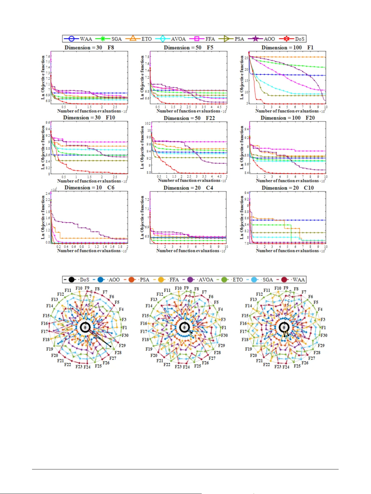
Dogﬁght Searc h: A Sw arm-Based Optimization Algor ithm f or Comple x Engineering Optimization and Mount ainous T er rain Path Planning Y ujing Sun a , Jie Cai a , Xingguo X u b , ∗ , Y uansheng Gao c , ∗ , Lei Zhang b , Kaichen Ouyang d and Zhan yu Liu b a Colleg e of Science, Liaoning T echnical U niver sity, F uxin, 123000, China b School of Mathematical Sciences, Dalian Univer sity of T ec hnology, Dalian, 116024, China c Colleg e of Com puter Science and T echnology, Zhejiang Univer sity, Hangzhou, 310027, China d Department of Physics, Univer sity of Science and T ec hnology of China, Hefei, 230026, China A R T I C L E I N F O Keyw ords : Optimization Metaheuristic Dogﬁght Search Engineering Optimization Mountainous T errain Path Planning A B S T R A C T Dogﬁght is a t actical behavior of cooperation between ﬁghters. Inspired by this, this paper pro- poses a novel metaphor-free metaheuristic algorit hm called Dogﬁght Search (DoS). Unlike tradi- tional algor ithms, DoS draw s algor ithmic framew ork from t he inspiration, but its search mecha- nism is constructed based on the displacement integration equations in kinematics. Through e x- perimental v alidation on CEC2017 and CEC2022 benchmark test functions, 10 real-w orld con- strained optimization problems and mountainous ter rain path planning tasks, DoS signiﬁcantl y outperforms 7 advanced competitors in ov erall performance and ranks ﬁrst in the Fr iedman rank - ing. Fur thermore, this paper compares t he performance of DoS with 3 SOT A algor ithms on the CEC2017 and CEC2022 benchmark test functions. The r esults show that DoS continues to maintain its lead, demonstrating strong competitiveness. The source code of DoS is av ailable at https://ww2.mathworks.cn/matlabcentral/ﬁlee xc hange/183519-dogﬁght-searc h. 1. Introduction Optimization problems are widel y present in various real-w orld domains, including engineer ing design ( Hao et al. , 2025 ), healt hcare ( Osaba et al. , 2019 ), logistics management ( Chu et al. , 2021 ) and ﬁnancial por tf olio opti- mization ( Dye , 2012 ). The quality of the obt ained solutions often directl y aﬀects sys tem per f ormance, resource alloca- tion eﬃciency , and economic beneﬁts. Therefore, designing eﬃcient and robust optimization algor ithms to obt ain the global optimal solution has become a core research direction in the ﬁeld of intelligent computing. Over the years, researchers ha ve proposed a series of tra- ditional optimization algor ithms, such as Ne wton ’ s method ( Su et al. , 2011 ) and gradient descent ( Hosseinali , 2024 ), based on t he linear characteristics of objective functions. These methods exhibit high computational eﬃciency and con ver gence accuracy in solving linear or con ve x optimiza- tion problems. Ho w ev er , their perf ormance is often lim- ited when dealing with complex real-w orld problems such as non-conv e xity or non-diﬀerentiability ( K eiv anian and Chiong , 2022 ; Deb et al. , 2002 ; Myers and Spencer , 2016 ; Gong et al. , 2010 ). Moreo v er , traditional algor ithms hea vil y rely on g radient information during iteration. As problem ∗ Corresponding author 2211060216@stu.lntu.edu.cn (Y . Sun); 2311010201@stu.lntu.edu.cn (J. Cai); xuxingguo@mail.dlut.edu.cn (X. Xu); y.gao@zju.edu.cn (Y . Gao); bhgleizhang@mail.dlut.edu.cn (L. Zhang); oykc@mail.ustc.edu.cn (K. Ouyang); ramirez@mail.dlut.edu.cn (Z. Liu) OR CID (s): 0009-0008-8286-7367 (X. Xu); 0000-0003-3278-8835 (Y . Gao) dimensionality increases, the complexity of gradient compu- tation also rises shar pl y , fur ther undermining their eﬃcie ncy in solving high-dimensional engineer ing problems. In contrast to the limitations of traditional methods, metaheuristic algor ithms ha ve shown greater adaptability and potential in complex optimization t asks due to t heir sim- ple implementation, low parameter dependency , and strong global search capabilities ( Dhiman and Kumar , 2019 ). For ex ample, Gholizadeh et al. proposed the Ne wton Meta- heuristic Algor ithm (NMA) ( Gholizadeh et al. , 2020 ) f or the seismic design of steel frame str uctures with discrete per- f ormance cr iteria, eﬀectivel y overcoming the limit ations of traditional methods in nonlinear and discrete design spaces. Houssein et al. de v eloped a h ybrid metaheur istic algorithm, BES-GO ( Houssein et al. , 2025 ), which demonstrated su- perior con v erg ence per f ormance and practical applicabil- ity in structural design benchmarks. In addition, Lu et al. introduced the Multi-Strategy Beetle Swarm Optimization (MBSO) ( Lu et al. , 2025 ) algorit hm to optimize air volume in mine ventilation networks, signiﬁcantly improving the energy eﬃciency of the system. These studies highlight the broad applicability and signiﬁcant de v elopment potential of metaheuristics in solving nonlinear, high-dimensional, and constrained engineering optimization problems. Represen- tative contributions are summarized in Table 1 . The core idea of metaheur is tic algor ithms is to build nature-inspired mathematical models and perform global search by simulating biological behaviors, physical phenom- ena, or natural law s. According to the No Free Lunch Theo- rem ( W olper t and Macready , 2002 ), no single algorithm can solv e all optimization problems optimally , which highlights Y ujing Sun et al.: Preprint submitted to Elsevier Page 1 of 56 Dogﬁght Sea rch T able 1 Contributions of metaheuristic algorithms to real-wo rld engineering problems. Algorithm Engineering Contribution Dual-Pheromone Crossov er Ant Colony Optimization (DPX- A CO) ( W ang et al. , 2025b ) The proposed method signiﬁcantly reduces the ov erall production costs in large-scale cotton blending optimization. Comprehensive experimental anal yses furt her demonstrate its eﬀectiveness, wit h sev eral benchmark scenar ios achie ving cost reductions ex ceeding 30%. Impro ved Discrete Particle Sw arm Optimization (IDPSO) ( W u et al. , 2025 ) Pro vided superior scheduling solutions f or automated guided vehicle manufacturing processes by consider ing dynamic c hanges, operator skills, and equipment maintenance, leading to a notable reduction in task completion time. Artiﬁcial Rabbits Optimization (ARO) ( Kuo et al. , 2025 ) Optimized control parameters of biped robots, enabling fast adaptation to external disturbances and maintaining balance in complex environments such as disaster response scenarios. Impro ved Ant Colony Optimization (IACO) ( W angying and Naiming , 2025 ) Applied to helicopter route planning f or forest ﬁre prevention, reducing total ﬂight distance by 4.1% and improving emergency response eﬃciency by 7.3% in dynamic en vironments. the importance of structural innovation tailored to speciﬁc problem characteristics. The performance of me taheur is tic algorithms largel y depends on t he balance between exploration and exploitation ( Arani et al. , 2013 ). How e ver , most e xisting algorithms ov erl y rely on the cur rent best solution as a guiding mech- anism. For instance, Particle Swarm Optimization (PSO), proposed by Kennedy et al. based on bird f oraging behav - ior ( Kennedy and Eberhar t , 1995 ); Grey W olf Optimizer (GW O), introduced b y Mirjalili et al. based on the c ooper a- tive hunting strategy of grey wolv es ( Mir jalili et al. , 2014 ); and Blac k Wing ed Kite Algorithm (BKA), pr oposed b y W ang et al. based on the aer ial hunting beha vior of blac k - winged kites ( W ang et al. , 2024 ). While these algor ithms perform well in speciﬁc applications, experimental results show that e x cessive dependence on the current best solution tends to reduce population diversity , leading to premature con ver gence ( Gao et al. , 2025b ). This br ings forth t he ﬁrst research question: How to design more reasonable guidance mechanisms to maint ain population diversity and eﬀectivel y a v oid local optima in comple x search spaces? On the o ther hand, man y metaheuristic algor ithms adopt only a single search strategy , making it diﬃcult to dynam- ically balance exploration and exploitation throughout the entire optimization process. For example, both PSO and the PID-based Search Algorit hm (PSA) proposed by Gao ( Gao , 2023 ) suﬀer from this limit ation. Although JADE, proposed by Zhang et al. ( Zhang and Sanderson , 2009 ), introduces dynamic parame ter adaptation to enhance searc h diversity , e xperiment al results still show that J ADE’ s pop- ulation div ersity remains limited. This leads to t he second research question: Ho w to achiev e a more eﬃcient balance betw een exploration and e xploitation through mu lti-s trategy collaboration and adaptiv e regulation mechanisms? In recent years, an increasing number of researchers ha ve dra wn attention to the phenomenon of o v er -metaphorization in metaheur is tic algor ithm design ( Sörensen , 2015 ). These algorit hms tend to rely heavil y on natural metaphors while ov erlooking the underlying mathematical pr inciples. Al- though such algorit hms ha ve achie v ed success in some en- gineering applications, their abstract nature and lac k of generalizability limit both extensibility and innovation po- tential ( Camacho- Villalón et al. , 2023 ). Therefor e, designing metaphor -free metaheur istic algor ithms with strong per f or - mance and practical value has become a ne w research trend. Sev eral studies hav e made progress in t his direction. For example, Logistic Gauss Circle Optimizer, proposed by W ang et al. ( W ang et al. , 2025a ), though inspired by three types of chaotic maps, essentially regulates exploration and exploitation through t he cooperative use of Logistic, Gauss, and Circle chaos mechanisms. Similarly , the Delta Plus algor ithm dev eloped by Gao et al. completely abandons metaphor -driven design and instead constr ucts an optimiza- tion framew ork based purely on t he general search principles of metaheur is tics, oﬀer ing a new perspectiv e for t he devel- opment of metaphor -free algorit hms. Based on the above motivations, we propose a metaphor - free metaheur istic algor ithm inspired by the dogﬁght beha v- ior of ﬁghter jets, called Dogﬁght Search (DoS). Diﬀerent from traditional algor ithms such as Genetic Algorit hm (GA) ( Holland , 1992 ) and PSO, DoS introduces a dual formation structure and distinguishes the solutions within the forma- tion as "leader aircraft" and "wing aircraft", where wing air- craft possess t he ability to dynamically select search strate- gies to achiev e adaptive adjustment between exploration and exploitation. In the search process, DoS incor porates the displacement integration equations from kinematics ( Zohar et al. , 2011 ), coordinating ﬁv e search strategies through the adjustment of direction vectors, ﬂight speed, and ﬂight time, thereby enhancing the ov erall algorithm per f ormance. Although the concept of DoS originates from the dogﬁght beha vior of ﬁghter jets, its search mechanism is detached from metaphors and it achie v es results super ior to SOT A algorit hms in CEC2017 and CEC2022 benchmark test func- tions. The main contributions of this paper are: (1) A metaphor -free metaheuristic algor ithm, named DoS, is proposed; Y ujing Sun et al.: Preprint submitted to Elsevier P age 2 of 56 Dogﬁght Sea rch (2) In CEC2017 (30, 50, 100 dimensions) and CEC2022 (10, 20 dimensions) benchmark test functions, DoS demonstrated signiﬁcantly superior per f ormance com- pared to sev en advanced competitors; Fur ther more, DoS achie v ed the top Friedman ranking when compared against three SOT A algor ithms: L SHADE ( T anabe and Fukunaga , 2014 ), LSHADE-SP A CMA ( Mohamed et al. , 2017 ) and AL -SHADE ( Li et al. , 2022 ), demon- strating strong competitiveness; (3) DoS ranks ﬁrst in ov erall per f ormance on real-world en- gineering optimization problems. It remains st atis tically superior in problems with 91 inequality constraints, conﬁrming its engineer ing applicability ; (4) In mountainous ter rain pat h planning t asks wit h and without no-ﬂy zones, DoS also demonstrates signiﬁ- cantly super ior performance compared to competitors. The rest of t his paper is organized as follo w s: Section 2 introduces related research on metaheur istic algor ithms; Section 3 descr ibes the design inspiration and mathematical model of DoS; Section 4 evaluates DoS numerically on multidimensional CEC2017 and CEC2022 benchmark test functions; Section 5 veriﬁes the per f ormance of DoS on solving constrained optimization problems through various real-w orld tasks; Section 6 fur ther validates the advantages of DoS in solving mountainous ter rain path planning prob- lems; Section 7 discusses the advantages and limit ations of DoS; Section 8 summar izes t he wor k and points out potential future research directions based on DoS. 2. Related studies The classiﬁcation of metaheur is tic algor ithms is mainly reﬂected in two aspects. As shown in Fig. 1 , based on the number of solutions, algor ithms can be categorized into two major types: single-solution-based algorithms and multi- solution-based algorit hms. The classiﬁcation of single-solution-based algor ithms lies in their search process relying on a single-solution. A representative example is the Simulated Annealing (S A) proposed by Kirkpatrick et al. in 1983 ( Kirkpatr ic k et al. , 1983 ), which w as inspired by the energy changes in the cooling pr ocess of solids. Due to t he limited global in- f ormation obtained from a single-solution, S A introduces a probability mechanism for accepting worse solutions to escape local optima and enhance exploration ability . Other representative algorit hms include the T abu Search Algo- rit hm (TS A) ( Prajapati et al. , 2020 ), Random Search (RS) ( Zabinsky et al. , 2009 ) and Non-monopolize Search (NO) ( Abualigah et al. , 2024 ). Although this type of algor ithm has advantages in conv erg ence speed, its low information utiliza- tion eﬃciency often makes it diﬃcult to deal wit h complex high dimensional problems, whic h in turn has promoted the dev elopment of multi-solution-based algorithms. Multi-solution-based algor ithms utilize information from multiple solutions to guide the search, t hereb y enhancing global search ability . Although t he design inspirations of such methods are diverse, including animal beha viors, natu- ral phenomena, physical law s and mathematical functions, their classiﬁcation depends on the search mechanisms. Multi-solution-based algorit hms can be fur ther categorized into ev olution-based algor ithms and sw arm-based algo- rit hms ( Ezugwu et al. , 2021 ). Ev olution-based algor ithms are based on Darwin’ s t he- ory of ev olution and stress gene tic crossov er and mu tation operations on decision variables throughout the optimization process. A typical representative is the Genetic Algor ithm (GA) proposed by Forrest et al., which continuously op- timizes candidate solutions through mechanisms such as selection, crosso ver and mutation. Other ev olutionary ap- proaches include Diﬀerential Ev olution (DE) ( S torn and Price , 1997 ), Genetic Programming (GP) ( Koza , 1994 ) and Lov e Ev olution Algorithm (LEA) ( Gao et al. , 2024 ). Sw arm-based algor ithms form t he larg est subclass, dra w- ing inspiration from biological beha viors, physical pro- cesses, and mathematical models. Among t hem, typical algorit hms inspired b y biological activities include PSO and Ant Colony Optimization (ACO) ( Dor igo , 1991 ). The latter was proposed by Dor igo in 1991 and simulates the pheromone mechanism of ants for optimization. A repre- sentative of phy sics inspired algor ithms is the Gravitational Search Algor ithm (GSA) ( Rashedi et al. , 2009 ), which simulates gravitational interactions between solutions to achie v e global guidance. Mathematics inspired algorit hms include the Sine Cosine Algorithm (SCA) ( Mirjalili , 2016 ), which lever ages the periodicity of tr igonometric functions to enhance search div ersity . In addition to the abov e typical methods, swarm-based algor ithms also include: Beav er Be- ha vior Optimizer (BBO) ( Ouyang et al. , 2025 ), Philoponella Prominens Optimizer (PPO) ( Gao et al. , 2025a ), Escape Al- gorit hm (ESC) ( Ouy ang e t al. , 2024 ), T raﬃc Jam Optimizer (TJO) ( W ang and Shang , 2025 ), Multi- V erse Optimizer (MV O) ( Mirjalili et al. , 2016 ), Atom Search Optimization (ASO) ( Zhao e t al. , 2019 ) and W eighted A verage Algor ithm (W AA) ( Cheng and De W aele , 2024 ). Although these algor ithms per f orm well in various prob- lems, most swarm-based algorit hms share two common shortcomings. First, the guidance information o ver ly de- pends on the population ’ s best solution and lacks div ersiﬁed guidance, making the search pr one to local optima. Second, the number of search strategies is usually no more than three, resulting in monotonous search beha vior . These limit ations reduce their search eﬃciency in comple x f easible regions. T o address the abov e issues, t he proposed DoS intro- duces multiple guiding solutions in its design to enhance diversity . In addition, DoS assigns wing aircrafts a dynamic search strategy selection mec hanism to eﬀectiv ely balance exploration and exploitation. 3. Methodology This section will introduce the design inspiration, math- ematical model, pseudocode and theoretical analy sis of t he computational complexity of DoS. Y ujing Sun et al.: Preprint submitted to Elsevier P age 3 of 56 Dogﬁght Sea rch Mul ti - Sol ution - Bas ed Alg ori th m s SA TS A RS NO DE GA ACO LEA GP Evolut i on - B ased A lgor ithms S wa r m - B a se d Algor it hms MVO ES C TJO S C A P P O G SA PS O B B O ASO W A A Sin gle - Sol ution - B ased Algor it hms Me t a h e u ri s ti c s Mul ti - Sol ution - Bas ed Alg ori th m s SA TS A RS NO DE GA ACO LEA GP Evolut i on - B ased A lgor ithms S wa r m - B a se d Algor it hms MVO ES C TJO S C A P P O G SA PS O B B O ASO W A A Sin gle - Sol ution - B ased Algor it hms Me t a h e u ri s ti c s Figure 1: The classiﬁcation of metaheuristic algorithms. 3.1. Inspiration Dogﬁghting ( Ashraf et al. , 2021 ) is a highly dynamic air combat behavior , which is typically divided into two phases: attack and ev asion. In the att ac k phase, ﬁghter jets car ry out strikes b y chasing and locking onto enemy aircraft and launching missiles. In the evasion phase, they rely on ir regular and chaotic ﬂight trajectories to escape enemy lock - on and missile tracking ( Greenw ood , 1992 ). T wo ﬁghter jet f ormations strive to achie v e the best combat readiness through adjustments to t heir positions and combat strategies, thereby securing victor y . This process bears a str iking re- semblance to the optimization solutions employ ed in meta- heuristic algor ithms. This process is highly similar to t he optimization solving process in metaheuristic algor ithms. Theref ore, inspired by this beha vior , we designed ﬁv e types of search strategies for DoS: free ﬂight, maneuv er lock - on, missile attack, maneuver ev asion and ﬂare ev asion. To better e xplain the algor ithm design concept, we abstract the inspirations as f ollo ws: (1) Solution: the position of a ﬁghter jet. W e divide the ﬁghter g roup into two formations, which are adversarial to each o ther; (2) Feasible domain: the airspace in which t he ﬁghter jets conduct their search; (3) Function value: t he combat state of the ﬁghter jet. For minimization problems, the better the combat state, t he smaller the function value; (4) Global optimal solution: the location in the airspace wit h the best combat state. Fig. 2 (a) show s the inspiration source of t he free ﬂight strategy in DoS ( Olsder and Breakwell , 1974 ). In this strat- egy , the leader aircraf t and wing aircraf t randomly search the airspace based on commands from the command center , while the wing aircraft continuousl y cooperates with the leader aircraft, enabling eﬃcient exploration of the airspace. Fig. 2 (b) and (c) illus trate the maneuv er lock -on and missile attack strategies, respectiv ely . Both strategies focus on en- emy aircraft as core t ar ge ts and exhibit strong conv er gence and guidance, promoting local exploitation and improving solution accuracy . Fig. 2 (d) and (e) illustrate the maneuver ev asion and ﬂare evasion strategies. In t his phase, ﬁghter jets rapidly disengage from the cur rent airspace and mov e tow ard new ﬂight regions to av oid threats. From the perspective of search behavior , this process show s clear global explo- ration capability . The synergy of these ﬁve strategies enables the solutions to continuously mov e tow ard better regions, thereby impro ving o v erall search eﬃciency . It is impor tant to emphasize that alt hough DoS is in- spired by dogﬁghting beha vior, its search strategies are mathematically modeled based on the displacement inte- gration equations in kinematics. Speciﬁcall y , we conduct diversiﬁed modeling of key elements such as the direction vect or, ﬂight speed and ﬂight duration in DoS, thereby achie ving metaphor -free search operations. 3.2. Mathematical model of the search strategy The w orkﬂo w of DoS is shown in Fig. 3 , which sequen- tially includes initialization (see Section 3.2.1), the calcu- lation of the number of leader aircrafts and the inﬂuencing f actors of search strategies (see Sections 3.2.1 and 3.2.2), the search strategies of the tw o formations (see Sections 3.2.2 to 3.2.4) and the dynamic selection mechanism of wing aircraf t (see Section 3.3). T o facilitate understanding of the dual formation de- sign in DoS, Section 3.2.1 ﬁrst introduces the constr uction of the dual f ormation and the method f or calculating t he number of leader aircrafts in each iteration; Section 3.2.1 also explains the initialization strategy t ailored to the dual Y ujing Sun et al.: Preprint submitted to Elsevier P age 4 of 56 Dogﬁght Sea rch (a) Free ﬂight strategy (b) Maneuver lock -on strategy (c) Missile attack strategy (d) Maneuver evasion strategy (e) Flare ev asion strategy Figure 2: The inspiration diagram of DoS search strategies. f ormation design of DoS. Consider ing that the ﬁve types of searc h strategies f ollo w the same fundamental principles, Section 3.2.2 pro vides a uniﬁed e xplanation of the common principles behind these strategies, including the mathemati- cal meanings of ke y f actors such as direction vector , ﬂight speed and ﬂight duration. Subsequently , Sections 3.2.3 to 3.2.5 respectivel y present the speciﬁc settings of the relev ant parameters in the ﬁv e search s trategies. 3.2.1. Initialization of Dual F ormations T o meet t he requirements of t he dual formation structure in DoS, we assume that the total number of formation solu- tions ( 𝑁 ) is an ev en number . Among them, 𝑁 ∕2 solutions are deﬁned as the stealth ﬁghter f ormation ( 𝑿 ) and the remaining 𝑁 ∕2 solutions are deﬁned as the regular ﬁghter f ormation ( 𝒀 ). T o av oid con v erg ence to local optima caused by rel ying on a single guiding solution, leader aircrafts ser v e as the guiding solutions and wing aircraf ts adopt search strategies through a dynamic selection mechanism. Fur thermore, to broaden the exploration rang e of the formation, t he number of leader aircrafts is randomly selected within a deﬁned interval, as expressed in Equation 1 . 𝑝 = round  𝑘 1 +  1 2 − 𝑘 1  − 𝑟 1  − 𝑁 2  (1) where 𝑝 denotes the number of leader aircrafts, 𝑘 1 is a tunable hyperparameter in DoS and 𝑟 1 is a random number unif ormly distributed in t he inter v al [0 , 1] . It can be seen Y ujing Sun et al.: Preprint submitted to Elsevier P age 5 of 56 Dogﬁght Sea rch S tar t t < = T E n d C alcul ate t he fun cti on val ue of t he upda te d s olut ion and upda t e the va lua bl e sol uti on matr ix t = t + 1 Upda t e the inde x of the so l ut i ons wit hi n t he swa r m S t e a lt h fighter swa rm (1) Ge ne ra t e the numbe r of lea d a irc r a ft; (2) Obta in t he mi nim um flight spe e d; (3) Obta in t he ma xi mum flight spe e d; (4) Obta in t he a c c e ler a ti on; (5) S e t i = 1 (1) Ge ne ra t e the numbe r of lea d a irc r a ft; (2) Obta in t he mi nim um flight spe e d; (3) Obta in t he ma xi mum flight spe e d; (4) Obta in t he a c c e ler a ti on; (5) S e t i = 1 i <= N Upda t e the solut ion a c c or ding to A lgor ithm 1 Upda t e the solut ion a c c ording to Algorithm 3 i < = p i = i + 1 Ye s No Ye s No R e gula r fighte r s w a rm (1) Ge ne ra t e the numbe r of lea d a irc r a ft; (2) Obta in t he mi nim um flight spe e d; (3) Obta in t he ma xi mum flight spe e d; (4) Obta in t he a c c e ler a ti on; (5) S e t i = 1 (1) Ge ne ra t e the numbe r of lea d a irc r a ft; (2) Obta in t he mi nim um flight spe e d; (3) Obta in t he ma xi mum flight spe e d; (4) Obta in t he a c c e ler a ti on; (5) S e t i = 1 i < = N Upda t e the solut ion a c c ording to Algorithm 2 Upda t e the solut ion a c c ording to Algorithm 3 i < = p i = i + 1 Ye s No Ye s No (1) Initiali z e a ll sol uti ons wit hin t he swa rm ; (2) C a lcula te t he func ti on va lue s o f a ll solut ions; ( 3) Ca lc ula te t he inde x of the solutions withi n t he swa r m ; (4) Initiali z e the va luable sol uti on matr ix ; (5) S e t t = 0 (1) Initiali z e a ll sol uti ons wit hin t he swa rm ; (2) C a lcula te t he func ti on va lue s o f a ll solut ions; ( 3) Ca lc ula te t he inde x of the solutions withi n t he swa r m ; (4) Initiali z e the va luable sol uti on matr ix ; (5) S e t t = 0 Ye s No S tar t t < = T E n d C alcul ate t he fun cti on val ue of t he upda te d s olut ion and upda t e the va lua bl e sol uti on matr ix t = t + 1 Upda t e the inde x of the so l ut i ons wit hi n t he swa r m S t e a lt h fighter swa rm (1) Ge ne ra t e the numbe r of lea d a irc r a ft; (2) Obta in t he mi nim um flight spe e d; (3) Obta in t he ma xi mum flight spe e d; (4) Obta in t he a c c e ler a ti on; (5) S e t i = 1 i <= N Upda t e the solut ion a c c or ding to A lgor ithm 1 Upda t e the solut ion a c c ording to Algorithm 3 i < = p i = i + 1 Ye s No Ye s No R e gula r fighte r s w a rm (1) Ge ne ra t e the numbe r of lea d a irc r a ft; (2) Obta in t he mi nim um flight spe e d; (3) Obta in t he ma xi mum flight spe e d; (4) Obta in t he a c c e ler a ti on; (5) S e t i = 1 i < = N Upda t e the solut ion a c c ording to Algorithm 2 Upda t e the solut ion a c c ording to Algorithm 3 i < = p i = i + 1 Ye s No Ye s No (1) Initiali z e a ll sol uti ons wit hin t he swa rm ; (2) C a lcula te t he func ti on va lue s o f a ll solut ions; ( 3) Ca lc ula te t he inde x of the solutions withi n t he swa r m ; (4) Initiali z e the va luable sol uti on matr ix ; (5) S e t t = 0 Ye s No Figure 3: The iterative ﬂo wcha rt of DoS. that t he number of leader aircraf ts is constrained wit hin the range [ 𝑘 1 𝑁 , 0 . 25 𝑁 ] , which not only expands t he exploration radius of t he formation but also reser v es a suﬃcient propor - tion of wing aircrafts to better achie v e a balance between exploration and exploitation. Considering that DoS adopts a dual f ormation str ucture and integrates multiple searc h strategies, more dispersed initial formations yield more eﬀectiv e searches. Theref ore, this paper proposes an initialization strategy diﬀerent from traditional methods, whose f orm is shown in Eq uation 2 . 𝑿 𝑖𝑗 = 𝑳 𝑗 +  𝑼 𝑗 + 𝑳 𝑗 2 − 𝑳 𝑗  𝑟 2 , 𝒀 𝑖𝑗 = 𝑼 𝑗 + 𝑳 𝑗 2 +  𝑼 𝑗 − 𝑼 𝑗 + 𝑳 𝑗 2  𝑟 2 , 𝑖 = 1 , 2 , … , 𝑁 ∕2 , 𝑗 = 1 , 2 , … , 𝐷 (2) where 𝑿 represents the stealth ﬁghter formation, 𝒀 repre- sents t he regular ﬁghter formation, 𝑼 and L are the upper and low er bound vectors of the decision variables, 𝐷 is t he problem dimension and 𝑟 2 is a random number uniformly distributed wit hin [0 , 1] . This initialization strategy divides the f easible domain into tw o sub inter v als, upper and low er Y ujing Sun et al.: Preprint submitted to Elsevier P age 6 of 56 Dogﬁght Sea rch based on the hyperplane formed by the midpoints of each dimension ( Winder , 1966 ), which are then used as the ini- tialization ranges f or the stealth ﬁghter formation and t he regular ﬁghter f ormation, respectivel y . By placing the two formations in spatially distinct re- gions based on this domain par titioning, the strategy en- hances the spread of solutions in t he earl y search stage. This spatial separation also suppor ts the subsequent att ac k and ev asion strategies, thereby improving t he exploration eﬃciency of DoS. 3.2.2. Common Pr inciples of Search Strategies Although DoS uses dogﬁghting beha vior as an exter - nal expression, the mathematical models of the 5 search strategies are based on the kinematics and displacement integration equations sho wn in Equation 3 . 𝑋 𝑖 𝑛𝑒𝑤 = 𝑋 𝑖 + ∫ Δ 𝜉 0 𝒖 ⋅ 𝑣 𝑑 𝜉 , 𝑖 = 1 , 2 , … , 𝑁 ∕2 (3) where 𝒖 denotes t he direction vector , v denotes the ﬂight speed and represents the ﬂight duration. Since DoS sorts the solutions within eac h formation in ascending order based on their function v alues at t he end of each iteration, solutions with better function values are ranked earlier . The top p solutions are deﬁned as leader aircrafts and the remaining solutions are deﬁned as wing aircraf ts. In Sections 3.2.2 to 3.2.4, based on t he distinction between leader aircrafts and wing aircrafts, the direction vector u is fur ther divided into 𝒖 𝒍𝒆𝒂𝒅 𝒆𝒓 and 𝒖 𝒘𝒊𝒏𝒈 . As sho wn in Equation 3 , regardless of which search strategy is adopted, the update of a solution depends on three ke y factors: u, v and . This paper lev erages diﬀerentiated deﬁnitions of these t hree factors to implement the eﬀects of the ﬁve searc h strategies. Decomposition of the dir ection vect or: In most metaheur is tic algor ithms, a solution ’ s direction is typically determined b y intraf ormation inf ormation alone. As a result, it is of ten diﬃcult to escape local optima when solving comple x optimization problems. T o address this, DoS decomposes 𝑢 into two components: pilot guidance ( 𝒖 𝐏𝐢𝐥𝐨𝐭 ) and command guidance ( 𝒖 𝐇𝐞𝐚𝐝 ). Speciﬁcally : (1) 𝒖 𝐏𝐢𝐥𝐨𝐭 : t he direction vector determined by intra-formation pilot inf ormation; (2) 𝒖 𝐇𝐞𝐚𝐝 : t he direction vector determined by informativ e and high-quality solutions. Theref ore, uHead helps solutions escape from local op- tima in a timely manner and explore new potential regions. Since uPilot must be designed to meet t he exploration and exploitation needs of diﬀerent strategies, its deﬁnition is elaborated in Sections 3.2.2 to 3.2.4. The mathematical form of uHead is shown in Equation 4 . 𝑅 1 = r ound( 𝑁 𝑅 ⋅ 𝑟 3 ) , 𝑅 2 = r ound( 𝑁 𝑃 ⋅ 𝑟 4 ) , 𝒖 𝐇𝐞𝐚𝐝 = 𝑿 𝑅 1 − 𝒁 𝑅 2 (4) where 𝑅 1 denotes t he index of a randomly selected high- quality solution, 𝑁 𝑅 denotes the number of high quality solutions (ﬁxed at 0 . 1 𝑁 ), 𝑍 is the storage matr ix of valuable solutions, 𝑅 2 denotes the inde x of a randoml y selected v alu- able solution, 𝑁 𝑃 denotes t he number of stored valuable solutions (with a maximum of 2 . 5 𝑁 ) and 𝑟 3 and 𝑟 4 are random numbers unif ormly distributed in the range [0 , 1] . Minimum speed, maximum speed and acceleration: In DoS, t he motion state of solution updates is modeled as either uniform or uniformly accelerated motion. There- f ore, 𝑣 is de ter mined by three inﬂuencing f actors: minimum speed ( 𝑣 𝑚𝑖𝑛 ), maximum speed ( 𝑣 𝑚𝑎𝑥 ) and acceleration ( 𝑎 ). As shown in Equation 3 , 𝑣 is closely related to the step size of solution updates. If speed can be appropr iatel y q uantiﬁed to guide the update of solutions tow ard positions with low er function values, the search eﬃciency can be signiﬁcantly impro ved. To achiev e this, DoS records promising solu- tions (i.e., those with decreasing function values) at the end of each iteration and uses the v elocity and function value information of these promising solutions to update the initial velocity f or the next iteration. Details are shown in Equation 5 . 𝑉 𝑛𝑒𝑤 =  𝑖 ∈Ω 𝑾 𝑖 ⋅ 𝑽 2 𝑖  𝑖 ∈Ω 𝑾 𝑖 ⋅ 𝑽 𝑖 , 𝑾 𝑖 = 𝑑 𝒇 𝑖     𝑖 ∈Ω 𝑑 𝒇 𝑗    (5) where 𝑉 𝑛𝑒𝑤 denotes the initial velocity f or the next iteration, Ω represents the set of indices of promising solutions, 𝑽 𝑖 and 𝑑 𝒇 𝑖 denote t he ﬂight velocity and function value diﬀerence of the 𝑖 -th promising solution, respectivel y . To enhance so- lution div ersity , DoS adds real-v alued random per turbations to the initial velocity , as shown in Eq uation 6 . 𝑉 = 𝑉 𝑛𝑒𝑤 + t an  𝜋 2 ( 𝑟 5 − 0 . 5)  ∕10 (6) where 𝑟 5 is a random number uniformly distributed in the range [0 , 1] and the velocity 𝑉 obt ained from Equation 6 can be further used to deﬁne the minimum speed, maximum speed and acceleration of a solution in the next iteration, as shown in Equation 7 . 𝑣 min = min{ 𝑘 5 𝑉 , 𝑉 } , 𝑣 max = max{ 𝑘 5 𝑉 , 𝑉 } , 𝑎 = ( 𝑣 max − 𝑣 min )∕1 . 2 (7) where 𝑘 5 is a tunable hyperparameter in DoS and belongs to the inter v al [0 , 1] . Flight duration : In Equation 3 , Δ 𝜉 is also a key f actor shaping the solution ’ s update radius. Since 𝑣 has already achiev ed suf- ﬁcient diversiﬁcation of the mo v ement radius, this paper Δ 𝜉 designs as a control factor f or diversiﬁed search regions, allowing solutions to be updated within a certain range. The speciﬁc f ormulation is shown in Equation 8 . Δ 𝜉 = 0 . 8 + 0 . 4 𝑟 6 (8) where 𝑟 6 is a random number uniformly distributed in the range [0 , 1] and thus is a uniformly distributed random value within t he inter val [0 . 8 , 1 . 2] . This setting allows solutions to perform ﬁne grained exploitation within a small range while also expanding t he exploration radius ov er a larger range, thereby impro ving o v erall search eﬃciency . Y ujing Sun et al.: Preprint submitted to Elsevier P age 7 of 56 Dogﬁght Sea rch 3.2.3. F ree Flight Strategy In t his subsection and the subsequent descriptions of the mathematical models f or search strategies, we f ocus on the design of the direction vector and ﬂight speed. It is import ant to note that, to improv e the search eﬃciency of DoS in the earl y iterations, the two formations diﬀer only in the strategy selection mechanism dur ing the earl y stage (see Section 3.3), while t heir mathematical expressions remain identical. Theref ore, t his paper uses the stealth ﬁghter f ormation as t he uniﬁed ex ample f or e xplanation. In the early stage of iteration, due to the lack of pr ior know ledg e about the solution space of the optimization problem, it is necessary to conduct global exploration of the f easible domain. As information about the solution space accumulates, a g radual balance betw een exploration and exploitation should be achie ved. Based on t his, a “free ﬂight” strategy is designed for DoS. Under this strategy , the direction vectors of leader aircrafts and wing aircrafts are deﬁned as f ollow s, as sho wn in Equation 9 . 𝒖 𝐏𝐢𝐥𝐨𝐭 𝐥𝐞𝐚𝐝𝐞𝐫 = 𝑿 𝒓𝒂𝒏𝒅 − 𝑿 𝑖 , 𝒖 𝐏𝐢𝐥𝐨𝐭 𝐰𝐢𝐧𝐠 = 𝑿 𝐻 − 𝑿 𝑖 , 𝑿 𝒓𝒂𝒏𝒅 = 𝑳 + ( 𝑼 − 𝑳 ) 𝑟 7 (9) where leader denotes the leader aircraf t, wing denotes t he wing aircraf t, 𝐻 indicates the index of the leader aircraft f ollow ed by the wing aircraft and 𝑟 7 is a random number uni- f ormly distr ibuted in t he range [0 , 1] . Under t his mechanism, leader aircraf ts conduct random exploration within the feasi- ble domain, while wing aircrafts per f orm local e xploitation along t he ﬂight path of leader aircrafts, thereb y signiﬁcantl y impro ving the discov ery eﬃciency of high-quality solutions during t he early stages of iteration. Since an excessiv el y large step size may cause the update process to miss some valuable solutions, the motion state under this strategy is modeled as uniform motion with a speed of 𝑣 𝑚𝑖𝑛 . By incor porating the ﬂight duration deﬁned in Eq uation 8 and substituting it into Equation 3 , the mathe- matical model of the free ﬂight strategy is obtained, as shown in Equation 10 .  𝑿 𝑖 𝒏𝒆𝒘 = 𝑿 𝑖 +  𝒖 𝐏𝐢𝐥𝐨𝐭 𝐥𝐞𝐚𝐝𝐞𝐫 + 𝒖 𝐇𝐞𝐚𝐝  𝑣 min ⋅ Δ 𝜉 , 𝑖 ≤ 𝑝 𝑿 𝑖 𝒏𝒆𝒘 = 𝑿 𝑖 +  𝒖 𝐏𝐢𝐥𝐨𝐭 𝐰𝐢𝐧𝐠 + 𝒖 𝐇𝐞𝐚𝐝  𝑣 min ⋅ Δ 𝜉 , 𝑖 > 𝑝 (10) where 𝑿 𝑖 𝒏𝒆𝒘 denotes t he updated position of t he 𝑖 -th leader aircraft or wing aircraf t. To intuitivel y demonstrate the beha vioral characteristics of this str ategy , it is visualized in a tw o dimensional plane, as shown in Fig 4 . 3.2.4. Oﬀensive Strategy Although t he free ﬂight strategy can achiev e a dy- namic balance betw een exploration and exploitation in the earl y st ag es of iteration, relying on a single search strat- egy throughout the entire iteration process will inevitably limit the diversity of search beha vior . T o address this, two oﬀensive strategies are designed f or DoS to enhance its local exploitation ability around valuable solutions. These strategies are inspired b y the processes of pursuing and locking onto enemy aircraft, as well as missile attacks during dogﬁghts and are t hus named the maneuver loc k -on and missile attack strategies. The mathematical models of these strategies are described below . Maneuver lock -on strategy: Most metaheur istic algor ithms rely on a single popula- tion, which makes them prone to f alling into local optima, resulting in many iterations without meaningful improv e- ment. Sudholt ( Sudholt , 2019 ) pointed out that increasing the number of populations can improv e search diversity . Based on t his, DoS lev erag es the advantages of its dual f or - mation str ucture, allo wing both oﬀensive strategies to obtain exploitation inf ormation from the opposing formation. The computation function f or the pilot guided direction vector in the maneuver loc k -on strategy is shown in Eq uation 11 . 𝒖 𝐏𝐢𝐥𝐨𝐭 𝟏 = 𝒀 ℎ − 𝑿 𝑖 , 𝒖 𝐏𝐢𝐥𝐨𝐭 𝟐 = 𝒀 ℎ 𝒑𝒓𝒆 − 𝑿 𝑖 , 𝒖 𝐏𝐢𝐥𝐨𝐭 = 𝑟 8 ⋅ 𝒖 𝐏𝐢𝐥𝐨𝐭 𝟏 + (1 − 𝑟 8 ) 𝒖 𝐏𝐢𝐥𝐨𝐭 𝟐 (11) where 𝒀 denotes the coordinate matr ix of t he regular ﬁghter f ormation, ℎ is the inde x of the selected regular ﬁghter , 𝒀 ℎ 𝒑𝒓𝒆 represents the predicted position and 𝑟 8 is a random number unif ormly distributed in the range [0 , 1] . According to the equation, t he 𝒖 𝐏𝐢𝐥𝐨𝐭 under the maneuv er lock -on strategy is no longer distinguished between leader aircraft and wing aircraft. Instead, it is determined by tw o sub v ectors: (1) 𝒖 𝐏𝐢𝐥𝐨𝐭 𝟏 : determined based on the solution inf ormation from the opposing f ormation; (2) 𝒖 𝐏𝐢𝐥𝐨𝐭 𝟐 : deter mined based on both t he opposing formation and the best solution inf ormation, wit h the deﬁnition of 𝒀 ℎ 𝒑𝒓𝒆 given in Equation 12 . 𝒀 ℎ 𝒑𝒓𝒆 = 𝒀 ℎ +  𝒀 𝒃𝒆𝒔𝒕 − 𝒀 ℎ  𝑟 9 , ℎ ≤ 𝑝 (12) where 𝑟 9 is a random number uniformly distributed in the interval [0 , 1] and both 𝒀 ℎ and 𝒀 𝒃𝒆𝒔𝒕 are leader aircraft within the regular ﬁghter f ormation. The linear combination of these two yields 𝒀 ℎ 𝒑𝒓𝒆 , which possesses high exploitation value. Since 𝒀 ℎ 𝒑𝒓𝒆 does not belong to the opposing f orma- tion, this design ensures exploitation while also eﬀectivel y prev enting the two formations from conv erging prematurely . T o enr ic h the distribution div ersity of solutions after ex ecuting t he maneuver loc k -on strategy , t he motion state is modeled as uniformly accelerated motion. The cor respond- ing function describing velocity as a function of time is given in Equation 13 . 𝑣 𝜉 = 𝑣 min + 𝑎 ⋅ 𝜉 (13) By combining Equations 11 , 13 , 8 and 3 , the complete mathematical formulation of the maneuver loc k -on strategy can be derived, as sho wn in Equation 14 . 𝑿 𝑖 𝒏𝒆𝒘 = 𝑿 𝑖 + ∫ Δ 𝜉 0  𝒖 𝐏𝐢𝐥𝐨𝐭 + 𝒖 𝐇𝐞𝐚𝐝  𝑣 𝜉 ⋅ 𝑑 𝜉 = 𝑿 𝑖 +  𝒖 𝐏𝐢𝐥𝐨𝐭 + 𝒖 𝐇𝐞𝐚𝐝   𝑣 min + 1 2 𝑎 ⋅ Δ 𝜉 2  , 𝑖 = 1 , 2 , … , 𝑁 2 (14) Y ujing Sun et al.: Preprint submitted to Elsevier P age 8 of 56 Dogﬁght Sea rch ran d X le ad e r n e w X P il ot le ad e r u He ad u ( ) m i n v  +    P i l ot H e ad l e ad e r uu ( ) H le ade r XX P il ot w in g u ( ) m in v  +    P ilot He ad w in g uu w in g n e w X He ad u w in g X ran d X le ad e r n e w X P il ot le ad e r u He ad u ( ) m i n v  +    P i l ot H e ad l e ad e r uu ( ) H le ade r XX P il ot w in g u ( ) m in v  +    P ilot He ad w in g uu w in g n e w X He ad u w in g X Figure 4: Visualization of the free ﬂight strategy . h pre Y n e w X ( ) 2 m in 1 2 va   +  +     P ilot He ad uu He ad u h Y P il ot 1 u X P il ot 2 u P il ot u h pre Y n e w X ( ) 2 m in 1 2 va   +  +     P ilot He ad uu He ad u h Y P il ot 1 u X P il ot 2 u P il ot u Figure 5: Visualization of the maneuver lo cking strategy . T o intuitiv ely demonstrate the search behavior of this strategy , t he solution update process is visualized in a 2 dimensional space, as shown in Fig. 5 . Missile attack strategy : Although the maneuv er loc k -on strategy can pre vent the two f ormations from conv er ging prematurely , the algo- rit hm’ s reliance on exploitation does not completel y elimi- nate potential r isks. When t he solution approaches t he region containing the global optimal solution, if DoS relies solely on the maneuv er loc k -on strategy f or e xploitation, it ma y be misled by attractive local optima and f ail to fur ther explore the global optimal solution region. To address t his limitation, a missile attac k strategy is proposed in this paper . This strategy relies ex clusiv ely on information from t he opposing f ormation. The deﬁnition of 𝒖 𝐏𝐢𝐥𝐨𝐭 under this s trategy is pro vided in Equation 15 . 𝒖 𝐏𝐢𝐥𝐨𝐭 = 𝒀 ℎ − 𝑿 𝑖 , ℎ ≤ 𝑝 (15) Although this setting may cause the two f ormations to conv erg e prematurely to t he same solution region, t he ex ecution frequency of t his strategy has been appropr iatel y reduced within the iterativ e process of DoS. As long as the majority of solutions still adopt the maneuver lock -on strategy , t his issue can be eﬀectivel y a voided. Since the missile attack strategy requires solutions to mov e aw a y from their original regions and g raduall y ap- proach the global optimal, the motion state under this strat- egy is modeled as unif ormly decelerated motion. The corre- sponding velocity function is given in Equation 16 . 𝑣 𝜉 = 𝑣 max − 𝑎 ⋅ 𝜉 (16) By combining Equations 15 , 16 , 8 and 3 , the complete mathematical f ormulation of the missile att ac k strategy can be derived, as sho wn in Equation 17 . 𝑿 𝑖 𝒏𝒆𝒘 = 𝑿 𝑖 + ∫ Δ 𝜉 0  𝒖 𝐏𝐢𝐥𝐨𝐭 + 𝒖 𝐇𝐞𝐚𝐝  𝑣 𝜉 ⋅ 𝑑 𝜉 = 𝑿 𝑖 +  𝒖 𝐏𝐢𝐥𝐨𝐭 + 𝒖 𝐇𝐞𝐚𝐝   𝑣 max − 1 2 𝑎 ⋅ Δ 𝜉 2  , 𝑖 = 1 , 2 , … , 𝑁 2 (17) In summar y , t he exploitation mechanism of DoS inte- grates both the maneuver loc k -on and missile attack strate- gies: t he f ormer utilizes high quality inf ormation bey ond Y ujing Sun et al.: Preprint submitted to Elsevier P age 9 of 56 Dogﬁght Sea rch the opposing formation to achiev e eﬃcient exploitation and a v oid con ver gence consistency , while the latter ensures deep exploration of the global optimal solution. Their synergy allow s DoS to maint ain exploitation diversity while improv e global performance. 3.2.5. Evasiv e Strategy The oﬀensive strategies proposed in Section 3.2.4 ha v e already satisﬁed t he exploitation requirements of DoS; ho w - ev er , exploration is also a cr itical factor throughout diﬀerent stages of iteration. If explor ation is insuﬃcient in t he early stage, the eﬃciency of gather ing inf ormation about the so- lution space will be low ; if it is insuﬃcient in the middle and later stages, the algorit hm is prone to g etting trapped in local optima and may fail to conv erg e to the global optimal solution. To address the exploration needs in the early stage, the free ﬂight strategy has been designed. For the middle and later stages, in order to furt her enhance the exploration capability of DoS, two ev asion strategies are proposed, namely t he maneuv er ev asion and ﬂare ev asion strategies. These strategies are inspired by the ev asiv e maneuvers and ﬂare release beha viors of ﬁghter jets during dogﬁghts. Maneuver evasion strat egy: In the middle and later stages of iteration, the main role of e xploration strategies is t o help solutions escape local optima. Therefor e, 𝒖 𝐏𝐢𝐥𝐨𝐭 should be decoupled from the cur rent exploitation region and reor iented within t he feasible domain. Howe v er, if completely random search, as in the free ﬂight strategy , is adopted again, the optimization accuracy ma y be sever ely degraded. T o a v oid t his, the mathematical model of 𝒖 𝐏𝐢𝐥𝐨𝐭 in t his paper is based on t he set of stored valuable solutions, as deﬁned in Equation 18 . 𝒖 𝐏𝐢𝐥𝐨𝐭 = 𝑛  𝑗 =1 𝒁 𝑗 𝑛 − 𝑿 𝑖 , 𝑛 = r ound( 𝑁 𝑅 ⋅ 𝑟 4 ) (18) where 𝒖 𝐏𝐢𝐥𝐨𝐭 is deter mined by the centroid of half of the solu- tions in the valuable solution matr ix. This design enables the strategy to depar t from the original solution region while ef- f ectiv ely suppressing ineﬀectiv e e xploration. T o ensure that solutions hav e a suﬃcient mov ement radius and to enrich the diversity of mov ement ranges, the maneuver ev asion strategy is modeled as unif ormly accelerated motion. By combining Equations 18 , 13 , 8 and 3 , the complete mathematical f ormulation is der iv ed, as sho wn in Equation 19 . 𝑿 𝑖 𝒏𝒆𝒘 = 𝑿 𝑖 + ∫ Δ 𝜉 0  𝒖 𝐏𝐢𝐥𝐨𝐭 + 𝒖 𝐇𝐞𝐚𝐝  𝑣 𝜉 ⋅ 𝑑 𝜉 = 𝑿 𝑖 +  𝒖 𝐏𝐢𝐥𝐨𝐭 + 𝒖 𝐇𝐞𝐚𝐝   𝑣 min + 1 2 𝑎 ⋅ Δ 𝜉 2  , 𝑖 = 1 , 2 , … , 𝑁 2 (19) T o intuitivel y demonstrate the search trajectory of the maneuver ev asion strategy , a visualization is conducted in a 2-dimensional plane, as sho wn in Fig. 6 . Flare e vasion str ategy: The role of maneuvering ev asion strategies is to guide solutions a w a y from local optima and mig rate tow ard other valuable solutions, while the ﬂare evasion strategy is de- signed from a diﬀerent perspective. As is well known, the randomness in metaheur istic algorit hms usually stems from random numbers embedded in strategies or parame- ters. Howe v er, most algor ithms tend to concentrate random searches near the center of the f easible domain, resulting in weak er exploration near the boundar ies. When the global optimum is near the boundar y , this dra wback can markedly degrade per f ormance. 𝒖 𝐏𝐢𝐥𝐨𝐭 = 𝑿 𝒃𝒐𝒖𝒏𝒅 𝒂𝒓𝒚 𝒓𝒂𝒏𝒅 − 𝑿 𝑖 , 𝑿 𝒃𝒐𝒖𝒏𝒅 𝒂𝒓𝒚 𝒓𝒂𝒏𝒅 = 𝑿 𝒓𝒂𝒏𝒅 ⋅ 𝐼 1 + 𝐼 2  𝑳 ⋅ 𝐼 2 + 𝑼 (1 − 𝐼 2 )  (20) T o tackle this, this paper proposes the ﬂare e vasion strategy , which is speciﬁcally designed to strengthen the exploration capability in boundar y regions. The deﬁnition of 𝒖 𝐏𝐢𝐥𝐨𝐭 f or this strategy is giv en in Equations 20 and 21 . 𝐼 1 =  0 , 𝑟 10 < 0 . 5 1 , 𝑟 10 ≥ 0 . 5 , 𝐼 2 =  0 , 𝑟 11 < 0 . 5 1 , 𝑟 11 ≥ 0 . 5 (21) where 𝑿 𝒃𝒐𝒖𝒏𝒅 𝒂𝒓𝒚 𝒓𝒂𝒏𝒅 is a randomly generated boundary point within the f easible domain. The generation principle of 𝑿 𝒓𝒂𝒏𝒅 is the same as in Equation 9 and the settings of 𝐼 1 and 𝐼 2 are deﬁned in Equation 21 , where 𝑟 10 and 𝑟 11 are random numbers uniforml y distr ibuted within t he rang e [0 , 1] . Theref ore, the e xploration information of 𝒖 𝐏𝐢𝐥𝐨𝐭 origi- nates from randomly selected boundar y points. Since bound- ary search requires a larger mov ement radius f or suppor t, this strategy is modeled as unif orm motion with maximum speed. The complete mathematical model is provided in Equation 22 . 𝑿 𝑖 𝒏𝒆𝒘 = 𝑿 𝑖 + ∫ Δ 𝜉 0  𝒖 𝐏𝐢𝐥𝐨𝐭 + 𝒖 𝐇𝐞𝐚𝐝  𝑣 max ⋅ 𝑑 𝜉 = 𝑿 𝑖 +  𝒖 𝐏𝐢𝐥𝐨𝐭 + 𝒖 𝐇𝐞𝐚𝐝  𝑣 max ⋅ Δ 𝜉 , 𝑖 = 1 , 2 , … , 𝑁 2 (22) In summar y , t he exploration capability of DoS is en- hanced through two complementar y evasion strategies: t he maneuver ev asion strategy helps solutions eﬀectiv ely escape from local optima and transition to new valuable solutions, while the ﬂare e vasion strategy addresses the issue of insuf- ﬁcient e xploration in boundary regions. The combination of these two strategies equips DoS with stronger global search ability in the middle and later stages of iteration. 3.3. Dynamic Selection Mechanism According to Section 3.2, DoS assigns cor responding search strategies to the early , middle and later stages of the iteration process. How e ver , to achiev e a dynamic balance betw een exploration and exploitation, the dynamic strategy selection mechanism is a ke y f actor . This section introduces the mechanism based on t he pseudocode of the iterative Y ujing Sun et al.: Preprint submitted to Elsevier P age 10 of 56 Dogﬁght Sea rch Valu able Soluti on j Z n e w X ( ) 2 m in 1 2 va   +  +     P ilot He ad uu He ad u P il ot u X 1 1 n j j n =   Z Valu able Soluti on j Z n e w X ( ) 2 m in 1 2 va   +  +     P ilot He ad uu He ad u P il ot u X 1 1 n j j n =   Z Figure 6: Visualization of the maneuver evasion strategy . process for f our types of solutions. For ease of explanation, the search strategies are represented by numer ic identiﬁers: free ﬂight (1), maneuver loc k -on (2), missile attack (3), maneuver evasion (4) and ﬂare evasion (5). Leader aircraft in the stealth ﬁghter formation: As guiding solutions within t he f ormation, leader air- craft adopt a more stoc hastic approac h to s trategy selection. According to Sections 3.2.3 to 3.2.5, leader aircraft pr imar - ily adopt t he free ﬂight strategy dur ing the early stage of iteration, gradually shif ting tow ard oﬀensive and ev asion strategies in t he middle and later stages. T o prev ent ov er reliance on free ﬂight, this paper introduces t he f ollo wing constraint f or their e xecution, as shown in Equation 23 . 𝒃 𝑖 𝑿 ( 𝑖 ≤ 𝑝 ) =  1 , 𝑟 12 < 𝐾 and 𝑡 < 𝑘 3 ⋅ 𝑇 Eq . 25 , 𝑟 12 ≥ 𝐾 or 𝑡 ≥ 𝑘 3 ⋅ 𝑇 (23) where 𝒃 𝑖 𝑿 denotes the strategy index selected by the 𝑖 -t h leader aircraft in the stealth ﬁghter formation, 𝑘 3 is a tunable hyperparameter in DoS, 𝑡 and 𝑇 represent t he cur rent and maximum number of iterations, respectivel y , 𝐾 is the ex ecu- tion probability of the free ﬂight strategy and 𝑟 12 is a random number uniformly distr ibuted within the range [0 , 1] . T o adapt to the iteration process, 𝐾 is set as a monotonicall y decreasing function wit h respect to the number of iterations, as deﬁned in Equation 24 . 𝐾 = 𝑒 𝑘 2 − 𝑡 𝑇 (24) If Eq uation 23 is not satisﬁed, the solution will select an oﬀensive or ev asion strategy based on a random number. The mathematical form is as f ollo ws: 𝒃 𝑖 𝑿 ( 𝑖 ≤ 𝑝 ) =          2 , 𝑟 13 < 𝑃 𝑋 and 𝑟 14 < 0 . 5 3 , 𝑟 13 < 𝑃 𝑋 and 𝑟 14 ≥ 0 . 5 4 , 𝑟 13 ≥ 𝑃 𝑋 and 𝑟 14 < 0 . 8 5 , 𝑟 13 ≥ 𝑃 𝑋 and 𝑟 14 ≥ 0 . 8 (25) where 𝑟 13 and 𝑟 14 are random numbers uniformly distributed within t he range [0 , 1] and 𝑃 𝑋 is the probability coeﬃ- cient f or oﬀensive and ev asion strategies, which dynamically chang es with the function values of the f ormation. This coeﬃcient is updated according to the promising-solution selections in each iteration, as deﬁned in Equation 26 . 𝑃 𝑋 𝑛𝑒𝑤 = 𝑃 𝑋 +0 . 05(1− 𝑃 𝑋 )   𝑖 ∈Ω 1 𝑖  𝑗 ∈Ω 1 𝑗 −  𝑖 ∈Ω 2 𝑖  𝑗 ∈Ω 2 𝑗  𝑡 𝑇 (26) where 𝑃 𝑋 𝑛𝑒𝑤 denotes the updated probability coeﬃcient, Ω 1 and Ω 2 the sets and represent the indices of solutions that ha ve selected oﬀensive and evasion strategies, respectiv ely . Similarl y Ω 1 and Ω 2 denote the indices of promising so- lutions that ha ve chosen oﬀensive and evasion strategies, respectiv ely . Since solutions with lar ger indices tend to ha ve w orse function values, the y are assigned greater weight in inﬂuencing strategy selection probabilities. This allow s leader aircraft to reasonably regulate the formation ’ s need f or exploration or exploitation. By integrating Eq uations 23 , 25 and 26 , t he pseudocode f or leader aircraft in t he stealth ﬁghter f or mation can be f ormulated, as shown in Algorithm 1 . Leader aircraft in the regular ﬁghter formation: According to Section 3.2.3, free ﬂight is crucial f or global exploration in the early stages of iteration. To prevent both formations from ex cessiv ely e xecuting the free ﬂight strategy , which could reduce ov erall eﬃciency , t his paper sets the leader aircraft in the stealth ﬁghter formation to ex ecute free ﬂight probabilisticall y , while leader aircraft in the regular ﬁghter formation are restricted to ex clusiv ely ex ecuting the free ﬂight strategy during the early st ag e. The cor responding constraint is deﬁned in Equation 27 . 𝒃 𝑖 𝑿 ( 𝑖 ≤ 𝑝 ) =  1 , 𝑡 < 𝑘 4 ⋅ 𝑇 Eq . 25 , 𝑡 ≥ 𝑘 4 ⋅ 𝑇 (27) where 𝑘 4 is a tunable parameter in DoS used to control the demand for random search in the earl y stages of the algorit hm. If t he iteration count does not satisfy Equation 27 , Y ujing Sun et al.: Preprint submitted to Elsevier P age 11 of 56 Dogﬁght Sea rch Algorithm 1 Leader Aircraft of Stealth Fighter Formation. Req uire: U pdated solution index ( 𝑖 ), search strategy selec- tion f actors ( 𝑟 12 , 𝑟 13 , 𝑟 14 ), probability coeﬃcient ( 𝑃 𝑋 ). Ensure: U pdated coordinates ( 𝑿 𝑖 𝒕 +𝟏 ), selected search strat- egy ( 𝒃 𝑖 𝑿 ). 1: if 𝑟 12 < 𝐾 and 𝑡 < 𝑘 3 𝑇 then 2: 𝑿 𝑖 𝒕 +𝟏 ← Update 𝑿 𝑖 𝒕 using Equation 10 ; 3: else 4: if 𝑟 13 < 𝑃 𝑋 then 5: if 𝑟 14 < 0 . 5 then 6: 𝑿 𝑖 𝒕 +𝟏 ← Update 𝑿 𝑖 𝒕 using Equation 14 ; 7: else 8: 𝑿 𝑖 𝒕 +𝟏 ← Update 𝑿 𝑖 𝒕 using Equation 17 ; 9: else 10: if 𝑟 14 < 0 . 8 then 11: 𝑿 𝑖 𝒕 +𝟏 ← Update 𝑿 𝑖 𝒕 using Equation 19 ; 12: else 13: 𝑿 𝑖 𝒕 +𝟏 ← Update 𝑿 𝑖 𝒕 using Equation 22 ; the leader aircraft of the regular ﬁghter formation selects the oﬀensive or e vasiv e strategy based on Equations 25 and 26 . This mechanism av oids t he accumulation of ineﬀective ex- ploration in the early stage and ensures the exploration and exploitation balance be tween the tw o formations at diﬀerent stages. The pseudocode for this mec hanism is sho wn in Algorit hm 2 . Algorithm 2 Leader Aircraft of Regular F ighter Formation. Req uire: U pdated solution index ( 𝑖 ), search strategy selec- tion fact ors ( 𝑟 13 and 𝑟 14 ), probability coeﬃcients f or exploration and exploitation strategies ( 𝑃 𝑋 ). Ensure: U pdated coordinates ( 𝒀 𝑖 𝒕 +𝟏 ), selected search strat- egy ( 𝒃 𝑖 𝒀 ). 1: if 𝑡 < 𝑘 4 𝑇 then 2: 𝒀 𝑖 𝒕 +𝟏 ← update 𝒀 𝑖 𝒕 using Equation 10 ; 3: else 4: if 𝑟 12 < 𝐾 and 𝑡 < 𝑘 3 𝑇 then 5: 𝒀 𝑖 𝒕 +𝟏 ← update 𝒀 𝑖 𝒕 using Equation 10 ; 6: else 7: if 𝑟 13 < 𝑃 𝑋 then 8: if 𝑟 14 < 0 . 5 then 9: 𝒀 𝑖 𝒕 +𝟏 ← update 𝒀 𝑖 𝒕 using Equation 14 ; 10: else 11: 𝒀 𝑖 𝒕 +𝟏 ← update 𝒀 𝑖 𝒕 using Equation 17 ; 12: else 13: if 𝑟 14 < 0 . 8 then 14: 𝒀 𝑖 𝒕 +𝟏 ← update 𝒀 𝑖 𝒕 using Equation 19 ; 15: else 16: 𝑌 𝑡 +1 𝑖 ← update 𝒀 𝑖 𝒕 using Equation 22 ; Wing aircr aft in both formations: T o maint ain t he balance between exploration and ex- ploitation in DoS, this paper dra w s inspiration from the leader and wingman formation mechanism and designs a dynamic selection mechanism for wing aircraft that relies on the decisions of leader aircraft. Since the dynamic selection mechanisms f or wing aircraf t are identical in both forma- tions, this subsection uses the stealth ﬁghter formation as an ex ample for explanation. The detailed mathematical model is deﬁned in Equation 28 . 𝒃 𝑖 𝑿 ( 𝑖 > 𝑝 ) =          1 , 𝒃 𝐻 𝑿 = 1 2 ,  𝒃 𝐻 𝑿 = 2 or 3  and  𝑟 13 < 𝑃 𝑋  4 ,  𝒃 𝐻 𝑿 = 2 or 3  and  𝑟 13 ≥ 𝑃 𝑋  2 ,  𝒃 𝐻 𝑿 = 4 or 5  and  𝑟 14 < 0 . 5  3 ,  𝒃 𝐻 𝑿 = 4 or 5  and  𝑟 14 ≥ 0 . 5  (28) According to Equation 28 , when the leader aircraft se- lects the free ﬂight strategy , t he wing aircraft also executes free ﬂight to ensure early -stage balance and information sharing. When the leader aircraft adopts an oﬀensive strat- egy , the wing aircraft can switch between maneuv er lock - on and maneuver ev asion. If the leader aircraft selects an ev asion strategy , t he wing aircraft must choose an oﬀensive strategy to enhance exploitation capability . The correspond- ing pseudocode is presented in Algorithm 3 . Algorithm 3 Wing Aircraft of Stealth Fighter Formation. Req uire: U pdated solution index ( 𝑖 ), searc h strategy se- lection f actors ( 𝑟 13 and 𝑟 14 ), probability coeﬃcients f or exploration and exploitation strategies ( 𝑃 𝑋 ), leader aircraft index ( 𝐻 ). Ensure: U pdated coordinates ( 𝑿 𝑖 𝒕 +𝟏 ). 1: if 𝒃 𝐻 𝑿 = 1 then 2: 𝑿 𝑖 𝒕 +𝟏 ← update 𝑿 𝑖 𝒕 using Equation 10 ; 3: else if 𝒃 𝐻 𝑿 = 2 or 𝒃 𝐻 𝑿 = 3 then 4: if 𝑟 13 < 𝑃 𝑋 then 5: 𝑿 𝑖 𝒕 +𝟏 ← update 𝑿 𝑖 𝒕 using Equation 14 ; 6: else 7: 𝑿 𝑖 𝒕 +𝟏 ← update 𝑿 𝑖 𝒕 using Equation 19 ; 8: else 9: if 𝑟 14 < 0 . 5 then 10: 𝑿 𝑖 𝒕 +𝟏 ← update 𝑿 𝑖 𝒕 using Equation 14 ; 11: else 12: 𝑿 𝑖 𝒕 +𝟏 ← update 𝑿 𝑖 𝒕 using Equation 17 ; In summar y , the complete pseudocode and ﬂow c har t of DoS are presented in Algorithm 4 and Fig. 3 , respectivel y . 3.4. Theoretical Comple xity Analy sis Complexity is one of the key indicators f or ev aluating an algorit hm ( Thomas H et al. , 2009 ). In computer simulations, complexity is mainly reﬂected in terms of time complexity and space complexity . This section pro vides a theoretical analy sis of DoS from both perspectiv es. Time Comple xity Analy sis: The time complexity of DoS mainly depends on three f actors: t he total size of the two f ormations ( 𝑁 ), the maxi- mum number of iterations ( 𝑇 ) and the dimensionality of t he Y ujing Sun et al.: Preprint submitted to Elsevier P age 12 of 56 Dogﬁght Sea rch Algorithm 4 Dogﬁght Search. Req uire: Sw arm size ( 𝑁 ), maximum number of iterations ( 𝑇 ), decision variable dimensions ( 𝐷 ), upper and lo w er bounds of decision variables ( 𝑼 and 𝑳 ) and objective function ( 𝑓 ). Ensure: Optimal solution ( Best _ Pos ), optimal objective value ( Bes t _ Scor e ). 1: Initialize 𝑿 and 𝒀 using Equation 2 ; 2: Calculate ﬁtness values 𝑭 f or 𝑿 and 𝑮 for 𝒀 ; 3: Assign indices to sw arm solutions based on 𝑭 and 𝑮 ; 4: while 𝑡 ≤ 𝑇 do 5: Calculate 𝑝 using Equation 1 ; 6: for 𝑖 = 1 to 𝑁 ∕2 do 7: if 𝑖 ≤ 𝑝 then 8: Update 𝑿 𝑖 𝒕 using Algorit hm 1 ; 9: else 10: Update 𝑿 𝑖 𝒕 using Algorit hm 3 ; 11: for 𝑖 = 1 to 𝑁 ∕2 do 12: if 𝑖 ≤ 𝑝 then 13: Update 𝒀 𝑖 𝒕 using Algorit hm 2 ; 14: else 15: Update 𝒀 𝑖 𝒕 using Algorit hm 3 ; 16: Check boundar y constraints of 𝑿 𝒕 +𝟏 and 𝒀 𝒕 +𝟏 ; 17: for 𝑖 = 1 to 𝑁 ∕2 do 18: Calculate ﬁtness values 𝐹 𝑖 and 𝐺 𝑖 ; 19: Update v aluable solution matrix; 20: Collect potential solution inf ormation; 21: Update probability coeﬃcients 𝑃 𝑋 , 𝑃 𝑌 , and veloc- ity bounds 𝑣 min , 𝑣 max ; 22: Update solution indices based on 𝑭 and 𝑮 ; 23: 𝑡 ← 𝑡 + 1 decision variables ( 𝐷 ). In the initialization phase, the algo- rit hm needs to allocate initial positions for t he formations, resulting in a time complexity of 𝑂 ( 𝑁 𝐷 ) . In the iteration phase, alt hough DoS introduces a relatively comple x dy- namic strategy selection mechanism, eac h solution ex ecutes only one search strategy per iteration, so it does not impose additional computational ov erhead. The total computational complexity f or this phase is 𝑂 ( 𝑁 𝐷𝑇 ) . Therefore, the ov erall time complexity of DoS is: 𝑂 ( 𝑁 𝐷 ) + 𝑂 ( 𝑁 𝐷𝑇 ) ≈ 𝑂 ( 𝑁 𝐷𝑇 ) . Space Comple xity Analy sis: The space complexity of DoS mainly comes from the f ollowing four components: P osition matrix : Stores the solution vectors, with com- plexity 𝑂 ( 𝑁 𝐷 ) ; Objective value matr ix : Stores the function v alues of the solutions, with complexity 𝑂 ( 𝑁 ) ; Strategy index matrix : Records the strategy indices selected by solutions, wit h comple xity 𝑂 ( 𝑁 ) ; V aluable solution matrix : Stores information of v alu- able solutions accumulated during iterations, wit h a maxi- mum size of 𝑂 (2 . 5 𝑁 𝐷 ) . By combining the complexities of the four components, the total space complexity of DoS is: 𝑂 ( 𝑁 𝐷 ) + 𝑂 ( 𝑁 ) + 𝑂 ( 𝑁 ) + 𝑂 (2 . 5 𝑁 𝐷 ) ≈ 𝑂 ( 𝑁 𝐷 ) . In summary , DoS maintains the conv entional complexity lev el of metaheuristic algor ithms, wit h a time complexity of 𝑂 ( 𝑁 𝐷𝑇 ) and space complexity of 𝑂 ( 𝑁 𝐷 ) . The diversity of search strategies and the complexity of the dynamic selection mechanism do not theoretically increase the com- putational ov erhead. 4. Experiments and Discussions This section presents a systematic ev aluation of t he optimization performance of DoS. The content includes the f ollowing aspects: a basic introduction to the benchmark test functions (Section 4.1), performance comparison with advanced competitors (Section 4.2), performance compar - ison with SOT A algor ithms (Section 4.3), analy sis of ex- ploration and exploitation capabilities (Section 4.4), con- ver gence analysis (Section 4.5), scalability anal ysis (Section 4.6), beha vior analysis (Section 4.7), and computational time cost anal ysis (Section 4.8). 4.1. Experimental setup T o e valuate t he per f ormance of DoS on single-objective optimization problems, this s tudy selects the CEC2017 ( Wu et al. , 2017 ) and CEC2022 ( Ahrar i et al. , 2022 ) benchmar k test functions for comparative experiments. The compar- isons inv ol ve 7 advanced competitors and 3 SOT A algo- rit hms. The benchmark test functions and competitors are introduced belo w . CEC2017 cont ains 29 classical test functions, cov ering f our categories: unimodal, multimodal, h ybrid and com- position (see T able 2 ). Among them, unimodal functions mainly ev aluate t he exploitation ability of the algorithm; multimodal functions, due to t he presence of multiple local minima, rely on t he balance betw een exploration and ex- ploitation; hybrid functions are composed of multiple types of functions, increasing the complexity of the search space; and composition functions place multiple local minima with similar function values in adjacent regions, imposing higher requirements on the algorithm. Theref ore, CEC2017 can comprehensiv ely reﬂect the characteristics of real-w orld op- timization problems and is suit able for v erifying algor ithmic performance, exploration and exploitation balance and the ability to escape from local optima. CEC2022 is an enhanced extension of CEC2017. Al- though the number of functions is reduced to 12, their complexity is signiﬁcantly increased, with more densely distributed local minima. Therefore, it is more representative f or e valuating the performance of algorithms in solving complex single objective problems (see T able 3 ). All experiments in this paper are implemented in MA T - LAB 2024b under a 64-bit Window s 11 operating system. T o ensure fairness and comparability of experiments, all com- petitors employed the hyper parame ter settings from their original papers and str ictl y adhered to the standard testing Y ujing Sun et al.: Preprint submitted to Elsevier P age 13 of 56 Dogﬁght Sea rch T able 2 CEC2017 Benchma rk T est Functions. No. T ype Function 𝐹 ∗ F1 Unimodal Shifted and Ro tated Bent Cigar Function 100 F3 Shifted and Ro tated Zakharo v Function 300 F4 Multimodal Shifted and Ro tated R osenbroc k’ s Function 400 F5 Shifted and Ro tated Rastrigin ’ s Function 500 F6 Shifted and Ro tated Expanded Scaﬀer’ s F6 Function 600 F7 Shifted and Ro tated Lunacek Bi-Rastrigin Function 700 F8 Shifted and Ro tated Non-Continuous Rastrigin’ s Function 800 F9 Shifted and Ro tated Le vy Function 900 F10 Shifted and Ro tated Sc hwef el’ s Function 1000 F11 Hybrid Hybrid Function 1 (N = 3) 1100 F12 Hybrid Function 2 (N = 3) 1200 F13 Hybrid Function 3 (N = 3) 1300 F14 Hybrid Function 4 (N = 4) 1400 F15 Hybrid Function 5 (N = 4) 1500 F16 Hybrid Function 6 (N = 4) 1600 F17 Hybrid Function 6 (N = 5) 1700 F18 Hybrid Function 6 (N = 5) 1800 F19 Hybrid Function 6 (N = 5) 1900 F20 Hybrid Function 6 (N = 6) 2000 F21 Composition Composition Function 1 (N = 3) 2100 F22 Composition Function 2 (N = 3) 2200 F23 Composition Function 3 (N = 4) 2300 F24 Composition Function 4 (N = 4) 2400 F25 Composition Function 5 (N = 5) 2500 F26 Composition Function 6 (N = 5) 2600 F27 Composition Function 7 (N = 6) 2700 F28 Composition Function 8 (N = 6) 2800 F29 Composition Function 9 (N = 3) 2900 F30 Composition Function 10 (N = 3) 3000 Search Range: [ −100 , 100 ] 𝐷 T ype indicates the categor y of the test function, Function refers to t he name of the test function, and 𝐹 ∗ represents t he global optimal solution value of the test function. conditions recommended by the CEC2017 and CEC2022 conf erences. Detailed settings are sho wn in T able 4 . Recent studies hav e shown t hat traditional algor ithms such as GA, PSO and GW O hav e gradually become less competitiv e compared to new l y proposed methods. Based on this, t his paper selects se v en advanced competitors, AOO ( W ang et al. , 2025c ), PSA, FF A ( Shay anf ar and Ghare- hchopogh , 2018 ), A V OA ( Abdollahzadeh et al. , 2021 ), ETO ( Luan et al. , 2024 ), SGA ( Tian et al. , 2024 ) and W AA , as well as t hree SOT A algor ithms that hav e demonstrated T able 3 CEC2022 Benchma rk T est Functions. No. T ype Function 𝐹 ∗ C1 Unimodal Shifted and full Rotated Zakharov Function 300 C2 Basic Shifted and full Rotated Rosenbr ock’ s Function 400 C3 Shifted and full Rotated Expanded Schaﬀer’ s F6 Function 600 C4 Shifted and full Rotated Non-Continuous Rastrigin’ s Function 800 C5 Shifted and full Rotated Levy Function 900 C6 Hybrid Hybrid Function 1 (N = 3) 1800 C7 Hybrid Function 2 (N = 6) 2000 C8 Hybrid Function 3 (N = 5) 2200 C9 Composition Composition Function 1 (N = 5) 2300 C10 Composition Function 2 (N = 4) 2400 C11 Composition Function 3 (N = 5) 2600 C12 Composition Function 4 (N = 6) 2700 Search Range: [ −100 , 100 ] 𝐷 T ype indicates the categor y of the test function, Function refers to t he name of the test function and 𝐹 ∗ represents t he global optimal solution value of the test function. T able 4 Standa rd T est Conditions. CEC2017 CEC2022 Selected Dimensions ( 𝐷 ) 30, 50, 100 10, 20 Number of Ev aluations ( 𝐸 ) 𝐷 × 10000 200000 ( 𝐷 = 10 ), 1000000 ( 𝐷 = 20 ) Number of Independent Runs 51 times 30 times T able 5 DoS pa rameter settings. Parameters V alue Population size ( 𝑁 ) 50 Leader to f ollow er ratio ( 𝑘 1 ) 0.3 Probability factor of free ﬂight strategy ( 𝑘 2 ) -2.5 Time ratio of free ﬂight strategy ( 𝑘 3 ) 0.2 Population random search ratio coeﬃcient of regular ﬁghters ( 𝑘 4 ) 0.05 Flight speed ratio factor ( 𝑘 5 ) 0.5 strong per f ormance in the CEC competitions, LSHADE, LSHADE-SP A CMA and AL-SHADE f or comparison with DoS. The hyper parame ter settings used by DoS in the exper - iments are listed in Table 5 , while all advanced competitors f ollow the parameter conﬁgurations speciﬁed in their or igi- nal literature. Y ujing Sun et al.: Preprint submitted to Elsevier P age 14 of 56 Dogﬁght Sea rch 4.2. Comparison with Adv anced Competitors This section provides a systematic analy sis of the ex- periment al results of DoS and the advanced competitors mentioned in Section 4.1 on the CEC2017 benchmark test functions (30D, 50D, 100D) and CEC2022 benchmark test functions (10D, 20D). The test results are summar ized in T ables 6 , 7 , 8 , 9 , 10 , 11 , 12 , 13 , 14 , 15 and 16 . Since the number of functions in CEC2017 is relativel y lar ge, the test results for each dimension are divided into three tables ac- cording to function types: unimodal and multimodal, hybrid and composition functions, f or better presentation. The statistical indicators used include: mean (Mean), Standard Deviation (Std), Kruskal-W allis test result (Kr uskal) ( McKight and Najab , 2010 ), Wilcox on signed-rank test result (W SR T) ( Wilco x on , 1992 ) at the 5% signiﬁcance lev el, Fr iedman test for a verag e rank (FMR) and Final rank (F-Rank). In t he tables, the best performing results or those statisticall y superior to competitors are marked in bold. T ables 6 , 7 and 8 summarize the performance com- parison betw een DoS and advanced competitors on the 30- dimensional CEC2017 benchmar k test functions. The results show that DoS achie ves the best values in all t hree indicators, Mean, S td and Kr uskal on 25 out of 29 functions, ex cept for F6, F11, F25 and F28, indicating s trong stability and ov erall performance in low dimensional optimization pr oblems. In ter ms of the WSR T indicator, DoS demonstrates statisticall y signiﬁcant advantages on all functions ex cept F28. The F28 function cont ains strong local conv er gence traps, which cause DoS to be more prone to falling into local optima dur ing t he search process, leading to slightly inf erior performance compared to some competitors. The FMR result from the Fr iedman test furt her shows that DoS ranks ﬁrs t among all compared methods, with a 2.11 point lead ov er the second-best algorit hm, PS A, conﬁrming its remarkable optimization capability on low dimensional benchmark tests. As shown in t he numerical results from Tables 9 , 10 and 11 , on t he 50-dimensional CEC2017 benchmark test functions, DoS achiev es t he best values in all t hree indica- tors, Mean, Std and Kruskal on 21 functions, ex cept f or F4, F6, F10, F11, F16, F22, F25 and F28. This demonstrates a clear advantage in ter ms of performance and stability . In par - ticular , for the unimodal functions F1 and F3, DoS conv erg es to the global optimal solution in all 51 independent r uns, reﬂecting its strong exploitation ability . Moreo v er, in mul- timodal, hybrid and composition functions, DoS maintains a signiﬁcant comparativ e advantage, indicating its e x cellent exploration ability as well. Although in F4, F6, F10, F11, F16, F22 and F25, DoS only outper f orms competitors in ter ms of Mean and is slightly inferior to W AA, FFA and AOO in S td, t his actually reﬂects that its dynamic selection mechanism achie ves a better balance between explor ation and e xploitation. Com- pared with other algorit hms, DoS can more t hor oughly explore the f easible domain and av oid getting trapped in local optima. Although t his introduces some ﬂuctuations, the ov erall optimization ability is signiﬁcantly improv ed. In the Kruskal- W allis test, DoS ranks ﬁrst on 29 test functions, showing outst anding per f ormance. In terms of statistical signiﬁcance, DoS perf orms signif- icantly better than its competitors on 28 functions and show s comparable per f ormance with AOO and PSA only on F28. The Friedman test results furt her show that DoS ranks ﬁrst in a verag e ranking, with a lead of 1.94 ov er the second-best algorit hm, AOO, highlighting its stability and advantage in medium dimensional optimization problems. T ables 12 , 13 and 14 present the experimental results of DoS on the 100-dimensional CEC2017 benchmark test functions. Except for F24 and F26, DoS shows ex cellent performance in terms of Mean and Kr uskal indicators on all other functions, indicating its strong adaptability in high dimensional optimization tasks. Due to the structural comple xity and density of local optima in high dimensional functions, DoS, under the guid- ance of its dynamic selection mechanism, conducts more extensiv e global exploration, which leads to slight diﬀer - ences in the exploitation regions across multiple independent runs. As a result, its stability on some functions is slightly low er than t hat of AOO, W AA, A V O A, FFA and PS A. For ex ample, on F4, F5, F7, F8, F9, F10, F11, F20, F22, F25 and F29 a total of 11 functions, the Std of DoS is slightly worse than t hose of the competitors. Howe v er , this phenomenon is mainly caused b y some algorit hms getting trapped in local optima early in t he search process. Although t hese algorit hms exhibit smaller ﬂuctuations, t heir Mean values are generall y worse t han those of DoS, t hus their over all performance is not superior . In the Wilco x on rank -sum test, DoS performs signiﬁ- cantly better than other competitors on 25 functions, ex cept f or F13 and F24 F26, fur ther validating its strong robustness and per f ormance advantages in high-dimensional optimiza- tion problems. Alt hough DoS per f orms comparably to FFA on F13 and to AOO on F25 and is slightly inferior to FFA on F24 and F26, the gaps in t he Mean indicator between DoS and the best results are small and its ov erall per f ormance remains within an acceptable range. The Friedman test results also sho w that DoS ranks ﬁrst in av erag e ranking among all methods, with a lead of 1.8 ov er the second-best algorithm, AOO, fully demonstrating its competitiv eness in high-dimensional tasks. T able 15 summar izes t he experimental compar ison re- sults betw een DoS and the adv anced competitors on the 10- dimensional CEC2022 benchmar k test functions. The results show that DoS achie ves the best values in all t hree indicators, Mean, Std and Kr uskal on 7 functions from C1 to C7. For C8, C9 and C10, although t he Std of DoS is slightly worse than those of A VO A and AOO, showing slightly higher ﬂuctuations, its Mean is better, indicating that although the competitors are more st able, they are more prone to getting stuc k in local optima and lac k eﬀective escape mechanisms. In contrast, DoS can still ﬁnd better solutions t hrough its dynamic selection mechanism and rank s ﬁrst ov erall in the Kr uskal test, demonstrating its str uctural adv antage in balancing exploration and exploitation. Y ujing Sun et al.: Preprint submitted to Elsevier P age 15 of 56 Dogﬁght Sea rch T able 6 Exp erimental results of DoS and advanced comp etito rs on 30D CEC2017 b enchma rk test functions (Unimo dal and Multimo dal). No. Metrics DoS AOO PS A FF A A V OA ETO SGA W AA F1 Mean 100 3573.6777 4778.6883 3929809.8 3879.4607 6.758E+09 2853437.8 1093664.2 Std 1.33E-14 4520.0466 6066.3438 10582599 5128.8228 3.892E+09 6260055.6 158463.82 Kruskal 26 125.80392 132.64706 276.4902 126.92157 383 265.13725 300 WSR T 1.3E-18(+) 1.3E-18(+) 1.3E-18(+) 1.3E-18(+) 1.3E-18(+) 1.3E-18(+) 1.3E-18(+) F3 Mean 300 300.0103 593.21876 40345.956 308.37 42274.951 4450.1667 308.03883 Std 8.51E-14 0.0063952 1553.372 8704.7464 22.671363 8942.5492 1807.7862 1.6451758 Kruskal 26 158.70588 101.98039 354.15686 136.5098 360.84314 279.35294 218.45098 WSR T 1.6E-18(+) 1.6E-18(+) 1.6E-18(+) 1.6E-18(+) 1.6E-18(+) 1.6E-18(+) 1.6E-18(+) F4 Mean 410.816 492.25512 466.4252 504.59428 482.80955 1025.4808 513.40804 500.48884 Std 12.20367 16.339536 32.834153 12.591353 22.705696 504.39798 29.183628 19.213575 Kruskal 30.80392 198.33333 122.07843 251.03922 157.41176 383 265.47059 227.86275 WSR T 6.7E-18(+) 1.6E-13(+) 3.3E-18(+) 1.9E-17(+) 3.3E-18(+) 4.4E-18(+) 3.3E-18(+) F5 Mean 542.901 586.59329 626.82109 667.20595 696.46241 717.85927 736.53624 813.08839 Std 11.40222 23.889164 33.252734 42.26114 36.453227 26.141061 38.094334 13.085099 Kruskal 27.98039 86.235294 138.88235 193.82353 238.19608 272.15686 296.66667 382.05882 WSR T 8.7E-16(+) 3.9E-18(+) 3.3E-18(+) 3.3E-18(+) 3.3E-18(+) 3.3E-18(+) 3.3E-18(+) F6 Mean 600.1275 610.17691 600.27012 600.18082 635.58839 643.58632 658.70026 667.02719 Std 0.2042876 5.2376552 0.7649296 0.177903 8.9543386 8.0890007 7.2989513 4.1158917 Kruskal 65.88235 178.92157 69.333333 96 244.15686 273 334.11765 374.58824 WSR T 3.3E-18(+) 6.4E-01( ≈ ) 9.0E-04(+) 3.3E-18(+) 3.3E-18(+) 3.3E-18(+) 3.3E-18(+) F7 Mean 778.3365 824.48427 892.43764 851.89009 1071.2078 1044.6876 1183.072 1363.2113 Std 11.92261 27.837361 41.590273 38.815368 75.450567 59.264625 90.371426 30.107359 Kruskal 29.15686 93.431373 163.13725 125.29412 268.90196 254.45098 320.43137 381.19608 WSR T 4.4E-15(+) 3.3E-18(+) 2.3E-17(+) 3.3E-18(+) 3.3E-18(+) 3.3E-18(+) 3.3E-18(+) F8 Mean 840.8458 887.16766 914.57401 981.3438 961.87161 975.10959 979.211 1022.3178 Std 8.857624 17.347282 30.699509 31.565117 33.562664 25.363266 31.19243 14.818309 Kruskal 26.07843 89.823529 135.56863 272.88235 224.88235 254.52941 265.4902 366.7451 WSR T 4.2E-18(+) 3.3E-18(+) 3.3E-18(+) 3.3E-18(+) 3.3E-18(+) 3.3E-18(+) 3.3E-18(+) F9 Mean 906.4729 1324.4667 3463.5826 940.27927 5082.4391 5877.3694 5398.8897 6498.7964 Std 6.175741 513.12248 1382.6671 23.046509 921.53943 1702.7937 1047.4418 630.87715 Kruskal 28.21569 127.27451 201.11765 77.647059 265.76471 304.05882 283.94118 347.98039 WSR T 3.5E-18(+) 3.3E-18(+) 1.8E-15(+) 3.3E-18(+) 3.3E-18(+) 3.3E-18(+) 3.3E-18(+) F10 Mean 2995.011 4086.0552 4409.5398 7968.3505 4994.6571 6386.2307 6004.4391 5942.2188 Std 258.6889 611.91558 650.89795 288.77962 733.4811 626.35825 756.63324 716.13103 Kruskal 30.05882 103.2549 129.54902 382.03922 176.96078 294.27451 261.7451 258.11765 WSR T 9.2E-15(+) 1.4E-16(+) 3.3E-18(+) 3.3E-18(+) 3.3E-18(+) 3.3E-18(+) 3.3E-18(+) The Wilco x on rank -sum test results fur ther show that DoS signiﬁcantl y outperf orms other methods on all test functions ex cept C11 and C12. Although it does not exhibit a statisticall y signiﬁcant advantage on C11 and C12, its Mean values are close to those of the best per f orming algorithms AOO and FFA, indicating a small perf ormance gap and demonstrating good robustness of DoS on comple x lo w dimensional functions. The Fr iedman test fur ther show s that DoS ranks ﬁrst in a v erage ranking, conﬁrming its super ior ov erall optimization perf ormance ov er the competitors. T able 16 presents the numer ical results of DoS on the 20- dimensional CEC2022 benchmar k test functions. The results show that DoS achie ves the best values for both Mean and Std on 9 functions (F1, F3 F8, F11 and F12), indicating strong performance and stability in solving complex op- timization problems. Although DoS is slightly less stable than FFA, AOO and PS A on F2, F9 and F10, its search mechanism yields the best Mean on 12 functions and tops the Kruskal-W allis test on all functions e xcept F5, highlighting its ov erall perf ormance advantage. Notabl y , although DoS ranks slightly lower than AOO in the Kruskal-W allis test on F5, it still outper f orms all competitors in terms of Mean and Std on this function, suggesting its per f ormance remains unaﬀected. According to WSRT results, DoS is signiﬁcantly better than all com- petitors on 10 out of 12 functions, ex cept F3 and F5, where its per f ormance is comparable to PSA and AOO. It ’ s worth noting that DoS demons trates stronger stability on t hese two Y ujing Sun et al.: Preprint submitted to Elsevier P age 16 of 56 Dogﬁght Sea rch T able 7 Exp erimental results of DoS and advanced comp etito rs on 30D CEC2017 b enchma rk test functions (Hyb rid). No. Metrics DoS AOO PS A FF A A V OA ETO SGA W AA F11 Mean 1183.613 1219.0968 1253.0216 1185.991 1229.6233 2225.483 1290.5779 1188.8889 Std 36.046174 42.029705 47.928244 26.45045 48.440969 1019.3045 52.346656 60.84981 Kruskal 109.21569 183.86275 244.66667 116.52941 202.82353 381.21569 292.52941 105.1569 WSR T 1.8E-05(+) 2.2E-11(+) 4.5E-01( ≈ ) 9.3E-07(+) 3.5E-18(+) 8.2E-16(+) 3.7E-01( ≈ ) F12 Mean 8085.755 2137054.1 53285.144 1571978.5 1294660.8 185093497 9254480.1 1990462.5 Std 6121.55 1627807.7 34066.696 1114836 1098320.4 197397007 6337323.7 1011953 Kruskal 26.70588 221.94118 77.352941 201.17647 182.4902 382.98039 313.80392 229.54902 WSR T 3.3E-18(+) 2.7E-17(+) 3.3E-18(+) 3.3E-18(+) 3.3E-18(+) 3.3E-18(+) 3.3E-18(+) F13 Mean 1705.753 101324.66 15056.948 134904.41 46358.217 104372665 120952.93 125780.91 Std 497.7931 64318.328 16046.347 281717.73 21055.857 433967685 84997.261 66578.534 Kruskal 30.62745 246.2549 95.372549 176.70588 174.17647 382.96078 254.17647 275.72549 WSR T 3.3E-18(+) 2.3E-13(+) 2.0E-17(+) 3.3E-18(+) 3.3E-18(+) 3.3E-18(+) 3.3E-18(+) F14 Mean 1559.072 6002.4604 13361.966 21320.115 20496.278 186725.27 35215.013 21934.693 Std 69.58593 4263.1723 9362.4427 12927.257 15735.06 254904.26 24687.251 16509.427 Kruskal 26.13725 108.60784 184.29412 235.41176 221.58824 351.4902 280.17647 228.29412 WSR T 5.0E-18(+) 3.3E-18(+) 3.3E-18(+) 3.3E-18(+) 3.3E-18(+) 3.3E-18(+) 3.3E-18(+) F15 Mean 1687.1 43916.293 8934.6881 14464.558 13178.516 1123306.2 59591.664 35090.024 Std 127.3315 26040.927 10148.567 23001.181 10220.328 4813338 50597.464 27299.846 Kruskal 35.58824 273.98039 120.11765 140.60784 163.90196 368.80392 290.03922 242.96078 WSR T 3.3E-18(+) 1.6E-10(+) 1.0E-14(+) 3.3E-18(+) 3.3E-18(+) 3.3E-18(+) 3.3E-18(+) F16 Mean 2023.233 2283.0587 2664.5465 3079.7483 2822.4906 2915.0385 3165.9144 3339.4033 Std 138.6301 244.09129 268.0909 212.1503 279.6546 304.00652 463.13849 439.43968 Kruskal 37 85.45098 167.88235 286.43137 213.35294 235.82353 287.58824 322.47059 WSR T 2.0E-08(+) 6.7E-17(+) 3.3E-18(+) 1.7E-17(+) 7.5E-18(+) 4.7E-18(+) 3.3E-18(+) F17 Mean 1798.463 1937.46 2295.2608 1997.9355 2358.3617 2221.7716 2318.1095 2896.4661 Std 59.48037 141.94374 202.57959 142.11471 214.28736 188.66926 236.98423 312.40785 Kruskal 37.03922 103.45098 249.27451 131.66667 269.23529 222.47059 253.31373 369.54902 WSR T 2.9E-11(+) 8.9E-18(+) 1.6E-13(+) 4.7E-18(+) 1.1E-17(+) 8.4E-18(+) 3.3E-18(+) F18 Mean 2087.501 163447.15 118019.86 1071703.4 177884.02 866851.31 740017.84 329967.79 Std 307.3159 116770.49 91983.392 571179.64 153927.97 674802.4 595229.88 268771.98 Kruskal 26 155.82353 126.54902 338.72549 159.39216 308.58824 297.84314 223.07843 WSR T 3.3E-18(+) 3.3E-18(+) 3.3E-18(+) 3.3E-18(+) 3.3E-18(+) 3.3E-18(+) 3.3E-18(+) F19 Mean 1996.864 112804.49 9359.0025 9898.8753 10322.404 1081434.4 79372.589 51036.061 Std 67.47545 103314.23 11486.387 19160.847 11641.369 4333856.1 82373.244 17341.289 Kruskal 32.52941 288.39216 131.27451 124.47059 151.11765 367.45098 268.86275 271.90196 WSR T 3.3E-18(+) 6.7E-15(+) 1.6E-13(+) 3.3E-18(+) 3.3E-18(+) 3.3E-18(+) 3.3E-18(+) F20 Mean 2124.574 2330.1334 2501.5145 2395.3068 2560.2715 2561.5864 2640.4097 2946.624 Std 61.49456 135.36806 180.90689 131.35557 203.7329 159.6346 194.32465 240.49813 Kruskal 32.09804 123.76471 212.19608 158.76471 235.94118 242.01961 273.29412 357.92157 WSR T 7.7E-14(+) 1.1E-17(+) 1.0E-15(+) 4.7E-18(+) 3.3E-18(+) 3.3E-18(+) 3.3E-18(+) functions and consistently approximates t he global optimal solution along with the best performing competitors. The Friedman test fur ther conﬁrms that DoS rank s ﬁrst in a v erage per f ormance, with a signiﬁcant lead ov er t he second-best algorit hm, AOO, validating its comprehensiv e optimization capabilities. 4.3. Comparison with SOT A Algorithms T o fur ther highlight DoS’ s per f ormance, this section compares it with the t hree SOT A algor ithms descr ibed in Section 4.1 on the 50-dimensional CEC2017 and 20- dimensional CEC2022 benchmark test functions. The rel- ev ant results are summar ized in T ables 17 , 18 , 19 and 20 . Bey ond conv entional statistical metr ics like Mean, Std, Kruskal and WSR T , t he tables also report t he best function value (Best) ac hiev ed by each algorithm within the standard number of trials, enabling a more comprehensiv e evaluation of their optimization performance. The results in T ables 17 , 18 and 19 show that DoS achie v es t he best values in Mean, Best, Std and Kr uskal indicators simultaneously on 7 test functions: F3, F4, F6, Y ujing Sun et al.: Preprint submitted to Elsevier P age 17 of 56 Dogﬁght Sea rch T able 8 Exp erimental results of DoS and advanced comp etito rs on 30D CEC2017 b enchma rk test functions (Composition). No. Metrics DoS AOO PS A FF A A V OA ETO SGA W AA F21 Mean 2338.601 2386.2256 2428.9095 2457.4887 2488.7295 2501.4059 2531.6737 2662.2154 Std 8.448033 26.486128 36.15707 43.151154 43.680388 31.96612 51.749341 53.280363 Kruskal 28.76471 88.078431 146.98039 193.92157 239.66667 263.54902 294.90196 380.13725 WSR T 5.6E-16(+) 3.3E-18(+) 6.3E-17(+) 3.3E-18(+) 3.3E-18(+) 3.3E-18(+) 3.3E-18(+) F22 Mean 2401.722 4562.4384 4530.3552 2469.8868 5455.501 7084.6276 5545.7902 7440.9618 Std 505.0165 1694.7972 1942.0851 927.84542 2223.7592 1818.7774 2648.7982 1131.3822 Kruskal 39.43137 172.03922 165.84314 146.84314 216.88235 318.56863 254.07843 322.31373 WSR T 1.3E-14(+) 3.7E-14(+) 7.1E-16(+) 3.9E-15(+) 2.2E-18(+) 8.3E-18(+) 8.4E-19(+) F23 Mean 2690.025 2748.2516 2789.0488 2738.5936 2911.6209 2932.7588 3059.6711 3485.6388 Std 8.240597 27.929707 40.345631 28.711814 64.157107 53.812124 110.0099 165.41296 Kruskal 28.01961 117.86275 164.80392 103.4902 253.15686 266.19608 319.86275 382.60784 WSR T 2.4E-17(+) 3.3E-18(+) 1.7E-16(+) 3.3E-18(+) 3.3E-18(+) 3.3E-18(+) 3.3E-18(+) F24 Mean 2859.896 2908.1356 2961.2945 3012.096 3097.911 3139.7113 3219.6786 3699.6527 Std 9.739557 23.439242 38.465654 18.404057 90.272064 38.537506 111.12692 139.87083 Kruskal 26.31373 82.627451 131.2549 182.60784 245.29412 277.37255 307.60784 382.92157 WSR T 8.4E-18(+) 3.3E-18(+) 3.3E-18(+) 3.3E-18(+) 3.3E-18(+) 3.3E-18(+) 3.3E-18(+) F25 Mean 2882.181 2893.1476 2900.3333 2893.0253 2900.5516 3109.0003 2932.5518 2890.0572 Std 9.8631592 16.718655 19.311325 5.208034 19.265772 114.26641 24.838985 3.10024 Kruskal 51.62745 120.80392 192.66667 205.43137 196.54902 382.68627 305.29412 180.94118 WSR T 1.6E-09(+) 7.3E-14(+) 4.2E-14(+) 1.1E-12(+) 3.3E-18(+) 9.4E-17(+) 3.4E-12(+) F26 Mean 3596.484 4337.8935 5073.1215 4202.0084 6046.612 6237.3857 6979.9428 9333.7044 Std 313.5879 609.72323 1173.543 448.27555 1388.0012 627.55266 1985.8611 1898.0906 Kruskal 58.60784 135.11765 181.09804 119.47059 244.54902 258.21569 279.29412 359.64706 WSR T 7.2E-12(+) 2.7E-09(+) 3.5E-12(+) 4.9E-11(+) 5.6E-18(+) 1.6E-11(+) 7.3E-16(+) F27 Mean 3200.006 3223.6832 3241.4742 3211.1006 3259.5374 3372.2234 3377.074 3918.8171 Std 0.000133 14.518918 15.621088 6.1220123 20.14633 57.440145 129.96702 378.51176 Kruskal 32 128.54902 184.05882 84.27451 221.86275 309.68627 295.82353 379.7451 WSR T 1.6E-14(+) 3.3E-18(+) 1.6E-14(+) 3.3E-18(+) 3.3E-18(+) 3.3E-18(+) 3.3E-18(+) F28 Mean 3298.2369 3188.0497 3184.5793 3236.2144 3181.2 3662.6274 3264.5353 3174.048 Std 3.675618 54.330403 55.584821 18.859915 49.388376 321.8931 22.284333 43.92663 Kruskal 328.84314 124.78431 120.43137 211.94118 107.19608 383 267.21569 92.58824 WSR T 6.3E-17(-) 3.3E-18(-) 3.3E-18(-) 3.3E-18(-) 3.3E-18(+) 1.7E-15(-) 3.3E-18(-) F29 Mean 3363.415 3660.6339 3788.7912 3945.0394 4027.1821 4160.0736 4736.6651 4790.3267 Std 92.8501 145.09637 195.65842 220.42833 256.26873 264.16975 367.91525 377.80745 Kruskal 28.4902 107.45098 144.09804 192.72549 214.39216 248.66667 346.7451 353.43137 WSR T 9.9E-17(+) 4.0E-17(+) 8.4E-18(+) 5.3E-18(+) 3.5E-18(+) 3.3E-18(+) 3.3E-18(+) F30 Mean 3617.183 524929.73 9139.082 25318.13 36223.583 6339751.5 1349562.6 333842.02 Std 1677.274 367260.51 2875.3313 50698.576 15216.399 4605588.5 1402574.4 200689.48 Kruskal 28.4902 275.76471 87.254902 123.33333 172.82353 379.90196 312.11765 256.31373 WSR T 3.3E-18(+) 2.9E-16(+) 5.6E-17(+) 3.3E-18(+) 3.3E-18(+) 3.3E-18(+) 3.3E-18(+) FMR 1.392833 3.4178499 3.4016227 4.2237999 4.4861393 6.6396214 6.1575389 6.280595 F-Rank 1 3 2 4 5 8 6 7 FMR and F-Rank are the statistical results over all CEC2017 benchmark test functions (30D). F11, F27, F29 and F30. This fully demonstrates its compr e- hensive advantage in ter ms of performance, stability and sta- tistical signiﬁcance. It can be seen t hat ev en when compared with represent ativ e SOT A algorithms, DoS still maintains a leading position on multiple functions in the CEC2017 benchmark tests. This is especially tr ue f or functions like F27, F29 and F30, which f eature complex problem str uc- tures and irregular search spaces, furt her conﬁr ming DoS’ s strength in solving highly comple x problems. Although DoS only achie v es t he best results in Mean, Std and Kr uskal on F14, F15, F19, F23 and F26 and its Std is slightly w orse than some SOT A algor ithms, this also reﬂects Y ujing Sun et al.: Preprint submitted to Elsevier P age 18 of 56 Dogﬁght Sea rch T able 9 Exp erimental results of DoS and advanced comp etito rs on 50D CEC2017 b enchma rk test functions (Unimo dal and Multimo dal). No. Metrics DoS AOO PS A FF A A V OA ETO SGA W AA F1 Mean 100 7458.7766 4205.0167 80718.056 5228.0557 2.015E+10 26034150 4965931 Std 8.27E-10 7197.5812 6252.8935 377927.33 4731.6526 6.059E+09 26262110 568339.28 Kruskal 26 155.92157 121.31373 195.60784 141.15686 383 329.88235 283.11765 WSR T 3.3E-18(+) 3.3E-18(+) 3.3E-18(+) 3.3E-18(+) 3.3E-18(+) 3.3E-18(+) 3.3E-18(+) F3 Mean 300 300.01759 9531.6933 155854.74 891.77674 96977.11 23051.704 471.10537 Std 2.36E-13 0.0086403 22769.732 15777.301 827.11499 16078.457 4098.5324 102.90146 Kruskal 26 78.176471 181.33333 382.7451 192.29412 330.70588 274.13725 170.60784 WSR T 3.0E-18(+) 3.0E-18(+) 3.0E-18(+) 3.0E-18(+) 3.0E-18(+) 3.0E-18(+) 3.0E-18(+) F4 Mean 422.0392 519.03187 494.35771 561.1983 515.74742 3238.7534 616.6472 557.38907 Std 35.920017 46.454784 49.673021 35.511733 58.226563 1243.9116 61.231415 33.76841 Kruskal 37.33333 164.92157 129.05882 236.84314 165.17647 383 294.35294 225.31373 WSR T 1.2E-15(+) 2.0E-12(+) 2.1E-17(+) 8.3E-15(+) 3.3E-18(+) 5.9E-18(+) 4.0E-17(+) F5 Mean 616.226 692.26334 758.30356 900.97302 841.94139 929.5862 877.1667 912.60771 Std 20.86876 35.061109 51.575974 55.761143 29.85556 37.124135 46.495572 25.857135 Kruskal 28.21569 83.137255 127.05882 297.41176 202.33333 335.62745 254.56863 307.64706 WSR T 1.6E-15(+) 4.2E-18(+) 3.3E-18(+) 3.3E-18(+) 3.3E-18(+) 3.3E-18(+) 3.3E-18(+) F6 Mean 600.0709 621.36133 600.8858 600.27842 637.36958 659.05157 668.75256 671.05589 Std 0.2564354 7.7845019 0.9587414 0.166567 6.2372134 7.840533 6.2154284 2.0258048 Kruskal 32.35294 182.58824 111.11765 87.529412 227.21569 293.01961 342.31373 359.86275 WSR T 3.0E-18(+) 3.2E-15(+) 1.7E-13(+) 3.0E-18(+) 3.0E-18(+) 3.0E-18(+) 3.0E-18(+) F7 Mean 881.0636 973.3422 1125.4193 1058.854 1478.6609 1407.5583 1647.9132 1836.9871 Std 24.8489 56.212727 69.638523 73.321046 102.85529 69.617662 118.27748 43.187892 Kruskal 29.03922 85.921569 162.92157 132.15686 274.05882 246.39216 325.35294 380.15686 WSR T 7.0E-15(+) 3.3E-18(+) 9.5E-18(+) 3.3E-18(+) 3.3E-18(+) 3.3E-18(+) 3.3E-18(+) F8 Mean 907.918 995.45201 1057.0124 1200.8858 1135.5209 1241.0952 1195.0693 1210.3759 Std 19.88024 45.695405 56.869752 54.479444 37.656796 36.671633 46.647196 34.183085 Kruskal 27.60784 86.254902 129.45098 290.31373 192.98039 342.33333 271.23529 295.82353 WSR T 2.7E-16(+) 4.4E-18(+) 3.3E-18(+) 3.3E-18(+) 3.3E-18(+) 3.3E-18(+) 3.3E-18(+) F9 Mean 1257.971 5367.3213 12360.52 1548.6009 12925.665 25590.045 14749.781 20020.578 Std 367.3211 2039.6856 3083.1816 375.04432 1840.4879 5048.4321 2004.6052 1804.9739 Kruskal 39.05882 129.27451 214.52941 64.196078 220.13725 374.84314 258.45098 335.5098 WSR T 4.2E-18(+) 3.3E-18(+) 2.0E-05(+) 3.3E-18(+) 3.3E-18(+) 3.3E-18(+) 3.3E-18(+) F10 Mean 4782.937 6306.9044 6871.0237 14173.124 8326.4449 11666.121 9463.8427 8720.207 Std 386.18247 767.74351 725.74363 358.3042 906.39592 914.61567 1408.5348 910.50144 Kruskal 28.03922 94.294118 122.07843 382.64706 204.01961 326.47059 253.72549 224.72549 WSR T 9.6E-16(+) 3.3E-18(+) 3.3E-18(+) 4.2E-18(+) 3.3E-18(+) 3.3E-18(+) 3.3E-18(+) the eﬀectiv eness of its dynamic selection mec hanism. Com- pared to SOT A algor ithms, DoS is better able to maint ain a reasonable balance betw een e xploration and exploitation in the later stages, thus achieving more thorough searches in the feasible domain. Alt hough t his may lead to slightl y increased variability in solutions, the over all per f ormance remains ex cellent. In terms of per f ormance signiﬁcance analysis, the re- sults of the Wilco x on rank -sum test show t hat DoS exhibits signiﬁcant advantag es on F3, F4, F6, F11, F15, F19, F23, F25, F26, F27, F29 and F30 and per f orms comparably to SOT A algor ithms on F1, F9, F12, F13, F14, F16, F17, F18, F20 and F22. This fully demonstrates that DoS has clear performance advantages on most test functions or at least per f orms on par with SOT A algorit hms. Although DoS performs signiﬁcantly w orse than SOT A algorit hms on F5, F7, F8, F10, F21, F24 and F28, its per f ormance on these functions remains within an acceptable range in ter ms of Mean and Best indicators, showing no obvious f ailure. The FMR obt ained from t he Friedman test furt her show s that DoS ranks ﬁrst among all compared algor ithms, verifying its potential and adaptability in optimization problems. According to T able 20 ’ s results, DoS exhibits a clear performance advantag e in ter ms of both the Mean and Best indicators. For example, on 8 functions ex cept f or C4, C6, C7 and C10, DoS achie v es the best values in bo th Mean and Best, indicating that ev en when f acing the more structurally complex CEC2022 benchmark test functions, DoS still show s strong optimization capability and search eﬃciency compared to SOT A methods. Y ujing Sun et al.: Preprint submitted to Elsevier P age 19 of 56 Dogﬁght Sea rch T able 10 Exp erimental results of DoS and advanced comp etito rs on 50D CEC2017 b enchma rk test functions (Hyb rid). No. Metrics DoS AOO PS A FF A A V OA ETO SGA W AA F11 Mean 1279.913 1314.3262 1372.6352 1336.712 1307.114 6080.2766 1458.8419 1366.6447 Std 47.390331 50.612961 80.017588 66.267192 50.907215 2354.975 91.302341 32.06185 Kruskal 86.37255 135.2549 215.33333 169.23529 124.19608 383 299.05882 223.54902 WSR T 2.3E-03(+) 8.4E-10(+) 3.2E-05(+) 1.4E-02(+) 3.3E-18(+) 1.2E-16(+) 6.3E-14(+) F12 Mean 6940.079 9491633.5 531961.24 7188695.6 4039899.8 4.889E+09 45078699 10512110 Std 3988.266 4551846.5 390543.95 3675557.8 2179042.5 4.201E+09 28315049 5898223.7 Kruskal 26 231.78431 78.176471 202.52941 150.17647 383 327.90196 236.43137 WSR T 3.3E-18(+) 3.3E-18(+) 3.3E-18(+) 3.3E-18(+) 3.3E-18(+) 3.3E-18(+) 3.3E-18(+) F13 Mean 3664.402 153373.79 6819.5476 87632.24 61687.305 388392019 146683.6 288113.36 Std 3178.467 90205.977 7114.717 184106.75 24297.225 1.244E+09 87685.879 141981.07 Kruskal 51.72549 250.7451 77.196078 137.17647 179.17647 383 245.11765 311.86275 WSR T 3.3E-18(+) 9.5E-04(+) 1.0E-07(+) 3.5E-18(+) 3.3E-18(+) 3.3E-18(+) 3.3E-18(+) F14 Mean 1705.921 44096.741 29450.302 246333.45 70966.003 931345.3 164414.59 69433.339 Std 115.1329 34268.23 22095.405 169392.84 65332.351 914056.12 105648.79 41790.379 Kruskal 26 151 121.29412 306.80392 188.52941 364.84314 279.37255 198.15686 WSR T 3.3E-18(+) 3.3E-18(+) 3.3E-18(+) 3.3E-18(+) 3.3E-18(+) 3.3E-18(+) 3.3E-18(+) F15 Mean 1835.009 45955.61 8805.2286 12452.34 27609.218 26655984 64201.776 47242.202 Std 170.3198 22360.863 5349.426 12662.092 10802.562 62129681 48340.016 33885.092 Kruskal 31.23529 264.88235 103.17647 113.84314 200.4902 383 285.76471 253.60784 WSR T 3.3E-18(+) 1.1E-17(+) 1.8E-12(+) 3.3E-18(+) 3.3E-18(+) 3.3E-18(+) 3.3E-18(+) F16 Mean 2547.262 2915.2508 3561.9158 4683.2115 3844.888 4034.6808 4105.5049 4278.5403 Std 253.96026 378.20303 415.43788 251.6003 425.10843 350.97201 510.68634 519.25189 Kruskal 39.60784 76.686275 164.23529 354.88235 213.17647 245.41176 256.62745 285.37255 WSR T 2.2E-06(+) 5.3E-16(+) 3.3E-18(+) 5.0E-18(+) 3.3E-18(+) 3.9E-18(+) 3.7E-18(+) F17 Mean 2418.729 2719.7053 3185.1532 3568.7941 3503.938 3271.9265 3775.8722 3724.1766 Std 173.8556 273.46237 423.69382 279.89768 425.66708 317.99089 416.59638 272.84868 Kruskal 38.78431 86.901961 179.09804 272.4902 255.4902 194.27451 303.72549 305.23529 WSR T 3.2E-08(+) 4.1E-15(+) 3.7E-18(+) 4.4E-18(+) 4.2E-17(+) 3.3E-18(+) 3.3E-18(+) F18 Mean 2889.954 252038.96 149527.74 5100801.1 382040.7 7963272.3 2078889.8 551327.19 Std 837.5434 136017.17 67683.289 2225158.8 193530.5 11746533 1518737.6 179796.68 Kruskal 26 134.2549 95.607843 356.41176 176.78431 335.37255 289.88235 221.68627 WSR T 3.3E-18(+) 3.3E-18(+) 3.3E-18(+) 3.3E-18(+) 3.3E-18(+) 3.3E-18(+) 3.3E-18(+) F19 Mean 2056.599 117421.65 17545.893 17701.825 23796.405 6311633.6 591776.92 152148.13 Std 60.36797 76454.106 10820.538 10792.076 12846.567 7026606.7 1079727.3 134463.91 Kruskal 29.03922 254.39216 122.29412 120.62745 146.4902 381.84314 317.09804 264.21569 WSR T 3.3E-18(+) 3.3E-18(+) 1.8E-14(+) 3.3E-18(+) 3.3E-18(+) 3.3E-18(+) 3.3E-18(+) F20 Mean 2437.44 2839.3975 3111.7539 3688.2487 3346.1449 3358.2875 3459.6085 3839.1618 Std 131.8813 243.2789 320.4854 145.48906 318.27883 232.07294 310.20894 210.51489 Kruskal 30.68627 98.294118 158.03922 317.76471 217.11765 216.35294 248.17647 349.56863 WSR T 1.4E-13(+) 2.3E-17(+) 3.3E-18(+) 4.7E-18(+) 3.5E-18(+) 4.2E-18(+) 3.3E-18(+) How e ver , due to the higher complexity of the CEC2022 benchmark test functions, the stability of DoS is somewhat aﬀected. Except for C3, C5 and C12, DoS does not outper - f orm the t hree SOT A algorit hms in Std on the remaining 9 functions, suggesting relativel y larger result variability on some functions. Based on the statistical results of t he Wilcox on rank - sum test, DoS performs signiﬁcantly better than the SOT A algorit hms on C1, C2, C3, C9, C10 and C12. On C5, C6, C7 and C8, DoS perf orms comparabl y to the three SOT A algor ithms, indicating that DoS possesses strong or equiv alent optimization ability on most problems in the CEC2022 benchmark test functions. Although DoS show s slightly inferior per f ormance on C4 and C11 compared to SOT A algor ithms, its Mean and Best values are close to the best and the ov erall impact on performance is minimal, remaining wit hin an accept able range. Finall y , t he a verag e ranking obt ained from the Fr iedman test shows that DoS once again ranks ﬁrst among all algorithms, wit h a greater statisticall y signiﬁcant gap compared to t he second ranked AL-SHADE, further v erifying its strong competitiv eness and robustness in sol ving comple x optimization problems. Y ujing Sun et al.: Preprint submitted to Elsevier P age 20 of 56 Dogﬁght Sea rch T able 11 Exp erimental results of DoS and advanced comp etito rs on 50D CEC2017 b enchma rk test functions (Composition). No. Metrics DoS AOO PS A FF A A V OA ETO SGA W AA F21 Mean 2404.251 2478.1009 2560.141 2666.5647 2740.9989 2766.9726 2809.8841 3106.3958 Std 14.8067 40.419561 41.070358 74.808223 83.488362 52.063935 102.38993 112.45899 Kruskal 27.13725 81.411765 131.2549 197.96078 251.56863 274.35294 291 381.31373 WSR T 9.4E-17(+) 3.3E-18(+) 3.3E-18(+) 3.3E-18(+) 3.3E-18(+) 3.3E-18(+) 3.3E-18(+) F22 Mean 6284.981 8371.8925 8733.8068 13007.794 10401.36 13942.92 11350.239 10992.011 Std 892.27191 731.5659 1341.8168 4826.0349 1014.7198 1235.6665 1299.1237 961.13311 Kruskal 37.80392 111.23529 134.96078 298.62745 214.41176 338.96078 256.4902 243.5098 WSR T 3.5E-18(+) 1.1E-16(+) 3.8E-07(+) 3.3E-18(+) 3.3E-18(+) 3.3E-18(+) 3.3E-18(+) F23 Mean 2790.402 2929.2471 3076.9321 2955.7869 3357.475 3364.0782 3669.0811 4391.0206 Std 21.30589 45.640249 83.79211 87.38988 107.30542 70.132346 174.23964 234.55009 Kruskal 26.05882 101.4902 169.31373 114.47059 257.31373 257.70588 326.90196 382.7451 WSR T 3.5E-18(+) 3.3E-18(+) 3.7E-18(+) 3.3E-18(+) 3.3E-18(+) 3.3E-18(+) 3.3E-18(+) F24 Mean 3009.852 3093.9456 3231.4075 3296.9562 3591.9587 3608.9625 3824.4668 4377.3548 Std 24.03879 57.327666 107.91972 19.957172 141.02818 76.246627 211.80716 149.1794 Kruskal 28.70588 79.784314 135.7451 168.17647 260.96078 267.15686 313.19608 382.27451 WSR T 6.0E-15(+) 4.2E-18(+) 3.3E-18(+) 3.3E-18(+) 3.3E-18(+) 3.3E-18(+) 3.3E-18(+) F25 Mean 2968.833 3025.8936 3047.7998 3064.4626 3061.4041 4638.9591 3120.553 3073.2565 Std 33.590393 33.362062 39.059624 24.501291 33.164013 528.44852 28.235566 24.39106 Kruskal 39.01961 116.33333 164.15686 198.84314 192.2549 383 318.90196 223.4902 WSR T 1.8E-12(+) 3.5E-13(+) 1.1E-16(+) 1.6E-15(+) 3.3E-18(+) 3.9E-18(+) 2.0E-17(+) F26 Mean 4028.313 5094.9033 6989.2165 5616.083 8868.7991 10155.383 12019.176 12566.885 Std 383.5196 1459.1209 1636.9614 647.12254 2852.5 766.31556 1863.6407 550.71848 Kruskal 54.5098 104.68627 171.7451 121.21569 220.03922 262.90196 338.72549 362.17647 WSR T 6.3E-05(+) 2.1E-12(+) 3.0E-17(+) 2.8E-09(+) 3.3E-18(+) 6.7E-17(+) 3.3E-18(+) F27 Mean 3200.011 3351.9457 3522.0545 3329.3773 3744.9983 4161.0991 3942.265 5902.2563 Std 0.00014 64.593004 133.82913 43.778659 241.73346 188.93897 245.07028 829.66284 Kruskal 26 113.7451 182.5098 101.98039 235.82353 317 276.2549 382.68627 WSR T 3.3E-18(+) 3.3E-18(+) 3.3E-18(+) 3.3E-18(+) 3.3E-18(+) 3.3E-18(+) 3.3E-18(+) F28 Mean 3299.2651 3288.217 3301.0225 3338.9459 3302.6131 5045.0724 3333.3892 3302.2879 Std 3.595295 21.439867 30.503813 26.12062 20.981256 460.34286 22.544042 20.48227 Kruskal 111.3922 111.58824 130.43137 287.29412 153 383 283.23529 176.05882 WSR T 9.1E-01( ≈ ) 9.4E-02( ≈ ) 8.7E-16(+) 3.4E-02(+) 3.3E-18(+) 9.6E-16(+) 9.2E-04(+) F29 Mean 3442.742 4121.89 4299.3474 4180.1437 4761.6165 5815.6851 6649.5095 5960.7296 Std 127.5843 276.50494 300.36578 442.53767 420.72607 418.83022 762.90399 607.44898 Kruskal 28.41176 122.01961 150.5098 131.96078 211.96078 310.47059 361.98039 318.68627 WSR T 1.8E-17(+) 3.7E-18(+) 6.2E-16(+) 3.3E-18(+) 3.3E-18(+) 3.3E-18(+) 3.3E-18(+) F30 Mean 3545.922 7145878.4 999690.62 871792.39 1643392.5 185894209 39191527 11067002 Std 391.276 1760462.2 178439.45 166130.3 412704.26 269064073 12085920 2988111.9 Kruskal 26 236.62745 116.11765 93.411765 174.47059 383 331.88235 274.4902 WSR T 3.3E-18(+) 3.3E-18(+) 3.3E-18(+) 3.3E-18(+) 3.3E-18(+) 3.3E-18(+) 3.3E-18(+) FMR 1.207573 3.1406356 3.2792427 4.643002 4.4347532 6.8891143 6.2623394 6.1433401 F-Rank 1 2 3 5 4 8 7 6 FMR and F-Rank are the statistical results over all CEC2017 benchmark test functions (50D). 4.4. Exploration and Exploitation Analysis T o qualitativ ely analyze the dynamic characteristics of exploration and exploitation dur ing the search process of DoS, this section adopts the dimension-wise diversity mea- surement method ( Hussain et al. , 2019 ) to analyze the ex- ploration rate and exploitation rate of DoS. The number of ev aluations is set to one-tent h of the standard evaluation count f or the experiment and the resulting variation curves of the explor ation rate and exploitation rate are shown in Fig. 7 . As shown in Fig. 7 , f or F18 in 30-dimensions and F14 in 100-dimensions, t he exploration rate and exploitation rate curves of DoS exhibit a trend of focusing on exploration in Y ujing Sun et al.: Preprint submitted to Elsevier P age 21 of 56 Dogﬁght Sea rch T able 12 Exp erimental results of DoS and advanced comp etito rs on 100D CEC2017 b enchma rk test functions (Unimo dal and Multimodal). No. Metrics DoS AOO PS A FF A A V OA ETO SGA W AA F1 Mean 100 11434.827 9153.6919 2544239.6 15030.121 8.79E+10 553528597 28429335 Std 1.79E-09 12022.747 10985.079 1057815.3 26942.256 1.178E+10 478815373 2733487.8 Kruskal 26 132.80392 123.88235 230 127.31373 383 332 281 WSR T 3.3E-18(+) 3.3E-18(+) 3.3E-18(+) 3.3E-18(+) 3.3E-18(+) 3.3E-18(+) 3.3E-18(+) F3 Mean 300.0001 316.54711 60838.978 489769.43 16618.625 247187.64 125616.3 15583.486 Std 0.000108 13.01766 63938.281 35277.33 4668.4778 19100.352 14829.806 3253.5886 Kruskal 26 77 215.64706 383 168.98039 330.82353 274.47059 160.07843 WSR T 3.3E-18(+) 3.3E-18(+) 3.3E-18(+) 3.3E-18(+) 3.3E-18(+) 3.3E-18(+) 3.3E-18(+) F4 Mean 499.4334 643.94986 636.87283 771.30545 638.51502 11434.472 1061.8479 667.13172 Std 64.788848 25.95666 49.47919 46.836753 40.477182 2834.7527 107.44049 43.502178 Kruskal 30.66667 148.86275 137.96078 276.84314 143.17647 383 331.94118 183.54902 WSR T 2.1E-17(+) 1.1E-15(+) 3.3E-18(+) 2.2E-16(+) 3.3E-18(+) 3.3E-18(+) 2.0E-17(+) F5 Mean 904.6199 980.36006 1238.994 1516.454 1314.5973 1660.0572 1393.9979 1408.4371 Std 46.84234 69.67801 98.469226 132.64523 76.511927 51.396168 67.294038 33.53873 Kruskal 35.90196 67.666667 152.15686 308.11765 188.92157 376.84314 245.33333 261.05882 WSR T 1.0E-07(+) 3.3E-18(+) 3.3E-18(+) 3.3E-18(+) 3.3E-18(+) 3.3E-18(+) 3.3E-18(+) F6 Mean 600 636.02547 601.81291 602.87896 643.78282 675.19617 672.02774 671.22654 Std 1.79E-07 5.4579063 1.330067 0.9751589 4.5218746 5.4426438 3.5616361 2.0948545 Kruskal 26 185.4902 88.254902 116.7451 223.5098 357.07843 326.62745 312.29412 WSR T 3.2E-18(+) 3.2E-18(+) 3.2E-18(+) 3.2E-18(+) 3.2E-18(+) 3.2E-18(+) 3.2E-18(+) F7 Mean 1299.162 1438.8492 2075.9228 1637.8928 2826.4009 2805.5654 3212.2258 3491.3025 Std 70.832237 103.97397 191.46112 148.07439 159.68196 136.39185 158.30975 68.38764 Kruskal 33 78.215686 177.45098 121.64706 259.45098 255.05882 329.76471 381.41176 WSR T 2.3E-11(+) 3.3E-18(+) 8.4E-17(+) 3.3E-18(+) 3.3E-18(+) 3.3E-18(+) 3.3E-18(+) F8 Mean 1196.997 1301.1995 1580.1334 1778.4256 1711.509 1999.2754 1829.3321 1892.6368 Std 44.761791 85.12443 103.00011 166.94534 63.089571 72.90298 66.657071 31.49254 Kruskal 32.41176 73.137255 141.84314 247.37255 191.07843 372.90196 263.56863 313.68627 WSR T 5.2E-11(+) 3.3E-18(+) 5.3E-18(+) 3.3E-18(+) 3.3E-18(+) 3.3E-18(+) 3.3E-18(+) F9 Mean 9842.292 17371.124 26628.345 25952.071 22605.19 67107.475 27707.789 43774.083 Std 2121.9743 4064.3951 3857.9097 8646.918 1051.23 6576.3486 2179.1687 3166.527 Kruskal 28.52941 93.568627 215.72549 192.88235 152.03922 382.90196 240.7451 329.60784 WSR T 8.7E-16(+) 3.3E-18(+) 2.0E-17(+) 3.3E-18(+) 3.3E-18(+) 3.3E-18(+) 3.3E-18(+) F10 Mean 11269.18 13069.852 14570.173 30959.545 16523.415 27990.615 20080.44 17274.403 Std 622.0695 1295.7596 1332.2332 461.1482 1602.8631 1348.1399 2956.8032 972.66823 Kruskal 31.45098 85.117647 128.72549 382.60784 190.86275 331.2549 266.52941 219.45098 WSR T 1.7E-12(+) 2.1E-17(+) 3.3E-18(+) 3.3E-18(+) 3.3E-18(+) 3.3E-18(+) 3.3E-18(+) the earl y st ag es and on exploitation in the later stages, with frequent ﬂuctuations. This indicates that ev en in the later stages of iteration, DoS can s till maint ain global exploration in order to pursue the globally optimal solution. According to e xisting research, many metaheur istic al- gorit hms increase t he ex ecution probability of exploitation strategies in the later stages in order to ensure good con- ver gence. Theref ore, the exploration and exploitation rate curves of these algor ithms usually show that the exploration rate is higher t han the exploitation rate in the early stage, while the exploration rate approac hes zero in the later stage. How e ver , as shown in Fig. 7 , DoS exhibits a diﬀerent trend in F17 and F29 (50-dimensions), F30 (100-dimensions), C7 (10-dimensions) and C8 and C12 (20-dimensions), where the exploration rate remains higher than the exploitation rate ev en in the later stages of iteration and the dynamic chang es in exploration and exploitation rates are very signiﬁcant. Al- though t he search beha vior on t hese functions diﬀers g reatl y from t hat of most metaheur istic algorit hms, the experimental results in T ables 6 , 7 , 8 , 9 , 10 , 11 , 12 , 13 , 14 , 15 and 16 show that DoS per f orms signiﬁcantly better t han advanced competitors on t hese functions, fur ther conﬁr ming the performance advantag e brought by the unique str uctural design of DoS. In summary , DoS exhibits diﬀerent optimization beha v - iors on diﬀerent problems. Some of these beha viors div erg e diﬀer signiﬁcantly from traditional patter ns, fur ther high- lighting DoS’ s adaptability to div erse scenarios. Y ujing Sun et al.: Preprint submitted to Elsevier P age 22 of 56 Dogﬁght Sea rch T able 13 Exp erimental results of DoS and advanced comp etito rs on 100D CEC2017 b enchma rk test functions (Hyb rid). No. Metrics DoS AOO PS A FF A A V OA ETO SGA W AA F11 Mean 2093.826 2336.136 2499.4601 45253.726 2364.2269 63454.389 5624.7345 2666.6838 Std 260.32616 223.32864 365.46358 6151.0608 203.67499 11307.545 1001.9915 185.3469 Kruskal 60.82353 112.07843 150.45098 335.92157 119.47059 379.07843 281 197.17647 WSR T 1.2E-05(+) 6.1E-08(+) 3.3E-18(+) 1.1E-06(+) 3.3E-18(+) 3.3E-18(+) 1.6E-16(+) F12 Mean 70696.23 27497571 1321869 26204306 10543347 2.452E+10 378055056 46529684 Std 46332.36 12742127 689098.2 9472511.5 4533071.7 1.194E+10 159585023 6876212.1 Kruskal 26 205.33333 77.156863 203.39216 134.80392 383 332 274.31373 WSR T 3.3E-18(+) 3.3E-18(+) 3.3E-18(+) 3.3E-18(+) 3.3E-18(+) 3.3E-18(+) 3.3E-18(+) F13 Mean 4454.267 85648.223 8132.8355 15356.532 47599.804 2.789E+09 104445.51 599208.66 Std 2231.859 36140.043 7294.2077 51117.923 15756.806 2.655E+09 116417.53 66059.953 Kruskal 70 247.45098 95.803922 73.745098 188.7451 383 246.80392 330.45098 WSR T 3.3E-18(+) 1.6E-03(+) 4.4E-01( ≈ ) 3.3E-18(+) 3.3E-18(+) 3.3E-18(+) 3.3E-18(+) F14 Mean 2176.241 215634.62 102155.61 8802351.6 162433.31 6010552.4 1463966.9 299704.97 Std 223.8973 123978.52 50784.534 3015230.9 61713.227 2961045.6 801206.11 72743.323 Kruskal 26 162.23529 97.862745 369.82353 140.5098 342.88235 281.84314 214.84314 WSR T 3.3E-18(+) 3.3E-18(+) 3.3E-18(+) 3.3E-18(+) 3.3E-18(+) 3.3E-18(+) 3.3E-18(+) F15 Mean 2391.339 69900.429 5518.5835 21516.984 31328.556 361516597 119079.57 153572 Std 1418.561 30682.356 4783.5966 58341.072 10585.893 608735919 302248.11 30003.227 Kruskal 44.07843 245.4902 97.843137 107.84314 178.62745 383 255.03922 324.07843 WSR T 3.3E-18(+) 9.7E-11(+) 1.9E-06(+) 3.5E-18(+) 3.3E-18(+) 3.3E-18(+) 3.3E-18(+) F16 Mean 4322.565 4951.892 5795.6355 10163.523 6349.6419 9710.3545 7750.8686 7414.9598 Std 405.9632 651.60008 609.45896 357.30588 682.62745 1258.1596 1060.2266 577.5631 Kruskal 36.88235 79.490196 136.4902 364.17647 174.52941 342.92157 258 243.5098 WSR T 1.1E-07(+) 3.2E-17(+) 3.3E-18(+) 5.9E-18(+) 3.3E-18(+) 3.3E-18(+) 3.3E-18(+) F17 Mean 3932.694 4477.6843 5437.6177 6831.2505 5955.2657 8248.3973 6919.1373 5988.4034 Std 327.2295 536.4395 641.08481 493.61691 686.81887 3852.3467 946.52654 690.73377 Kruskal 36.82353 79.078431 160.31373 310.47059 211.88235 320.64706 301.52941 215.2549 WSR T 9.6E-08(+) 1.1E-17(+) 3.3E-18(+) 1.7E-17(+) 3.3E-18(+) 3.3E-18(+) 3.3E-18(+) F18 Mean 4298.386 416232.2 280470.84 17342725 284063.12 6321902.1 2416922.2 885691.47 Std 1602.503 165783.79 163227.62 3925354 99000.537 2860777.4 882296.51 394334.48 Kruskal 26 158.7451 110.78431 382.31373 120.09804 328.72549 281.58824 227.7451 WSR T 3.3E-18(+) 3.3E-18(+) 3.3E-18(+) 3.3E-18(+) 3.3E-18(+) 3.3E-18(+) 3.3E-18(+) F19 Mean 3710.711 290837.38 5722.7038 12303.77 16963.956 514617222 5425954.7 1585898.6 Std 2211.767 135120.16 4728.225 24051.218 7892.9895 616405725 3141094.9 548486.25 Kruskal 60.86275 230.09804 92.019608 90.333333 166.78431 383 326.76471 286.13725 WSR T 3.3E-18(+) 3.4E-04(+) 2.9E-02(+) 3.2E-17(+) 3.3E-18(+) 3.3E-18(+) 3.3E-18(+) F20 Mean 4022.997 4587.5177 5355.894 7095.0004 5735.6564 6100.8094 6071.921 6237.9918 Std 269.95347 460.41147 596.22632 198.7064 633.39178 605.70915 590.19839 556.8732 Kruskal 35.09804 84.686275 162.33333 371.62745 208.76471 249.96078 250.92157 272.60784 WSR T 3.7E-10(+) 7.3E-16(+) 3.3E-18(+) 4.4E-18(+) 3.3E-18(+) 3.3E-18(+) 3.3E-18(+) 4.5. Con ver gence Analy sis Con ver gence is also one of the key indicators f or ev al- uating the per f ormance of met aheuristic algor ithms. To comprehensiv ely assess the con v er gence ability of DoS, this paper conducts a visual analy sis of the function value trends of DoS and 7 advanced competitors on CEC2017 and CEC2022 benchmark test functions with diﬀerent dimen- sions. The results are sho wn in Fig. 8 . As shown in Fig. 8 , DoS is able to identify high quality exploitation regions earlier t han its competitors on multiple test functions, achieving more eﬃcient conv erg ence. Al- though AOO reaches ﬁnal function values close to t hose of DoS on cert ain test functions, its search speed is signiﬁcantly slow er and of ten relies on occasional late-stage exploration strategies to escape local optima. Overall, its conv er gence performance is still inf erior to DoS. On functions such as F10 (30-dimensions), F22 (50- dimensions), F20 (100-dimensions) and C4 (20-dimensions), DoS a v oids the problem of f alling into local optima in the early stages compared to competitors such as W AA, SGA, ETO, A V O A, FFA and PSA. This demonstrates DoS’ s Y ujing Sun et al.: Preprint submitted to Elsevier P age 23 of 56 Dogﬁght Sea rch T able 14 Exp erimental results of DoS and advanced comp etito rs on 100D CEC2017 b enchma rk test functions (Composition). No. Metrics DoS AOO PS A FF A A V OA ETO SGA W AA F21 Mean 2687.31 2817.1405 3089.7996 3195.7371 3549.1034 3773.2339 3891.7374 4531.5168 Std 42.61848 85.264587 104.49185 176.04385 192.28252 111.68982 239.68755 165.59949 Kruskal 30.2549 75.627451 142.72549 166 240.68627 289.29412 309.23529 382.17647 WSR T 2.8E-13(+) 3.3E-18(+) 5.3E-18(+) 3.3E-18(+) 3.3E-18(+) 3.3E-18(+) 3.3E-18(+) F22 Mean 13378.01 15909.747 17807.914 33116.244 19590.348 30978.01 23117.352 20489.071 Std 1682.1851 1481.4432 1560.3427 539.5097 1692.7854 1388.0878 2169.571 1328.2754 Kruskal 30.86275 85.745098 134.98039 379.60784 187.19608 335.23529 268.58824 213.78431 WSR T 1.9E-12(+) 3.3E-18(+) 3.3E-18(+) 3.3E-18(+) 3.3E-18(+) 3.3E-18(+) 3.3E-18(+) F23 Mean 3032.522 3328.5723 3389.6055 3083.5447 3783.339 4518.4414 5043.2614 6436.9036 Std 27.67774 73.602701 117.78652 34.219696 153.71478 124.79537 311.09346 768.66897 Kruskal 32.33333 145.82353 162.09804 70.72549 229.01961 283.58824 330.82353 381.58824 WSR T 3.3E-18(+) 3.3E-18(+) 6.2E-11(+) 3.3E-18(+) 3.3E-18(+) 3.3E-18(+) 3.3E-18(+) F24 Mean 3674.1432 3820.2856 4128.3965 3598.212 4737.9563 5745.9319 6339.9629 8580.0161 Std 74.67906 97.07425 152.63608 94.014668 253.97023 265.1987 514.51641 1548.2708 Kruskal 73.11765 121.2549 177.64706 38.509804 229.82353 288.90196 329.60784 377.13725 WSR T 2.3E-11(+) 3.3E-18(+) 8.3E-08(-) 3.3E-18(+) 3.3E-18(+) 3.3E-18(+) 3.3E-18(+) F25 Mean 3232.027 3256.0455 3303.9447 3489.7101 3310.6253 8665.1744 3550.1983 3317.1892 Std 67.830152 57.747201 73.760736 55.87312 64.481479 1336.0849 84.615751 50.813122 Kruskal 76.37255 95.705882 151.54902 294.01961 156.35294 383 316.05882 162.94118 WSR T 5.5E-02( ≈ ) 2.7E-06(+) 3.3E-18(+) 1.8E-07(+) 3.3E-18(+) 3.7E-18(+) 7.1E-09(+) F26 Mean 10554.709 10894.301 16019.937 9331.776 22504.056 25063.478 29891.053 26260.802 Std 1059.3182 2333.5268 3108.4928 837.6775 2440.5727 1434.2431 5081.4525 1221.4587 Kruskal 88.098039 107.47059 181.41176 39.58824 243.70588 290.35294 362.41176 322.96078 WSR T 2.9E-03(+) 9.4E-17(+) 2.2E-10(-) 3.3E-18(+) 3.3E-18(+) 4.4E-18(+) 3.3E-18(+) F27 Mean 3200.022 3473.0578 3694.7876 3550.3028 3957.9768 5138.5934 4704.5723 6511.3032 Std 0.000198 59.393888 96.870455 80.498393 190.86168 292.03137 474.18335 1414.1513 Kruskal 26 87.647059 178.31373 124.4902 226.52941 328.76471 294.05882 370.19608 WSR T 3.3E-18(+) 3.3E-18(+) 3.3E-18(+) 3.3E-18(+) 3.3E-18(+) 3.3E-18(+) 3.3E-18(+) F28 Mean 3300.022 3374.6808 3382.7937 3605.4397 3347.5405 10628.347 3706.4048 3371.1428 Std 0.000224 33.73612 34.239748 38.34197 31.215903 1686.0586 73.021728 28.121203 Kruskal 29 161.39216 177.62745 286.37255 112 383 326.62745 159.98039 WSR T 3.3E-18(+) 3.3E-18(+) 3.3E-18(+) 1.6E-14(+) 3.3E-18(+) 3.3E-18(+) 3.3E-18(+) F29 Mean 5214.179 6684.1913 7013.0317 6765.6676 7872.0657 10892.841 12699.242 9128.366 Std 506.21232 496.21594 490.2713 1069.4739 667.77233 807.73563 1620.2471 591.11213 Kruskal 31.62745 120.64706 150.88235 129.2549 213.35294 337.66667 374.29412 278.27451 WSR T 8.4E-17(+) 3.0E-17(+) 1.0E-13(+) 4.2E-18(+) 3.3E-18(+) 3.3E-18(+) 3.3E-18(+) F30 Mean 6430.107 3246799.4 12398.871 104714.3 207840.52 2.088E+09 82562715 5713969.6 Std 3366.11 1206638 5176.9533 149532.06 96848.202 1.584E+09 42286195 1376174.1 Kruskal 34.01961 232.60784 72.352941 133.29412 170.37255 383 332 278.35294 WSR T 3.3E-18(+) 1.1E-09(+) 1.0E-17(+) 3.3E-18(+) 3.3E-18(+) 3.3E-18(+) 3.3E-18(+) FMR 1.266396 3.0682894 3.2535497 4.8999324 4.0594997 7.2393509 6.3461799 5.8668019 F-Rank 1 2 3 5 4 8 7 6 FMR and F-Rank are the statistical results over all CEC2017 benchmark test functions (100D). unique ability to comprehensivel y explore the feasible re- gion, resulting in superior optimization per f ormance. Al- though AOO also sho ws a second round of conv er gence on these functions, its ﬁnal function values remain signiﬁcantly w orse than those of DoS. In summary , when sol ving simple optimization prob- lems, DoS can quic kly locate the optimal solution domain through a well balanced exploration and e xploitation mech- anism. When facing complex optimization problems, it can eﬀectivel y a v oid falling into local optima. This feature not only enables the algor ithm to perform broad exploration but Y ujing Sun et al.: Preprint submitted to Elsevier P age 24 of 56 Dogﬁght Sea rch T able 15 Exp erimental results of DoS and advanced comp etito rs on 10D CEC2022 b enchma rk test functions. No. Metrics DoS AOO PS A FF A A V OA ETO SGA W AA C1 Mean 300 300 300 300.33526 300 2591.1845 300.02927 300.0381 Std 0 5.047E-08 6.922E-14 0.5229235 1.301E-13 2181.0563 0.0450559 0.0115081 Kruskal 17 105.5 55.066667 186.33333 64.433333 225.5 145.4 164.76667 WSR T 1.2E-12(+) 1.1E-11(+) 1.2E-12(+) 3.2E-12(+) 1.2E-12(+) 1.2E-12(+) 1.2E-12(+) C2 Mean 403.1328 405.99319 403.92253 407.34966 413.59611 428.71844 418.64804 409.12183 Std 1.030256 3.5072486 3.7235414 3.2614581 23.134137 37.315088 28.497419 17.201281 Kruskal 74 124.3 81.516667 162.86667 109.65 139.36667 149.6 122.7 WSR T 3.4E-05(+) 1.2E-01( ≈ ) 8.1E-05(+) 1.3E-02(+) 7.0E-02( ≈ ) 5.1E-06(+) 3.8E-02(+) C3 Mean 600 600.20325 600 600.00979 604.69499 613.61211 618.84397 644.14483 Std 0 0.380026 9.244E-11 0.022072 5.5438782 8.7362625 11.301923 10.096949 Kruskal 16 107 45.766667 78 138.33333 172.23333 183 223.66667 WSR T 1.2E-12(+) 2.5E-12(+) 1.2E-12(+) 1.2E-12(+) 1.2E-12(+) 1.2E-12(+) 1.2E-12(+) C4 Mean 804.4445 813.67136 821.25901 822.62518 830.45045 826.55429 825.40461 839.14213 Std 1.376077 6.8207061 7.4752319 4.3039578 11.565046 10.617232 9.34342 7.4060587 Kruskal 16.8 66.566667 109.85 121.4 162.91667 139.83333 139.36667 207.26667 WSR T 8.9E-10(+) 3.0E-11(+) 3.0E-11(+) 4.5E-11(+) 3.0E-11(+) 3.0E-11(+) 3.0E-11(+) C5 Mean 900 900.04842 943.63206 900.26687 1046.4564 1049.5779 1015.1158 1474.1793 Std 0 0.1385791 76.258644 0.2804191 186.69996 179.76697 86.994952 144.26707 Kruskal 15.5 48.3 125.96667 73.833333 158.13333 158.6 161.93333 221.73333 WSR T 1.2E-12(+) 1.2E-12(+) 1.2E-12(+) 1.2E-12(+) 1.2E-12(+) 1.2E-12(+) 1.2E-12(+) C6 Mean 1803.835 4933.8797 3566.9497 3928.8872 4606.0945 15995.753 5120.3224 2122.3238 Std 5.362242 2222.2208 1611.3283 2317.9508 2216.0887 11247.6 2303.1726 387.10921 Kruskal 15.5 147.1 113.36667 116.53333 137.06667 212.26667 154.5 67.666667 WSR T 3.0E-11(+) 3.0E-11(+) 3.0E-11(+) 3.0E-11(+) 3.0E-11(+) 3.0E-11(+) 3.0E-11(+) C7 Mean 2000.963 2022.206 2018.0725 2008.8364 2022.8608 2040.6097 2036.89 2099.5237 Std 3.658985 8.479453 5.9034516 8.3959996 7.1027243 19.087814 12.816271 42.872582 Kruskal 18.93333 117.76667 75.266667 60.266667 125.56667 175.3 172.63333 218.26667 WSR T 6.7E-11(+) 3.5E-10(+) 1.0E-08(+) 4.5E-11(+) 3.3E-11(+) 4.1E-11(+) 3.0E-11(+) C8 Mean 2202.504 2217.2387 2219.2726 2215.2868 2221.534 2226.9403 2228.0515 2302.7774 Std 3.9505512 8.5367334 5.1832188 8.610161 3.73739 5.7251247 5.6842061 97.110312 Kruskal 21.16667 97.166667 77.8 88.7 113.03333 178.86667 177.56667 209.7 WSR T 2.4E-09(+) 1.6E-08(+) 2.7E-09(+) 5.5E-11(+) 4.1E-11(+) 3.3E-11(+) 3.0E-11(+) C9 Mean 2486.87 2529.2847 2529.2844 2529.5164 2529.2844 2559.0567 2534.1822 2529.2847 Std 2.0089098 0.0005269 9.956E-13 0.6135013 1.46E-13 31.561907 26.825978 0.0001537 Kruskal 15.5 140.26667 69.9 192.86667 51.1 223.63333 116.26667 154.46667 WSR T 3.0E-11(+) 2.2E-11(+) 3.0E-11(+) 3.2E-12(+) 3.0E-11(+) 3.0E-11(+) 3.0E-11(+) C10 Mean 2500.415 2503.9091 2535.1462 2503.9086 2549.386 2525.027 2522.8988 2762.5456 Std 26.952171 19.9886 53.781311 19.486939 61.10995 38.639138 50.952252 368.31004 Kruskal 35.6 43.733333 159.5 75.933333 157.93333 149.13333 142.56667 199.6 WSR T 3.8E-01( ≈ ) 2.4E-10(+) 1.6E-07(+) 1.8E-10(+) 6.1E-10(+) 8.1E-10(+) 1.2E-10(+) C11 Mean 2850 2697.484 2937.1769 2716.5658 2740.9847 2995.6384 2757.8508 2852.2844 Std 113.71471 153.11814 184.48101 70.76167 137.21471 160.22422 128.9277 114.28792 Kruskal 98.833333 76.13333 151.36667 80 82.6 204.36667 108.36667 162.33333 WSR T 2.5E-01( ≈ ) 7.3E-10(+) 1.3E-04(-) 7.1E-01( ≈ ) 8.0E-08(+) 2.5E-01( ≈ ) 6.3E-07(+) C12 Mean 2889.772 2863.2723 2865.526 2861.705 2864.8995 2880.6942 2865.1139 2963.9553 Std 20.821272 1.251124 2.182712 1.3734052 2.42454 19.067232 1.9165205 70.583671 Kruskal 158.7 64.733333 116.53333 34.56667 100.66667 162.26667 106 220.53333 WSR T 6.8E-05(-) 6.8E-05(-) 6.8E-05(-) 6.8E-05(-) 2.7E-02(-) 6.8E-05(-) 1.7E-07(+) FMR 1.883333 3.6555556 3.7527778 4.0263889 4.3541667 6.4444444 5.3555556 6.5277778 F-Rank 1 2 3 4 5 7 6 8 FMR and F-Rank are the statistical results over all CEC2022 benchmark test functions (10D). Y ujing Sun et al.: Preprint submitted to Elsevier P age 25 of 56 Dogﬁght Sea rch T able 16 Exp erimental results of DoS and advanced comp etito rs on 20D CEC2022 b enchma rk test functions. No. Metrics DoS AOO PS A FF A A V OA ETO SGA W AA C1 Mean 300 300 300 306.03495 300 11803.089 307.16622 300.39313 Std 3.66E-14 8.449E-09 1.84E-12 6.8698472 1.855E-13 4703.1851 8.1940942 0.1019005 Kruskal 15.5 105.5 68.983333 179.23333 52.016667 225.5 177.26667 140 WSR T 1.3E-11(+) 1.3E-11(+) 1.3E-11(+) 1.2E-11(+) 1.3E-11(+) 1.3E-11(+) 1.3E-11(+) C2 Mean 409.2096 441.76036 436.91201 453.40179 431.14145 530.20493 452.20248 451.34328 Std 9.3737047 16.365079 22.07657 5.766707 24.286936 60.651785 22.946428 12.37996 Kruskal 29.5 91.633333 83.75 171.46667 66.016667 223.93333 151.83333 145.86667 WSR T 7.9E-09(+) 1.1E-06(+) 2.8E-11(+) 2.5E-05(+) 2.8E-11(+) 7.9E-09(+) 1.2E-10(+) C3 Mean 600.0003 601.24916 600.07275 600.09485 612.29284 626.58495 650.12214 663.4934 Std 0.00065 1.8702363 0.3068289 0.1426903 7.6594782 8.3308069 12.017137 8.5810271 Kruskal 28.96667 103.13333 35.766667 75.266667 137.3 164.73333 198.56667 220.26667 WSR T 2.5E-11(+) 3.9E-01( ≈ ) 8.3E-11(+) 2.5E-11(+) 2.5E-11(+) 2.5E-11(+) 2.5E-11(+) C4 Mean 817.9441 846.99617 868.48742 890.94447 888.23454 893.1711 886.87962 902.38775 Std 4.891897 15.185806 18.540806 7.4258835 21.749882 21.052151 22.494013 19.847342 Kruskal 16.03333 55.966667 96.4 161.56667 146.66667 161.03333 142.96667 183.36667 WSR T 1.5E-10(+) 3.0E-11(+) 3.0E-11(+) 3.0E-11(+) 3.0E-11(+) 3.0E-11(+) 3.0E-11(+) C5 Mean 900.509 901.10872 2061.4428 906.11336 2174.7726 2073.8973 2187.695 2677.0431 Std 0.584541 3.4361638 750.80819 4.8491158 332.38818 479.77182 331.46565 361.48852 Kruskal 33.566667 30 144.4 72.933333 161.2 151.26667 162.66667 207.96667 WSR T 2.6E-01( ≈ ) 2.9E-11(+) 1.3E-10(+) 2.9E-11(+) 2.9E-11(+) 2.9E-11(+) 2.9E-11(+) C6 Mean 1877.902 7981.3414 4112.4339 30373.841 6556.6909 956476.69 8621.9567 7154.3353 Std 49.59876 6589.327 2747.5297 64926.322 5325.4433 1256758.3 6967.6583 3372.3559 Kruskal 18.23333 125.43333 84.066667 138.96667 111.86667 225.26667 125.6 134.56667 WSR T 3.0E-11(+) 1.0E-08(+) 3.3E-11(+) 6.7E-11(+) 3.0E-11(+) 9.0E-11(+) 3.0E-11(+) C7 Mean 2016.568 2032.7279 2067.6759 2032.7674 2083.7473 2112.3879 2111.8595 2258.9069 Std 6.996966 10.666281 47.067405 7.6841236 41.035303 42.169606 37.101645 98.870378 Kruskal 17.53333 67.1 116.73333 68.733333 138.4 167.06667 168.4 220.03333 WSR T 2.4E-10(+) 3.0E-11(+) 2.2E-10(+) 2.2E-10(+) 3.0E-11(+) 3.0E-11(+) 3.0E-11(+) C8 Mean 2219.708 2224.1792 2246.8719 2229.7121 2228.1167 2246.0707 2275.6722 2419.4856 Std 2.672545 3.8690004 44.58114 3.5858018 7.9241616 32.321295 54.96744 150.3355 Kruskal 16.8 80.7 103.76667 126.86667 100.3 151.16667 180.2 204.2 WSR T 5.6E-10(+) 7.4E-11(+) 3.0E-11(+) 3.0E-11(+) 3.0E-11(+) 3.0E-11(+) 3.0E-11(+) C9 Mean 2466.983 2480.7852 2480.7813 2481.2435 2480.7813 2504.1376 2480.8885 2480.7874 Std 0.47377 0.0031774 7.83E-12 0.4450729 3.055E-09 18.595197 0.0656501 0.0031057 Kruskal 15.5 116.7 45.5 184.3 75.5 225.36667 170.06667 131.06667 WSR T 3.0E-11(+) 3.0E-11(+) 3.0E-11(+) 3.0E-11(+) 3.0E-11(+) 3.0E-11(+) 3.0E-11(+) C10 Mean 2432.837 2587.7035 2653.6576 2500.5107 2664.7057 2895.1071 3104.8031 4836.6844 Std 45.606809 196.87289 202.64586 0.087707 210.60401 576.96241 1085.0082 966.51639 Kruskal 24.93333 72.766667 142.86667 74.066667 128.8 160.2 146.53333 213.83333 WSR T 8.1E-05(+) 9.9E-11(+) 7.1E-09(+) 4.2E-10(+) 3.0E-11(+) 4.1E-11(+) 3.0E-11(+) C11 Mean 2900 2920.0002 2900 2986.0277 2930 3811.5196 2950.103 2951.9492 Std 3.04E-13 40.68374 2.508E-12 69.291934 46.60916 522.16053 77.538283 44.121338 Kruskal 15.5 110.5 48.466667 167.43333 98.033333 225.26667 143.43333 155.36667 WSR T 1.4E-11(+) 1.3E-11(+) 1.4E-11(+) 1.4E-11(+) 1.4E-11(+) 1.4E-11(+) 1.4E-11(+) C12 Mean 2900.004 2944.5165 2969.2382 2940.0136 2972.7629 3031.0166 3005.7321 3648.542 Std 0.000117 6.0104328 23.658208 4.0042601 23.791441 53.230748 48.757913 296.09399 Kruskal 15.5 72.966667 126.16667 55.033333 131.46667 178.86667 158.86667 225.13333 WSR T 3.0E-11(+) 3.0E-11(+) 3.0E-11(+) 3.0E-11(+) 3.0E-11(+) 3.0E-11(+) 3.0E-11(+) FMR 1.172222 3.3694444 3.4736111 4.6027778 4.2541667 6.75 5.8277778 6.55 F-Rank 1 2 3 5 4 8 6 7 FMR and F-Rank are the statistical results over all CEC2022 benchmark test functions (20D). Y ujing Sun et al.: Preprint submitted to Elsevier P age 26 of 56 Dogﬁght Sea rch T able 17 Exp erimental results of DoS and SOT A algorithms on 50D CEC2017 benchmark test functions (Unimo dal and Multimo dal). No. Metrics Mean Best Std Kruskal WSR T F1 DoS 100 100 8.266E-10 86.676471 LSHADE 100 100 1.591E-07 163.98039 2.4E-14(+) LSHADE-SP A CMA 100 100 2.57E-14 27.84314 4.4E-16(-) AL-SHADE 100 100 1.164E-09 131.5 5.0E-09(+) F3 DoS 300 300 2.36E-13 46.16667 LSHADE 40946.98 300 79720.112 153.36275 1.8E-17(+) LSHADE-SP A CMA 60631.926 300 95842.571 95.088235 1.8E-04(+) AL-SHADE 300 300 4.175E-12 115.38235 2.4E-12(+) F4 DoS 422.0392 400 35.92002 77.55882 LSHADE 463.70769 400.00212 46.551156 137.7549 1.3E-08(+) LSHADE-SP A CMA 437.48371 400 46.064835 89.529412 8.4E-01( ≈ ) AL-SHADE 434.38821 400 42.792302 105.15686 2.4E-03(+) F5 DoS 616.22595 576.65356 20.868763 178.03922 LSHADE 558.3527 533.82927 11.07337 62.76471 4.7E-18(-) LSHADE-SP A CMA 565.86406 540.79397 10.94323 92.490196 1.5E-17(-) AL-SHADE 561.68739 532.8336 13.281825 76.705882 8.9E-18(-) F6 DoS 600.0709 600 0.256435 31.80392 LSHADE 600.80875 600.00991 0.7665073 106.03922 5.2E-15(+) LSHADE-SP A CMA 601.9224 600.39045 1.1694028 161.13725 2.4E-17(+) AL-SHADE 600.84039 600.09291 0.6344647 111.01961 3.8E-15(+) F7 DoS 881.06362 826.21983 24.848898 159.01961 LSHADE 849.79627 811.16742 21.96977 94.588235 2.3E-09(-) LSHADE-SP A CMA 836.3118 783.4292 22.297265 66.84314 1.8E-13(-) AL-SHADE 847.31205 798.11222 24.275304 89.54902 2.8E-09(-) F8 DoS 907.91801 873.65473 19.880242 175.58824 LSHADE 856.9283 837.8107 13.75822 58.70588 3.6E-17(-) LSHADE-SP A CMA 865.23972 840.79385 12.38462 91.176471 1.4E-16(-) AL-SHADE 864.5357 844.77313 13.853883 84.529412 1.6E-16(-) F9 DoS 1257.9707 900 367.32114 104.52941 LSHADE 1212.3163 924.17463 273.78712 105.58824 9.7E-01( ≈ ) LSHADE-SP A CMA 1294.1224 956.75563 325.51319 124.7451 2.3E-01( ≈ ) AL-SHADE 1090.38 918.80654 164.7694 75.13725 5.2E-02( ≈ ) F10 DoS 4782.9366 3899.8102 386.18247 137.54902 LSHADE 4625.0048 3830.4219 327.6693 118.11765 4.3E-02(-) LSHADE-SP A CMA 4226.487 3569.296 333.14474 59.15686 2.5E-10(-) AL-SHADE 4492.4279 3717.5407 388.03587 95.176471 3.2E-04(-) also allow s it to continue exploitation operations. In terms of both conv er gence speed and conv erg ence quality , DoS demonstrates signiﬁcant adv antages. 4.6. Scalability Analysis Dimensionality is one of the key f actors aﬀecting t he complexity of optimization problems and has a direct impact on algor ithm per f ormance. Therefore, t his section analyzes the scalability of DoS based on the Mean rankings and Friedman rankings of CEC2017 and CEC2022 benchmar k test functions under diﬀerent dimensions, as presented in Section 4.3. The visualizations of t he Mean rankings and Friedman rankings of DoS compared with other competitors are shown in Fig. 9 , 10 , 11 and 12 . Fig. 9 show s the Mean ranking of DoS and its com- petitors on t he 30D, 50D and 100D CEC2017 benchmark test functions. According to the results, except f or slightly inf erior performance on F28 in 30D, DoS per f orms ex cel- lently on all other functions. As the dimensionality increases, its performance on F28 g raduall y impro v es ranking second in 50D (slightly lo wer than AOO) and r ising to ﬁrst place in 100D. This indicates that the extra ev aluations from higher dimensionality giv e DoS more exploration time, t hus impro ving its performance on this function. For functions F24 and F26, DoS ranks ﬁrst in ter ms of the Mean metric in both 30D and 50D, but is sur passed by FF A in 100D, dropping to second place. Nev ertheless, in terms of numer ical values, the Mean diﬀerence betw een DoS Y ujing Sun et al.: Preprint submitted to Elsevier P age 27 of 56 Dogﬁght Sea rch T able 18 Exp erimental results of DoS and SOT A algorithms on 50D CEC2017 benchmark test functions (Hybrid). No. Metrics Mean Best Std Kruskal WSR T F11 DoS 1279.913 1167.419 47.39033 77.84314 LSHADE 1335.352 1237.6025 70.316482 127.86275 2.4E-05(+) LSHADE-SP A CMA 1317.3168 1216.7653 56.918422 112.60784 2.0E-03(+) AL-SHADE 1294.5099 1190.8966 59.899022 91.686275 2.7E-01( ≈ ) F12 DoS 6940.079 2276.173 3988.2658 95.784314 LSHADE 14013.363 4292.871 10769.826 146.66667 8.7E-07(+) LSHADE-SP A CMA 3675.482 2688.0149 515.1498 33.31373 5.4E-11(-) AL-SHADE 10385.516 3735.6708 5425.2378 134.23529 8.5E-05(+) F13 DoS 3664.4024 1430.8619 3178.4674 100 LSHADE 3325.9359 1610.5161 3474.2883 93.215686 7.5E-01( ≈ ) LSHADE-SP A CMA 4252.6011 2380.6939 1034.2212 155.56863 2.0E-05(+) AL-SHADE 2126.275 1399.92 607.4895 61.21569 2.0E-03(-) F14 DoS 1705.921 1480.839 115.13288 97.07843 LSHADE 1720.2395 1548.4749 70.12658 111.27451 2.3E-01( ≈ ) LSHADE-SP A CMA 1718.6654 1560.3522 95.8092 103.98039 5.9E-01( ≈ ) AL-SHADE 1706.6258 1557.2875 85.717375 97.666667 9.1E-01( ≈ ) F15 DoS 1835.009 1529.352 170.31982 79.82353 LSHADE 1913.0865 1622.0463 162.68382 102.31373 4.3E-02(+) LSHADE-SP A CMA 2059.2344 1759.3827 212.34541 141.92157 3.9E-07(+) AL-SHADE 1857.6854 1595.5396 156.3706 85.941176 5.3E-01( ≈ ) F16 DoS 2547.2624 1988.9621 253.96026 113.88235 LSHADE 2509.1228 1950.1857 215.3516 105.84314 4.1E-01( ≈ ) LSHADE-SP A CMA 2475.4606 1854.779 287.9017 95.960784 1.3E-01( ≈ ) AL-SHADE 2469.641 1859.0595 305.04425 94.31373 1.3E-01( ≈ ) F17 DoS 2418.7292 1989.9291 173.8556 111.92157 LSHADE 2443.6957 2063.042 167.98872 120.47059 4.5E-01( ≈ ) LSHADE-SP A CMA 2339.293 2032.8425 175.44524 80.70588 8.4E-03(-) AL-SHADE 2381.2666 1938.228 187.2952 96.901961 1.9E-01( ≈ ) F18 DoS 2889.9539 1915.6841 837.54343 122.76471 LSHADE 3246.1577 1904.0504 1233.8132 134.66667 2.1E-01( ≈ ) LSHADE-SP A CMA 2086.042 1875.893 132.3506 50.07843 1.9E-10(-) AL-SHADE 2723.3786 1902.0375 1007.4075 102.4902 7.1E-02( ≈ ) F19 DoS 2056.599 1929.094 60.367966 84.66667 LSHADE 2077.7849 1990.4833 57.37541 94.784314 4.0E-01( ≈ ) LSHADE-SP A CMA 2160.8638 1988.825 148.15809 145.76471 1.9E-07(+) AL-SHADE 2063.9512 1993.6955 43.008306 84.784314 9.8E-01( ≈ ) F20 DoS 2437.4399 2152.9213 131.8813 103.80392 LSHADE 2504.5134 2172.6279 155.73278 126.47059 5.2E-02( ≈ ) LSHADE-SP A CMA 2421.9738 2090.7928 149.82474 98.862745 6.8E-01( ≈ ) AL-SHADE 2370.908 2037.509 187.92547 80.86275 4.9E-02(-) and FF A is small and both are signiﬁcantly better than the other competitors. Fig. 10 presents the Fr iedman a v erage rankings of DoS and its competitors on the CEC2017 test functions. It can be obser v ed that the Friedman rankings of DoS remain rel- ativel y stable across the three dimensions, maintaining ﬁrst place with a signiﬁcant lead, which demonstrates good scala- bility . Mean while, A OO, PS A, A VO A and W AA show slight impro vements in their Friedman rankings as the dimension- ality increases, also indicating relativ ely strong scalability . In contrast, t he a verag e rankings of FFA, ETO and SGA decline noticeabl y , especially for FF A and ETO, whose per f ormance drops signiﬁcantly , sugg esting weaker adapt ability to higher dimensions and poorer scalability . Fig. 11 illustrates the radar c hart of t he Mean rank - ings of DoS and adv anced competitors on the 10D and 20D CEC2022 benchmark test functions. The results show that DoS consistently ranks ﬁrst on ten out of the twel v e functions, ex cept for C11 and C12. In 10D, DoS per f orms relativ ely poorly on C11 and C12, but in 20D, its per f or - mance improv es signiﬁcantly , sur passing all competitors. This discrepancy is mainly due to the f e w er ev aluation times Y ujing Sun et al.: Preprint submitted to Elsevier P age 28 of 56 Dogﬁght Sea rch T able 19 Exp erimental results of DoS and SOT A algorithms on 50D CEC2017 benchmark test functions (Comp osition). No. Metrics Mean Best Std Kruskal WSR T F21 DoS 2404.2514 2372.333 14.806696 177.70588 LSHADE 2355.131 2334.8268 11.24392 68.76471 5.3E-18(-) LSHADE-SP A CMA 2360.6729 2339.5417 11.606271 88.72549 1.0E-17(-) AL-SHADE 2356.7652 2331.429 14.092693 74.803922 3.2E-17(-) F22 DoS 6284.9812 2300 892.27191 109.5098 LSHADE 6459.7616 2301.4107 685.0383 124 1.9E-01( ≈ ) LSHADE-SP A CMA 5376.747 2300 1760.7421 78.86275 7.3E-03(-) AL-SHADE 6037.6519 2300 1309.1275 97.627451 3.1E-01( ≈ ) F23 DoS 2790.402 2746.397 21.305894 77.66667 LSHADE 2796.1118 2767.7534 17.03535 92.509804 1.3E-01( ≈ ) LSHADE-SP A CMA 2814.1393 2772.3922 22.115573 139.33333 1.2E-06(+) AL-SHADE 2799.3236 2763.9507 20.440585 100.4902 3.6E-02(+) F24 DoS 3009.852 2956.0793 24.03879 159.31373 LSHADE 2963.059 2934.013 16.60232 59.17647 5.7E-15(-) LSHADE-SP A CMA 2984.5581 2947.5657 24.460412 109.56863 3.3E-07(-) AL-SHADE 2972.8762 2934.116 24.034438 81.941176 1.0E-10(-) F25 DoS 2968.833 2931.2689 33.59039 46.70588 LSHADE 3029.4396 2960.1618 44.04549 115.92157 3.2E-09(+) LSHADE-SP A CMA 3034.0004 2958.1133 43.409329 124.37255 7.1E-11(+) AL-SHADE 3033.648 2928.82 42.165142 123 4.3E-11(+) F26 DoS 4028.313 2900 383.51956 40.17647 LSHADE 4542.3483 4124.9167 205.398 102.52941 9.5E-12(+) LSHADE-SP A CMA 4727.5656 4216.3413 261.95951 135.98039 3.3E-13(+) AL-SHADE 4691.8314 4158.2567 226.44455 131.31373 7.6E-13(+) F27 DoS 3200.011 3200.01 0.00014 26 LSHADE 3354.315 3236.7039 70.682236 120.58824 3.3E-18(+) LSHADE-SP A CMA 3406.4369 3289.8923 75.060222 150.31373 3.3E-18(+) AL-SHADE 3340.8421 3221.6297 72.071441 113.09804 3.3E-18(+) F28 DoS 3299.2651 3279.8089 3.595295 121.23529 LSHADE 3293.2885 3258.8487 26.909047 103.62745 2.5E-02(-) LSHADE-SP A CMA 3287.072 3253.352 30.787893 87.48039 6.9E-04(-) AL-SHADE 3292.1996 3253.352 32.123185 97.656863 4.5E-01( ≈ ) F29 DoS 3442.742 3217.06 127.5843 83.43137 LSHADE 3568.0981 3245.5777 184.68755 122.62745 6.3E-04(+) LSHADE-SP A CMA 3534.3358 3257.1179 161.01547 114.31373 5.6E-03(+) AL-SHADE 3484.103 3223.4824 219.0791 89.627451 7.6E-01( ≈ ) F30 DoS 3545.922 3270.068 391.276 26 LSHADE 743861.5 582496.75 135523.45 125.90196 3.3E-18(+) LSHADE-SP A CMA 775423.83 582420.14 140828.88 137.84314 3.3E-18(+) AL-SHADE 719364.27 582412.59 105318.04 120.2549 3.3E-18(+) FMR: DoS ( 2.416836 ), LSHADE (2.6585531), LSHADE-SP A CMA (2.4989858), AL -SHADE(2.4256254). F-Rank: DoS ( 1 ), LSHADE (4), LSHADE-SP A CMA (3), AL -SHADE(2). FMR and F-Rank are the statistical results over all CEC2017 benchmark test functions (50D). in t he 10D tests, which limit the full eﬀectiveness of DoS’ s search mec hanisms on these two functions. Fig. 12 show s the bar char t of the Friedman av erag e rankings of each algor ithm on the CEC2022 benchmark test functions. Combining Fig. 11 and 12 , it can be seen t hat DoS maintains strong ov erall per f ormance in both 10D and 20D settings and its Friedman ranking continuously impro v es as the dimensionality increases, reﬂecting ex cellent scalability . Similarl y , AOO, PS A and A V O A also exhibit a cert ain de- gree of scalability , as their rankings improv e with increasing dimensions. In contrast, W AA per f orms relativel y poorl y in both dimensions, with little chang e in ranking, indicating limited scalability . FF A, ETO and SGA show a declining Y ujing Sun et al.: Preprint submitted to Elsevier P age 29 of 56 Dogﬁght Sea rch T able 20 Exp erimental results of DoS and SOT A algorithms on 20D CEC2022 benchmark test functions. No. Metrics Mean Best Std Kruskal WSR T C1 DoS 300 300 3.657E-14 54.3 LSHADE 1321.9344 300 4227.5481 84.25 3.1E-05(+) LSHADE-SP A CMA 3754.3535 300 6223.297 54.6 8.4E-01( ≈ ) AL-SHADE 300 300 3.17E-14 48.85 4.3E-01( ≈ ) C2 DoS 409.2096 400 9.3737047 18.25 LSHADE 448.80521 444.89547 1.062786 81.216667 4.7E-12(+) LSHADE-SP A CMA 443.89676 400 14.919996 72.216667 2.1E-08(+) AL-SHADE 448.10704 444.89547 1.802041 70.316667 6.9E-12(+) C3 DoS 600.0001 600 0.000143 29.08333 LSHADE 600.00088 600 0.0027695 69.95 1.0E-05(+) LSHADE-SP A CMA 600.01526 600 0.0536951 86.416667 2.8E-08(+) AL-SHADE 600.00684 600 0.0343109 56.55 2.5E-05(+) C4 DoS 817.94414 810.94481 4.8918965 94.466667 LSHADE 811.67419 806.96472 2.920516 54.8 3.3E-07(-) LSHADE-SP A CMA 812.10533 804.9748 4.571311 55.383333 1.7E-05(-) AL-SHADE 810.2149 804.9748 4.0219236 37.35 1.7E-08(-) C5 DoS 900.509 900 0.584541 59.633333 LSHADE 900.89887 900 1.0320978 74.533333 8.9E-02( ≈ ) LSHADE-SP A CMA 900.63022 900 1.126228 58.066667 8.5E-01( ≈ ) AL-SHADE 900.78316 900 2.0991567 49.76667 2.6E-01( ≈ ) C6 DoS 1877.9024 1804.273 49.598764 71.833333 LSHADE 1860.7911 1806.505 38.895073 59.933333 2.0E-01( ≈ ) LSHADE-SP A CMA 1854.8243 1819.314 30.68686 56.933333 7.0E-02( ≈ ) AL-SHADE 1853.532 1805.4535 38.973975 53.3 5.7E-02( ≈ ) C7 DoS 2016.568 2004.9575 6.9969661 59.433333 LSHADE 2017.7427 2004.6305 6.768248 63.2 5.4E-01( ≈ ) LSHADE-SP A CMA 2017.9714 2001.357 7.6158463 65.266667 5.0E-01( ≈ ) AL-SHADE 2017.4489 2002.3021 7.1361371 54.1 4.1E-01( ≈ ) C8 DoS 2219.708 2207.679 2.6725453 62.033333 LSHADE 2220.579 2218.0775 0.773127 64.666667 9.4E-01( ≈ ) LSHADE-SP A CMA 2220.5105 2216.5918 0.9010526 68.2 3.9E-01( ≈ ) AL-SHADE 2220.213 2217.3343 0.756027 47.1 1.0E-01( ≈ ) C9 DoS 2466.967 2465.609 0.4475143 15.5 LSHADE 2480.7813 2480.7813 4.222E-13 73.5 5.1E-12(+) LSHADE-SP A CMA 2480.7813 2480.7813 3.16E-13 87 1.4E-11(+) AL-SHADE 2480.7813 2480.7813 0 66 1.2E-12(+) C10 DoS 2432.837 2400.0312 45.606809 31.73333 LSHADE 2494.3365 2400 38.508124 71.683333 7.7E-05(+) LSHADE-SP A CMA 2493.7898 2400.0312 25.26385 64.733333 3.2E-05(+) AL-SHADE 2512.911 2400 46.224733 73.85 3.8E-06(+) C11 DoS 2900 2900 3.045E-13 57 LSHADE 2900 2900 2.801E-13 53 6.1E-01( ≈ ) LSHADE-SP A CMA 2900 2900 2.67E-13 51 4.3E-01( ≈ ) AL-SHADE 2900 2900 4.222E-13 81 1.5E-03(-) C12 DoS 2900.004 2900.004 0.00012 15.5 LSHADE 2938.0431 2931.0617 4.291119 60.283333 3.0E-11(+) LSHADE-SP A CMA 2946.4365 2935.419 9.2818255 90.333333 3.0E-11(+) AL-SHADE 2941.9602 2932.4577 7.0578608 75.883333 3.0E-11(+) FMR: DoS ( 2.072222 ), LSHADE (2.7125), LSHADE-SP A CMA (2.7597222), AL -SHADE(2.4555556). F-Rank: DoS ( 1 ), LSHADE (3), LSHADE-SP A CMA (4), AL -SHADE(2). FMR and F-Rank are the statistical results over all CEC2022 benchmark test functions (20D). Y ujing Sun et al.: Preprint submitted to Elsevier P age 30 of 56 Dogﬁght Sea rch Figure 7: Convergence curves of objective function values. trend in t heir Fr iedman rankings across both dimensions, suggesting poor scalability on t his benchmark. In summary , DoS maint ains stable and impro ving per - f ormance on the CEC2022 benchmark test functions as dimensionality increases. The continuous impro vement in its Friedman ranking fur ther conﬁrms its strong scalability . Although AOO, PSA and A VO A do not outperform DoS in ov erall per f ormance, t heir impro vements with increasing Y ujing Sun et al.: Preprint submitted to Elsevier P age 31 of 56 Dogﬁght Sea rch Figure 8: Convergence curves of objective function values. Figure 9: Radar chart of Mean rankings on CEC2017 b enchma rk test functions. dimensionality indicate they are also suitable f or higher - dimensional optimization tasks. By comparison, FFA, ETO and SGA show decreasing per f ormance as dimensionality increases, highlighting their insuﬃcient scalability . 4.7. Beha vior Analysis Beha vior analy sis is an important method f or gaining an in depth understanding of the search process of meta- heuristic algorithms, as it intuitiv ely reveals t he evolution- ary characteristics of algor ithm strategies dur ing iterations. T o furt her analyze the search mechanism of DoS, this pa- per conducts a visual analy sis of selected 2-dimensional CEC2017 and CEC2022 benchmark test functions in Fig. 13 . Y ujing Sun et al.: Preprint submitted to Elsevier P age 32 of 56 Dogﬁght Sea rch Figure 10: Bar chart of Friedman rankings on CEC2017 benchmark test functions. Figure 11: Radar chart of Mean rankings on CEC2022 b enchma rk test functions. The analysis includes: historical search trajectories, the vari- ation cur v es of the centroids of the formations on the ﬁrst dimension coordinate and the evolutionary trends of the expected function values. As sho wn in the searc h trajector ies in Fig. 13, combined with the 3D structural plots of each function, DoS success- fully conv er ges to the global optimal solution (indicated by the red hexagram) on all 6 test functions. It forms dense exploitation paths near the best solutions, par ticularl y ev - ident in functions like F10 and C10, where local optima are densely distributed. For functions with relativel y easy to locate global optimal solution, such as F1 and C2, DoS exhibits a faster conv erg ence rate. From the variation trends of the centroid on the ﬁrst dimension, it can be observed that DoS typically locks onto the global optimal solution within the ﬁrst 1/16 of the total iterations and t hen rapidly transitions into a deep exploitation phase under t he guidance of the dynamic selection mechanism. Even in functions such as F25 and F28, whic h are intentionall y designed wit h many local optima traps, DoS is able to accurately locate t he global optimal solution through eﬀective early -stage exploration and simultaneously ac hiev e eﬃcient e xploitation. Analy sis of the search trajector ies for F1, F25 and F28 rev eals that the DoS searc h paths e xhibit dis tinct linear characteristics on these functions. The center -of-mass curve f or the ﬁrst-dimensional coordinate ﬂuctuates signiﬁcantly during iterations, reﬂecting how DoS enhances the accuracy of the global optimal solution by dynamically switching betw een diﬀerent guide solutions using oﬀensive strategies during multiple approaches to the global optimal solution. Particularly in F28, DoS formed two pr imary search tra- jectories, ultimatel y conv erging at the intersection point to dev elop the solution domain for the global optimal solution. This phenomenon demons trates that under balanced control of exploration and exploitation strategies, DoS can switch betw een multiple high-potential regions, thereby breaking through local optima constraints. Furt hermore, the jamming av oidance strategy proposed in Section 3.2.5 is especially evident in function C2. Since the global optimal solution of t his function lies near the boundary of the f easible region and is connected to t he Y ujing Sun et al.: Preprint submitted to Elsevier P age 33 of 56 Dogﬁght Sea rch Figure 12: Bar chart of Friedman rankings on CEC2022 benchmark test functions. upper and lower bound vertices, DoS utilizes the jamming a v oidance strategy to eﬀectivel y search t he boundary region. As shown in the ﬁgure, DoS adaptivel y guides t he search from the boundary tow ard the interior and ﬁnally con v erg es to the global optimal solution. In conclusion, the behavioral analy sis on CEC2017 and CEC2022 benchmark test functions demonstrates t hat DoS exhibits strong explorat or y and exploitativ e capabilities. With t he exploration and exploitation balance achiev ed by the dynamic selection mechanism, DoS not only escapes local optima eﬀectivel y but also locates the global optimal solution in a shor t time and eﬃcientl y e xploits the sur - rounding region, thereby sho w casing e xcellent optimization performance and search eﬃciency . 4.8. Computational Time Cost Analysis In the evaluation of metaheur istic algor ithms, perfor - mance and computational time cost are two critical metrics. Although most SOT A algorit hms demonstrate ex cellent op- timization performance, they are of ten accompanied by high computational ov erhead due to the increased complexity of their internal s tr uctural designs. Theref ore, assessing the computational eﬃciency of DoS is of signiﬁcant import ance f or ev aluating its practical applicability . This section evaluates the computational time cost of DoS based on the 30-dimensional CEC2017 benc hmark test functions. T o ensure f air ness, the population size of all algorit hms is unif ormly set to 50. Four inﬂuencing factors are introduced in the experiment: 𝑇 0 : the time required to ex ecute Equation (30) one mil- lion times under the initial condition 𝑥 = 0.55; 𝑇 1 : the time consumed to perf orm 200,000 function ev aluations of F18 with a ﬁx ed random solution; 𝑇 2 : t he total time required to run t he complete algor ithm f or 200,000 ev aluations of F18 with a ﬁx ed initial solution; 𝑇 𝑚𝑒𝑎𝑛 2 : the a verag e value of T2 obtained from ﬁve inde- pendent experiments. 𝑥 = 𝑥 + 𝑥 ; 𝑥 = 𝑥 2 ; 𝑥 = 𝑥 × 𝑥 ; 𝑥 =  𝑥 ; 𝑥 = ln( 𝑥 ); 𝑥 = 𝑒 𝑥 ; 𝑥 = 𝑥 𝑥 + 2 (29) T able 21 summarizes the computational time costs of DoS and the seven advanced competing algorithms. The metric ( 𝑇 𝑚𝑒𝑎𝑛 2 − 𝑇 1 )∕ 𝑇 0 eﬂects the computational time cost variable of the algor ithm, t he smaller the value, the low er the computational time cost. It can be obser v ed that t he computational cost of DoS is low er than that of AOO, FF A, ETO and W AA, indicating its cer tain advantage in balancing per f ormance and eﬃciency . Combined wit h the structural analysis in Section 3, DoS introduces multiple search strategies and a dynamic selection mechanism, mak - ing its ov erall design slightly more comple x compared to PS A (which adopts a single strategy), as well as t he str uc- turally simpler A VO A and SGA. As a result, its compu- tational cost is slightly higher t han these three algor ithms. How e ver , as demonstrated in Sections 4.2 and 4.3, t his added complexity brings signiﬁcant impro v ements in optimization performance, leading DoS to outperform PSA, A VO A and SGA across benchmark test functions. In conclusion, DoS maint ains high per f ormance w hile keeping computational time costs within a reasonable range, achie ving a sound balance between eﬃciency and optimiza- tion capability and demonstrating str ong practical value. 5. Engineering Problems The or iginal intention behind the design of metaheuristic algorit hms is to address the eﬃciency bottlenecks encoun- tered b y traditional methods when sol ving highl y nonlinear , non-diﬀerentiable problems with multiple local optima. Compared with traditional optimization methods, meta- heuristic algor ithms demonstrate strong er adaptability and problem-sol ving capabilities f or such complex problems. How e ver , real-world engineering optimization problems are Y ujing Sun et al.: Preprint submitted to Elsevier P age 34 of 56 Dogﬁght Sea rch Figure 13: Search History , T rajectory and Average Fitness of DoS on Some CEC2017 Benchma rk T est Functions (2D). Y ujing Sun et al.: Preprint submitted to Elsevier P age 35 of 56 Dogﬁght Sea rch T able 21 Results of computational time cost. DoS A OO PSA FF A A VO A ETO SGA W AA 𝑇 0 0.0073590 0.0075530 0.0076597 0.0075053 0.0068882 0.0074479 0.0071382 0.0070808 𝑇 1 0.3870446 0.4021236 0.3944610 0.4043148 0.3995194 0.387512 0.3841997 0.3897004 𝑇 𝑚𝑒𝑎𝑛 2 1.1057091 1.3215604 0.8729215 1.5493374 0.9475669 1.9344475 0.6012483 4.7229055 ( 𝑇 𝑚𝑒𝑎𝑛 2 − 𝑇 1 )∕ 𝑇 0 97.657899 121.73134 62.464655 152.56187 79.563241 207.70089 30.406635 611.96547 T able 22 Basic info rmation of constrained optimization problems. No. T ype N ame 𝐷 𝑔 ℎ R1 Industrial Chemical Processes Optimal operation of alky lation unit 7 14 0 R2 Process Synthesis and Design Process ﬂow sheeting 3 3 0 R3 Mechanical Engineer ing W elded beam design 4 7 0 R4 Mechanical Engineer ing Pressure vessel design 4 4 0 R5 Mechanical Engineer ing Side impact design of automobiles 11 10 0 R6 Mechanical Engineer ing Optimal design of industrial refrigeration system 14 15 0 R7 Mechanical Engineer ing Step-cone pulley 5 8 3 R8 Mechanical Engineer ing Hydro-static thr ust bear ing design 4 7 0 R9 Mechanical Engineer ing Four -stage gear box 22 86 0 R10 Po wer System Wind farm layout 30 91 0 not only inﬂuenced by dimensionality ( 𝐷 ), but also in vol v e complex inequality constraints ( 𝑔 ) and equality constraints ( ℎ ), furt her increasing the diﬃculty of solution and posing challeng es to algorithm generalization. T o verify the per f ormance of DoS on constrained op- timization problems, this paper selects 10 real-w orld en- gineering optimization problems from CEC2020, cov ering f our major categories: Industrial Chemical Processes, Pro- cess Synthesis and Design, Mechanical Engineer ing and Po wer Systems. Det ailed information on the speciﬁc prob- lems is pro vided in T able 22 . For the abov e 10 problems, this paper adopts the stan- dard experimental settings for CEC2020 engineer ing prob- lems proposed by Kumar et al. ( Kumar et al. , 2020 ) and performs 25 independent r uns. To enhance the distinguisha- bility of per f ormance diﬀerences among algorit hms, This paper halv es the st andard ev aluation count speciﬁed in the original text, wit h t he speciﬁc setting f or the maximum ev aluation count sho wn in Equation 30 . 𝐸 =          5 × 10 4 , 𝐷 ≤ 10 1 × 10 5 , 10 < 𝐷 ≤ 30 2 × 10 5 , 30 < 𝐷 ≤ 50 4 × 10 5 , 50 < 𝐷 ≤ 150 5 × 10 5 , 𝐷 > 150 (30) The statistical content of the experimental results in- cludes: t he best value (Best), mean value (Mean), standard deviation (Std), feasible solution rate (Success), Wilcox on rank -sum test results (WSR T) at a 5% signiﬁcance lev el, Friedman ranking (FMR) and o verall ranking (F-Rank). All results in T ables 23 , 24 , 25 , 26 , 27 , 28 , 29 , 30 , 31 , 32 , 33 , 34 , 35 , 36 , 37 , 38 , 39 , 40 , 41 and 42 represent valid results satisfying the constraints; solutions failing to meet constraints are denoted as NaN. The best values for each indicator are shown in bold. 5.1. Optimal Operation of Alkylation Unit The Optimal Operation of Alkylation Unit problem aims to maximize t he economic beneﬁt or product yield of the alkylation reaction system while satisfying 14 inequality constraints. Its decision variables inv ol v e sev eral key process parameters, such as f eed ﬂo w rate, reaction temper ature and reﬂux ratio of the distillation column, denoted as 𝐱 = ( 𝑥 1 , 𝑥 2 , ⋯ , 𝑥 7 ) . The mathematical model of t his problem is f ormulated as follo w s: Minimize: 𝑓 ( 𝐱 ) = 0 . 035 𝑥 1 ⋅ 𝑥 6 + 1 . 715 𝑥 1 + 10 . 0 𝑥 2 + 4 . 0565 𝑥 3 − 0 . 063 𝑥 3 ⋅ 𝑥 5 (31) Subject to: 𝑔 1 ( 𝐱 ) = 0 . 0059553571 𝑥 2 6 ⋅ 𝑥 1 + 0 . 88392857 𝑥 3 − 0 . 1175625 𝑥 6 ⋅ 𝑥 1 − 𝑥 1 ≤ 0 𝑔 2 ( 𝐱 ) = 1 . 1088 𝑥 1 + 0 . 1303533 𝑥 1 ⋅ 𝑥 6 − 0 . 0066033 𝑥 1 ⋅ 𝑥 2 6 − 𝑥 3 ≤ 0 𝑔 3 ( 𝐱 ) = 6 . 66173269 𝑥 2 6 − 56 . 596669 𝑥 4 + 172 . 39878 𝑥 5 − 191 . 20592 𝑥 6 − 10000 ≤ 0 𝑔 4 ( 𝐱 ) = 1 . 08702 𝑥 6 − 0 . 03762 𝑥 2 6 + 0 . 32175 𝑥 4 + 56 . 85075 − 𝑥 5 ≤ 0 Y ujing Sun et al.: Preprint submitted to Elsevier P age 36 of 56 Dogﬁght Sea rch T able 23 The best results for the Optimal op eration of alkylation unit. DoS AOO PS A FF A A V OA ETO SGA W AA 𝑥 1 2000 1999.96884 1292.95679 1999.99371 2000 1994.89058 NaN 1195.04863 𝑥 2 0 0 59.1542907 0 0 0 NaN 43.9829715 𝑥 3 2576.38006 2498.27354 2158.35587 3162.21346 2403.38284 3223.05907 NaN 2116.12799 𝑥 4 0 0 85.5187486 0 0 0 NaN 82.1842824 𝑥 5 58.1606111 57.8291168 92.1783142 60.8575728 57.4311232 61.8920633 NaN 91.0010561 𝑥 6 1.25994095 0.92996449 13.4113046 4.33703641 0.5441601 5.18089297 NaN 11.3993706 𝑥 7 41.5998808 40.6421005 143.515131 49.794398 39.4993316 52.4282639 NaN 141.400686 Best -4529.12 -4527.4937 362.83445 -4437.0876 -4521.5882 -4289.9606 NaN 581.693178 T able 24 Statistical results for the Optimal op eration of alkylation unit. DoS AOO PS A FF A A V OA ETO SGA W AA Mean -4481.477 -3649.8628 620.373012 -2583.1734 -4200.1079 -4034.2287 NaN 726.378768 Std 238.213415 634.096046 165.068727 2075.36504 373.127814 332.001258 NaN 0 Success 1 1 0.48 0.6 1 0.28 0 0.04 WSR T 8.3E-09(+) 1.0E-09(+) 3.2E-09(+) 2.6E-08(+) 1.2E-08(+) NaN 9.7E-11(+) FMR 1.12 3.64 6 4.56 2.64 3.2 NaN 6.84 F-Rank 1 4 6 5 2 3 8 7 𝑔 5 ( 𝐱 ) = 0 . 006198 𝑥 7 ⋅ 𝑥 4 ⋅ 𝑥 3 + 2462 . 3121 𝑥 2 − 25 . 125634 𝑥 2 ⋅ 𝑥 4 − 𝑥 3 ⋅ 𝑥 4 ≤ 0 𝑔 6 ( 𝐱 ) = 161 . 18996 𝑥 3 ⋅ 𝑥 4 + 5000 𝑥 2 ⋅ 𝑥 4 − 489510 𝑥 2 − 𝑥 3 ⋅ 𝑥 4 ⋅ 𝑥 7 ≤ 0 𝑔 7 ( 𝐱 ) = 0 . 33 𝑥 7 + 44 . 333333 − 𝑥 5 ≤ 0 𝑔 8 ( 𝐱 ) = 0 . 22556 𝑥 5 − 1 − 0 . 007595 𝑥 7 ≤ 0 𝑔 9 ( 𝐱 ) = 0 . 00061 𝑥 3 − 1 − 0 . 0005 𝑥 1 ≤ 0 𝑔 10 ( 𝐱 ) = 0 . 819672 𝑥 1 − 𝑥 3 + 0 . 819672 ≤ 0 𝑔 11 ( 𝐱 ) = 24500 𝑥 2 − 250 𝑥 2 ⋅ 𝑥 4 − 𝑥 3 ⋅ 𝑥 4 ≤ 0 𝑔 12 ( 𝐱 ) = 1020 . 1082 𝑥 4 ⋅ 𝑥 2 + 1 . 2244898 𝑥 3 ⋅ 𝑥 4 − 100000 𝑥 2 ≤ 0 𝑔 13 ( 𝐱 ) = 6 . 25 𝑥 1 ⋅ 𝑥 6 + 6 . 25 𝑥 1 − 7 . 625 𝑥 3 − 100000 ≤ 0 𝑔 14 ( 𝐱 ) = 1 . 22 𝑥 3 − 𝑥 6 ⋅ 𝑥 1 − 𝑥 1 + 1 ≤ 0 With bounds: 1000 ≤ 𝑥 1 ≤ 2000 , 0 ≤ 𝑥 2 , 𝑥 4 , 𝑥 5 ≤ 100 , 2000 ≤ 𝑥 3 ≤ 4000 , 0 ≤ 𝑥 6 ≤ 20 , 0 ≤ 𝑥 7 ≤ 200 T ables 23 and 24 respectivel y present t he best results and statistical results of DoS and t he competing algor ithms on this problem. The results indicate that t his problem imposes high requirements on constraint handling capabilities, as many algorithms per f ormed poorly in ter ms of feasibility . SGA failed to obtain any f easible solution in all 25 indepen- dent r uns, while PSA, FF A, ETO and W AA also exhibited low success rates, rev ealing signiﬁcant limitations in t heir search s trategies f or this problem. In contrast, DoS, AOO and A V OA successfully con- ver ged to feasible solutions in all r uns, demonstrating stronger adaptability and constraint-handling s tability . Among them, DoS not only achiev ed a 100% success rate but also obtained the best values in both Best and Mean per f ormance met- rics, signiﬁcantly outperforming the second ranked A V O A, clearl y indicating its advantages in global search capability and solution eﬃciency . Although DoS ranked second in the Std metric, it is w or th no ting that W AA onl y obtained one f easible solution, making its stability results less meaningful for ref erence. Theref ore, DoS exhibits not only high optimization per f or - mance but also good stability . In terms of statistical signiﬁcance, the WSR T results show that DoS holds a signiﬁcant advantage ov er all other algorit hms. Finally , DoS ranks ﬁrst in the Fr iedman ranking, furt her validating its str ong adaptability and comprehensiv e optimization capability when addressing such complex in- dustrial problems. 5.2. Process Flow Sheeting Process ﬂow sheeting is a classical optimization problem in pr ocess sy stems engineer ing, aiming to minimize the operating cost or maximize the product proﬁt of a process system, under the constraints of mass balance, energy bal- ance and operational limits. This problem inv ol v es three decision variables, representing t he operating conditions of ke y equipment and t he distr ibution ratio of mater ial ﬂow s, denoted as 𝐱 = ( 𝑥 1 , 𝑥 2 , 𝑥 3 ) . The speciﬁc mathematical f ormulation is presented in Equation 32 . Y ujing Sun et al.: Preprint submitted to Elsevier P age 37 of 56 Dogﬁght Sea rch T able 25 The best results for the Pro cess ﬂow sheeting. DoS AOO PS A FF A A V OA ETO SGA W AA 𝑥 1 0.94193734 0.94193735 0.94193734 0.94193759 0.94193734 0.94212928 0.94193738 0.94201652 𝑥 2 -2.1 -2.1 -2.1 -2.1000003 -2.1 -2.1002767 -2.1000001 -2.1001605 𝑥 3 0.75209273 1.31123275 0.95099277 1.1686118 1.48992977 1.00614078 1.26073299 1.1339543 Best 1.0765431 1.07654309 1.07654308 1.07654415 1.07654308 1.07739151 1.07654326 1.07689302 T able 26 Statistical results for the Pro cess ﬂo w sheeting. DoS AOO PSA FF A A VO A ETO SGA W AA Mean 1.0765431 1.07654364 1.1320493 1.08980276 1.18061723 1.0804378 1.19451316 1.12838518 Std 4.532E-16 1.3065E-06 0.08258201 0.02321725 0.08672846 0.00176624 0.08255323 0.07745561 Success 1 1 1 1 1 0.6 1 1 WSR T 9.7E-11(+) 2.4E-03(+) 9.7E-11(+) 4.9E-11(+) 8.0E-11(+) 3.6E-11(+) 9.1E-11(+) FMR 1.34 3.2 3.4 5.04 5.44 5.44 6.26 5.88 F-Rank 1 2 3 4 5 6 8 7 Minimize: 𝑓 ( 𝐱 ) = −0 . 7 𝑥 3 + 0 . 8 + 5(0 . 5 − 𝑥 1 ) 2 (32) Subject to: 𝑔 1 ( 𝐱 ) = − exp( 𝑥 1 − 0 . 2) − 𝑥 2 ≤ 0 𝑔 2 ( 𝐱 ) = 𝑥 2 + 1 . 1 𝑥 3 + 1 ≤ 0 𝑔 3 ( 𝐱 ) = 𝑥 1 − 𝑥 3 − 0 . 2 ≤ 0 With bounds: 0 . 2 ≤ 𝑥 1 ≤ 1 , −2 . 22554 ≤ 𝑥 2 ≤ −1 , 𝑥 3 ∈ {0 , 1} T ables 25 and 26 present the best results and statistical indicators of each algor ithm on this problem. The results show that DoS achie ves the best per f ormance in ter ms of Best, Mean and Std, full y demonstrating its ex cellent con- ver gence capability and stability . Although most algorithms achie v e values close to DoS in the Best metr ic, DoS show s signiﬁcantly better per f ormance in Mean and Std, with a standard deviation as lo w as 4.532E-16, revealing strong robustness and consistency . In ter ms of statistical signiﬁcance, the WSR T show that DoS exhibits signiﬁcant super iority over all competitors. The Fr iedman ranking furt her conﬁrms t his conclusion, with DoS ranking ﬁrst on t his problem, demonstrating its outstanding adapt ability and o v erall per f ormance in Process Synthesis and Design engineering optimization problems. 5.3. W elded Beam Design The welded beam design problem seeks to minimize manuf acturing cost and str uctural weight while satisfying strength, geome tric, and manufacturability cons traints. This problem inv ol ves f our decision variables, representing the weld seam height, top ﬂange widt h, beam height and beam length, denoted as: 𝐱 = ( 𝑥 1 , 𝑥 2 , 𝑥 3 , 𝑥 4 ) . The constraints include sev en inequality constraints, cov ering aspects such as maximum stress, shear stress, deﬂection and geometric boundaries. The complete mathematical model is provided in Equation 33 . Minimize: 𝑓 ( 𝐱 ) = 1 . 1047 𝑥 2 1 ⋅ 𝑥 2 + 0 . 04811 𝑥 3 ⋅ 𝑥 4 (14 + 𝑥 2 ) (33) Subject to: 𝑔 1 ( 𝐱 ) = 𝜏 ( 𝐱 ) − 13600 ≤ 0 𝑔 2 ( 𝐱 ) = 𝜎 ( 𝐱 ) − 30000 ≤ 0 𝑔 3 ( 𝐱 ) = 𝛿 ( 𝐱 ) − 0 . 25 ≤ 0 𝑔 4 ( 𝐱 ) = 𝑥 1 − 𝑥 4 ≤ 0 𝑔 5 ( 𝐱 ) = 6000 − 𝑃 𝑐 ( 𝐱 ) ≤ 0 𝑔 6 ( 𝐱 ) = 0 . 125 − 𝑥 1 ≤ 0 𝑔 7 ( 𝐱 ) = 1 . 1047 𝑥 1 + 0 . 04811 𝑥 3 ⋅ 𝑥 4 (14 + 𝑥 2 ) − 5 ≤ 0 Where: 𝜏 ( 𝐱 ) =      ( 𝜏 ′ ) 2 + ( 𝜏 ′′ ) 2 + 𝑥 2 ⋅ 𝜏 ′ ⋅ 𝜏 ′′  0 . 25  𝑥 2 2 + ( 𝑥 1 + 𝑥 3 ) 2  𝜏 ′ = 6000  2 𝑥 1 ⋅ 𝑥 2 𝜏 ′′ = 6000(14 + 0 . 5 𝑥 2 )  0 . 25  𝑥 2 2 + ( 𝑥 1 + 𝑥 3 ) 2  2 × 0 . 707 𝑥 1 ⋅ 𝑥 2  𝑥 2 2 12 + 0 . 25( 𝑥 1 + 𝑥 3 ) 2  𝜎 ( 𝐱 ) = 504000 𝑥 2 3 𝑥 4 𝛿 ( 𝐱 ) = 65856000 30 × 10 6 𝑥 4 ⋅ 𝑥 3 3 Y ujing Sun et al.: Preprint submitted to Elsevier P age 38 of 56 Dogﬁght Sea rch T able 27 The best results for the Welded b eam design. DoS AOO PS A FF A A V OA ETO SGA W AA 𝑥 1 0.20572964 0.20460826 0.20572964 0.20572963 0.20565992 0.20379636 0.20385754 0.20151701 𝑥 2 3.25312004 3.2733965 3.25312004 3.25312028 3.25436302 3.28201771 3.28630361 3.34964561 𝑥 3 9.03662391 9.03605126 9.0366239 9.03662391 9.03662131 9.07355424 9.0385155 9.08696903 𝑥 4 0.20572964 0.20575609 0.20572964 0.20572964 0.20572976 0.20554814 0.20572023 0.20557583 Best 1.6952472 1.69644556 1.69524717 1.6952472 1.69531381 1.70126017 1.69723581 1.70952413 T able 28 Statistical results for the Welded b eam design. DoS AOO PS A FF A A V OA ETO SGA W AA Mean 1.6952472 1.7033707 1.76975031 1.73309548 1.71426008 1.70811517 1.71747601 1.82058308 Std 2.266E-16 0.01235605 0.1188277 0.04718389 0.01906936 0.00371913 0.024741 0.16032823 Success 1 1 1 0.08 1 1 1 1 WSR T 9.7E-11(+) 9.7E-11(+) 6.7E-12(+) 9.7E-11(+) 9.7E-11(+) 9.7E-11(+) 9.7E-11(+) FMR 1 3.44 4.72 6.44 4.4 4.32 4.68 7 F-Rank 1 2 6 7 4 3 5 8 𝑃 𝑐 ( 𝐱 ) = 64746 . 022  1 − 0 . 0282346 𝑥 3  𝑥 3 ⋅ 𝑥 3 4 With bounds: 0 . 1 ≤ 𝑥 1 , 𝑥 4 ≤ 2 , 0 . 1 ≤ 𝑥 2 , 𝑥 3 ≤ 10 T ables 27 and 28 present the comparative experimen- tal results of DoS against sev eral advanced competing al- gorit hms on t his problem. DoS achie ved the best per f or - mance across all ke y metrics, including Best, Mean, Std and Success, fully demonstrating its super ior optimization ability and conv er gence stability . Although algorit hms suc h as AOO, PSA and FF A performed closely in terms of t he Best value, t he Mean and Std results show t hat DoS exhibited higher consistency and robustness ov er 25 independent r uns. In addition, DoS achiev ed a 100% success rate, indicat- ing its strong adaptability in handling complex constrained problems. In contrast, although FFA obt ained a Best value close to that of DoS, its success rate was only 0.08, sug- gesting signiﬁcant shortcomings in its constraint handling strategy . This limits its ability to eﬀectiv ely explore f easible regions in engineering problems. From the perspective of statistical signiﬁcance, t he Wilco x on rank -sum test indicates t hat DoS signiﬁcantly outperformed all competing algor ithms. In the Fr iedman test, DoS furt her widened the gap wit h t he second-best AOO by a margin of 2.44, reaﬃr ming its ov erall per f ormance advantage in t his constrained optimization problem. 5.4. Pressure V essel Design Pressure vessel design aims to minimize the manufactur - ing cost of a pressure vessel while satisfying constraints re- lated to str uctural strength and operational saf e ty . This prob- lem in vol v es f our decision variables, representing the inner radius of the cylindrical shell, head thickness, shell thickness and length of the v essel, denoted as: 𝐱 = ( 𝑥 1 , 𝑥 2 , 𝑥 3 , 𝑥 4 ) . The problem includes f our inequality constraints. The detailed mathematical formulation is giv en in Equation 34 . Minimize: 𝑓 ( 𝐱 ) = 1 . 7781 𝑧 2 𝑥 2 3 + 0 . 6224 𝑧 1 𝑥 3 𝑥 4 + 3 . 1661 𝑧 2 1 𝑥 4 + 19 . 84 𝑧 2 1 𝑥 3 (34) Subject to: 𝑔 1 ( 𝐱 ) = 0 . 00954 𝑥 3 − 𝑧 2 ≤ 0 𝑔 2 ( 𝐱 ) = 0 . 0193 𝑥 3 − 𝑧 1 ≤ 0 𝑔 3 ( 𝐱 ) = 𝑥 4 − 240 ≤ 0 𝑔 4 ( 𝐱 ) = − 𝜋 𝑥 2 3 ⋅ 𝑥 4 − 4 3 𝜋 𝑥 3 3 + 1296000 ≤ 0 Where: 𝑧 1 = 0 . 0625 𝑥 1 𝑧 2 = 0 . 0625 𝑥 2 With bounds: 𝑥 1 , 𝑥 2 ∈ {1 , 2 , … , 99} , 10 ≤ 𝑥 3 , 𝑥 4 ≤ 200 T ables 29 and 30 present the experimental results of DoS and compe titors on t his problem. The statistical results show that DoS achie ved the best per f ormance in three key indicators: Best, Mean and Std and reached a 100% success rate across 25 independent r uns, demonstrating its excellent optimization performance and con ver gence st ability . In ter ms of statistical signiﬁcance analysis, the Wilcox on rank -sum test (W SRT) indicates that DoS show s a statis- tically signiﬁcant adv antage ov er all competitors. In the Friedman test, DoS ranks ﬁrst among all algor ithms, out- performing t he second-best algor ithm AOO by 1.2, fur ther validating its ov erall per f ormance advantag e and robustness in this type of engineering optimization problem. Y ujing Sun et al.: Preprint submitted to Elsevier P age 39 of 56 Dogﬁght Sea rch T able 29 The best results for the Pressure vessel design. DoS AOO PS A FF A A V OA ETO SGA W AA 𝑥 1 12.7927137 12.8923688 13.018652 13.4194694 13.0437498 12.7584516 13.3917073 15.7473509 𝑥 2 7.31679176 7.22512106 6.88413741 7.17723922 7.10333375 6.78178608 6.71662934 8.40498716 𝑥 3 42.0984456 42.0982098 42.0984456 42.0721363 42.0984456 42.0512357 42.0984135 51.8132818 𝑥 4 176.636596 176.639524 176.636596 176.963169 176.636596 177.425062 176.636993 84.5827817 Best 6059.7143 6059.74319 6059.71434 6062.92769 6059.71434 6070.20351 6059.71824 6410.20622 T able 30 Statistical results for the Pressure vessel design. DoS AOO PS A FF A A V OA ETO SGA W AA Mean 6067.5069 6349.98002 6399.20768 6539.31568 6744.7382 6471.54327 6495.56359 6808.79589 Std 14.273598 498.958892 221.108314 264.377381 532.303828 424.078767 385.542707 161.908079 Success 1 1 1 1 1 0.96 1 1 WSR T 1.3E-05(+) 4.5E-09(+) 7.1E-10(+) 9.2E-09(+) 5.7E-09(+) 1.8E-08(+) 5.5E-10(+) FMR 1.32 3.52 4.16 5.08 5.44 5.16 4.48 6.84 F-Rank 1 2 3 5 7 6 4 8 5.5. Side Impact Design of Automobiles The Side impact design of automobiles aims to minimize the ov erall vehicle weight by optimizing the str uctural pa- rameters of the car body , under the premise of satisfying saf ety and str uctural constraints. This problem in v olv es 11 decision variables, each representing the structural thickness of ke y body components, denoted as: 𝐱 = ( 𝑥 1 , 𝑥 2 , ⋯ , 𝑥 11 ) . The cons traints co v er occupant injur y indices, str uctural intrusion and o verall vehicle mass, making t his a typical constrained single objective optimization problem. The for - mulation is giv en in Equation 35 . Minimize: 𝑓 ( 𝐱 ) = 1 . 98 + 4 . 9 𝑥 1 + 6 . 67 𝑥 2 + 6 . 98 𝑥 3 + 4 . 01 𝑥 4 + 1 . 78 𝑥 5 + 2 . 73 𝑥 7 (35) Subject to: 𝑔 1 ( 𝐱 ) = 1 . 16 − 0 . 3717 𝑥 2 ⋅ 𝑥 4 − 0 . 00931 𝑥 2 ⋅ 𝑥 10 − 0 . 484 𝑥 3 ⋅ 𝑥 9 + 0 . 01343 𝑥 6 ⋅ 𝑥 10 − 1 ≤ 0 𝑔 2 ( 𝐱 ) = 46 . 36 − 9 . 9 𝑥 2 − 12 . 9 𝑥 1 ⋅ 𝑥 2 + 0 . 1107 𝑥 3 ⋅ 𝑥 10 − 32 ≤ 0 𝑔 3 ( 𝐱 ) = 33 . 86 + 2 . 95 𝑥 3 + 0 . 1792 𝑥 3 − 5 . 057 𝑥 1 ⋅ 𝑥 2 − 11 𝑥 2 ⋅ 𝑥 8 − 0 . 0215 𝑥 5 ⋅ 𝑥 10 − 9 . 98 𝑥 7 ⋅ 𝑥 8 + 22 𝑥 8 ⋅ 𝑥 9 − 32 ≤ 0 𝑔 4 ( 𝐱 ) = 28 . 98 + 3 . 818 𝑥 3 − 4 . 2 𝑥 1 ⋅ 𝑥 2 + 0 . 0207 𝑥 5 ⋅ 𝑥 10 + 6 . 63 𝑥 6 ⋅ 𝑥 9 − 7 . 7 𝑥 7 ⋅ 𝑥 8 + 0 . 32 𝑥 9 ⋅ 𝑥 10 − 32 ≤ 0 𝑔 5 ( 𝐱 ) = 0 . 261 − 0 . 0159 𝑥 1 ⋅ 𝑥 2 − 0 . 188 𝑥 1 ⋅ 𝑥 8 − 0 . 019 𝑥 2 ⋅ 𝑥 7 + 0 . 0144 𝑥 3 ⋅ 𝑥 5 + 0 . 0008757 𝑥 5 ⋅ 𝑥 10 + 0 . 08045 𝑥 6 ⋅ 𝑥 9 + 0 . 00139 𝑥 8 ⋅ 𝑥 11 + 0 . 00001575 𝑥 10 ⋅ 𝑥 11 − 0 . 32 ≤ 0 𝑔 6 ( 𝐱 ) = 0 . 214 + 0 . 00817 𝑥 5 − 0 . 131 𝑥 1 ⋅ 𝑥 8 − 0 . 0704 𝑥 1 ⋅ 𝑥 9 + 0 . 03099 𝑥 2 ⋅ 𝑥 6 − 0 . 018 𝑥 2 ⋅ 𝑥 7 + 0 . 0208 𝑥 3 ⋅ 𝑥 8 + 0 . 121 𝑥 3 ⋅ 𝑥 9 − 0 . 00364 𝑥 5 ⋅ 𝑥 6 + 0 . 0007715 𝑥 5 ⋅ 𝑥 10 − 0 . 0005354 𝑥 6 ⋅ 𝑥 10 + 0 . 00121 𝑥 8 ⋅ 𝑥 11 + 0 . 00184 𝑥 9 ⋅ 𝑥 10 − 0 . 02 𝑥 2 2 − 0 . 32 ≤ 0 𝑔 7 ( 𝐱 ) = 0 . 74 − 0 . 61 𝑥 2 − 0 . 163 𝑥 3 ⋅ 𝑥 8 + 0 . 001232 𝑥 3 ⋅ 𝑥 10 − 0 . 166 𝑥 7 ⋅ 𝑥 9 + 0 . 227 𝑥 2 2 − 0 . 32 ≤ 0 𝑔 8 ( 𝐱 ) = 4 . 72 − 0 . 5 𝑥 4 − 0 . 19 𝑥 2 ⋅ 𝑥 3 − 0 . 0122 𝑥 4 ⋅ 𝑥 10 + 0 . 009325 𝑥 6 ⋅ 𝑥 10 + 0 . 000191 𝑥 2 11 − 4 ≤ 0 𝑔 9 ( 𝐱 ) = 10 . 58 − 0 . 674 𝑥 1 ⋅ 𝑥 2 − 1 . 95 𝑥 2 ⋅ 𝑥 8 + 0 . 02054 𝑥 3 ⋅ 𝑥 10 − 0 . 0198 𝑥 4 ⋅ 𝑥 10 + 0 . 028 𝑥 6 ⋅ 𝑥 10 − 9 . 9 ≤ 0 𝑔 10 ( 𝐱 ) = 16 . 45 − 0 . 489 𝑥 3 𝑥 7 − 0 . 843 𝑥 5 𝑥 6 + 0 . 0432 𝑥 9 𝑥 10 − 0 . 0556 𝑥 9 𝑥 11 − 0 . 000786 𝑥 2 11 − 15 . 7 ≤ 0 With bounds: 0 . 5 ≤ 𝑥 1 , 𝑥 2 , 𝑥 3 , 𝑥 4 , 𝑥 5 , 𝑥 6 , 𝑥 7 ≤ 1 . 5 , 𝑥 8 , 𝑥 9 ∈ {0 . 192 , 0 . 345} , −30 ≤ 𝑥 10 , 𝑥 11 ≤ 30 T ables 31 and 32 present the best solutions and sta- tistical indicators of eac h algorithm for the side impact design problem. The results sho w that all algor ithms e x cept FF A successfully con v erg ed to feasible solutions in all 25 independent r uns, ac hieving a success rate of 1. In contrast, FF A failed to obtain an y feasible solution, indicating that its search s trategy lacks adaptability to this problem. Y ujing Sun et al.: Preprint submitted to Elsevier P age 40 of 56 Dogﬁght Sea rch T able 31 The best results for the Side impact design of automobiles. DoS AOO PSA FF A A VO A ETO SGA W AA 𝑥 1 0.5 0.50263548 0.62281348 NaN 0.5 0.5 0.51948093 0.5 𝑥 2 0.97984709 0.97778074 0.88730099 NaN 0.96383745 0.92325516 0.96325679 0.94018371 𝑥 3 0.5 0.50000005 0.5 NaN 0.5 0.5 0.5 0.5 𝑥 4 1.00244987 1.0056303 1.02435596 NaN 1.04103104 1.14925255 1.00876643 1.12618121 𝑥 5 0.5 0.50004965 0.5 NaN 0.50000002 0.5 0.5 0.5 𝑥 6 0.5 0.50854536 0.5 NaN 0.5000684 0.51201813 0.50000657 0.52275068 𝑥 7 0.5 0.50012063 0.5 NaN 0.5 0.5 0.5 0.5 𝑥 8 0.99702629 0.91019198 1 NaN 0.78736634 0.53490886 0.72674984 0.58931079 𝑥 9 5.9061E-15 0.0014404 0.56869178 NaN 0.17163354 0.63277634 0.08640629 0.3080347 𝑥 10 30 29.9901901 28.0599228 N aN 25.270859 12.5572851 29.4727881 18.283222 𝑥 11 23.0333313 -23.043959 22.4554294 NaN 22.3247219 17.3388072 23.0176274 22.1871779 Best 20.730404 20.7427069 20.8027511 NaN 20.7783303 20.9416146 20.7405328 20.962012 T able 32 Statistical results for the Side impact design of automobiles. DoS AOO PS A FF A A V OA ETO SGA W AA Mean 20.850749 21.0935379 21.093146 NaN 21.0122346 21.1392367 21.1213781 21.2455305 Std 0.1790251 0.1333431 0.17630027 NaN 0.36347931 0.16308521 0.39526243 0.20830952 Success 1 1 1 0 1 1 1 1 WSR T 4.0E-08(+) 5.3E-06(+) NaN 4.1E-04(+) 2.2E-07(+) 4.5E-05(+) 4.0E-08(+) FMR 1.76 3.92 3.72 N aN 3.92 5 3.72 5.96 F-Rank 1 4 2 8 5 6 3 7 In ter ms of optimization performance, DoS ac hiev ed the best results in both Best and Mean indicators, demonstrat- ing ex cellent optimization capability . Although DoS ranked slightly low er than A OO in t he Std indicator, indicating slightly lower stability , the signiﬁcant advantage in Mean show s that DoS is more consistently able to approach the global optimal solution across most r uns. In contrast, A OO, although occasionally producing better results in individual runs, is more prone to getting trapped in local optima, reﬂecting weak er global search capability . The Wilco x on rank -sum test furt her conﬁr ms t hat DoS show s statisticall y signiﬁcant per f ormance advantages ov er all competitors. In the Fr iedman test, DoS consistentl y ranks ﬁrst, full y demonstrating its superior per f ormance, robust- ness and practical value in this complex constrained opti- mization problem. 5.6. Optimal Design of Industrial Refrigeration Sys tem Optimal design of industr ial refrigeration system aims to minimize the total energy consumption and inv estment cost of the equipment while ensuring ther modynamic per- f ormance, energy eﬃciency ratio and system stability . This problem in vol v es 14 decision variables, co vering ke y de- sign parameters such as compressor power , ev aporation temperature and condensation pressure, denoted as: 𝐱 = ( 𝑥 1 , 𝑥 2 , ⋯ , 𝑥 14 ) . The objective function and 15 inequal- ity constraints f orm the complete mathematical model, as shown in Equation 36 . Minimize: 𝑓 ( 𝐱 ) = 63098 . 88 𝑥 2 ⋅ 𝑥 4 ⋅ 𝑥 12 + 5441 . 5 𝑥 2 2 ⋅ 𝑥 12 + 115055 . 5 𝑥 1 . 664 2 ⋅ 𝑥 6 + 6172 . 27 𝑥 2 2 ⋅ 𝑥 6 + 63098 . 88 𝑥 1 ⋅ 𝑥 3 ⋅ 𝑥 11 + 5441 . 5 𝑥 2 1 ⋅ 𝑥 11 + 115055 . 5 𝑥 1 . 664 1 ⋅ 𝑥 5 + 6172 . 27 𝑥 2 1 ⋅ 𝑥 5 + 140 . 53 𝑥 1 ⋅ 𝑥 11 + 281 . 29 𝑥 3 ⋅ 𝑥 11 + 70 . 26 𝑥 2 1 + 281 . 29 𝑥 1 ⋅ 𝑥 3 + 281 . 29 𝑥 2 3 + 14437 𝑥 1 . 8812 8 ⋅ 𝑥 0 . 3424 12 ⋅ 𝑥 −1 10 ⋅ 𝑥 2 1 ⋅ 𝑥 7 ⋅ 𝑥 −1 9 + 20470 . 2 𝑥 2 . 893 7 ⋅ 𝑥 0 . 316 11 ⋅ 𝑥 2 1 (36) Subject to: 𝑔 1 ( 𝐱 ) = 1 . 524 𝑥 −1 7 ≤ 1 𝑔 2 ( 𝐱 ) = 1 . 524 𝑥 −1 8 ≤ 1 𝑔 3 ( 𝐱 ) = 0 . 07789 𝑥 1 − 2 𝑥 −1 7 ⋅ 𝑥 9 − 1 ≤ 0 𝑔 4 ( 𝐱 ) = 7 . 05305 𝑥 −1 9 ⋅ 𝑥 2 1 ⋅ 𝑥 10 ⋅ 𝑥 −1 8 ⋅ 𝑥 −1 2 ⋅ 𝑥 −1 14 − 1 ≤ 0 𝑔 5 ( 𝐱 ) = 0 . 0833 𝑥 −1 13 ⋅ 𝑥 14 − 1 ≤ 0 𝑔 6 ( 𝐱 ) = 47 . 136 𝑥 0 . 333 2 ⋅ 𝑥 −1 10 ⋅ 𝑥 12 − 1 . 333 𝑥 8 ⋅ 𝑥 2 . 1195 13 + 62 . 08 𝑥 2 . 1195 13 ⋅ 𝑥 −1 12 ⋅ 𝑥 0 . 2 8 ⋅ 𝑥 −1 10 − 1 ≤ 0 𝑔 7 ( 𝐱 ) = 0 . 04771 𝑥 10 ⋅ 𝑥 1 . 8812 8 ⋅ 𝑥 0 . 3424 12 − 1 ≤ 0 Y ujing Sun et al.: Preprint submitted to Elsevier P age 41 of 56 Dogﬁght Sea rch T able 33 The best results for the Optimal design of industrial refrigeration system. DoS AOO PS A FF A A V OA ETO SGA W AA 𝑥 1 0.001 0.001 0.001 0.001 0.001 0.00100193 0.001 0.001 𝑥 2 0.001 0.00100134 0.001 0.001 0.001 0.0012729 0.001 0.001 𝑥 3 0.001 0.00100008 0.001 0.001 0.001 0.00130519 0.001 0.0010957 𝑥 4 0.001 0.01079786 0.001 0.001 0.00100005 0.00153374 0.001571 0.01001128 𝑥 5 0.001 0.00100067 0.001 0.001 0.0010001 0.001 0.001 0.00659281 𝑥 6 0.001 0.00100002 0.001 0.001 0.001 0.001 0.00105786 0.00191787 𝑥 7 1.524 1.52435993 1.524 1.5240264 1.524 1.56881568 1.52403173 1.65669373 𝑥 8 1.524 1.53740159 1.524 1.52400052 1.524 1.55532936 1.52404964 1.5253391 𝑥 9 5 4.98194606 5 4.99999918 4.99999988 4.92988068 4.99998572 2.91251926 𝑥 10 2 2.03389883 2.00059666 2.00604538 2.00000143 2.09761448 2.12228525 3.77780929 𝑥 11 0.001 0.00100011 0.00100028 0.00100441 0.00100012 0.00161822 0.00100005 0.17997694 𝑥 12 0.001 0.001 0.00100028 0.0010044 0.001 0.0015924 0.001 0.08448447 𝑥 13 0.0072934 0.00731364 0.00729538 0.00731893 0.00729342 0.00897963 0.0075009 0.03468082 𝑥 14 0.08755583 0.08772952 0.08757953 0.08786226 0.08755602 0.10752741 0.0900468 0.39091399 Best 0.032213 0.03358755 0.03221638 0.03224857 0.03221349 0.03770509 0.03298267 0.28539794 T able 34 Statistical results for the Optimal design of industrial refrigeration system. DoS AOO PS A FF A A V OA ETO SGA W AA Mean 0.032213 0.04270679 0.0651192 0.11484867 0.0403492 0.05902045 0.05023075 1.34361959 Std 1.018E-07 0.01463627 0.02767783 0.05306657 0.01459214 0.02002695 0.01265639 1.2266915 Success 0.64 1 0.72 1 0.68 0.88 1 0.84 WSR T 1.3E-09(+) 1.3E-09(+) 1.3E-09(+) 1.2E-09(+) 1.3E-09(+) 1.3E-09(+) 1.2E-09(+) FMR 1 3.12 5.2 6.52 3.08 4.92 4.16 8 F-Rank 1 3 6 7 2 5 4 8 𝑔 8 ( 𝐱 ) = 0 . 0488 𝑥 9 ⋅ 𝑥 1 . 893 7 ⋅ 𝑥 0 . 316 11 − 1 ≤ 0 𝑔 9 ( 𝐱 ) = 0 . 0099 𝑥 1 ⋅ 𝑥 −1 3 − 1 ≤ 0 𝑔 10 ( 𝐱 ) = 0 . 0193 𝑥 2 ⋅ 𝑥 −1 4 − 1 ≤ 0 𝑔 11 ( 𝐱 ) = 0 . 0298 𝑥 1 ⋅ 𝑥 −1 5 − 1 ≤ 0 𝑔 12 ( 𝐱 ) = 0 . 056 𝑥 2 ⋅ 𝑥 −1 6 − 1 ≤ 0 𝑔 13 ( 𝐱 ) = 2 𝑥 −1 9 − 1 ≤ 0 𝑔 14 ( 𝐱 ) = 2 𝑥 −1 10 − 1 ≤ 0 𝑔 15 ( 𝐱 ) = 𝑥 12 ⋅ 𝑥 −1 11 − 1 ≤ 0 With bounds: 0 . 001 ≤ 𝑥 𝑖 ≤ 5 , 𝑖 = 1 , 2 , … , 14 T ables 33 and 34 summar ize the experimental results of DoS and the competing algorit hms on t his problem. The results sho w that DoS achie v ed the best per f ormance across all three ke y metr ics Best, Mean and S td demonstrating ex cellent optimization accuracy and conv erg ence stability . Speciﬁcally , the Mean value obt ained by DoS is signiﬁcantly better than that of AOO and A V O A and the Std is as low as 1.018E-07, indicating extr emely lo w v ariance and highly stable con ver gence on feasible solutions. Although DoS has a slightly low er success rate than some competitors on this problem, in successful e xperi- ments, DoS has higher optimization accuracy than its com- petitors in other metrics, indicating that DoS still has good applicability to this problem. From a statistical signiﬁcance perspective, the Wilcox on rank -sum test indicates t hat DoS outper f orms all competitors signiﬁcantly . The Friedman test fur ther conﬁr ms that DoS ranks ﬁrst ov erall, wit h a margin of 2.08 ov er the second ranked A V OA, validating its global search capability and ov erall optimization eﬀectiveness in solving t his complex engineering problem. In summar y , despite a slightly low er feasible solution rate, DoS exhibits outstanding per f ormance in terms of optimization precision, stability and statistical super iority , clearl y demonstrating its adapt ability and engineer ing appli- cability in high-dimensional, constrained engineering opti- mization problems. 5.7. Step-Cone Pulley Step-cone pulley is a typical mechanical structural opti- mization problem, aiming to minimize the total v olume or weight of the pulley while satisfying multiple constraints such as transmission ratio, proﬁle dimensions and mater ial strength. This problem in v ol v es ﬁv e continuous decision variables, denoted as 𝐱 = ( 𝑑 1 , 𝑑 2 , 𝑑 3 , 𝑑 4 , 𝜔 ) and includes 8 inequality constraints and three equality constraints, which Y ujing Sun et al.: Preprint submitted to Elsevier P age 42 of 56 Dogﬁght Sea rch signiﬁcantly increase the problem’ s complexity and pose higher demands on the algor ithm’ s constraint handling capa- bility and conv er gence precision. The complete mathemati- cal f ormulation is provided in Eq uation 37 . Considering t hat equality constraints typically impose stricter requirements on both con ver gence speed and solu- tion accuracy , the e valuation budge t speciﬁed in the original Equation 30 is insuﬃcient to ensure eﬀective optimization. Theref ore, a uniform ev aluation budge t of 100,000 is used in this experiment. Minimize: 𝑓 ( 𝐱 ) = 𝜌 ⋅ 𝜔  𝑑 2 1  11 +  𝑁 1 𝑁  2  + 𝑑 2 2  1 +  𝑁 2 𝑁  2  + 𝑑 2 3  1 +  𝑁 3 𝑁  2  + 𝑑 2 4  1 +  𝑁 4 𝑁  2   (37) Subject to: ℎ 1 ( 𝐱 ) = 𝐶 1 − 𝐶 2 = 0 ℎ 2 ( 𝐱 ) = 𝐶 1 − 𝐶 3 = 0 ℎ 3 ( 𝐱 ) = 𝐶 1 − 𝐶 4 = 0 𝑔 𝑖 ( 𝐱 ) = − 𝑅 𝑖 − 2 ≤ 0 , 𝑖 = 1 , 2 , 3 , 4 𝑔 𝑖 ( 𝐱 ) = 0 . 75 × 745 . 6998 − 𝑃 𝑖 ≤ 0 , 𝑖 = 5 , 6 , 7 , 8 Where: 𝐶 𝑖 = 𝜋 ⋅ 𝑑 𝑖 2  1 + 𝑁 𝑖 𝑁  +  ( 𝑁 𝑖 ∕ 𝑁 ) − 1  2 4 𝑎 + 2 𝑎, 𝑖 = 1 , 2 , 3 , 4 𝑅 𝑖 = exp  − 2 𝜇 ⋅ sin −1  𝑁 𝑖 𝑁 − 1  𝑑 𝑖 2 𝑎  + 𝜋 ⋅ 𝜇  , 𝑖 = 1 , 2 , 3 , 4 𝑃 𝑖 = 𝑠 ⋅ 𝑡 ⋅ 𝜔 (1 − 𝑅 𝑖 ) 𝜋 ⋅ 𝑑 𝑖 ⋅ 𝑁 𝑖 60 , 𝑖 = 1 , 2 , 3 , 4 𝑡 = 8 mm , 𝑠 = 1 . 75 MPa , 𝜇 = 0 . 35 𝜌 = 7200 k g∕m 3 , 𝑎 = 3 mm With bounds: 0 ≤ 𝑑 1 , 𝑑 2 ≤ 60 , 0 ≤ 𝑑 3 , 𝑑 4 , 𝜔 ≤ 90 T ables 35 and 36 present the optimization results of DoS and other competing algorit hms on this problem. The results sho w that A OO, ETO, SGA and W AA f ailed to ﬁnd any f easible solution across all 25 independent runs, indicating their inadequate adaptability in handling equality constrained problems. The success rates of FFA and A VO A were 0.52 and 0.84, respectivel y , also reﬂecting partial fail- ure in achie ving constraint satisf action. Only DoS and PSA successfully con ver ged to f easible solutions in all 25 r uns, demonstrating robust performance. How e ver , in ter ms of t he three key metr ics Best, Mean and Std DoS outperformed PSA across the board. Speciﬁcally , DoS achiev ed the best Best value, a lo wer Mean and an almost zero Std, indicating not only high stability across multiple r uns, but also g reater search accuracy . Although both algor ithms con v erg ed to a similar solution domain, DoS yielded higher-quality feasible solutions, show casing superior practical value. In the Wilcox on rank -sum test, the WSR T indicate t hat DoS exhibited statistically signiﬁcant performance advan- tages ov er all other algor ithms. Additionally , the Fr iedman ranking places DoS at the top position, outper f orming the second-best algorit hm FF A by a margin of 1.36, fur ther validating its super ior per f ormance and stability in tackling complex equality-constrained optimization problems. 5.8. Hydro-Static Thrust Bearing Design Hydro-static Thr ust Bear ing Design is a classic prob- lem in mechanical design optimization. The objectiv e is to minimize t he oil supply ﬂow or total energy consump- tion of the bear ing, while satisfying constraints related to operational per f ormance, structural dimensions and energy consumption. This problem inv ol v es 4 continuous decision variables, which respectively represent the diameter of the supply or iﬁce, the throttling parameter , the w orking oil ﬁlm thickness and the bear ing sur f ace area, deno ted as 𝐱 = ( 𝑥 1 , 𝑥 2 , 𝑥 3 , 𝑥 4 ) . The full model is sho wn in Equation 38 . Minimize: 𝑓 ( 𝐱 ) = 𝑥 4 ⋅ 𝑃 0 0 . 7 + 𝐸 𝑓 (38) Subject to: 𝑔 1 ( 𝐱 ) = 1000 − 𝑃 0 ≤ 0 𝑔 2 ( 𝐱 ) = 𝑊 − 101000 ≤ 0 𝑔 3 ( 𝐱 ) = 5000 − 𝑊 𝜋  𝑥 2 1 − 𝑥 2 2  ≤ 0 𝑔 4 ( 𝐱 ) = 50 − 𝑃 0 ≤ 0 𝑔 5 ( 𝐱 ) = 0 . 001 − 0 . 0307 386 . 4 𝑃 0  𝑥 4 2 𝜋 ⋅ 𝑥 1 ⋅ ℎ  ≤ 0 𝑔 6 ( 𝐱 ) = 𝑥 1 − 𝑥 2 ≤ 0 𝑔 7 ( 𝐱 ) = ℎ − 0 . 001 ≤ 0 Where: 𝑊 = 𝜋 ⋅ 𝑃 0 2 ⋅ 𝑥 2 1 − 𝑥 2 2 ln  𝑥 1 𝑥 2  𝑃 0 = 6 𝑥 3 ⋅ 𝑥 4 𝜋 ⋅ ℎ 3 ⋅ ln  𝑥 1 𝑥 2  Y ujing Sun et al.: Preprint submitted to Elsevier P age 43 of 56 Dogﬁght Sea rch T able 35 The best results for the Step-cone pulley . DoS AOO PS A FF A A V OA ETO SGA W AA 𝑑 1 38.4139618 NaN 38.4415703 38.4160269 39.6685254 N aN NaN NaN 𝑑 2 52.8586378 NaN 52.8966562 52.8614815 54.5862806 N aN NaN NaN 𝑑 3 70.4726957 NaN 70.523379 70.4764868 72.775855 N aN NaN NaN 𝑑 4 84.4957161 NaN 84.5564332 84.5002576 87.2547612 N aN NaN NaN 𝜔 90 NaN 89.9351938 89.9951493 87.2375442 NaN NaN NaN Best 16.090273 NaN 16.1018141 16.0911367 16.6320727 NaN NaN NaN T able 36 Statistical results for the Step-cone pulley . DoS AOO PS A FF A A V OA ETO SGA W AA Mean 16.090273 NaN 16.6411059 16.4156844 17.2273553 NaN NaN NaN Std 6.405E-15 NaN 0.35976121 0.3277681 0.47618814 NaN NaN NaN Success 1 0 1 0.52 0.84 0 0 0 WSR T NaN 4.7E-10(+) 3.5E-10(+) 4.7E-10(+) NaN NaN NaN FMR 1 N aN 2.84 2.36 3.8 NaN NaN NaN F-Rank 1 5 3 2 4 6 7 8 𝐸 𝑓 = 9336 𝑥 4 × 0 . 0307 × 0 . 5Δ 𝑇 Δ 𝑇 = 2  10 𝑃 − 559 . 7  𝑃 = lg  lg  8 . 122 × 10 6 𝑥 3 + 0 . 8  + 3 . 55 10 . 04 ℎ =  2 𝜋 × 750 60  2 ⋅ 2 𝜋 ⋅ 𝑥 3 𝐸 𝑓 ⋅  𝑥 4 1 4 − 𝑥 4 2 4  With bounds: 1 ≤ 𝑥 1 , 𝑥 2 , 𝑥 4 ≤ 16 , 10 −6 ≤ 𝑥 3 ≤ 1 . 6 × 10 7 T ables 37 and 38 summar ize the experimental results of DoS and the competing algor ithms on this problem. As shown, DoS outperforms all competitors across all perfor - mance indicators, demonstrating exceptional optimization capability and robustness. In terms of Best, DoS achiev ed the best solution of 1616.1204 for the entire game, with a signiﬁcant gap of 203 in objective value compared to the second-best result b y ETO. Reg arding t he Mean indicator, DoS also leads all competitors with an absolute advantage of 506. As f or the Std, DoS ac hie ves a remarkabl y lo w standard deviation of 57.051917, much lower than that of other competitors, indicating not only its ability to locate superior solution regions but also its stable conv erg ence performance across multiple independent runs. Moreov er , DoS achiev es a Success rate of 1, meaning that all 25 independent experiments successfully conv erg ed to feasible solutions, further v erifying its strong adaptability to the complex constraints of this problem. Alt hough algo- rit hms such as AOO, PSA, FF A and A V O A show a cert ain lev el of f easibility , t heir Mean values are generall y higher and Std values ﬂuctuate signiﬁcantly , suggesting that these algorit hms are still inferior to DoS in terms of stability and con ver gence quality . Wilco x on rank -sum test results show that DoS’ s opti- mization perf ormance on this problem is signiﬁcantly better than its competitors. In the Fr iedman test, DoS once again ranks ﬁrst and leads the second place algor ithm ETO by a margin of 2.36, furt her demonstrating its stability and prac- tical advantage in t his type of mechanical design constrained optimization problem. 5.9. F our -Stage Gear Box Four -stage gear box is a high-dimensional mechanical system optimization problem. The objective is to minimize the ov erall weight or cost of t he gearbox under constraints such as tr ansmission ratio, material strength and spatial dimensions. This problem inv ol v es 22 decision variables, cov ering parameters such as t he radius and module of each gear stage. It is a typical high-dimensional constrained opti- mization problem and its mathematical model is detailed in Equation 39 . Minimize: 𝑓 ( 𝐱 ) = 𝜋 1000      4  𝑖 =1 𝑏 𝑖 ⋅ 𝑐 2 𝑖  𝑁 2 𝑝𝑖 + 𝑁 2 𝑔 𝑖   𝑁 𝑝𝑖 + 𝑁 𝑔 𝑖  2      (39) Subject to: 𝑔 1 ( 𝐱 ) = 366000 𝜋 ⋅ 𝜔 1      𝑁 𝑝 1 + 𝑁 𝑔 1  2 4 𝑏 1 ⋅ 𝑐 2 1 ⋅ 𝑁 𝑝 1     + 2 𝑐 1 ⋅ 𝑁 𝑝 1 𝑁 𝑝 1 + 𝑁 𝑔 1      𝑁 𝑝 1 + 𝑁 𝑔 1  2 4 𝑏 1 ⋅ 𝑐 2 1 ⋅ 𝑁 𝑝 1     − 𝜎 𝑁 ⋅ 𝐽 𝑅 0 . 0167 𝑊 ⋅ 𝐾 𝑜 ⋅ 𝐾 𝑚 ≤ 0 Y ujing Sun et al.: Preprint submitted to Elsevier P age 44 of 56 Dogﬁght Sea rch T able 37 The best results for the Hydro-static thrust b ea ring design. DoS AOO PSA FF A A VO A ETO SGA W AA 𝑥 1 5.95551185 5.98000801 6.4667959 6.26446032 6.0918833 6.16587283 7.20625039 6.37381799 𝑥 2 5.38871638 5.41558346 5.94891526 5.70944689 5.53900748 5.55478777 5.68618996 5.76494585 𝑥 3 5.3587E-06 6.4328E-06 8.2294E-06 5.9139E-06 6.6888E-06 5.5526E-06 7.5162E-06 7.9497E-06 𝑥 4 2.25664104 3.26750791 7.65466293 3.01829092 3.68679675 2.69046358 10.3889963 7.00843564 Best 1616.1204 1744.98267 2193.90348 1836.03564 1813.66823 1819.17843 3761.60047 2283.20929 T able 38 Statistical results for the Hydro-static thrust b ea ring design. DoS AOO PS A FF A A V OA ETO SGA W AA Mean 1650.2441 2284.54068 2728.81527 2206.51479 2170.76997 2156.02939 5601.09312 5118.3029 Std 57.051917 369.796558 478.199976 290.012353 276.19162 314.054991 2556.66797 2376.17662 Success 1 0.96 1 1 0.96 1 0.2 0.44 WSR T 7.4E-09(+) 1.4E-09(+) 1.6E-09(+) 2.3E-09(+) 2.3E-09(+) 3.9E-10(+) 9.3E-10(+) FMR 1 4.12 5.36 3.72 3.52 3.36 7.72 7.2 F-Rank 1 5 6 4 3 2 8 7 𝑔 2 ( 𝐱 ) = 366000 𝑁 𝑔 1 𝜋 ⋅ 𝜔 1 ⋅ 𝑁 𝑝 1      𝑁 𝑝 2 + 𝑁 𝑔 2  2 4 𝑏 2 ⋅ 𝑐 2 2 ⋅ 𝑁 𝑝 2     + 2 𝑐 2 ⋅ 𝑁 𝑝 2 𝑁 𝑝 2 + 𝑁 𝑔 2      𝑁 𝑝 2 + 𝑁 𝑔 2  2 4 𝑏 2 ⋅ 𝑐 2 2 ⋅ 𝑁 𝑝 2     − 𝜎 𝑁 ⋅ 𝐽 𝑅 0 . 0167 𝑊 ⋅ 𝐾 𝑜 ⋅ 𝐾 𝑚 ≤ 0 𝑔 3 ( 𝐱 ) = 366000 𝑁 𝑔 1 ⋅ 𝑁 𝑔 2 𝜋 ⋅ 𝜔 1 ⋅ 𝑁 𝑝 1 ⋅ 𝑁 𝑝 2      𝑁 𝑝 3 + 𝑁 𝑔 3  2 4 𝑏 3 ⋅ 𝑐 2 3 ⋅ 𝑁 𝑝 3     + 2 𝑐 3 ⋅ 𝑁 𝑝 3 𝑁 𝑝 3 + 𝑁 𝑔 3      𝑁 𝑝 3 + 𝑁 𝑔 3  2 4 𝑏 3 ⋅ 𝑐 2 3 ⋅ 𝑁 𝑝 3     − 𝜎 𝑁 ⋅ 𝐽 𝑅 0 . 0167 𝑊 ⋅ 𝐾 𝑜 ⋅ 𝐾 𝑚 ≤ 0 𝑔 4 ( 𝐱 ) = 366000 𝑁 𝑔 1 ⋅ 𝑁 𝑔 2 ⋅ 𝑁 𝑔 3 𝜋 ⋅ 𝜔 1 ⋅ 𝑁 𝑝 1 ⋅ 𝑁 𝑝 2 ⋅ 𝑁 𝑝 3      𝑁 𝑝 4 + 𝑁 𝑔 4  2 4 𝑏 4 ⋅ 𝑐 2 4 ⋅ 𝑁 𝑝 4     + 2 𝑐 4 ⋅ 𝑁 𝑝 4 𝑁 𝑝 4 + 𝑁 𝑔 4      𝑁 𝑝 4 + 𝑁 𝑔 4  2 4 𝑏 4 ⋅ 𝑐 2 4 ⋅ 𝑁 𝑝 4     − 𝜎 𝑁 ⋅ 𝐽 𝑅 0 . 0167 𝑊 ⋅ 𝐾 𝑜 ⋅ 𝐾 𝑚 ≤ 0 𝑔 5 ( 𝐱 ) = 366000 𝜋 ⋅ 𝜔 1      𝑁 𝑝 1 + 𝑁 𝑔 1  3 4 𝑏 1 ⋅ 𝑐 2 1 ⋅ 𝑁 𝑔 1 ⋅ 𝑁 2 𝑝 1     + 2 𝑐 1 ⋅ 𝑁 𝑝 1 𝑁 𝑝 1 + 𝑁 𝑔 1      𝑁 𝑝 1 + 𝑁 𝑔 1  3 4 𝑏 1 ⋅ 𝑐 2 1 ⋅ 𝑁 𝑔 1 ⋅ 𝑁 2 𝑝 1     −  𝜎 𝐻 𝐶 𝑝  2  sin( 𝜙 ) ⋅ cos( 𝜙 ) 0 . 0334 𝑊 ⋅ 𝐾 𝑜 ⋅ 𝐾 𝑚  ≤ 0 𝑔 6 ( 𝐱 ) = 366000 𝑁 𝑔 1 𝜋 ⋅ 𝜔 1 ⋅ 𝑁 𝑝 1      𝑁 𝑝 2 + 𝑁 𝑔 2  3 4 𝑏 2 ⋅ 𝑐 2 2 ⋅ 𝑁 𝑔 2 ⋅ 𝑁 2 𝑝 2     + 2 𝑐 2 ⋅ 𝑁 𝑝 2 𝑁 𝑝 2 + 𝑁 𝑔 2      𝑁 𝑝 2 + 𝑁 𝑔 2  3 4 𝑏 2 ⋅ 𝑐 2 2 ⋅ 𝑁 𝑔 2 ⋅ 𝑁 2 𝑝 2     −  𝜎 𝐻 𝐶 𝑝  2  sin( 𝜙 ) ⋅ cos( 𝜙 ) 0 . 0334 𝑊 ⋅ 𝐾 𝑜 ⋅ 𝐾 𝑚  ≤ 0 𝑔 7 ( 𝐱 ) = 366000 𝑁 𝑔 1 ⋅ 𝑁 𝑔 2 𝜋 ⋅ 𝜔 1 ⋅ 𝑁 𝑝 1 ⋅ 𝑁 𝑝 2      𝑁 𝑝 3 + 𝑁 𝑔 3  3 4 𝑏 3 ⋅ 𝑐 2 3 ⋅ 𝑁 𝑔 3 ⋅ 𝑁 2 𝑝 3     + 2 𝑐 3 ⋅ 𝑁 𝑝 3 𝑁 𝑝 3 + 𝑁 𝑔 3      𝑁 𝑝 3 + 𝑁 𝑔 3  3 4 𝑏 3 ⋅ 𝑐 2 3 ⋅ 𝑁 𝑔 3 ⋅ 𝑁 2 𝑝 3     −  𝜎 𝐻 𝐶 𝑝  2  sin( 𝜙 ) ⋅ cos( 𝜙 ) 0 . 0334 𝑊 ⋅ 𝐾 𝑜 ⋅ 𝐾 𝑚  ≤ 0 Y ujing Sun et al.: Preprint submitted to Elsevier P age 45 of 56 Dogﬁght Sea rch 𝑔 8 ( 𝐱 ) =  366000 𝑁 𝑔 1 ⋅ 𝑁 𝑔 2 ⋅ 𝑁 𝑔 3 𝜋 ⋅ 𝜔 1 ⋅ 𝑁 𝑝 1 ⋅ 𝑁 𝑝 2 ⋅ 𝑁 𝑝 3 + 2 𝑐 4 ⋅ 𝑁 𝑝 4 𝑁 𝑝 4 + 𝑁 𝑔 4  ⋅      𝑁 𝑝 4 + 𝑁 𝑔 4  3 4 𝑏 4 ⋅ 𝑐 2 4 ⋅ 𝑁 𝑔 4 ⋅ 𝑁 2 𝑝 4     −  𝜎 𝐻 𝐶 𝑝  2  sin( 𝜙 ) ⋅ cos( 𝜙 ) 0 . 0334 𝑊 ⋅ 𝐾 𝑜 ⋅ 𝐾 𝑚  ≤ 0 𝑔 9−12 ( 𝐱 ) = 𝑁 𝑔 𝑖  sin 2 ( 𝜙 ) 4 + 1 𝑁 𝑔 𝑖 ⋅  1 𝑁 𝑔 𝑖  2 − 𝑁 𝑝𝑖  sin 2 ( 𝜙 ) 4 − 1 𝑁 𝑝𝑖 +  1 𝑁 𝑝𝑖  2 +  𝑁 𝑝𝑖 + 𝑁 𝑔 𝑖  sin( 𝜙 ) 2 + 𝐶 𝑅 𝑚𝑖𝑛 ⋅ 𝜋 ⋅ cos( 𝜙 ) ≤ 0 , 𝑖 = 1 , 2 , 3 , 4 𝑔 13−16 ( 𝐱 ) = 𝑑 𝑚𝑖𝑛 − 2 𝑐 𝑖 ⋅ 𝑁 𝑝𝑖 𝑁 𝑝𝑖 + 𝑁 𝑔 𝑖 ≤ 0 , 𝑖 = 1 , 2 , 3 , 4 𝑔 17−20 ( 𝐱 ) = 𝑑 𝑚𝑖𝑛 − 2 𝑐 𝑖 ⋅ 𝑁 𝑔 𝑖 𝑁 𝑝𝑖 + 𝑁 𝑔 𝑖 ≤ 0 , 𝑖 = 1 , 2 , 3 , 4 𝑔 21 ( 𝐱 ) = 𝑥 𝑝 1 +  𝑁 𝑝 1 + 2  𝑐 1 𝑁 𝑝 1 + 𝑁 𝑔 1 − 𝐿 𝑚𝑎𝑥 ≤ 0 𝑔 22−24 ( 𝐱 ) =  𝑁 𝑝𝑖 + 2  𝑐 𝑖 𝑁 𝑔 𝑖 + 𝑁 𝑝𝑖 − 𝐿 𝑚𝑎𝑥 + 𝑥 𝑔 ( 𝑖 −1) ≤ 0 , 𝑖 = 2 , 3 , 4 𝑔 25 ( 𝐱 ) =  𝑁 𝑝 1 + 2  𝑐 1 𝑁 𝑝 1 + 𝑁 𝑔 1 − 𝑥 𝑝 1 ≤ 0 𝑔 26−28 ( 𝐱 ) = ( 𝑁 𝑝𝑖 + 2) 𝑐 𝑖 𝑁 𝑝𝑖 + 𝑁 𝑔 𝑖 − 𝑥 𝑔 ( 𝑖 −1) ≤ 0 , 𝑖 = 2 , 3 , 4 𝑔 29 ( 𝐱 ) = 𝑦 𝑝 1 + ( 𝑁 𝑝 1 + 2) 𝑐 1 𝑁 𝑝 1 + 𝑁 𝑔 1 − 𝐿 𝑚𝑎𝑥 ≤ 0 𝑔 30−32 ( 𝐱 ) = (2 + 𝑁 𝑝𝑖 ) 𝑐 𝑖 𝑁 𝑝𝑖 + 𝑁 𝑔 𝑖 − 𝐿 𝑚𝑎𝑥 + 𝑦 𝑔 ( 𝑖 −1) ≤ 0 , 𝑖 = 2 , 3 , 4 𝑔 33 ( 𝐱 ) = (2 + 𝑁 𝑝 1 ) 𝑐 1 𝑁 𝑝 1 + 𝑁 𝑔 1 − 𝑦 𝑝 1 ≤ 0 𝑔 34−36 ( 𝐱 ) = (2 + 𝑁 𝑝𝑖 ) 𝑐 𝑖 𝑁 𝑝𝑖 + 𝑁 𝑔 𝑖 − 𝑦 𝑔 ( 𝑖 −1) ≤ 0 , 𝑖 = 2 , 3 , 4 𝑔 37−40 ( 𝐱 ) = (2 + 𝑁 𝑔 𝑖 ) 𝑐 𝑖 𝑁 𝑝𝑖 + 𝑁 𝑔 𝑖 − 𝐿 𝑚𝑎𝑥 + 𝑥 𝑔 𝑖 ≤ 0 , 𝑖 = 1 , 2 , 3 , 4 𝑔 41−44 ( 𝐱 ) = ( 𝑁 𝑔 𝑖 + 2) 𝑐 𝑖 𝑁 𝑝𝑖 + 𝑁 𝑔 𝑖 − 𝑥 𝑔 𝑖 ≤ 0 , 𝑖 = 1 , 2 , 3 , 4 𝑔 45−48 ( 𝐱 ) = ( 𝑁 𝑔 𝑖 + 2) 𝑐 𝑖 𝑁 𝑝𝑖 + 𝑁 𝑔 𝑖 − 𝐿 𝑚𝑎𝑥 + 𝑦 𝑔 𝑖 ≤ 0 , 𝑖 = 1 , 2 , 3 , 4 𝑔 49−52 ( 𝐱 ) = ( 𝑁 𝑔 𝑖 + 2) 𝑐 𝑖 𝑁 𝑝𝑖 + 𝑁 𝑔 𝑖 − 𝑦 𝑔 𝑖 ≤ 0 , 𝑖 = 1 , 2 , 3 , 4 𝑔 53−56 ( 𝐱 ) = ( 𝑁 𝑝𝑖 + 𝑁 𝑔 𝑖 )( 𝑏 𝑖 − 8 . 255) ⋅ ( 𝑏 𝑖 − 5 . 715)( 𝑏 𝑖 − 12 . 7) − 0 . 945 𝑐 𝑖 ⋅ ( 𝑏 𝑖 − 8 . 255)( 𝑏 𝑖 − 5 . 715) ⋅ ( 𝑏 𝑖 − 12 . 7) ≤ 0 , 𝑖 = 1 , 2 , 3 , 4 𝑔 57−60 ( 𝐱 ) = (− 𝑁 𝑝𝑖 − 𝑁 𝑔 𝑖 )( 𝑏 𝑖 − 8 . 255) ⋅ ( 𝑏 𝑖 − 3 . 175)( 𝑏 𝑖 − 12 . 7) + 0 . 646 𝑐 𝑖 ⋅ ( 𝑏 𝑖 − 8 . 255)( 𝑏 𝑖 − 3 . 175) ⋅ ( 𝑏 𝑖 − 12 . 7) ≤ 0 , 𝑖 = 1 , 2 , 3 , 4 𝑔 61−64 ( 𝐱 ) = (− 𝑁 𝑝𝑖 − 𝑁 𝑔 𝑖 )( 𝑏 𝑖 − 5 . 715) ⋅ ( 𝑏 𝑖 − 3 . 175)( 𝑏 𝑖 − 12 . 7) + 0 . 504 𝑐 𝑖 ⋅ ( 𝑏 𝑖 − 5 . 715)( 𝑏 𝑖 − 3 . 175) ⋅ ( 𝑏 𝑖 − 12 . 7) ≤ 0 , 𝑖 = 1 , 2 , 3 , 4 𝑔 65−68 ( 𝐱 ) = (− 𝑁 𝑔 𝑖 − 𝑁 𝑝𝑖 )( 𝑏 𝑖 − 5 . 715) ⋅ ( 𝑏 𝑖 − 3 . 175)( 𝑏 𝑖 − 8 . 255) ≤ 0 , 𝑖 = 1 , 2 , 3 , 4 𝑔 69−72 ( 𝐱 ) = (− 𝑁 𝑔 𝑖 − 𝑁 𝑝𝑖 )( 𝑏 𝑖 − 8 . 255) ⋅ ( 𝑏 𝑖 − 5 . 715)( 𝑏 𝑖 − 12 . 7) + 1 . 812 𝑐 𝑖 ⋅ ( 𝑏 𝑖 − 8 . 255)( 𝑏 𝑖 − 5 . 715) ⋅ ( 𝑏 𝑖 − 12 . 7) ≤ 0 , 𝑖 = 1 , 2 , 3 , 4 𝑔 73−76 ( 𝐱 ) = ( 𝑁 𝑝𝑖 + 𝑁 𝑔 𝑖 )( 𝑏 𝑖 − 8 . 255) ⋅ ( 𝑏 𝑖 − 3 . 175)( 𝑏 𝑖 − 12 . 7) − 0 . 945 𝑐 𝑖 ⋅ ( 𝑏 𝑖 − 8 . 255)( 𝑏 𝑖 − 3 . 175) ⋅ ( 𝑏 𝑖 − 12 . 7) ≤ 0 , 𝑖 = 1 , 2 , 3 , 4 𝑔 77−80 ( 𝐱 ) = (− 𝑁 𝑝𝑖 − 𝑁 𝑔 𝑖 )( 𝑏 𝑖 − 5 . 715) ⋅ ( 𝑏 𝑖 − 3 . 175)( 𝑏 𝑖 − 12 . 7) + 0 . 646 𝑐 𝑖 ⋅ ( 𝑏 𝑖 − 5 . 715)( 𝑏 𝑖 − 3 . 175) ⋅ ( 𝑏 𝑖 − 12 . 7) ≤ 0 , 𝑖 = 1 , 2 , 3 , 4 𝑔 81−84 ( 𝐱 ) = ( 𝑁 𝑝𝑖 + 𝑁 𝑔 𝑖 )( 𝑏 𝑖 − 5 . 715) ⋅ ( 𝑏 𝑖 − 3 . 175)( 𝑏 𝑖 − 8 . 255) − 0 . 504 𝑐 𝑖 ⋅ ( 𝑏 𝑖 − 5 . 715)( 𝑏 𝑖 − 3 . 175) ⋅ ( 𝑏 𝑖 − 8 . 255) ≤ 0 , 𝑖 = 1 , 2 , 3 , 4 𝑔 85 ( 𝐱 ) = 𝜔 𝑚𝑖𝑛 − 𝜔 1 ⋅ 𝑁 𝑝 1 ⋅ 𝑁 𝑝 2 ⋅ 𝑁 𝑝 3 ⋅ 𝑁 𝑝 4 𝑁 𝑔 1 ⋅ 𝑁 𝑔 2 ⋅ 𝑁 𝑔 3 ⋅ 𝑁 𝑔 4 ≤ 0 𝑔 86 ( 𝐱 ) = 𝜔 1 ⋅ 𝑁 𝑝 1 ⋅ 𝑁 𝑝 2 ⋅ 𝑁 𝑝 3 ⋅ 𝑁 𝑝 4 𝑁 𝑔 1 ⋅ 𝑁 𝑔 2 ⋅ 𝑁 𝑔 3 ⋅ 𝑁 𝑔 4 − 𝜔 𝑚𝑎𝑥 ≤ 0 Where: 𝑐 𝑖 =  ( 𝑦 𝑔 𝑖 − 𝑦 𝑝𝑖 ) 2 + ( 𝑥 𝑔 𝑖 − 𝑥 𝑝𝑖 ) 2 Y ujing Sun et al.: Preprint submitted to Elsevier P age 46 of 56 Dogﬁght Sea rch T able 39 The best results for the Four-stage gear b o x. DoS AOO PS A FF A A V OA ETO SGA W AA 𝑁 𝑝 1 21.5320385 14.4365735 16.3522535 27.6467997 14.2885826 28.4713456 14.541271 24.1665764 𝑁 𝑔 1 46.6205336 31.0391991 38.1855094 40.6005345 28.4852633 40.2217087 45.1645854 63.3848144 𝑁 𝑝 2 21.0587073 18.453822 21.4922182 23.1810638 17.9460929 14.009929 15.2618438 14.2695344 𝑁 𝑔 2 42.4589623 40.109072 38.4061982 49.1868321 41.1803625 35.8717594 19.7370829 31.0863413 𝑁 𝑝 3 21.4872325 21.2135998 10.7031089 18.2407005 18.6306136 21.4574928 15.2525391 16.5003483 𝑁 𝑔 3 45.3812778 42.3807148 23.4193648 46.304301 40.6289769 40.5799586 30.8480731 41.069902 𝑁 𝑝 4 20.9287857 13.5623083 21.2845599 18.1278907 19.0777106 16.1181924 17.013716 22.2135821 𝑁 𝑔 4 45.4514195 28.1343203 46.3987004 45.1736973 38.2164589 44.1485892 40.6262691 31.1860917 𝑏 1 0.69418949 1.38169063 0.9020677 0.69946145 0.91685304 0.94970777 1.25089483 0.71725398 𝑏 2 0.87511381 1.24663426 1.08084847 1.07914246 0.6267313 1.07177167 2.32819288 0.64327457 𝑏 3 0.75252488 1.44831389 1.70107568 0.61402979 0.93292115 1.36342825 1.10315959 0.51 𝑏 4 1.40641289 0.74910218 0.5587868 1.22326827 0.77502445 1.04994095 1.06786147 0.76960197 𝑥 𝑝 1 1.71829571 3.05314121 2.59790079 2.81997842 3.57116076 2.38254436 6.2343942 4.44054981 𝑥 𝑔 1 4.81044719 4.8875494 6.48071995 5.82510208 3.59341973 1.91232332 5.51931233 3.94956775 𝑥 𝑔 2 4.89132384 4.53238538 5.15785114 6.45530085 5.5288688 3.53161928 5.51279197 5.71913391 𝑥 𝑔 3 3.17502923 6.42118539 4.33422852 4.60217008 5.31358539 4.77717887 4.99913312 4.15664445 𝑥 𝑔 4 4.93962556 5.57983126 2.52752637 5.6855937 3.62376827 5.56627464 3.79873123 5.92031571 𝑦 𝑝 1 5.96903726 2.62620248 2.87021188 2.81976882 7.02282306 5.87311718 2.39255506 8.46009973 𝑦 𝑔 1 5.47950026 5.98449881 4.95026566 4.5288527 4.45671595 2.853717 5.62743707 4.13487523 𝑦 𝑔 2 5.63879698 6.22093695 5.18254811 3.55437704 4.36812185 2.72434446 5.31190738 5.19498598 𝑦 𝑔 3 3.27357283 2.84150747 6.27275755 5.60450977 4.34024296 3.79176373 4.86560138 3.87938439 𝑦 𝑔 4 5.48673809 2.84181107 6.80551646 4.55627422 4.01089936 5.029828 5.40524818 6.37188674 Best 35.359232 39.9992606 50.1074146 44.7579233 37.2597421 48.144882 50.6500247 49.1011141 T able 40 Statistical results for the Four-stage gear b o x. DoS AOO PS A FF A A V OA ETO SGA W AA Mean 42.973019 62.8111705 45.9896535 60.0108344 47.3720259 75.0605268 93.1821241 51.349004 Std 7.65659425 20.7589046 0 13.570429 5.49153005 0 0 8.21682197 Success 0.84 0.4 0.04 0.92 0.2 0.04 0.04 0.24 WSR T 2.6E-08(+) 1.1E-05(+) 4.5E-07(+) 6.0E-05(+) 9.6E-11(+) 9.6E-11(+) 5.3E-06(+) FMR 1.56 5.36 2.08 5.04 3.16 6.76 7.92 4.12 F-Rank 1 6 2 5 3 7 8 4 𝐾 0 = 1 . 5 , 𝑑 𝑚𝑖𝑛 = 25 , 𝐽 𝑅 = 0 . 2 , 𝜙 = 120 ◦ 𝑊 = 55 . 9 , 𝐾 𝑀 = 1 . 6 , 𝐶 𝑅 𝑚𝑖𝑛 = 1 . 4 𝐿 𝑚𝑎𝑥 = 127 𝐶 𝑝 = 464 , 𝜎 𝐻 = 3290 , 𝜔 𝑚𝑎𝑥 = 255 𝜔 1 = 5000 , 𝜎 𝑁 = 2090 , 𝜔 𝑚𝑖𝑛 = 245 With bounds: 𝑏 𝑖 ∈ {3 . 175 , 12 . 7 , 8 . 255 , 5 . 715} , 𝑁 𝑔 𝑖 , 𝑁 𝑝𝑖 ∈ {7 , 8 , … , 76} , 𝑥 𝑝 1 , 𝑦 𝑝 1 , 𝑥 𝑔 𝑖 , 𝑦 𝑔 𝑖 ∈ {12 . 7 , 38 . 1 , 25 . 4 , 50 . 8 , 76 . 2 , 63 . 5 , 88 . 9 , 114 . 3 , 101 . 6} T ables 39 and 40 summar ize the experimental results of DoS and the competing algorit hms on t his problem. The problem includes 86 inequality constraints, imposing high demands on t he algorithm’ s feasibility maintaining ability and con v erg ence accuracy . As sho wn by the Success indi- cator , none of the algorithms achie v ed a 100% success rate. Among them, PSA, ETO and SGA each obt ained only one f easible solution out of 25 r uns, indicating poor stability and adaptability . Although FFA achie ved a 92% success rate, slightly higher than t he 84% of DoS, DoS still outperf or med all competitors in both Best and Mean metrics, demonstrat- ing that it not only ﬁnds more f easible solutions but also produces higher quality solutions. In ter ms of result dispersion, the S td of DoS was slightly higher than t hat of A VO A, but signiﬁcantl y low er than the other algorithms, indicating that DoS possesses strong local exploitation capability around f easible regions. The Wilco x on rank -sum test furt her conﬁr ms that t he perfor - mance advantages of DoS on this problem are statistically signiﬁcant. Finally , DoS ranked ﬁrst in the Fr iedman test, highlighting its optimization per f ormance and practical value in high dimensional, single objectiv e constrained optimization problems. Y ujing Sun et al.: Preprint submitted to Elsevier P age 47 of 56 Dogﬁght Sea rch 5.10. Wind F arm La yout Wind farm layout is a renew able energy optimization problem characterized by spatial coupling. The objective is to maximize t he total power output of the wind farm or minimize t he lev elized cost of energy , under environmental constraints such as g eographical lay out and wind speed distribution. The problem inv ol v es 30 decision variables, representing t he positions and spacing design of wind tur- bines, denoted as 𝐱 = ( 𝑥 1 , ⋯ , 𝑥 15 , 𝑦 1 , ⋯ , 𝑦 15 ) . It includes 91 inequality constraints, making it a typical high dimensional, complex constrained optimization problem. The mathemat- ical model is deﬁned in Equation 40 . Minimize: 𝑓 ( 𝐱 ) = 𝑁  𝑖 =1 𝐸 ( 𝑃 𝑖 ) (40) Subject to: 𝑔 (28− 𝑖 )( 𝑖 −1) 2 +( 𝑗 − 𝑖 ) ( 𝐱 ) =  ( 𝑥 𝑖 − 𝑥 𝑗 ) 2 + ( 𝑦 𝑖 − 𝑦 𝑗 ) 2 ≥ 5 𝑅, 𝑖 = 1 , 2 , … , 15 , 𝑖 < 𝑗 < 14 Where: 𝐸 ( 𝑃 𝑖 ) = ℎ  𝑛 =1 𝜉 𝑛 ⋅ 𝑃 𝑟  𝑒 −  𝑣 𝑟 𝑐 ′ 𝑖 [ ( 𝜃 𝑛 −1 + 𝜃 𝑛 )∕2 ]  𝑘 𝑖 ( 𝜃 𝑛 −1 + 𝜃 𝑛 )∕2 − 𝑒 −  𝑣 𝑐 𝑜 𝑐 ′ 𝑖 [ ( 𝜃 𝑛 −1 + 𝜃 𝑛 )∕2 ]  𝑘 𝑖 ( 𝜃 𝑛 −1 + 𝜃 𝑛 )∕2  + ℎ  𝑛 =1 𝜉 𝑛 ⋅  𝑠  𝑗 =1  𝑒 −  𝑣 𝑗 −1 𝑐 ′ 𝑖 [ ( 𝜃 𝑛 −1 + 𝜃 𝑛 )∕2 ]  𝑘 𝑖 ( 𝜃 𝑛 −1 + 𝜃 𝑛 )∕2 − 𝑒 −  𝑣 𝑗 𝑐 ′ 𝑖 [ ( 𝜃 𝑛 −1 + 𝜃 𝑛 )∕2 ]  𝑘 𝑖 ( 𝜃 𝑛 −1 + 𝜃 𝑛 )∕2  ⋅ 𝑒 ( 𝑣 𝑗 −1 + 𝑣 𝑗 )∕2 𝛼 + 𝛽 ⋅ 𝑒 ( 𝑣 𝑗 −1 + 𝑣 𝑗 )∕2  With bounds: 40 ≤ 𝑥 𝑖 ≤ 1960 , 40 ≤ 𝑦 𝑖 ≤ 1960 , 𝑖, 𝑗 = 1 , 2 , … , 15 T ables 41 and 42 present the experimental results of DoS and its competitors on this problem. Except f or ETO, which f ailed to conv er ge to any feasible solution in all 25 independent r uns, the success rates of the other algor ithms are relativ ely high. Howe v er , in terms of the Best and Mean indicators, DoS achie v es t he best performance, indicating strong er search capabilities and a higher likelihood of ap- proaching the global optimal solution. DoS also signiﬁ- cantly outperforms competitors in ter ms of the Std indicator, demonstrating high conv erg ence accuracy and good stabil- ity . The results of t he Wilcox on rank -sum test show that DoS is statisticall y signiﬁcantl y better than all other competitors. In the Friedman test, DoS also ranks ﬁrst. In summary , DoS demonstrates outstanding per f ormance and practical value in high dimensional constrained optimization problems and Po wer System related tasks. 6. Application to Mountainous T errain Path Planning In unmanned aerial v ehicle (U A V) po wer inspection tasks, t he planning of ﬂight paths is directly related to the operational saf ety of transmission lines. Theref ore, de- veloping a scientiﬁcally sound and reasonable ﬂight path f or U A Vs ( Hrabar , 2008 ; Ergezer and Leblebicioğlu , 2014 ; Y ang et al. , 2014 ) is ke y to ensuring task safe ty and oper- ational eﬃciency . This problem inv ol ves multiple complex discontinuous constraints [73], making it highly signiﬁcant in engineer ing applications. To verify t he adaptability of DoS in real-w orld engineering problems, this study uses t his problem as a representativ e case f or ev aluation. Section 6.1 presents t he mathematical model of t he mountainous terrain path planning problem. In Section 6.2, DoS and advanced competitors are evaluated through 25 independent experiments under typical mountainous ter rain. The per f ormance of DoS on t his problem is comprehensivel y analyzed using statistical indicators, including the best value (Best), a v erage v alue (Mean), standard deviation (S td), suc- cess rate (Success), Wilco x on rank -sum test (WSR T) at a 5% signiﬁcance lev el, Fr iedman mean rank (FMR) and over all rank (F-Rank). 6.1. Mathematical Model This pr oblem aims to plan a saf e and eﬃcient ﬂight path f or U A Vs based on mountainous ter rain, st arting point and destination. In the mat hematical model, t he ﬂight pat h is discretized into 7 nodes and t he variations in t he X -axis, Y - axis and relativ e ter rain height between adjacent nodes are deﬁned as the optimization decision variables. Accordingl y , the coordinates of the i-th node are expressed as: 𝑥 𝑖 = r ound  0 . 5 + 𝑥 𝑠 + 𝑖  𝑗 =1 Δ 𝑥 𝑗  , 𝑦 𝑖 = r ound  0 . 5 + 𝑦 𝑠 + 𝑖  𝑗 =1 Δ 𝑦 𝑗  , 𝑧 𝑖 = 𝐻 𝑖 + Δ 𝑧 𝑖 (41) where Δ 𝑥 𝑗 and Δ 𝑦 𝑗 denote the variations in the X -axis and Y -axis directions of the j-th node relativ e to its previ- ous node and Δ 𝑧 𝑖 is the relative change in ter rain height. Hi represents the ter rain elev ation at coordinates  𝑥 𝑖 , 𝑦 𝑖  . Thus, the decision variables can be represented as: 𝐱 = (Δ 𝑥 1 , Δ 𝑦 1 , Δ 𝑥 2 , … , Δ 𝑥 7 , Δ 𝑦 7 , Δ 𝑧 7 ) . Considering that using only sev en nodes is insuﬃcient to generate a smooth trajector y in complex ter rain, a cubic spline interpolation is applied to smooth the ﬂight path after determining all node coordinates. Let the number of Y ujing Sun et al.: Preprint submitted to Elsevier P age 48 of 56 Dogﬁght Sea rch T able 41 The best results for the Wind farm lay out. DoS AOO PS A FF A A V OA ETO SGA W AA 𝑥 1 1462.63623 686.727895 40.0266304 40 1144.00883 NaN 1077.02246 569.828992 𝑥 2 788.942125 522.561888 1959.9987 40 1392.90003 NaN 1704.95946 1377.66413 𝑥 3 1547.23036 945.95155 1841.77117 1959.68289 147.650041 NaN 1555.44313 1859.44004 𝑥 4 1960 1329.53655 40.000101 46.0147221 230.504712 NaN 86.8739308 1954.81841 𝑥 5 272.001925 1922.48364 40.0000206 300.774847 40.0000368 NaN 316.67443 1018.64235 𝑥 6 842.392038 1324.08245 40.0576999 490.453593 41.1868254 NaN 634.290145 1727.97915 𝑥 7 1390.37725 1908.0378 884.311937 1340.8296 863.90748 NaN 1802.51133 161.93923 𝑥 8 1206.13361 776.749987 1959.99999 1050.91353 1049.11352 NaN 549.996432 1833.87805 𝑥 9 204.925464 40.0010407 1854.60593 1482.3778 263.304927 NaN 40.0002408 700.456074 𝑥 10 1166.54878 47.0173447 940.869654 1667.20654 432.259573 NaN 40.0000978 277.850598 𝑥 11 1880.12588 1959.94023 61.1963451 1032.63369 871.317476 NaN 40 1172.18597 𝑥 12 40 1773.72515 312.665753 41.2434693 40.0002229 NaN 1028.90997 1953.05298 𝑥 13 1450.03348 1018.67944 80.1754666 548.781031 40 NaN 1935.82257 1959.5862 𝑥 14 1568.89917 51.7275145 1530.50398 833.668985 835.664244 NaN 1493.48728 766.354613 𝑥 15 767.013635 77.4062641 1477.98049 174.166882 1960 NaN 1960 79.9992837 𝑥 16 1960 1352.85886 1619.74265 1959.51005 1960 NaN 40.227523 890.87749 𝑥 17 40 1282.64443 1938.97 48.2132852 40.3312575 NaN 1075.44001 1271.45673 𝑥 18 40 1956.8046 1417.09561 1332.7715 1051.02581 NaN 1960 1177.37466 𝑥 19 75.1699377 1908.16395 1004.07086 1261.23706 1054.3472 NaN 1959.9974 144.458628 𝑥 20 1960 991.344764 40.0013151 1318.91042 1959.38814 NaN 1698.13098 1348.60015 𝑥 21 1831.25155 1812.41881 1030.56244 49.9481137 1960 NaN 42.6953317 441.650516 𝑥 22 386.167552 516.356072 921.338735 1005.27441 1404.10714 NaN 1960 395.806647 𝑥 23 88.6507558 101.379005 1876.83318 1101.3501 40.0000698 NaN 1960 670.118121 𝑥 24 1554.62265 1903.4665 414.691574 1958.34857 1395.69065 NaN 1960 833.40477 𝑥 25 710.239709 1750.42917 98.5915384 257.201323 1959.99999 NaN 40.3455457 624.67494 𝑥 26 40 57.5901493 888.69544 1623.99716 52.7654481 NaN 417.095965 1872.00174 𝑥 27 123.208964 130.895825 1960 1931.81424 210.534434 NaN 1960 920.743972 𝑥 28 377.04397 876.670144 1959.99963 1960 1960 NaN 393.128088 91.6274283 𝑥 29 40 1956.62571 61.786189 1346.83705 1960 NaN 1960 368.043789 𝑥 30 40 1955.55095 528.352934 773.437113 1960 NaN 1960 661.56747 Best -6262.972 -5986.9772 -6084.7437 -5815.6126 -6043.438 NaN -5903.1683 -5247.7343 T able 42 Statistical results for the Wind farm lay out. DoS AOO PS A FF A A V OA ETO SGA W AA Mean -6205.214 -5806.3767 -5913.9266 -5496.6945 -5747.3537 NaN -5546.75 -4913.6592 Std 30.581606 125.853091 86.1246327 76.656197 135.130191 NaN 193.119997 239.132835 Success 1 1 1 1 1 0 0.88 1 WSR T 1.4E-09(+) 1.4E-09(+) 1.4E-09(+) 1.4E-09(+) NaN 1.4E-09(+) 1.4E-09(+) FMR 1 3.16 2.4 5.4 3.92 N aN 5.16 6.96 F-Rank 1 3 2 6 4 8 5 7 interpolated trajector y points be m, with coordinates denoted as 𝑋 1 , 𝑋 2 , ⋯ , 𝑋 𝑚 , where each 𝑋 𝑖 =   𝑥 𝑖 ,  𝑦 𝑖 ,  𝑧 𝑖  . The optimization objectiv es f or the U A V ﬂight path primar il y include path length minimization and altitude smoothness, which are f ormulated as f ollo ws: 𝐹 1 ( 𝐱 ) = 𝑚 −1  𝑖 =1   𝑋 𝑖 +1 − 𝑋 𝑖   (42) 𝐹 2 ( 𝐱 ) =     1 𝑚 𝑚  𝑖 =1   𝑧 𝑖 − 𝑧 𝑚𝑒𝑎𝑛  2 (43) where 𝑧 𝑚𝑒𝑎𝑛 represents the a v erage ﬂight altitude of all trajectory points. In addition, the mountainous ter rain path planning problem in v olv es f our types of constraints: T urning angle constraint: Limits t he angle between ad- jacent trajector y segments from being smaller than a critical value 𝜓 , in order to av oid sharp tur ns: 𝐺 1 ( 𝐱 ) = ar ccos  𝐴 𝑖 ⋅ 𝐵 𝑖   𝐴 𝑖     𝐵 𝑖    − 𝜓 ≤ 0 , 𝑖 = 2 , 3 , … , 𝑚 − 1 (44) Y ujing Sun et al.: Preprint submitted to Elsevier P age 49 of 56 Dogﬁght Sea rch where 𝐴 𝑖 and 𝐵 𝑖 represent the direction vectors f ormed betw een t he 𝑖 -th trajectory point and the ( 𝑖 − 1) -th and ( 𝑖 + 1) - th trajectory points, respectivel y . The ﬂight tur ning angle can be calculated by combining the cosine law with the inv erse trigonometr ic function. 𝐴 𝑖 = 𝑋 𝑖 − 𝑋 𝑖 −1 , 𝐵 𝑖 = 𝑋 𝑖 +1 − 𝑋 𝑖 Collision av oidance constraint: T rajectory points must maintain suﬃcient clearance abov e the terrain: 𝐺 2 ( 𝐱 ) =  𝑧 (  𝑥 𝑖 ,  𝑦 𝑖 ) + Δ ℎ min −  𝑧 𝑖 ≤ 0 , 𝑖 = 1 , 2 , … , 𝑚 (45) where  𝑧 (  𝑥 𝑖 ,  𝑦 𝑖 ) denotes t he inter polated terrain height at point (  𝑥 𝑖 ,  𝑦 𝑖 ) based on the ter rain results and Δ ℎ min represents the minimum saf ety dis tance required to a v oid terrain collision. Since the trajectory points are generated via inter pola- tion from the discrete nodes, there is a possibility that some points may fall outside t he boundary . T o address this, the f ollowing boundar y constraint is es tablished: 𝐺 3 ( 𝐱 ) =        𝑀 𝐿 −  𝑥 𝑖 ≤ 0  𝑥 𝑖 − 𝑀 𝑈 ≤ 0 𝑀 𝐿 −  𝑦 𝑖 ≤ 0  𝑦 𝑖 − 𝑀 𝑈 ≤ 0 , 𝑖 = 1 , 2 , … , 𝑚 (46) where 𝑀 𝐿 and 𝑀 𝑈 represent the lower and upper bounds of the ground area respectivel y . Since the UA V’ s ﬂight altitude is also a cr itical f actor af- f ecting safety , the follo wing altitude constraint is introduced in the mathematical model: 𝐺 4 ( 𝐱 ) =  𝑧 𝑖 − ℎ max ≤ 0 , 𝑖 = 1 , 2 , … , 𝑚 (47) where ℎ 𝑚𝑎𝑥 denotes t he maximum allow able ﬂight altitude f or the U A V . Since optimizing a single objective before verifying con- straints signiﬁcantly reduces the extraction rate of f easible solutions, we also use t he penalty function method to handle constraints in t his problem. That is, f or solutions t hat violate constraints, t heir objective function values are adjusted b y adding penalty terms. The corresponding auxiliary function is deﬁned as f ollo ws: 𝑄  𝐺 𝑠 ( 𝐱 )  =  0 , 𝐺 𝑠 ( 𝐱 ) ≤ 0 10000 , 𝐺 𝑠 ( 𝐱 ) > 0 , 𝑠 = 1 , 2 , 3 , 4 (48) Finall y , the optimization objective of the mountainous ter rain pat h planning problem is formulated as: 𝐹 = 𝐹 1 + 𝐹 2 + 𝑄  𝐺 1 ( 𝐱 )  + 𝑄  𝐺 2 ( 𝐱 )  + 𝑄  𝐺 3 ( 𝐱 )  + 𝑄  𝐺 4 ( 𝐱 )  (49) 6.2. P erformance Analy sis Based on multiple preliminar y experiments, the ev alua- tion budget for each algor ithm in this section is se t to 10,000 function evaluations and 25 independent r uns are conducted to assess algor ithm performance. The best solution results of each algor ithm are shown in T able 43 and the st atis tical indicators are presented in T able 44 . As sho wn in T able 43 , DoS ac hiev ed t he best Best value in 25 independent runs, indicating its strong local exploita- tion ability on t his problem. Furt her , T able 44 rev eals that DoS outperforms all competitors in terms of Mean, demon- strating its more stable and reliable ov erall performance. Although its Std is slightl y higher t han t hat of W AA, it remains close to zero, reﬂecting good s tability . In the Wilcox on rank -sum test, DoS exhibits comparable performance to W AA and A V O A, while signiﬁcantly outper- f orming other competitors. In the Fr iedman test, DoS ranks ﬁrst, ahead of W AA, fur ther validating its advantage in this problem. In summar y , DoS demonstrates high conv er gence accuracy and stability in mount ainous terrain path planning tasks, showing strong engineer ing adaptability . T o help readers intuitivel y understand the per f ormance diﬀerences among algor ithms, Fig. 14 pro vides a visualiza- tion of the mountainous terrain and the cor responding ﬂight paths obtained dur ing the e xperiments. 6.3. Mountainous T errain Path Planning with No Fly Zones As veriﬁed in Section 6.2, t he performance of DoS in mountainous ter rain path planning under standard ter rain conditions has been demonstrated. To fur ther ev aluate its eﬀectiveness in discontinuous ter rains, this section intro- duces ﬁv e noﬂy zone cylinders on the original mountainous ter rain. The U A V is required to minimize t he path length without intersecting any of these no-ﬂy zones. The center coordinates ( 𝑥 𝑐 , 𝑦 𝑐 ) , radius ( 𝑟 𝑐 ) and height ( ℎ 𝑐 ) of each no- ﬂy zone are detailed in T able 45 . T o account for the no ﬂy zone restr ictions, a ﬁfth con- straint is added to the mathematical model from Section 6.1, as shown in Equation 50 . 𝐺 5 ( 𝐱 ) =    𝑥 𝑖 − 𝑥 𝑗 𝑐  2 +   𝑦 𝑖 − 𝑦 𝑗 𝑐  2 > 𝑟 𝑗 𝑐 and  𝑧 𝑖 > ℎ 𝑗 𝑐 , 𝑖 = 1 , … , 𝑚, 𝑗 = 1 , … , 5 (50) where 𝑥 𝑗 𝑐 , 𝑦 𝑗 𝑐 , ℎ 𝑗 𝑐 and 𝑟 𝑗 𝑐 denote the center coordinates, height and radius of the 𝑗 -th no ﬂy zone, respectiv el y . A ccordingly , the or iginal objective function (Equation 50 ) is updated to Equation 51 . 𝐹 = 𝐹 1 + 𝐹 2 + 𝑄  𝐺 1 ( 𝐱 )  + 𝑄  𝐺 2 ( 𝐱 )  + 𝑄  𝐺 3 ( 𝐱 )  + 𝑄  𝐺 4 ( 𝐱 )  + 𝑄  𝐺 5 ( 𝐱 )  (51) Based on Equation 51 , 25 independent experiments were conducted f or DoS and the adv anced competit ors under 10,000 e valuations. The best solutions are listed in T able 46 and the statistical results are sho wn in T able 47 . As shown in T ables 46 and 47 , DoS ranks ﬁrst in ﬁve key performance metrics demonstrating the best ov erall per f or - mance. With the addition of no ﬂy zones, onl y DoS main- tains a 100% success rate, fur ther validating its adaptability to no-ﬂy zone constraints. Y ujing Sun et al.: Preprint submitted to Elsevier P age 50 of 56 Dogﬁght Sea rch T able 43 The best results for mountainous terrain path planning. DoS AOO PS A FF A A V OA ETO SGA W AA 𝑥 1 12.9888909 13.3089578 14.3835712 NaN 10.3624115 6.10146067 2.2170757 9.90246732 𝑥 2 13.8690372 13.7325103 14.8694544 NaN 8.77075093 4.52803833 2.05372255 10.4415022 𝑥 3 2.50699876 2.40820912 2.59246594 NaN 2.77900294 2.72990543 2.21872515 3.07949599 𝑥 4 6.48131699 9.37718037 10.5927012 NaN 7.25823212 0.72235314 4.2335812 5.81442362 𝑥 5 6.33422166 11.6377417 12.3866256 NaN 9.5216832 2.72726476 1.46826182 5.2906585 𝑥 6 3.95329554 3.40000558 2.39321317 NaN 3.78592371 2.54084754 3.9254009 4.17795437 𝑥 7 8.18867199 2.12047252 2.21619303 NaN 9.30716946 1.46474564 6.19247403 9.41297312 𝑥 8 9.49747645 1.45326478 2.03145342 NaN 10.8418392 1.99592892 8.26377253 10.4078648 𝑥 9 1.56757028 2.99775567 1.76327833 NaN 1.77738873 1.50679381 3.35051702 2.87116885 𝑥 10 10.8948181 6.96976651 10.7605182 NaN 10.6614498 1.02559479 9.15197199 10.2419927 𝑥 11 11.3355857 7.10015945 10.4132149 NaN 10.9663482 -0.0027454 12.6743471 9.52118694 𝑥 12 3.19192349 1.81821068 3.07970717 NaN 2.65054604 1.91553843 4.36618523 2.32941245 𝑥 13 9.11686592 11.9292805 9.67542029 NaN 11.8307123 4.89502925 16.8599053 8.73907293 𝑥 14 9.51696602 11.6578647 12.7824881 NaN 12.9130449 4.04181626 15.5477379 10.5080317 𝑥 15 1.71999706 2.13675858 2.13118587 NaN 2.81417943 3.02497411 4.61624824 2.50188693 𝑥 16 5.63803607 7.83496928 6.6648707 NaN 10.5297882 2.33637529 13.7479204 6.94191714 𝑥 17 5.96924972 8.92472529 6.92384978 NaN 11.531419 3.27194708 13.2380064 9.03256409 𝑥 18 2.48864298 2.90505994 1.53419283 NaN 2.39877312 3.88518424 3.15550806 2.83347527 𝑥 19 7.97981168 10.7482806 7.28957934 NaN 10.2280648 17.9821989 10.243686 7.45934563 𝑥 20 8.1123124 10.6989156 6.77729394 NaN 8.7034067 23.4440988 11.5825813 7.35780639 𝑥 21 2.30288825 2.65683761 2.63959671 NaN 2.72170739 2.06283091 2.85644707 1.5002853 Best 115.457868 115.613739 115.525492 NaN 115.786401 117.535791 117.470719 115.66231 T able 44 Statistical results for mountainous terrain path planning. DoS AOO PS A FF A A V OA ETO SGA W AA Mean 115.70175 116.664178 117.451852 N aN 116.386235 126.408888 124.175462 115.897928 Std 0.15175712 1.12785545 2.36536695 NaN 1.37315754 4.90373033 8.51917331 0.1045847 Success 1 0.96 0.92 0 1 1 1 1 WSR T 2.4E-06(+) 2.2E-07(+) NaN 5.5E-03(+) 1.4E-09(+) 1.4E-09(+) 3.3E-07(+) FMR 1.52 3.84 4.12 N aN 2.96 6.52 6.2 2.84 F-Rank 1 4 5 8 3 7 6 2 T able 45 Info rmation of no ﬂy zones. No ﬂy zone 1 No ﬂy zone 2 No ﬂy zone 3 No ﬂy zone 4 No ﬂy zone 5 𝑥 𝑐 56.7157 32.6590 13.1987 65.9033 64.0290 𝑦 𝑐 18.5965 39.5000 45.5621 70.4151 44.1858 𝑟 𝑐 5.0676 4.7530 10.5505 4.9743 8.7564 ℎ 𝑐 6.4409 8.2620 3.8032 8.5927 9.5035 In terms of optimization accuracy , DoS outperf orms other algorit hms in both Best and Mean values and has the smallest Std, indicating stronger exploitation capability and better stability in t his problem. The WSR T results show that, ex cept for A VO A and W AA, all other algorit hms are statisticall y signiﬁcantly inf erior to DoS. In the Fr iedman test, DoS again ranks ﬁrst, fur ther verifying its practicality in complex mount ainous terrain path planning problems. Fig. 15 visualizes the ﬂight paths obt ained by eac h algorit hm o ver terrain with no ﬂy zones, enabling a more intuitive compar ison of their performances in this scenario. 7. Discussion Based on the experimental results of DoS in Sections 4 to 6, covering CEC2017 and CEC2022 benchmark test functions, 10 engineering optimization problems, and the mountainous terrain path planning application, this sub- section will discuss the key distinctions between DoS and traditional metaheuristic algorithms, and analyze the funda- mental reasons behind its performance advantages. 7.1. A dvantages of DoS As shown in Fig. 7 , the e xploration and e xploitation rate curves of DoS vary signiﬁcantly across diﬀerent functions, indicating that DoS exhibits strong adaptability when solv - ing various types of optimization problems. Fur thermore, the information in Fig. 8 demonstrates that DoS achiev es Y ujing Sun et al.: Preprint submitted to Elsevier P age 51 of 56 Dogﬁght Sea rch (a) Mount ainous terrain map without no ﬂy zones (b) Right view (c) Lef t view (d) Top view Figure 14: Visualization of mountainous terrain path planning. T able 46 The best results of mountainous terrain path planning with no ﬂy zones. DoS AOO PS A FF A A V OA ETO SGA W AA 𝑥 1 24.6151727 6.19575074 5.83758569 NaN 9.653058 8.35983887 1.35877043 9.10803916 𝑥 2 24.3137897 7.18586063 6.44106836 NaN 9.27005726 7.07298245 -0.1705658 8.19400313 𝑥 3 3.69506866 3.39562003 3.25904729 NaN 2.69756453 1.91506739 2.38150614 3.55724855 𝑥 4 10.4177494 5.70624126 11.9844314 NaN 9.03563824 0.33891949 2.50262731 9.27551588 𝑥 5 9.43944082 6.02840097 9.26556372 NaN 6.61331424 0.62194985 1.69667884 8.90176369 𝑥 6 3.02437287 1.75030092 4.31175872 NaN 4.22084634 1.96825997 3.71290435 4.76670039 𝑥 7 12.1206834 13.2568275 19.3167965 NaN 7.87895285 2.11268223 6.58050107 8.50796062 𝑥 8 11.1233053 10.5697383 21.9059203 NaN 10.2328007 2.07845911 6.36037763 8.8398287 𝑥 9 3.64572418 3.45413548 3.73734884 NaN 2.41774344 1.36523701 4.10445474 3.06226768 𝑥 10 8.72585555 4.00668196 10.7922801 NaN 7.75352486 7.34281971 11.1271871 9.43526576 𝑥 11 8.2382542 4.29188002 20.5549274 NaN 8.75100226 3.84754704 12.7144057 9.46919635 𝑥 12 3.22731975 1.56173136 3.8820003 NaN 1.93019374 2.07339549 4.42039303 3.05984284 𝑥 13 2.24884308 5.31807437 1.73387989 NaN 4.1888267 10.5138342 13.9973874 9.46240553 𝑥 14 1.82812146 5.02473278 3.63358891 NaN 6.31302907 2.91577219 15.7358933 8.4837311 𝑥 15 2.89644401 2.07465456 2.44401085 NaN 3.53826108 3 3.83985846 4.31680178 𝑥 16 8.68999588 12.9995088 4.7233468 NaN 19.1727522 16.6093988 13.3722614 8.56006039 𝑥 17 9.5890141 13.2086192 4.53099461 NaN 13.7208065 5.67094357 9.69266408 8.43153517 𝑥 18 3.16433811 2.76574832 1.91770311 NaN 2.11226421 4.45068555 3.39367589 3.70199248 𝑥 19 6.30480295 16.9155338 10.9790725 NaN 4.93688188 14.4558711 15.8873627 9.00155613 𝑥 20 7.52608428 12.4222365 5.64191406 NaN 8.56534178 4.5718354 14.7960556 8.65555913 𝑥 21 3.96077692 3.14030899 2.32702171 NaN 2.91844852 2.2050623 4.59898876 3.66490752 Best 116.451419 116.884378 118.018618 NaN 117.230664 129.290161 118.430385 116.845406 Y ujing Sun et al.: Preprint submitted to Elsevier P age 52 of 56 Dogﬁght Sea rch T able 47 Statistical results of mountainous terrain path planning with no ﬂy zones. DoS AOO PS A FF A A V OA ETO SGA W AA Mean 118.36611 122.097895 129.442151 N aN 120.574604 138.719413 133.276447 119.678824 Std 1.2245701 8.08930431 8.54127858 NaN 7.3629909 7.81870547 12.0252177 7.52920892 Success 1 0.44 0.6 0 0.96 0.88 0.96 0.56 WSR T 3.8E-05(+) 1.8E-07(+) NaN 9.4E-01( ≈ ) 1.4E-09(+) 1.2E-08(+) 6.8E-01( ≈ ) FMR 2.2 3.88 5.08 N aN 2.6 6.48 5.32 2.44 F-Rank 1 4 5 8 3 7 6 2 (a) Mount ainous terrain map with no ﬂy zones (b) Right view (c) Lef t view (d) Top view Figure 15: Visualization of mountainous terrain path planning with no ﬂy zones. f aster conv erg ence speed and higher solution accuracy com- pared to advanced competitors across diverse functions. This fully demonstrates t hat under the same computational cost, DoS can achie v e better optimization results. The results in Fig. 9 and 11 show that for 92.7% of the CEC2017 and CEC2022 benchmark test functions, the performance of DoS is not signiﬁcantl y aﬀected b y increas- ing dimensionality . Moreov er, on F28, C11 and C12, the performance of DoS improv es with increasing dimension, furt her verifying that DoS possesses good scalability across various types of optimization problems. In addition, t he results in Fig. 10 and 12 indicate t hat DoS consistently ranks ﬁrst in Fr iedman ranking across ﬁve diﬀerent dimensions of benchmark tes t functions, signiﬁcantly outperforming advanced competitors. Further more, in compar ison with SOT A algor ithms, DoS demonstrates superior perf ormance, validating its outstanding optimization capability and great potential across v arious problem types. In t he engineer ing problem experiments of Section 5, DoS was ev aluated on low - dimensional and high-dimensional problems (up to 30-dimensions), wit h both fe w and many constraints (up to 91 inequality constraints). The experi- mental results consistently show that DoS achie v es higher success rates and better optimization results t han advanced competitors, demonstrating its strong competitiv eness in solving constrained optimization problems. In the mountainous ter rain path planning application experiments, DoS also demonstrates strong competitiv eness. Y ujing Sun et al.: Preprint submitted to Elsevier P age 53 of 56 Dogﬁght Sea rch According to the results in Tables 42 to 45, DoS outper - f orms adv anced competitors in terms of higher success rates and superior optimization outcomes, fully highlighting its advantage in mount ainous terrain path planning tasks. 7.2. Disadvantag es of DoS Although DoS demonstrates strong optimization capa- bilities, its performance remains suboptimal on F28 (30- dimensions) and on C11 and C12 (10-dimensions). More- ov er , t he proposed DoS is currently limited to single ob- jective optimization problems and its e xtension to multi objective versions has not ye t been e xplored. Compared with me taheur is tic algor ithms such as PS A and SGA, wh ic h f eature simpler designs, DoS does not hold an advantage in computational cost. 8. Conclusions Inspired by the dogﬁghting beha vior of ﬁghter jets, this paper proposes a metaphor-free metaheur is tic algor ithm named DoS, aiming to introduce more eﬀective solution methods f or optimization problems. Its per f ormance is ﬁrst ev aluated on CEC2017 (30D, 50D, 100D) and CEC2022 (10D, 20D) benchmark test functions. W e anal yze DoS’ s design advantages and characteristics from the perspectives of e xploration and e xploitation rates, con ver gence, scala- bility , behavioral characteristics, and computational cost. Subsequentl y , we validated DoS’ s per f ormance on 10 con- strained engineer ing optimization problems and analyzed its applicability . Finally , we applied DoS to mountainous ter rain path planning t ask, fur ther demonstrating its advantages in this domain. Based on compar isons wit h adv anced competitors and SOT A algor ithms, the main conclusions of this study can be summarized as follo w s: (1) The design of DoS alle viates t he dependency of swarm- based algor ithms on the cur rent best solution by inte- grating multiple search strategies and a dynamic selec- tion mechanism, thus achieving a better balance between exploration and exploitation; (2) In experiments on the CEC2017 and CEC2022 bench- mark test functions, DoS signiﬁcantl y outperforms ad- vanced competitors and show s strong competitiv eness compared to SOT A algor ithms; (3) On 10 constrained engineer ing problems, DoS achiev es higher success rates and better optimization results than its competitors, demonstrating clear performance advan- tages; (4) In the practical application of mountainous ter rain path planning, DoS consistentl y outper f orms its competitors in both t he absence and presence of no ﬂy zones, with higher success rates and superior optimization results. Given DoS’ s promising design, per f ormance, and appli- cability , future work ma y consider the f ollo wing directions: (1) Dev eloping a multi objectiv e v ersion of DoS; (2) Extending t he dynamic selection mechanism of DoS to other metaheuristic algor ithms to improv e the balance betw een exploitation and e xploitation; (3) Applying DoS to more challenging and high complexity engineering problems to furt her validate its practical value; (4) Expanding the application scope of DoS, such as solving numerical diﬀerential equations. 9. Declaration of Generativ e AI in Scientiﬁc W riting After draf ting the manuscript, the aut hors used ChatGPT f or language editing. The content was subsequentl y review ed and revised as necessar y b y the authors, who take full responsibility f or the ﬁnal publication. CRedi T authorship contribution statement Y ujing Sun: Conceptualization, Methodology , Writing - Or iginal Draft, Software, V alidation. Jie Cai: V alidation, Formal analy sis, Inv estig ation, Visualization. Xingguo Xu: W riting - Re view & Editing, Supervision. Y uansheng Gao: W riting - Revie w & Editing, Super vision, Project adminis- tration. Lei Zhang: Inv estig ation. K aic hen Ouyang: W rit- ing - Re view & Editing. Zhanyu Liu: V isualization. Ref erences Abdollahzadeh, B., Gharehchopogh, F . S., and Mir jalili, S. (2021). African vultures optimization algorit hm: A new nature-inspired metaheuristic algorithm for global optimization problems. Computers & Industr ial Engineering, 158:107408. Abualigah, L., Al-qaness, M. A., Abd Elaziz, M., Ewees, A. A., Oliva, D., and Cuong-Le, T . (2024). The non-monopolize search (no): A novel single-based local search optimization algorit hm. Neural Computing and Applications, 36(10):5305–5332. Ahrari, A., Elsay ed, S., Sarker , R., Essam, D., and Coello, C. A. C. (2022). Problem deﬁnition and ev aluation criter ia for t he cec’2022 competition on dynamic multimodal optimization. In Proceedings of the IEEE W orld Congress on Computational Intelligence (IEEE WCCI 2022), Padua, Italy, pages 18–23. Arani, B. O., Mirzabeygi, P ., and Panahi, M. S. (2013). An impro ved pso algorithm with a ter ritorial diversity-preserving scheme and en- hanced e xploration–exploitation balance. Sw arm and Ev olutionary Computation, 11:1–15. Ashraf, M. W ., Sultani, W ., and Shah, M. (2021). Dogﬁght: Detecting drones from drones videos. In Proceedings of the IEEE/CVF Conference on Computer Vision and Patter n Recognition, pages 7067–7076. Camacho- Villalón, C. L., Dorigo, M., and Stützle, T. (2023). Exposing the grey wolf, moth-ﬂame, whale, ﬁreﬂy , bat, and antlion algor ithms: six misleading optimization techniques inspired by bestial metaphors. International Transactions in Operational Research, 30(6):2945–2971. Cheng, J. and De W aele, W . (2024). W eighted aver age algor ithm: A nov el meta-heuristic optimization algor ithm based on t he weighted av erage position concept. Know ledg e-Based Systems, 305:112564. Chu, D., Ma, W ., Y ang, Z., Li, J., Deng, Y ., and Cheong, K. H. (2021). A physarum-inspired algorithm for logistics optimization: From the perspective of eﬀective distance. Swarm and Evolutionary Computation, 64:100890. Deb, K., Pratap, A., Agarw al, S., and Mey arivan, T . (2002). A fas t and elitist multiobjectiv e gene tic algorithm: Nsga-ii. IEEE transactions on ev olutionary computation, 6(2):182–197. Y ujing Sun et al.: Preprint submitted to Elsevier P age 54 of 56 Dogﬁght Sea rch Dhiman, G. and Kumar , V . (2019). Seagull optimization algorithm: Theor y and its applications f or lar ge-scale industrial engineering problems. Know ledg e-based systems, 165:169–196. Dorigo, M. (1991). Ant colony optimization—new optimization techniques in engineering. by On wubolu, GC, and BV Babu, Spr ing er- V er lag Berlin Heidelberg, pages 101–117. Dye, C.- Y . (2012). A ﬁnite horizon deteriorating inv entory model with two-phase pricing and time-varying demand and cost under trade credit ﬁnancing using particle sw arm optimization. Swarm and Evolutionary Computation, 5:37–53. Ergezer , H. and Leblebicioğlu, K. (2014). 3d path planning for multiple uav s f or maximum inf ormation collection. Journal of Intelligent & Robotic Systems, 73(1):737–762. Ezugwu, A. E., Shukla, A. K., N ath, R., Akinyelu, A. A., Agushaka, J. O., Chiroma, H., and Muhuri, P . K. (2021). Metaheuristics: a comprehensiv e ov erview and classiﬁcation along with bibliometric analysis. Artiﬁcial Intelligence Revie w, 54(6):4237–4316. Gao, Y . (2023). Pid-based search algorit hm: A novel metaheur istic al- gorithm based on pid algor ithm. Expert Systems wit h Applications, 232:120886. Gao, Y ., W ang, J., and Li, C. (2025a). Escape after love: Philoponella prominens optimizer and its application to 3d path planning. Cluster Computing, 28(2):81. Gao, Y ., W ang, J., Qin, L., Zhang, J., and W ang, Y . (2025b). Freedom from inspiration! achieving eﬃcient me taheuristic optimization with delt a plus. Cluster Computing, 28(7):424. Gao, Y ., Zhang, J., Wang, Y ., W ang, J., and Qin, L. (2024). Love evo- lution algor ithm: A stimulus–v alue–role theor y-inspired evolutionary algorithm for global optimization. The Jour nal of Supercomputing, 80(9):12346–12407. Gholizadeh, S., Danesh, M., and Gheyratmand, C. (2020). A new newton metaheuristic algorithm f or discrete perf ormance-based design opti- mization of steel moment frames. Computers & Str uctures, 234:106250. Gong, W ., Cai, Z., and Ling, C. X. (2010). De/bbo: a hybrid diﬀerential ev olution with biogeography -based optimization for global numer ical optimization. Soft Computing, 15(4):645–665. Green wood, N. (1992). A diﬀerential game in three dimensions: The aerial dogﬁght scenar io. Dynamics and Control, 2(2):161–200. Hao, R., Hu, Z., Xiong, W ., and Jiang, S. (2025). A composite par - ticle swarm optimization algor ithm with future information inspired by non-equidistant grey predictive evolution f or global optimization problems and engineer ing problems. Advances in Engineering Software, 202:103868. Holland, J. H. (1992). Genetic algorit hms. Scientiﬁc amer ican, 267(1):66– 73. Hosseinali, F . (2024). Accelerated gradient descent using impro v ed selec- tive backpropag ation. Exper t Systems with Applications, 255:124426. Houssein, E. H., Hossam Abdel Gaf ar, M., Fawzy , N., and Sayed, A. Y . (2025). Recent metaheuristic algorit hms for solving some civil engi- neering optimization problems. Scientiﬁc Reports, 15(1):7929. Hrabar, S. (2008). 3d path planning and stereo-based obstacle av oidance f or rotorcraft ua vs. In 2008 IEEE/RSJ Inter national Conference on Intelligent Robots and Systems, pages 807–814. IEEE. Hussain, K., Salleh, M. N. M., Cheng, S., and Shi, Y . (2019). On the e xploration and exploitation in popular swarm-based metaheuristic algorithms. Neural Computing and Applications, 31(11):7665–7683. Keiv anian, F. and Chiong, R. (2022). A no vel hybrid fuzzy –metaheuristic approach for multimodal single and multi-objectiv e optimization prob- lems. Expert Systems with Applications, 195:116199. Kennedy , J. and Eberhar t, R. (1995). Particle swarm optimization. In Proceedings of ICNN’95-international conference on neural netw orks, volume 4, pages 1942–1948. ieee. Kirkpatrick, S., Gelatt Jr, C. D., and V ecchi, M. P . (1983). Optimization by simulated annealing. science, 220(4598):671–680. Koza, J. R. (1994). Genetic programming as a means for programming computers by natural selection. Statistics and computing, 4(2):87–112. Kumar , A., Wu, G., Ali, M. Z., Mallipeddi, R., Sug anthan, P . N., and Das, S. (2020). A test-suite of non-conv ex constrained optimization problems from the real-wor ld and some baseline results. Swarm and evolutionary computation, 56:100693. Kuo, P .-H., Y ang, W .-C., Lin, Y .-S., and Peng, C.-C. (2025). Artiﬁcial rab- bits optimization–based motion balance system for the impact recovery of a bipedal robot. Advanced Engineering Informatics, 63:102965. Li, Y ., Han, T., Zhou, H., Tang, S., and Zhao, H. (2022). A nov el adaptive l- shade algorithm and its application in ua v swarm resource conﬁguration problem. Information Sciences, 606:350–367. Lu, F., W ang, K., W ang, J., W ang, Z., and Ma, Y . (2025). Researc h on opti- mization and regulation of air volume in mine ventilation network based on multi-strategy beetle swarm optimization. A dvanced Engineering Inf ormatics, 68:103654. Luan, T . M., Khatir, S., Tran, M. T., De Bae ts, B., and Cuong-Le, T. (2024). Exponential-tr igonome tric optimization algorit hm f or solving complicated engineer ing problems. Computer Me thods in Applied Mechanics and Engineering, 432:117411. McKight, P . E. and Najab, J. (2010). Kruskal-wallis test. The corsini encyclopedia of psychology, pages 1–1. Mirjalili, S. (2016). Sca: a sine cosine algorithm f or solving optimization problems. Know ledge-based systems, 96:120–133. Mirjalili, S., Mirjalili, S. M., and Hatamlou, A . (2016). Multi-verse optimizer: a nature-inspired algor ithm for global optimization. Neural computing and applications, 27(2):495–513. Mirjalili, S., Mirjalili, S. M., and Lewis, A. (2014). Grey w olf optimizer . Adv ances in engineer ing software, 69:46–61. Mohamed, A. W ., Hadi, A. A., F attouh, A. M., and Jambi, K. M. (2017). Lshade with semi-parameter adapt ation hybrid with cma-es for solving cec 2017 benchmark problems. In 2017 IEEE Cong ress on ev olutionary computation (CEC), pages 145–152. IEEE. Myers, P . L. and Spencer, D. B. (2016). Application of a multi-objective ev olutionary algorithm to the spacecraft stationkeeping problem. Acta Astronautica, 127:76–86. Olsder, G. and Breakw ell, J. (1974). Role determination in an aerial dogﬁght. International Jour nal of Game Theory, 3(1):47–66. Osaba, E., Y ang, X.-S., Fister Jr, I., Del Ser, J., Lopez-Garcia, P ., and V azquez-Parda vila, A. J. (2019). A discrete and improv ed bat algor ithm f or solving a medical goods distr ibution problem with phar macological was te collection. Swarm and evolutionary computation, 44:273–286. Ouyang, K., Fu, S., Chen, Y ., Cai, Q., Heidar i, A. A., and Chen, H. (2024). Escape: an optimization method based on crowd ev acuation behaviors. Artiﬁcial Intelligence Review, 58(1):19. Ouyang, K., W ei, D., Sha, X., Y u, J., Zhao, Y ., Qiu, M., Fu, S., Heidar i, A. A., and Chen, H. (2025). Beaver behavior optimizer: A novel meta- heuristic algorithm for solar pv parameter identiﬁcation and engineering problems. Journal of Advanced Research. Prajapati, V . K., Jain, M., and Chouhan, L. (2020). T abu search algorit hm (tsa): A comprehensiv e survey . In 2020 3rd Inter national Conference on Emerging T echnologies in Computer Engineer ing: Machine Lear ning and Inter net of Things (ICETCE), pages 1–8. IEEE. Rashedi, E., Nezamabadi-Pour , H., and Sar y azdi, S. (2009). Gsa: a gravitational search algor ithm. Information sciences, 179(13):2232– 2248. Shay anfar , H. and Gharehchopogh, F . S. (2018). Farmland fertility: A new metaheuristic algorithm f or sol ving continuous optimization problems. Applied Sof t Computing, 71:728–746. Sörensen, K. (2015). Metaheuristics—the metaphor exposed. Inter national Transactions in Operational Research, 22(1):3–18. Storn, R. and Pr ice, K. (1997). Diﬀerential evolution–a simple and eﬃcient heuristic for global optimization over continuous spaces. Journal of global optimization, 11(4):341–359. Su, C.-L., Y ang, S.-M., and Huang, W . (2011). A two-stage algorit hm integrating genetic algor ithm and modiﬁed newton method for neu- ral netw ork training in engineering systems. Expert Systems with Applications, 38(10):12189–12194. Sudholt, D. (2019). The beneﬁts of population diversity in ev olutionary al- gorithms: a sur v ey of r igorous runtime analy ses. Theor y of evolutionary computation: Recent developments in discrete optimization, pages 359– 404. Y ujing Sun et al.: Preprint submitted to Elsevier P age 55 of 56 Dogﬁght Sea rch T anabe, R. and Fuk unag a, A. S. (2014). Improving the search performance of shade using linear population size reduction. In 2014 IEEE cong ress on evolutionary computation (CEC), pages 1658–1665. IEEE. Thomas H, C., Charles, E., Ronald L, R., Cliﬀord, S., et al. (2009). Introduction to algor ithms third edition. Tian, A.-Q., Liu, F.-F ., and Lv , H.-X. (2024). Snow geese algorithm: A nov el mig ration-inspired meta-heuristic algorithm f or constrained engineering optimization problems. Applied Mat hematical Modelling, 126:327–347. W ang, J., Gao, Y ., Qin, L., and Li, Y . (2025a). Logistic-gauss circle optimizer: Theor y and applications. Applied Mathematical Modelling, 143:116052. W ang, J. and Shang, Z. (2025). T raﬃc jam optimizer: A nov el swarm- based metaheur is tic algor ithm f or solving global optimization problems. Applied Mat hematical Modelling, page 116410. W ang, J., W ang, W .-c., Hu, X.-x., Qiu, L., and Zang, H.-f. (2024). Black - winged kite algor ithm: a nature-inspired meta-heuristic for solving benchmark functions and engineering problems. Artiﬁcial Intelligence Re view, 57(4):98. W ang, M., W ang, J., and Gao, W . (2025b). To w ards large-scale cotton blending optimization: dual-pheromone crossover ant colony algor ithm with exper t heur istic cognition. Advanced Engineering Inf ormatics, 68:103657. W ang, R.-B., Hu, R.-B., Geng, F .-D., Xu, L., Chu, S.-C., Pan, J.-S., Meng, Z.- Y ., and Mirjalili, S. (2025c). The animated oat optimization algo- rithm: A nature-inspired metaheuristic for engineer ing optimization and a case study on wireless sensor networks. Know ledge-Based Systems, page 113589. W angying, X. and N aiming, X. (2025). Scheduling and route planning f or f orests rescue: Applications with a nov el ant colony optimization algo- rithm. Engineering Applications of Artiﬁcial Intelligence, 155:111042. Wilco xon, F. (1992). Individual compar isons by ranking methods. In Breakthroughs in statistics: Methodology and distribution, pages 196– 202. Spr inger . Winder , R. O. (1966). Partitions of n-space by hyperplanes. SIAM Jour nal on Applied Mathematics, 14(4):811–818. W olpert, D. H. and Macready, W . G. (2002). No free lunc h theorems f or optimization. IEEE transactions on evolutionary computation, 1(1):67– 82. Wu, G., Mallipeddi, R., and Suganthan, P . N. (2017). Pr oblem deﬁnitions and ev aluation criter ia for the cec 2017 competition on constrained real- parameter optimization. National Univ ersity of Defense Tec hnology , Changsha, Hunan, PR China and K yungpook National Univ ersity , Daegu, South Korea and Nan yang T echnological University , Singapore, T echnical Report, 9:2017. Wu, R., T ian, Z., Li, X., Wu, C., T ang, H., and Li, Y . (2025). Im- prov ed discrete par ticle swarm optimization algorit hm for solving fuzzy ﬂexible job shop machines and automated guided vehicles fusion scheduling problem. Engineering Applications of Ar tiﬁcial Intelligence, 160:111951. Y ang, L., Qi, J., Xiao, J., and Y ong, X. (2014). A literature review of ua v 3d path planning. In Proceeding of the 11th wor ld cong ress on intellig ent control and automation, pages 2376–2381. IEEE. Zabinsky , Z. B. et al. (2009). Random searc h algorithms. Department of Industrial and Systems Engineer ing, University of Washingt on, USA, pages 1–16. Zhang, J. and Sanderson, A. C. (2009). Jade: adaptive diﬀerential ev olution with optional e xternal arc hive. IEEE T ransactions on e v olutionary computation, 13(5):945–958. Zhao, W ., W ang, L., and Zhang, Z. (2019). Atom search optimization and its application to solv e a h ydrogeologic parameter estimation pr oblem. Know ledg e-Based Systems, 163:283–304. Zohar, I., Ailon, A., and Rabinovici, R. (2011). Mobile robot characterized by dynamic and kinematic equations and actuator dynamics: Tra jectory tracking and related application. Robotics and autonomous systems, 59(6):343–353. Y ujing Sun et al.: Preprint submitted to Elsevier P age 56 of 56

Dogfight Search: A Swarm-Based Optimization Algorithm for Complex Engineering Optimization and Mountainous Terrain Path Planning

Original Paper

Comments & Academic Discussion

Leave a Comment

Original Paper

Related Papers

Comments & Academic Discussion

Leave a Comment