Input-to-state stabilization of linear systems under data-rate constraints

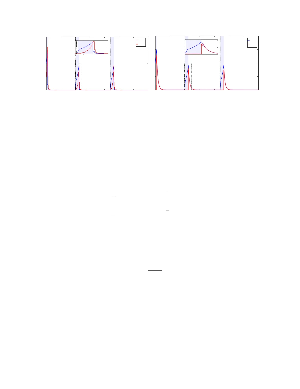
In put-to-state stabilization of linear sy stems under dat a-rate constraints Mahmoud Zamani and Guosong Y ang ∗ Abstract W e study f eedbac k stabilization of continuous-time linear sys tems under finite data-rate constraints in the presence of unkno wn disturbances. A communication and control strategy based on sampled and quantized state measurements is proposed, where the quantization range is dynamically adjusted using reachable-set propag ation and dis turbance estimates deriv ed from quantization parameters. The strategy alternates between stabilizing and searching stag es to handle escapes from the quantization rang e and emplo y s an additional quantization symbol to ensure robustness near the equilibr ium. It guarantees input-to-s tate s tability (ISS), impro ving upon e xisting results that yield onl y practical ISS or lack explicit data-rate conditions. Simulation results illustrate the effectiv eness of the strategy . 1 Introduction Feedbac k control under data-rate constraints has been an activ e research area f or decades, as sur v e yed in [ 1 – 3 ]. Such constraints arise naturally in netw ork ed control systems due to communication cos ts, bandwidth limitations, and security considerations. Be y ond these practical motivations, a fundamental question is ho w much inf ormation is required to achiev e a given control objectiv e. In this work, a finite data transmission rate is achie v ed b y g enerating the control input from sampled and quantized state measurements taking values in a finite set, which is a standard modeling framew ork. Earl y de v elopments f or linear sy stems include [ 4 – 10 ]. A central mechanism is dynamic quantization, in which the quantizer range is enlarged to recov er the state and then contracted to impro ve precision near the equilibr ium. This approach has been e xtended to nonlinear systems [ 11 – 13 ] and later to switched sys tems [ 14 – 16 ]. W e consider f eedbac k stabilization under data-rate constraints in the presence of unknown disturbances. In [ 7 , 10 ], disturbances are assumed to be bounded, and asymptotic stabilization is achie v ed with minimum data rates. The problem becomes significantl y more challenging without such bounds, as disturbances ma y drive the state outside the quantization range after capture. In this setting, [ 17 ] established input-to-state stability (ISS) [ 18 ] based on a dynamic quantization scheme with fixed center and alternating “zooming-out ” and “zooming-in” stag es. Similar ISS proper ties w ere achie v ed in [ 19 ] with impro v ed data-rate efficiency , using a mo ving-center quantizer with escape detection stag es and resets. More recentl y , [ 16 ] proposed an adaptiv e disturbance estimation scheme achie ving practical ISS f or switched linear sys tems. In this paper , w e propose a ne w approach to feedbac k stabilization under data-rate constraints with completel y unknown disturbances. Building on the disturbance estimation idea in [ 16 ], w e dev elop a ∗ The authors are with the Depar tment of Electrical and Computer Engineer ing, R utg ers Univ ersity , Piscata w a y , NJ 08854 US A (e-mails: {mahmoud.zamani, guosong.yang}@rutgers.edu ). 1 communication and control strategy that achie v es ISS f or linear sy stems. The ke y idea is to incor porate a disturbance estimate based on quantization parameters instead of constants, so that the state can escape the quantization rang e onl y when the disturbance is sufficiently larg e relativ e to both the quantization radius and the distance from its center to the equilibrium. The proposed s trategy uses an additional quantization symbol to handle states near the equilibr ium and ensure ISS. In contrast to e xisting approaches [ 17 , 19 ], our method pro vides an explicit bound on the admissible data rate and does not require quantizer resets or dedicated escape-detection stag es. The remainder of the paper is org anized as follo ws. Section 2 introduces the system model, inf ormation structure, and basic assumptions. Our main result is presented in Section 3 . Section 4 e xplains the communication and control strategy , with reachable-set approximations de v eloped in Section 5 . Section 6 pro vides the stability analy sis with major steps summarized as technical lemmas. A simulation e xample is giv en in Section 7 . N otations: The ∞ -nor m of a v ector v = ( v 1 , . . . , v n ) ∈ R n is denoted b y | v | := | v | ∞ = max 1 ≤ i ≤ n | v i | . The induced ∞ -norm of a matr ix M = [ a ij ] ∈ R n × n is denoted b y ∥ M ∥ := ∥ M ∥ ∞ = max 1 ≤ i ≤ n P n j =1 | a ij | . The larg es t and smallest eigen values of a symmetr ic matrix M ∈ R n × n are denoted b y λ ( M ) and λ ( M ) , respectiv el y . A continuous function γ : R ≥ 0 → R ≥ 0 is of class K ∞ , denoted b y γ ∈ K ∞ , if it is strictly increasing, unbounded, and satisfies γ (0) = 0 . The left limit of a piecewise continuous function z ( · ) at t is denoted b y z ( t − ) := lim s ↗ t z ( s ) . 2 Problem f ormulation 2.1 Sy stem definition Consider a continuous-time linear sys tem ˙ x = Ax + B u + D d, x (0) = x 0 , (1) where x ∈ R n x is the state, u ∈ R n u is the control input, and d ∈ R n d is an unkno wn disturbance. The disturbance d ( · ) is assumed to be Lebesgue measurable and locally essentially bounded. The essential supremum ∞ -nor m of d ( · ) o v er an interval J is denoted by ∥ d ∥ J := ess sup t ∈ J | d ( t ) | ; the subscr ipt is omitted when J = R ≥ 0 . Our first basic assumption is that the sys tem ( 1 ) is stabilizable. Assump tion 1 (Stabilizability) . The pair ( A, B ) is stabilizable, that is, there exis ts a state feedbac k gain matrix K such that A + B K is Hur witz (all eigen values ha v e negativ e real par ts). In what f ollo ws, we assume that such a matr ix K has been selected and fixed. 2.2 Inf ormation structure W e seek to generate a stabilizing control input u ( · ) based on limited inf ormation about the state x ( · ) . As sho wn in Fig. 1 , the feedbac k loop includes a sensor with an encoder and a controller with a decoder . The sensor samples the state at times t k = k τ s , k ∈ Z ≥ 0 , where τ s > 0 is a fixed sampling period . Each sample x ( t k ) is encoded as an integer i k ∈ { 0 , 1 , . . . , N n x + 1 } , where N > 0 is a fix ed integ er , and transmitted to 2 Figure 1: Information structure. the controller . The resulting data transmission rate is given by log 2 ( N n x + 2) τ s bits per unit time. This inf or mation str ucture enables a separation of sensing and control tasks, as the controller does not require access to the e xact state. Details of the communication and control strategy are pro vided in Section 4 . Our second basic assumption imposes a low er bound on the admissible data rate. Assump tion 2 (Data rate) . The sampling per iod τ s and the integer N satisfy Λ := ∥ e Aτ s ∥ < N . (2) The inequality in ( 2 ) can be view ed as a data-rate bound, as it requires the integer N to be sufficiently larg e relative to the sampling period τ s . Similar data-rate bounds ha v e appeared in [ 7 , 10 , 11 ] f or stabilizing linear sys tems and in [ 14 , 16 ] for stabilizing switched linear sys tems. The relationship among these bounds are discussed in [ 19 , Sec. V] and [ 14 , Sec. 2.2]. 3 Main result The control objective is to stabilize the sy stem defined in Section 2.1 under the inf ormation constraint described in Section 2.2 in a robust sense. Specificall y , we aim to achie v e input-to-stat e stability (ISS) , originally introduced in [ 18 ]. The theorem belo w adopts a characterization of ISS from [ 20 ]; see also [ 21 , Sec. 10.4] Theorem 1. Consider the linear syst em ( 1 ) . Suppose that Assumptions 1 and 2 hold. Then ther e exists a communication and control str at egy that render s the closed-loop syst em input-to-stat e stable, that is, the f ollowing holds: ther e exist functions γ 1 , γ 2 , γ 3 ∈ K ∞ suc h that for any initial condition x 0 ∈ R n x and any disturbance d ( · ) , the solution satisfies | x ( t ) | ≤ γ 1 ( | x 0 | ) + γ 2 ( ∥ d ∥ ) ∀ t ≥ 0 (3) and lim sup t →∞ | x ( t ) | ≤ γ 3  lim sup t →∞ | d ( t ) |  . (4) The communication and control strategy is presented in Section 4 . The K ∞ gain functions γ 1 , γ 2 , and γ 3 are giv en in ( 44 ) and ( 45 ) in the proof of Theorem 1 in Section 6.3 . 3 4 Communication and control strategy In this section, we descr ibe the communication and control strategy , assuming that suitable approximations of the reachable sets of the state are av ailable at all sampling times (these approximations are constructed in Section 5 ). The initial state x (0) = x 0 is unknown. At t 0 = 0 , both the sensor and the controller are initialized with x ∗ 0 = 0 and a design parameter E 0 > 0 . At each sampling time t k , the sensor chec ks whether | x ( t k ) − x ∗ k | ≤ E k , (5) that is, whether the state x ( t k ) lies in the hypercube R k := { v ∈ R n x : | v − x ∗ k | ≤ E k } . The set R k appro ximates the reachable set at t k and ser v es as the quantization range. If ( 5 ) holds, then the state is visible , and the system is in a stabilizing stag e (Section 4.1 ); other wise, the state is lost , and the sy stem is in a searc hing stag e (Section 4.2 ). If the state is visible at t k , then the sys tem remains in a stabilizing stag e until the first t j > t k such that x ( t j ) / ∈ R j , at which point the state escapes . Con v ersel y , if the state is lost at t k , then the sys tem remains in a searching stag e until the first t i > t k such that x ( t i ) ∈ R i , at which point the state is (r e)cap tur ed . Due to the unknown disturbance, the system ma y alter nate betw een stabilizing and searching stag es finitely or infinitel y man y times. 4.1 Stabilizing stages At each t k in a stabilizing stage, the sensor first chec ks whether | x ( t k ) | ≤ E k N . (6) If so, it transmits i k = 1 to the controller . Otherwise, it par titions R k into N n x equal h ypercubic cells (with N per dimension), assigns each cell a unique inde x from { 2 , . . . , N n x + 1 } , and transmits the inde x i k of the cell containing x ( t k ) . Each such cell has radius E k / N . U pon receiving i k ∈ { 1 , . . . , N n x + 1 } , the controller inf ers that ( 5 ) holds and reconstructs the cor re- sponding cell center c k using the same inde xing protocol. For i k ≥ 2 , we ha v e | x ( t k ) − c k | ≤ E k N (7) and | c k − x ∗ k | ≤ N − 1 N E k . (8) For i k = 1 , w e ha v e c k = 0 and ( 7 ) still holds. The controller then applies the control input u ( t ) = K ˆ x ( t ) , t ∈ [ t k , t k +1 ) , 4 where K is the stabilizing gain matr ix from Assumption 1 , and ˆ x ev olv es according to the auxiliar y system ˙ ˆ x = A ˆ x + B u, (9) with the boundar y condition ˆ x ( t k ) = c k . (10) Hence ˆ x is reset to c k at each t k in a stabilizing stage, and is in general only right-continuous. Finall y , both the sensor and the controller compute x ∗ k +1 := F ( c k ) , E k +1 := G ( E k , x ∗ k ) (11) without fur ther communication. The functions F and G , der iv ed in Section 5.1 , are designed to satisfy tw o proper ties. Firs t, the y ensure | x ( t k +1 ) − x ∗ k +1 | ≤ E k +1 (12) whene v er ∥ d ∥ [ t k ,t k +1 ] = 0 . Second, if the state escapes at t k +1 (i.e., ( 12 ) does not hold), the y provide bounds on | x ( t k +1 ) | and E k +1 in ter ms of ∥ d ∥ [ t k ,t k +1 ] . 4.2 Searc hing st ag es At each t k in a searching stage, the sensor transmits the “o v er flo w symbol” i k = 0 . Upon receiving i k = 0 , the controller inf ers that the state is lost and then applies the control input u ≡ 0 on [ t k , t k +1 ) . Finall y , both the sensor and the controller compute x ∗ k +1 := ˆ F ( x ∗ k ) , E k +1 := ˆ G ((1 + ε ) E k , δ ) (13) using design parameters ε, δ > 0 , without fur ther communication. The functions ˆ F and ˆ G , derived in Section 5.2 , are designed so that | x ( t k +1 ) − x ∗ k +1 | ≤ ˆ G ( | x ( t k ) − x ∗ k | , ∥ d ∥ [ t k ,t k +1 ] ) . (14) Hence the factor 1 + ε in ( 13 ) ensures that the growth rate of E k dominates that of | x ( t k ) − x ∗ k | . At an escape time t j , the computation of E j +1 is adjusted: the first argument of ˆ G is modified to enable comparison betw een δ and ∥ d ∥ [ t j − 1 ,t j +1 ] ; see Section 5.2 f or details. 5 Appro ximation of reachable sets In this section, w e der iv e recursiv e f ormulas f or propagating reachable-set appro ximations used in the communication and control strategy . 5 5.1 Stabilizing stages Consider a sampling time t k in a stabilizing stage, so that ( 5 ) holds. Define the er ror e := x − ˆ x . Combining ( 1 ) and ( 9 ) yields ˙ e = Ae + D d, | e ( t k ) | = | x ( t k ) − c k | ≤ E k N (15) on [ t k , t k +1 ) , where the boundar y condition f ollo ws from ( 7 ) and ( 10 ). Hence | e ( t − k +1 ) | =     e Aτ s e ( t k ) + Z t k +1 t k e A ( t k +1 − τ ) D d ( τ ) d τ     ≤ ∥ e Aτ s ∥| e ( t k ) | +  Z τ s 0 ∥ e As D ∥ d s  ∥ d ∥ [ t k ,t k +1 ] ≤ Λ N E k + Φ ∥ d ∥ [ t k ,t k +1 ] , (16) where Λ = ∥ e Aτ s ∥ as in ( 2 ) and Φ := Z τ s 0 ∥ e As D ∥ d s. (17) W e define the propagation functions as x ∗ k +1 = F ( c k ) := ˆ x ( t − k +1 ) = S c k , (18) where S := e ( A + B K ) τ s , and E k +1 = G ( E k , x ∗ k ) := Λ N E k + p ϕV k (19) with V k := V ( x ∗ k , E k ) := ( x ∗ k ) ⊤ P x ∗ k + ρE 2 k , (20) where ϕ, ρ > 0 are design parameters specified below . Because A + B K is Hur witz, there exis t positiv e definite symmetr ic matrices P , Q ∈ R n x × n x such that S ⊤ P S − P = − Q < 0 . (21) Define χ := 2 n 2 x ∥ S ⊤ P S ∥ 2 λ ( Q ) + n x ∥ S ⊤ P S ∥ . (22) W e select design parameters ψ , ρ, ϕ > 0 sequentiall y . As Λ < N in Assumption 2 , there e xists a sufficiently small ψ > 0 such that (1 + ψ ) Λ 2 N 2 < 1 , (23) and then a sufficiently larg e ρ > 0 suc h that ( N − 1) 2 N 2 χ ρ + (1 + ψ ) Λ 2 N 2 < 1 . (24) 6 Finall y , there exis ts a sufficiently small ϕ > 0 suc h that ν := max ( 1 − λ ( Q ) 2 λ ( P ) , ( N − 1) 2 N 2 χ ρ + (1 + ψ ) Λ 2 N 2 ) +  1 + 1 ψ  ϕρ (25) satisfies ν < 1 . 5.2 Searc hing st ag es Consider a sampling time t k in a searching stage. Combining ( 1 ) and ( 9 ) with u ≡ 0 and ˆ x ( t k ) = x ∗ k yields ˙ e = Ae + D d, | e ( t k ) | = | x ( t k ) − x ∗ k | (26) on [ t k , t k +1 ) . Hence | e ( t − k +1 ) | ≤ ∥ e Aτ s ∥| e ( t k ) | +  Z τ s 0 ∥ e As D ∥ d s  ∥ d ∥ [ t k ,t k +1 ] ≤ Λ | e ( t k ) | + Φ ∥ d ∥ [ t k ,t k +1 ] (27) where Λ and Φ are defined in ( 2 ) and ( 17 ), respectiv el y . W e define the propagation functions as x ∗ k +1 = ˆ F ( x ∗ k ) := ˆ x ( t − k +1 ) = ˆ S x ∗ k , (28) where ˆ S := e Aτ s , and, to dominate the g ro wth rate of | e ( t k ) | , E k +1 = ˆ G ((1 + ε ) E k , δ ) := (1 + ε )Λ E k + Φ δ, (29) where ε, δ > 0 are design parameters. At an escape time t j , the computation of E j +1 is adjusted to enable compar ison between δ and ∥ d ∥ [ t j − 1 ,t j +1 ] . Instead of using E j from ( 19 ) in the first argument, we let E j +1 = ˆ G ((1 + ε ) ˆ E j , δ ) (30) where ˆ E j := Λ N E j − 1 + Φ δ. In Section 6.2 , we sho w that the state is(re)captured in finite time under essentially bounded disturbances. The compar ison between δ and ∥ d ∥ [ t j − 1 ,t j +1 ] is established in the proof of Lemma 8 . 6 Stability analy sis In this section, w e establish Theorem 1 based on the communication and control strategy descr ibed in Section 4 . W e first present ke y steps of the proof as technical lemmas, f ollo wed by the proof of Theorem 1 in Section 6.3 . Throughout the anal y sis, w e assume that the essential supremum nor m ∥ d ∥ is finite, since other wise the bounds ( 3 ) and ( 4 ) hold tr ivially . W e also assume that Λ > 1 . 1 1 Since Λ = ∥ e Aτ s ∥ ≥ 1 , equality holds only if all eigen v alues of A hav e nonpositiv e real parts. The case Λ = 1 can be handled b y replacing Λ with max {∥ e Aτ s ∥ , 1 + ϵ Λ } for any ϵ Λ > 0 . 7 6.1 Stabilizing stages W e first establish e xponential decay of V k := V ( x ∗ k , E k ) defined in ( 20 ) dur ing stabilizing stages. Lemma 1. F or any sampling time t k in a stabilizing stag e, V k +1 ≤ ν V k , (31) wher e ν ∈ (0 , 1) is defined in ( 25 ) . Pr oof. See Appendix A.1 . W e next relate V k to | x ( t k ) | , | x ( t k +1 ) | , and E k . Lemma 2. There exist constants C 1 , C 2 , C 3 > 0 such that f or any sampling time t k in a stabilizing stag e, p V k ≤ C 1 ( | x ( t k ) | + E k ) , (32) | x ( t k ) | ≤ C 2 p V k , (33) | x ( t k +1 ) | ≤ C 3 p V k + Φ ∥ d ∥ [ t k ,t k +1 ] , (34) Pr oof. See Appendix A.2 . The next tw o lemmas provide an exponentiall y deca ying state bound and a state bound with suitable monotonicity and K ∞ proper ties. Lemma 3. Ther e exist constants C, λ > 0 such that f or any two sampling times t k > t l fr om the same stabilizing stag e, | x ( t k ) | ≤ C e − λ ( k − l ) ( | x ( t l ) | + E l ) + Φ ∥ d ∥ [ t k − 1 ,t k ] . (35) Pr oof. See Appendix A.3 . Lemma 4. There exist continuous functions χ x , χ d : R > 0 × R ≥ 0 → R ≥ 0 suc h that f or each fixed s > 0 , χ x ( · , s ) and χ d ( · , s ) are nondecr easing, for each fixed E > 0 , χ x ( E , · ) , χ d ( E , · ) ∈ K ∞ , and f or any two sampling times t k ≥ t l fr om the same stabilizing stag e, | x ( t k ) | ≤ χ x ( E l , | x ( t l ) | ) + χ d ( E l , ∥ d ∥ [ t l ,t k ] ) . (36) Pr oof. See Appendix A.4 . Finall y , we bound the state and quantization radius at escape times in ter ms of the disturbance ov er the preceding sampling inter v al, independently of the initial state. Lemma 5. There exists a constant Γ > 0 suc h that for any sampling time t j at whic h the state escapes, | x ( t j ) | ≤ Γ ∥ d ∥ [ t j − 1 ,t j ] , E j − 1 ≤ Γ ∥ d ∥ [ t j − 1 ,t j ] . (37) Pr oof. See Appendix A.5 . 8 6.2 Searc hing st ag es W e first sho w that if the state is lost at t 0 = 0 , then it is guaranteed to be captured in finite time. Lemma 6. If the state is lost at t 0 = 0 , then it is captur ed at some sampling time t i 0 satisfying i 0 ≤ max ( η x  | x 0 | E 0  , η d ∥ d ∥ [0 ,t i 0 ] δ !) , (38) wher e η x ( s ) := ( ⌈ log 1+ ε s ⌉ , s > 1 , 0 , 0 ≤ s ≤ 1 , η d ( s ) := ( ⌈ log 1+ ε ( r ε s ) ⌉ , s > 1 , 0 , 0 ≤ s ≤ 1 , with r ε := ˆ Λ − 1 Λ − 1 , ˆ Λ := (1 + ε )Λ . Pr oof. See Appendix A.6 . The ne xt lemma pro vides bounds on the state and the quantization radius at the first capture. Lemma 7. Ther e exist functions ˆ γ x 0 , ˆ γ d 0 ∈ K ∞ suc h that if the state is first captur ed at t i 0 , then f or any sampling time t k ≤ t i 0 , | x ( t k ) | ≤ ˆ γ x 0 ( | x 0 | ) + ˆ γ d 0 ( ∥ d ∥ [0 ,t i 0 ] ) . (39) Mor eo v er , there exists a continuous function ˆ χ E 0 : R > 0 × R ≥ 0 × R ≥ 0 → R > 0 suc h that f or eac h fixed E , s > 0 , ˆ χ E 0 ( E , s, · ) and ˆ χ E 0 ( E , · , s ) ar e nondecr easing, and E i 0 ≤ ˆ χ E 0 ( E 0 , | x 0 | , ∥ d ∥ [0 ,t i 0 ] ) . (40) Pr oof. See Appendix A.7 . W e now show that if the state escapes, then it is guaranteed to be recaptured in finite time. Lemma 8. If the state escapes at t j > 0 , then it is recap tur ed at some sampling time t i > t j satisfying i ≤ j + max ( η d ∥ d ∥ [ t j − 1 ,t i ] δ ! , 1 ) , (41) wher e η d is defined in Lemma 6 . Pr oof. See Appendix A.8 . The final lemma pro vides bounds on the state and the quantization radius at recapture. 9 Lemma 9. Ther e exist ˆ γ x , ˆ γ d ∈ K ∞ suc h that if the state escapes at t j and is recap tur ed at t i , then for any sampling time t k betw een t j and t i , | x ( t k ) | ≤ ˆ γ x ( | x ( t j ) | ) + ˆ γ d ( ∥ d ∥ [ t j − 1 ,t i ] ) . (42) Mor eo v er , ther e exists a continuous function ˆ χ E : R > 0 × R ≥ 0 → R > 0 suc h that for eac h fixed E > 0 , ˆ χ E ( E , · ) is nondecr easing, and E i ≤ ˆ χ E ( E j − 1 , ∥ d ∥ [ t j − 1 ,t i ] ) . (43) Pr oof. See Appendix A.9 . 6.3 Proof of Theorem 1 W e inde x the alter nating searching and stabilizing stag es as follo ws. Let 0 ≤ i 0 < j 1 < i 1 < · · · be such that the state is first captured at t i 0 , escapes at t j l , and is recaptured at t i l f or l ≥ 1 . By Lemma 6 , we hav e i 0 < ∞ . If the state nev er escapes after some t i l , w e set j l +1 = ∞ . By Lemma 8 , if j l < ∞ then i l < ∞ . Firs t, we establish the bound ( 3 ) at sampling times b y constructing the functions γ 1 , γ 2 ∈ K ∞ . First searching st ag e [0 , t i 0 ) Assume without loss of generality that the state is lost at t 0 = 0 ; otherwise, set i 0 = 0 . By Lemma 7 , for all t k ≤ t i 0 , the bound ( 39 ) holds. First stabilizing st ag e [ t i 0 , t j 1 ) At t i 0 , Lemma 7 yields | x ( t i 0 ) | ≤ ˆ γ x 0 ( | x 0 | ) + ˆ γ d 0 ( ∥ d ∥ [0 ,t i 0 ] ) , and E i 0 ≤ ˆ χ E 0 ( E 0 , | x 0 | , ∥ d ∥ [0 ,t i 0 ] ) . From Lemma 4 , f or any t i 0 ≤ t k < t j 1 , | x ( t k ) | ≤ χ x ( E i 0 , | x ( t i 0 ) | ) + χ d ( E i 0 , ∥ d ∥ [ t i 0 ,t k ] ) ≤ χ x  ˆ χ E 0 ( E 0 , | x 0 | , ∥ d ∥ [0 ,t i 0 ] ) , ˆ γ x 0 ( | x 0 | ) + ˆ γ d 0 ( ∥ d ∥ [0 ,t i 0 ] )  + χ d  ˆ χ E 0 ( E 0 , | x 0 | , ∥ d ∥ [0 ,t i 0 ] ) , ∥ d ∥ [ t i 0 ,t k ]  . Using the abo v e bounds, a standard compar ison-function argument yields continuous functions ¯ χ 1 , ¯ χ 2 : R > 0 × R ≥ 0 → R ≥ 0 such that f or each fixed E > 0 , ¯ χ 1 ( E , · ) , ¯ χ 2 ( E , · ) ∈ K ∞ , and ¯ χ 1 ( E 0 , | x 0 | ) + ¯ χ 2 ( E 0 , ∥ d ∥ [0 ,t k ] ) ≥ χ x  ˆ χ E 0 ( E 0 , | x 0 | , ∥ d ∥ [0 ,t k ] ) , ˆ γ x 0 ( | x 0 | ) + ˆ γ d 0 ( ∥ d ∥ [0 ,t k ] )  + χ d  ˆ χ E 0 ( E 0 , | x 0 | , ∥ d ∥ [0 ,t k ] ) , ∥ d ∥ [0 ,t k ]  , which implies | x ( t k ) | ≤ ¯ χ 1 ( E 0 , | x 0 | ) + ¯ χ 2 ( E 0 , ∥ d ∥ [0 ,t k ] ) . If t j 1 = ∞ , then the proof of ( 3 ) is complete. Other wise, consider an arbitrary escape time t j l < ∞ . 10 Searc hing st age [ t j l , t i l ) At t j l , Lemma 5 yields | x ( t j l ) | ≤ Γ ∥ d ∥ [ t j l − 1 ,t j l ] , E j l − 1 ≤ Γ ∥ d ∥ [ t j l − 1 ,t j l ] . From Lemma 9 , f or any t j l ≤ t k ≤ t i l , | x ( t k ) | ≤ ˆ γ x ( | x ( t j l ) | ) + ˆ γ d ( ∥ d ∥ [ t j l − 1 ,t i l ] ) ≤ ˆ γ x (Γ ∥ d ∥ [ t j l − 1 ,t j l ] ) + ˆ γ d ( ∥ d ∥ [ t j l − 1 ,t i l ] ) ≤ ˆ γ ( ∥ d ∥ [ t j l − 1 ,t i l ] ) , where ˆ γ ( s ) := ˆ γ x (Γ s ) + ˆ γ d ( s ) ∈ K ∞ . Stabilizing st ag e [ t i l , t j l +1 ) At t i l , | x ( t i l ) | ≤ ˆ γ ( ∥ d ∥ [ t j l − 1 ,t i l ] ) , and Lemma 9 yields E i l ≤ ˆ χ E ( E j l − 1 , ∥ d ∥ [ t j l − 1 ,t i l ] ) ≤ ˆ χ E (Γ ∥ d ∥ [ t j l − 1 ,t j l ] , ∥ d ∥ [ t j l − 1 ,t i l ] ) . From Lemma 4 , f or any t i l ≤ t k < t j l +1 , | x ( t k ) | ≤ χ x ( E i l , | x ( t i l ) | ) + χ d ( E i l , ∥ d ∥ [ t i l ,t k ] ) ≤ χ x  ˆ χ E (Γ ∥ d ∥ [ t j l − 1 ,t j l ] , ∥ d ∥ [ t j l − 1 ,t i l ] ) , ˆ γ ( ∥ d ∥ [ t j l − 1 ,t i l ] )  + χ d  ˆ χ E (Γ ∥ d ∥ [ t j l − 1 ,t j l ] , ∥ d ∥ [ t j l − 1 ,t i l ] ) , ∥ d ∥ [ t i l ,t k ]  ≤ ¯ γ ( ∥ d ∥ [ t j l − 1 ,t k ] ) , where ¯ γ ( s ) := χ x ( ˆ χ E (Γ s, s ) , ˆ γ ( s )) + χ d ( ˆ χ E (Γ s, s ) , s ) ∈ K ∞ . By induction ov er consecutive searching and stabilizing stages, the bound ( 3 ) holds f or all sampling times with the K ∞ functions γ 1 ( s ) := max { ˆ γ x 0 ( s ) , ¯ χ 1 ( E 0 , s ) } , γ 2 ( s ) := max { ˆ γ d 0 ( s ) , ¯ χ 2 ( E 0 , s ) , ˆ γ ( s ) , ¯ γ ( s ) } . (44) Ne xt, w e establish the bound ( 4 ) at sampling times b y constructing the function γ 3 ∈ K ∞ . If only finitel y man y searching stag es occur , then after some time the sys tem remains in a stabilizing stag e, and Lemma 3 implies lim sup k →∞ | x ( t k ) | ≤ Φ lim sup t →∞ | d ( t ) | . If infinitely man y searching stag es occur , then the bounds abo v e imply that, after each escape time t j l , | x ( t k ) | ≤ ˆ γ ( ∥ d ∥ [ t j l − 1 ,t i l ] ) ∀ j l ≤ k ≤ i l , | x ( t k ) | ≤ ¯ γ ( ∥ d ∥ [ t j l − 1 ,t k ] ) ∀ i l ≤ k < j l +1 . 11 Theref ore, lim sup k →∞ | x ( t k ) | ≤ γ 3  lim sup t →∞ | d ( t ) |  with the K ∞ function γ 3 ( s ) := max { Φ s, ˆ γ ( s ) , ¯ γ ( s ) } . (45) The e xtension of ( 3 ) and ( 4 ) to all t ≥ 0 f ollo ws from standard arguments. Specifically , for any t ≥ 0 , let k be such that t ∈ [ t k , t k +1 ) . W e first consider the case that the sys tem is in a stabilizing stage at t k and c k  = 0 . From ( 9 ) and ( 15 ), | x ( t ) | ≤ | ˆ x ( t ) | + | e ( t ) | ≤ ∥ e ( A + B K )( t − t k ) ∥| c k | + ∥ e A ( t − t k ) ∥| e ( t k ) | +  Z t 0 ∥ e As D ∥ d s  ∥ d ∥ [ t k ,t ] ≤ ¯ Λ | c k | + ˜ Λ N E k + Φ ∥ d ∥ [ t k ,t ] , where ¯ Λ := max 0 ≤ s ≤ τ s ∥ e ( A + B K ) s ∥ , ˜ Λ := max 0 ≤ s ≤ τ s ∥ e As ∥ . By ( 7 ), | c k | ≤ | x ( t k ) | + | x ( t k ) − c k | ≤ | x ( t k ) | + E k N , and since ( 6 ) fails at t k , | x ( t k ) | > E k N . Hence | x ( t ) | ≤ ˜ H | x ( t k ) | + Φ ∥ d ∥ [ t k ,t ] . (46) with ˜ H := 2 ¯ Λ + ˜ Λ . If the sys tem is in a stabilizing stag e at t k and c k = 0 , or the system is in a searching stag e at t k , then u ≡ 0 on [ t k , t k +1 ) , and | x ( t ) | ≤ ∥ e A ( t − t k ) ∥| x ( t k ) | +  Z τ s 0 ∥ e As D ∥ d s  ∥ d ∥ [ t k ,t ] ≤ ˜ Λ | x ( t k ) | + Φ ∥ d ∥ [ t k ,t ] , so ( 46 ) still holds. Since the bound ( 3 ) holds for all sampling times with the K ∞ functions γ 1 and γ 2 defined in ( 44 ), by ( 46 ), it holds f or all t ≥ 0 with the K ∞ functions γ 1 ( s ) := ˜ H max { ˆ γ x 0 ( s ) , ¯ χ 1 ( E 0 , s ) } , γ 2 ( s ) := ˜ H max { ˆ γ d 0 ( s ) , ¯ χ 2 ( E 0 , s ) , ˆ γ ( s ) , ¯ γ ( s ) } + Φ s. 12 Since lim sup k →∞ | x ( t k ) | ≤ γ 3  lim sup t →∞ | d ( t ) |  with the K ∞ functions γ 3 defined in ( 45 ), by ( 46 ), lim sup t →∞ | x ( t ) | ≤ lim sup k →∞ ˜ H | x ( t k ) | + Φ ∥ d ∥ [ t k ,t k +1 ] ≤ lim sup k →∞ ˜ H | x ( t k ) | + Φ lim sup t →∞ | d ( t ) | , which implies the bound ( 4 ) with the K ∞ function γ 3 ( s ) := ˜ H max { Φ s, ˆ γ ( s ) , ¯ γ ( s ) } + Φ s. 7 Simulation exam ple W e illustrate the proposed communication and control strategy on the linear sy stem ( 1 ) with A = " 1 0 0 − 1 . 5 # , B = " 1 0 . 5 # , D = " 1 0 # , K = h − 3 . 5 0 i , sampling per iod τ s = 0 . 1 s, and integer N = 5 , which satisfy Assumptions 1 and 2 . The design parameters are chosen to satisfy the conditions in Section 5 : E 0 = 0 . 5 , ε = 0 . 2 , δ = 0 . 1 , ψ = 0 . 2 , ρ = 0 . 1 , ϕ = 0 . 01 . W e simulate the sy stem with initial state x 0 = " 1 1 # , so the state is initially lost. T o induce escape and reco v er y ev ents, disturbance pulses with d ( t ) = 1 . 5 are applied on [10 . 5 , 10 . 7] s and [22 . 5 , 22 . 7] s, and d ( t ) = 0 otherwise. Figure 2 ( a ) sho w s the er ror | e ( t ) | = | x ( t ) − ˆ x ( t ) | (blue) and quantization radius E k (red). During stabilizing stag es, both | e ( t k ) | and E k at sampling times deca y exponentiall y; | e ( t ) | ma y increase betw een sampling times; E k are only computed at sampling times and plotted as step functions. Disturbance pulses (onsets indicated by black dashed lines) cause shar p increases in | e ( t ) | , leading to | e ( t k ) | > E k and loss of the state. During searching stages (shaded regions), the gro wth of E k dominates that of | e ( t k ) | , enabling recapture of the state. Figure 2 ( b ) sho ws the state x 1 ( t ) (blue) and auxiliar y state ˆ x 1 ( t ) (red). During stabilizing stag es, x 1 ( t ) is dr iv en to w ards zero (it could exhibit temporary increase due to the quantization er ror); ˆ x 1 ( t ) decreases continuously between sampling times but e xhibits discontinuities at sampling times due to ne w measurements. Dur ing searching stages (shaded regions), x 1 ( t ) and ˆ x 1 ( t ) both grow (the latter is unclear since the v alues are small). These behaviors are consistent with the ISS proper ties established in Theorem 1 . 13 0 5 10 15 20 25 30 35 0 0.5 1 1.5 2 j e ( t ) j E k 10 10.5 11 1 1.5 12 0 0.5 1 (a) 0 5 10 15 20 25 30 0 0.5 1 1.5 x 1 ( t ) ^ x 1 ( t ) 10 10.5 11 1 1.5 12 0 0.5 1 (b) Figure 2: ( a ) Er ror | e ( t ) | = | x ( t ) − ˆ x ( t ) | (blue) and quantization radius E k (red). ( b ) State x 1 ( t ) (blue) and auxiliar y state ˆ x 1 ( t ) (red). Blac k dashed lines indicate disturbances onsets. Shaded regions indicate searching stag es. The zoomed-in plots highlight the searching stage and subsequent recapture after the first escape. A Proofs of technical lemmas W e first recall sev eral basic f acts from linear algebra used throughout the proofs. For any v , w ∈ R n , the ∞ -norm satisfies | v | 2 ≤ v ⊤ v , v ⊤ w ≤ n | v || w | . (47) For any symmetr ic matr ix M ∈ R n × n and an y v ∈ R n , λ ( M ) v ⊤ v ≤ v ⊤ M v ≤ λ ( M ) v ⊤ v , (48) which yields λ ( M ) | v | 2 ≤ v ⊤ M v ≤ n λ ( M ) | v | 2 . (49) A.1 Proof of Lemma 1 W e first consider the case c k  = 0 . From the propagation function ( 18 ), x ∗ k +1 = S c k = S ( x ∗ k + ∆ k ) , ∆ k := c k − x ∗ k , where | ∆ k | ≤ N − 1 N E k b y ( 8 ). Then ( x ∗ k +1 ) ⊤ P x ∗ k +1 = ( x ∗ k + ∆ k ) ⊤ S ⊤ P S ( x ∗ k + ∆ k ) = ( x ∗ k ) ⊤ S ⊤ P S x ∗ k + 2( x ∗ k ) ⊤ S ⊤ P S ∆ k + ∆ ⊤ k S ⊤ P S ∆ k . 14 Using the L yapuno v equation ( 21 ) and bounds ( 48 ) and ( 49 ), w e obtain ( x ∗ k ) ⊤ S ⊤ P S x ∗ k = ( x ∗ k ) ⊤ ( P − Q ) x ∗ k = ( x ∗ k ) ⊤ P x ∗ k − 1 2 ( x ∗ k ) ⊤ Qx ∗ k − 1 2 ( x ∗ k ) ⊤ Qx ∗ k ≤ 1 − λ ( Q ) 2 λ ( P ) ! ( x ∗ k ) ⊤ P x ∗ k − 1 2 λ ( Q ) | x ∗ k | 2 . Moreo v er, b y ( 47 ), 2( x ∗ k ) ⊤ S ⊤ P S ∆ k ≤ 2 n x | x ∗ k |∥ S ⊤ P S ∥| ∆ k | , ∆ ⊤ k S ⊤ P S ∆ k ≤ n x ∥ S ⊤ P S ∥| ∆ k | 2 . Combining the bounds and completing the square yields ( x ∗ k +1 ) ⊤ P x ∗ k +1 ≤  1 − λ ( Q ) 2 λ ( P )  ( x ∗ k ) ⊤ P x ∗ k − 1 2 λ ( Q ) | x ∗ k | 2 + 2 n x | x ∗ k |∥ S ⊤ P S ∥| ∆ k | + n x ∥ S ⊤ P S ∥| ∆ k | 2 ≤  1 − λ ( Q ) 2 λ ( P )  ( x ∗ k ) ⊤ P x ∗ k + χ | ∆ k | 2 −  r 1 2 λ ( Q ) | x ∗ k | − √ 2 n x ∥ S ⊤ P S ∥ p λ ( Q ) | ∆ k |  2 ≤  1 − λ ( Q ) 2 λ ( P )  ( x ∗ k ) ⊤ P x ∗ k + ( N − 1) 2 N 2 χE 2 k , where χ is defined in ( 22 ). Ne xt, from the propag ation function ( 19 ) and Y oung’ s inequality , E 2 k +1 =  Λ N E k + p ϕV k  2 ≤ (1 + ψ ) Λ 2 N 2 E 2 k +  1 + 1 ψ  ϕV k where ψ > 0 is chosen according to ( 23 ). Finall y , combining both bounds in V k +1 = ( x ∗ k +1 ) ⊤ P x ∗ k +1 + ρE 2 k +1 yields V k +1 ≤ ν V k , where ν is defined in ( 25 ). If c k = 0 , then x ∗ k +1 = S c k = 0 , and V k +1 = ρE 2 k +1 ≤ (1 + ψ ) Λ 2 N 2 +  1 + 1 ψ  ϕρ ! V k , so ( 31 ) still holds. 15 A.2 Proof of Lemma 2 W e first pro v e ( 32 ). Since V k = ( x ∗ k ) ⊤ P x ∗ k + ρE 2 k , the upper bound in ( 49 ) yields p V k ≤ q n x λ ( P ) | x ∗ k | + √ ρE k , where w e used √ a + b ≤ √ a + √ b . Moreo v er , by ( 5 ), | x ∗ k | ≤ | x ( t k ) | + | x ( t k ) − x ∗ k | ≤ | x ( t k ) | + E k . Hence ( 32 ) holds with C 1 := q n x λ ( P ) + √ ρ. Ne xt, we establish ( 33 ). From ( 5 ), | x ( t k ) | ≤ | x ∗ k | + | x ( t k ) − x ∗ k | ≤ | x ∗ k | + E k . Using the lo w er bound in ( 49 ), w e obtain | x ∗ k | ≤ s V k λ ( P ) , E k ≤ s V k ρ which yields ( 33 ) with C 2 := 1 p λ ( P ) + 1 √ ρ . Finall y , we pro v e ( 34 ). From the er ror estimate ( 16 ) and propagation function ( 18 ), | x ( t k +1 ) | ≤ | ˆ x ( t − k +1 ) | + | e ( t − k +1 ) | ≤ ∥ S ∥| c k | + Λ N E k + Φ ∥ d ∥ [ t k ,t k +1 ] . W e first consider the case c k  = 0 . By ( 8 ) and the lo w er bound in ( 49 ), | c k | ≤ | x ∗ k | + | c k − x ∗ k | ≤ | x ∗ k | + N − 1 N E k . Bounding | x ∗ k | and E k in ter ms of V k yields ( 34 ) with C 3 := max ( ∥ S ∥ p λ ( P ) , ( N − 1) ∥ S ∥ + Λ N √ ρ ) . If c k = 0 , then ˆ x ( t − k +1 ) = S c k = 0 , and | x ( t k +1 ) | = | e ( t − k +1 ) | ≤ Λ N E k + Φ ∥ d ∥ [ t k ,t k +1 ] , so ( 34 ) still holds. 16 A.3 Proof of Lemma 3 By iterating Lemma 1 , we obtain V k − 1 ≤ ν k − 1 − l V l , where ν ∈ (0 , 1) . Appl ying ( 32 ) at t l and ( 34 ) at t k − 1 yields | x ( t k ) | ≤ C 3 q V k − 1 + Φ ∥ d ∥ [ t k − 1 ,t k ] ≤ C 3 ν ( k − l − 1) / 2 p V l + Φ ∥ d ∥ [ t k − 1 ,t k ] ≤ C 1 C 3 ν ( k − l − 1) / 2 ( | x ( t l ) | + E l ) + Φ ∥ d ∥ [ t k − 1 ,t k ] . Hence ( 35 ) holds with C := C 1 C 3 ν − 1 / 2 , λ := − 1 2 ln ν > 0 . A.4 Proof of Lemma 4 W e consider tw o cases depending on whether the initial state dominates the disturbance. Case 1: | x ( t l ) | > Φ ∥ d ∥ [ t l ,t k ] . Let H := 2 ∥ S ∥ + Λ > 1 . Then log ν H < 0 since ν ∈ (0 , 1) . Fix any κ ∈ (0 , − 1 / log ν H ) , and define l x := max {⌈ κ log ν | x ( t l ) |⌉ , 0 } . Then ν l x ≤ | x ( t l ) | κ f or all | x ( t l ) | > 0 . W e distinguish between the “long-time ” regime k ≥ l + l x and the “shor t-time ” regime k < l + l x . If k ≥ l + l x , iterating Lemma 1 yields V k ≤ ν k − l V l ≤ ν l x V l ≤ | x ( t l ) | κ V l . Appl ying ( 32 ) at t l and ( 33 ) at t k , w e obtain | x ( t k ) | ≤ C 2 p V k ≤ C 2 | x ( t l ) | κ/ 2 p V l ≤ C 1 C 2 | x ( t l ) | κ/ 2 ( | x ( t l ) | + E l ) =: χ x 1 ( E l , | x ( t l ) | ) , where χ x 1 ( · , s ) is nondecreasing for each fixed s > 0 and χ x 1 ( E , · ) ∈ K ∞ f or each fix ed E > 0 . If l ≤ k < l + l x , we first consider the case c k  = 0 . From the er ror estimate ( 16 ) and propagation function ( 18 ), | x ( t k +1 ) | ≤ | ˆ x ( t − k +1 ) | + | e ( t − k +1 ) | ≤ ∥ S ∥| c k | + Λ N E k + Φ ∥ d ∥ [ t k ,t k +1 ] . By ( 7 ), | c k | ≤ | x ( t k ) | + | x ( t k ) − c k | ≤ | x ( t k ) | + E k N , 17 and since ( 6 ) fails at t k , | x ( t k ) | > E k N . Hence | x ( t k +1 ) | ≤ H | x ( t k ) | + Φ ∥ d ∥ [ t k ,t k +1 ] . (50) If c k = 0 , then u ≡ 0 on [ t k , t k +1 ) , and | x ( t k +1 ) | ≤ ∥ e Aτ s ∥| x ( t k ) | +  Z τ s 0 ∥ e As D ∥ d s  ∥ d ∥ [ t k ,t k +1 ] ≤ Λ | x ( t k ) | + Φ ∥ d ∥ [ t k ,t k +1 ] , so ( 50 ) still holds. Since ( 50 ) holds f or all sampling times between t l and t k , iterating it yields | x ( t k ) | ≤ H k − l | x ( t l ) | + H k − l − 1 H − 1 Φ ∥ d ∥ [ t l ,t k ] ≤ H k − l +1 − 1 H − 1 | x ( t l ) | ≤ H l x − 1 H − 1 | x ( t l ) | =: χ x 2 ( | x ( t l ) | ) . If | x ( t l ) | = s < 1 , then l x < κ log ν s + 1 , and χ x 2 ( s ) < H κ log ν s +1 H − 1 s = H H − 1 s κ log ν H +1 =: χ x 3 ( s ) . where χ x 3 ∈ K ∞ since κ log ν H + 1 > 0 . If | x ( t l ) | = s ≥ 1 , then l x = 0 , and χ x 2 ( s ) = 0 < χ x 3 ( s ) . Finall y , | x ( t k ) | ≤ max { χ x 1 ( E l , | x ( t l ) | ) , χ x 3 ( | x ( t l ) | ) } =: χ x ( E l , | x ( t l ) | ) , which satisfies the stated monotonicity and K ∞ proper ties. Case 2: | x ( t l ) | ≤ Φ ∥ d ∥ [ t l ,t k ] . The proof f ollo w s the same steps as in Case 1 and is omitted f or brevity . It yields analogous functions χ d 1 and χ d 3 such that | x ( t k ) | ≤ max { χ d 1 ( E l , ∥ d ∥ [ t l ,t k ] ) , χ d 3 ( ∥ d ∥ [ t l ,t k ] | ) } =: χ d ( E l , ∥ d ∥ [ t l ,t k ] ) , which satisfies the stated monotonicity and K ∞ proper ties. Combining the tw o cases yields ( 36 ). 18 A.5 Proof of Lemma 5 Since ( 5 ) holds at t j − 1 but fails at t j , | e ( t j ) | = | x ( t j ) − x ∗ j | > E j . Appl ying the er ror estimate ( 16 ) and propagation function ( 19 ) at t j − 1 , w e obtain Λ N E j − 1 + Φ ∥ d ∥ [ t j − 1 ,t j ] > Λ N E j − 1 + q ϕV j − 1 , that is, q ϕV j − 1 < Φ ∥ d ∥ [ t j − 1 ,t j ] . Theref ore, E j − 1 ≤ s V j − 1 ρ < 1 √ ρϕ Φ ∥ d ∥ [ t j − 1 ,t j ] . Ne xt, applying ( 34 ) at t j − 1 yields | x ( t j ) | ≤ C 3 q V j − 1 + Φ ∥ d ∥ [ t j − 1 ,t j ] <  C 3 √ ϕ + 1  Φ ∥ d ∥ [ t j − 1 ,t j ] . Combining the tw o bounds, w e obtain ( 37 ) with Γ := max  1 √ ρϕ , C 3 √ ϕ + 1  Φ > 0 , where C 3 > 0 is from Lemma 2 . A.6 Proof of Lemma 6 Let t k > 0 be a sampling time such that the state has not yet been captured by t k . Then the sys tem remains in a searching stag e on [0 , t k ) , and iterating the er ror estimate ( 27 ) and propagation functions ( 28 ) and ( 29 ) from 0 to t k with x ∗ 0 = 0 yields | e ( t − k ) | ≤ Λ k | x 0 | + Λ k − 1 Λ − 1 Φ ∥ d ∥ [0 ,t k ] , E k = ˆ Λ k E 0 + ˆ Λ k − 1 ˆ Λ − 1 Φ δ. Let i ∗ 0 be the smallest positive integer such that i ∗ 0 ≥ max    η x  | x 0 | E 0  , η d   ∥ d ∥ [0 ,t i ∗ 0 ] δ      . Such an integer exis ts if ∥ d ∥ is finite. W e sho w that the state is captured no later than t i ∗ 0 . 19 Firs t, since i ∗ 0 ≥ η x ( | x 0 | /E 0 ) , ˆ Λ i ∗ 0 E 0 = Λ i ∗ 0 (1 + ε ) i ∗ 0 E 0 ≥ Λ i ∗ 0 (1 + ε ) η x ( | x 0 | /E 0 ) E 0 ≥ Λ i ∗ 0 | x 0 | . Second, if δ < ∥ d ∥ [0 ,t i ∗ 0 ] , then i ∗ 0 ≥ η d   ∥ d ∥ [0 ,t i ∗ 0 ] δ   ≥ log 1+ ε   r ε ∥ d ∥ [0 ,t i ∗ 0 ] δ   , and ˆ Λ i ∗ 0 − 1 ˆ Λ − 1 δ > Λ i ∗ 0 − 1 ˆ Λ − 1 (1 + ε ) i ∗ 0 δ = Λ i ∗ 0 − 1 Λ − 1 (1 + ε ) i ∗ 0 r ε δ ≥ Λ i ∗ 0 − 1 Λ − 1 ∥ d ∥ [0 ,t i ∗ 0 ] . Otherwise, δ ≥ ∥ d ∥ [0 ,t i ∗ 0 ] , and since ˆ Λ > Λ , ˆ Λ i ∗ 0 − 1 ˆ Λ − 1 δ ≥ Λ i ∗ 0 − 1 Λ − 1 ∥ d ∥ [0 ,t i ∗ 0 ] . Combining these bounds yields E i ∗ 0 ≥ | e ( t i ∗ 0 ) | . Hence the state is captured at some sampling time t i 0 ≤ t i ∗ 0 . If i 0 < i ∗ 0 , then ( 38 ) f ollo w s immediately . If i 0 = i ∗ 0 , then i 0 − 1 < max ( η x  | x 0 | E 0  , η d ∥ d ∥ [0 ,t i 0 − 1 ] δ !) , and since both sides are integers, ( 38 ) still holds. A.7 Proof of Lemma 7 Since Consider an y t k ≤ t i 0 . the state is first captured at t i 0 , the sys tem remains in a searching stag e on [0 , t i 0 ) . Firs t, iterating the er ror estimate ( 27 ) and propagation function ( 28 ) from 0 to t k with x ∗ 0 = 0 yields | x ( t k ) | ≤ Λ k | x 0 | + Λ k − 1 Λ − 1 Φ ∥ d ∥ [0 ,t k ] ≤ Λ i 0 | x 0 | + Λ i 0 − 1 Λ − 1 Φ ∥ d ∥ [0 ,t i 0 ] . Substituting the bound on i 0 from ( 38 ) into the r ight-hand side, w e obtain a bound on | x ( t k ) | that is nondecreasing in | x 0 | and ∥ d ∥ [0 ,t i 0 ] and v anishes when | x 0 | = ∥ d ∥ [0 ,t i 0 ] = 0 . Theref ore, it can be dominated b y K ∞ functions ˆ γ x 0 ( | x 0 | ) + ˆ γ d 0 ( ∥ d ∥ [0 ,t i 0 ] ) using a standard compar ison-function construction, which pro v es ( 39 ). 20 Second, iterating the propagation function ( 29 ) from 0 to t i 0 yields E i 0 = ˆ Λ i 0 E 0 + ˆ Λ i 0 − 1 ˆ Λ − 1 Φ δ. Substituting again the bound on i 0 from ( 38 ) into the r ight-hand side, we obtain a bound on E i 0 that, f or each fix ed E 0 > 0 , is nondecreasing in | x 0 | and ∥ d ∥ [0 ,t i 0 ] . Theref ore, b y another standard compar ison-function construction, there e xists a continuous function ˆ χ E 0 : R > 0 × R ≥ 0 × R ≥ 0 → R > 0 with the stated monotonicity proper ty such that ( 40 ) holds. A.8 Proof of Lemma 8 If the state is recaptured at t j +1 , then i = j + 1 and ( 41 ) holds. In the remainder of the proof, we assume that the state is not recaptured at t j +1 . The sys tem remains in a searching stag e on [ t j , t i ) . Applying the same argument as in the proof of Lemma 6 , with the adjustment at t j according to ( 30 ), we obtain i ≤ j + max ( η x | e ( t j ) | ˆ E j ! , η d ∥ d ∥ [ t j ,t i ] δ ! , 1 ) , (51) where η x , η d are defined in Lemma 6 and satisfy η x ( s ) ≤ η d ( s ) f or all s ≥ 0 . Ne xt, applying the searching-stag e er ror estimate ( 27 ) at t j and the stabilizing-stag e er ror estimate ( 16 ) at t j − 1 yields | e ( t j +1 ) | ≤ Λ | e ( t j ) | + Φ ∥ d ∥ [ t j ,t j +1 ] ≤ Λ 2 N | e ( t j − 1 ) | + (Λ + 1)Φ ∥ d ∥ [ t j − 1 ,t j +1 ] . Moreo v er, from the adjusted propagation function ( 30 ), E j +1 = ˆ Λ ˆ E j + Φ δ = ˆ ΛΛ N E j − 1 + ( ˆ Λ + 1)Φ δ, where ˆ Λ = (1 + ε )Λ . Since the state escapes at t j and is not recaptured at t j +1 , | e ( t j − 1 ) | ≤ E j − 1 , | e ( t j +1 ) | > E j +1 , and the abo v e bounds imply δ < ∥ d ∥ [ t j − 1 ,t j +1 ] . Consequentl y , | e ( t j ) | ˆ E j ≤ Λ N | e ( t j − 1 ) | + Φ ∥ d ∥ [ t j − 1 ,t j +1 ] Λ N E j − 1 + Φ δ < ∥ d ∥ [ t j − 1 ,t j +1 ] δ , and thus η x | e ( t j ) | ˆ E j ! ≤ η x ∥ d ∥ [ t j − 1 ,t j +1 ] δ ! ≤ η d ∥ d ∥ [ t j − 1 ,t j +1 ] δ ! . Substituting this bound into ( 51 ) yields ( 41 ). 21 A.9 Proof of Lemma 9 Since the state escapes at t j and is recaptured at t i , the system remains in a searching stage on [ t j , t i ) . Consider an y sampling time t k ∈ [ t j , t i ) . Firs t, since u ≡ 0 on [ t j , t i ) , the state satisfies ˙ x = Ax + D d, and thus | x ( t k +1 ) | ≤ Λ | x ( t k ) | + Φ ∥ d ∥ [ t k ,t k +1 ] . Iterating this bound from t j to t k yields | x ( t k ) | ≤ Λ k − j | x ( t j ) | + Λ k − j − 1 Λ − 1 Φ ∥ d ∥ [ t j ,t k ] ≤ Λ i − j | x ( t j ) | + Λ i − j − 1 Λ − 1 Φ ∥ d ∥ [ t j ,t i ] . Substituting the bound on i from ( 41 ): i ≤ j + max ( η d ∥ d ∥ [ t j − 1 ,t i ] δ ! , 1 ) , into the r ight-hand side, w e obtain a bound on | x ( t k ) | that is nondecreasing in | x ( t j ) | and ∥ d ∥ [ t j − 1 ,t i ] and v anishes when | x ( t j ) | = ∥ d ∥ [ t j − 1 ,t i ] = 0 . Theref ore, it can be dominated by K ∞ functions ˆ γ x ( | x ( t j ) | ) + ˆ γ d ( ∥ d ∥ [ t j − 1 ,t i ] ) using a standard comparison-function constr uction, which pro v es ( 42 ). Second, iterating the propagation function ( 29 ) from t j to t i , with the adjustment at t j according to ( 30 ), yields E i = ˆ Λ i − j ˆ E j + ˆ Λ i − j − 1 ˆ Λ − 1 Φ δ = ˆ Λ i − j Λ N E j − 1 + ˆ Λ i − j +1 − 1 ˆ Λ − 1 Φ δ. Substituting again the bound on i from ( 41 ), w e obtain a bound on E i that, f or each fixed E j − 1 > 0 , is nondecreasing in ∥ d ∥ [ t j − 1 ,t i ] . Theref ore, by another standard comparison-function construction, there exis ts a continuous function ˆ χ E : R > 0 × R ≥ 0 → R > 0 with the stated monotonicity proper ty such that ( 43 ) holds. R ef erences [1] G. N. Nair , F . Fagnani, S. Zampieri, and R. J. Evans, “Feedbac k control under data rate constraints: An o v er vie w, ” Proc. IEEE , vol. 95, no. 1, pp. 108–137, Jan. 2007. [2] Z.-P . Jiang and T . Liu, “Quantized nonlinear control — A surve y, ” Acta Autom. Sin. , v ol. 39, no. 11, pp. 1820–1830, No v . 2013. 22 [3] P . Park, S. C. Erg en, C. Fischione, C. Lu, and K. H. Johansson, “Wireless netw ork design f or control sy stems: A surve y , ” IEEE Communications Sur vey s & T utorials , vol. 20, no. 2, pp. 978–1013, 2018. [4] D. F . Delchamps, “Stabilizing a linear sy stem with quantized state f eedbac k, ” IEEE T r ansactions on Automatic Control , vol. 35, no. 8, pp. 916–924, 1990. [5] R. W . Brock ett and D. Liberzon, “Quantized f eedbac k stabilization of linear systems, ” IEEE T r ansac- tions on Automatic Contr ol , v ol. 45, no. 7, pp. 1279–1289, Jul. 2000. [6] N. Elia and S. K. Mitter, “S tabilization of linear sys tems with limited inf ormation, ” IEEE T r ansactions on Automatic Control , v ol. 46, no. 9, pp. 1384–1400, Sep. 2001. [7] J. P . Hespanha, A. Or teg a, and L. V asude v an, “T o wards the control of linear systems with minimum bit-rate, ” in 15th Int. Symp. Math. Theor y Ne tw or ks Syst. , 2002, 15 pag es. [8] G. N. Nair and R. J. Evans, “Exponential stabilisability of finite-dimensional linear sy stems with limited data rates, ” Automatica , v ol. 39, no. 4, pp. 585–593, Apr . 2003. [9] D. Liberzon, “On stabilization of linear sys tems with limited inf or mation, ” IEEE T r ans. Automat. Contr . , vol. 48, no. 2, pp. 304–307, Feb. 2003. [10] S. T atik onda and S. Mitter , “Control under communication constraints, ” IEEE T r ans. Automat. Contr . , v ol. 49, no. 7, pp. 1056–1068, Jul. 2004. [11] D. Liberzon, “Hybrid feedbac k stabilization of sys tems with quantized signals, ” Automatica , vol. 39, no. 9, pp. 1543–1554, Sep. 2003. [12] G. N. Nair , R. J. Evans, I. M. Y . Mareels, and W . Moran, “T opological feedbac k entropy and nonlinear stabilization, ” IEEE T rans. Automat. Contr . , vol. 49, no. 9, pp. 1585–1597, Sep. 2004. [13] D. Liberzon and J. P . Hespanha, “Stabilization of nonlinear sys tems with limited inf ormation f eedback, ” IEEE T r ans. Automat. Contr . , vol. 50, no. 6, pp. 910–915, Jun. 2005. [14] D. Liberzon, “F inite data-rate f eedbac k stabilization of switched and h ybrid linear systems, ” Automatica , v ol. 50, no. 2, pp. 409–420, Feb. 2014. [15] M. W akaiki and Y . Y amamoto, “Output f eedbac k stabilization of switched linear systems with limited inf ormation, ” in 53rd IEEE Conf. Decis. Contr ol , 2014, pp. 3892–3897. [16] G. Y ang and D. Liberzon, “F eedback stabilization of switched linear sy stems with unknown disturbances under data-rate constraints, ” IEEE T r ans. Automat. Contr . , v ol. 63, no. 7, pp. 2107–2122, Jul. 2018. [17] D. Liberzon and D. Nešić, “Input-to-state stabilization of linear sys tems with quantized state measure- ments, ” IEEE T r ans. Automat. Contr . , vol. 52, no. 5, pp. 767–781, May 2007. [18] E. D. Sontag, “Smooth stabilization implies coprime factorization, ” IEEE T rans. Automat. Contr . , v ol. 34, no. 4, pp. 435–443, Apr . 1989. [19] Y . Sharon and D. Liberzon, “Input to state stabilizing controller f or systems with coarse quantization, ” IEEE T r ans. Automat. Contr . , vol. 57, no. 4, pp. 830–844, Apr . 2012. [20] E. D. Sontag and Y . W ang, “Ne w character izations of input-to-state stability, ” IEEE T r ans. Automat. Contr . , vol. 41, no. 9, pp. 1283–1294, Sep. 1996. 23 [21] A. Isidor i, Nonlinear Contr ol Sys tems II . Spr ing er , 1999. 24