Gradient Manipulation in Distributed Stochastic Gradient Descent with Strategic Agents: Truthful Incentives with Convergence Guarantees

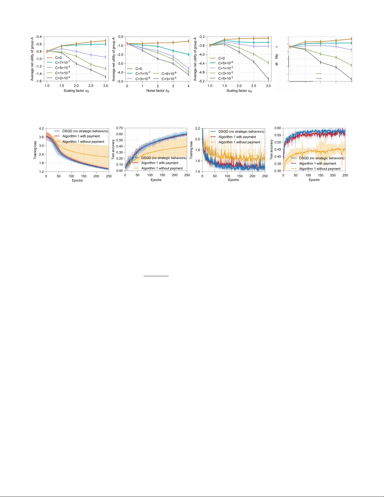
1 Gradient Manipulation in Distrib uted Stochastic Gradient Descent with Strate gic Agents: T ruthful Incenti v es with Con v er gence Guarantees Ziqin Chen and Y ongqiang W ang, Senior Member , IEEE Abstract —Distributed learning has gained signiﬁcant attention due to its advantages in scalability , priv acy , and fault tolerance. In this paradigm, multiple agents collaboratively train a global model by exchanging parameters only with their neighbors. Howev er , a key vulnerability of existing distributed learning approaches is their implicit assumption that all agents behave honestly during gradient updates. In real-world scenarios, this assumption often breaks down, as selﬁsh or strategic agents may be incentivized to manipulate gradients for personal gain, ulti- mately compromising the ﬁnal learning outcome. In this w ork, we propose a fully distributed payment mechanism that, for the ﬁrst time, guarantees both truthful behaviors and accurate conv er- gence in distributed stochastic gradient descent. This represents a signiﬁcant advancement, as it overcomes two major limitations of existing truthfulness mechanisms for collaborative learning: (1) reliance on a centralized server for payment collection, and (2) sacriﬁcing con vergence accuracy to guarantee truthfulness. In addition to characterizing the conv ergence rate under general con vex and strongly con vex conditions, we also prove that our approach guarantees the cumulative gain that an agent can obtain through strategic behavior remains ﬁnite, even as the number of iterations approaches inﬁnity—a pr operty unattainable by most existing truthfulness mechanisms. Our experimental results on standard machine learning tasks, evaluated on benchmark datasets, conﬁrm the effectiveness of the proposed approach. Index T erms —T ruthfulness, gradient manipulation, distributed stochastic gradient descent, strategic behavior . I . I N T RO D U C T I O N Recent years hav e witnessed signiﬁcant advances in dis- tributed methods for collaborati ve optimization and learn- ing [1]–[4]. By distributing both data and computational resources across multiple agents, distrib uted methods le ver- age the combined computing po wer of multiple devices to collaborativ ely train a global model without the need for a centralized server . Compared with server -assisted collaborativ e learning 1 , distributed learning av oids monopolistic control and single points of failure [5], and hence, is widely applied in areas such as distributed machine learning [6], multi-robot coordination [7], and wireless networks [8]. Howe ver , almost all existing distributed learning approaches implicitly assume that all participating agents act truthfully This work was supported by the National Science Foundation under Grant CCF-2106293, Grant CCF-2215088, Grant CNS-2219487, Grant CCF- 2334449, and Grant CNS-2422312. (Corresponding author: Y ongqiang W ang, email:yongqiw@clemson.edu). Ziqin Chen and Y ongqiang W ang are with the Department of Electrical and Computer Engineering, Clemson Univ ersity , Clemson, SC 29634 USA. 1 W e use “server-assisted collaborative learning” to refer to collaborative learning inv olving a centralized server or aggregator , with federated learning as a representative example. (see, e.g., [9]–[19]), which is essential for their success- ful ex ecution. This premise becomes untenable in practical scenarios where participating agents are strategic and self- interested. In such cases, participating agents may manipulate gradient updates to maximize their o wn utilities, ultimately undermining the performance of collaborativ e learning. For example, in distributed learning with heterogeneous data dis- tributions, an agent may inﬂate its local gradient updates to ske w the ﬁnal model in fav or of its own data distribution [20], [21]. Similarly , in a shared market, a ﬁrm may inject noise into its shared data to degrade the quality of other ﬁrms’ predictiv e model training, thereby maintaining competitiv e advantage [22]. More motiv ating examples are provided in Section II-B. Such untruthful beha viors pose a signiﬁcant threat to the performance of existing distributed learning and optimization algorithms (as demonstrated by our experimental results in Fig. 2). T o mitigate strategic behaviors of participating agents in collaborativ e learning, several approaches hav e been proposed, which can be broadly categorized into incentive-based ap- proaches [23]–[38] and joint-dif ferential-priv acy (JDP)-based approaches [39]–[42]. Howe ver , all existing approaches rely on a centralized server to collect information from all agents and then execute a truthfulness mechanism [34]. For example, the V ickrey–Clark e–Groves (VCG) mechanism [43]–[45], a well-known incentiv e-based approach, requires a centralized server to aggregate true gradients/functions from all agents to compute the corresponding monetary transfers. Similarly , JDP-based approaches require a centralized server to collect iteration variables from all agents in order to compute the necessary noise [39]–[42] 2 . T o the best of our knowledge, no existing approaches can effecti vely incentivize truthful behaviors in fully distributed optimization and learning. A. Related literatur e Incentive-based truthfulness approaches. T ruthfulness in statistical (mean) estimation has been addressed using incen- tiv e/payment mechanisms [24], [27], [29]. These mechanisms are typically one-shot, where agents choose their strate gies once and a centralized server broadcasts payments accordingly , 2 Although the recent work by [46] proposes a JDP-based truthfulness approach for distributed aggregative optimization, it is limited to scenarios where each agent’s objective function depends on an aggregati ve term of others’ optimization variables. Furthermore, due to differential-priv acy noise injection, the approach achiev es truthfulness at the cost of compromised optimization accuracy (see Theorem 3 in [46] for details). 2 which renders them inapplicable to multi-round, gradient- based distrib uted learning algorithms. Based on the well- known VCG mechanism [43]–[45], truthfulness results have also been reported for federated learning (see, e.g., [20]– [22], [32]–[35]). Howe ver , the VCG mechanism relies on a server to calculate and collect monetary payments, which makes it inapplicable in a fully distributed setting. Moreover , VCG-based approaches are not budget-balanced and often in volv e surplus payments [30]–[34], which further limits their practicality . It is worth noting that many results have discussed incentiv e mechanisms for encouraging agents’ contributions of data/resources in collaborativ e learning [24], [32], [33]. Howe ver , those results do not consider agents’ strategic ma- nipulation on iterative updates for personal gains. JDP-based truthfulness approaches. JDP-based approaches incentivize truthful behavior by injecting noise into algo- rithmic outputs, thereby masking the impact of any single agent’ s misreporting on the ﬁnal model and promoting truth- fulness [39]–[42]. Howe ver , these approaches require a cen- tralized server to collect local optimization variables from all agents to determine the needed noise amplitude, which makes it infeasible in a fully distrib uted setting. Moreover , JDP- based approaches hav e to compromise con vergence accuracy to ensure truthfulness [46], which is undesirable in accuracy- sensitiv e applications. T ABLE I C O MPA R IS O N O F O U R A P PR OAC H W I T H E XI S T I NG T RU T HF U L N ES S R E SU LT S F O R D I S TR I B UT E D O P T IM I Z A T I ON / L E AR N I N G . Approach Fully ε -Incentiv e Budget Accurate distributed? compatible? a balanced? b con vergence? [34] ✗ ✓ ✗ ✓ [22] ✗ ✗ ✓ ✗ [20], [21] ✗ ✗ ✓ ✗ [46] ✓ ✓ ✓ ✗ Our approach ✓ ✓ ✓ ✓ a W e use “ ε -Incentive compatible” to describe whether an approach can guarantee that the cumulati ve gain that an agent obtains from persistent strategic behaviors remains ﬁnite (bounded by some ﬁnite value ε ), ev en as the number of iterations approaches inﬁnity . b W e use “Budget balanced” to mean total payments collected equal total payments made, requiring no external subsidies or surplus. This ensures that the mechanism is ﬁnancially sustainable and scalable in practice. B. Contributions In this article, we propose a distributed payment mechanism that guarantees both truthful behavior of agents and accurate con vergence in distrib uted stochastic gradient methods. The main contributions are summarized as follows (T able I high- lights the contributions and their comparison with existing truthfulness results): • W e propose a fully distributed payment mechanism that incentivizes truthful behaviors among interacting strate gic agents in distributed stochastic gradient methods. This represents a substantial breakthrough, as existing truth- fulness mechanisms (in, e.g., [20]–[42]) all rely on a centralized server to aggregate local information from agents. T o the best of our knowledge, this is the ﬁrst payment mechanism for distributed gradient descent without the assistance of any centralized server . • Our payment mechanism guarantees that the incentiv e for a strategic agent to deviate from truthful beha viors diminishes to zero ov er time (see Lemma 1). Building on this, we further prov e that the cumulativ e gain that an agent can obtain from its strategic behaviors remains ﬁnite, ev en when the number of iterations tends to inﬁnity (see Theorem 2). This stands in sharp contrast to ex- isting incenti ve-based approaches for federated learning in [20]–[22], which cannot eliminate agents’ incentiv es to behave untruthfully–resulting in a cumulativ e gain that grows unbounded when the number of iterations tends to inﬁnity . • In addition to ensuring diminishing incenti ves for untruth- ful behavior in distributed gradient descent, our payment mechanism also guarantees accurate conv ergence, ev en in the presence of persistent gradient manipulation by agents (see Theorem 1). This is in stark contrast to existing JDP-based truthfulness results in [39]–[42], [46] and incentiv e-based truthfulness results in [20]–[22], all of which are subject to an optimization error . W e analyze the con vergence rates of distributed gradient descent under our payment mechanism for general con vex and strongly con vex objecti ve functions. This is more comprehensive than existing truthfulness results in [20]–[22], [34] that focus solely on the strongly con vex case. • Different from most existing VCG-based approaches (in, e.g., [30]–[34]), which cannot ensure budget-balance (the total payments from all agents sum to zero, a property essential for the ﬁnancial sustainability and practical scalability of the mechanism), our payment mechanism is budget-balanced. This is signiﬁcant in a fully distributed setting since no centralized server is used to manage subsidies or surplus. • W e ev aluate the performance of our truthful mechanism using representative distributed learning tasks, including image classiﬁcation on the FeMNIST dataset and next- character prediction on the Shakespeare dataset. The experimental results conﬁrm the ef fectiv eness of our approach. The organization of the paper is as follows. Sec. II intro- duces the problem formulation, presents motivating examples, and formalizes the used game-theoretic framework. Sec. III proposes the distrib uted payment mechanism. Sec. IV analyzes con vergence rate and establishes incenti ve compatibility guar- antees. Sec. V presents experimental results. Finally , Sec. VI concludes the paper . Notations: W e use R n to denote the set of n -dimensional real Euclidean space. W e denote ∇ F ( θ ) as the gradient of F ( θ ) and E [ θ ] as the expected value of a random variable θ . W e denote the set of N agents by [ N ] and the neighboring set of agent i as N i . The cardinality of N i is denoted as deg ( i ) . W e denote the coupling matrix by W = { w ij } ∈ R N × N , where w ij > 0 if agent j interacts with agent i , and w ij = 0 otherwise. W e deﬁne w ii = 1 − P j ∈N i w ij . W e abbreviate “with respect to” as w .r .t. Furthermore, we use an overbar to denote the av erage of all agents, e.g., ¯ θ t = 1 N P N i =1 θ i,t , and use bold font with iteration subscripts to denote the stacked 3 vector of all N agents, e.g., θ t = col( θ 1 ,t , · · · , θ N ,t ) . I I . P RO B L E M F O R M U L A T I O N A N D P R E L I M I NA R I E S A. Distributed optimization and learning W e consider N ≥ 2 agents participating in distributed optimization and learning, each possessing a priv ate dataset whose distribution can be heterogeneous across the agents. The goal is for all agents to cooperatively ﬁnd a solution θ ∗ to the following stochastic optimization problem: min θ ∈ R n F ( θ ) = 1 N N X i =1 f i ( θ ) , f i ( θ ) = E ζ i ∼P i [ l ( θ ; ζ i )] , (1) where θ ∈ R n denotes a global model parameter and ζ i is a random data sample of agent i drawn from its local data distribution P i . The loss function l ( θ ; ζ i ) : R n × R n 7→ R is assumed to be dif ferentiable in θ for ev ery ζ i and the local objectiv e function f i ( θ ) of agent i can be noncon vex. In real-world applications, the data distribution P i is typi- cally unkno wn. Hence, each agent i can only access a noisy estimate of the gradient ∇ f i ( θ i,t ) , computed at its current local model parameter θ i,t using the a vailable local data. For example, at each iteration t , agent i samples a batch of B ≥ 1 data points and computes a gradient estimate as g i ( θ i,t ) = 1 B P B j =1 ∇ l ( θ i,t ; ζ ij ) . Using this gradient estimate g i ( θ i,t ) , along with the model parameters { θ j,t } j ∈N i receiv ed from its neighbors, agent i updates its local parameter accord- ing to a distributed optimization/learning algorithm. Existing distributed optimization/learning algorithms (see, e.g., [9]–[19]) uni versally assume that participating agents are honest and behave truthfully . Howe ver , this assumption may be unrealistic in real-world scenarios, where agents can beha ve selﬁshly or strategically . For example, a strategic agent may amplify its gradient estimates to bias the ﬁnal model parameter in fav or of its own data distribution, or inject noise into its gradient information to degrade the performance of other agents’ models for competiti ve advantage. (W e provide addi- tional motiv ating examples to illustrate ho w agents can beneﬁt from gradient manipulation in distributed least squares and distributed mean estimation in Section II-B.) Such strategic gradient manipulation can signiﬁcantly degrade the learning performance of existing distributed learning algorithms (as evidenced by our experimental results in Fig. 2). Next, we discuss the classical Distributed Stochastic Gra- dient Descent (Distributed SGD) in the presence of gradient manipulation by a strategic agent i ∈ [ N ] . Distributed SGD in the pr esence of strategic behavior . At each iteration t , each agent i strate gically chooses a manipulated gradient m i,t , which, in general, is a function of agent i ’ s true gradient g i ( θ i,t ) . Using the manipulated gradient m i,t and the model parameters { θ j,t } j ∈N i receiv ed from its neighbors, each agent i updates its local model parameter according to Algorithm 1. Algorithm 1 Distributed SGD in the presence of strategic behavior (from agent i ’ s perspectiv e) 1: Initialization: θ i, 0 ∈ R n ; stepsize λ t > 0 . 2: Send θ i, 0 to neighbors j ∈ N i and recei ve θ j, 0 from neighbors j ∈ N i . 3: for t = 0 , . . . , T do 4: θ i,t +1 = P j ∈N i ∪{ i } w ij θ j,t − λ t m i,t ; 5: Send θ i,t +1 to neighbors j ∈ N i and recei ve θ j,t +1 from neighbors j ∈ N i . 6: end for It is worth noting that we focus on gradient manipulation rather than model-parameter manipulation for two reasons. First, any manipulation of model parameters shared among agents effecti vely corresponds to some form of alteration in the gradient estimates, as proven in Corollary 1 in Appendix E. Second, gradient manipulation is the most direct and practically effecti ve strategy for a strategic agent to increase its personal gain. Speciﬁcally , by upscaling its o wn gradient estimates, an agent can increase the inﬂuence of its local data on the cooperativ e learning process, thereby pulling the ﬁnal model parameter closer to the minimizer of its local objectiv e function and reducing its own cost. On the other hand, by injecting noise into its gradient estimates, an agent can reduce the usefulness of its data to its neighbors, degrading their model performance and gaining competiti ve advantage. In comparison, manipulating model parameters does not provide a clear strategic beneﬁt. For these reasons, we focus on gradient manipulation as the primary form of untruthful or strategic behavior of participating agents. B. Motivating examples In this subsection, we ﬁrst use a distributed least-squares problem to show that strategic agents can lo wer their individual costs by amplifying local gradients, at the expense of network performance. W e then consider a distributed mean estimation problem with stochastic gradients to sho w that agents can further improv e their payoffs by manipulating gradient updates in Algorithm 1, again sacriﬁcing network performance. Example 1 (Distributed least squares) . W e consider a distributed least squares problem where N agents coopera- tiv ely ﬁnd an optimal solution θ ∗ to the following stochastic optimization problem: min θ ∈ R n F ( θ ) = 1 N P N i =1 f i ( θ ) , f i ( θ ) = E [( u ⊤ i θ − v i ) 2 ] , (2) where u i ∈ R n denotes a feature vector that is independently and identically drawn from an unknown distribution with zero mean and a positiv e deﬁnite cov ariance matrix, i.e., E [ u i ] = 0 and E [ u i u ⊤ i ] = Σ ≻ 0 . The label v i ∈ R is generated according to the linear model v i = u ⊤ i z i + ξ i , where z i represents agent i ’ s predeﬁned local target and ξ i denotes zero-mean noise independent of u i and has a variance of σ 2 ξ . The gradient of the global objecti ve function satisﬁes g ( θ ) = 1 N P N i =1 2 E [ u i u ⊤ i ]( θ − z i ) = 2Σ ( θ − ¯ z ) , which implies that the optimal solution is θ ∗ = ¯ z . 4 T o study the effect of gradient manipulation, we assume that agent i deviates from truthful behavior by amplifying its gradients g i ( θ ) = 2Σ( θ − z i ) by a scalar a i > 1 , while all other agents behav e truthfully . Then, the gradient of the global objectiv e function becomes g ′ ( θ ) = 2Σ  ( a i + N − 1) θ N − a i z i + P N j  = i z j N  , which leads to a new optimal solution at θ ′∗ = a i − 1 a i + N − 1 z i + N a i + N − 1 ¯ z with any a i > 1 . Using the expressions for θ ∗ and θ ′∗ , we have ∥ θ ′∗ − z i ∥ = N a i + N − 1 ∥ ¯ z − z i ∥ < ∥ ¯ z − z i ∥ = ∥ θ ∗ − z i ∥ , which implies that the optimal solution θ ′∗ is closer to agent i ’ s local target z i (and is also closer to agent i ’ s local optimum θ ∗ i due to θ ∗ i = z i ) than the original optimal solution θ ∗ . Moreov er, a lar ger a i makes θ ′∗ closer to z i . Therefore, agent i achieves a lo wer cost: f i ( θ ′∗ ) =  N a i + N − 1  2 ( ¯ z − z i ) ⊤ Σ( ¯ z − z i ) + σ 2 ξ < ( ¯ z − z i ) ⊤ Σ( ¯ z − z i ) + σ 2 ξ = f i ( θ ∗ ) , while the global objectiv e function value is increased to F ( θ ′∗ ) = F ( θ ∗ ) +  a i − 1 a i + N − 1  2 ( z i − ¯ z ) ⊤ Σ( z i − ¯ z ) , which implies that by amplifying its local gradients (i.e., by using a i > 1 ), a strategic agent i can reduce its individual cost while increasing the global objectiv e function v alue. Example 2 (Consensus-based distributed mean estimation) . W e consider a problem where N agents cooperativ ely estimate a global mean µ = 1 N P N i =1 µ i , where µ i ∈ R n denotes the mean of agent i ’ s data distribution. Formally , the distributed mean estimation problem can be formulated as the following stochastic optimization problem: min θ ∈ R n F ( θ ) = 1 N P N i =1 f i ( θ ) , f i ( θ ) = E [ ∥ θ − µ i ∥ 2 ] . (3) W e assume that the agents cooperatively solve problem (3) using Algorithm 1 with a diminishing stepsize λ t = λ 0 ( t +1) v , where λ 0 < 1 2 and 0 < v < 1 . Since the mean µ i is typically unknown to agent i , the agent only has access to a noisy gradient estimate g i ( θ i,t ) = 2( θ i,t − ζ i,t ) at iteration t , based on a sample ζ i,t from its local distribution. Speciﬁcally , each coordinate ζ p i,t , p ∈ [ n ] of ζ i,t is independently sampled from N ( µ p i , σ 2 /n ) . W e denote µ i = col( µ 1 i , · · · , µ n i ) and the mean squared error of agent i as lim T →∞ f i ( ¯ θ T ) = lim T →∞ = E [ ∥ ¯ θ T − µ i ∥ 2 ] . Next, we prov e that by amplifying its gradient estimates with a i > 1 , strategic agent i can reduce its mean squared error by a factor of ( N a i + N − 1 ) 2 , while increasing the global mean squared error by an additive term of  a i − 1 a i + N − 1  2 ∥ µ − µ i ∥ 2 . 1) W e ﬁrst consider the case where all agents are truthful. Algorithm 1 with m i,t = g i ( θ i,t ) implies ¯ θ t +1 − µ = (1 − 2 λ t )( ¯ θ t − µ ) + 2 λ t ( ¯ ζ t − µ ) . By using relations E [ ¯ ζ t ] = µ and E [ ∥ ¯ ζ t − µ ∥ 2 ] ≤ σ 2 N , and the fact that ¯ ζ t − µ is independent of ¯ θ t − µ , we hav e E [ ∥ ¯ θ t +1 − µ ∥ 2 ] = (1 − 2 λ t ) 2 E [ ∥ ¯ θ t − µ ∥ 2 ] + 4 λ 2 t σ 2 N . (4) By applying Lemma 5-(i) in the arxiv version of [46] to (4), we obtain E [ ∥ ¯ θ t − µ ∥ 2 ] ≤ c 1 λ t , with c 1 = 1 λ 0 max n E [ ∥ ¯ θ 0 − µ ∥ 2 ] , 4 λ 2 0 σ 2 N (2 λ 0 − v ) o . Using the relation E [ ∥ a + b ∥ 2 ] ≤ ( p E [ ∥ a ∥ 2 ] + p E [ ∥ b ∥ 2 ]) 2 for any random variables a and b , we hav e E [ ∥ ¯ θ t − µ i ∥ 2 ] ≤  p E [ ∥ ¯ θ t − µ ∥ 2 ] + p E [ ∥ µ − µ i ∥ 2 ]  2 ≤  √ c 1 λ t + ∥ µ − µ i ∥  2 , (5) which implies lim T →∞ E [ ∥ ¯ θ T − µ i ∥ 2 ] ≤ ∥ µ − µ i ∥ 2 . In addition, combining the relationship (1 − 2 λ t ) 2 ≥ 1 − 4 λ t and (4), we have E [ ∥ ¯ θ t +1 − µ i ∥ 2 ] ≥ (1 − 4 λ t ) E [ ∥ ¯ θ t − µ i ∥ 2 ] + 4 λ 2 t σ 2 N , (6) which further implies E [ ∥ ¯ θ t − µ i ∥ 2 ] ≥ c 2 λ t , with c 2 = 1 λ 0 min n E [ ∥ ¯ θ 0 − µ i ∥ 2 ] , 2 λ 0 σ 2 N o . Using the inequality E [ ∥ a + b ∥ 2 ] ≥ ( p E [ ∥ a ∥ 2 ] − p E [ ∥ b ∥ 2 ]) 2 for any random variables a and b , we hav e E [ ∥ ¯ θ t − µ i ∥ 2 ] ≥  √ c 2 λ t − ∥ µ − µ i ∥  2 , (7) which implies lim T →∞ E [ ∥ ¯ θ T − µ i ∥ 2 ] ≥ ∥ µ − µ i ∥ 2 . Combining (5) and (7), and using lim T →∞ λ T = 0 yield lim T →∞ f i ( ¯ θ T ) = lim T →∞ E [ ∥ ¯ θ T − µ i ∥ 2 ] = ∥ µ − µ i ∥ 2 , (8) while the global mean squared error satisﬁes lim T →∞ F ( ¯ θ T ) = 1 N P N j =1 ∥ µ − µ j ∥ 2 . (9) 2) Next, we consider the case where agent i ampliﬁes its gradient estimates as a i g i ( θ ′ i,t ) = 2 a i ( θ ′ i,t − ζ i,t ) , while all other agents behav e truthfully . According to Algorithm 1, we hav e the following dynamics ¯ θ ′ t +1 = ¯ θ ′ t − 2( a i + N − 1) N λ t  ¯ θ ′ t −  a i ζ i,t + P N j  = i ζ j,t a i + N − 1  − 2( a i − 1) N λ t ( θ ′ i,t − ¯ θ ′ t ) . (10) For the sake of notational simplicity , we deﬁne ˆ a i ≜ a i + N − 1 N and ˆ µ i ≜ a i µ i + P N j  = i µ j a i + N − 1 . Then, by using (10), we obtain ¯ θ ′ t +1 − ˆ µ i = (1 − 2 ˆ a i λ t )  ¯ θ ′ t − ˆ µ i  + 2ˆ a i λ t  a i ζ i,t + P N j  = i ζ j,t a i + N − 1 − ˆ µ i  − 2( a i − 1) N λ t ( θ ′ i,t − ¯ θ ′ t ) . (11) By taking the squared norm and expectations on both sides of (11) and using the Y oung’ s inequality , we obtain E [ ∥ ¯ θ ′ t +1 − ˆ µ i ∥ 2 ] = (1 + ˆ a i λ t ) E [ ∥ (1 − 2ˆ a i λ t )  ¯ θ ′ t − ˆ µ i  ∥ 2 ] +  1 + 1 ˆ a i λ t  E     2( a i − 1) λ t N ( θ ′ i,t − ¯ θ ′ t )    2  + 4ˆ a 2 i λ 2 t ( a 2 i + N − 1) σ 2 ( a i + N − 1) 2 , ≤ (1 − ˆ a i λ t ) E [ ∥ ¯ θ ′ t − ˆ µ i ∥ 2 ] + 4ˆ a 2 i ( a 2 i + N − 1) σ 2 ( a i + N − 1) 2 λ 2 t +  λ 0 + 1 ˆ a i  4( a i − 1) 2 N 2 λ t E [ ∥ θ ′ i,t − ¯ θ ′ t ∥ 2 ] . (12) 5 Furthermore, Algorithm 1 with m i,t = 2 a i ( θ ′ i,t − ζ i,t ) and the dynamics in (10) imply θ ′ t +1 − 1 N ⊗ ¯ θ ′ t +1 = ( W ⊗ I n )  θ ′ t − 1 N ⊗ ¯ θ ′ t  − 2 λ t  θ ′ t − 1 N ⊗ ¯ θ ′ t −  ζ t − 1 N ⊗ ¯ ζ t  + 2 λ t M i ( θ ′ i,t − ζ i,t ) , (13) where matrix M i is gi ven by M i = (1 − a i )( e i − 1 N 1 N ) ⊗ I n with e i ∈ R N denoting the i th standard basis vector . By taking the squared norm and expectations on both sides of (13) and using the Y oung’ s inequality , we obtain E [ ∥ θ ′ t +1 − 1 N ⊗ ¯ θ ′ t +1 ∥ 2 ] ≤ (1 + (1 − ρ )) E [ ∥ ( W ⊗ I n − 2 λ t I N n )( θ ′ t − 1 N ⊗ ¯ θ ′ t ) ∥ 2 ] + 8 λ 2 t  1 + 1 1 − ρ  E [ ∥ ζ t − 1 N ⊗ ¯ ζ t ∥ 2 ] + 8 λ 2 t  1 + 1 1 − ρ  ∥ M i ∥ 2 E [ ∥ θ ′ i,t − ζ i,t ∥ 2 ] . (14) The last term on the right hand side of (14) satisﬁes E [ ∥ θ ′ i,t − ζ i,t ∥ 2 ] ≤ 3 E [ ∥ θ ′ i,t − ¯ θ ′ t ∥ 2 ] + 3 E [ ∥ ¯ θ ′ t − ˆ µ i ∥ 2 ] + 3 E [ ∥ ˆ µ i − ζ i,t ∥ 2 ] . (15) Substituting (15) into (14), we obtain E [ ∥ θ ′ t +1 − 1 N ⊗ ¯ θ ′ t +1 ∥ 2 ] ≤  ( ρ − 2 λ t ) 2 ρ + 24(2 − ρ ) ∥ M i ∥ 2 1 − ρ λ 2 t  E [ ∥ θ ′ t − 1 N ⊗ ¯ θ ′ t ∥ 2 ] + 24(2 − ρ ) ∥ M i ∥ 2 1 − ρ λ 2 t  E [ ∥ ¯ θ ′ t − ˆ µ i ∥ 2 ] + E [ ∥ ˆ µ i − ζ i,t ∥ 2 ]  + 8(2 − ρ ) 1 − ρ λ 2 t E [ ∥ ζ t − 1 N ⊗ ¯ ζ t ∥ 2 ] , (16) where in the deri vation we ha ve used the relations 1+ (1 − ρ ) ≤ 1 ρ and E [ ∥ θ ′ i,t − ¯ θ ′ t ∥ 2 ] ≤ E [ ∥ θ ′ t − 1 N ⊗ ¯ θ ′ t ∥ 2 ] . Summing both sides of (12) and (16), we arriv e at E [ ∥ ¯ θ ′ t +1 − ˆ µ i ∥ 2 ] + E [ ∥ θ ′ t +1 − 1 N ⊗ ¯ θ ′ t +1 ∥ 2 ] ≤  1 − ˆ a i λ t + 24(2 − ρ ) ∥ M i ∥ 2 1 − ρ λ 2 t  E [ ∥ ¯ θ ′ t − ˆ µ i ∥ 2 ] +  ( ρ − 2 λ t ) 2 ρ + 4( λ 0 ˆ a i +1)( a i − 1) 2 ˆ a i N 2 λ t + 24(2 − ρ ) ∥ M i ∥ 2 1 − ρ λ 2 t  × E [ ∥ θ ′ t − 1 N ⊗ ¯ θ ′ t ∥ 2 ] + c i, 1 λ 2 t , with c i, 1 = 4ˆ a 2 i ( a 2 i + N − 1) σ 2 ( a i + N − 1) 2 + 24(2 − ρ ) ∥ M i ∥ 2 P N j =1 ∥ µ j − µ i ∥ 2 1 − ρ + 24(2 − ρ ) ∥ M i ∥ 2 σ 2 (1 − ρ )( a i + N − 1) + 32(2 − ρ ) d 2 ζ 1 − ρ and d ζ = max i ∈ [ N ] ,t ∈ N {∥ ζ i,t ∥} . Since λ t is a decaying sequence, we hav e E [ ∥ ¯ θ ′ t +1 − ˆ µ i ∥ 2 ] + E [ ∥ θ ′ t +1 − 1 N ⊗ ¯ θ ′ t +1 ∥ 2 ] ≤  1 − ˆ a i λ t 2   E [ ∥ ¯ θ ′ t − ˆ µ i ∥ 2 ] + E [ ∥ θ ′ t − 1 N ⊗ ¯ θ ′ t ∥ 2 ]  + c i, 1 λ 2 t . Applying Lemma 5-(i) in the arxiv version of [46] to the preceding inequality , we arrive at E [ ∥ ¯ θ ′ t − ˆ µ i ∥ 2 ] + E [ ∥ θ ′ t − 1 N ⊗ ¯ θ ′ t ∥ 2 ] ≤ c i, 2 λ t , (17) with c i, 2 = max { E [ ∥ ¯ θ 0 − ˆ µ ∥ 2 ] + E [ ∥ θ 0 − 1 N ⊗ ¯ θ 0 ∥ 2 ] , 2 c i, 1 λ 2 0 ˆ a i λ 0 − 2 v } . By using E [ ∥ a + b ∥ 2 ] ≤ ( p E [ ∥ a ∥ 2 ] + p E [ ∥ b ∥ 2 ]) 2 for any random variables a and b , we have E [ ∥ ¯ θ ′ t − µ i ∥ 2 ] ≤  p E [ ∥ ¯ θ ′ t − ˆ µ i ∥ 2 ] + p E [ ∥ ˆ µ i − µ i ∥ 2 ]  2 ≤  p c i, 2 λ t +  N a i + N − 1  ∥ µ − µ i ∥  2 , which implies that agent i obtains a lower mean-squared error: lim T →∞ f i ( ¯ θ ′ T ) =  N a i + N − 1  2 ∥ µ − µ i ∥ 2 < ∥ µ − µ i ∥ 2 = lim T →∞ f i ( ¯ θ T ) , (18) while the global mean-squared error is increased to lim T →∞ F ( ¯ θ ′ T ) = lim T →∞ 1 N P N j =1 E [ ∥ ¯ θ ′ t − µ j ∥ 2 ] ≤ lim T →∞ 1 N P N j =1  p c i, 2 λ t + p E [ ∥ ˆ µ i − µ j ∥ 2 ]  2 ≤ 1 N P N j =1 ∥ ( a i − 1)( µ i − µ ) a i + N − 1 + µ − µ j ∥ 2 = 1 N P N j =1 ∥ µ − µ j ∥ 2 +  a i − 1 a i + N − 1  2 ∥ µ − µ i ∥ 2 = lim T →∞ F ( ¯ θ T ) +  a i − 1 a i + N − 1  2 ∥ µ − µ i ∥ 2 . (19) Example 1 and Example 2 demonstrate that a self-interested agent can beneﬁt from its strategic gradient manipulation while degrading the network-le vel performance. In addition to decentralized least squares problems, similar truthfulness issues also emerge in collaborative machine learn- ing [22], distributed electric-vehicle charging [46], and many other collaborative optimization applications [38]. T o quantitativ ely analyze strategic interactions among agents, we adopt a game-theoretic frame work that explicitly deﬁnes each agent’ s strategic behavior , rew ard, payment, and resulting net utility . C. Game-theor etic framework Strategic behaviors and action space. A self-interested agent can enhance its individual outcome through two strate gic behaviors: amplifying its gradient estimates to bias the ﬁnal model parameter in fav or of its own data distribution, and injecting noise to degrade the performance of other agents’ model parameters for competitiv e advantage. Both strategic behaviors can be modeled as an agent’ s action at each iteration. Formally , we deﬁne the action space for each strategic agent i ∈ [ N ] in distributed optimization/learning as follo ws: A i = { α i | α i ( g i ( θ )) = a i g i ( θ ) + b i ξ i , a i ≥ 1 , b i ∈ R } , (20) where g i ( θ ) represents agent i ’ s true gradient estimate and ξ i is a zero-mean noise vector with bounded variance. The scaling factor a i quantiﬁes the degree of gradient ampliﬁcation, while the noise factor b i speciﬁes the magnitude of noise injection, both of which can be strategically chosen by agent i at each iteration. For any action space A i , we assume that it includes the identity mapping, which maps g i to itself with probability one. Hence, truthfulness is always a feasible action. The action space deﬁned in (20) is designed to capture the strategic behavior of agents in distributed learning rather than arbitrary malicious attacks. T o this end, we consider a i ≥ 1 and ignore a i < 1 , because the latter typically reduces the inﬂuence of agent i ’ s local data on cooperative learning, mak- ing it a non-utility-improving choice for a rational agent. This focus on strategic, utility-driv en behavior excludes general malicious attacks, which are typically disruptiv e and do not align with an agent’ s goal of improving its outcome within the learning framew ork. In addition, compared with the action 6 spaces deﬁned in existing results on federated learning, such as [22] that only considers noise injection (i.e., ﬁxing a i = 1 ) and [20] that only considers gradient ampliﬁcation (i.e., ﬁxing b i = 0 ), our formulation accounts for a broader range of strategic manipulations. Rewards. W e denote a distributed learning algorithm as M . At each iteration t , agent i chooses an action α i,t ∈ A i . This action produces a (manipulated) gradient m i,t = α i,t ( g i ( θ i,t )) , which is then used by agent i in the update step of M . Considering T + 1 iterations of M , we let α i = { α i,t } T t =0 denote the action trajectory of agent i from iteration 0 to iteration T , θ j = { θ j,t } T t =0 denote the model-parameter trajectory of agent j , and θ − i = { θ j } j ∈N i denote the collection of model-parameter trajectories recei ved by agent i from all its neighbors. Gi ven an initial model parameter θ i, 0 , an action trajectory α i , and a collection of model-parameter trajectories θ − i , an implementation of M generates a ﬁnal model parameter θ i,T +1 = M ( θ i, 0 , α i , θ − i ) for agent i . W e denote the reward that agent i obtains from its ﬁnal objectiv e (cost) function value as R i ( f i ( θ i,T +1 )) . In a minimization problem (see (1)), the reward function R i ( f i ( θ )) increases as the objective function f i ( θ ) decreases. Therefore, a self-interested agent can boost its rew ard by biasing the ﬁnal solution to ward the minimizer of its local objectiv e function. Common choices for R i ( f i ( θ )) include the linear function R i ( f i ( θ )) = − f i ( θ ) and the sigmoid-like function R i ( f i ( θ )) = (1+ e − 1 /f i ( θ ) ) − 1 [21]. W e allo w different agents to have different rew ard functions. Payments and net utilities. T o mitigate gradient manipulation by participating agents, we augment the distributed learning protocol with a payment mechanism. This mechanism can be computed efﬁciently and implemented in a fully decentralized manner between any pair of interacting agents (see details in Section III). W e denote the augmented distributed learning protocol (with a payment mechanism) by M p . The net utility of agent i from executing M p ov er T + 1 iterations is deﬁned as follows: U M p i, 0 → T ( α i , α − i ) = R i ( f i ( θ i,T +1 )) − T X t =0 P i,t , (21) where P i,t is the total net payment made by agent i to all its neighbors, and α − i = { α j } j  = i denotes the action trajectories of all agents except agent i . W e note that all existing incentiv e-based approaches for collaborativ e learning ensure truthfulness by incorporating a payment or penalty term into each agent’ s net utility . W ithout such payments, a self-interested agent can freely manipulate its gradients to reduce its o wn loss and increase its rewards, thereby distorting the collaborativ e learning process. There- fore, (21) includes the cumulativ e payments of each agent in its net utility . Accordingly , a rational agent must consider both its rewards and payments when maximizing its net utility . Next, we introduce two truthfulness-related concepts in our game-theoretic framework. Deﬁnition 1 ( δ -truthful action [20], [21]) . F or any given δ ≥ 0 and any i ∈ [ N ] , an action α i ∈ A i (with A i deﬁned in (20) ) of agent i is δ -truthful if it satisﬁes E [ ∥ α i ( g i ( θ )) − g i ( θ ) ∥ ] ≤ δ for any θ ∈ R n . In particular , the action α i is fully truthful when δ = 0 . Deﬁnition 1 quantiﬁes the truthfulness of an agent’ s action in collaborative optimization/learning. It can be seen that a smaller δ corresponds to a higher lev el of truthfulness in the agent’ s action. Deﬁnition 2 ( ε -incentiv e compatibility [47]) . F or any given ε ≥ 0 , a distrib uted learning pr otocol M p is ε -incentive compatible if for all i ∈ [ N ] , E [ U M p i, 0 → T ( h i , h − i )] ≥ E [ U M p i, 0 → T ( α i , h − i )] − ε holds for any arbitrary action trajec- tory α i of agent i , wher e h i is the truthful action trajectory of agent i and h − i is truthful action trajectories of all agents except agent i . Deﬁnition 2 (also called ε -Bayesian-incenti ve compatibility) is a standard and commonly used notion in the existing incentiv e-compatibility literature [20], [21], [48], [49]. It im- plies that if a distributed optimization protocol is ε -incentiv e compatible, then the expected net utility that an agent can gain from any (possibly untruthful) action trajectory is at most ε greater than that obtained by being truthful in all iterations. Clearly , a smaller ε corresponds to a lower gain that an untruthful agent can obtain. In addition, according to the deﬁnition of ε -Nash equilibrium in [50], if a distributed learning protocol is ε -incentiv e compatible, then the truthful action trajectory proﬁle of all agents h = ( h i , h − i ) forms an ε -Nash equilibrium (see Lemma 6 in Appendix E). I I I . P A Y M E N T M E C H A N I S M D E S I G N F O R D I S T R I B U T E D S T O C H A S T I C G R A D I E N T D E S C E N T In this section, we propose a fully distrib uted payment mechanism (see Mechanism 1) to incenti vize truthful behav- iors of participating agents in distributed stochastic gradient descent. Mechanism 1 Fully distributed payment mechanism (for interacting agents i and j at iteration t ) 1: Input: θ ι,t − 1 , θ ι,t , θ ι,t +1 for ι ∈ { i, j } av ailable to both agents i and j under Algorithm 1 (note θ ι,t +1 has been shared at the end of iteration t ); initialization θ i, − 1 = θ j, − 1 = 0 n ; C t > 0 . 2: Agents i and j simultaneously compute both ∆ θ i ,t ≜ ∥ θ i,t +1 − 2 θ i,t + θ i,t − 1 ∥ 2 and ∆ θ j ,t ≜ ∥ θ j,t +1 − 2 θ j,t + θ j,t − 1 ∥ 2 . 3: if ∆ θ i ,t ≥ ∆ θ j ,t then 4: Agent i transfers P j i,t = C t (∆ θ i ,t − ∆ θ j ,t ) to agent j . 5: else 6: Agent i receiv es P i j,t = C t (∆ θ j ,t − ∆ θ i ,t ) from agent j . 7: end if Mechanism 1 is implementable in a fully distributed manner without the assistance of any server or aggregator . At each iteration t , if agent i manipulates its gradient estimates such that its model-parameter increment ∥ θ i,t +1 − 2 θ i,t + θ i,t − 1 ∥ exceeds that of its neighbor agent j , agent i pays an amount P j i,t > 0 to agent j (in this case, we denote the payment 7 of agent j as P i j,t = − P j i,t ) . Con versely , if agent i ’ s model- parameter increment ∥ θ i,t +1 − 2 θ i,t + θ i,t − 1 ∥ is no greater than that of its neighbor agent j , it receiv es a payment of amount P i j,t ≥ 0 from agent j (in this case, we denote the payment of agent i as P j i,t = − P i j,t ). W e emphasize that our payment mechanism can be readily applied to any ﬁrst-order distributed gradient methods. For an agent i , its total payment to all its neighbors at iteration t is gi ven by P i,t = P j ∈N i P j i,t . In Mechanism 1, with both agents i and j ha ving ac- cess to θ ι,t − 1 , θ ι,t , and θ ι,t +1 for ι ∈ { i, j } from the update of Algorithm 1 (note that θ ι,t +1 has been shared at the end of iteration t ), the two agents can cross-verify the computed payment v alue, making the mechanism rob ust to unilateral manipulation. This represents a signiﬁcant advance compared with the payment mechanism in [34] for serv er- assisted collaborativ e optimization, which requires all agents to truthfully report their local objectiv e-function v alues for payment calculation—thereby creating a risk that strategic agents may manipulate the algorithmic update and the payment mechanism separately . Our payment mechanism can effecti vely discourage agents from free-riding 3 . Speciﬁcally , the model-parameter increment ∥ θ i,t +1 − 2 θ i,t + θ i,t − 1 ∥ of agent i depends on both the consensus errors and the (sign-indeﬁnite) local gradients. Con- sequently , e ven if agent i uses a zero (or lo w) gradient, there is no guarantee that ∥ θ i,t +1 − 2 θ i,t + θ i,t − 1 ∥ will be smaller than that of its neighbor j , meaning that lev eraging zero gradients does not reliably increase agent i ’ s payment gains. In fact, free- riding behavior (or using lo w gradients) in variably degrades agent i ’ s own reward R i ( f i ( θ i,T )) , as it weakens the inﬂuence of agent i ’ s data in collaborative learning and ultimately leads to a worse ﬁnal model for the agent itself. Hence, free-riding is not a utility-improving choice for a rational agent. Our payment mechanism is conceptually inspired by the classical VCG mechanism [43]–[45] but has sev eral funda- mental dif ferences: 1) conv entional VCG mechanisms require a central server to calculate and collect payments [43]–[45], whereas our mechanism operates in a pairwise fashion without reliance on any third party . As a result, it can be implemented in a fully distributed manner; 2) conv entional VCG mecha- nisms are typically designed for one-shot games [23], [25], [26], [28]. In contrast, our payment mechanism is naturally compatible with iterativ e algorithms, encompassing a wide range of distributed optimization/learning methods. In fact, an iterati ve algorithm setting inherently forms a multi-stage game, where agents repeatedly adjust actions, posing chal- lenges for both truthfulness and con vergence analysis; and 3) con ventional VCG mechanisms are not budget-balanced (see, e.g., [30]–[34]), whereas our payment mechanism is budget- balanced, i.e., P N i =1 P i,t = 0 , making it ﬁnancially sustainable and scalable in practice. The existing approaches most closely related to ours are the payment mechanisms proposed by [20], [21]. Howe ver , there are se veral fundamental differences: 1) our payment 3 Free-riding refers to the behavior in which agents skip computing gradients on their local data and instead update their parameters solely based on infor- mation received from neighbors. In this way , they beneﬁt from the distributed optimization process without contributing their own data or gradients. mechanism is implementable in a fully distributed manner , and hence, is applicable to arbitrary connected communication graphs, whereas the mechanisms in [20], [21] rely on a cen- tralized server to aggregate gradients from all agents, and thus operate only under a centralized communication structure; and 2) our payment mechanism achiev es ε -incentiv e compatibility with a ﬁnite ε e ven in an inﬁnite time horizon (see Theorem 2), whereas the incentiv e ε in [20], [21] becomes unbounded as the number of iterations tends to inﬁnity (see Claim 23 in [20] or Theorem 5.1 in [21]), leading to a v anishing incenti ve compatibility guarantee over iterations. I V . C O N V E R G E N C E R A T E A N D I N C E N T I V E - C O M P AT I B I L IT Y A NA LY S I S Assumption 1. F or any i ∈ [ N ] , the following conditions hold: (i) R i ( f i ( θ )) is L R,i -Lipschitz continuous w .r .t. θ ; (ii) the stoc hastic gradient g i ( θ ) is H i -Lipschitz continuous. Mor e- over , g i ( θ ) is unbiased and has bounded variance σ 2 i ; (iii) for a general conve x f i ( θ ) , we assume that f i ( θ ) is L f ,i -Lipschitz continuous. However , this assumption is not r equir ed for a str ongly con vex f i ( θ ) . Assumption 2. W e assume that the matrix W is symmetric and ρ = max {| π 2 | , | π N |} < 1 , wher e π N ≤ · · · ≤ π 2 < π 1 = 1 denote the eigen values of W . Assumption 1 is standard and commonly used in the dis- tributed stochastic optimization/learning literature [51]–[53]. It is worth noting that we allow f i ( θ ) to be conv ex, which is more general than the strongly conv ex assumption used in existing truthfulness results in [20]–[22], [34], [39]. Assump- tion 2 ensures that the communication graph is connected [54]. Furthermore, for the sake of notational simplicity , we de- note L R = max i ∈ [ N ] { L R,i } , L f = max i ∈ [ N ] { L f ,i } , H = max i ∈ [ N ] { H i } , and σ = max i ∈ [ N ] { σ i } . A. Con verg ence rate analysis W e ﬁrst prov e that, under Mechanism 1, the incenti ve for a strategic agent in Algorithm 1 to de viate from truthful behavior diminishes to zero. W e then analyze the con ver gence rates of Algorithm 1 in the presence of strategic behaviors, for strongly con vex and general conv ex objective functions, respectively . Lemma 1. Under Assumptions 1 and 2, for any i ∈ [ N ] , δ > 0 , and t ≥ 0 , if we set C t = 4 L R √ 6 d t +1 → T +1 min { deg( i ) } λ t κ t δ with λ t = λ 0 ( t +1) v , κ t = 1 ( t +1) r , v ∈ ( 1 2 , 2 3 ) , r ∈ (1 − v , v ) , and d t → T = e 20 H 2 λ 2 0 (1 − ρ )(2 v − 1) ( t 1 − 2 v − T 1 − 2 v ) , then the optimal action for agent i in Algorithm 1 is κ t δ -truthful, whenever all neighbors of agent i are truthful. That is, for all t ≥ 0 and any δ > 0 and i ∈ [ N ] , the following inequality holds: E [ ∥ α i,t ( g i ( θ i,t )) − g i ( θ ) ∥ ] ≤ κ t δ. (22) Mor eover , as the number of iterations tends to inﬁnity , each agent’ s incentive to deviate from truthful behavior diminishes to zero, i.e., lim t →∞ E [ ∥ α i,t ( g i ( θ i,t )) − g i ( θ i,t ) ∥ ] = 0 . Lemma 1 pro ves that when the neighbors of agent i are truthful, the incenti ve for agent i to deviate from truthful 8 behavior conv erges to zero. This stands in sharp contrast to existing payment mechanisms in [20]–[22] for federated learn- ing, which guarantees only a bounded—yet non-diminishing— incentiv e for untruthful behavior at each iteration, thus leaving agents with a persistent motiv e to act untruthfully . Further- more, Lemma 1 implies that by choosing an arbitrarily small δ > 0 , we can ensure that the optimal action of each agent i is arbitrarily close to being fully truthful at ev ery iteration. It is worth noting that since the differences in model-parameter increments in Mechanism 1 diminish to zero, we can ensure lim t →∞ E [ P i,t ] = 0 (as shown in Corollary 2 in Appendix E). This guarantees that no payment is required from agent i when it behav es truthfully as the number of iterations tends to inﬁnity . Theorem 1 (Con ver gence rate) . W e denote θ ∗ as a solution to the pr oblem in (1) . Under our Mechanism 1 and the conditions in Lemma 1, for any i ∈ [ N ] , δ > 0 , and T ≥ 0 , the following results hold for Algorithm 1 in the pr esence of strate gic behaviors: (i) if f i ( θ ) is µ -str ongly conve x (not necessarily Lipschitz continuous), then we have E [ ∥ θ i,T − θ ∗ ∥ 2 ] ≤ O  H 2 ( σ 2 + δ 2 ) µ (1 − ρ ) 2 ( T + 1) v  ; (ii) if f i ( θ ) is general conve x, then we have 1 T + 1 T X t =0 E [ F ( θ i,t ) − F ( θ ∗ )] ≤ O H 2 ( σ 2 + L 2 f + δ 2 ) (1 − ρ ) 2 ( T + 1) 1 − v ! . Theorem 1 pro ves that, e ven in the presence of strategic behaviors, our proposed Mechanism 1 ensures con vergence to an exact optimal solution θ ∗ to the problem in (1) at rates O ( T − v ) and O ( T − (1 − v ) ) for strongly con vex and general con vex f i ( θ ) , respectiv ely . It is broader than existing server - assisted truthfulness results in [20]–[22], [34], [39] that focus solely on the strongly con vex case. Moreov er, our results are in stark contrast to existing JDP-based truthfulness results in [39]–[42], [46] and incentiv e-based truthfulness results in [20]–[22], all of which are subject to optimization errors. B. Incentive-compatibility analysis In addition to achieving accurate conv ergence, our fully distributed payment mechanism also simultaneously ensures that Algorithm 1 is ε -incentiv e compatible. Theorem 2 (Incenti ve compatibility) . Under our fully dis- tributed payment mechanism and the conditions in Lemma 1, Algorithm 1 is ε -incentive compatible, re gar dless of whether F ( θ ) is general conve x or str ongly conve x. Namely , for any i ∈ [ N ] , δ > 0 , and T ≥ 0 (which includes the case of T = ∞ ), the following inequality always holds: E [ U M p i, 0 → T ( α i , h − i ) − U M p i, 0 → T ( h i , h − i )] ≤ ε, (23) with U M p i, 0 → T ( α i , h − i ) and U M p i, 0 → T ( h i , h − i ) deﬁned in (21) and ε given by ε = O  ( v + r ) L R δ v + r − 1  . Theorem 2 ensures that the cumulative gain from an agent i ’ s untruthful behaviors in Algorithm 1 remains ﬁnite, ev en when T → ∞ . This contrasts with existing truthfulness results for server -assisted federated learning (e.g., [20], [21]), where ε explodes as the iteration proceeds, implying that truthfulness/incentiv e compatibility will eventually be lost. Existing incenti ve-based truthfulness results for server - assisted federated learning in, e.g., [20]–[22], do not provide simultaneous guarantees for both ε -incentiv e compatibility and accurate con vergence. Speciﬁcally , the con vergence anal- ysis in [22] requires two conditions: (i) P ( ∃ t ≤ T : Π W ( θ s t − γ t ¯ m t )  = θ s t − γ t ¯ m t ) ∈ O ( 1 N T ) and (ii) the boundedness of W (see Theorem 6.1 in [22]), where θ s t is the model parameter computed by the centralized server , W is a projection set, γ t is the stepsize, and ¯ m t is the av erage (manipulated) gradients reported by all agents. Moreov er , in the Appendix section “Discussion on the projection assumptions”, the y state that Condition (i) can be guaranteed when W gro ws at a rate of Ω( T ) for general strongly con ve x functions, which is at odds with the boundedness requirement on W in Condi- tion (ii) when T tends to inﬁnity (their con vergence error O ( 1+ M + ε 2 N T ) + O ( 1 T 2 ) in Theorem 6.1 is strictly larger than 0 unless T is allowed to approach inﬁnity). Therefore, they did not provide a method for ensuring that both conditions hold simultaneously under general strongly conv ex objectives. A similar issue also exists in [20] (see Theorem 9 and footnote 2 therein). Although the con vergence analysis in [21] removes these two conditions, its deﬁnition G = P T t =1 γ t √ C t in Theorem 5.1 implies that ε = O ( G ) is ﬁnite only when T is ﬁnite, indicating that both its ε -incentive compatibility and con vergence statements fail to hold in an inﬁnite time horizon. V . E X P E R I M E N T E V A L UA T I O N W e ev aluate the ef fectiveness of our truthful mechanism us- ing three representativ e distributed machine learning tasks: im- age classiﬁcation on the FeMNIST dataset and next-character prediction on the Shakespeare dataset. The used datasets are from LEAF [55]. For all experiments, we used FedLab [56] to migrate the dataset pipeline from LEAF’ s T ensorFlow- based workﬂow to a PyT orch-based workﬂow . In addition, each agent’ s local dataset was split into 90% for training and 10% for testing. W e considered ﬁ ve agents connected in a circle, where each agent communicates only with its two immediate neighbors. For the coupling matrix W , we set w ij = 0 . 3 if agents i and j are neighbors, and w ij = 0 otherwise. For each experiment, we distributed the data across agents using a Dirichlet distribution to ensure heterogeneity . In each experiment, we randomly divided the agents into two groups, A and B, containing tw o and three agents, respecti vely . Each agent i in group A participates in Algorithm 1 using manipulated gradients m A i,t = a A i,t g i ( θ i,t ) + b A i,t ξ i,t , where each element of ξ i,t is drawn from a Laplace distribution with zero mean and unit variance. Agents in group B act truthfully . It is clear that when a A i,t = 1 and b A i,t = 0 hold for all i ∈ [ N ] and t ≥ 0 , all agents act truthfully . For each experiment, we ﬁrst compared the av erage net utility of agents in group A under varying scaling factors a A for different payment coefﬁcients C . Then, we conducted a similar comparison under dif ferent noise factors b A and payment coef ﬁcients C . Finally , we 9 (a) FeMNIST dataset (b) FeMNIST dataset (c) Shakespeare dataset     5     o     C -4.1  -       3 1      x10-2     2  2     A  (d) Shakespeare dataset Fig. 1. A verage net utilities of group-A agents under varying scaling factors a A (with b A = 0 ) and varying noise factors b A (with a A = 1 ) for different payment coefﬁcient C , respectively . The error bars represent standard errors ov er 10 runs. (a) FeMNIST dataset (b) FeMNIST dataset (c) Shakespeare dataset (d) Shakespeare dataset Fig. 2. Comparison of training losses and test accuracies over epochs. The 95% conﬁdence intervals were computed from three independent runs with random seeds 42 , 126 , and 1010 . ev aluated the training losses and test accuracies in three cases: 1) Algorithm 1 without manipulation (called DSGD (no strategic behaviors)), 2) Algorithm 1 with manipulation under Mechanism 1 (called Algorithm 1 with payment), and 3) Algorithm 1 with manipulation without Mechanism 1 (called Algorithm 1 without payment). In this comparison, each agent in group A strategically selects ( a A i,t , b A i,t ) to empirically maximize its net utility under a preset C t = 10 − 6 κ 2 t δ 2 ( t +1) − 2 v , where κ t and δ are speciﬁed for each experiment below . Image classiﬁcation using the FeMNIST dataset. W e con- ducted experiments using the FeMNIST dataset, which is a variant of EMNIST and contains 817 , 851 grayscale handwrit- ten characters of size 28 × 28 across 62 classes (digits 0 – 9 , uppercase letters A–Z, lo wercase letters a–z). In this exper- iment, we trained a tw o-layer con volutional neural network following the LEAF architecture [55]. The model consists of two con volutional layers with 32 and 64 ﬁlters (both using 5 × 5 kernels), each followed by ReLU acti vation and 2 × 2 max pooling. The extracted features are then ﬂattened and fed into a fully connected layer with 2048 hidden units, followed by a 62 -class output layer . W e partitioned the training data among agents according to a Dirichlet distribution with parameter 0 . 5 . W e used a batch size of 32 . W e set the learning rate (stepsize) as λ t = 0 . 1( t + 1) − 0 . 55 and the parameters in payment coefﬁcient C t as κ t = ( t + 1) − 0 . 51 and δ = 10 − 4 . These parameter choices satisfy the conditions of Lemma 1, Theorem 1, and Theorem 2. Next-character prediction on the Shakespeare dataset. W e trained a long short-term memory (LSTM) network [57] using the Shakespeare dataset, which consists of lines from plays written by W illiam Shakespeare and is formulated as a next- character prediction task over a vocab ulary of 80 characters. In this experiment, we used 3 , 982 , 028 sequences from 1 , 080 users for training. Each input character is ﬁrst mapped to an 8 -dimensional embedding vector . The embedded sequence is then processed by a two-layer LSTM, with each layer comprising 256 hidden units and a dropout rate of 0.5 applied between layers. The output from the ﬁnal LSTM layer at the last time step is passed through a fully connected layer to pro- duce logits ov er the 80 -character vocabulary . This model setup enables the network to capture the sequential dependencies in Shakespearean text for effecti ve character-le vel prediction. In Fig. 1, the top orange lines ( C = 0 ) sho w that without our payment mechanism, increasing either a A or b A raises the av erage net utility of group-A agents. Howe ver , introducing payments ( C > 0 ) effecti vely reduces the gains from such strategic behaviors by agents in group A. Moreover , a large C makes truthful participation the optimal action for group- A agents. Fig. 2 sho ws that the strategic behavior of agents increases the training loss and decreases the test accuracy in con ventional distributed learning algorithms, whereas our pay- ment mechanism mitigates this degradation. This demonstrates the effecti veness of our approach in preserving the learning accuracy of Algorithm 1 despite strategic manipulation. V I . C O N C L U S I O N W e propose the ﬁrst fully distributed incenti ve mecha- nism for distributed stochastic gradient descent with strategic agents, without relying on an y centralized server or aggregator . This represents a signiﬁcant adv ance since all existing truthful- ness approaches require the assistance of a centralized server in computation or execution. Our payment mechanism ensures that the cumulativ e gain from strategic manipulation remains ﬁnite, e ven ov er an inﬁnite time horizon—a property unattain- able in most existing truthfulness results. Moreover , unlike most existing truthfulness results, our payment mechanism 10 is budget-balanced and guarantees accurate con vergence of distributed stochastic gradient descent under strategic manip- ulation. The results apply to both general conv ex and strongly con vex objective functions, extending beyond existing work that focuses solely on the strongly con vex case. Experimental results on two distributed machine learning applications con- ﬁrm the effecti veness of our approach. A P P E N D I X Throughout the Appendix, we denote θ i,t +1 as the model parameter of agent i generated by Algorithm 1 using the gra- dient g i ( θ i,t ) at iteration t , and θ ′ i,t +1 as the model parameter of agent i generated by Algorithm 1 using a (manipulated) gradient m i,t = α i,t ( g i ( θ i,t )) . W e let P i,t denote the payment of agent i at iteration t when all agents act truthfully , and P ′ i,t denote the payment of agent i when agent i de viates while all other agents remain truthful. A. Auxiliary lemmas In this subsection, we introduce some auxiliary lemmas that will be used in our subsequent conv ergence analysis. Lemma 2. Denoting η t as a nonnegative sequence, if ther e exist sequences β 1 ,t = β 1 ( t +1) r 1 and β 2 ,t = β 2 ( t +1) r 2 with some 1 > r 1 > 0 , r 2 > r 1 , β 1 > 0 , and β 2 > 0 such that η t +1 ≥ (1 − β 1 ,t ) η t + β 2 ,t holds, then we always have η t ≥ β 1 β 2 min { η 0 , β 2 β 1 } β 2 ,t β 1 ,t . Pr oof. W e prove Lemma 2 using mathematical induction. W e deﬁne c 0 = min { η 0 , β 2 β 1 } , which implies η 0 ≥ c 0 at initialization. Assuming η t ≥ c 0 ( t +1) r 2 − r 1 at the t th iteration, we proceed to prov e η t +1 ≥ c 0 ( t +2) r 2 − r 1 at the ( t + 1) th iteration. By using the relationship η t +1 ≥ (1 − β 1 ,t ) η t + β 2 ,t , we hav e η t +1 ≥ c 0 ( t +1) r 2 − r 1 − c 0 β 1 ( t +1) r 2 + β 2 ( t +1) r 2 ≥ c 0 ( t +2) r 2 − r 1 +  c 0 ( t +1) r 2 − r 1 − c 0 ( t +2) r 2 − r 1 − c 0 β 1 − β 2 ( t +1) r 2  . (24) Using the mean value theorem, we hav e c 0 ( t +1) r 2 − r 1 − c 0 ( t +2) r 2 − r 1 = c 0 ( r 2 − r 1 ) ς r 2 − r 1 +1 > c 0 ( r 2 − r 1 ) ( t +2) r 2 − r 1 +1 with some ς ∈ ( t + 1 , t + 2) , which, combined with c 0 β 1 − β 2 ≤ 0 , leads to c 0 ( r 2 − r 1 ) ( t +2) r 2 − r 1 +1 ≥ c 0 β 1 − β 2 ( t +1) r 2 . Hence, the inequality c 0 ( t +1) r 2 − r 1 − c 0 ( t +2) r 2 − r 1 ≥ c 0 β 1 − β 2 ( t +1) r 2 holds for any t ≥ 0 . Further using (24), we arrive at η t +1 ≥ c 0 ( t +2) r 2 − r 1 , which proves Lemma 2. Lemma 3. F or a nonne gative sequence η t = η 0 ( t +1) r with η 0 > 0 and r ∈ (0 , 2) , the inequality P t − 1 k =0 η 2 k γ 2( t − 1 − k ) ≤ cη 2 t always holds for any t ≥ 1 and γ ∈ (0 , 1) , where the constant c is given by c = 4 2( r +1) (1 − γ )(ln( √ γ ) e ) 4 . Pr oof. By deﬁning c 0 = 4 − 1 (ln( √ γ ) e ) 2 and using Lemma 7 in [58], we have η k √ γ t − 1 − k ≤ η k 1 c 0 (( t − 1) − k ) 2 = η 0 c 0 ( k +1) r (( t − 1) − k ) 2 . (25) For some real numbers a, b, c, d > 0 satisfying c d < d b , the inequality d b < c + d a + b < c a always holds. Therefore, for any t > 0 and k ∈ [0 , t − 1) , by setting a = k , b = ( t − 1) − k , c = k , and d = 1 , we have 1 (( t − 1) − k ) 2 <  k +1 t − 1  2 . Combining (25) and the relation 1 (( t − 1) − k ) 2 < ( k +1 t − 1 ) r for any k ∈ [0 , t − 1) and r ∈ (0 , 2) , we obtain η k √ γ t − 1 − k < η 0 c 0 ( k +1) r  k +1 t − 1  r ≤ 4 r η 0 c 0 ( t +1) r = 4 r η t c 0 , (26) where we hav e used the relationship 1 t − 1 ≤ 4 t +1 for any t > 1 in the second inequality . (26) further implies η 2 k γ t − 1 − k ≤ 4 2 r c − 2 0 η 2 t for any t > 1 and k ∈ [0 , t − 1) . Giv en a constant c > 1 , the inequality η 2 0 ≤ cη 2 0 holds for t = 1 and the inequality η 2 t − 1 ≤ cη 2 t − 1 holds for any t > 1 and k = t − 1 , which, combined with (26), leads to P t − 1 k =0 η 2 k γ 2( t − 1 − k ) ≤ P t − 1 k =0 γ t − 1 − k 4 2 r η 2 t c 2 0 ≤ cη 2 t , which completes the proof of Lemma 3. Lemma 4. W e denote θ i,T and θ ′ i,T as the model parameters generated by the standar d distributed SGD at iteration T − 1 fr om two differ ent initializations θ i,t and θ ′ i,t , respectively . Under the conditions in Lemma 1, the following r esult holds for the standard distributed SGD: P N i =1 E [ ∥ θ i,T − θ ′ i,T ∥ 2 ] ≤ 2 d t → T  N E [ ∥ ¯ θ t − ¯ θ ′ t ∥ 2 ] + P N i =1 E [ ∥ θ i,t − θ ′ i,t − ( ¯ θ t − ¯ θ ′ t ) ∥ 2 ]  , (27) wher e d t → T is given by d t → T = e 20 H 2 λ 2 0 (1 − ρ )(2 v − 1) ( t 1 − 2 v − T 1 − 2 v ) . Pr oof. By deﬁning Ξ i,t = θ i,t − θ ′ i,t and using the update of θ i,t +1 in Algorithm 1, we obtain Ξ i,t +1 = P j ∈N i ∪{ i } w ij Ξ j,t − λ t ( g i ( θ i,t ) − g i ( θ ′ i,t )) , (28) which implies ¯ Ξ t +1 = ¯ Ξ t − λ t ( ¯ g ( θ t ) − ¯ g ( θ ′ t )) . By using the squared norm expansion, we obtain E [ ∥ ¯ Ξ t +1 ∥ 2 ] = E [ ∥ ¯ Ξ t ∥ 2 ] + E [ ∥ λ t ( ¯ g ( θ t ) − ¯ g ( θ ′ t )) ∥ 2 ] − 2 E  ¯ Ξ t , λ t ( ¯ g ( θ t ) − ¯ g ( θ ′ t ))  . (29) Assumption 1-(ii) implies that the second term on the right hand side of (29) satisﬁes E [ ∥ λ t ( ¯ g ( θ t ) − ¯ g ( θ ′ t )) ∥ 2 ] ≤ λ 2 t N P N i =1 E [ ∥ g i ( θ i,t ) − g i ( θ ′ i,t ) ∥ 2 ] ≤ 2 H 2 λ 2 t E [ ∥ ¯ Ξ t ∥ 2 ] + 2 H 2 λ 2 t N P N i =1 E [ ∥ Ξ i,t − ¯ Ξ t ∥ 2 ] . (30) The relation E [ g i ( θ )] = ∇ f i ( θ ) in Assumption 1-(ii) implies 2 E [ ⟨ ¯ Ξ t , λ t ( g i ( θ i,t ) − g i ( θ ′ i,t )) ⟩ ] = 2 λ t E [ ⟨ Ξ i,t , ∇ f i ( θ i,t ) − ∇ f i ( θ ′ i,t ) ⟩ ] − 2 λ t E [ ⟨ Ξ i,t − ¯ Ξ t , ∇ f i ( θ i,t ) − ∇ f i ( θ ′ i,t ) ⟩ ] ≥ − (1 − ρ ) E [ ∥ Ξ i,t − ¯ Ξ t ∥ 2 ] − λ 2 t 1 − ρ E [ ∥∇ f i ( θ i,t ) − ∇ f i ( θ ′ i,t ) ∥ 2 ] , (31) where we hav e used the con vexity of f i ( θ ) implying that the ﬁrst term on the right hand side of (31) is non-negati ve in the last inequality . 11 According to (31) and Assumption 1-(ii), the last term on the right hand side of (29) satisﬁes − 2 E  ¯ Ξ t , λ t ( ¯ g ( θ t ) − ¯ g ( θ ′ t ))  ≤ 1 − ρ N E [ ∥ Ξ t − 1 N ⊗ ¯ Ξ t ∥ 2 ] + 1 (1 − ρ ) N P N i =1 λ 2 t E [ ∥∇ f i ( θ i,t ) − ∇ f i ( θ ′ i,t ) ∥ 2 ] ≤ 1 − ρ N E [ ∥ Ξ t − 1 N ⊗ ¯ Ξ t ∥ 2 ] + 2 H 2 λ 2 t 1 − ρ E [ ∥ ¯ Ξ t ∥ 2 ] + 2 H 2 λ 2 t (1 − ρ ) N E [ ∥ Ξ t − 1 N ⊗ ¯ Ξ t ∥ 2 ] . (32) Substituting (30) and (32) into (29), we arriv e at E [ ∥ ¯ Ξ t +1 ∥ 2 ] ≤  1 + 2 H 2 λ 2 t + 2 H 2 λ 2 t 1 − ρ  E [ ∥ ¯ Ξ t ∥ 2 ] +  1 − ρ N + 2 H 2 λ 2 t N + 2 H 2 λ 2 t (1 − ρ ) N  E [ ∥ Ξ t − 1 N ⊗ ¯ Ξ t ∥ 2 ] . (33) W e proceed to characterize the last term on the right hand side of (33). According to (28), we have Ξ i,t +1 − ¯ Ξ t +1 = P j ∈N i ∪{ i } w ij (Ξ j,t − ¯ Ξ t ) − λ t ( g i ( θ i,t ) − g i ( θ ′ i,t )) − λ t ( ¯ g ( θ t ) − ¯ g ( θ ′ t )) . (34) By taking the squared norm and expectation on both sides of (34) and using Assumption 1-(ii), we obtain E [ ∥ Ξ t +1 − 1 N ⊗ ¯ Ξ t +1 ∥ 2 ] ≤ (1 + (1 − ρ )) ρ 2 E [ ∥ Ξ t − 1 N ⊗ ¯ Ξ t ∥ 2 ] +  1 + 1 1 − ρ  λ 2 t × P N i =1 E [ ∥ ( g i ( θ i,t ) − g i ( θ ′ i,t )) − ( ¯ g ( θ t ) − ¯ g ( θ ′ t )) ∥ 2 ] ≤  ρ + 8(2 − ρ ) H 2 λ 2 t 1 − ρ  E [ ∥ Ξ t − 1 N ⊗ ¯ Ξ t ∥ 2 ] + 8 N (2 − ρ ) H 2 λ 2 t 1 − ρ E [ ∥ ¯ Ξ t ∥ 2 ] . (35) Multiplying both sides of (33) by N and adding the resulting expression to both sides of (35) yield N E [ ∥ ¯ Ξ t +1 ∥ 2 ] + E [ ∥ Ξ t +1 − 1 N ⊗ ¯ Ξ t +1 ∥ 2 ] ≤  1 − ρ + 2 H 2 λ 2 t + 2 H 2 λ 2 t 1 − ρ + 8(2 − ρ ) H 2 λ 2 t 1 − ρ  N E [ ∥ ¯ Ξ t ∥ 2 ] +  8(2 − ρ ) H 2 λ 2 t 1 − ρ + 1 + 2 H 2 λ 2 t + 2 H 2 λ 2 t 1 − ρ  E [ ∥ Ξ t − 1 N ⊗ ¯ Ξ t ∥ 2 ] , which can be simpliﬁed as follo ws: N E [ ∥ ¯ Ξ t +1 ∥ 2 ] + E [ ∥ Ξ t +1 − 1 N ⊗ ¯ Ξ t +1 ∥ 2 ] ≤ (1 + d 0 λ 2 t )  N E [ ∥ ¯ Ξ t ∥ 2 ] + E [ ∥ Ξ t − 1 N ⊗ ¯ Ξ t ∥ 2 ]  , (36) where the constant d 0 is giv en by d 0 = 2 H 2 + 2 H 2 +8(2 − ρ ) H 2 1 − ρ . By iterating (36) from t to T , we obtain N E [ ∥ ¯ Ξ T ∥ 2 ] + E [ ∥ Ξ T − 1 N ⊗ ¯ Ξ T ∥ 2 ] ≤ Q T − 1 k = t (1 + d 0 λ 2 k ) ×  N E [ ∥ ¯ Ξ t ∥ 2 ] + E [ ∥ Ξ t − 1 N ⊗ ¯ Ξ t ∥ 2 ]  . (37) Since ln(1 + x ) ≤ x holds for all x > 0 , we always have Q T − 1 k = t (1 + d 0 λ 2 k ) ≤ e d 0 λ 2 0 P T − 1 k = t 1 ( k +1) 2 v . Further using the rela- tionship P T − 1 k = t 1 ( k +1) 2 v ≤ R T t 1 x 2 v dx ≤ 1 2 v − 1 ( 1 t 2 v − 1 − 1 T 2 v − 1 ) , we arrive at N E [ ∥ ¯ Ξ T ∥ 2 ] + E [ ∥ Ξ T − 1 N ⊗ ¯ Ξ T ∥ 2 ] ≤ d t → T  N E [ ∥ ¯ Ξ t ∥ 2 ] + E [ ∥ Ξ t − 1 N ⊗ ¯ Ξ t ∥ 2 ]  , (38) where d t → T is gi ven by d t → T = e 20 H 2 λ 2 0 (1 − ρ )(2 v − 1) ( t 1 − 2 v − T 1 − 2 v ) . By using the inequality ∥ Ξ T ∥ 2 ≤ 2 N ∥ ¯ Ξ T ∥ 2 + 2 ∥ Ξ t − 1 N ⊗ ¯ Ξ t ∥ 2 and the deﬁnition Ξ i,t = θ i,t − θ ′ i,t , we arrive at (27). B. Pr oof of Lemma 1 According to Mechanism 1, we hav e E  P i,t − P ′ i,t  = − C t deg( i )  E [ ∥ θ ′ i,t +1 − 2 θ i,t + θ i,t − 1 ∥ 2 ] − E [ ∥ θ i,t +1 − 2 θ i,t + θ i,t − 1 ∥ 2 ]  , (39) where we have used the fact that agent i ’ s action α i,t at iteration t does not affect the model parameters θ i,t and θ i,t − 1 . By using the inequality ∥ a − b ∥ 2 ≥ 1 2 ∥ a ∥ 2 − ∥ b ∥ 2 for any a, b ∈ R n , the right hand side of (39) satisﬁes E [ ∥ θ ′ i,t +1 − 2 θ i,t + θ i,t − 1 ∥ 2 − ∥ θ i,t +1 − 2 θ i,t + θ i,t − 1 ∥ 2 ] ≥ 1 2 E [ ∥ θ ′ i,t +1 − θ i,t +1 ∥ 2 ] − 2 E [ ∥ θ i,t +1 − 2 θ i,t + θ i,t − 1 ∥ 2 ] = 1 2 λ 2 t E [ ∥ ( a i,t − 1) g i ( θ i,t ) + b i,t ξ i,t ∥ 2 ] − 2 E [ ∥ θ i,t +1 − 2 θ i,t + θ i,t − 1 ∥ 2 ] . (40) The last term on the right hand side of (40) satisﬁes 2 E [ ∥ θ i,t +1 − 2 θ i,t + θ i,t − 1 ∥ 2 ] ≤ 4 E [ ∥ λ t g i ( θ i,t ) − λ t − 1 g i ( θ i,t − 1 ) ∥ 2 ] + 4 E [ ∥ P j ∈N i ∪{ i } × w ij ( θ j,t − θ i,t − ( θ j,t − 1 − θ i,t − 1 )) ∥ 2 ] . (41) The ﬁrst term on the right hand side of (41) satisﬁes 4 E [ ∥ λ t g i ( θ i,t ) − λ t − 1 g i ( θ i,t − 1 ) ∥ 2 ] ≤ 8( λ t − λ t − 1 ) 2 × E [ ∥ g i ( θ i,t ) ∥ 2 ] + 8 H 2 λ 2 t E [ ∥ θ i,t − θ i,t − 1 ∥ 2 ] . (42) W e proceed to estimate an upper bound on E [ ∥ g i ( θ i,t ) ∥ 2 ] by using the following decomposition: E [ ∥ g i ( θ i,t ) ∥ 2 ] = E [ ∥ g i ( θ i,t ) − ∇ f i ( θ i,t ) ∥ 2 ] + E [ ∥∇ f i ( θ i,t ) − ∇ f i ( θ ∗ i ) ∥ 2 ] ≤ σ 2 + 2 H 2 i E [ ∥ θ i,t − θ ∗ ∥ 2 ] + 2 H 2 i ∥ θ ∗ i − θ ∗ ∥ 2 . (43) When f i ( θ ) is strongly conv ex, according to Lemma 8 in [11], we have that θ i,t satisﬁes E [ ∥ θ i,t − θ ∗ ∥ 2 ] ≤ O (1) . Hence, there must exist a constant c 3 > 0 such that c 3 ≥ σ 2 + 2 H 2 i O (1) + 2 H 2 i ∥ θ ∗ i − θ ∗ ∥ 2 holds, which, combined with (43), leads to E [ ∥ g i ( θ i,t ) ∥ 2 ] ≤ c 3 . On the other hand, when f i ( θ ) is con vex, we have E [ ∥ g i ( θ ) ∥ 2 ] ≤ L 2 f + σ 2 . By deﬁning c 4 = max { c 3 , L 2 f + σ 2 } , we arrive at E [ ∥ g i ( θ ) ∥ 2 ] ≤ c 4 . The last term on the right hand side of (42) satisﬁes 8 H 2 λ 2 t E [ ∥ θ i,t − θ i,t − 1 ∥ 2 ] ≤ 16 H 2 λ 2 t E [ ∥ P j ∈N i ∪{ i } w ij ( θ j,t − 1 − θ i,t − 1 ) ∥ 2 ] + 16 H 2 λ 2 t λ 2 t − 1 E [ ∥ g i ( θ i,t − 1 ) ∥ 2 ] ≤ 16 H 2 λ 2 t E [ ∥ θ t − 1 − 1 N ⊗ ¯ θ t − 1 ∥ 2 ] + 16 H 2 λ 2 t λ 2 t − 1 c 4 ≤ 16 H 2 ( c 4 + c 5 ) λ 2 t λ 2 t − 1 , (44) where in the last inequality we hav e used an argument similar to the consensus analysis in [1]. Substituting E [ ∥ g i ( θ ) ∥ 2 ] ≤ c 4 and (44) into (42) yields 4 E [ ∥ λ t g i ( θ i,t ) − λ t − 1 g i ( θ i,t − 1 ) ∥ 2 ] ≤ 8 c 4 ( λ t − λ t − 1 ) 2 + 16 H 2 ( c 4 + c 5 ) λ 2 t λ 2 t − 1 . (45) 12 W e proceed to characterize the second term on the right hand side of (41). W e deﬁne an auxiliary variable Λ i,t = θ i,t − ¯ θ t − ( θ i,t − 1 − ¯ θ t − 1 ) and obtain 4 E [ ∥ P j ∈N i ∪{ i } w ij ( θ j,t − θ i,t − ( θ j,t − 1 − θ i,t − 1 )) ∥ 2 ] = 4 E [ ∥ P j ∈N i ∪{ i } w ij (Λ j,t − Λ i,t ) ∥ 2 ] . (46) According to the deﬁnition of Λ i,t , its stacked form satisﬁes E [ ∥ Λ t +1 ∥ 2 ] ≤ (1 + (1 − ρ )) ρ 2 E [ ∥ Λ t ∥ 2 ] + 2 − ρ 1 − ρ E [ ∥ λ t ( g ( θ t ) − 1 N ⊗ ¯ g ( θ t )) + λ t − 1 ( g ( θ t − 1 ) − 1 N ⊗ ¯ g ( θ t − 1 )) ∥ 2 ] . (47) By applying the inequality P N i =1 ∥ a i − ¯ a ∥ 2 ≤ P N i =1 ∥ a i ∥ 2 for any a i ∈ R n and (45) to (47), we obtain E [ ∥ Λ t +1 ∥ 2 ] ≤ (1 + (1 − ρ )) ρ 2 E [ ∥ Λ t ∥ 2 ] + 2 − ρ 1 − ρ P N i =1 E [ ∥ λ t g i ( θ i,t ) − λ t − 1 g i ( θ i,t − 1 ) ∥ 2 ] ≤ (1 − (1 − ρ )) E [ ∥ Λ t ∥ 2 ] + c 6 λ 2 t λ 2 t − 1 , (48) with c 6 = 2 N c 4 (2 − ρ )( λ 1 − λ 0 ) 2 1 − ρλ 2 1 λ 2 0 + 4 N H 2 ( c 4 + c 5 )(2 − ρ ) 1 − ρ Applying Lemma 11 in [58] to (48), we obtain E [ ∥ Λ t ∥ 2 ] ≤ c 7 λ 2 t λ 2 t − 1 with c 7 =  16 v e ln( 2 1+ ρ )  4 v  E [ ∥ Λ 1 ∥ 2 ] ρ c 6 λ 4 1 + 2 1 − ρ  . Substituting E [ ∥ Λ t ∥ 2 ] ≤ c 7 λ 2 t λ 2 t − 1 into (46) and then substituting (45) and (46) into (41), we obtain 2 E [ ∥ θ i,t +1 − 2 θ i,t + θ i,t − 1 ∥ 2 ] ≤ c 8 λ 2 t λ 2 t − 1 , (49) where the constant c 8 is given by c 8 = 4 c 7 + 4 c 6 (1 − ρ ) N (2 − ρ ) . Substituting (49) into (40) and then substituting (40) into (39), we arrive at E  P i,t − P ′ i,t  ≤ − C t deg( i ) λ 2 t 2 E [ ∥ ( a i,t − 1) g i ( θ i,t ) ∥ 2 ] − C t deg( i ) λ 2 t 2 E [ ∥ b i,t ξ i,t ∥ 2 ] + c 8 deg( i ) C t λ 2 t λ 2 t − 1 . (50) W e proceed to characterize the rew ards of agent i . Ac- cording to Algorithm 1, we hav e θ ′ i,t +1 = θ i,t +1 − λ t ( a i,t − 1) g i ( θ i,t ) − λ t b i,t ξ i,t , which implies N E [ ∥ ¯ θ t +1 − ¯ θ ′ t +1 ∥ 2 ] + P N i =1 E  ∥ θ i,t +1 − θ ′ i,t +1 − ( ¯ θ t +1 − ¯ θ ′ t +1 ) ∥ 2  ≤ 3 λ 2 t  E  ∥ ( a i,t − 1) g i ( θ i,t ) ∥ 2  + E  ∥ b i,t ξ i,t ∥ 2  , (51) where in the deriv ation we have used 1 + N − 1 N +  N − 1 N  2 < 3 . By combining (27) from Lemma 4 and (51), we obtain E [ ∥ θ i,T +1 − θ ′ i,T +1 ∥ 2 ] ≤ 6 d t +1 → T +1 λ 2 t ×  E [ ∥ ( a i,t − 1) g i ( θ i,t ) ∥ 2 ] + E [ ∥ b i,t ξ i,t ∥ 2 ]  . (52) which, combined with Assumption 1-(i), leads to | E [ R i ( f i ( θ ′ i,T +1 )) − R i ( f i ( θ i,T +1 ))] | ≤ L R,i p 6 d t +1 → T +1 λ t ×  q E [( a i,t − 1) 2 ∥ g i ( θ i,t ) ∥ 2 ] + q E [ ∥ b i,t ξ i,t ∥ 2 ]  . By using the preceding inequality and (50), we obtain E  R i ( f i ( θ ′ i,T +1 )) − P ′ i,t  − E [ R i ( f i ( θ i,T +1 )) − P i,t ] ≤ − C t deg( i ) λ 2 t 2 E [ ∥ ( a i,t − 1) g i ( θ i,t ) ∥ 2 ] + c 8 deg( i ) C t λ 2 t λ 2 t − 1 2 + L R,i p 6 d t +1 → T +1 λ t p E [ ∥ ( a i,t − 1) g i ( θ i,t ) ∥ 2 ] − C t deg( i ) λ 2 t 2 E [ ∥ b i,t ξ i,t ∥ 2 ] + c 8 deg( i ) C t λ 2 t λ 2 t − 1 2 + L R,i p 6 d t +1 → T +1 λ t p E [ ∥ b i,t ξ i,t ∥ 2 ] . (53) It can be seen that the ﬁrst three terms on the right hand side of (53) together form a downward-opening quadratic, whose positiv e root is p E [ ∥ ( a i,t − 1) g i ( θ i,t ) ∥ 2 ] = L R,i √ 6 d t +1 → T +1 + √ 6 L 2 R,i d t +1 → T +1 + c 8 C 2 t deg( i ) 2 λ 2 t λ 2 t − 1 C t deg( i ) λ t ≤ 2 L R,i √ 6 d t +1 → T +1 C t deg( i ) λ t + √ c 8 λ t − 1 . (54) Similarly , the last three terms on the right hand side of (53) together form a downw ard-opening quadratic, whose positive root satisﬁes p E [ ∥ b i,t ξ i,t ∥ 2 ] ≤ 2 L R,i √ 6 d t +1 → T +1 C t deg( i ) λ t + √ c 8 λ t − 1 . (55) Further using deﬁnition C t = 4 L R,i √ 6 d t +1 → T +1 deg( i ) λ t κ t δ , we have p E [ ∥ ( a i,t − 1) g i ( θ i,t ) ∥ 2 ] ≤ 1 2 κ t δ + √ c 8 λ t − 1 ; p E [ ∥ b i,t ξ i,t ∥ 2 ] ≤ 1 2 κ t δ + √ c 8 λ t − 1 . (56) Since the decaying rate of λ t is higher than that of κ t , i.e., r < v , we can choose λ 0 such that √ c 8 λ t − 1 ≤ √ c 8 λ 0 ≤ 1 2 κ t δ holds, which, combined with (56), prov es Lemma 1. C. Pr oof of Theor em 1 (i) When f i is µ -strongly conv ex. By using the dynamics of θ i,t +1 in Algorithm 1, we obtain E [ ∥ θ ′ t +1 − 1 N ⊗ θ ∗ ∥ 2 ] ≤ E [ ∥ ( W ⊗ I n − I N n ) θ ′ t − λ t m t ∥ 2 ] + E [ ∥ θ ′ t − 1 N ⊗ θ ∗ ∥ 2 ] + 2 E [ ⟨ ( W ⊗ I n − I N n ) θ ′ t − λ t m t , θ ′ t − 1 N ⊗ θ ∗ ⟩ ] . (57) Using the relationship W 1 N = 1 N , the ﬁrst term on the right hand side of (57) satisﬁes E [ ∥ ( W ⊗ I n − I N n ) θ ′ t − λ t m t ∥ 2 ] ≤ 2 λ 2 t E [ ∥ m t ∥ 2 ] + 2 E [ ∥ ( W ⊗ I n − I N n )( θ ′ t − 1 N ⊗ ¯ θ ′ t ) ∥ 2 ] . (58) By using Assumption 1 and (22), we have E [ ∥ m t ∥ 2 ] = P N i =1 E [ ∥ a i,t g i ( θ ′ i,t ) − g i ( θ ′ i,t ) ∥ 2 ] + P N i =1 E [ ∥ g i ( θ ′ i,t ) − ∇ f i ( θ ′ i,t ) ∥ 2 ] + P N i =1 E [ ∥∇ f i ( θ ′ i,t ) ∥ 2 ] + P N i =1 E [ ∥ b i,t ξ i,t ∥ 2 ] + P N i =1 2 E [ ⟨ a i,t g i ( θ ′ i,t ) − g i ( θ ′ i,t ) , ∇ f i ( θ ′ i,t ) ⟩ ] ≤ N (3 κ 2 t δ 2 + σ 2 ) + 4 H 2 E [ ∥ θ ′ t − 1 N ⊗ θ ∗ ∥ 2 ] + 4 H 2 E [ ∥ 1 N ⊗ θ ∗ − θ ∗ ∥ 2 ] , (59) where θ ∗ represents an optimal solution to problem (1) and θ ∗ is denoted as θ ∗ = col( θ ∗ 1 , · · · , θ ∗ N ) . Using the relation W 1 ⊤ N = 1 N , the third term on the right hand side of (57) satisﬁes 2 E [ ⟨ ( W ⊗ I n − I N n ) θ ′ t − λ t m t , θ ′ t − 1 N ⊗ θ ∗ ⟩ ] = 2 E  ( θ ′ t − 1 N ⊗ θ ∗ ) ⊤ ( W ⊗ I n − I N n )( θ ′ t − 1 N ⊗ θ ∗ )  − 2 E [ ⟨ λ t m t , θ ′ t − 1 N ⊗ θ ∗ ⟩ ] ≤ 2 P N i =1 E  − λ t ( a i,t g i ( θ ′ i,t ) + b i,t ξ i,t ) , θ ′ i,t − θ ∗  , (60) where in the deriv ation we have omitted the ne gativ e term E  ( θ ′ t − 1 N ⊗ θ ∗ ) ⊤ ( W ⊗ I n − I N n )( θ ′ t − 1 N ⊗ θ ∗ )  . 13 By using the Y oung’ s inequality and the relations E [ ξ i,t ] = 0 and E [ g i ( θ ′ i,t )] = ∇ f i ( θ ′ i,t ) , we have 2 λ t P N i =1 E [ ⟨− ( a i,t g i ( θ ′ i,t ) + b i,t ξ i,t ) + ∇ f i ( ¯ θ ′ t ) , θ ′ i,t − θ ∗ ⟩ ] − 2 λ t P N i =1 E [ ⟨∇ f i ( ¯ θ ′ t ) , θ ′ i,t − θ ∗ ⟩ ] ≤ 4 N λ t κ 2 t δ 2 µ + µλ t 4 E [ ∥ θ ′ t − 1 N ⊗ θ ∗ ∥ 2 ] + 4 H 2 λ t µ E [ ∥ θ ′ t − 1 N ⊗ ¯ θ ′ t ∥ 2 ] + µλ t 4 E [ ∥ θ ′ t − 1 N ⊗ θ ∗ ∥ 2 ] − 2 P N i =1 E [ ⟨ λ t ∇ f i ( ¯ θ ′ t ) , θ ′ i,t − ¯ θ ′ t ⟩ ] − 2 N E [ ⟨ λ t ( ∇ F ( ¯ θ ′ t ) − ∇ F ( θ ∗ )) , ¯ θ ′ t − θ ∗ ⟩ ] . (61) The ﬁfth term on the right hand side of (61) satisﬁes − 2 P N i =1 E [ ⟨ λ t ∇ f i ( ¯ θ ′ t ) , θ ′ i,t − ¯ θ ′ t ⟩ ] = − 2 P N i =1 E [ ⟨ λ t  ∇ f i ( ¯ θ ′ t ) − ∇ f i ( θ ∗ i )  , θ ′ i,t − ¯ θ ′ t ⟩ ] ≤ 2 λ 2 t H 2 N E [ ∥ ¯ θ ′ t − θ ∗ ∥ 2 ] + 2 λ 2 t H 2 E [ ∥ θ ∗ − 1 N ⊗ θ ∗ ∥ 2 ] + E [ ∥ θ ′ t − 1 N ⊗ ¯ θ ′ t ∥ 2 ] . (62) The µ -strong con vexity of f i ( θ ) implies that the last term on the right hand side of (61) satisﬁes − 2 N E [ ⟨ λ t ( ∇ F ( ¯ θ ′ t ) − ∇ F ( θ ∗ )) , ¯ θ ′ t − θ ∗ ⟩ ] ≤ − 2 N λ t µ E [ ∥ ¯ θ ′ t − θ ∗ ∥ 2 ] , which, combined with (62), leads to − 2 P N i =1 E [ ⟨ λ t ∇ f i ( ¯ θ ′ t ) , θ ′ i,t − θ ∗ ⟩ ] ≤ − λ t ( µ − 2 H 2 λ t ) E [ ∥ θ ′ t − 1 N ⊗ θ ∗ ∥ 2 ] +  2 λ t  µ − 2 H 2 λ t  + 1  E [ ∥ θ ′ t − 1 N ⊗ ¯ θ ′ t ∥ 2 ] + 2 H 2 λ 2 t E [ ∥ 1 N ⊗ θ ∗ − θ ∗ ∥ 2 ] , (63) where we have used N E [ ∥ ¯ θ ′ t − θ ∗ ∥ 2 ] = P N i =1 E [ ∥ ¯ θ ′ t − θ ′ i,t + θ ′ i,t − θ ∗ ∥ 2 ] ≥ 1 2 P N i =1 E [ ∥ θ ′ i,t − θ ∗ ∥ 2 ] − P N i =1 E [ ∥ θ ′ i,t − ¯ θ ′ t ∥ 2 ] . Combining (60), (61), and (63), we arriv e at 2 E [ ⟨ ( W ⊗ I n − I N n ) θ ′ t − λ t m t , θ ′ t − 1 N ⊗ θ ∗ ⟩ ] ≤  2 H 2 λ t − µ 2  λ t E [ ∥ θ ′ t − 1 N ⊗ θ ∗ ∥ 2 ] +  4 H 2 λ t µ + 2 λ t  µ − 2 H 2 λ t  + 1  E [ ∥ θ ′ t − 1 N ⊗ ¯ θ ′ t ∥ 2 ] + 2 H 2 λ 2 t E [ ∥ 1 N ⊗ θ ∗ − θ ∗ ∥ 2 ] + 4 N λ t κ 2 t δ 2 µ . (64) Further substituting (59) into (58), and then substituting (58) and (64) into (57), we obtain E [ ∥ θ ′ t +1 − 1 N ⊗ θ ∗ ∥ 2 ] ≤  1 − µ 2 λ t + 10 H 2 λ 2 t  E [ ∥ θ ′ t − 1 N ⊗ θ ∗ ∥ 2 ] + (5 + 2 λ t µ ) E [ ∥ θ ′ t − 1 N ⊗ ¯ θ ′ t ∥ 2 ] + 10 H 2 λ 2 t E [ ∥ θ ∗ − 1 N ⊗ θ ∗ ∥ 2 ] + N (6 λ 0 + 4 µ − 1 ) λ t κ 2 t δ 2 + 2 N λ 2 t σ 2 , (65) where in the deriv ation we have omitted the ne gativ e term − 4 H 2 λ 2 t E [ ∥ θ ′ t − 1 N ⊗ ¯ θ ′ t ∥ 2 ] . W e proceed to characterize the second term on the right hand side of (65). By using the relation E [ ∥ m t − 1 N ⊗ ¯ m t ∥ 2 ] ≤ E [ ∥ m t ∥ 2 ] and (59), we hav e E [ ∥ θ ′ t +1 − 1 N ⊗ ¯ θ ′ t +1 ∥ 2 ] ≤ ρ E [ ∥ θ ′ t − 1 N ⊗ ¯ θ ′ t ∥ 2 ] + 4 H 2 (2 − ρ ) 1 − ρ λ 2 t E [ ∥ θ ′ t − 1 N ⊗ θ ∗ ∥ 2 ] + 4 H 2 (2 − ρ ) 1 − ρ λ 2 t E [ ∥ θ ∗ − 1 N ⊗ θ ∗ ∥ 2 ] + 3 N (2 − ρ ) λ 0 1 − ρ λ t κ 2 t δ 2 + N (2 − ρ ) 1 − ρ λ 2 t σ 2 . (66) Multiplying both sides of (66) by 12 1 − ρ and adding the resulting expression to both sides of (65) yield E [ ∥ θ ′ t +1 − 1 N ⊗ θ ∗ ∥ 2 ] + 12 1 − ρ E [ ∥ θ ′ t +1 − 1 N ⊗ ¯ θ ′ t +1 ∥ 2 ] ≤  1 − µ 2 λ t + 10 H 2 λ 2 t + 48 H 2 (2 − ρ ) (1 − ρ ) 2 λ 2 t  E [ ∥ θ ′ t − 1 N ⊗ θ ∗ ∥ 2 ] +  5 + 2 λ t µ + 12 ρ 1 − ρ  E [ ∥ θ ′ t − 1 N ⊗ ¯ θ ′ t ∥ 2 ] + c 9 λ t κ 2 t δ 2 + c 10 λ 2 t , with c 9 = N (6 λ 0 + 4 µ )+ 72 N λ 0 (1 − ρ ) 2 and c 10 = 2 N σ 2 + 12 N σ 2 (2 − ρ ) (1 − ρ ) 2 . Since λ t is a decaying sequence, we can set λ 0 such that 10 H 2 λ 0 + 48 H 2 (2 − ρ ) (1 − ρ ) 2 λ 0 ≤ µ 4 , 2 λ 0 µ < 1 , and 1 − µ 4 λ 0 > 1+ ρ 2 hold. In this case, the preceding inequality can be rewritten as follows: E [ ∥ θ ′ t +1 − 1 N ⊗ θ ∗ ∥ 2 ] + 12 1 − ρ E [ ∥ θ ′ t +1 − 1 N ⊗ ¯ θ ′ t +1 ∥ 2 ] ≤  1 − µλ t 4   E [ ∥ θ ′ t − 1 N ⊗ θ ∗ ∥ 2 ] + 12 1 − ρ E [ ∥ θ ′ t − 1 N ⊗ ¯ θ ′ t ∥ 2 ]  + c 9 δ 2 + c 10 λ 0 λ 0 λ 2 t . Combining Lemma 5-(i) in the arxiv version of [46] and the preceding inequality yields P N i =1 E [ ∥ θ ′ i,t − θ ∗ ∥ 2 ] ≤ C 1 λ t , (67) where C 1 = max { E [ ∥ θ ′ 0 − 1 N ⊗ θ ∗ ∥ 2 ] + 12 1 − ρ E [ ∥ θ ′ 0 − 1 N ⊗ ¯ θ ′ 0 ∥ 2 ] , 4( c 9 δ 2 + c 10 λ 0 ) λ 0 µλ 0 − 4 v } . Furthermore, based on the deﬁnition of C 1 , we hav e C 1 ≤ O  H 2 ( σ 2 + δ 2 ) µ (1 − ρ ) 2  , which, combined with (67), proves Theorem 1-(i). (ii) When f i is general conv ex. By using an argument similar to the deri vations of (57), (58), and (60), we have E [ ∥ θ ′ t +1 − 1 N ⊗ θ ∗ ∥ 2 ] ≤ E [ ∥ θ ′ t − 1 N ⊗ θ ∗ ∥ 2 ] + 2 E [ ∥ ( W ⊗ I n − I N n )( θ ′ t − 1 N ⊗ ¯ θ ′ t ) ∥ 2 ] + 2 λ 2 t E [ ∥ m t ∥ 2 ] − 2 E [ ⟨ λ t m t , θ ′ t − 1 N ⊗ θ ∗ ⟩ ] . (68) The last term on the right hand side of (68) satisﬁes − 2 E [ ⟨ λ t m t , θ ′ t − 1 N ⊗ θ ∗ ⟩ ] = − 2 P N i =1 E [ ⟨ λ t g i ( θ ′ i,t ) , θ ′ i,t − θ ∗ ⟩ ] + 2 P N i =1 E [ ⟨ λ t g i ( θ ′ i,t ) − λ t m i,t , θ ′ i,t − θ ∗ ⟩ ] . (69) The ﬁrst term on the right hand side of (69) satisﬁes − 2 P N i =1 E  λ t g i ( θ ′ i,t ) , θ ′ i,t − θ ∗  = − 2 λ t P N i =1 E [ ⟨∇ f i ( θ ′ i,t ) − ∇ f i ( ¯ θ ′ t ) , θ ′ i,t − θ ∗ ⟩ ] − 2 λ t P N i =1 E [ ⟨∇ f i ( ¯ θ ′ t ) , θ ′ i,t − θ ∗ ⟩ ] . (70) By introducing an auxiliary sequence β t = 1 ( t +1) u with 1 < u < 2 v , the ﬁrst term on the right hand side of (70) satisﬁes − 2 λ t P N i =1 E [ ⟨∇ f i ( θ ′ i,t ) − ∇ f i ( ¯ θ ′ t ) , θ ′ i,t − θ ∗ ⟩ ] ≤ λ 2 t β t H 2 E [ ∥ θ ′ t − 1 N ⊗ ¯ θ ′ t ∥ 2 ] + β t E [ ∥ θ ′ t − 1 N ⊗ θ ∗ ∥ 2 ] . (71) By using the relations P N i =1 ∇ f i ( ¯ θ ′ t ) = N ∇ F ( ¯ θ ′ t ) and P N i =1 θ ′ i,t = N ¯ θ ′ t , and the con vexity of F ( θ ) , the second term on the right hand side of (70) satisﬁes − P N i =1 E [ ⟨∇ f i ( ¯ θ ′ t ) , θ ′ i,t − θ ∗ ⟩ ] ≤ − N E [ F ( ¯ θ ′ t ) − F ( θ ∗ )] . 14 Substituting (71) and the preceding inequality into (70), the ﬁrst term on the right hand side of (69) satisﬁes − 2 P N i =1 E [ ⟨ λ t g i ( θ ′ i,t ) , θ ′ i,t − θ ∗ ⟩ ] ≤ − 2 N λ t E [ F ( ¯ θ ′ t ) − F ( θ ∗ )] + λ 2 t β t H 2 E [ ∥ θ ′ t − 1 N ⊗ ¯ θ ′ t ∥ 2 ] + β t E [ ∥ θ ′ t − 1 N ⊗ θ ∗ ∥ 2 ] . (72) W e proceed to characterize the second term on the right hand side of (69). By using the Y oung’ s inequality , we have 2 P N i =1 E [ ⟨ λ t g i ( θ ′ i,t ) − λ t m i,t , θ ′ i,t − θ ∗ ⟩ ] ≤ λ 2 t β t P N i =1 E [ ∥ a i,t g i ( θ ′ i,t ) − g i ( θ ′ i,t ) ∥ 2 ] + β t E [ ∥ θ ′ t − 1 N ⊗ θ ∗ ∥ 2 ] . (73) Substituting (72) and (73) into (69) and then substitut- ing (69) into (68), we arri ve at E [ ∥ θ ′ t +1 − 1 N ⊗ θ ∗ ∥ 2 ] ≤ − 2 N λ t E [ F ( ¯ θ ′ t ) − F ( θ ∗ )] + (1 + 2 β t ) E [ ∥ θ ′ t − 1 N ⊗ θ ∗ ∥ 2 ] + Φ t , (74) where the term Φ t is given by Φ t = λ 2 t β t P N i =1 E [ ∥ ( a i,t − 1) g i ( θ ′ i,t ) ∥ 2 ] + 2 λ 2 t E [ ∥ m t ∥ 2 ] +  2 + λ 2 t β t H 2  E [ ∥ θ ′ t − 1 N ⊗ ¯ θ ′ t ∥ 2 ] . (75) Since the relation F ( ¯ θ ′ t ) ≥ F ( θ ∗ ) always holds, we omit the negati ve term − 2 N λ t E [ F ( ¯ θ ′ t ) − F ( θ ∗ )] in (74) to obtain E [ ∥ θ ′ t +1 − 1 N ⊗ θ ∗ ∥ 2 ] ≤ (1 + 2 β t ) E [ ∥ θ ′ t − 1 N ⊗ θ ∗ ∥ 2 ] + Φ t , ≤ e 2 β 0 ( u − 1)+1 u − 1  E [ ∥ θ ′ 0 − 1 N ⊗ θ ∗ ∥ 2 ] + P t k =0 Φ k  , (76) where in the deriv ation we hav e used an argument similar to the deriv ation of (37). Next, we estimate an upper bound on P t k =0 Φ k . T o this end, we ﬁrst characterize the last term on the right hand side of (75). By using the relation E [ ∥ m t − 1 N ⊗ ¯ m t ∥ 2 ] ≤ E [ ∥ m t ∥ 2 ] and (1 + (1 − ρ )) ρ 2 ≤ ρ , we hav e E [ ∥ θ ′ t +1 − 1 N ⊗ ¯ θ ′ t +1 ∥ 2 ] ≤ ρ E [ ∥ θ ′ t − 1 N ⊗ ¯ θ ′ t ∥ 2 ] + 2 − ρ 1 − ρ λ 2 t E [ ∥ m t ∥ 2 ] . (77) Assumption 1 and (22) imply that the last term on the right hand side of (77) satisﬁes E [ ∥ m t ∥ 2 ] ≤ N (2 δ 2 + σ 2 + L 2 f + 2 δ L f ) . (78) Substituting (78) into (77), we obtain E [ ∥ θ ′ t +1 − 1 N ⊗ ¯ θ ′ t +1 ∥ 2 ] ≤ ρ E  ∥ θ ′ t − 1 N ⊗ ¯ θ ′ t ∥ 2  + 4 N (2 − ρ )(2 δ 2 + σ 2 + L 2 f +2 δ L f ) 1 − ρ λ 2 t . (79) By using the relationship E [ ∥ θ ′ 0 − 1 N ⊗ ¯ θ ′ 0 ∥ 2 ] = E [ ∥ θ 0 − 1 N ⊗ ¯ θ 0 ∥ 2 ] and iterating (79) from 0 to t , we arriv e at E [ ∥ θ ′ t − 1 N ⊗ ¯ θ ′ t ∥ 2 ] ≤ ρ t E [ ∥ θ 0 − 1 N ⊗ ¯ θ 0 ∥ 2 ] + 4 N (2 − ρ )(2 δ 2 + σ 2 + L 2 f +2 δ L f ) (1 − ρ ) 2 λ 2 t ≤ c 11 λ 2 t , (80) with c 11 = 16 E [ ∥ θ 0 − 1 N ⊗ ¯ θ 0 ∥ 2 ] e 2 (1 − ρ ) 2 λ 2 0 + 4 N (2 − ρ )(2 δ 2 + σ 2 + L 2 f +2 δ L f ) (1 − ρ ) 2 . Here, in the last inequality , we ha ve used the f act that Lemma 7 in [58] proves ρ t ≤ 16 e 2 (ln( ρ )) 2 ( t +1) 2 ≤ 16 λ 2 t e 2 (ln( ρ )) 2 λ 2 0 , which implies that for any ρ ∈ (0 , 1) , we have − ln( ρ ) ≥ 1 − ρ . By substituting (78) and (80) into (75) and using the relationship E [ ∥ a i,k g i ( θ ′ i,k ) − g i ( θ ′ i,k ) ∥ 2 ] ≤ κ 2 k δ 2 , we obtain P t k =0 Φ k ≤ P t k =0  N λ 2 0 δ 2 ( k +1) 2 v +2 r − u + c 12 ( k +1) 2 v  , (81) with c 12 = 4 N δ 2 + 2 N σ 2 + 2 N L 2 f + 4 N δ L f + c 3 (2 + λ 2 0 H 2 ) . Here, we have used the relation λ 2 k β k = λ 2 0 ( k +1) 2 v − u ≤ λ 2 0 . By using the following inequality: P t k =0 1 ( k +1) u ≤ 1 + R ∞ k =1 1 x u dx ≤ u u − 1 , (82) which is true for any u > 1 , we can rewrite (81) as follows: P t k =0 Φ k ≤ (2 v +2 r − u ) N λ 2 0 δ 2 2 v +2 r − u − 1 + 2 v c 12 2 v − 1 ≜ c 13 , (83) where the constant c 12 is given in (81). Substituting (83) into (76), we can arrive at E [ ∥ θ ′ t +1 − 1 N ⊗ θ ∗ ∥ 2 ] ≤ e 2 β 0 ( u − 1)+1 u − 1  E [ ∥ θ ′ 0 − 1 N ⊗ θ ∗ ∥ 2 ] + c 13  . (84) W e proceed to sum both sides of (74) from 0 to T : P T t =0 2 N λ t E [ F ( ¯ θ ′ t ) − F ( θ ∗ )] ≤ − P T t =0 E [ ∥ θ ′ t +1 − 1 N ⊗ θ ∗ ∥ 2 ] + P T t =0 (1 + 2 β t ) E [ ∥ θ ′ t − 1 N ⊗ θ ∗ ∥ 2 ] + P T t =0 Φ t . (85) By using β 0 = 1 , the ﬁrst and second terms on the right hand side of (85) can be simpliﬁed as follows: P T t =0 (1 + 2 β t ) E [ ∥ θ ′ t − 1 N ⊗ θ ∗ ∥ 2 ] − P T t =0 E [ ∥ θ ′ t +1 − 1 N ⊗ θ ∗ ∥ 2 ] ≤ 2 E [ ∥ θ ′ 0 − 1 N ⊗ θ ∗ ∥ 2 ] + P T t =1 2 β t E [ ∥ θ ′ t − 1 N ⊗ θ ∗ ∥ 2 ] + E [ ∥ θ ′ 0 − 1 N ⊗ θ ∗ ∥ 2 ] − E [ ∥ θ ′ t +1 − 1 N ⊗ θ ∗ ∥ 2 ] ≤ P T t =1 2 ( t +1) u  e 2( u − 1)+1 u − 1  E [ ∥ θ ′ 0 − 1 N ⊗ θ ∗ ∥ 2 ] + c 13   + 3 E [ ∥ θ ′ 0 − 1 N ⊗ θ ∗ ∥ 2 ] ≤  2 ue 2 u − 1 u − 1 u − 1 + 3  E [ ∥ θ ′ 0 − 1 N ⊗ θ ∗ ∥ 2 ] + 2 c 13 u u − 1 ≜ c 14 , (86) where we ha ve used (84) in the second inequality and (82) in the last inequality . Substituting (83) and (86) into (85), and using λ T ≤ λ t for any t ∈ [0 , T ] , we have P T t =0 2 N λ t E [ F ( ¯ θ ′ t ) − F ( θ ∗ )] ≤ c 13 + c 14 , which further implies 1 T +1 P T t =0 E  F ( ¯ θ ′ t ) − F ( θ ∗ )  ≤ C 2 N ( T +1) 1 − v , (87) where C 2 = c 13 + c 14 2 λ 0 with c 13 giv en in (83) and c 6 giv en in (86). Assumption 1 implies E [ F ( θ ′ i,t ) − F ( ¯ θ ′ t )] ≤ L f E [ ∥ θ ′ i,t − ¯ θ ′ t ∥ ] . By using (80), we hav e E  F ( θ ′ i,t ) − F ( ¯ θ ′ t )  ≤ L f √ c 11 λ 0 ( t +1) v . (88) Since P T t =0 1 ( t +1) p ≤ R T +1 x =0 1 x p dx ≤ ( T +1) 1 − p 1 − p always holds for any p ∈ (0 , 1) , we arriv e at 1 T +1 P T t =0 E  F ( θ ′ i,t ) − F ( ¯ θ ′ t )  ≤ L f √ c 11 λ 0 (1 − v )( T +1) v . (89) By combining (87) and (89), we arrive at 1 T +1 P T t =0 E  F ( θ ′ i,t ) − F ( θ ∗ )  ≤ C 3 ( T + 1) − (1 − v ) , (90) 15 where the constant C 3 is given by C 3 = N L f √ c 11 λ 0 1 − v + C 2 with c 11 giv en in (80) and C 2 giv en in (87). The deﬁnition of C 3 implies C 3 ≤ O  H 2 ( σ 2 + L 2 f + δ 2 ) (1 − ρ ) 2  , which, combined with (90), prov es Theorem 1-(ii). D. Pr oof of Theor em 2 T o prov e Theorem 2, we introduce the following auxiliary lemma, which is used in the analysis of strongly con vex objectiv e functions, while it is not needed in the con ve x case. Lemma 5. Under the conditions in Lemma 1, for any t ≥ 0 , if F ( θ ) is µ -str ongly conve x, the following inequality holds: P N i =1 E  ∥ θ i,t − θ ′ i,t ∥ 2  ≤ C 4 λ t , (91) wher e C 4 is given by C 4 = max { E [ ∥ θ 0 − θ ′ 0 ∥ 2 ] , 2 d 3 λ 2 0 µλ 0 − 2 v } with d 3 = (2 d 1 d 2 + 4 N δ 2 λ 0 )( λ 0 + 2 µ ) , d 1 = 4 H 2 C 1 (3 − ρ )( N +3 − ρ ) 1 − ρ + 4 N (3 − ρ )(4 − ρ ) δ 2 (1 − ρ ) λ 0 , and d 2 = 4 3 v +1 (1 − ¯ ρ )(ln( √ ¯ ρ ) e ) 4 , C 1 given in (67) , and ¯ ρ = 1+ ρ 2 . Pr oof. The dynamics of θ i,t in Algorithm 1 implies E [ ∥ θ t +1 − θ ′ t +1 ∥ 2 ] ≤ E [ ∥ ( W ⊗ I n )( θ t − θ ′ t ) − λ t ( g ( θ t ) − m t ) ∥ 2 ] , (92) where g ( θ t ) and m t satisfy g ( θ t ) − m t = g ( θ t ) − g ( θ ′ t ) | {z } G 1 ,t +    (1 − a 1 ,t ) g 1 ( θ ′ 1 ,t ) + b 1 ,t ξ 1 ,t . . . (1 − a N ,t ) g N ( θ ′ N ,t ) + b N ,t ξ N ,t    | {z } G 2 ,t . (93) By substituting (93) into (92) and using the Y oung’ s inequality , we obtain E [ ∥ θ t +1 − θ ′ t +1 ∥ 2 ] ≤ (1 + τ 1 ) E [ ∥ θ t − θ ′ t − λ t G 1 ,t ∥ 2 ] +  1 + 1 τ 1  E [ ∥ ( W ⊗ I n − I N n )( θ t − θ ′ t ) − λ t G 2 ,t ∥ 2 ] , (94) for any τ 1 > 0 . According to the deﬁnition of G 1 ,t in (93), the ﬁrst term on the right hand side of (94) satisﬁes E [ ∥ θ t − θ ′ t − λ t G 1 ,t ∥ 2 ] ≤ E [ ∥ θ t − θ ′ t ∥ 2 ] + λ 2 t E [ ∥ G 1 ,t ∥ 2 ] + 2 E [ ⟨ θ t − θ ′ t , − λ t G 1 ,t ⟩ ] ≤  1 − 2 µλ t + H 2 λ 2 t  E [ ∥ θ t − θ ′ t ∥ 2 ] , (95) where we have used the µ -strong con vexity of f i ( θ ) in the second inequality and the H i -Lipschitz continuity of g i ( θ ) in the last inequality . The second term on the right hand side of (94) satisﬁes E [ ∥ ( W ⊗ I n − I N n )( θ t − θ ′ t ) − λ t G 2 ,t ∥ 2 ] ≤ 2 E [ ∥ ( W ⊗ I n − I N n )(( θ t − θ ′ t ) − 1 N ⊗ ( ¯ θ t − ¯ θ ′ t )) ∥ 2 ] + 2 λ 2 t E [ ∥ G 2 ,t ∥ 2 ] . (96) Algorithm 1 implies that the ﬁrst term on the right hand side of (96) satisﬁes E [ ∥ ( θ t +1 − θ ′ t +1 ) − 1 N ⊗ ( ¯ θ t +1 − ¯ θ ′ t +1 ) ∥ 2 ] ≤ (1 + τ 2 ) (1 + τ 3 ) × E [ ∥ ( W ⊗ I n )(( θ t − θ ′ t ) − 1 N ⊗ ( ¯ θ t − ¯ θ ′ t )) ∥ 2 ] + (1 + τ 2 )  1 + 1 τ 3  λ 2 t E [ ∥ g ( θ t ) − m t ∥ 2 ] + N  1 + 1 τ 2  λ 2 t E [ ∥ ¯ g ( θ t ) − ¯ m t ∥ 2 ] , for any τ 2 > 0 and τ 3 > 0 . By setting τ 2 = τ 3 = 1 − ρ 2 and using the the relationship  1 + 1 − ρ 2  ρ < 1 − 1 − ρ 2 < 1 , we obtain E [ ∥ ( θ t +1 − θ ′ t +1 ) − 1 N ⊗ ( ¯ θ t +1 − ¯ θ ′ t +1 ) ∥ 2 ] ≤  1+ ρ 2  2 E [ ∥ ( θ t − θ ′ t ) − 1 N ⊗ ( ¯ θ t − ¯ θ ′ t ) ∥ 2 ] + (3 − ρ ) 2 1 − ρ λ 2 t E [ ∥ g ( θ t ) − m t ∥ 2 ] + N (3 − ρ ) 1 − ρ λ 2 t E [ ∥ ¯ g ( θ t ) − ¯ m t ∥ 2 ] . (97) From (22), we have E [ ∥ G 2 ,t ∥ 2 ] ≤ 2 N κ 2 t δ 2 , which implies that the second term on the right hand side of (97) satisﬁes E [ ∥ g ( θ t ) − m t ∥ 2 ] ≤ 2 E [ ∥ G 1 ,t ∥ 2 ] + 2 E [ ∥ G 2 ,t ∥ 2 ] ≤ 2 H 2 E [ ∥ θ t − 1 N ⊗ θ ∗ − ( θ ′ t − 1 N ⊗ θ ∗ ) ∥ 2 ] + 4 N κ 2 t δ 2 ≤ 4 H 2 C 1 λ t + 4 N κ 2 t δ 2 , (98) where we have used (67) in the last inequality and the constant C 1 is given in (67). The last term on the right hand side of (97) satisﬁes E [ ∥ ¯ g ( θ t ) − ¯ m t ∥ 2 ] ≤ E [ ∥ ¯ g ( θ t ) − ¯ g ( θ ′ t ) + 1 N P N i =1  (1 − a i,t ) g i ( θ ′ i,t ) + b i,t ξ i,t  ∥ 2 ] ≤ 4 H 2 C 1 λ t + 4 κ 2 t δ 2 . (99) Substituting (98) and (99) into (97), we obtain E [ ∥ ( θ t +1 − θ ′ t +1 ) − 1 N ⊗ ( ¯ θ t +1 − ¯ θ ′ t +1 ) ∥ 2 ] ≤  1+ ρ 2  2 E [ ∥ ( θ t − θ ′ t ) − 1 N ⊗ ( ¯ θ t − ¯ θ ′ t ) ∥ 2 ] + 4(3 − ρ )( N +3 − ρ ) 1 − ρ H 2 C 1 λ 3 t + 4 N (3 − ρ )(4 − ρ ) 1 − ρ λ 2 t κ 2 t δ 2 . (100) Giv en that the decaying rates of λ t and κ t satisfy v ≤ 2 r , (100) can be simpliﬁed as follows: E [ ∥ ( θ t +1 − θ ′ t +1 ) − 1 N ⊗ ( ¯ θ t +1 − ¯ θ ′ t +1 ) ∥ 2 ] ≤  1+ ρ 2  2 E [ ∥ ( θ t − θ ′ t ) − 1 N ⊗ ( ¯ θ t − ¯ θ ′ t ) ∥ 2 ] + d 1 λ 3 t , (101) where the constant d 1 is gi ven by d 1 = 4 H 2 C 1 (3 − ρ )( N +3 − ρ ) 1 − ρ + 4 N (3 − ρ )(4 − ρ ) δ 2 (1 − ρ ) λ 0 with C 1 giv en in (67). By telescoping (101) from 0 to t − 1 , we obtain E [ ∥ ( θ t − θ ′ t ) − 1 N ⊗ ( ¯ θ t − ¯ θ ′ t ) ∥ 2 ] ≤ d 1 P t − 1 k =0 λ 3 k  1+ ρ 2  2( t − 1 − k ) . (102) Substituting (102) and the relationship E [ ∥ G 2 ,t ∥ 2 ] ≤ 2 N κ 2 t δ 2 into (96), we obtain E [ ∥ ( W ⊗ I n − I N n )( θ t − θ ′ t ) − λ t G 2 ,t ∥ 2 ] ≤ 2 d 1 P t − 1 k =0 ( λ k √ λ k ) 2  1+ ρ 2  2( t − 1 − k ) + 4 N λ 2 t κ 2 t δ 2 , (103) 16 which, combined with Lemma 3, leads to E [ ∥ ( W ⊗ I n − I N n )( θ t − θ ′ t ) − λ t G 2 ,t ∥ 2 ] ≤  2 d 1 d 2 + 4 N δ 2 λ 0  λ 3 t , with d 2 = 4 3 v +1 (1 − ¯ ρ )(ln( √ ¯ ρ ) e ) 4 with ¯ ρ = 1+ ρ 2 . Substituting (95) and the preceding inequality into (94) and letting τ 1 = µλ t 2 , we arrive at E [ ∥ θ t +1 − θ ′ t +1 ∥ 2 ] ≤  1 − µλ t 2  E [ ∥ θ t − θ ′ t ∥ 2 ] + d 3 λ 2 t , (104) with d 3 = (2 d 1 d 2 + 4 N δ 2 λ 0 )( λ 0 + 2 µ ) . By combining Lemma 5-(i) in the arxiv v ersion of [46] and (104), we arriv e at (91). W e are now in a position to prove Theorem 2. Proof of Theorem 2. (i) When f i is µ -strongly conv ex. By using Assumption 1-(i) and (91), we obtain ( E [ | R i ( f i ( θ ′ i,T +1 )) − R i ( f i ( θ i,T +1 )) | ]) 2 ≤ L 2 R,i E [ ∥ θ ′ i,T +1 − θ i,T +1 ∥ 2 ] ≤ L 2 R,i C 4 λ T . By using L yapunov’ s inequality for moments, we have E [ | R i ( f i ( θ ′ i,T +1 )) − R i ( f i ( θ i,T +1 )) | ] ≤ L R,i √ D 1 λ T . (105) According to (50), we hav e E  P i,t − P ′ i,t  ≤ − C t deg( i ) λ 2 t 2 E [ ∥ ( a i,t − 1) g i ( θ i,t ) ∥ 2 ] − C t deg( i ) λ 2 t 2 E [ ∥ b i,t ξ i,t ∥ 2 ] + c 8 deg( i ) C t λ 2 t λ 2 t − 1 . (106) Summing both sides of (106) from t = 1 to t = T and using (22) yield P T t =1 E [ P i,t − P ′ i,t ] ≤ − deg( i ) P T t =1 C t λ 2 t κ 2 t δ 2 − deg( i ) P T t =1 c 8 C t λ 2 t λ 2 t − 1 ≤ − 2 deg( i ) P T t =1 C t λ 2 t κ 2 t δ 2 , (107) where in the deriv ation we have used the fact that the decaying rate of λ 2 t λ 2 t − 1 is faster than λ 2 t κ 2 t and c 8 ≥ 1 . Combining (105) and (107), and using the deﬁnition C t = 4 L R,i √ 6 d t +1 → T +1 deg( i ) λ t κ t δ , we have E [ R i ( f i ( θ ′ i,T +1 )) − P T t =1 P ′ i,t ] − E [ R i ( f i ( θ i,T +1 )) − P T t =1 P i,t ] ≤ L R,i √ D 1 λ 0 ( T +1) v 2 + 2 deg( i ) P T t =1 4 L R,i λ 0 δ √ 6 d t +1 → T +1 deg( i )( t +1) v + r ≤ L R,i √ D 1 λ 0 ( T +1) v 2 + 8( v + r ) L R,i λ 0 δ √ 6 d t +1 → T +1 v + r − 1 , (108) where we have used (82) in the last inequality . Eq. (108) implies Theorem 2. (ii) When f i ( θ ) is general conv ex. From Theorem 1-(ii), we have 1 T +1 P T t =0 E [ ∥∇ F ( ¯ θ ′ t ) ∥ 2 ] ≤ O  1 ( T +1) 1 − v  . According to the Stolz–Ces ` aro theorem, we obtain lim t →∞ 1 t P t − 1 k =0 E  ∥∇ F ( ¯ θ ′ k ) ∥ 2  = 0 = ⇒ lim t →∞ E [ ∥∇ F ( ¯ θ ′ t ) ∥ 2 ] = 0 . (109) W e denote Θ ∗ = { θ ∈ R n | ∇ F ( θ ) = 0 } as the optimal- solution set. By using the continuity of ∇ F ( θ ) and (109), we hav e lim t →∞ d( ¯ θ ′ t , Θ ∗ ) = 0 , where d( θ , Θ ∗ ) = inf y ∈ Θ ∗ ∥ θ − y ∥ denotes the distance from θ to Θ ∗ . Furthermore, by using the continuity of f i ( θ ) , we hav e lim t →∞ f i ( ¯ θ ′ t ) = f i ( θ ′∗ ) for some θ ′∗ ∈ Θ ∗ . Giv en that m i,t = ∇ f i ( θ i,t ) is a special case of m i,t = a i,t ∇ f i ( θ ′ i,t ) + b i,t ξ i,t with a i,t ≥ 1 and b i,t ∈ R , we have lim t →∞ f i ( ¯ θ t ) = f i ( θ ∗ ) for some θ ∗ ∈ Θ ∗ . Note that when F ( θ ) is con vex, the optimal solutions θ ∗ and θ ′∗ may be different elements in Θ ∗ . W e proceed to prove that for any two points θ ∗ 1 , θ ∗ 2 ∈ X ∗ , the relationship f i ( θ ∗ 1 ) = f i ( θ ∗ 2 ) alw ays holds. Since F ( θ ) is con vex, its optimal-solution set Θ ∗ is con vex, closed, and connected. W e choose some point θ ∗ 0 ∈ Θ ∗ and consider a direction b ∈ R n such that the segment θ ∗ 0 + ς b lies within Θ ∗ for an arbitrarily small ς > 0 . Since F ( θ ) is constant ov er Θ ∗ , its ﬁrst and second directional deriv ativ es at θ ∗ 0 are zero, i.e., ⟨ b, ∇ F ( θ ∗ 0 ) ⟩ = 0 and b ⊤ ∇ 2 F ( θ ∗ 0 ) b = 0 . Recalling F ( θ ) = 1 N P N i =1 f i ( θ ) , we have b ⊤ 1 N P N i =1 ∇ 2 f i ( θ ∗ 0 ) b = 0 . Furthermore, since each f i is con ve x and twice differentiable, we hav e ∇ 2 f i ( θ ∗ 0 ) ⪰ 0 and b ⊤ ∇ 2 f i ( θ ∗ 0 ) b ⪰ 0 , which, combined with b ⊤ ∇ 2 F ( θ ∗ 0 ) b = 0 , leads to b ⊤ ∇ 2 f i ( θ ∗ 0 ) b = 0 . Hence, each f i ( θ ) has zero second directional deriv ativ e along any direction in Θ ∗ , meaning that f i ( θ ) is constant on Θ ∗ . Hence, for any θ ∗ 1 , θ ∗ 2 ∈ Θ ∗ , we hav e f i ( θ ∗ 1 ) = f i ( θ ∗ 2 ) , which naturally leads to f i ( θ ′∗ ) = f i ( θ ∗ ) . By using the relation f i ( θ ′∗ ) = f i ( θ ∗ ) and (90), we hav e lim T →∞ E [ R i ( f i ( θ ′ i,T +1 )) − R i ( f i ( θ i,T +1 ))] = E [ R i ( f i ( θ ′∗ )) − R i ( f i ( θ ∗ ))] = 0 . (110) Based on the deﬁnition C t = 4 L R,i √ 6 d t +1 → T +1 deg( i ) λ t κ t δ and (107), we obtain T X t =1 E [ P i,t − P ′ i,t ] ≤ − 2 P T t =1 4 L R,i λ 0 δ √ 6 d t +1 → T +1 ( t +1) v + r ≤ 8( v + r ) L R,i λ 0 δ √ 6 d t +1 → T +1 v + r − 1 . (111) Combining (110) and (111), we arri ve at lim T →∞ E [ R i ( f i ( θ ′ i,T +1 )) − P ′ i,t ] − lim T →∞ P T t =1 E [ R i ( f i ( θ i,T +1 )) − P T t =1 P i,t ] ≤ 8( v + r ) L R,i λ 0 δ √ 6 d t +1 → T +1 v + r − 1 . (112) Furthermore, according to (112), for any ﬁnite T , there always exists a C > 0 such that the following inequality holds: E [ R i ( f i ( θ ′ i,T +1 )) − P T t =1 P ′ i,t ] − E [ R i ( f i ( θ i,T +1 )) − P T t =1 P i,t ] ≤ C 8( v + r ) L R,i λ 0 δ √ 6 d t +1 → T +1 v + r − 1 , (113) which, combined with (112), prov es Theorem 2. E. Additional r esults W e present the following Lemma 6 to clarify the connection between ε -incentive compatibility and ε -Nash equilibrium. T o this end, we ﬁrst introduce the notion of ε -Nash equilibrium in our game-theoretic framew ork. Deﬁnition 3 ( ε -Nash equilibrium) . W e let ( α 1 , · · · , α N ) ∈ P ( A T 1 ) × · · · × P ( A T N ) be the action trajectory proﬁle of N agents, wher e A T i r epr esents the T -fold Cartesian pr oduct of 17 A i , and P ( A T i ) r epr esents the set of all pr obability measures over A T i . Then, we say α ∗ = ( α ∗ 1 , · · · , α ∗ N ) is an ε -Nash equilibrium w .r .t. the net utility U M p i, 0 → T deﬁned in (21) if for any i ∈ [ N ] and α i ∈ P ( A T i ) , the following inequality holds: E h U M p i, 0 → T ( α ∗ 1 , · · · , α ∗ i , · · · , α ∗ N ) i ≥ E h U M p i, 0 → T ( α ∗ 1 , · · · , α i , · · · , α ∗ N ) i − ε. Deﬁnition 3 implies that, in an ε -Nash equilibrium, no agent can improv e its net utility by more than ε through unilateral deviation from its equilibrium action trajectory . Lemma 6. If a distributed learning pr otocol M p is ε - incentive compatible, then the truthful action trajectory pr oﬁle of all agents h = ( h 1 , · · · , h N ) is an ε -Nash equilibrium. Pr oof. According to the deﬁnition of ε -incenti ve compatibility in Deﬁnition 2, the follo wing inequality holds for any agent i ∈ [ N ] and any arbitrary action trajectory α i of agent i : E [ U M p i, 0 → T ( h i , h − i )] ≥ E [ U M p i, 0 → T ( α i , h − i )] − ε, (114) where h i denotes the truthful action trajectory of agent i and h − i = { h 1 , · · · , h i − 1 , h i +1 , · · · , h N } denotes the truthful action trajectories of all agents except agent i . By setting h = ( h 1 , · · · , h i , · · · , h N ) = α ∗ , the preced- ing (114) can be rewritten as E h U M p i, 0 → T ( α ∗ 1 , · · · , α ∗ i , · · · , α ∗ N ) i ≥ E h U M p i, 0 → T ( α ∗ 1 , · · · , α i , · · · , α ∗ N ) i − ε, (115) which is exactly the condition of an ε -Nash equilibrium in Deﬁnition 3. Since i is arbitrary , (115) holds for e very agent i ∈ [ N ] , and hence, h = ( h 1 , . . . , h N ) is an ε -Nash equilibrium. W e present Corollary 1 to prov e that any manipulation of model parameters shared among agents in Algorithm 1 corre- sponds to some form of alteration in the gradient estimates. Corollary 1. F or any agent i ∈ [ N ] , any manipulation of the model parameters that it shar es with its neighbors in Algorithm 1 corresponds to some form of alteration in the gradient estimates. Pr oof. W e ﬁrst consider the con ventional distrib uted SGD algorithm as follows: θ i,t +1 = P j ∈N i ∪{ i } w ij θ j,t − λ t g i ( θ i,t ) . (116) W e assume that agent i does not share its true model parameter θ i,t , but instead shares a manipulated model parameter ˜ θ i,t = ˆ α i,t ( θ i,t ) with its neighbors, where ˆ α i,t represents an arbitrary action chosen by agent i at iteration t . Then, for any neighbor j ∈ N i of agent i , its update rule from (116) becomes θ j,t +1 = P l ∈N j \{ i } w j l θ l,t + w j i ˜ θ i,t − λ t g j ( θ j,t ) = P l ∈N j w j l θ l,t − λ t g j ( θ j,t ) + w j i ( ˆ α i,t ( θ i,t ) − θ i,t ) , (117) which implies that an additional term w j i ( ˆ α i,t ( θ i,t ) − θ i,t ) arises in the distributed SGD update rule implemented by the neighbor j ∈ N i . Substituting (117) into (116), we obtain θ i,t +1 = P j ∈N i ∪{ i } w ij θ j,t − λ t g i ( θ i,t ) + P j ∈N i ∪{ i } ( w j i ( ˆ α i,t − 1 ( θ i,t − 1 ) − θ i,t − 1 )) = P j ∈N i ∪{ i } w ij θ j,t − λ t α i,t ( g i ( θ i,t )) , (118) where α i,t ( g i ( θ i,t )) is gi ven by α i,t ( g i ( θ i,t )) = g i ( θ i,t ) − P j ∈N i ∪{ i } ( w j i ( ˆ α i,t − 1 ( θ i,t − 1 ) − θ i,t − 1 )) λ t − 1 . (118) prov es Corollary 1. W e present Corollary 2 to prove that our payment mecha- nism can ensure lim t →∞ [ P i,t ] = 0 . This guarantees that no payment is required from agent i when it behaves truthfully in an inﬁnite time horizon. Corollary 2. Under the conditions in Lemma 1, we have lim t →∞ E [ P i,t ] = 0 . Pr oof. According to our decentralized payment mechanism in Mechanism 1, we have P ′ i,t = C t P j ∈N i ( ∥ θ ′ i,t +1 − 2 θ ′ i,t + θ ′ i,t − 1 ∥ 2 − ∥ θ ′ j,t +1 − 2 θ ′ j,t + θ ′ j,t − 1 ∥ 2 ) . (119) The ﬁrst term on the right hand side of (119) satisﬁes C t P j ∈N i E [ ∥ θ ′ i,t +1 − 2 θ ′ i,t + θ ′ i,t − 1 ∥ 2 ] ≤ 2 deg( i ) C t ×  E [ ∥ θ ′ i,t +1 − θ ′ i,t ∥ 2 ] + E [ ∥ θ ′ i,t − θ ′ i,t − 1 ∥ 2 ]  . (120) Algorithm 1 implies that the ﬁrst term on the right hand side of (120) satisﬁes E [ ∥ θ ′ i,t +1 − θ ′ i,t ∥ 2 ] = E [ ∥ P j ∈N i ∪{ i } w ij ( θ ′ j,t − ¯ θ ′ t − ( θ ′ i,t − ¯ θ ′ t )) − λ t g i ( θ ′ i,t ) ∥ 2 ] ≤ 2 E [ ∥ θ ′ t − 1 N ⊗ ¯ θ ′ t ∥ 2 ] + 2 λ 2 t E [ ∥ g i ( θ ′ i,t ) ∥ 2 ] . (121) When f i ( θ ) is general con vex, the L f -Lipschitz continuity of f i ( θ ) implies E [ ∥ θ ′ i,t +1 − θ ′ i,t ∥ 2 ] ≤ 2( c 11 + L 2 f + σ 2 ) λ 2 t , (122) where in the deriv ation we have used (80). When f i ( θ ) is µ -strongly conv ex, by using (67), we have E [ ∥ θ ′ i,t +1 − θ ′ i,t ∥ 2 ] ≤ 2 E [ ∥ θ ′ t − 1 N ⊗ ¯ θ ′ t ∥ 2 ] + 4 H C 1 λ 3 t + (2 σ 2 + 4 H E [ ∥ θ ∗ − θ ∗ i ∥ 2 ]) λ 2 t . (123) By substituting (67) into (66), we obtain E [ ∥ θ ′ t +1 − 1 N ⊗ ¯ θ ′ t +1 ∥ 2 ] ≤ ρ E [ ∥ θ ′ t − 1 N ⊗ ¯ θ ′ t ∥ 2 ] + c 15 λ 2 t , with c 15 = 4 H 2 (2 − ρ )( C 1 λ 0 + E [ ∥ θ ∗ − 1 N ⊗ θ ∗ ∥ 2 ]) 1 − ρ + N (2 − ρ )(3 δ 2 + σ 2 ) (1 − ρ ) λ 0 . By combining Lemma 11 in [58] and the preceding inequal- ity , we arri ve at E [ ∥ θ ′ t − 1 N ⊗ ¯ θ ′ t ∥ 2 ] ≤ c 16 λ 2 t , (124) with c 16 = ( 8 v e ln( 2 1+ ρ ) ) 2 v ( E [ ∥ θ ′ 0 − 1 N ⊗ ¯ θ ′ 0 ∥ 2 ] ρ c 15 λ 2 0 + 2 1 − ρ ) . Substituting (124) into (123), we arri ve at E [ ∥ θ ′ i,t +1 − θ ′ i,t ∥ 2 ] ≤ c 17 λ 2 t , (125) with c 17 = 2 c 16 + 4 H C 1 λ 0 + 2 σ 2 + 4 H E [ ∥ θ ∗ − θ ∗ i ∥ 2 ] . 18 By substituting (125) into (120) and using the deﬁnition C t = 4 L R √ 6 d t +1 → T +1 min { deg( i ) } λ t κ t δ , we arrive at C t P j ∈N i E [ ∥ θ ′ i,t +1 − 2 θ ′ i,t + θ ′ i,t − 1 ∥ 2 ] ≤ 2 deg( i ) 4 L R √ 6 d t +1 → T +1 min { deg( i ) } κ t δ (1 + 2 v ) c 17 λ t . (126) Since the decaying rate of λ t is higher than that of κ t , we have lim t →∞ C t P j ∈N i E [ ∥ θ ′ i,t +1 − 2 θ ′ i,t + θ ′ i,t − 1 ∥ 2 ] = 0 , which, combined with (119), leads to lim t →∞ E [ P i,t ] = 0 . R E F E R E N C E S [1] A. Nedi ´ c and A. Ozdaglar, “Distributed subgradient methods for multi- agent optimization, ” IEEE Tr ans. Autom. Contr ol , vol. 54, no. 1, pp. 48– 61, 2009. [2] X. Lian, C. Zhang, H. Zhang, C. Hsieh, W . Zhang, and J. Liu, “Can decentralized algorithms outperform centralized algorithms? a case study for decentralized parallel stochastic gradient descent, ” Adv . Neural Inf. Pr ocess. Syst. , vol. 30, pp. 5330–5340, 2017. [3] T . Y ang, X. Y i, J. Wu, Y . Y uan, D. W u, Z. Meng, Y . Hong, H. W ang, Z. Lin, and K. H. Johansson, “ A survey of distributed optimization, ” Annu. Rev . Control , vol. 47, pp. 278–305, 2019. [4] A. Nedi ´ c and J. Liu, “Distributed optimization for control, ” Annu. Rev . Contr ol Robot. Auton. Syst. , vol. 1, no. 1, pp. 77–103, 2018. [5] S. W arnat-Herresthal, H. Schultze, K. L. Shastry , S. Manamohan, S. Mukherjee, V . Garg, R. Sarveswara, K. H ¨ andler , P . Pickkers, N. A. Aziz, et al. , “Swarm learning for decentralized and conﬁdential clinical machine learning, ” Natur e , vol. 594, no. 7862, pp. 265–270, 2021. [6] J. V erbraek en, M. W olting, J. Katzy , J. Kloppenburg, T . V erbelen, and J. S. Rellermeyer , “ A surve y on distributed machine learning, ” ACM Comput. Surv . , vol. 53, no. 2, pp. 1–33, 2020. [7] O. Shorinwa, T . Halsted, J. Y u, and M. Schwager , “Distributed optimiza- tion methods for multi-robot systems: Part 2—a survey , ” IEEE Robot. Autom. Mag. , vol. 31, no. 3, pp. 154–169, 2024. [8] M. Chen, D. G ¨ und ¨ uz, K. Huang, W . Saad, M. Bennis, A. V . Feljan, and H. V . Poor , “Distributed learning in wireless networks: Recent progress and future challenges, ” IEEE J. Sel. Ar eas Commun. , vol. 39, no. 12, pp. 3579–3605, 2021. [9] R. Xin, S. Kar , and U. A. Khan, “Decentralized stochastic optimization and machine learning: A uniﬁed variance-reduction frame work for robust performance and fast con vergence, ” IEEE Signal Pr ocess. Mag. , vol. 37, no. 3, pp. 102–113, 2020. [10] S. Pu and A. Nedi ´ c, “Distributed stochastic gradient tracking methods, ” Mathematical Progr amming , vol. 187, no. 1, pp. 409–457, 2021. [11] S. Pu, A. Olshevsky , and I. C. Paschalidis, “ A sharp estimate on the transient time of distributed stochastic gradient descent, ” IEEE Tr ans. Autom. Contr ol , vol. 67, no. 11, pp. 5900–5915, 2022. [12] J. Lei, P . Y i, J. Chen, and Y . Hong, “Distributed variable sample- size stochastic optimization with ﬁxed step-sizes, ” IEEE T rans. Autom. Contr ol , vol. 67, no. 10, pp. 5630–5637, 2022. [13] S. A. Alghunaim and K. Y uan, “ A uniﬁed and reﬁned con vergence analysis for non-conv ex decentralized learning, ” IEEE T rans. Signal Pr ocess. , vol. 70, pp. 3264–3279, 2022. [14] D. Y uan, B. Zhang, D. W . Ho, W . X. Zheng, and S. Xu, “Distributed online bandit optimization under random quantization, ” Automatica , vol. 146, p. 110590, 2022. [15] K. Lu, H. W ang, H. Zhang, and L. W ang, “Con vergence in high probability of distributed stochastic gradient descent algorithms, ” IEEE T rans. Autom. Control , vol. 69, no. 4, pp. 2189–2204, 2024. [16] Y . Zhou, X. Shi, L. Guo, G. W en, and J. Cao, “ A proximal ADMM- based distributed optimal energy management approach for smart grid with stochastic wind power , ” IEEE T rans. Circuits Syst. I, Reg . P ap. , vol. 71, no. 5, pp. 2157–2170, 2024. [17] S. Zhang, A. Pananjady , and J. Romberg, “ A dual accelerated method for online stochastic distributed averaging: From consensus to decentral- ized policy ev aluation, ” IEEE T rans. Autom. Contr ol , vol. 70, no. 10, pp. 6869–6876, 2025. [18] C. Sun, H. Zhang, B. Chen, and L. Y u, “Distributed stochastic optimiza- tion under heavy-tailed noises, ” IEEE T rans. Autom. Control , vol. 71, no. 3, pp. 1885–1892, 2026. [19] Y . Hua, S. Liu, Y . Hong, and W . Ren, “Distributed stochastic zeroth- order optimization with compressed communication, ” IEEE Tr ans. Au- tom. Control , vol. 71, no. 2, pp. 1294–1301, 2026. [20] D. Chakarov , N. Tsoy , K. Minchev , and N. Konstantinov , “Incentivizing truthful collaboration in heterogeneous federated learning, ” in Pr oc. OPT 2024 (Optimization for Machine Learning) , pp. 1–19, 2024. [21] D. Chakarov , N. Tsoy , K. Minchev , and N. Konstantino v , “Incentiviz- ing truthful collaboration in heterogeneous federated learning, ” arXiv pr eprint arXiv:2412.00980 , 2024. [22] F . E. Dorner , N. K onstantinov , G. Pashalie v , and M. V eche v , “In- centivizing honesty among competitors in collaborative learning and optimization, ” Adv . Neural Inf. Process. Syst. , vol. 36, pp. 7659–7696, 2023. [23] R. Jain and J. W alrand, “ An efﬁcient Nash-implementation mechanism for network resource allocation, ” Automatica , vol. 46, no. 8, pp. 1276– 1283, 2010. [24] Y . Cai, C. Daskalakis, and C. Papadimitriou, “Optimum statistical estimation with strategic data sources, ” in Conf. Learn. Theory , pp. 280– 296, PMLR, 2015. [25] A. Y assine and M. S. Hossain, “Match maximization of vehicle-to- vehicle energy charging with double-sided auction, ” IEEE T rans. Intell. T ransp. Syst. , vol. 24, no. 11, pp. 13250–13259, 2023. [26] T . Alon, I. T algam Cohen, R. Lavi, and E. Shamash, “Incomplete information VCG contracts for common agency , ” Oper . Res. , vol. 72, no. 1, pp. 288–299, 2024. [27] A. Clinton, Y . Chen, J. Zhu, and K. Kandasamy , “Collaborativ e mean estimation among heterogeneous strategic agents: Individual rationality , fairness, and truthful contribution, ” in Int. Conf. Mach. Learn. , pp. 1–50, PMLR, 2025. [28] T . Qian, C. Shao, D. Shi, X. W ang, and X. W ang, “ Automatically improved VCG mechanism for local energy markets via deep learning, ” IEEE Tr ans. Smart Grid , vol. 13, no. 2, pp. 1261–1272, 2022. [29] Y . Chen, J. Zhu, and K. Kandasamy , “Mechanism design for collabora- tiv e normal mean estimation, ” Adv . Neural Inf. Pr ocess. Syst. , vol. 36, pp. 49365–49402, 2023. [30] S. W ang, P . Xu, X. Xu, S. T ang, X. Li, and X. Liu, “TODA: Truthful online double auction for spectrum allocation in wireless networks, ” in 2010 IEEE Symp. New F r ont. Dyn. Spectr . , pp. 1–10, IEEE, 2010. [31] J. Gao, L. Zhao, and X. Shen, “Network utility maximization based on an incentiv e mechanism for truthful reporting of local information, ” IEEE Tr ans. V eh. T echnol. , vol. 67, no. 8, pp. 7523–7537, 2018. [32] Y . Zhan, P . Li, Z. Qu, D. Zeng, and S. Guo, “ A learning-based incentive mechanism for federated learning, ” IEEE Internet Things J . , vol. 7, no. 7, pp. 6360–6368, 2020. [33] M. Hu, D. W u, Y . Zhou, X. Chen, and M. Chen, “Incentive-a ware autonomous client participation in federated learning, ” IEEE Tr ans. P ar allel Distrib. Syst. , vol. 33, no. 10, pp. 2612–2627, 2022. [34] D. Angeli and S. Manfredi, “Gradient-based local formulations of the V ickrey–Clarke–Gro ves mechanism for truthful minimization of social con vex objectives, ” Automatica , vol. 150, p. 110870, 2023. [35] Z. Chen, H. Zhang, X. Li, Y . Miao, X. Zhang, M. Zhang, S. Ma, and R. H. Deng, “FDFL: Fair and discrepancy-aw are incentiv e mechanism for federated learning, ” IEEE T rans. Inf. F orensics Secur . , vol. 19, pp. 8140–8154, 2024. [36] F . Farhadi, S. J. Golestani, and D. T eneketzis, “ A surrogate optimization- based mechanism for resource allocation and routing in networks with strategic agents, ” IEEE T rans. Autom. Contr ol , vol. 64, no. 2, pp. 464– 479, 2019. [37] A. Dave, I. V . Chremos, and A. A. Malikopoulos, “Social media and misleading information in a democracy: A mechanism design approach, ” IEEE Tr ans. Autom. Contr ol , vol. 67, no. 5, pp. 2633–2639, 2022. [38] I. V . Chremos and A. A. Malikopoulos, “Mechanism design theory in control engineering: A tutorial and overvie w of applications in communication, power grid, transportation, and security systems, ” IEEE Contr ol Syst. Mag. , vol. 44, no. 1, pp. 20–45, 2024. [39] S. Han, U. T opcu, and G. J. Pappas, “ An approximately truthful mechanism for electric vehicle charging via joint differential privac y , ” in 2015 Amer . Contr ol Conf. (ACC) , pp. 2469–2475, IEEE, 2015. [40] M. Hale and M. Egerstedt, “ Approximately truthful multi-agent opti- mization using cloud-enforced joint differential priv acy , ” arXiv pr eprint arXiv:1509.08161 , pp. 1–17, 2015. [41] P . Zhou, W . W ei, K. Bian, D. O. W u, Y . Hu, and Q. W ang, “Priv ate and truthful aggregati ve game for large-scale spectrum sharing, ” IEEE J. Sel. Areas Commun. , vol. 35, no. 2, pp. 463–477, 2017. [42] L. Zhang, T . Zhu, P . Xiong, W . Zhou, and P . S. Y u, “ A robust game- theoretical federated learning framework with joint differential priv acy , ” IEEE Tr ans. Knowl. Data Eng. , vol. 35, no. 4, pp. 3333–3346, 2023. [43] W . V ickrey , “Counterspeculation, auctions, and competiti ve sealed ten- ders, ” J. Finance , vol. 16, no. 1, pp. 8–37, 1961. 19 [44] E. H. Clarke, “Multipart pricing of public goods, ” Public Choice , pp. 17– 33, 1971. [45] T . Groves, “Incenti ves in teams, ” Econometrica: J. Econom. Soc. , pp. 617–631, 1973. [46] Z. Chen, M. Egerstedt, and Y . W ang, “Ensuring truthfulness in dis- tributed aggregative optimization, ” IEEE Tr ans. Autom. Control (ex- tended version: arXiv:2501.08512) , vol. 71, no. 2, pp. 1175–1190, 2026. [47] N. Nisan, T . Roughgarden, E. T ardos, and V . V . V azirani, eds., Algorith- mic Game Theory . Cambridge, U.K.: Cambridge Univ . Press, 2007. [48] K. Ma and P . Kumar , “Incentive compatibility in stochastic dynamic systems, ” IEEE Tr ans. Autom. Contr ol , vol. 66, no. 2, pp. 651–666, 2020. [49] S. R. Balseiro, O. Besbes, and F . Castro, “Mechanism design under approximate incentiv e compatibility , ” Oper . Res. , vol. 72, no. 1, pp. 355– 372, 2024. [50] M. Huang, P . E. Caines, and R. P . Malham ´ e, “Large-population cost- coupled LQG problems with nonuniform agents: Individual-mass behav- ior and decentralized ε -Nash equilibria, ” IEEE Tr ans. Autom. Contr ol , vol. 52, no. 9, pp. 1560–1571, 2007. [51] T . Chen, A. Mokhtari, X. W ang, A. Ribeiro, and G. B. Giannakis, “Stochastic averaging for constrained optimization with application to online resource allocation, ” IEEE T rans. Signal Process. , vol. 65, no. 12, pp. 3078–3093, 2017. [52] A. K oloskova, T . Lin, S. U. Stich, and M. Jaggi, “Decentralized deep learning with arbitrary communication compression, ” in Int. Conf . Learn. Repr esent. , pp. 1–22, 2020. [53] T . Sun, D. Li, and B. W ang, “ Adapti ve random walk gradient descent for decentralized optimization, ” in Int. Conf. Mach. Learn. , pp. 20790– 20809, PMLR, 2022. [54] S. Pu and A. Nedi ´ c, “Distributed stochastic gradient tracking methods, ” Math. Progr am. , vol. 187, no. 1, pp. 409–457, 2021. [55] S. Caldas, S. M. K. Duddu, P . Wu, T . Li, J. Kone ˇ cn ` y, H. B. McMa- han, V . Smith, and A. T al walkar, “LEAF: A benchmark for federated settings, ” arXiv pr eprint arXiv:1812.01097 , 2018. [56] D. Zeng, S. Liang, X. Hu, H. W ang, and Z. Xu, “FedLab: A ﬂexible federated learning framework, ” J . Mach. Learn. Res. , v ol. 24, no. 100, pp. 1–7, 2023. [57] Q. W ang, R. Peng, J. W ang, Z. Li, and H. Qu, “NEWLSTM: An opti- mized long short-term memory language model for sequence prediction, ” IEEE Access , vol. 8, pp. 65395–65401, 2020. [58] Z. Chen and Y . W ang, “Locally differentially private gradient tracking for distributed online learning o ver directed graphs, ” IEEE T rans. A utom. Contr ol , vol. 70, no. 5, pp. 3040–3055, 2025.

Gradient Manipulation in Distributed Stochastic Gradient Descent with Strategic Agents: Truthful Incentives with Convergence Guarantees

Original Paper

Comments & Academic Discussion

Leave a Comment

Original Paper

Related Papers

Comments & Academic Discussion

Leave a Comment