Symbolic Density Estimation: A Decompositional Approach

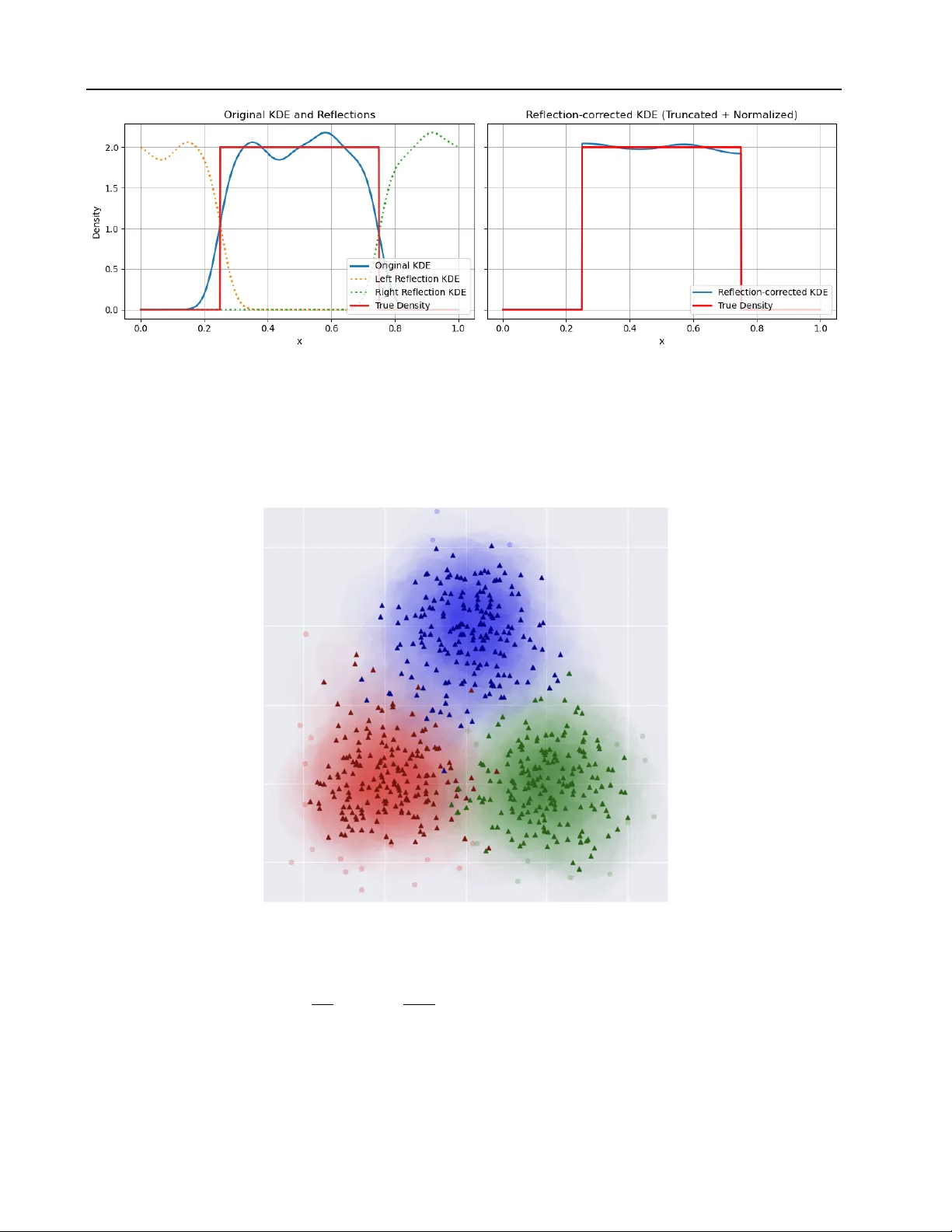
Symbolic Density Estimation: A Decompositional A ppr oach Angelo Rajendram 1 Xieting Chu 2 V ijay Ganesh 2 Max Fieg 3 Aishik Ghosh 2 Abstract W e introduce AI-K olmogorov , a novel frame work for Symbolic Density Estimation (SymDE). Sym- bolic regression (SR) has been effecti vely used to produce interpretable models in standard re gres- sion settings but its applicability to density esti- mation tasks has largely been une xplored. T o ad- dress the SymDE task we introduce a multi-stage pipeline: (i) problem decomposition through clus- tering and/or probabilistic graphical model struc- ture learning; (ii) nonparametric density estima- tion; (iii) support estimation; and ﬁnally (i v) SR on the density estimate. W e demonstrate the ef- ﬁcacy of AI-K olmogorov on synthetic mixture models, multivariate normal distributions, and three exotic distrib utions, two of which are moti- vated by applications in high-ener gy physics. W e show that AI-K olmogorov can disco ver underly- ing distrib utions or otherwise provide valuable insight into the mathematical expressions describ- ing them. 1. Introduction Data-driv en approaches are widely used to model complex nonlinear relationships between predicti ve features and tar - get variables. Popular approaches tend to be black-box and do not easily yield insight into underlying patterns in the data. Symbolic Regression (SR) is a family of methods that offer an interpretable alternati ve by searching the space of mathematical expressions and parameters to produce mod- els that re veal useful insights into the structure underlying the data. While SR has seen success in supervised learning tasks such as regression and dif ferential equation discovery , 1 Department of Mathematics, Univ ersity of W aterloo, W aterloo, Canada 2 Department of Computer Science, Georgia T ech, Atlanta, USA 3 Univ ersity of California, Irvine, Irvine, USA. Correspon- dence to: Angelo Rajendram < aa3rajen@uwaterloo.ca > , Xieting Chu < creatixchu@gatech.edu > , V ijay Ganesh < vganesh45@gatech.edu > , Max Fieg < mﬁeg@uci.edu > , Aishik Ghosh < AishikGhosh@physics.gatech.edu > . Preliminary work. Under re vie w by the International Conference on Machine Learning (ICML). Do not distribute. extending SR to the unsupervised task of density esti- mation introduces unique challenges and remains largely unexplored. Classical methods for density estimation typically fall into one of two categories; parametric density estimation as- sumes a model for the distribution and ﬁnds the best-ﬁtting parameters, and nonparametric density estimation av oids model assumptions but sacriﬁces interpretability . This work addresses the problem of Symbolic Density Estimation (SymDE) using symbolic regression to discov er mathemati- cal expressions that accurately describe continuous probabil- ity distributions. Searching the space of closed-form expres- sions a voids the restricti ve model assumptions of parametric density estimation while retaining interpretability unlike nonparametric density estimation. The SymDE problem faces three primary challenges: (i) ensuring v alidity constraints on probability distributions, namely non-negati vity and normalization o ver the support of the distribution; (ii) the curse of dimensionality; and (iii) the difﬁculty of disco vering comple x symbolic expressions from a vast search space. Related W ork SR is an established area of research with sev eral promising deep learning based approaches emerging ov er recent years. Howe v er , literature on the application of SR to discov er probability distrib utions from raw samples is scarce. Aside from seminal works on SR, few w orks that address the SymDE are mentioned here. Symbolic Re gr ession: SR is classically approached with genetic programming (GP) ( Koza , 1992 ), with PySR ( Cran- mer , 2023 ) currently among the state-of-the-art tools. These algorithms employ genetic operations (crossov er , mutation) to ev olve expressions ov er successiv e generations, ev alu- ating them using some measure of ﬁtness. The methods presented in this paper use PySR as the engine for SymDE, although another popular SR engine may also be used. Deep Learning-Based SR: Recent advances that apply deep learning methods to discov er descripti ve mathematical e x- pressions directly from data include Deep Symbolic Regres- sion (DSR) ( Petersen et al. , 2021 ) which uses reinforce- ment learning (RL). Neural-Guided Genetic Programming 1 Symbolic Density Estimation (NGGP) ( Mundhenk et al. , 2021 ) combines RL with GP . T ransformer-based techniques include NeSymReS ( Biggio et al. , 2021 ), SymbolicGPT ( V alipour et al. , 2021 ), and E2ESR ( Kamienny et al. , 2022 ). Finally , LASR ( Grayeli et al. , 2024 ) enhances GP by integrating learned concept libraries guided by LLMs, introducing a mechanism that brings the technique closer to the human scientiﬁc disco very process. Decomposition-Based Methods: Other methods lik e AI Feynman ( Udrescu & T egmark , 2020 ) and AI Feynman 2.0 ( Udrescu et al. , 2020 ), integrate neural networks with recur- siv e decomposition strate gies for equation discov ery , aiming to reduce the combinatorial explosion of the symbolic search space. Symbolic Regression using Control V ariables ( Jiang & Xue , 2023 ; Chu et al. , 2024 ) also attempts to address this issue by decomposing multi-variable SR into single-variable problems. These methods directly inspire our technique of decomposing high-dimensional distrib utions into simpler components. Symbolic Density Estimation: Maximum-Entropy based stochastic and symbolic density estimation (MESSY) ( T ohme et al. , 2024 ) is a symbolic density estimation frame- work that recovers analytical forms of probability density functions from sample data. It constructs a gradient-based drift–diffusion process that connects observed samples to a maximum entropy ansatz. MESSY uses symbolic regres- sion to e xplore candidate basis functions for the exponent in the maximum entropy model. This approach yields tractable symbolic descriptions of densities with lo w bias and a cost that is linear in the number of samples and quadratic in the number of basis functions. While the maximum entropy structure ensures valid probability densities and enables re- cov ery of multimodal distributions through reﬁnement, it does constrain the class of e xpressible densities compared with fully general functional forms. Morales-Alvarado 2025 apply the LLM-SR (Large Lan- guage Model for Symbolic Regression) framew ork from Shojaee et al. 2025 to benchmark problems of equation re- cov ery in lepton angular distributions and functional forms for angular coef ﬁcients in electroweak boson production. LLM-SR treats equations as programs with mathematical operators and combines LMMs’ scientiﬁc prior knowledge with ev olutionary search over equation programs. It itera- tiv ely proposed new equation skeleton hypotheses which are subsequently optimized against to ﬁnd the best parame- ters. While it takes advantage of a v ailable scientiﬁc domain knowledge, LLM-SR is limited to the av ailable training data which may lead to biases or gaps. Our Contributions W e introduce AI-K olmogorov , a framew ork for solving the SymDE problem and bridge the gap between nonparametric and parametric density estima- tion. While pre vious approaches address partial aspects of this problem, the y do not search o ver truly general symbolic functional forms for distributions in higher dimensional settings. Symbolic regression tools cannot directly solve SymDE because the training dataset typically does not con- tain density labels. W e explore ev olutionary algorithms such as in PySR ( Cranmer , 2023 ) which could use log-likelihood scores b ut ﬁnd that the resultant expressions may not ad- here to the non-negati vity and normalization constraints that ev ery v alid distribution must satisfy . W e conduct experiments that demonstrate the efﬁcac y of AI-K olmogorov and sho wcase its results on v arious datasets. Our ev aluation includes synthetic datasets such as multi- variate normal distributions and mixture models, and other problems using non-standard distributions. W e present abla- tions studies that e v aluate the utility of the decomposition techniques proposed. The results show that AI-K olmogorov provides useful information about the structure of the under- lying distributions, producing interpretable symbolic mod- els with low residual error and effecti v ely trading off model complexity and accuracy , demonstrating the framework’ s ability to aid the discovery of interpretable mathematical expressions that describe probability distrib utions. 1 2. Background Symbolic Regression Giv en a dataset D = { ( x i , y i ) } N i =1 , the goal is to identify a function f such that the target v ari- able y i ≈ f ( x i ) ∀ i ∈ { 1 , 2 , .., N } . SR discovers mathe- matical expressions that predict the tar get from the feature variables while balancing model accurac y and complexity . The ideal models are accurate yet parsimonious. Unlike traditional regression that ﬁts parameters for a ﬁxed model class, SR instead e xplores a v ast space of potential mathe- matical expressions to ﬁnd the most suitable representation. The search space of e xpressions grows e xponentially with the number of permitted operators and variables. Candidate models are constructed as e xpression trees from operators and v ariables, adhering to a context-free grammar . SR has been sho wn to be NP-hard ( V irgolin & Pissis , 2022 ), but de- spite the computational challenges, SR offers the possibility of interpretability which is central to scientiﬁc discov ery . Probability Distrib utions and Density Estimation A probability distribution assigns probabilities to outcomes of a random variable. For continuous variables, the probability density function (PDF) f X ( x ) satisﬁes f X ( x ) ≥ 0 (non- negati vity constraint) and R f X ( x ) d x = 1 (normalization constraint). Density estimation approximates the probability distribu- 1 https://anonymous.4open.science/r/SymbolicDensityEstimation- 31D4 2 Symbolic Density Estimation tion from samples. Given i.i.d. samples X 1 , X 2 , ..., X n from unknown distrib ution f X ( x ) , the goal is ﬁnd an esti- mate ˆ f X ( x ) . K ernel Density Estimation (KDE) is a widely used calssic nonparametric technique where each data point contributes a localized k ernel function, ˆ f n ( x ) = 1 nh d n X i =1 K  x − X i h  , where h is the bandwidth (a smoothing hyper -parameter) and K is the kernel function. While adequate for simple distributions, it’ s performance suffers in higher dimensions or for distributions that hav e sharp discontinuities at the boundaries of the support. Normalizing Flo ws (NFs) hav e recently emerged as a po w- erful alternati ve for nonparametric density estimation, par - ticularly in high-dimensional spaces. Unlike KDE, which constructs a density by summing local k ernels, NFs learns an expressi ve density by transforming a simple base distri- bution f Z ( z ) (e.g., a standard multiv ariate Gaussian) into a complex tar get distribution via a sequence of in vertible, dif- ferentiable mappings x = g ( z ) . By parameterizing g with deep neural netw orks that ensure tractability of the Jacobian determinant, NFs can model highly intricate distributions while allowing for e xact likelihood e valuation and ef ﬁcient sampling. In Symbolic Density Estimation (SymDE), the challenge is not only to e valuate the density function at any given query points, b ut to obtain a symbolic description of the distribution. SymDE goes beyond the f amiliar families of distributions used in parametric density estimation and the black-box nature of nonparametric density estimation to discov er descripti ve mathematical expressions for exotic distributions. 3. Method 3.1. The AI-Kolmogor ov framew ork The frame work is illustrated in Figure 1 . T o disco ver the un- derlying continuous probability density function, we employ optional preprocessing stages to decompose the problem. Then non-parameteric density estimation produces a black- box model of the distribution that can be ev aluated at any query point to provide a density estimate. This is followed by symbolic re gression to obtain candidate symbolic expres- sions for the underlying probability density function. The nonparametric density estimate acts as a surrogate target for symbolic regression imposing non-negativity and normal- ization as soft constraints via the mean squared error (MSE) loss computed ov er a re gular grid of e valuation points in the distribution’ s support. Clustering Clustering is useful for multi-modal data where the modes are well separated. The raw samples are segmented into unimodal clusters before calling symbolic regression on each distinct cluster . Once expressions for each cluster are identiﬁed, they can be combined additiv ely . The model complexity for each cluster individually may be simpler than that for the full distrib ution, improving the odds of SR ﬁnding simpler expressions that can be com- bined afterwards. An example of an algorithm that can be used for this decomposition is DBSCAN ( W ang et al. , 2019 ), a density-based clustering method that automatically infers the number of clusters without parametric assumptions on the shape of the clusters. Structure Lear ning If clustering enables additiv e decom- position,then structure learning enables multiplicati ve de- composition. Structure learning entails identifying the de- pendence or independence between covariates or equiv- alently , determining the underlying Probabilistic Graph- ical Model (PGM). If independent subsets of cov ariates are detected the computational cost of SymDE on high- dimensional distributions can be dramatically reduced. Each independent subset of co variates appear as a separate con- nected component in the PGM. SR can be performed on the subset of cov ariates within each connected component separately , reducing the dimensionality of the problem to be tackled. For example, in the case of a 4-dimensional distribution where two pairs of co variates are independent, the joint distrib ution can be factorized as a product of tw o 2-dimensional distributions. W e use the constrained-based learning PC algorithm ( Neapolitan , 2003 ) (refer to Appendix B ) for structure-learning in continuous data. This makes use of statistical tests to construct probabilistic graphical mod- els and identify the connected components to signiﬁcantly reduce computational cost for SR. Nonparametric Density Estimation Nonparametric Den- sity Estimation serves as the bridge between raw data and symbolic regression, producing a black-box model of the un- known distribution. W ith K ernel Density Estimation (KDE), each data point contrib utes a localized “bump” and the o ver - all estimate is obtained by summing these contributions ov er the support. W e employ Gaussian kernels and select the bandwidth using cross-validation. In cases where KDE provides inadequate density estimates we use Neural Spline Flows (NSF) ( Durkan et al. , 2019 ), a powerful class of normalizing ﬂo ws. While simpler NFs of- ten rely on afﬁne mappings, NSF utilizes monotonic rational- quadratic splines to transform a simple base distrib ution into a complex target distribution. By using a neural network to parameterize the locations and deriv ativ es of the spline knots, the model can capture intricate, multi-modal features that simpler ﬂows miss. This combination of high expres- 3 Symbolic Density Estimation F igur e 1. The AI-K olmogorov pipeline: decomposition (clustering/structure learning), density estimation, support estimation, symbolic regression, and warm-start reﬁnement. Optional workﬂo ws are indicated by dashed arrows. sivity and numerical stability makes NSF a state-of-the-art choice for modeling high-dimensional data where traditional non-parametric methods like KDE may struggle with the curse of dimensionality . Support Estimation Support estimation identiﬁes the sub- set of the input space X ⊆ R d where the density func- tion f X ( x ) is strictly positiv e, prev enting the algorithm from searching for expressions that attempt to ﬁt discon- tinuites at the boundaries of a distribution. W e employ lev el-set thresholding on the non-parametric density esti- mate: b S τ = { x ∈ R d | ˆ f n ( x ) ≥ τ } where τ > 0 is a small threshold. Alternativ ely for distributions with con v ex supports, the con vex hull of the samples may be used to esti- mate the support. T o correct any bias of the non-parametric density estimates at boundaries with sharp discontinuities, we employ the reﬂection trick if the boundaries are straight lines or otherwise apply a shrinking factor to the estimated support to a void trim re gions near the boundary where we know the density estimate is inaccurate. Refer to Appendix B.1 for more details. Symbolic Regression The density estimate from the non- parametric model is used as the target v ariable in SR. The MSE loss with respect to the density estimate serves as a sur- rogate loss function for density estimation. W e make use of PySR as the computational engine for Symbolic Regression, which employs multi-population e volutionary algorithms to search the space of mathematical expressions. Each can- didate expression is e valuated using a ﬁtness function that balances the MSE loss against model comple xity as mea- sured by the size of the expression tree. This multi-objecti v e optimization approach fa vors the discov ery of expressions that are both accurate and parsimonious. The set of oper - ators for each problem may be selected based on expert knowledge. For all e xamples provided in this work, the set of permitted operators is a superset of the operators that ap- pear in the ground truth expression (except for the results in Section 4.4 ). The output of SR is pareto front of expressions trading off accuracy against complexity allowing users to examine a zoo of models. Simpler models capture coarse structure and more comple x models are able to capture e ven ﬁne grained variation in the data. 4. Results W e ev aluate AI-K olmogoro v to demonstrate its merits and weaknesses on various datasets. For all datasets, we assume sample sizes are sufﬁciently lar ge. 4.1. Additive and Multiplicati ve Decomposition Clustering and structure learning pro vide two complemen- tary strategies for decomposing comple x distributions into simpler sub-problems. Clustering assumes an additiv e fac- torization and reduces the complexity of the symbolic ex- pressions to be discov ered per component, while structure learning assumes multiplicative factorization and reduces both target expression complexity and the dimensionality per component. T o demonstrate clustering, we consider X ∈ R 2 drawn from a two-component Gaussian mixture: f X ( x ) = 1 2 N ( x | µ 1 , Σ ) + 1 2 N ( x | µ 2 , Σ ) , with µ 1 =  − 4 . 0 4 . 0  , µ 2 =  4 . 0 − 4 . 0  , Σ =  1 0 . 8 0 . 8 1  . This distribution can be decomposed the sum of two Gaus- sian components. W e denote x = ( x 1 , x 2 ) T . 4 Symbolic Density Estimation (a) Additive decompositon: Results on the Gaussian mixture dataset. Prediction (left) and residuals (center left) by AI-Kolmogoro v . Prediction (center right) and residuals (right) by clustering augmented AI-K olmogorov . (b) Multiplicativ e decomposition: Results on the the 4-dimensional Gaussian dataset. Prediction (left) and residuals (center left) by AI-K olmogorov . Prediction (center right) and residuals (right) by structure learning augmented AI-Kolmogoro v . Only the marginal N ( x 2 | µ 2 , Σ ) is shown. F igur e 2. Ablation study on clustering and structure learning. T op: clustering results. Bottom: structure learning results. Figure 2a is an ablation study of AI-K olmogorov with and without augmentation by clustering. The left two panels show the prediction and residuals of the most accurate e x- pression reco vered by AI-K olmogorov ; the right two panels show the prediction and residuals of clustering augmented AI-K olmogorov . The maximimum predicted density and absolute residual are 0.129 and 0.005 respectiv ely (left two panels in Figure 2a ), and 0.129 and 0.004 respectiv ely (right two panels Figure 2a ). The residuals of both approaches are similar in magnitude (T able 1 ), but the factored models yield more interpretable symbolic forms since the addition of the two component distrib utions is explicitly captured and the true symbolic expressions per component are simpler . The pareto fronts and recov ered expressions for the Gaussian mixture dataset can be found in Appendix C.1 . W e next demonstrate structure learning using independent random vectors X 1 , X 2 ∈ R 2 , concatenated as X ∈ R 4 . The joint distribution is f X ( x ) = N ( x 1 | µ 1 , Σ ) · N ( x 2 | µ 2 , Σ ) , which deﬁnes a 4D distribution whose PGM has two con- nected components corresponding to N ( x 1 | µ 1 , Σ ) and N ( x 2 | µ 2 , Σ ) . W e denote x 1 = ( x 1 , x 2 ) T and x 2 = ( x 3 , x 4 ) T . The parameters for each component were set identically to those in the previous e xample. Figure 2b is an ablation of AI-Kolmogoro v against AI- K olmogorov augmented with structure learning. T o vi- sualize the result, we only show the results for mar ginal N ( x 2 | µ 2 , Σ ) . F or the panels corresponding to direct ap- plication of the pipeline to the 4D Gaussian distrib ution, the 2D marginal w as computed by numerically integrating out the remaining variables. Decomposition yields signiﬁcantly lower error (see T able 1 ) for the most complex models on the pareto front. The maximimum predicted density and absolute residual are 0.630 and 0.506 respectiv ely (left two panels of Figure 2b ), and 0.258 and 0.002 respectively (right two panels of Figure 2b ). For an y giv en error lev el the sym- bolic expressions for each component are more compact and easier to interpret. While the distributions are not recov ered exactly , the recov ered expressions are still suggestive as they in volve e xponentials with negati ve sum of squares in the exponent. The pareto fronts and recovered e xpressions for the 4D Gaussian dataset can be found in Appendix C.2 . T able 1. MSE comparison between direct application of AI- K olmogorov and augmented AI-K olmogorov . The MSE with decomposition reﬂects the MSE after recombining the most accu- rate expressions from the pareto fronts Dataset MSE without decomposition MSE with decomposition Gaussian mixture 4 . 71 × 10 − 4 3 . 57 × 10 − 4 4D Gaussian 1 . 01 × 10 − 3 4 . 24 × 10 − 5 5 Symbolic Density Estimation 4.2. Rastrigin Synthetic Dataset W e use a Rastrigin function as a synthetic exotic probability density function to demonstrate the strengths of the pipeline. The Rastrigin function is a non-con vex function commonly used to benchmark optimization algorithms, but it is not typically encountered as a probability distribution. T o adapt it into a valid distribution, we constrain its sup- port, normalize it, and apply a bias to ensure non-negativity . Samples are drawn from this distrib ution using rejection sampling ov er the range x 1 , x 2 ∈ [ − 2 , 2] , f ( x ) = 1 586 . 67 h 10 + 2 X i =1 10 x 2 i − 5 cos(3 π x i − 6 . 1) i Figure 3 illustrates the AI-K olmogoro v prediction and the residual error between the most accurate e xpression recov- ered and the ground truth. The residual plot shows that the symbolic expression reco vered by AI-K olmogoro v closely matches the true density surface. F igur e 3. Prediction (left) and residuals with respect to the ground truth (right) of the lo west loss expression. The maximum predicted density and absolute residual are 0.140 and 0.003 respectiv ely . Expressions on the simpler end of the pareto front such as 1 . 5 + x 2 1 + x 2 2 which captures the ”coarse” bowl shape, and we recov er what resembles the true expression on the more complex end of the pareto front (see Appendix C.3 ) 1 . 1( x 2 1 + x 2 2 ) − 0 . 56(cos(9 . 4 − 12) − 0 cos(9 . 4 x 2 + 13)) + 1 . 1 4.3. Muon Decay The next example is motiv ated by applications in particle physics. The dataset describes muon decay , where a muon decays into an electron, and electron-antineutrino and a muon-neutrino. The features m 2 13 and m 2 23 are combinations of the momenta and energies of the outgoing particles. More speciﬁcally , the in v ariant mass of two-particle system where 1,2,3 labels the electron-antineutrino, the electron, and the muon-neutrino respecti vely . The ground-truth density ( i.e. the dif ferential decay width with respect to m 13 , m 23 ) takes the form N × ( m 2 23 − m 2 µ )( m 2 23 − m 2 e ) ( m 2 13 + m 2 23 − m 2 e − m 2 µ + m 2 W ) 2 a rational function with a quadratic numerator in m 2 23 and a quadratic denominator in both m 2 13 and m 2 23 with normaliza- tion constant N . W e simulate samples of these e vents with the Monte-Carlo ev ent generator Madgraph ( Alwall et al. , 2014 ); ho wev er , note that we have performed the simulation such that the masses of the electron ( m e ) and muon ( m µ ) are comparable to the mass of the W -boson ( m W ) so that there is a non-tri vial dependence on m 13 in the density (in nature, m W ≫ m e , m µ ). Otherwise, the problem would be ef fectiv ely 1-dimensional. This distrib ution could arise if there were an e xotic W ′ -boson with a mass comparable to the masses of distinct fermion generations. The masses used for m µ , m e , and m W are 78 GeV , 70 GeV , and 80.4 GeV respectiv ely . W e apply min–max scaling to normalize the range of both features. This preserves the functional form of the distribu- tion up to an afﬁne transformation on each feature. Figure 4 shows the prediction and the residual error between the recov ered symbolic density and the KDE. A con ve x hull trimming procedure (Appendix B.1 ) was used to estimate the support. No samples lie outside this region as it would violate energy/momentum conservation, but the support is estimated here without this domain knowledge. F igur e 4. Prediction and regions for local probability mass vali- dation indicated as A & B (left). Residuals with respect to KDE (right) of the lowest loss expression. The maximum predicted density is 3.677, and the maximum absolute residual is 0.640. Muon decay local probability mass validation T o av oid relying on the availability of a ground truth expression to validate the KDE and symbolic density estimate (the most accurate expression recovered) we instead examine the prob- ability mass ov er two small square re gions (Figure 4 ). The empirical probability mass o ver each square region is ob- tained by ﬁnding the fraction of raw samples that are present inside each square. W e then integrate both the KDE and 6 Symbolic Density Estimation T able 2. Muon decay local probability mass validation on two 0 . 02 × 0 . 02 square regions. Method Region A Region B Empirical 1 . 4960 × 10 − 3 9 . 3200 × 10 − 4 KDE 1 . 4811 × 10 − 3 9 . 1705 × 10 − 4 SR 1 . 4638 × 10 − 3 9 . 1224 × 10 − 4 symbolic density estimate numerically over these regions to compute an estimated probability mass. Finally , we compare the estimated probability mass from the density estimates to the empirical probability mass to assess if they ﬁt the true distribution well. The results in T able 2 suggest that the density estimates are accurate in the two regions examined. The pareto front of re- cov ered expressions is reported in Appendix C.4 . Although the exact form is not recov ered, the resulting e xpressions achiev e very low error with respect to the KDE within the support of the distribution. 4.4. Dijet T o test our frame work on a more challenging dataset, we simulate the production of two jets in proton-proton colli- sions at the Large Hadron Collider . This process depends in part on the content of the proton, the “parton distribution function” (we use NNPDF2.3 ( Ball et al. , 2013 )) as well as the model of hadronization. The parton distribution cannot be calculated from ﬁrst principles and must instead be de- riv ed from experiment with an assumed model. A v ariety of models are assumed ( Dulat et al. , 2016 ; Ball et al. , 2015 ), and thus can represent a bias that must be considered ( Gao & Nadolsky , 2014 ); a similar statement could be said of the hadronization model, but we perform our analysis at parton- lev el. One could thus imagine using our symbolic regression to either gain insight into the underlying truth distribution, or point tow ards more promising and less-considered func- tional forms. There are man y observ ables that one could use to gain insight, we choose two high-lev el observables which are calculated from the simulation: the in v ariant mass of the jet pair , m j j , and the scalar sum of the transverse momenta, H T = P 1 , 2 | p i T | . Note that these observables are chosen some what arbitrarily and are not optimized for the problem at hand. Our goal is to test our framew ork on a problem where the understanding of underlying distribution is on less solid footing. F igur e 5. Prediction and regions for local probability mass vali- dation indicated as A & B (left). Residuals with respect to NSF (right) of the lowest loss expression. The maximum predicted density is 4555.25 and the maximum absolute residual is 1789.14. This dataset set is particularly challenging because of the presence of sharp discontinuities at the boundary of the sup- port and because the distribution is concentrated in a small region. Figure 5 shows the prediction and the residual error between the recov ered symbolic density and the NSF den- sity estimate. The residuals reported are lar ge, though this may be attrib uted to the sharp discontinuity near the distri- bution peak. The heat map of the prediction is qualitativ ely similar to the distribution of ra w samples. Dijet local probability mass v alidation Similarly to the previous e xample of Muon Decay , we examine the proba- bility mass over two small square regions (Figure 5 ). The results in T able 3 suggest that the density estimate obtained by NSF outperforms KDE. This can also be seen in the log- likelihood scores in Figure 6 .The SR stage uses the NSF density estimate, as the accuracy of KDE w ould otherwise hav e been a bottleneck to the method. T able 3. Dijet local probability mass validation on two 0 . 02 × 0 . 02 square regions. Method Region A Region B Empirical 1 . 0270 × 10 − 1 2 . 3200 × 10 − 3 KDE 6 . 7234 × 10 − 2 1 . 5040 × 10 − 2 NSF 1 . 0974 × 10 − 1 1 . 9397 × 10 − 3 SR 1 . 1493 × 10 − 1 2 . 2609 × 10 − 3 7 Symbolic Density Estimation F igur e 6. Mean log-likelihood scores against expression complex- ity for SR using only MSE loss and SR using MSE, mean negati ve log-likelihood (NLL), and penalties for negati ve density predic- tions (NP) in the loss function. Triangles indicate e xpressions that made negati ve predictions on test samples. Figure 6 shows the mean log-likelihood scores of the ex- pressions discovered by AI-K olmogorov using only MSE loss versus a combination of MSE loss, mean ne gati ve log- likelihood, and penalties for ne gati ve predictions. The vol- ume under each expression was normalized prior to com- puting their mean log-likelihood scores. The results suggest that loss function design may improve both accuracy and validity of the returned expressions. Accurate models may be discov ered using MSE loss only , though these are more likely to return negativ e predictions over the test samples (indicated by triangles on the markers in Figure 6 ). Although the log-likelihood scores appear to drop off for expressions with complexity greater than 10 in Figure 6 for SR MSE this was due to some of them producing small negati ve predictions on a small subset of the test set (at most 282 out of 10,000 test samples). The density predictions are clipped if they fall below a tiny threshold, and their log-likelihood scores are sensitiv e to the selected clipping threshold. Tuning the constants of the recov ered expressions with an additional bias term could be done to satisfy the non-negati vity constraint and potentially improv e the log- likelihood score. Augmenting the loss function with the negati ve log-likelihood (SR MSE + NLL + NP) does not appear to have a signiﬁcant impact on the performance of SR nor does it perform as well as SR with only the MSE and negati ve prediction penalties (SR MSE + NP) with respect to the log-likelihood metric on this particular problem. Nevertheless, it injects context of the original density estimation problem into AI-K olmogorov’ s SR stage, and may still be useful on other problems with appropriately tuned weights. SR MSE + NP appears to have a slight improv ement ov er the NSF , howe ver , these expressions do not strictly satisfy the constraints of a valid distribution, while NSF does by construction. These expressions may nev ertheless hav e terms useful for interpretability . Finally , an attempt was made using SR without MSE and only the negati ve log-likelihood loss and the negati ve pre- diction penalty . This loss function produced expressions that did not ﬁt the distrib ution well, achieving a maximum mean log-likelihood score of -0.12, consequently it does not appear on the scale in Figure 6 The pareto front of recovered expressions is reported in Appendix C.5 . The loss function only softly enforces nor- malization via MSE loss against the NSF density estimate ov er a regular grid in the support. 4.5. Key Insights and Obser vations Clustering (additive decomposition): Identiﬁes well- separated modes and ﬁts unimodal components before re- combination by summation; interpretability improv es with- out sacriﬁcing accuracy . Structure lear ning (multiplicative decomposition): Ex- ploits independence between subsets of the covariates to reduce dimensionality at the SR stage; this yields markedly lower errors and more compact expressions than non- decomposed baselines. Support Estimation: Improv es stability and interpretabil- ity; meaningful symbolic descriptions may only be v alid ov er the support without sharp discontinuities in the tar get probability density function. Nonparametric density estimate: Poor nonparamet- ric density estimates bottleneck the performance of AI- K olmogorov’ s SR stage. Loss function design: MSE against the nonparametric density estimate over a regular grid is typically sufﬁcient to obtain accurate models although additional loss function design has beneﬁts. Raw samples and log-likelihood alone may result in in v alid models as expressions that predict negati ve densities or lar ge density in regions where samples are sparse are not penalized. With GP-based SR, the loss function need not be differentiable, ho wev er , other methods may require this property . Exploration of symbolic expr essions: W ith limited do- main speciﬁc context, a di versity of candidate models may inform scientists of interesting structure present in the ra w samples. 8 Symbolic Density Estimation 5. Future W ork and Conclusion There are sev eral possible extensions to AI-Kolmogoro v for SymDE that warrant further in vestigation. The current ap- proach provides a solid foundation by demonstrating the fea- sibility of combining decomposition strategies with state-of- the-art symbolic regression techniques. Future work could explore more sophisticated decomposition strate gies.The incorporation of the likelihood, computed on the ra w input samples, directly into the loss has shown promise. W ith sufﬁcient complexity , it outperforms the neural density es- timator . Howe ver , labels from the neural density estimator helps stabilize the search algorithm. Future work could in- corporate the normalization requirement of densities though a Monte-Carlo integration into the loss. Agentic AI frame- works for SymDE are also a promising av enue for future work. Equally important is the dev elopment of principled diag- nostics to assess goodness-of-ﬁt, especially for heavy-tailed distributions and small-sample settings. Real-world distri- butions may ha ve heavy tails and understanding the per - formance and understanding the limitations of our tool in small sample regime would be necessary . Applying AI- K olmogorov to real-w orld problems in physics, ﬁnance, and other domains would pro vide valuable insights with practi- cal utility , and help the development of domain-speciﬁc and interpretable statistical models. Impact Statement This paper presents a work whose goal is to advance the ﬁeld of Machine Learning. There are many potential societal consequences of our work, none which we feel must be speciﬁcally highlighted here. References Alwall, J., Frederix, R., Frixione, S., Hirschi, V ., Maltoni, F ., Mattelaer , O., Shao, H. S., Stelzer , T ., T orrielli, P ., and Zaro, M. The automated computation of tree-level and next-to-leading order dif ferential cross sections, and their matching to parton shower simulations. JHEP , 07:079, 2014. doi: 10.1007/JHEP07(2014)079. Ball, R. D., Bertone, V ., Carrazza, S., Del Debbio, L., Forte, S., Guffanti, A., Hartland, N. P ., and Rojo, J. Parton distributions with QED corrections. Nucl. Phys. B , 877: 290–320, 2013. doi: 10.1016/j.nuclphysb .2013.10.010. Ball, R. D. et al. Parton distributions for the LHC Run II. JHEP , 04:040, 2015. doi: 10.1007/JHEP04(2015)040. Biggio, L., Bendinelli, T ., Neitz, A., Lucchi, A., and Paras- candolo, G. Neural symbolic regression that scales. In International Confer ence on Machine Learning , pp. 936– 945. Pmlr , 2021. Bishop, C. M. and Bishop, H. Deep Learning - F ounda- tions and Concepts . Springer , Cham, 1 edition, 2023. ISBN 978-3-031-45468-4. doi: https://doi.org/10.1007/ 978- 3- 031- 45468- 4. Chen, Y .-C. A tutorial on kernel density estimation and recent advances. Biostatistics & Epidemiology , 1(1):161– 187, 2017. Chu, X., Zhao, H., Xu, E., Qi, H., Chen, M., and Shao, H. Scalable neural symbolic re gression using control variables, 2024. URL 2306.04718 . Cranmer , M. Interpretable machine learning for science with pysr and symbolicregression. jl. arXiv preprint arXiv:2305.01582 , 2023. Cui, L. Shape and Geometry in Statistics: Support and Density Estimation . Ph.d. dissertation, University of California, Davis, Da vis, CA, 2021. URL https:// escholarship.org/uc/item/9v21t0zw . Pro- Quest ID: Cui ucda vis 0029D 20897; Merritt ID: ark:/13030/m5b34thp. Dulat, S., Hou, T .-J., Gao, J., Guzzi, M., Huston, J., Nadol- sky , P ., Pumplin, J., Schmidt, C., Stump, D., and Y uan, C. P . Ne w parton distrib ution functions from a global analysis of quantum chromodynamics. Phys. Rev . D , 93 (3):033006, 2016. doi: 10.1103/PhysRe vD.93.033006. Durkan, C., Bekasov , A., Murray , I., and Papamakarios, G. Neural spline ﬂo ws, 2019. URL https://arxiv. org/abs/1906.04032 . Gao, J. and Nadolsky , P . A meta-analysis of parton distri- bution functions. JHEP , 07:035, 2014. doi: 10.1007/ JHEP07(2014)035. Grayeli, A., Sehgal, A., Costilla-Reyes, O., Cranmer , M., and Chaudhuri, S. Symbolic regression with a learned concept library , 2024. URL abs/2409.09359 . Jang, J. and Jiang, H. Dbscan++: T owards fast and scal- able density clustering, 2019. URL https://arxiv. org/abs/1810.13105 . Jiang, N. and Xue, Y . Symbolic regression via control variable genetic programming, 2023. URL https:// arxiv.org/abs/2306.08057 . Kamienny , P .-A., d’Ascoli, S., Lample, G., and Charton, F . End-to-end symbolic regression with transformers. Advances in Neural Information Pr ocessing Systems , 35: 10269–10281, 2022. 9 Symbolic Density Estimation K oza, J. R. Genetic pr ogramming: on the pr ogramming of computers by means of natural selection . MIT Press, Cambridge, MA, USA, 1992. ISBN 0262111705. Morales-Alvarado, M. Foundation models for equation discov ery in high ener gy physics, 2025. URL https: //arxiv.org/abs/2510.03397 . Mundhenk, T . N., Landajuela, M., Glatt, R., Santiago, C. P ., Faissol, D. M., and Petersen, B. K. Symbolic regres- sion via neural-guided genetic programming population seeding. arXiv pr eprint arXiv:2111.00053 , 2021. Neapolitan, R. E. Learning Bayesian Networks . Prentice- Hall, Inc., USA, 2003. ISBN 0130125342. Petersen, B. K., Landajuela, M., Mundhenk, T . N., Santi- ago, C. P ., Kim, S. K., and Kim, J. T . Deep symbolic regression: Recov ering mathematical expressions from data via risk-seeking policy gradients. In Proc. of the International Confer ence on Learning Repr esentations , 2021. Shojaee, P ., Meidani, K., Gupta, S., Farimani, A. B., and Reddy , C. K. Llm-sr: Scientiﬁc equation discovery via programming with large language models, 2025. URL https://arxiv.org/abs/2404.18400 . T ohme, T ., Sadr, M., Y oucef-T oumi, K., and Hadjiconstanti- nou, N. G. Messy estimation: Maximum-entropy based stochastic and symbolic density estimation, 2024. URL https://arxiv.org/abs/2306.04120 . Udrescu, S.-M. and T egmark, M. Ai feynman: A physics- inspired method for symbolic re gression. Science Ad- vances , 6(16):eaay2631, 2020. Udrescu, S.-M., T an, A., Feng, J., Neto, O., W u, T ., and T egmark, M. Ai fe ynman 2.0: P areto-optimal symbolic regression exploiting graph modularity . In Larochelle, H., Ranzato, M., Hadsell, R., Balcan, M., and Lin, H. (eds.), Advances in Neural Information Pr ocessing Systems , volume 33, pp. 4860–4871. Curran Associates, Inc., 2020. URL https://proceedings.neurips. cc/paper_files/paper/2020/file/ 33a854e247155d590883b93bca53848a- Paper. pdf . V alipour , M., Y ou, B., Panju, M., and Ghodsi, A. Sym- bolicgpt: A generativ e transformer model for symbolic regression. arXiv preprint , 2021. V irgolin, M. and Pissis, S. P . Symbolic regres- sion is np-hard. T r ans. Mach. Learn. Res. , 2022, 2022. URL https://api.semanticscholar. org/CorpusID:250264685 . W ang, D., Lu, X., and Rinaldo, A. Dbscan: Optimal rates for density based clustering, 2019. URL https:// arxiv.org/abs/1706.03113 . 10 Symbolic Density Estimation A. A ppendix: Mathematical Foundations A.1. Probabilistic Graphical Models Any probability distribution can be represented as a directed acyclic graph (D A G) where nodes represent ran- dom variables and links represent probabilistic relationships. The joint distribution factorizes as p ( x 1 , ..., x n ) = p ( x n | x 1 , ..., x n − 1 ) ...p ( x 2 | x 1 ) p ( x 1 ) . F igur e 7. Example PGM for distribution p ( x 1 , ..., x 7 ) = p ( x 1 ) p ( x 2 ) p ( x 3 ) p ( x 4 | x 1 , x 2 , x 3 ) · p ( x 5 | x 1 , x 3 ) p ( x 6 | x 4 ) p ( x 7 | x 4 , x 5 ) ( Bishop & Bishop , 2023 ). B. A ppendix: Algorithmic Details B.1. Support Estimation The support of a probability distrib ution is supp( f X ) = { x ∈ R d | f X ( x ) > 0 } . Con v ex hull estimates impro ve boundary handling for bounded distributions. F igur e 8. Con vex hull support estimates. Left: true support. Right: con vex hull estimate ( Cui , 2021 ). T o correct bias of non-parametric density estimates at known boundaries of a distrib ution we can employ the reﬂection trick as illustrated in Figure 9 . 11 Symbolic Density Estimation F igur e 9. Reﬂection trick in one dimension. B.2. Clustering and Structure Lear ning DBSCAN clustering automatically infers cluster count and handles non-parametric cluster shapes. Structure learning discov ers independent variable subsets, enabling problem decomposition via the product rule. F igur e 10. DBSCAN on a 2D Gaussian mixture. Core points hav e ϵ -neighborhoods with at least minPts samples ( Jang & Jiang , 2019 ). B.3. Ker nel Density Estimation KDE estimates density as ˆ f n ( x ) = 1 nh d P n i =1 K  x − X i h  where h is bandwidth and K is kernel function. The reﬂection trick improv es boundary estimates by reﬂecting samples across boundaries. B . 3 . 1 . F A S T F O U R I E R T R A N S F O R M K D E Fast Fourier Transform (FFT) KDE is a computationally ef ﬁcient approach that leverages the con v olution theorem to accelerate density estimation. Instead of directly computing the sum of kernel functions at each ev aluation point, FFT KDE 12 Symbolic Density Estimation discretizes the domain into a regular grid and performs the con volution in the frequency domain. This approach transforms the computational comple xity from O ( nm ) to O ( n log n + m log m ) , where n is the number of samples and m is the number of grid points, making it particularly adv antageous for large datasets and ﬁne-grained density estimates. The method works by: (1) creating a histogram of the data on a regular grid, (2) computing the FFT of both the histogram and the kernel, (3) multiplying them in the frequenc y domain, and (4) applying the in v erse FFT to obtain the ﬁnal density estimate. This technique is especially effecti v e for multiv ariate data and is widely used in modern statistical software packages. F igur e 11. Kernel Density Estimation in 1D ( Chen , 2017 ) C. A ppendix: Experimental Results C.1. Gaussian Mixture Dataset T able 4. Hyper-parameters for symbolic re gression on the Gaussian mixture dataset Hyper -parameter V alue Notes Ker nel Density Estimation number of samples 450000 bandwidth 0.101 KDE bandwidth selected using cross-validation. PySR binary operators [+, -, *, /] unary operators [exp, log, po w2, pow3] Allowed unary operators. maxsize 50 Maximum size of an expression tree. ncycles per iteration 380 Cycles per iteration of the genetic algorithm. parsimony 0.001 Penalty for complexity of e xpressions. adaptiv e parsimony scaling 1040 Scales the penalty based on frequency of each com- plexity le vel niterations for SR 8000 Iterations for SR. num populations for SR 15 Number of populations for SR. population size for SR 30 Number of expressions per population in SR elementwise loss MSE Loss function used for SR. batch size 128 batch size of the dataset used to evaluate loss of expressions 13 Symbolic Density Estimation F igur e 12. Pareto front of recov ered expressions for the Gaussian mixture dataset. 14 Symbolic Density Estimation T able 5. Expressions simpliﬁed with sympy alongside their raw complexity score from PySR for the Gaussian mixture dataset. Raw Complexity Simpliﬁed Expression 1 0 . 13 2 0 . 14 3 0 . 13 5 0 . 14 6 0 . 24 − 0 . 0023 x 2 2 7 e − 0 . 23( x 1 + x 2 ) 2 9 2 e − 220  0 . 067 x 2 + 1 x 1  2 11 2 . 5 e − 16(0 . 062 x 1 x 2 +1) 2 13 3 . 1 e − 220( x 1 + x 2 ) 2 (0 . 067 x 1 x 2 +1) 2 x 2 1 14 13 e − ( x 1 + x 2 ) 2 − 260  0 . 062 x 2 + 1 x 1  2 15 e − x 2 2 − 290(0 . 059 x 1 x 2 +1) 2 +46 x 2 1 16 9 . 5 e − 0 . 15( x 1 + x 2 ) 2 − 220  0 . 067 x 2 + 1 x 1  2 18 9 . 9 e − 0 . 15( x 1 + x 2 ) 2 − 18(0 . 064 x 1 x 2 +1) 2 20 9 . 9 e − 0 . 15( x 1 + x 2 ) 2 − 18(0 . 064 x 1 x 2 +1) 2 + 0 . 0052 21 9 . 9 e − 0 . 15( x 1 + x 2 ) 2 − 19(0 . 062 x 1 x 2 +1) 2 + 0 . 0038 22 9 . 9 e − 0 . 15( x 1 + x 2 ) 2 − 19(0 . 062 x 1 x 2 +1) 2 + 0 . 0041 23 9 . 9 e − 18(0 . 064 x 1 x 2 +1) 2 − 0 . 29 0 . 71 x 1 +0 . 71 x 2 + 1 x 3 1 ! 2 24 9 . 9 e − 19(0 . 062 x 1 x 2 +1) 2 − 0 . 45 0 . 58 x 1 +0 . 58 x 2 + 1 x 3 1 ! 2 26 9 . 8 e − 19(0 . 062 x 1 x 2 +1) 2 − 0 . 54 0 . 53 x 1 +0 . 53 x 2 + 1 x 3 1 ! 2 27 9 . 8 e − 18(0 . 065 x 1 x 2 +1) 2 − 0 . 54 0 . 53 x 1 +0 . 53 x 2 + 1 x 3 1 ! 2 28 9 . 9 e − 0 . 14( x 1 + x 2 ) 2 − 19  0 . 062 x 1 x 2 − 0 . 016( x 1 + x 2 ) 2 +1  2 29 9 . 9 e − 0 . 14( x 1 + x 2 ) 2 − 20  0 . 062 x 1 x 2 − 0 . 015( x 1 + x 2 ) 2 +1  2 30 9 . 9 e − 0 . 14( x 1 + x 2 ) 2 − 19  0 . 062 x 1 x 2 − 0 . 016( x 1 + x 2 ) 2 +1  2 31 9 . 9 e − 0 . 14( x 1 + x 2 ) 2 − 19  0 . 062 x 1 x 2 − 0 . 016( x 1 + x 2 ) 2 +1  2 32 9 . 9 e − 0 . 14( x 1 + x 2 ) 2 − 19  0 . 062 x 1 x 2 − 0 . 016( x 1 + x 2 ) 2 +1  2 34 10 e − 0 . 14( x 1 + x 2 ) 2 − 19  0 . 062 x 1 x 2 − 0 . 016( x 1 + x 2 ) 2 +1  2 37 10 e − 0 . 14( x 1 + x 2 ) 2 − 20  − 0 . 064 x 1 x 2 +0 . 015( x 1 + x 2 ) 2 − 1  2 38 10 e − 0 . 14( x 1 + x 2 ) 2 − 20  0 . 064 x 1 x 2 − 0 . 015( x 1 + x 2 ) 2 +1  2 39 10 e − 0 . 14( x 1 + x 2 ) 2 − 20  0 . 064 x 1 x 2 − 0 . 015( x 1 + x 2 ) 2 +1  2 40 10 e − 0 . 14( x 1 + x 2 ) 2 − 19  0 . 05 x 2 (1 . 3 x 1 − 0 . 003) − 0 . 015( x 1 + x 2 ) 2 +1  2 41 10 e − 0 . 14( x 1 + x 2 ) 2 − 19  − 0 . 05 x 2 (1 . 3 x 1 − 0 . 0027)+0 . 015( x 1 + x 2 ) 2 − 1  2 42 9 . 9 e − 0 . 14( x 1 + x 2 ) 2 − 91 − 0 . 002 x 2 1 +0 . 015 x 1 x 2 + 0 . 15 x 1 x 2 − 0 . 0073 x 2 2 +0 . 48+ 1 x 2 2 ! 2 43 9 . 9 e − 0 . 14( x 1 + x 2 ) 2 − 83 − 0 . 0023 x 2 1 +0 . 015 x 1 x 2 + 0 . 15 x 1 x 2 − 0 . 0079 x 2 2 +0 . 5+ 1 x 2 2 ! 2 44 9 . 9 e − 0 . 14( x 1 + x 2 ) 2 − 83 0 . 0056 x 2 1 +0 . 031 x 1 x 2 + 0 . 15 x 1 x 2 − 0 . 0078( x 1 + x 2 ) 2 +0 . 5+ 1 x 2 2 ! 2 45 9 . 9 e − 0 . 14( x 1 + x 2 ) 2 − 83 − 0 . 0023 x 2 1 +0 . 015 x 1 x 2 + 0 . 15 x 1 x 2 − 0 . 0078 x 2 2 +0 . 5+ 1 x 2 2 ! 2 46 9 . 8 e − 0 . 13( x 1 + x 2 ) 2 − 4 . 5  0 . 032 x 2 (0 . 16 x 1 − x 2 )( x 1 + x 2 ) 2 − (0 . 13 x 1 x 2 +2 . 1)((0 . 13 x 1 + x 2 )(0 . 16 x 1 − x 2 ) − 2 . 1)  2 x 2 2 (0 . 16 x 1 − x 2 ) 2 47 9 . 5 e − 0 . 13( x 1 + x 2 ) 2 − 4 . 5  0 . 032 x 2 (0 . 19 x 1 − x 2 )( x 1 + x 2 ) 2 − (0 . 13 x 1 x 2 +2 . 1)((0 . 13 x 1 + x 2 )(0 . 19 x 1 − x 2 ) − 2 . 1)  2 x 2 2 (0 . 19 x 1 − x 2 ) 2 48 9 . 9 e − 0 . 14( x 1 + x 2 ) 2 − 4 . 6  0 . 033 x 2 (0 . 19 x 1 − x 2 )( x 1 + x 2 ) 2 − (0 . 13 x 1 x 2 +2 . 1)((0 . 13 x 1 + x 2 )(0 . 19 x 1 − x 2 ) − 2 . 1)  2 x 2 2 (0 . 19 x 1 − x 2 ) 2 15 Symbolic Density Estimation T able 6. Hyper-parameters for symbolic re gression on each cluster Hyper -parameter V alue Notes DBSCAN Clustering eps 5 Maximum Neighborhood radius. min samples 10 Neighborhood minimum size. Ker nel Density Estimation number of samples 225000 bandwidth 0.0923 KDE bandwidth selected using cross-validation. PySR binary operators [+, -, *, /] unary operators [exp, log, po w2, pow3] Allowed unary operators. maxsize 50 Maximum size of an expression tree. ncycles per iteration 380 Cycles per iteration of the genetic algorithm. parsimony 0.001 Penalty for complexity of e xpressions. adaptiv e parsimony scaling 1040 Scales the penalty based on frequency of each com- plexity le vel niterations for SR 8000 Iterations for SR. num populations for SR 15 Number of populations for SR. population size for SR 30 Number of expressions per population in SR elementwise loss MSE Loss function used for SR. batch size 128 batch size of the dataset used to evaluate loss of expressions F igur e 13. Pareto front of recov ered expressions for the Gaussian cluster 1 dataset. 16 Symbolic Density Estimation T able 7. Expressions simpliﬁed with sympy alongside their raw complexity score for the Gaussian cluster 1 dataset. Raw Complexity Simpliﬁed Expression 1 0 . 15 2 0 . 15 6 x 1 x 2 1 + 6 . 6 7 1 . 1 e − 16( − 0 . 25 x 2 − 1) 2 8 1 16 (0 . 25 x 2 + 1) 2 + 1 9 1 . 5 e − 64(0 . 12 x 1 − 0 . 12 x 2 − 1) 2 11 1 . 7 e − 79(0 . 11 x 1 − 0 . 13 x 2 − 1) 2 12 9 . 6 e − 16(0 . 25 x 1 − 1) 2 − 16(0 . 25 x 2 +1) 2 13 15 e 16(0 . 25 x 1 − 1) 2 + e 16( − 0 . 25 x 2 − 1) 2 14 11 e − 16( − 0 . 25 x 2 − 1) 2 − 64(0 . 12 x 1 − 0 . 12 x 2 − 1) 2 16 9 . 6 e − 0 . 14( x 1 + x 2 ) 2 − 64( − 0 . 12 x 1 +0 . 12 x 2 +1) 2 17 9 . 6 e − 0 . 14( x 1 + x 2 ) 2 − 64(0 . 12 x 1 − 0 . 12 x 2 − 1) 2 18 10 e − 0 . 14( x 1 + x 2 ) 2 − 77(0 . 12 x 1 − 0 . 12 x 2 − 1) 2 19 10 e − 0 . 14( x 1 + x 2 ) 2 − 77(0 . 12 x 1 − 0 . 12 x 2 − 1) 2 20 10 e − 0 . 14( x 1 + x 2 ) 2 − 77(0 . 12 x 1 − 0 . 12 x 2 − 1) 2 21 10 e − 77(0 . 12 x 1 − 0 . 12 x 2 − 1) 2 − 0 . 14( x 1 + x 2 − 0 . 0015) 2 22 10 e − 0 . 14(1 x 1 + x 2 ) 2 − 77(0 . 12 x 1 − 0 . 12 x 2 − 1) 2 23  e 10 . 4 x 2 + 10  e − 0 . 14( x 1 + x 2 ) 2 − 77(0 . 12 x 1 − 0 . 12 x 2 − 1) 2 24 10 e 00 . 58 x 2 2 e 00 . 58 x 2 2 +0 . 14( x 1 + x 2 ) 2 +77(0 . 12 x 1 − 0 . 12 x 2 − 1) 2 − 1 25 10 e 00 . 55 x 2 2 e 00 . 55 x 2 2 +0 . 14( x 1 + x 2 ) 2 +77(0 . 12 x 1 − 0 . 12 x 2 − 1) 2 − 1 26 10 e 00 . 58 x 2 2 e 00 . 58 x 2 2 +0 . 14( x 1 + x 2 ) 2 +77(0 . 12 x 1 − 0 . 12 x 2 − 1) 2 − 1 . 3 27  10 e 34(0 . 56 x 2 +1) 6 + 0 . 16  e − 0 . 14( x 1 + x 2 ) 2 − 34(0 . 56 x 2 +1) 6 − 77(0 . 12 x 1 − 0 . 12 x 2 − 1) 2 28  10 e 34(0 . 56 x 2 +1) 6 + 0 . 23  e − 0 . 14( x 1 + x 2 ) 2 − 34(0 . 56 x 2 +1) 6 − 77(0 . 12 x 1 − 0 . 12 x 2 − 1) 2 29  10 e 34( − 0 . 56 x 2 − 1) 6 + 0 . 23  e − 0 . 14( x 1 + x 2 ) 2 − 34( − 0 . 56 x 2 − 1) 6 − 77(0 . 12 x 1 − 0 . 12 x 2 − 1) 2 30  10 e 10 . 96(0 . 71 x 2 ( x 2 +2) − 1) 2 + 0 . 26  e − 0 . 14( x 1 + x 2 ) 2 − 2(0 . 71 x 2 ( x 2 +2) − 1) 2 − 77(0 . 12 x 1 − 0 . 12 x 2 − 1) 2 31  10 e 10 . 96(0 . 71 x 2 ( x 2 +2) − 1) 2 + 0 . 26  e − 0 . 14( x 1 + x 2 ) 2 − 2(0 . 71 x 2 ( x 2 +2) − 1) 2 − 77(0 . 12 x 1 − 0 . 12 x 2 − 1) 2 32  10 e 20 . 25(0 . 67 x 2 ( x 2 +2) − 1) 2 + 0 . 26  e − 0 . 14( x 1 + x 2 ) 2 − 2 . 2(0 . 67 x 2 ( x 2 +2) − 1) 2 − 77(0 . 12 x 1 − 0 . 12 x 2 − 1) 2 33  10 e 20 . 56(0 . 62 x 2 ( x 2 +2) − 1) 2 + 0 . 26  e − 0 . 14(1 x 1 + x 2 ) 2 − 2 . 6(0 . 62 x 2 ( x 2 +2) − 1) 2 − 77(0 . 12 x 1 − 0 . 12 x 2 − 1) 2 35  10 e 20 . 25(0 . 67 x 2 ( x 2 +2) − 1) 2 + 0 . 26  e − 0 . 14(1 x 1 + x 2 ) 2 − 2 . 2(0 . 67 x 2 ( x 2 +2) − 1) 2 − 77(0 . 12 x 1 − 0 . 12 x 2 − 1) 2 36  10 e 20 . 56(0 . 62 x 2 ( x 2 +1 . 7) − 1) 2 + 0 . 27  e − 0 . 14(1 x 1 + x 2 ) 2 − 2 . 6(0 . 62 x 2 ( x 2 +1 . 7) − 1) 2 − 77(0 . 12 x 1 − 0 . 12 x 2 − 1) 2 37  10 e 20 . 56(0 . 62 x 2 ( x 2 +1 . 7) − 1) 2 + 0 . 29  e − 0 . 14(1 x 1 + x 2 ) 2 − 2 . 6(0 . 62 x 2 ( x 2 +1 . 7) − 1) 2 − 77(0 . 12 x 1 − 0 . 12 x 2 − 1) 2 38  10 e 20 . 56(0 . 62 x 2 ( x 2 +1 . 7) − 1) 2 + 0 . 27  e − 0 . 14(1 x 1 + x 2 ) 2 − 2 . 6(0 . 62 x 2 ( x 2 +1 . 7) − 1) 2 − 77(0 . 12 x 1 − 0 . 12 x 2 − 1) 2 39  10 e 20 . 56(0 . 62 x 2 ( x 2 +1 . 7) − 1) 2 + 0 . 29  e − 0 . 14(1 x 1 + x 2 ) 2 − 2 . 6(0 . 62 x 2 ( x 2 +1 . 7) − 1) 2 − 77(0 . 12 x 1 − 0 . 12 x 2 − 1) 2 17 Symbolic Density Estimation F igur e 14. Pareto front of recov ered expressions for the Gaussian cluster 2 dataset. 18 Symbolic Density Estimation T able 8. Expressions simpliﬁed with sympy for the Gaussian Cluster 2 dataset. Raw Complexity Simpliﬁed Expression 1 0 . 15 4 0 . 15 6 0 . 13 e x 1 + 0 . 61 7 e − 8 . 5(0 . 25 x 1 +1) 2 9 e − 6 . 9(0 . 062 x 1 x 2 +1) 2 10 e − 660(0 . 062 x 1 x 2 +1) 6 11 2 . 1 e − 11(0 . 067 x 1 x 2 +1) 2 12 9 . 5 e − 16(1 − 0 . 25 x 2 ) 2 − 16(0 . 25 x 1 +1) 2 13 9 . 5 e − 16(1 − 0 . 25 x 2 ) 2 − 16(0 . 25 x 1 +1) 2 14 10 e − 16(0 . 25 x 1 +1) 2 − 64(0 . 12 x 1 − 0 . 12 x 2 +1) 2 15 9 . 5 e − 16(0 . 25 x 1 +1) 2 − 64(0 . 12 x 1 − 0 . 12 x 2 +1) 2 16 9 . 5 e − 0 . 14( x 1 + x 2 ) 2 − 64(0 . 12 x 1 − 0 . 12 x 2 +1) 2 17 9 e − 0 . 14( x 1 + x 2 ) 2 − 64(0 . 12 x 1 − 0 . 12 x 2 +1) 2 18 9 . 9 e − 0 . 14( x 1 + x 2 ) 2 − 76(0 . 13 x 1 − 0 . 13 x 2 +1) 2 20 8 . 1 e − 0 . 14( x 1 + x 2 ) 2 − 77(0 . 12 x 1 − 0 . 12 x 2 +1) 2 21 8 e − 0 . 14( x 1 + x 2 ) 2 − 77(0 . 12 x 1 − 0 . 12 x 2 +1) 2 23 8 e − 0 . 14( x 1 + x 2 ) 2 − 77(0 . 12 x 1 − 0 . 12 x 2 +1) 2 24 9 . 9 e − 7 . 8(0 . 25 x 2 − 1) 2 − 69( − 0 . 14 x 1 +0 . 11 x 2 − 1) 2 26 9 . 9 e − 7 . 8(0 . 25 x 2 − 1) 2 − 0 . 062 (( x 2 − 4) ( − 1 . 2 x 1 + 0 . 92 x 2 − 8 . 3) − 1 . 8 e − 04) 2 (0 . 25 x 2 − 1) 2 27 9 . 9 e − 7 . 8(0 . 25 x 2 − 1) 2 − 69  2 . 0 e − 04( x 1 + x 2 ) 3 +1  2 (0 . 14 x 1 − 0 . 11 x 2 +1) 2 28 9 . 9 e − 7 . 8(0 . 25 x 2 − 1) 2 − 69  2 . 0 e − 04( x 1 + x 2 ) 3 +1  2 (0 . 14 x 1 − 0 . 11 x 2 +1) 2 29 9 . 9 e − 7 . 8(0 . 25 x 2 − 1) 2 − 69  2 . 0 e − 04( x 1 + x 2 +0 . 39) 3 +1  2 (0 . 14 x 1 − 0 . 11 x 2 +1) 2 30 9 . 9 e − 7 . 8(1 − 0 . 25 x 2 ) 2 − 69  2 . 0 e − 04 x 1 +2 . 0 e − 04( x 1 + x 2 ) 3 +1  2 (0 . 14 x 1 − 0 . 11 x 2 +1) 2 31 9 . 9 e − 7 . 8(0 . 25 x 2 − 1) 2 − 67  2 . 4 e − 04(0 . 79 x 1 + x 2 ) 3 +1  2 (0 . 14 x 1 − 0 . 11 x 2 +1) 2 32 9 . 9 e − 7 . 8(0 . 25 x 2 − 1) 2 − 68  2 . 0 e − 04( x 1 + x 2 +0 . 79) 3 +1  2 (0 . 14 x 1 − 0 . 11 x 2 +1) 2 33 9 . 9 e − 67    1+ 0 . 0029 (0 . 43 x 2 ( x 1 + x 2 ) + 1) 3 x 3 2    2 (0 . 14 x 1 − 0 . 11 x 2 +1) 2 − 7 . 8(0 . 25 x 2 − 1) 2 34 9 . 9 e − 68    1+ 0 . 015 (0 . 25 x 2 ( x 1 + x 2 ) + 1) 3 x 3 2    2 (0 . 14 x 1 − 0 . 11 x 2 +1) 2 − 7 . 8(0 . 25 x 2 − 1) 2 35 9 . 9 e − 7 . 8(1 − 0 . 25 x 2 ) 2 − 67(0 . 14 x 1 − 0 . 11 x 2 +1) 2    − 2 . 4 e − 04 x 2 +1+ 0 . 015 (0 . 25 x 2 ( x 1 + x 2 ) + 1) 3 x 3 2    2 36 9 . 9 e − 7 . 8(0 . 25 x 2 − 1) 2 − 68(0 . 14 x 1 − 0 . 11 x 2 +1) 2    2 . 4 e − 04 x 2 − 1 − 0 . 015 (0 . 25 x 2 ( x 1 + x 2 ) + 1) 3 x 3 2    2 37 9 . 9 e − 7 . 8(0 . 25 x 2 − 1) 2 − 69(0 . 14 x 1 − 0 . 11 x 2 +1) 2    − 7 . 2 e − 04 x 2 +1+ 0 . 015 (0 . 25 x 2 ( x 1 + x 2 ) + 1) 3 x 3 2    2 39 9 . 9 e − 7 . 8(0 . 25 x 2 − 1) 2 − 69(0 . 14 x 1 − 0 . 11 x 2 +1) 2    − 7 . 4 e − 04 x 2 +1+ 0 . 015 (0 . 25 x 2 ( x 1 + x 2 ) + 1) 3 x 3 2    2 40  9 . 2 − 0 . 92 log  0 . 61 e 00 . 48 x 2 1 + 1  e − 0 . 48 x 2 1  e − 7 . 8(0 . 25 x 2 − 1) 2 − 0 . 062 (( x 2 − 4) (1 . 2 x 1 − 0 . 92 x 2 + 8 . 3) + 1 . 8 e − 04) 2 (0 . 25 x 2 − 1) 2 41  10 − 0 . 92 e − 0 . 008 x 6 1  e − 7 . 8(0 . 25 x 2 − 1) 2 − 0 . 062 (( x 2 − 4) ( − 1 . 2 x 1 + 0 . 92 x 2 − 8 . 3) − 1 . 8 e − 04) 2 (0 . 25 x 2 − 1) 2 42  9 . 9 − 0 . 75 e − 0 . 008 x 6 1  e − 7 . 8(0 . 25 x 2 − 1) 2 − 0 . 062 (( x 2 − 4) ( − 1 . 2 x 1 + 0 . 92 x 2 − 8 . 3) − 2 . 3 e − 04) 2 (0 . 25 x 2 − 1) 2 43  9 . 9 − 0 . 61 e − 0 . 008 x 6 1  e − 7 . 8(0 . 25 x 2 − 1) 2 − 0 . 062 (( x 2 − 4) ( − 1 . 2 x 1 + 0 . 92 x 2 − 8 . 3) − 1 . 8 e − 04) 2 (0 . 25 x 2 − 1) 2 19 Symbolic Density Estimation C.2. 4D Gaussian Dataset T able 9. Hyper-parameters for symbolic re gression on the 4D Gaussian dataset Hyper -parameter V alue Notes Ker nel Density Estimation number of samples 225000 bandwidth 0.0857 KDE bandwidth selected using cross-validation. PySR binary operators [+, -, *, /] unary operators [exp, log, po w2, pow3] Allowed unary operators. maxsize 50 Maximum size of an expression tree. ncycles per iteration 380 Cycles per iteration of the genetic algorithm. parsimony 0.001 Penalty for complexity of e xpressions. adaptiv e parsimony scaling 1040 Scales the penalty based on frequency of each com- plexity le vel niterations for SR 8000 Iterations for SR. num populations for SR 15 Number of populations for SR. population size for SR 30 Number of expressions per population in SR elementwise loss MSE Loss function used for SR. batch size 128 batch size of the dataset used to evaluate loss of expressions F igur e 15. Pareto front of recov ered expressions for the 4 dimensional Gaussian dataset. 20 Symbolic Density Estimation T able 10. Expressions simpliﬁed with sympy alongside their raw complexity score from PySR for the Gaussian 4D dataset. Raw Complexity Simpliﬁed Expression 1 4 . 0 × 10 − 4 2 3 . 9 × 10 − 4 3 4 . 0 × 10 − 4 4 3 . 9 × 10 − 4 5 4 . 0 × 10 − 4 6 4 . 1 × 10 − 4 e x 3 + 0 . 49 7 − 4 . 1 × 10 − 4 x 1 − x 4 + 0 . 49 8 0 . 003 e − ( x 3 + x 4 ) 2 10 0 . 003 13 (0 . 28 x 3 + 1) 2 + 0 . 52 11 0 12 0 13 0 14 0 15 0 16 − 1 . 7 × 10 − 6 x 3 3  x 1 x 3 + 0 . 87  2 18 3 . 8 × 10 − 9 ( x 1 + 0 . 87 x 3 ) 3 21 x 2 x 1 x 4 e x 1 − 94000  − 0 . 012 x 3 2 − 1  2 23 10 x 2 x 1 x 4 e x 1 − 94000  − 0 . 012 x 3 2 − 1  2 24 9 . 3 x 2 x 1 x 4 e x 1 − 94000  − 0 . 012 x 3 2 − 1  2 25 − x 2 ( x 2 − 3 . 6) x 1 x 4 e x 1 − 94000  − 0 . 012 x 3 2 − 1  2 27 − x 2 (2 x 2 + 1) x 1 x 4 e x 1 − 94000  − 0 . 012 x 3 2 − 1  2 T able 11. Hyper-parameters for symbolic re gression on each independent component Hyper -parameter V alue Notes pgmpy Structure Lear ning CI test Pearson correlation Conditional independence test. Ker nel Density Estimation number of samples 225000 bandwidth 0.0923 KDE bandwidth selected using cross-validation. PySR binary operators [+, -, *, /] unary operators [exp, log, po w2, pow3] Allowed unary operators. maxsize 50 Maximum size of an expression tree. ncycles per iteration 380 Cycles per iteration of the genetic algorithm. parsimony 0.001 Penalty for complexity of e xpressions. adaptiv e parsimony scaling 1040 Scales the penalty based on frequency of each com- plexity le vel niterations for SR 8000 Iterations for SR. num populations for SR 15 Number of populations for SR. population size for SR 30 Number of expressions per population in SR elementwise loss MSE Loss function used for SR. batch size 128 batch size of the dataset used to evaluate loss of expressions 21 Symbolic Density Estimation F igur e 16. Pareto front of recov ered expressions for the 4 dimensional Gaussian mar ginal ( x 1 , x 2 ) dataset. 22 Symbolic Density Estimation T able 12. Expressions simpliﬁed with sympy alongside their raw complexity score from PySR for the Gaussian 4D mar ginal ( x 1 , x 2 ). Raw Complexity Simpliﬁed Expression 1 0 . 15 3 0 . 15 5 0 . 15 6 x 1 x 2 1 + 6 . 5 7 1 . 1 e − 16(0 . 25 x 2 +1) 2 8 1 . 1 16 (0 . 25 x 2 + 1) 2 + 1 . 1 9 1 . 5 e − 64( − 0 . 12 x 1 +0 . 12 x 2 +1) 2 10 1 . 4 e − 64( − 0 . 12 x 1 +0 . 12 x 2 +1) 2 11 1 . 6 e − 85( − 0 . 11 x 1 +0 . 14 x 2 +1) 2 12 9 . 9 e − 16(0 . 25 x 1 − 1) 2 − 16(0 . 25 x 2 +1) 2 13 9 . 5 e − 16(1 − 0 . 25 x 1 ) 2 − 16(0 . 25 x 2 +1) 2 14 11 e − 16(0 . 25 x 2 +1) 2 − 64( − 0 . 12 x 1 +0 . 12 x 2 +1) 2 16 33 e − 64( − 0 . 12 x 1 +0 . 12 x 2 +1) 2 ( x 1 + x 2 ) 2 + 3 . 2 17 33 e − 64(0 . 12 x 1 − 0 . 12 x 2 − 1) 2 ( x 1 + x 2 ) 2 + 3 . 2 18 30  ( x 1 + x 2 ) 2 + 3 . 4   e 64( − 0 . 12 x 1 +0 . 12 x 2 +1) 2 − 0 . 16  19 10 e − 7 . 8(1 − 0 . 25 x 1 ) 2 − 77( − 0 . 11 x 1 +0 . 14 x 2 +1) 2 20 11 e − 7 . 8(1 − 0 . 25 x 1 ) 2 − 77( − 0 . 11 x 1 +0 . 14 x 2 +1) 2 21 10 e − 7 . 8(1 − 0 . 25 x 1 ) 2 − 69( − 0 . 11 x 1 +0 . 14 x 2 +1) 2 23 10 e − 7 . 8(1 − 0 . 25 x 1 ) 2 − 68( − 0 . 11 x 1 +0 . 14 x 2 +1) 2 24 10 e − 7 . 8(1 − 0 . 25 x 1 ) 2 − 68( − 0 . 11 x 1 +0 . 14 x 2 +1) 2 25 10 e − 7 . 8(1 − 0 . 25 x 1 ) 2 − 69(0 . 11 x 1 − 0 . 14 x 2 − 1) 2 27  10 − 6 . 9 × 10 − 5 e 70 . 84(1 − 0 . 25 x 1 ) 2  e − 7 . 8(1 − 0 . 25 x 1 ) 2 − 69(0 . 11 x 1 − 0 . 14 x 2 − 1) 2 29 10 e − 69(0 . 11 x 1 − 0 . 14 x 2 − 1) 2 e 3 x 2 + e 70 . 84(1 − 0 . 25 x 1 ) 2 32 10 e − 69(0 . 11 x 1 − 0 . 14 x 2 − 1) 2 e 70 . 84(1 − 0 . 25 x 1 ) 2 + e − 0 . 34 x 3 1 33 10 e − 69(0 . 11 x 1 − 0 . 14 x 2 − 1) 2 e 70 . 84(1 − 0 . 25 x 1 ) 2 + e − 0 . 25 x 3 1 40  − 0 . 005 x 3 2 e − 8 . 7(0 . 59 x 1 +0 . 59 x 2 − 1) 2 + 9 . 9  e − 7 . 8( − 0 . 25 x 2 − 1) 2 − 69( − 0 . 14 x 1 +0 . 11 x 2 +1) 2 41 14  − 3 . 3 × 10 − 4 x 3 2 e − 8 . 7(0 . 59 x 1 +0 . 59 x 2 − 1) 2 + 0 . 71  e − 7 . 8( − 0 . 25 x 2 − 1) 2 − 69( − 0 . 14 x 1 +0 . 11 x 2 +1) 2 42  − 0 . 005 x 3 2 e − 8 . 7(0 . 59 x 1 +0 . 59 x 2 − 1) 2 + 9 . 9  e − 7 . 8( − 0 . 25 x 2 − 1) 2 − 69( − 0 . 14 x 1 +0 . 11 x 2 +1) 2 43 1  − 0 . 005 x 3 2 e − 8 . 7(0 . 59 x 1 +0 . 59 x 2 − 1) 2 + 9 . 9  e − 7 . 8( − 0 . 25 x 2 − 1) 2 − 69( − 0 . 14 x 1 +0 . 11 x 2 +1) 2 44  − 0 . 0034 x 3 2 e − 8 . 7(0 . 59 x 1 +0 . 59 x 2 − 1) 2 + 9 . 9  e − 7 . 8( − 0 . 25 x 2 − 1) 2 − 69( − 0 . 14 x 1 +0 . 11 x 2 +1) 2 46  9 . 9 − 0 . 005  x 2 e − 2 . 9(0 . 59 x 1 +0 . 59 x 2 − 1) 2 + 0 . 3  3  e − 7 . 8( − 0 . 25 x 2 − 1) 2 − 69( − 0 . 14 x 1 +0 . 11 x 2 +1) 2 47 1  − 0 . 005 x 3 2 e − 12(0 . 65 x 1 +0 . 65 x 2 − 1) 2 + 9 . 9  e − 7 . 8( − 0 . 25 x 2 − 1) 2 − 69( − 0 . 14 x 1 +0 . 11 x 2 +1) 2 48  9 . 9 − 0 . 005  x 2 e − 2 . 9(0 . 59 x 1 +0 . 59 x 2 − 1) 2 + 0 . 3  3  e − 7 . 8( − 0 . 25 x 2 − 1) 2 − 69( − 0 . 14 x 1 +0 . 11 x 2 +1) 2 23 Symbolic Density Estimation F igur e 17. Pareto front of recov ered expressions for the 4 dimensional Gaussian mar ginal ( x 3 , x 4 ) dataset. 24 Symbolic Density Estimation T able 13. Expressions simpliﬁed with sympy alongside their raw comple xity score from PySR for the Gaussian 4D Marginal ( x 3 , x 4 ) dataset. Raw Complexity Simpliﬁed Expression 1 0 . 15 2 0 . 15 4 0 . 14 6 0 . 1 e x 3 + 0 . 49 7 e − 8 . 3(1 − 0 . 25 x 4 ) 2 8 e − 8 . 6(0 . 25 x 4 − 1) 2 9 1 . 5 e − 64(0 . 12 x 3 − 0 . 12 x 4 +1) 2 10 1 . 5 e − 64(0 . 12 x 3 − 0 . 12 x 4 +1) 2 11 1 . 9 e − 220  0 . 067 x 4 + 1 x 3  2 12 9 . 4 e − 16(1 − 0 . 25 x 4 ) 2 − 16(0 . 25 x 3 +1) 2 13 6 . 5 e − 4100  (1 − 0 . 25 x 4 ) 3 +(0 . 25 x 3 +1) 3  2 14 10 e − 16(0 . 25 x 4 − 1) 2 − 64(0 . 12 x 3 − 0 . 12 x 4 +1) 2 15 9 . 5 e − 16(0 . 25 x 4 − 1) 2 − 64(0 . 12 x 3 − 0 . 12 x 4 +1) 2 16 9 . 3 e − 8 . 4(1 − 0 . 25 x 4 ) 2 − 64(0 . 12 x 3 − 0 . 12 x 4 +1) 2 17 9 . 3 e − 8 . 4(0 . 25 x 4 − 1) 2 − 64( − 0 . 12 x 3 +0 . 12 x 4 − 1) 2 18 10 e − 7 . 8(1 − 0 . 25 x 4 ) 2 − 77(0 . 14 x 3 − 0 . 11 x 4 +1) 2 19 9 . 5 e − 7 . 8(0 . 25 x 4 − 1) 2 − 77(0 . 14 x 3 − 0 . 11 x 4 +1) 2 20 9 . 9 e − 7 . 8(0 . 25 x 4 − 1) 2 − 71(0 . 13 x 3 − 0 . 11 x 4 +1) 2 21 9 . 9 e − 7 . 8(0 . 25 x 4 − 1) 2 − 71(0 . 13 x 3 − 0 . 11 x 4 +1) 2 22 9 . 9 e − 7 . 7(1 − 0 . 25 x 4 ) 2 − 69(0 . 14 x 3 − 0 . 11 x 4 +1) 2 23 10 e − 7 . 7(0 . 25 x 4 − 1) 2 − 69(0 . 14 x 3 − 0 . 11 x 4 +1) 2 24 10 e − 7 . 7(1 − 0 . 25 x 4 ) 2 − 69(0 . 14 x 3 − 0 . 11 x 4 +1) 2 25 10 e − 7 . 7(0 . 25 x 4 − 1) 2 − 69(0 . 14 x 3 − 0 . 11 x 4 +1) 2 26 9 . 9 e − 7 . 7(1 − 0 . 25 x 4 ) 2 − 69(0 . 14 x 3 − 0 . 11 x 4 +1) 2 27 9 . 9 e − 7 . 7(0 . 25 x 4 − 1) 2 − 69(0 . 14 x 3 − 0 . 11 x 4 +1) 2 29 (9 . 9 e x 4 + 0 . 35) e − x 4 − 7 . 7(1 − 0 . 25 x 4 ) 2 − 69(0 . 14 x 3 − 0 . 11 x 4 +1) 2 30  − x 3 + 9 . 9 e 2 x 4  e − 2 x 4 e − 7 . 7(1 − 0 . 25 x 4 ) 2 − 69(0 . 14 x 3 − 0 . 11 x 4 +1) 2 33  − x 3 e − 2 x 4 + 9 . 9  e − 7 . 7(1 − 0 . 25 x 4 ) 2 − 69( − 0 . 14 x 3 +0 . 11 x 4 − 1) 2 34  e − 9 . 6 x 2 3 (0 . 32 x 3 +1) 2 + x 3 + 9 . 9  e − 7 . 7(0 . 25 x 4 − 1) 2 − 69(0 . 14 x 3 − 0 . 11 x 4 +1) 2 35  9 . 9 e 90 . 61 x 2 3 (0 . 32 x 3 +1) 2 + 0 . 058  e − 9 . 6 x 2 3 (0 . 32 x 3 +1) 2 − 7 . 7(0 . 25 x 4 − 1) 2 − 69(0 . 14 x 3 − 0 . 11 x 4 +1) 2 36  9 . 9 e 90 . 61 x 2 3 (0 . 32 x 3 +1) 2 +0 . 56 x 4 + 1  e − 9 . 6 x 2 3 (0 . 32 x 3 +1) 2 − 0 . 56 x 4 − 7 . 7(0 . 25 x 4 − 1) 2 − 69(0 . 14 x 3 − 0 . 11 x 4 +1) 2 37  9 . 9 e 98  1 − 0 . 057 x 2 3  2 + 0 . 1  e − 98  1 − 0 . 057 x 2 3  2 − 7 . 7(0 . 25 x 4 − 1) 2 − 69(0 . 14 x 3 − 0 . 11 x 4 +1) 2 38  9 . 9 e 41 . 8  1 − 0 . 057 x 2 3  2 + 0 . 1  e − 400  1 − 0 . 057 x 2 3  2 − 7 . 7(0 . 25 x 4 − 1) 2 − 69( − 0 . 14 x 3 +0 . 11 x 4 − 1) 2 39 0 . 13  75 e 41 . 8  1 − 0 . 057 x 2 3  2 + 1  e − 400  1 − 0 . 057 x 2 3  2 − 7 . 7(0 . 25 x 4 − 1) 2 − 69( − 0 . 14 x 3 +0 . 11 x 4 − 1) 2 40 9 . 9 e x 4  1500 x 4  0 . 016 − ( − 0 . 29 x 3 − 1) 3  2 +0 . 56  + 1 ! e − x 4  1500 x 4  0 . 016 − ( − 0 . 29 x 3 − 1) 3  2 +0 . 56  − 7 . 7(0 . 25 x 4 − 1) 2 − 69(0 . 14 x 3 − 0 . 11 x 4 +1) 2 45 9 . 9 e x 4  1100 x 4  − 0 . 031 x 3 − ( − 0 . 31 x 3 − 1) 3 − 0 . 098  2 +0 . 56  + 1 ! e − x 4  1100 x 4  − 0 . 031 x 3 − ( − 0 . 31 x 3 − 1) 3 − 0 . 098  2 +0 . 56  − 7 . 7(0 . 25 x 4 − 1) 2 − 69(0 . 14 x 3 − 0 . 11 x 4 +1) 2 46 0 . 16  61 e 3480 x 2 4  0 . 031 x 3 +( − 0 . 31 x 3 − 1) 3 +0 . 098  2 + 1  e − 3500 x 2 4  0 . 031 x 3 +( − 0 . 31 x 3 − 1) 3 +0 . 098  2 − 7 . 7(0 . 25 x 4 − 1) 2 − 69(0 . 14 x 3 − 0 . 11 x 4 +1) 2 47 9 . 9 e x 4  2100 x 4  − 0 . 031 x 3 − ( − 0 . 31 x 3 − 1) 3 − 0 . 098  2 +0 . 56  + 1 ! e − x 4  2100 x 4  − 0 . 031 x 3 − ( − 0 . 31 x 3 − 1) 3 − 0 . 098  2 +0 . 56  − 7 . 7(0 . 25 x 4 − 1) 2 − 69( − 0 . 14 x 3 +0 . 11 x 4 − 1) 2 48 0 . 16  61 e 3480 x 2 4  0 . 031 x 3 +( − 0 . 31 x 3 − 1) 3 +0 . 098  2 + 1  e − 3500 x 2 4  0 . 031 x 3 +( − 0 . 31 x 3 − 1) 3 +0 . 098  2 − 7 . 7(0 . 25 x 4 − 1) 2 − 69(0 . 14 x 3 − 0 . 11 x 4 +1) 2 25 Symbolic Density Estimation C.3. Rastrigin Dataset T able 14. Hyper-parameters for symbolic re gression on the Rastrigin dataset Hyper -parameter V alue Notes Ker nel Density Estimation number of samples 900000 bandwidth 0.0254 KDE bandwidth selected using cross-validation. PySR binary operators [+, -, *, /] unary operators [exp, log, po w2, cos, sin] Allowed unary operators. maxsize 50 Maximum size of an expression tree. ncycles per iteration 380 Cycles per iteration of the genetic algorithm. parsimony 0.001 Penalty for complexity of e xpressions. adaptiv e parsimony scaling 1040 Scales the penalty based on frequency of each com- plexity le vel niterations for SR 8000 Iterations for SR. num populations for SR 15 Number of populations for SR. population size for SR 30 Number of expressions per population in SR elementwise loss MSE Loss function used for SR. batch size 128 batch size of the dataset used to evaluate loss of expressions F igur e 18. Pareto front of recov ered expressions for the Rastrigin dataset. 26 Symbolic Density Estimation T able 15. Expressions simpliﬁed with sympy alongside their raw complexity score from PySR for the Rastrigin dataset. Raw Complexity Simpliﬁed Expression 1 3 . 6 4 x 2 1 + 2 . 6 5 x 2 1 + 2 . 6 6 x 2 1 x 2 2 + 2 . 5 7 x 2 1 + x 2 2 + 1 . 5 9 1 . 2 x 2 1 + 1 . 2 x 2 2 + 1 11 1 . 2 x 2 1 + 1 . 2 x 2 2 + 1 12 1 . 7 x 2 1 + 1 . 2 x 2 2 + cos ( x 1 ) 13 1 . 2 x 2 1 + 1 . 2 x 2 2 + 1 . 2 cos  sin  0 . 048 x 1  14 x 2 1 + x 2 2 − 0 . 58 cos (9 . 4 x 2 ) + 1 . 5 15 x 2 1 + x 2 2 − 0 . 58 cos (9 . 4 x 2 ) + 1 . 5 16 1 . 2 x 2 1 + 1 . 2 x 2 2 − 0 . 55 cos (9 . 4 x 2 ) + 1 . 1 17 1 . 2 x 2 1 + 1 . 2 x 2 2 − 0 . 55 cos (9 . 4 x 2 ) + 1 . 1 18 1 . 2 x 2 1 + 1 . 2 x 2 2 − 0 . 55 cos (9 . 4 x 2 + 13) + 1 . 1 19 x 2 1 + x 2 2 − 0 . 58 cos (9 . 4 x 1 ) − 0 . 58 cos (9 . 4 x 2 ) + 1 . 4 20 x 2 1 + x 2 2 − 0 . 58 cos (9 . 4 x 1 ) − 0 . 58 cos (9 . 4 x 2 ) + 1 . 4 21 1 . 1 x 2 1 + 1 . 1 x 2 2 − 0 . 55 cos (9 . 4 x 1 ) − 0 . 55 cos (9 . 4 x 2 ) + 1 . 1 22 1 . 1 x 2 1 + 1 . 1 x 2 2 − 0 . 55 cos (9 . 4 x 1 ) − 0 . 55 cos (9 . 4 x 2 ) + 1 . 1 23 1 . 1 x 2 1 + 1 . 1 x 2 2 − 0 . 55 cos (9 . 4 x 2 ) − 0 . 55 cos (9 . 4 x 1 + 6 . 5) + 1 . 1 24 1 . 1 x 2 1 + 1 . 1 x 2 2 − 0 . 55 cos (9 . 4 x 2 ) − 0 . 55 cos (9 . 4 x 1 + 6 . 5) + 1 . 1 25 1 . 1 x 2 1 + 1 . 1 x 2 2 − 0 . 56 cos (9 . 4 x 1 − 12) − 0 . 56 cos (9 . 4 x 2 + 13) + 1 . 1 26 1 . 1 x 2 1 + 1 . 1 x 2 2 − 0 . 56 cos (9 . 4 x 1 − 12) − 0 . 56 cos (9 . 4 x 2 − 12) + 1 . 1 27 1 . 1 x 2 1 + 1 . 1 x 2 2 − 0 . 56 cos (9 . 4 x 1 − 12) − 0 . 56 cos (9 . 4 x 2 + 13) + 1 . 1 28 1 . 1 x 2 1 + 1 . 1 x 2 2 + 1 . 1 cos (0 . 098 x 2 ) − 0 . 56 cos (9 . 4 x 1 − 12) − 0 . 56 cos (9 . 4 x 2 + 13) 29 1 . 1 x 2 1 + 1 . 1 x 2 2 − 0 . 56 cos (9 . 4 x 1 − 12) − 0 . 56 cos (9 . 4 x 2 + 0 . 18) + 1 . 1 cos (0 . 16 sin ( x 2 )) 30 1 . 1 x 2 2 + 1 . 1 (0 . 0022 − x 1 ) 2 + 1 . 1 cos (0 . 098 x 2 ) − 0 . 56 cos (9 . 4 x 1 − 12) − 0 . 56 cos (9 . 4 x 2 + 13) 31 1 . 1 x 2 2 + 1 . 1 ( x 1 − 0 . 002) 2 − 0 . 56 cos (9 . 4 x 1 − 12) − 0 . 56 cos (9 . 4 x 2 − 12) + 1 . 1 cos (0 . 15 sin ( x 2 )) 32 1 . 1 x 2 2 + 1 . 1 ( x 1 − 0 . 002) 2 − 0 . 56 cos (9 . 4 x 1 − 12) − 0 . 56 cos (9 . 4 x 2 − 12) + 1 . 1 cos (0 . 15 sin ( x 2 )) 33 1 . 1 x 2 2 + 1 . 1 (0 . 002 − x 1 ) 2 − 0 . 56 cos (9 . 4 x 1 − 12) − 0 . 56 cos (9 . 4 x 2 − 12) + 1 . 1 cos (0 . 18 sin ( x 2 )) + 0 . 0028 34 1 . 1 x 2 2 + 1 . 1 ( x 1 − 0 . 0028) 2 − 0 . 55 cos (9 . 4 x 1 − 12) − 0 . 55 cos (9 . 4 x 2 − 12) + 1 . 1 cos (0 . 26 sin ( x 2 )) 35 1 . 1 x 2 1 + 1 . 1 x 2 2 − 0 . 57 cos (0 . 18 x 1 x 2 ) cos (9 . 4 x 2 + 13) − 0 . 55 cos (9 . 4 x 1 − 12) + 1 . 1 36 1 . 1 x 2 1 + 1 . 1 x 2 2 − 0 . 57 cos (0 . 18 x 1 x 2 ) cos (9 . 4 x 2 − 12) − 0 . 55 cos (9 . 4 x 1 − 6 . 1) + 1 . 1 37 1 . 1 x 2 1 + 1 . 1 x 2 2 − 0 . 56 cos (0 . 16 x 1 x 2 ) cos (9 . 4 x 2 − 12) − 0 . 55 cos (9 . 4 x 1 − 12) + 1 . 1 cos (0 . 25 sin ( x 2 )) 38 1 . 1 x 2 1 + 1 . 1 x 2 2 − 0 . 56 cos (0 . 17 x 1 x 2 ) cos (9 . 4 x 2 + 13) − 0 . 55 cos (9 . 4 x 1 − 12) + 1 . 1 cos (0 . 25 sin ( x 2 )) 39 1 . 1 x 2 2 + 1 . 1 ( x 1 − 0 . 00076) 2 − 0 . 56 cos (0 . 16 x 1 x 2 ) cos (9 . 4 x 2 − 12) − 0 . 55 cos (9 . 4 x 1 − 12) + 1 . 1 cos (0 . 25 sin ( x 2 )) 40 1 . 1 x 2 2 + 1 . 1 ( x 1 − 0 . 0019) 2 − 0 . 56 cos (0 . 17 x 1 x 2 ) cos (9 . 4 x 2 − 12) − 0 . 55 cos (9 . 4 x 1 − 12) + 1 . 1 cos (0 . 25 sin ( x 2 )) − 0 . 002 C.4. Muon Decay Dataset For consistenc y with other examples we denote m 2 13 as x 1 and m 2 23 as x 2 . T able 16. Hyper-parameters for symbolic re gression on the Muon Decay dataset Hyper -parameter V alue Notes Ker nel Density Estimation number of samples 450000 bandwidth 0.0114 KDE bandwidth selected using cross-validation. PySR binary operators [+, -, *, /] unary operators [exp, log, po w2, pow3] Allowed unary operators. maxsize 30 Maximum size of an expression tree. ncycles per iteration 380 Cycles per iteration of the genetic algorithm. parsimony 0.001 Penalty for complexity of e xpressions. adaptiv e parsimony scaling 1040 Scales the penalty based on frequency of each com- plexity le vel niterations for SR 8000 Iterations for SR. num populations for SR 15 Number of populations for SR. population size for SR 30 Number of expressions per population in SR elementwise loss MSE Loss function used for SR. batch size 128 batch size of the dataset used to evaluate loss of expressions 27 Symbolic Density Estimation F igur e 19. Pareto front of recov ered expressions for the muon decay dataset. 28 Symbolic Density Estimation T able 17. Expressions simpliﬁed with sympy alongside their raw complexity score from PySR for the Muon decay dataset. Raw Complexity Simpliﬁed Expression 1 4 3 4 . 5 − x 2 4 9 . 3 (1 − 0 . 48 x 2 ) 3 5 6 . 9  1 − 0 . 53 x 2 2  3 6 8 . 4 (0 . 34 x 1 + 0 . 34 x 2 − 1) 2 7 8 . 6 − ( x 1 + e x 2 ) 2 8 7 . 8  0 . 36 x 1 − e − x 3 2  2 9 8 . 3 (0 . 42 x 1 − 1) 2  0 . 83 x 3 2 − 1  2 10 15  x 3 2 − 1  2 (0 . 26 e x 1 − 1) 2 11 − 2 . 3 x 1 x 2 + 25 (0 . 3 e x 2 − 1) 2 12 − 2 . 4 x 1 x 2 + e 20 . 25  1 − 0 . 67 x 3 2  2 13 − 2 . 5 x 1 + 27 x 2 (0 . 3 e x 2 − 1) 2 − 0 . 21 x 2 15 − 3 . 1 x 1 + 36 (1 − 0 . 29 e x 2 ) 2 ( x 2 + 0 . 071) − 1 . 2 x 2 + 0 . 071 16 3 . 1  − x 1 + 12 (1 − 0 . 29 e x 2 ) 2 ( x 2 + 0 . 071) − 0 . 39  x 2 + 0 . 071 17 ( x 2 − 3 . 3)  x 1 − 12 ( x 2 + 0 . 069) (0 . 29 e x 2 − 1) 2 + 0 . 44  x 2 + 0 . 069 18 ( x 2 − 3 . 4)  x 1 − 12 (1 − 0 . 29 e x 2 ) 2 ( x 2 + 0 . 069) + 0 . 44  x 2 + 0 . 069 19 ( x 2 − 3 . 4)  x 1 − ( x 2 + 0 . 077)  12 (0 . 29 e x 2 − 1) 2 + 0 . 11  + 0 . 47  x 2 + 0 . 077 20 ( e x 2 − 4 . 7)  x 1 − ( x 2 + 0 . 097)  11 (1 − 0 . 3 e x 2 ) 2 + 0 . 38  + 0 . 56  x 2 + 0 . 097 21 (0 . 13 x 1 + log ( x 2 )) (6 . 9 x 1 + 16 x 2 (log ( x 2 ) − 0 . 68) + 1 . 2) 22 − x 1 +  − x 2 1 + 7 . 1 x 1 + 17 x 2 (log ( x 2 ) − 0 . 66) + 1 . 1  log ( x 2 ) 23 ( x 2 − 3 . 4)  x 1 − 12 ( x 2 + 0 . 069)  0 . 29 e x 2 − 1 + 4 . 6 · 10 − 8 x 3 1  2 + 0 . 44  x 2 + 0 . 069 24 ( x 2 − 3 . 4) x 1 + 0 . 44 − ( x 2 +0 . 069)  x 3 1 ( e x 2 − 3 . 4 ) +1 . 6 · 10 − 7  2 x 6 1 ! x 2 + 0 . 069 25 ( x 2 − 3 . 5)  x 1 − ( x 2 + 0 . 08)  12  − 0 . 29 e x 2 + 1 − 4 . 4 · 10 − 8 x 3 1  2 + 0 . 12  + 0 . 47  x 2 + 0 . 08 27 − x 1 +  − x 2 1 + 7 . 2 x 1 + 17 x 2 (log ( x 2 ) − 0 . 66) + 1 . 1  log ( x 2 ) − 1 . 3 · 10 − 6 x 3 1 28 − x 1 + 17  − 0 . 059 x 2 1 + 0 . 44 x 1 − x 2 (0 . 66 − log ( x 2 )) + 0 . 065  log  x 2 + 6 . 9 · 10 − 8 x 3 1  29 − x 1 + 17  − 0 . 059 x 3 1 + 0 . 42 x 1 − x 2 (0 . 65 − log ( x 2 )) + 0 . 065  log  x 2 + 7 . 5 · 10 − 8 x 3 1  30 − x 1 + 17  − 0 . 1 x 2 1 + 0 . 47 x 1 − x 2 (0 . 66 − log ( x 2 )) + 0 . 065  log  x 2 + 8 · 10 − 8 x 3 1  29 Symbolic Density Estimation C.5. Dijet Dataset T able 18. Hyper-parameters for symbolic re gression on the dijet dataset (using loss SR MSE + NLL + NP) Hyper -parameter V alue Notes Neural Spline Flow K 16 Number of autoregressi ve rational quadratic spline ﬂow blocks. hidden units 128 W idth of the neural networks inside each autore- gressiv e spline ﬂow . hidden layers 2 Depth of the neural networks inside each autore- gressiv e spline ﬂow number of samples 90000 epochs 1390 Number of training epochs batch size 5000 batch size of samples used to train ﬂow learning rate 3e-5 weight decay 1e-5 weight decay regularization PySR binary operators [+, -, *, /] unary operators [exp, log, po w2, pow3] Allowed unary operators. maxsize 30 Maximum size of an expression tree. ncycles per iteration 380 Cycles per iteration of the genetic algorithm. parsimony 0.001 Penalty for complexity of e xpressions. adaptiv e parsimony scaling 1040 Scales the penalty based on frequency of each com- plexity le vel niterations for SR 8000 Iterations for SR. num populations for SR 15 Number of populations for SR. population size for SR 30 Number of expressions per population in SR elementwise loss MSE + NLL + NP Loss function used for SR. batch size 1000 batch size of the dataset used to evaluate loss of expressions F igur e 20. Pareto front of recov ered expressions for the dijet dataset (SR MSE + NLL + NP). 30 Symbolic Density Estimation T able 19. Expressions simpliﬁed with sympy alongside their raw comple xity score from PySR for the dijet dataset (SR MSE + NLL + NP). Raw Complexity Simpliﬁed Expression 1 0 . 88 2 e x 2 3 2 . 5 x 1 5 − 4 . 6 × 10 − 4 + 2 . 5 x 1 6 0 . 0027 ( x 1 + 0 . 0076) 3 7 e 0 . 029 ( x 1 + 0 . 058) 2 8 e 0 . 34 − x 2 x 1 + 0 . 039 10 e x 2 ( x 1 + 0 . 039) − x 2 + 0 . 34 x 1 + 0 . 039 11 e x 2 + 0 . 34 − x 2 x 1 + 0 . 039 12 e x 2 ( x 1 + 0 . 039) − x 2 + 0 . 34 x 1 + 0 . 039 − 1 . 3 13 ( x 2 − 0 . 3) 6 ( x 2 ( x 1 + 0 . 035) − 0 . 48) 6 ( x 1 + 0 . 035) 6 14 x 1 e x 2 ( x 1 + 0 . 039) − x 2 + 0 . 34 x 1 + 0 . 039 − 0 . 23 x 1 15 ( x 2 − 0 . 3) 6  x 2 2 ( x 1 + 0 . 035) − 0 . 48  6 ( x 1 + 0 . 035) 6 16 ( x 2 − 0 . 3) 6 ( x 2 ( x 1 + 0 . 035) − 0 . 48) 6 e x 2 ( x 1 + 0 . 035) 6 18 ( x 2 − 0 . 29) 6  x 2 2 ( x 1 + 0 . 035) − 0 . 5  6 e x 2 ( x 1 + 0 . 035) 6 19  0 . 68 x 1 − ( x 2 − 0 . 22)  x 3 1 ( x 1 + 0 . 026) + 0 . 41  + 0 . 018  6 ( x 1 + 0 . 026) 6 20  0 . 71 x 1 − ( x 2 − 0 . 21)  x 2 1 ( x 1 + 0 . 026) + 0 . 43  + 0 . 018  6 e x 2 ( x 1 + 0 . 026) 6 21  0 . 68 x 1 − ( x 2 − 0 . 22)  x 4 1 ( x 1 + 0 . 026) + 0 . 41  + 0 . 018  6 ( x 1 + 0 . 026) 6 22  0 . 71 x 1 − ( x 2 − 0 . 21)  x 3 1 ( x 1 + 0 . 026) + 0 . 43  + 0 . 018  6 e x 2 ( x 1 + 0 . 026) 6 23  0 . 68 x 1 − ( x 2 − 0 . 22)  x 5 1 ( x 1 + 0 . 026) + 0 . 41  + 0 . 018  6 ( x 1 + 0 . 026) 6 24  0 . 71 x 1 − ( x 2 − 0 . 21)  ( x 1 + 0 . 026)  x 3 1 − x 2  + 0 . 43  + 0 . 018  6 e x 2 ( x 1 + 0 . 026) 6 25  0 . 68 x 1 − ( x 2 − 0 . 22)  x 6 1 ( x 1 + 0 . 026) + 0 . 41  + 0 . 018  6 ( x 1 + 0 . 026) 6 26  0 . 69 x 1 − ( x 2 − 0 . 22)  x 6 1 ( x 1 + 0 . 026) + 0 . 41  + 0 . 018  6 ( x 1 + 0 . 026) 6 27  0 . 68 x 1 − ( x 2 − 0 . 22)  x 7 1 ( x 1 + 0 . 026) + 0 . 41  + 0 . 018  6 ( x 1 + 0 . 026) 6 28  0 . 69 x 1 − ( x 2 − 0 . 22)  x 7 1 ( x 1 + 0 . 026) + 0 . 41  + 0 . 018  6 ( x 1 + 0 . 026) 6 29  0 . 68 x 1 − ( x 2 − 0 . 22)  x 8 1 ( x 1 + 0 . 026) + 0 . 41  + 0 . 018  6 ( x 1 + 0 . 026) 6 30  0 . 69 x 1 − ( x 2 − 0 . 22)  x 8 1 ( x 1 + 0 . 026) + 0 . 41  + 0 . 018  6 ( x 1 + 0 . 026) 6 31 Symbolic Density Estimation T able 20. Hyper-parameters for symbolic re gression on the dijet dataset (SR MSE + NP) Hyper -parameter V alue Notes Neural Spline Flow K 16 Number of autoregressi ve rational quadratic spline ﬂow blocks. hidden units 128 W idth of the neural networks inside each autore- gressiv e spline ﬂow . hidden layers 2 Depth of the neural networks inside each autore- gressiv e spline ﬂow number of samples 90000 epochs 1390 Number of training epochs batch size 5000 batch size of samples used to train ﬂow learning rate 3e-5 weight decay 1e-5 weight decay regularization PySR binary operators [+, -, *, /] unary operators [exp, log, po w2, pow3] Allowed unary operators. maxsize 30 Maximum size of an expression tree. ncycles per iteration 380 Cycles per iteration of the genetic algorithm. parsimony 0.001 Penalty for complexity of e xpressions. adaptiv e parsimony scaling 1040 Scales the penalty based on frequency of each com- plexity le vel niterations for SR 8000 Iterations for SR. num populations for SR 15 Number of populations for SR. population size for SR 30 Number of expressions per population in SR elementwise loss MSE + NP Loss function used for SR. batch size 1000 batch size of the dataset used to evaluate loss of expressions F igur e 21. Pareto front of recov ered expressions for the dijet dataset (SR MSE + NP). 32 Symbolic Density Estimation T able 21. Expressions simpliﬁed with sympy alongside their raw complexity score for the dijet dataset reco vered using SR MSE + NP . Raw Complexity Simpliﬁed Expression 1 0 . 82 2 0 . 82 3 2 . 5 x 1 4 2 . 6 x 1 5 2 . 5 x 1 6 0 . 0027 ( x 1 + 0 . 008) 3 8 e 0 . 31 − x 2 x 1 + 0 . 036 9 e 2 (0 . 23 − x 2 ) x 1 + 0 . 054 10 1 . 8 × 10 − 5 ( x 1 + 0 . 014) 3 ( x 2 + 0 . 11) 3 12 1 . 8 × 10 − 5 ( x 1 + 0 . 014) 3 ( x 2 + 0 . 11) 3 13 1 . 8 × 10 − 5 ( x 1 + 0 . 014) 3  x 2 2 + x 2 + 0 . 11  3 14 1 . 5 × 10 − 4 x 1 ( x 1 + 0 . 0028) 3 ( x 2 + 0 . 086) 3 15 1 . 5 × 10 − 4 x 1 ( x 1 + 0 . 0027) 3 ( x 2 + 0 . 09) 3 16 2 . 6 × 10 − 4 x 1 ( x 1 + 0 . 0027) 3 ( x 2 + 0 . 11) 3 17 2 . 2 × 10 − 4 x 1 ( x 1 + 0 . 0027) 3 ( x 2 + 0 . 1) 3 19 1 . 3 × 10 − 4 x 1 ( x 2 + e x 2 ) 3 ( x 1 + 0 . 0027) 3 ( x 2 ( x 2 + e x 2 ) + 0 . 086) 3 21 0 . 19 x 1  0 . 0054 e 80 . 3 x 2 + 1  3 e − 25 x 2 ( x 1 + 0 . 0027) 3 22 0 . 18 x 1  0 . 02 e 80 . 3 x 2 + 1  3 e − 25 x 2 ( x 1 + 0 . 0026) 3 23 0 . 19 x 2 1 e − 25 x 2 ( x 1 + 0 . 0027) 3 + 0 . 13 x 1 26 0 . 19 x 2 1 e − 25 x 2 ( x 1 + 0 . 0027) 3 + 0 . 11 x 1 27 x 1 0 . 19 x 1 e − 25 x 2 ( x 1 + 0 . 0027) 3 + x 2 − 0 . 91 ! + 0 . 13 x 1 28 x 2 1 0 . 98 + 0 . 19 e − 25 x 2 ( x 1 + 0 . 0027) 3 ! − x 1 + 0 . 14 x 1 30 x 1 x 1 + 0 . 19 x 1 e − 25 x 2 ( x 1 + 0 . 0027) 3 − 1 ! + 0 . 14 x 1 33 Symbolic Density Estimation T able 22. Hyper-parameters for symbolic re gression on the dijet dataset (using loss SR MSE) Hyper -parameter V alue Notes Neural Spline Flow K 16 Number of autoregressi ve rational quadratic spline ﬂow blocks. hidden units 128 W idth of the neural networks inside each autore- gressiv e spline ﬂow . hidden layers 2 Depth of the neural networks inside each autore- gressiv e spline ﬂow number of samples 90000 epochs 1390 Number of training epochs batch size 5000 batch size of samples used to train ﬂow learning rate 3e-5 weight decay 1e-5 weight decay regularization PySR binary operators [+, -, *, /] unary operators [exp, log, po w2, pow3] Allowed unary operators. maxsize 30 Maximum size of an expression tree. ncycles per iteration 380 Cycles per iteration of the genetic algorithm. parsimony 0.001 Penalty for complexity of e xpressions. adaptiv e parsimony scaling 1040 Scales the penalty based on frequency of each com- plexity le vel niterations for SR 8000 Iterations for SR. num populations for SR 15 Number of populations for SR. population size for SR 30 Number of expressions per population in SR elementwise loss MSE Loss function used for SR. batch size 1000 batch size of the dataset used to evaluate loss of expressions F igur e 22. Pareto front of recov ered expressions for the dijet dataset (SR MSE). 34 Symbolic Density Estimation T able 23. Expressions simpliﬁed with sympy alongside their raw complexity score from PySR for the dijet dataset (SR MSE). Raw Complexity Simpliﬁed Expression 1 0 . 82 2 0 . 82 3 2 . 5 x 1 4 2 . 7 x 1 5 − 7 . 6 + 2 . 9 x 1 6 0 . 0027 ( x 1 +0 . 0078) 3 7 4100 e − 190 x 1 8 e 0 . 34 − x 2 x 1 +0 . 04 10 e − 23 x 2 ( x 1 +0 . 043)+0 . 37 x 1 +0 . 043 12 x 1 e 0 . 35 − x 2 x 1 +0 . 04 − 0 . 42 x 1 13 x 00 . 32 1 e 0 . 38 − x 2 x 1 +0 . 035 14 x 1 e 0 . 35 − x 2 x 1 +0 . 04 + x 2 − 0 . 74 x 1 15 x 1 e 0 . 35 − x 2 x 1 +0 . 039 +0 . 14 log ( x 1 ) x 1 16 x 1 e 0 . 32 − x 2 x 1 +0 . 037 +0 . 0022 log ( x 1 ) 3 x 1 18 x 1   e 0 . 32 − x 2 x 1 +0 . 037 − 0 . 8   +0 . 0022 log ( x 1 ) 3 x 1 19 x 1   e 0 . 32 − x 2 x 1 +0 . 037 − 0 . 79   +0 . 0022 log ( x 1 ) 3 x 1 20 x 1   x 2 + e 0 . 32 − x 2 x 1 +0 . 037 − 1 . 3   +0 . 0022 log ( x 1 ) 3 x 1 21 x 1   − 1 . 7(1 − 0 . 77 x 2 ) 2 + e 0 . 32 − x 2 x 1 +0 . 037   +0 . 0022 log ( x 1 ) 3 x 1 22   − x 1   1 . 4 − e 0 . 35 − x 2 x 1 +0 . 039   − 0 . 017 log ( x 1 ) 2   e − 3 x 2 x 1 23   − x 1   1 . 3 − e 0 . 35 − x 2 x 1 +0 . 039   − 0 . 017 log ( x 1 ) 2   e − 3 x 2 x 1 24 1   x 1   e 0 . 35 − x 2 x 1 +0 . 039 − 1 . 6   +0 . 0022 log ( x 1 ) 3   e − 3 x 2 x 1 25 0 . 96   x 1   e 0 . 35 − x 2 x 1 +0 . 039 − 1 . 6   +0 . 0022 log ( x 1 ) 3   e − 3 x 2 x 1 26 1   x 1   x 2 + e 0 . 35 − x 2 x 1 +0 . 039 − 1 . 8   +0 . 0022 log ( x 1 ) 3   e − 3 x 2 x 1 27 0 . 96   x 1   e 0 . 35 − x 2 x 1 +0 . 039 − 1 . 6   +0 . 0022 log ( x 1 ) 3   e − 3 x 2 2 − 3 x 2 x 1 28 0 . 96   x 1   e 0 . 35 − x 2 x 1 +0 . 039 − 1 . 6   +0 . 0022 log ( x 1 ) 3   e − 3 x 2 2 − 3 x 2 x 1 30 x 1   e 0 . 35 − x 2 x 1 +0 . 039 − 1 . 6   +0 . 0022 log ( x 1 ) 3 x 1  e x 2 +( x 1 + x 2 ) 2 +0 . 012  3 35 Symbolic Density Estimation T able 24. Hyper-parameters for symbolic re gression on the dijet dataset (using loss SR NLL + NP) Hyper -parameter V alue Notes Neural Spline Flow K 16 Number of autoregressi ve rational quadratic spline ﬂow blocks. hidden units 128 W idth of the neural networks inside each autore- gressiv e spline ﬂow . hidden layers 2 Depth of the neural networks inside each autore- gressiv e spline ﬂow number of samples 90000 epochs 1390 Number of training epochs batch size 5000 batch size of samples used to train ﬂow learning rate 3e-5 weight decay 1e-5 weight decay regularization PySR binary operators [+, -, *, /] unary operators [exp, log, po w2, pow3] Allowed unary operators. maxsize 30 Maximum size of an expression tree. ncycles per iteration 380 Cycles per iteration of the genetic algorithm. parsimony 0.001 Penalty for complexity of e xpressions. adaptiv e parsimony scaling 1040 Scales the penalty based on frequency of each com- plexity le vel niterations for SR 8000 Iterations for SR. num populations for SR 15 Number of populations for SR. population size for SR 30 Number of expressions per population in SR elementwise loss NLL + NP Loss function used for SR. batch size 1000 batch size of the dataset used to evaluate loss of expressions F igur e 23. Pareto front of recov ered expressions for the dijet dataset (SR NLL + NP). 36 Symbolic Density Estimation T able 25. Expressions simpliﬁed with sympy alongside their raw complexity score from PySR for the dijet dataset (SR NLL + NP). Raw Complexity Simpliﬁed Expression 1 x 1 2 e x 2 4 e (log( x 1 )) 3 5 x 68 1 6 1 . 3 · 10 35 e − 850 x 1 7 1 . 3 · 10 33 e − 910 x 3 1 9 1 . 8 · 10 33 e − 910 x 3 1 11 0 . 4 + 1 . 8 · 10 33 e − 910 x 3 1 12 1 . 9 + 1 . 8 · 10 33 e − 1000 x 3 1 15 1 . 9 + 1 . 8 · 10 33 e − 1000 x 3 1 16 1 . 9 + 1 . 8 · 10 33 e − 990 x 3 1 18 1 . 9 + 1 . 8 · 10 33 e − 990 x 3 1 19 1 . 9 + 1 . 8 · 10 33 e − 1000 x 3 1 21 1 . 9 + 1 . 8 · 10 33 e − 990 x 3 1 37

Symbolic Density Estimation: A Decompositional Approach

Original Paper

Comments & Academic Discussion

Leave a Comment

Original Paper

Related Papers

Comments & Academic Discussion

Leave a Comment