Deflation-PINNs: Learning Multiple Solutions for PDEs and Landau-de Gennes

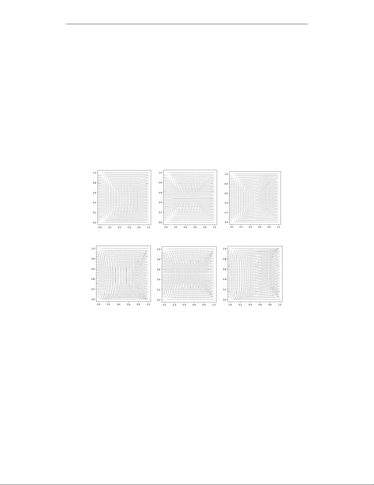
Defla tion-PINNs: Learning Mul tiple Solu- tions f or PDEs and Land a u-de Gennes Sean Disarò ∗ , R uma Rani Maity † , Aras Bac ho ‡ Abstra ct Nonlinear P artial Differential Equations (PDEs) are ubiquitous in mathemat- ical ph ysics and engineering. Although Ph ysics-Informed Neural Netw orks (PINNs) ha ve emerged as a p o werful to ol for solving PDE problems, they t ypically struggle to identify multiple distinct solutions, since they are de- signed to find one solution at a time. T o address this limitation, w e in tro duce Deflation-PINNs, a nov el framework that in tegrates a deflation loss with an arc hitecture based on PINNs and Deep Op erator Netw orks (DeepONets). By incorp orating a deflation term into the loss function, our meth o d sys- tematically forces the Deflation-PINN to seek and conv erge up on distinct finitely man y solution branc hes. W e pro vide theoretical evidence on the con vergence of our model and demonstrate the efficacy of Deflation-PINNs through numerical exp erimen ts on the Landau-de Gennes mo del of liquid crystals, a system renowned for its complex energy landscap e and multiple equilibrium states. Our results show that Deflation-PINNs can successfully iden tify and characterize multiple distinct crystal structures. Mathematics Sub ject Classification Ph ysics-Informed Machine Learning, Neural Net- w orks, DeepONets, Nonlinear Partial Differential Equations, Landau-de Gennes 1 Intr oduction P artial Differential Equations (PDEs) hav e a wide range of applications in many disciplines. Esp ecially in physics, all ma jor theories are formulated in the language of PDEs. How ev er, not all PDEs can b e solved analytically . Thus, it is imp ortan t to improv e and provide new n umerical metho ds to find approximated solutions for PDEs, making it p ossible to apply these solutions in engineering and other scientific fields. With increasing computational p o w er and with the rise of machine learning, there hav e b een great ideas for solving PDEs with neural netw orks. Suc h metho ds include the Deep Ritz metho d E and Y u ( 2017 ), the Deep Galerkin metho d Sirignano and Spiliop oulos ( 2018 ), Physics-Informed Neural Net w orks (PINNs) Raissi et al. ( 2019 ; 2017a ; b ); Lorenz et al. ( 2024 ), V ariational PINNs (VPINNs) Kharazmi et al. ( 2019 ) and Op erator Learning Li et al. ( 2021 ); Lu et al. ( 2021a ); Bac ho et al. ( 2025 ). A notoriously hard-to-compute field in which it is necessary to solve PDEs n umerically is the Landau-de Gennes (LdG) theory Ma jumdar and Zarnescu ( 2009 ), whic h is used to describ e liquid crystals. In this context, some formulations of problems hav e a discrete n umber of solutions, which represent liquid crystal structures. In this pap er, we will explore a new metho d, which is based on Physics-Informed Machine Learning (PIML) and which is designed to find solutions to an LdG problem, whic h was also in vestigated in Luo et al. ( 2012 ). Our framework is designed to b e fully unsup ervised and is designed to find all the solutions of the LdG problem at once. It works by combining a PIML loss with a nov el loss function, which ensures that the solutions found are distinct from each other. F urthermore, w e establish universalit y by constructing our architecture as a sp ecial case of DeepONets—a neural netw ork framew ork for learning op erators b et w een function spaces that is kno wn to b e univ ersal Lu et al. ( 2021a ); Chen and Chen ( 1995 ). With ∗ seandisaro@gmail.com † rumamait y081@gmail.com ‡ bac ho@caltech.edu 1 our approac h, we leverage the strengths of PINN framew orks to capture multiple solution branc hes of ODEs/PDEs. As argued in Zou et al. ( 2025 ), such coarse appro ximations are particularly v aluable when used as initializations for con ven tional n umerical solvers, which can subsequen tly refine them into high-precision solutions. 1.1 Rela ted Work There has already b een research which aims to find a finite num ber of solutions for a PDE. W e give a brief summary of related work. HomPINNs. In Zheng et al. ( 2024 ) the authors present the so-called Homotop y Physics- Informed Neural Netw orks (HomPINNs), which are similar to what we wan t. They are designed to allow for a discrete num ber of solutions for a PDE. Their approach, how ev er, aims to fit data from observ ations and additionally incorp orating a Physics-Informed loss in their total loss. Th us, this can b e viewed as a semi-sup ervised setting. Learning Multiple Solutions from Random Initializations. In Zou et al. ( 2025 ) the authors explore a different setting, in which they train man y conv en tional Physics-Informed Neural Net works (PINNs) and they initialize them with different random parameters in the hop e that through this random initialization, the optimization pro cess yields different solutions. Afterwards, the different solutions that w ere obtained w ere analyzed and compared to see which solution w as found how often. The adv antage of this approac h is that it is easily scalable as one can implement many PINNs in parallel. How ev er, since we cannot guaran tee that the different solutions the PINNs find are distinct, this approach is also v ery prone to redundancy and may lead to non-optimal use of resources. Neural Netw orks for Nematic Liquid Crystals. In Shi et al. ( 2024 ), the authors solv e a Landau-de Gennes problem with neural netw orks using a loss function based on an energy functional. How ever, unlik e our approac h, this approac h is not qualified to distinguish and find multiple solutions for an LdG problem. In Sigaki et al. ( 2020 ), the authors use Con volutional Neural Netw orks (CNNs), to learn prop erties ab out liquid crystals. As the use of CNNs suggests, this w ork uses images of liquid crystals as inputs to predict prop erties lik e the order parameter of simulated nematic liquid crystals. DeepONets. De ep Op er ator Networks (De epONets) are a neural netw ork framew ork for learning op erators b et ween function spaces. They were first in tro duced by Lu et al. ( 2021a ) and hav e since b een thoroughly studied in research. F or a brief introduction to DeepONets, w e refer to the app endix or to Lanthaler et al. ( 2022 ) for a detailed survey on DeepONets. 1.2 O ver view In Section 2 we briefly recall the concepts of physics-informed machine learning. Then we pro ceed with presen ting mo del architectures that are implemented with a hard constraint for Dirichlet conditions. In this context, we briefly discuss our metho d of doing so, by using radial extrap olation of functions. In the following Subsection 2.3 , we simplify the DeepONet architecture to fit our needs, and w e argue that, for our purposes, we still main tain univ ersality for the simplified mo del. More precisely , the simplified mo del will b e defined in a wa y that it can only approximate a fixed num ber of functions. Moreov er, we will in tro duce a new loss term, which mak es the different solutions, whic h we w an t to approximate with our mo del, distinguishable. W e call this new loss term Deflation loss and the total mo del will be called a Deflation-PINN . W e will also provide a theoretical analysis on the approximation capabilities of our new mo del. In the next section, we quic kly recall the Landau-de Gennes mo del and in tro duce the concrete problem which we wan t to solv e with our Deflation-PINN. W e compare the solutions found with the Finite Element Metho ds (FEMs) and rep ort the results. Finally , in the last section we give a brief discussion of the pap er. 2 2 Methodology In this section, we discuss the mo del that w e use in this pap er, and for this we will recall fundamen tal concepts including Ph ysics-Informed Machine Learning and neural netw orks with hard constraints. 2.1 Physics-Informed Machine Learning (PIML) The Idea of Physics-Informe d Machine L e arning (PIML) was first presented in Raissi et al. ( 2019 ). The goal is to enco de a PDE problem into a loss function, i.e let D [ u ]( x ) = 0 , for x ∈ Ω B [ u ]( s ) = ψ ( s ) , for s ∈ ∂ Ω , (2.1) where Ω ⊂ R d is compact and D , B are differen tial operators and b oundary op erators, u : Ω → R m , m ∈ N is the solution of the PDE, ψ : ∂ Ω → R m sp ecifies the boundary condition. Then we can define the gener alization err or for ( 2.1 ) as E G ( θ ) 2 := α 1 · Z Ω |D [ u θ ]( x ) | 2 dx + α 2 · Z ∂ Ω |B [ u θ ]( s ) − ψ ( s ) | 2 ds (2.2) where u θ is a trainable model parameterized b y θ in some parameter space Θ , and α 1 , α 2 are h yp erparameters. The PIML framework seeks to minimize the difference b et ween a mo del u θ and the actual solution u through the loss function ab o v e. In other words, if the solution to ( 2.1 ) is unique, then the generalization error is zero if and only if u θ = u . This is due to the fundamen tal lemma of the calculus of v ariation. When the mo del used is a neural netw ork, then the resp ectiv e neural netw ork with PIML loss is usually referred to as a Physics-Informe d Neur al Network (PINN) . T o actually compute the generalization error E G ( θ ) , we need to discretize it. The t ypical framew ork for this is to first discretize the differential op erators in R i [ f ]( x ) with automatic differen tiation (AD) Griewank and W alther ( 2008 ) and then discretize the integrals. F or the discretization of the integrals, one can use e.g. a Riemann sum. F or more literature on PIML, w e refer to Karniadakis et al. ( 2021 ); W ang et al. ( 2023 ). 2.2 Hard Constraints For Boundar y Conditions Usually , when a loss function consists of multiple ob jectiv es, e.g., such as the three in te- grals in E G , it is not trivial how to choose the resp ectiv e hyperparameter α i . This w as discussed in more detail in Escapil-Inchauspé and Ruz ( 2023 ); T oscano et al. ( 2024 ). In such m ulti-ob jectiv e loss functions, it is desirable to simplify the problem so that we ha ve fewer ob jectiv es to approximate. One w ay to achiev e this in the PINN framework is to adapt the architecture of the neural net work such that it automatically satisfies the b oundary conditions, and thus the general- ization error reduces to only E G ( θ ) 2 := R Ω |R i [ u θ ]( x ) | 2 dx. T o ensure this, we can c ho ose the follo wing ansatz. ˜ f θ ( x ) := ω ( x ) · N N θ ( x ) + b ( x ) ≈ u ( x ) where ω > 0 on the interior in t (Ω) and ω = 0 on ∂ Ω . b : ¯ Ω = ∂ Ω ∪ Ω → R should b e at least conti nuous and chosen so that b | ∂ Ω = ψ . N N θ ( x ) is a neural netw ork and the appro ximation is true for a suitable c hoice of parameters θ . Note that ˜ f θ satisfies the exact Diric hlet condition indep enden tly of the choice of θ . The exact imp osition of b oundary constraints has b een discussed extensively in literature; see Sukumar and Sriv asta v a ( 2022b ); Leake and Mortari ( 2020 ); Lu et al. ( 2021c ); T oscano et al. ( 2025 ). In this pap er, we use a custom extension which works in general on op en, b ounded star domains. The reason is that we found that this extension work ed well for our exp erimen ts. The extension is constructed radially with resp ect to the cen ter of the star domain. 3 So, let us assume that we hav e a b ounded, op en, and star-shap ed domain Ω ⊂ R d . W e can consider Ω in spherical co ordinates with center x 0 , i.e., for a p oin t x ∈ Ω , whic h is given in Cartesian co ordinates, we view this as x ∼ = ( φ x 0 x , θ x 0 x , r x 0 x ) := ( φ 0 x − x 0 , θ 0 x − x 0 , r 0 x − x 0 ) := ( φ x − x 0 , θ x − x 0 , || x − x 0 || 2 ) ∈ [ 0 , 2 π ) × [0 , π ) d − 2 × [0 , ∞ ) , where ( φ x − x 0 , θ x − x 0 , || x − x 0 || 2 ) ∈ [0 , 2 π ) × [0 , π ) d − 2 × [0 , ∞ ) is the usual represen tation of the p oin t x − x 0 in spherical co ordinates. Note that each b oundary p oin t x ∈ ∂ Ω corresp onds to one and only one angle in spherical co ordinates, i.e. ∂ Ω ← → [0 , 2 π ) × [0 , π ) d − 2 ← → S 1 × S d − 2 , where S n = ∂ B (0 , 1) ⊂ R n +1 denotes the b oundary of the unit ball in R n +1 . F urthermore, it is easy to see that these mappings are all contin uous. This gives rise to the following definition. Definition 1 L et Ω ⊂ R d b e a b ounde d, op en, and star-shap e d domain with r esp e ct to x 0 ∈ Ω . W e define the r adial b oundary distanc e function (RBD function) r Ω ,x 0 : ¯ Ω \ x 0 → [0 , ∞ ) of Ω with r esp e ct to x 0 , such that for al l x ∈ ¯ Ω \ { x 0 } we have r Ω ,x 0 ( x ) := || x b − x 0 || 2 . wher e x b ∈ ∂ Ω is such that x ∈ { (1 − t ) x 0 + tx b | t ∈ [0 , 1] } is in the line se gment c onne cting x b and x 0 . The definition is to b e understo o d so that every p oin t (except the center) is mapp ed radially to a b oundary p oin t, and the function returns the distance from the center to that b oundary p oin t, in particular w e hav e ( φ x 0 x , θ x 0 x ) = ( φ x 0 x b , θ x 0 x b ) . Example 2.1 The ball B ( x 0 , R ) ⊂ R d with radius R > 0 and center x 0 is a star-shap ed domain with resp ect to x 0 . Its RBD function is giv en by r B ( x 0 ,R ) ,x 0 : x 7→ R for all x ∈ ¯ B ( x 0 , R ) \ { x 0 } . No w, it is easy to define spherical contin uations in terms of the RBD function of a domain. Definition 2 L et Ω ⊂ R d b e a b ounde d, op en and star-shap e d domain with r esp e ct to x 0 and let r Ω ,x 0 b e a RBD function for Ω . L et h : [0 , 1] → [0 , 1] b e a c ontinuous function such that h | [0 , 1) > 0 , h (0) = 1 and h (1) = 0 . L et f ∈ C ( ∂ Ω) . Define ˜ ω ( x ) :      Ω → [ 0 , 1] x 7→ ( h ( || x − x 0 || r Ω ,x 0 ( x ) ) , if x  = x 0 0 , if x = x 0 . and ˜ f :  Ω → R x 7→ f ( φ x 0 x , θ x 0 x ) · (1 − ˜ ω ( x )) . Then ˜ ω, ˜ f ∈ C ( ¯ Ω) , we have ˜ ω = 0 on ∂ Ω and ˜ ω > 0 in int (Ω) and ˜ f | ∂ Ω = f . If we c ho ose h : [0 , 1] → [0 , 1] to b e smo oth and if Ω and f : ∂ Ω → R are smo oth, then ˜ ω and ˜ f are smo oth. The general difficulty of this approach is to find an RBD function for the domain, whic h is in general not easy . Note that ˜ ω satisfies the condition we need ab o v e for our ansatz. Ho wev er, we will not use this ˜ ω , but rather only ˜ f for the extrap olation of the b oundary function. F or ω w e will use the C ∞ − construction from Lu et al. ( 2021b ). 2.3 Defla tion-PINNs There are PDE problems, whic h hav e a finite num b er of solutions K > 1 . F or an example of suc h a problem, we refer to the section where we present our numerical results. Ho w ev er, this kind of problem is not cov ered b y the classical PINN framework, as it is only suitable for learning one solution at a time. Although the DeepONet framework can learn m ultiple solutions for a class of PDE problems, it is unlikely to b e the most efficient choice, since it is built to learn infinitely man y solutions in the form of an op erator b etw een function spaces. Th us, it may be seen as unnecessarily exp ensiv e if w e only wan t finitely man y solutions. This section introduces Deflation-PINNs , i.e. our new metho d for learning multiple solutions with neural net works. The metho d consists of tw o new k ey p oin ts. 4 1. W e will introduce a neural netw ork architecture to learn multiple solutions at the same time. The architecture will b e a sp ecial case of the DeepONet architecture but designed in such a wa y that it only admits a finite num ber of solutions. 2. W e will introduce a loss function that ensures that we learn different solutions for the same problem. 1) Architecture W e start with (unstac k ed) DeepONets, whic h w ant to appro ximate an op erator ov er a function space, i.e. they map G : A × R d → R , where A is a space of functions. The output then is of the form p P i =1 τ i ( x ) · β i ( f ) ≈ G ( f )( x ) where x ∈ R d and f ∈ A . The τ i are the outputs of a neural netw ork x 7→ ( τ 1 ( x ) , . . . , τ p ( x )) . The β i use the ev aluation of the function at previously fixed sensor p oin ts, that is, take ( ˜ x i ) N i =1 ∈ dom ( f ) sensor p oin ts, then f 7→ ( β 1 ( f ) , . . . , β p ( f )) = ( β 1 ( f ( ˜ x 1 , . . . , ˜ x N )) , . . . , β p ( f ( ˜ x 1 , . . . , ˜ x N ))) where β : R N → R p is a neural netw ork. Ho wev er, in our setting, we wan t to learn only K ∈ N solutions that do not dep end on an input function. Thus, w e prop ose, instead of using a neural netw ork β i : R N → R p , to use only K feature vectors of size p (one feature vector for each solution), which enco de the resp ectiv e function, i.e., we wan t β k = ( β k 1 , . . . , β k p ) ∈ R p . These feature vectors can then b e trained as part of the mo del’s parameters. In total, our solution is of the form ˜ G ( k , x ) := p X i =1 τ i ( x ) · β k i ≈ u k ( x ) , where x ∈ dom ( u k ) and u k for k = 1 , . . . , K are the K solutions w e w ant to appro ximate and τ i are still neural netw orks. An illustration of our prop osed arc hitecture is given in Figure 1 . Figure 1: Arc hitecture of the Deflation-PINN. The adv an tage of using fixed feature β k ∈ R p instead of neural netw orks β : A → R p is that w e only need K · p parameters to represen t the K functions. W e call the β k ∈ R p Branc h W eights . If we were to use the DeepONet arc hitecture, then we would need at least S · p + S parameters, where S ∈ N is the num b er of sensor p oints, whic h can easily b e greater than the num ber of solutions, that is, S > K . F urthermore, the K feature vector directly incorp orates the solution structure such that it can b e deco ded b y the architecture, since the feature vectors are trained to do so, which is in contrast to the fixed sensor p oints, whic h cannot b e changed. 5 Note that since we hav e a finite num b er of solutions, which we wan t to approximate for our arc hitecture, we still w ant to approximate a map of compact sets, and th us we can deriv e univ ersality for this architecture as a sp ecial case of theorem 2 . Corollary 1 Supp ose that σ : R → R is a c ontinuous and non-p olynomial activation function, X is a Banach function sp ac e, u 1 , . . . , u N ∈ X and K ⊂ R d c omp act. Then for al l ε > 0 ther e exists p ∈ N , ζ i ∈ R , ω i ∈ R d , such that for al l n ∈ { 1 , . . . , N } and y ∈ K we have that    u n ( y ) − p X i =1 β i n σ ( ω i · y + ζ i )    < ε. Pr o of. This is just a sp ecial case of theorem 2 2) Defla tion Loss W e now hav e an architecture for our problem, but the question remains how to train this. With the PIML loss, we can learn true solutions. How ev er, w e still need a loss, which tells the mo del that the K ∈ N solutions it learns (with the PIML loss) need to b e distinct from one another. Mor e precisely , the solutions u k that we wan t to approximate hav e to b e at least d min := min i,j ∈{ 1 ,...,K } ,i  = j || u i − u j || L 2 apart. Let ˜ G with ˜ G ( k , x ) := p X i =1 τ i ( x ) · β k i ≈ u k ( x ) b e our mo del. W e can rewrite the condition that the solutions b e at least d min apart as the follo wing loss function: L Def ( ˜ G ) := 2 K · ( K − 1) K X i =1 K X j = i +1 max  1 − 1 d min || ˜ G ( i, · ) − ˜ G ( j, · ) || L 2 , 0  , i.e., the resp ectiv e approximated solutions G ( i, · ) ha ve at least distance d min b et w een each other in the L 2 -norm if and only if L Def ( ˜ G ) = 0 . Th us, the total loss for training our mo del ˜ G can b e given as L total ( ˜ G ) := α · K X i =1 E G ( ˜ G ( i, · )) + β · L Def ( ˜ G ) where E G is the PIML generalization error and for some hyperparameters α, β > 0 . W e call this mo del ˜ G together with the loss function L total a Deflation-PINN . d min is left as a hyperparameter which can b e found empirically b y testing different v alues or by some theoretical b ound on the distance b et ween solutions. Figure 1 illustrates the architecture. 3) Hard Constraints Appro xima tion Theor y Appro ximation theory for mo dels with hard constraints is a topic which has already b een discussed in literature; see e.g. Sukumar and Sriv asta v a ( 2022a ), where the authors use the framew ork of R-functions, to establish a strong theoretical framework. Since we will also use hard constraints in the mo del for our exp erimen ts later, w e wan t to inv est a small section of this pap er as w ell into justifying the use of suc h hard constraint mo dels as describ ed in section 2.2 , via a nov el elemen tary theorem. The theorem is formulated in the ∥·∥ ∞ -top ology on the contin uous functions, which makes it applicable in com bination with corollary 1 . Theorem 1 A ssume Ω ⊂ R d is an op en domain. L et g , h ∈ C ( ¯ Ω ) , s.t. h | ∂ Ω = 0 and g > 0 on Ω , then ther e exists a se quenc e of functions ( f n ) n ∈ N ⊂ C ( ¯ Ω) , s.t. ∥ f n g − h ∥ Ω = ∥ f n g − h ∥ ∞ , Ω n →∞ − − − − → 0 W e now apply the theorem ab o ve onto our Deflation-PINN architecture: 6 Corollary 2 Supp ose that σ : R → R is a c ontinuous and non-p olynomial activation function, Ω ⊂ R d is c omp act, u 1 , . . . , u N ∈ C ( ¯ Ω ) , g , h ∈ C ( ¯ Ω ) s.t. h | ∂ Ω = u n for n ∈ { 1 , . . . , N } and g | ∂ Ω = 0 . Then for al l ε > 0 ther e exists p ∈ N , ζ i ∈ R , ω i ∈ R d , such that for al l n ∈ { 1 , . . . , N } and y ∈ K we have that    u n ( y ) −  h ( y ) − g ( y ) · p X i =1 β i n σ ( ω i · y + ζ i )     < ε. Pr o of. Fix ε > 0 . F rom theorem 1 we get for each n ∈ { 1 , . . . , N } a f ε,n ∈ C ∞ suc h that ∥ f ε,n · g − h ∥ Ω < ε. Then all need to do is to apply corollary 1 and approximate eac h f ε,n suc h that    f ε,n ( y ) − p X i =1 β i n σ ( ω i · y + ζ i )    < ε for all y ∈ K . The rest follows from the triangle inequality . 3 Numerical Experiments In this section, we discuss numerical results on the benchmark example of the reduced t wo-dimensional LdG mo del of liquid crystal theory , and presen t the solutions obtained through our Deflation-PINN. The co de can b e found in https://github.com/SeanDisaro/ DeflationPINNs . 3.1 Landa u-De Gennes Model Landau-de Gennes theory is a phenomenological v ariational theory that describes the state of nematic liquid crystals in terms of an order parameter, Q tensor. In t w o dimensions, Q tensor is a symmetric traceless matrix in R 2 × 2 , and is represented as a vector Q := ( Q 11 , Q 12 ) . In the absence of surface effects and external field, the reduced tw o dimensional LdG Luo et al. ( 2012 ) functional in the dimensionless form is given by E ( Q ) = Z Ω ( |∇ Q | 2 + ϵ − 2 ( | Q | 2 − 1) 2 ) dx , (3.1) where Q ∈ H 1 (Ω) and ϵ is a small parameter that dep ends on the elastic constant, the bulk energy parameters, and the domain size. W e are concerned with the minimization of the functional E ( • ) for the Lipschitz contin uous b oundary function Q b : ∂ Ω → R 2 consisten t with the exp erimen tally imp osed tangen t b oundary conditions. The energy formulation in ( 3.1 ) seeks Q ∈ H 1 (Ω) suc h that − ∆ Q = 2 ϵ − 2 (1 − | Q | 2 ) Q in Ω and Q = Q b on ∂ Ω . (3.2) F or our experiment, we use ϵ = 0 . 02 . W e solv e the system ( 3.2 ) in Ω := [0 , 1] × [0 , 1] with the Diric hlet b oundary condition Q b constructed utilizing trap ezoidal shap e function T d : [0 , 1] → R with d = 3 ϵ as Q b =  ( T d ( x ) , 0) on y = 0 and y = 1 , ( − T d ( y ) , 0) on x = 0 and x = 1 , and T d ( t ) =    t/d, 0 ≤ t ≤ d, 1 , d ≤ t ≤ 1 − d, (1 − t ) /d, 1 − d ≤ t ≤ 1 . Exp erimen tal and numerical inv estigations suggest that there are six stable solutions to this problem on a square domain, which hav e b een computed using FEMs; see T sakonas et al. ( 2007 ); Luo et al. ( 2012 ); Maity et al. ( 2021a ). T wo classes of stable exp erimen tally observ able configurations are rep orted: diagonal states (D1 and D2) in whic h the nematic directors are aligned along the square diagonals, and rotated states (R1, R2, R3, R4) in whic h the nematic directors rotate in π radian angles across the square edges. Some of these nematic equillibria are presented in Figure 2 . 7 3.2 Reproducibility St a tement The exp erimen ts were p erformed on an R TX 3060-Ti GPU with 8GB VRAM. W e use the mo del discussed in Section 2.3 with a hard constraint for the Dirichlet b oundary condition. The mo del is adapted to incorp orate tw o outputs, i.e. the final mo del G = ( G 1 , G 2 ) is of the form G 1 := ˜ G 1 ( k , x ) · ω ( x ) + ˜ Q b ( x ) = ω ( x ) · p X i =1 τ i ( x ) · β k i + ˜ Q b ( x ) ≈ u 1 k ( x ) G 2 := ˜ G 2 ( k , x ) · ω ( x ) = ω ( x ) · 2 p X i = p +1 τ i ( x ) · β k i ≈ u 2 k ( x ) , where β k ∈ R p for k = 1 , . . . 6 and τ : R 2 → R p is a neural netw ork with skip connections. ˜ G = ( ˜ G 1 , ˜ G 2 ) is the Deflation-PINN mo del of Section 2.3 without the hard constraint for t wo outputs. ω : [0 , 1] 2 → R is such that ω > 0 on (0 , 1) 2 and ω = 0 on ∂ [0 , 1] 2 . ˜ Q b ( x ) is an extension of the trap ezoidal function used in Q b and is given by ˜ Q b ( x ) | ∂ [0 , 1] 2 = Q 1 b =  T d ( x ) on y = 0 and y = 1 , − T d ( y ) on x = 0 and x = 1 . Note that we did not add anything to the second output term of the mo del and multiplied it only by ω . This is b ecause we require the Dirichlet condition to b e zero for the second term. Concretely , we use the C ∞ − construction from Lu et al. ( 2021b ) for ω and for ˜ Q b ( x ) we use the radial extension from Definition 2 , as describ ed in Section 2.2 . F or this, we use the p oin t ( 1 2 , 1 2 ) ∈ Ω := [0 , 1] 2 as a center for our star domain. The exact formula for the RBD function can b e explicitly calculated and for this w e refer to our implementation in our rep ository https://github.com/SeanDisaro/DeflationPINNs . F or the function h : [0 , 1] → [0 , 1] from Definition 2 we simply use the function h ( x ) = 1 − x , since this is v ery efficient to compute. Regarding the PIML loss function, we only need to implement the dynamics of the mo del since we already satisfy the Dirichlet condition b y construction. Thus, we can use equation ( 3.2 ) to formulate a generalization error of the form E G ( G ) := Z Ω   ϵ 2 · ∆ G 1 + 2 · (1 − G 1 · G 1 − G 2 · G 2 ) · G 1   dx + Z Ω   ϵ 2 · ∆ G 2 + 2 · (1 − G 1 · G 1 − G 2 · G 2 ) · G 2   dx . W e ev aluated the PIML loss on collo cation p oin ts on a 33 × 33 -grid and to ok the Riemann sum for this grid. The grid cov ers the domain [0 + δ, 1 − δ ] 2 . The safety distance is to facilitate training, and we can do this safely , as the b oundary condition is enforced. Regarding the deflation loss, w e use an additional trick. Instead of computing the L 2 ([0 , 1] 2 , R 2 ) norm for the mo del G ( i, · ) : R 2 → R 2 , whic h is suggested by how we in- tro duced the deflation loss in Section 2.3 , w e only compute the L 2 ([0 , 1] 2 , R ) norm for our second comp onen t. There is no particular reason why we chose the second comp onen t, but the adv an tage of only using one comp onent is that we mak e the computation of the deflation loss more efficient. Additionally , this simpler form has sho wn to facilitate the training process in our exp erimen ts. W e used d min = 0 . 4 . This parameter was found empirically through testing and was not computed analytically . This was done by chec king if the solutions after training were to o similar (in which case we increased d min ) and, on the other hand, if the PIML term did not con verge, then we decreased d min . Th us, the deflation loss we used is given by L Def ( G ) := 1 15 6 X i =1 6 X j = i +1 max  1 − 5 2 || G 2 ( i, · ) − G 2 ( j, · ) || L 2 ([0 , 1] 2 , R ) , 0  . T o compute the L 2 ([0 , 1] 2 , R ) norm for the deflation loss, we use the same grid / collo cation p oin ts, as for the PIML loss. The total loss is of the form L total ( G ) := α · 6 X i =1 E G ( G ( i, · )) + β · L Def ( G ) 8 (a) Q N N D1 (b) Q N N R1 (c) Q N N R3 (d) Q F E M D1 (e) Q F E M R1 (f ) Q F E M R3 Figure 2: V ector field plots of one diagonal and t wo rotated solutions, denoted by D1, R1 and R3 in suffix, with Deflation PINNs and FEM. and w e used α = 0 . 02 and β = 2 . In our exp erimen ts, we use the A dam optimizer to train for 10 , 000 ep o c hs with an initial learning rate of 1 · 10 − 3 . τ : R 2 → R p is of width 4000 and has one lay er. W e use tanh as the activ ation function. W e set the output size of τ and the size of the representation v ectors to p = 16 . W e compare our results with the results from Maity et al. ( 2021b ), which were calculated using the finite element metho d and the results can b e seen in table 2 and table 4 . 4 Discussion In this pap er, we discuss a Deflation-PINNs for solving nonlinear PDEs with a discrete n umber of solutions. W e based our approach on w ell established mo dels such as PINNs and DeepONets. More precisely , we simplified the DeepONet arc hitecture so that it can only appro ximate a finite discrete num ber of solutions, and we augmented the PINN loss with a deflation loss so that if it is provided with multiple solutions, the mo del can distinguish b et w een differen t solutions. Contrary to other neural netw ork approac hes for finding multiple PDE solutions, w e do not rely on random initializations, and we show ed that the deflation loss provides a robust and systematic metho d for finding multiple solutions. This metho d w as tested on a Landau-de Gennes problem and it was able to detect all solutions, which could also b e detected with the classical finite element metho d. 9 5 A cknowledgments A.Bac ho ackno wledges supp ort from the Air F orce Office of Scientific Research (AFOSR) under aw ards F A9550-20-1-0358 (MURI: “Machine Learning and Physics-Based Modeling and Sim ulation”) and F A9550-24-1-0237, the U.S. Department of Energy (DOE), Office of Science, Office of Adv anced Scientific Computing Research (ASCR) under aw ard DE-SC0023163 (SEA-CR OGS: “Scalable, Efficient and A ccelerated Causal Reasoning Op erators, Graphs and Spikes for Earth and Embedded Systems”), and the Office of Nav al Research (ONR) under a ward N00014-25-1-2035. References A. Bacho, A. G. Sorokin, X. Y ang, T. Bourdais, E. Calvello, M. Darcy , A. Hsu, B. Hos- seini, and H. Owhadi. Operator learning at mac hine precision. In: arXiv pr eprint arXiv:2511.19980 , 2025. doi: 10.48550/arXiv.2511.19980. URL 2511.19980 . T. Chen and H. Chen. Univ ersal approximation to nonlinear op erators by neural netw orks with arbitrary activ ation functions and its application to dynamical systems. IEEE T r ansactions on Neur al Networks , 6(4):911–917, 1995. doi: 10.1109/72.392253. W. E and B. Y u. The deep ritz metho d: A deep learning-based numerical algorithm for solving v ariational problems. CoRR , abs/1710.00211, 2017. URL abs/1710.00211 . P . Escapil-Inchauspé and G. A. Ruz. Hyper-parameter tuning of physics-informed neu- ral netw orks: Application to helmholtz problems. Neur o c omputing , 561:126826, 2023. ISSN 0925-2312. doi: https://doi.org/10.1016/j.neucom.2023.126826. URL https: //www.sciencedirect.com/science/article/pii/S0925231223009499 . A. Griewank and A. W alther. Evaluating Derivatives . Society for Industrial and Applied Mathematics, second edition, 2008. URL https://epubs.siam.org/doi/abs/10.1137/ 1.9780898717761 . G. E. Karniadakis, I. G. Kevrekidis, L. Lu, P . Perdikaris, S. W ang, and L. Y ang. Physics- informed mac hine learning. Natur e R eviews Physics , 3(6):422–440, Jun 2021. ISSN 2522-5820. URL https://doi.org/10.1038/s42254- 021- 00314- 5 . E. Kharazmi, Z. Zhang, and G. E. Karniadakis. V ariational ph ysics-informed neural netw orks for solving partial differen tial equations. CoRR , 2019. URL 1912.00873 . S. Lanthaler, S. Mishra, and G. E. Karniadakis. Error estimates for deep onets: A deep learning framew ork in infinite dimensions, 2022. URL . C. Leake and D. Mortari. Deep theory of functional connections: A new method for estimating the solutions of partial differential equations. Machine L e arning and K now le dge Extr action , 2(1):37–55, Mar. 2020. ISSN 2504-4990. URL http://dx.doi.org/10.3390/ make2010004 . Z. Li, N. B. Ko v ac hki, K. Azizzadenesheli, B. Liu, K. Bhattachary a, A. M. Stuart, and A. Anandkumar. F ourier neural op erator for parametric partial differen tial equations. In 9th International Confer enc e on L e arning R epr esentations (ICLR 2021) . Op enReview.net, 2021. URL https://openreview.net/forum?id=c8P9NQVtmnO . B. Lorenz, A. Bac ho, and G. Kutyniok. Error estimation for ph ysics-informed neural netw orks appro ximating semilinear wa ve equations. 2024. URL 07153 . L. Lu, P . Jin, G. Pang, Z. Zhang, and G. E. Karniadakis. Learning nonlinear op erators via deep onet based on the universal approximation theorem of op erators. Natur e Machine Intel ligenc e , 3(3):218–229, Mar. 2021a. ISSN 2522-5839. doi: 10.1038/s42256- 021- 00302- 5. URL http://dx.doi.org/10.1038/s42256- 021- 00302- 5 . 10 L. Lu, X. Meng, Z. Mao, and G. E. Karniadakis. DeepXDE: A deep learning library for solving differential equations. SIAM R eview , 63(1):208–228, 2021b. URL https: //doi.org/10.1137/19M1274067 . L. Lu, R. Pestourie, W. Y ao, Z. W ang, F. V erdugo, and S. G. Johnson. Ph ysics-informed neural net works with hard constraints for inv erse design. SIAM Journal on Scientific Computing , 43(6):B1105–B1132, 2021c. URL https://doi.org/10.1137/21M1397908 . C. Luo, A. Ma jumdar, and R. Erban. Multistabilit y in planar liquid crystal wells. Physics R eview E , 85:061702, Jun 2012. URL https://link.aps.org/doi/10.1103/PhysRevE. 85.061702 . R. R. Maity , A. Ma jumdar, and N. Natara j. Discontin uous Galerkin finite elemen t metho ds for the Landau-de Gennes minimization problem of liquid crystals. IMA J. Numer. A nal. , 41(2): 1130–1163, 2021a. ISSN 0272-4979. URL https://doi.org/10.1093/imanum/draa008 . R. R. Maity , A. Ma jumdar, and N. Natara j. Parameter dep enden t finite element analysis for ferronematics solutions. Comput. Math. Appl. , 103:127–155, 2021b. ISSN 0898-1221. URL https://doi.org/10.1016/j.camwa.2021.10.027 . A. Ma jumdar and A. Zarnescu. Landau–de gennes theory of nematic liquid crystals: the oseen–frank limit and b ey ond. A r ch. R ation. Me ch. A nal , 196(1):227–280, July 2009. ISSN 1432-0673. URL http://dx.doi.org/10.1007/s00205- 009- 0249- 2 . M. Raissi, P . Perdikaris, and G. E. Karniadakis. Ph ysics informed deep learning (part i): Data-driv en solutions of nonlinear partial differen tial equations, 2017a. URL https: //arxiv.org/abs/1711.10561 . M. Raissi, P . Perdikaris, and G. E. Karniadakis. Ph ysics informed deep learning (part ii): Data-driv en discov ery of nonlinear partial differential equations, 2017b. URL https: //arxiv.org/abs/1711.10566 . M. Raissi, P . Perdikaris, and G. Karniadakis. Ph ysics-informed neural netw orks: A deep learning framew ork for solving forward and inv erse problems inv olving nonlinear partial differen tial equations. J. Comput. Phys. , 378:686–707, 2019. ISSN 0021-9991. URL https://www.sciencedirect.com/science/article/pii/S0021999118307125 . B. Shi, A. Ma jumdar, and L. Zhang. Neural netw ork-based tensor mo del for nematic liquid crystals with accurate microscopic information, 2024. URL 2411.12224 . H. Y. D. Sigaki, E. K. Lenzi, R. S. Zola, M. Perc, and H. V. Rib eiro. Learning phys- ical properties of liquid crystals with deep conv olutional neural net w orks. Scientific R ep orts , 10(1):7664, May 2020. ISSN 2045-2322. URL https://doi.org/10.1038/ s41598- 020- 63662- 9 . J. Sirignano and K. Spiliop oulos. Dgm: A deep learning algorithm for solving partial differen tial equations. Journal of Computational Physics , 375:1339–1364, Dec. 2018. ISSN 0021-9991. URL http://dx.doi.org/10.1016/j.jcp.2018.08.029 . N. Sukumar and A. Sriv asta v a. Exact imp osition of b oundary conditions with dis- tance functions in ph ysics-informed deep neural netw orks. Computer Metho ds in Ap- plie d Me chanics and Engine ering , 389:114333, 2022a. ISSN 0045-7825. URL https: //www.sciencedirect.com/science/article/pii/S0045782521006186 . N. Sukumar and A. Sriv asta v a. Exact imp osition of b oundary conditions with distance functions in physics-informed deep neural netw orks. Comput. Metho ds Appl. Me ch. Eng. , 389:114333, 2022b. ISSN 0045-7825. URL https://www.sciencedirect.com/science/ article/pii/S0045782521006186 . J. D. T oscano, T. Käufer, Z. W ang, M. Maxey , C. Cierpka, and G. E. Karniadakis. Inferring turbulen t velocity and temp erature fields and their statistics from lagrangian velocity measuremen ts using ph ysics-informed kolmogoro v-arnold netw orks, 2024. URL https: //arxiv.org/abs/2407.15727 . 11 J. D. T oscano, V. Oommen, A. J. V arghese, Z. Zou, N. Ahmadi Daryak enari, C. W u, and G. E. Karniadakis. F rom pinns to pikans: recen t adv ances in ph ysics-informed machine learning. Machine L e arning for Computational Scienc e and Engine ering , 1(1):15, Mar 2025. ISSN 3005-1436. URL https://doi.org/10.1007/s44379- 025- 00015- 1 . C. T sakonas, A. J. Davidson, C. V. Bro wn, and N. J. Mottram. Multistable alignmen t states in nematic liquid crystal filled wells. A pplie d Physics L etters , 90:Article 111913, 2007. URL 10.1063/1.2713140 . S. W ang, S. Sankaran, H. W ang, and P . Perdikaris. An exp ert’s guide to training physics- informed neural netw orks, 2023. URL . H. Zheng, Y. Huang, Z. Huang, W. Hao, and G. Lin. Hompinns: Homotopy physics- informed neural netw orks for solving the in verse problems of nonlinear differential equations with multiple solutions. J. Comput. Phys. , 500:112751, 2024. ISSN 0021-9991. URL https://www.sciencedirect.com/science/article/pii/S0021999123008471 . Z. Zou, Z. W ang, and G. E. Karniadakis. Learning and disco vering multiple solutions using ph ysics-informed neural netw orks with random initialization and deep ensemble, 2025. URL . 12 A Theorems and Pr oofs Theorem 2 ( Chen and Chen ( 1995 )) Supp ose that • σ : R → R is c ontinuous and non-p olynomial activation function, • X is a Banach sp ac e, • K 1 ⊂ X , K 2 ⊂ R d ar e b oth c omp act, • V ⊂ C ( K 1 ) is c omp act, • G : V → C ( K 2 ) b e a c ontinuous (non-line ar) op er ator, then for al l ε > 0 ther e exists n, p, m ∈ N , c k i , ξ k ij , θ k i , ζ k ∈ R , ω k ∈ R d , x j ∈ K 1 such that for al l u ∈ V and y ∈ K 2 we have that    G ( u )( y ) − p X k =1 n X i =1 c k i σ  m X j =1 ξ k ij u ( x j ) + θ k i  σ ( ω k · y + ζ k )    < ε. Lemma 1 F or n ∈ R let N n ⊂ R d b e c omp act sets. A ssume that N n ⊃ N n +1 for al l n ∈ N and that N := S n ∈ N N n ⊂ R d is b ounde d. A ssume that h ∈ C ( ¯ N ) and h | T n ∈ N N n = 0 . Then ∥ h ∥ ∞ ,N n n →∞ − − − − → 0 Pr o of. Assume ∃ C > 0 s.t. ∀ n ∈ N : ∥ h ∥ ∞ ,N n > 0 . Then we find a sequence of p oin ts x n ∈ N n , s.t. | h ( x n ) | = sup x ∈ N n | h ( x ) | > C . ( x n ) n ∈ ℸ ⊂ N is a b ounded sequence. Bolzano W eierstrass gives us a con verging subsequence ( x n k ) k ∈ N and x 0 := lim k →∞ x n k ∈ T n ∈ N N n . Th us w e found a x 0 ∈ T n ∈ N N n s.t. h ( x 0 ) ≥ C > 0 . Theorem 3 A ssume Ω ⊂ R d is an op en domain. L et g , h ∈ C ( ¯ Ω ) , s.t. h | ∂ Ω = 0 and g > 0 on Ω , then ther e exists a se quenc e of functions ( f n ) n ∈ N ⊂ C ( ¯ Ω) , s.t. ∥ f n g − h ∥ Ω = ∥ f n g − h ∥ ∞ , Ω n →∞ − − − − → 0 Pr o of. Fix ε > 0 . W e b egin by defining for λ ≥ 0 A λ := { x ∈ Ω : dist ( x, ∂ Ω) > λ } A λ has the following prop erties: • A λ is op en for all λ ≥ 0 • ∃ λ > 0 s.t. A λ  = ∅ • If A λ  = ∅ , then A λ 2 ⊋ A λ No w we observe, that for a fix λ > 0 s.t. A λ  = ∅ if we define A n := A λ 2 n and N n := ¯ Ω \ A n w e hav e that ( N n ) n ∈ N fulfills the condition from lemma 1 ab o ve and thus we can find a n ∈ N s.t. ∥ h ∥ ∞ ,N n < ε . Now we fix this n and define  A := A n B := A n +1 Define the function f ( x ) = h ( x ) g ( x ) for x ∈ Ω . Note that f is contin uous on Ω , but 13 not necessarily contin uous on ¯ Ω . No w we take a con tinuous function φ ∈ C ( ¯ Ω ) , s.t. ∥ φ ∥ = 1 , φ = 1 on A and φ = 0 on ¯ Ω \ B . Define the function f ε := f · φ ∈ C 0 ( ¯ Ω) = { g ∈ C ( ¯ Ω) : g | ∂ Ω = 0 } ⊂ C ( ¯ Ω) . The follo wing simple estimate concludes the pro of: ∥ f ε g − h ∥ Ω ≤ ∥ f ε g − h ∥ A | {z } = ∥ ( f ε − f ) g ∥ A =0 + ∥ f ε g − h ∥ Ω \ A ≤ ∥ f ε g ∥ Ω \ A + ∥ h ∥ Ω \ A | {z } ≤ ε ≤ ∥ f φg ∥ Ω \ A + ε = ∥ f φg ∥ B \ A + ε ≤ ∥ f g ∥ B \ A + ε = ∥ h ∥ B \ A + ε ≤ ∥ h ∥ Ω \ A + ε ≤ 2 ε B DeepONets De ep Op er ator Networks (De epONets) are a neural netw ork framew ork for learning op erators b et w een function spaces. They are based on the classical approximation result for op erators b y Chen and Chen ( 1995 ). Theorem 4 ( Chen and Chen ( 1995 )) Supp ose that • σ : R → R is c ontinuous and non-p olynomial activation function, • X is a Banach sp ac e, • K 1 ⊂ X , K 2 ⊂ R d ar e b oth c omp act, • V ⊂ C ( K 1 ) is c omp act, • G : V → C ( K 2 ) b e a c ontinuous (non-line ar) op er ator, then for al l ε > 0 ther e exists n, p, m ∈ N , c k i , ξ k ij , θ k i , ζ k ∈ R , ω k ∈ R d , x j ∈ K 1 such that for al l u ∈ V and y ∈ K 2 we have that    G ( u )( y ) − p X k =1 n X i =1 c k i σ  m X j =1 ξ k ij u ( x j ) + θ k i  σ ( ω k · y + ζ k )    < ε. The fixe d p oints x j ar e c al le d sensor p oints . Lu et al. ( 2021a ) reused this idea to introduce what w e now know as DeepONets. Let us no w give a precise definition of DeepONets. This definition is b orrow ed from Lanthaler et al. ( 2022 ). Definition 3 L et D ⊂ R d b e a c omp act domain and m, p ∈ N . Define the fol lowing op er ators • Enc o der: Given a set of sensor p oints ( x j ) m j =1 ⊂ D , we define the line ar mapping  E : C ( D ) → R m , E ( u ) = ( u ( x 1 ) , . . . , u ( x m )) • A ppr oximator: Given the evaluation of the sensor p oints, the appr oximator is a neur al network, that maps A : R m → R p . The c omp osition A ◦ E is cal le d Br anch Net . 14 • R e c onstructor: W e intr o duc e a neur al network  τ : R n → R p +1 y 7→ ( τ 0 ( y ) , . . . , τ p ( y )) and c al l it the T runk Net . Then the r e c onstructor is define d as    R = R τ : R p → C ( U ) , α 7→ τ 0 ( · ) + p P k =1 α k τ k ( · ) . Then c al l the c omp osition of r e c onstructor and br anch net E ◦ A ◦ R a De epONet . In the original pap er Lu et al. ( 2021a ), the authors prop ose tw o different implementations of the approximator. The first is the unstacke d De epONet , where the approximator consists of only one neural netw ork, as in the ab o v e definition, and the second is the stacke d De epONet , where the approximator consists of one neural net work for each output feature. More precisely , we get A stack ed ( u 1 , . . . , u m ) = ( A 1 ( u 1 , . . . , u m ) , . . . , A p ( u 1 , . . . , u m )) where eac h A i : R m → R is a neural net work. Although this is the v ersion used in theorem 2 , the authors outline the drawbac ks in computational complexity of the stack ed v ersion and even show in their exp erimen tal findings that the unstack ed v ersion outp erforms the stac ked version in terms of total error. F urthermore, it can b e easily shown that we also get univ ersality for the unstack ed version, by using the fact that neural netw orks are universal appro ximators. F urthermore, for an extensive error analysis for DeepONets we refer to Lan thaler et al. ( 2022 ). C Figures And T ables (a) D1 (b) D2 (c) R1 (d) R2 (e) R3 (f ) R4 Figure 3: Diagonally stable molecular alignments: (a) D1, (b) D2 states and rotated stable molecular alignments: (c) R1, (d) R2, (e) R3, (f ) R4 states. See Maity et al. ( 2021a ) for more details. 15 (a) Q N N D2 (b) Q N N R2 (c) Q N N R4 (d) Q F E M D2 (e) Q F E M R2 (f ) Q F E M R4 Figure 4: V ector field plots of one diagonal and t wo rotated solutions, denoted by D1, R1 and R3 in suffix, with Deflation PINNs and FEM. 16