GEAKG: Generative Executable Algorithm Knowledge Graphs

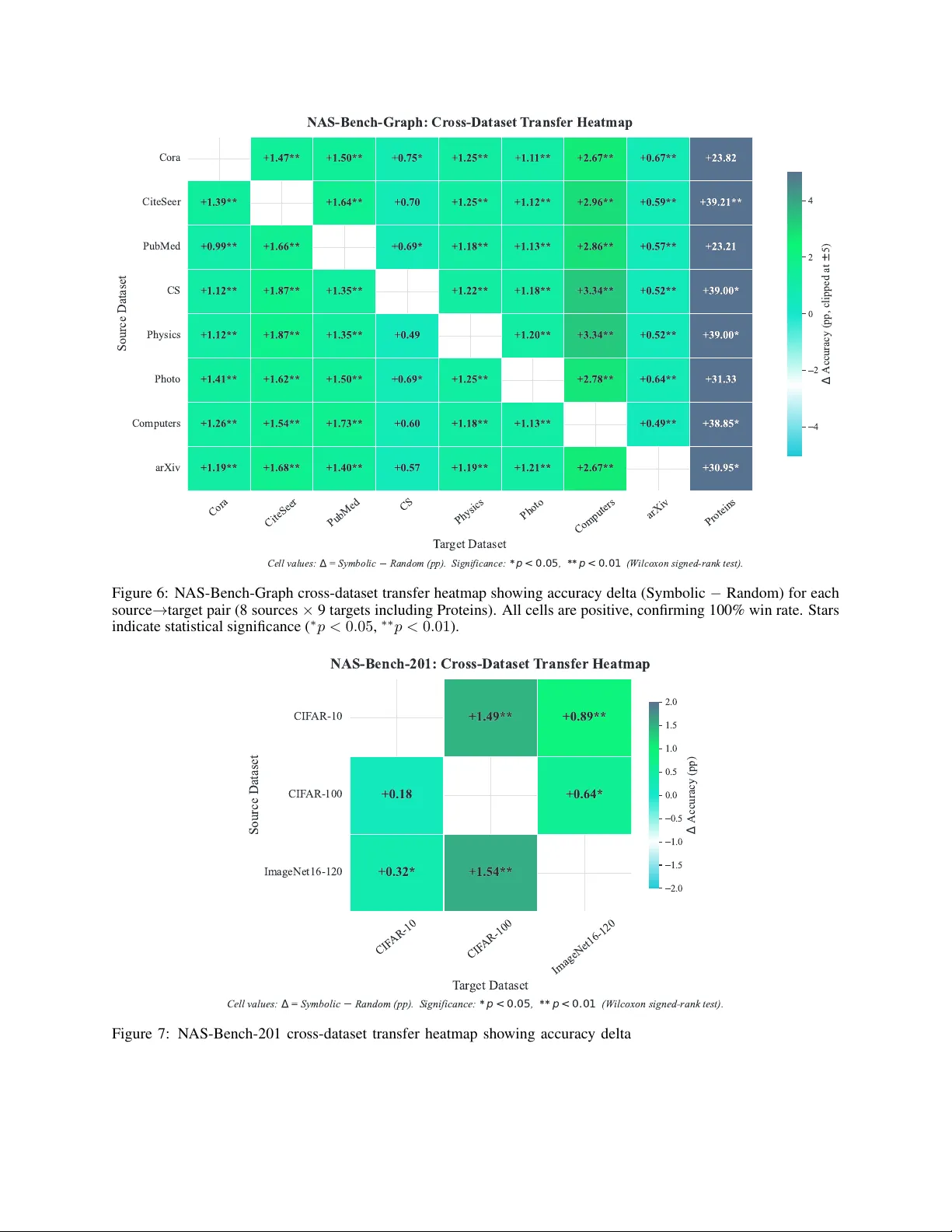
G E A K G : G E N E R A T I V E E X E C U T A B L E A L G O R I T H M K N O W L E D G E G R A P H S Camilo Chac ´ on Sartori ∗ Catalan Institute of Nanoscience and Nanotechnology (ICN2), CSIC and BIST , Campus U AB, Bellaterra, Barcelona, Spain camilo.chacon@icn2.cat Jos ´ e H. Garc ´ ıa Catalan Institute of Nanoscience and Nanotechnology (ICN2), CSIC and BIST , Campus U AB, Bellaterra, Barcelona, Spain josehugo.garcia@icn2.cat Andrei V oicu T omut Catalan Institute of Nanoscience and Nanotechnology (ICN2), CSIC and BIST , Campus U AB, Bellaterra, Barcelona, Spain andrei.tomut@icn2.cat Christian Blum Artiﬁcial Intelligence Research Institute (IIIA-CSIC), Bellaterra, Spain christian.blum@iiia.csic.es A B S T R AC T In the context of algorithms for problem solving, procedural knowledge—the kno w-how of algo- rithm design and operator composition—remains implicit in code, lost between runs, and must be re-engineered for each new domain. Knowledge graphs (KGs) have prov en effecti ve for organizing declarativ e kno wledge, yet current KG paradigms pro vide limited support for representing procedu- ral kno wledge as ex ecutable, learnable graph structures. W e introduce Generative Executable Algo- rithm Knowledge Graphs (GEAKG), a class of KGs whose nodes store e xecutable operators, whose edges encode learned composition patterns, and whose traversal generates solutions. A GEAKG is generative (topology and operators are synthesized by a Lar ge Language Model), executable (e very node is runnable code), and transferable (learned patterns generalize zero-shot across domains). The framew ork is domain-agnostic at the engine lev el: the same three-layer architecture and Ant Colon y Optimization (A CO)-based learning engine can be instantiated across domains, parameterized by a pluggable ontology ( RoleSchema ). T wo case studies—sharing no domain-speciﬁc framework code—provide concrete evidence for this framework hypothesis: (1) Neural Architecture Search across 70 cross-dataset transfer pairs on two tabular benchmarks, and (2) Combinatorial Optimiza- tion, where knowledge learned on the T raveling Salesman Problem transfers zero-shot to scheduling and assignment domains. T aken together , the results support that algorithmic expertise can be ex- plicitly represented, learned, and transferred as ex ecutable knowledge graphs. K eywords Procedural Knowledge Graphs, Generati ve Ex ecutable Algorithm Kno wledge Graphs, Knowledge Reuse, Automated Algorithm Design, Neural Architecture Search, Combinatorial Optimization. ∗ Corresponding author . GEAKG: Generative Executable Algorithm Knowledge Gr aphs Contents 1 Introduction 4 2 Related W ork 6 2.1 Automated Algorithm Design . . . . . . . . . . . . . . . . . . . . . . . . . . . . . . . . . . . . . . . 6 2.2 Knowledge Graphs and Ex ecutable Knowledge . . . . . . . . . . . . . . . . . . . . . . . . . . . . . 6 2.3 Neural Architecture Search . . . . . . . . . . . . . . . . . . . . . . . . . . . . . . . . . . . . . . . . 7 2.4 Neuro-Symbolic Integration . . . . . . . . . . . . . . . . . . . . . . . . . . . . . . . . . . . . . . . 7 3 The GEAKG Framework 7 3.1 The RoleSchema Abstraction . . . . . . . . . . . . . . . . . . . . . . . . . . . . . . . . . . . . . . . 10 3.2 Abstract Roles as Ontological Primitiv es . . . . . . . . . . . . . . . . . . . . . . . . . . . . . . . . . 11 3.3 Layer L0: MetaGraph T opology (Of ﬂine, LLM) . . . . . . . . . . . . . . . . . . . . . . . . . . . . . 12 3.4 Layer L1: Operator Generation (Ofﬂine, LLM) . . . . . . . . . . . . . . . . . . . . . . . . . . . . . 12 3.5 Layer L2: Learned Knowledge (Of ﬂine, A CO) . . . . . . . . . . . . . . . . . . . . . . . . . . . . . . 13 3.5.1 GEAKG Snapshot . . . . . . . . . . . . . . . . . . . . . . . . . . . . . . . . . . . . . . . . 13 3.6 Ofﬂine Phase: T raining Pipeline . . . . . . . . . . . . . . . . . . . . . . . . . . . . . . . . . . . . . 14 3.7 L2 T raining: Graph-Based Knowledge Acquisition (Of ﬂine) . . . . . . . . . . . . . . . . . . . . . . 14 3.8 Connection to KG Rule Learning . . . . . . . . . . . . . . . . . . . . . . . . . . . . . . . . . . . . . 14 3.9 Online Phase: Symbolic Execution . . . . . . . . . . . . . . . . . . . . . . . . . . . . . . . . . . . . 14 3.10 Domain Instantiation via CaseStudy . . . . . . . . . . . . . . . . . . . . . . . . . . . . . . . . . . . 15 3.11 Domain Abstraction: A T wo-T ier Protocol . . . . . . . . . . . . . . . . . . . . . . . . . . . . . . . . 15 3.12 Putting It T ogether: A T oy Example . . . . . . . . . . . . . . . . . . . . . . . . . . . . . . . . . . . 15 4 Domain Instantiation: T wo Case Studies 16 4.1 Case Study 1: Neural Architecture Search . . . . . . . . . . . . . . . . . . . . . . . . . . . . . . . . 16 4.2 Case Study 2: Combinatorial Optimization . . . . . . . . . . . . . . . . . . . . . . . . . . . . . . . . 17 4.3 Why the GEAKG Architecture W orks . . . . . . . . . . . . . . . . . . . . . . . . . . . . . . . . . . 18 5 Knowledge T ransfer and Integration 18 5.1 T ransfer T axonomy . . . . . . . . . . . . . . . . . . . . . . . . . . . . . . . . . . . . . . . . . . . . 18 5.2 Cross-Domain T ransfer via GEAKG (Case Study 2) . . . . . . . . . . . . . . . . . . . . . . . . . . . 18 5.2.1 T ransfer Mechanism and Scope . . . . . . . . . . . . . . . . . . . . . . . . . . . . . . . . . 18 5.3 Cross-Dataset T ransfer via GEAKG (Case Study 1) . . . . . . . . . . . . . . . . . . . . . . . . . . . 19 5.4 Side-Effect: Integration with Code-Ev olution Methods . . . . . . . . . . . . . . . . . . . . . . . . . 19 6 Experimental Setup 20 6.1 Common Experimental Protocol . . . . . . . . . . . . . . . . . . . . . . . . . . . . . . . . . . . . . 20 6.2 Case Study 2: Optimization — Experimental Setup . . . . . . . . . . . . . . . . . . . . . . . . . . . 21 6.2.1 Pure Mode: Representation-Based Generic Operators . . . . . . . . . . . . . . . . . . . . . . 21 6.2.2 Benchmark Instances . . . . . . . . . . . . . . . . . . . . . . . . . . . . . . . . . . . . . . . 21 2 GEAKG: Generative Executable Algorithm Knowledge Gr aphs 6.2.3 Problem Domains and Instances . . . . . . . . . . . . . . . . . . . . . . . . . . . . . . . . . 21 6.3 Case Study 1: N AS — Experimental Setup . . . . . . . . . . . . . . . . . . . . . . . . . . . . . . . 22 7 Results 22 7.1 Case Study 2: Optimization — Results . . . . . . . . . . . . . . . . . . . . . . . . . . . . . . . . . . 23 7.1.1 GEAKG-pure vs LLaMEA on TSP (Multi-LLM) . . . . . . . . . . . . . . . . . . . . . . . . 23 7.1.2 Local SLM Stress-T est (Qwen2.5-14B) . . . . . . . . . . . . . . . . . . . . . . . . . . . . . 23 7.1.3 Summary: Success Rate by Conﬁguration . . . . . . . . . . . . . . . . . . . . . . . . . . . . 24 7.1.4 Cross-Domain T ransfer (RQ2 + RQ3) . . . . . . . . . . . . . . . . . . . . . . . . . . . . . . 24 7.1.5 T ransfer Cost Analysis . . . . . . . . . . . . . . . . . . . . . . . . . . . . . . . . . . . . . . 25 7.1.6 Hybrid GEAKG (Embedded LLaMEA) vs Standalone LLaMEA (50k) . . . . . . . . . . . . 26 7.1.7 Ablation: Architecture vs Operator Quality . . . . . . . . . . . . . . . . . . . . . . . . . . . 26 7.2 Case Study 1: N AS — Results . . . . . . . . . . . . . . . . . . . . . . . . . . . . . . . . . . . . . . 26 7.2.1 Does the GEAKG Guide Effecti ve Architecture Search? . . . . . . . . . . . . . . . . . . . . 27 7.2.2 Generality Across Architecture Families (RQ1) . . . . . . . . . . . . . . . . . . . . . . . . . 28 7.2.3 Cross-Dataset T ransfer (RQ2) . . . . . . . . . . . . . . . . . . . . . . . . . . . . . . . . . . 28 7.2.4 Symbolic Executor: Transfer at Zero Cost (RQ3) . . . . . . . . . . . . . . . . . . . . . . . . 30 8 Analysis of the Learned GEAKG as a Knowledge Artifact 31 8.1 Structural Properties of the Learned Graph . . . . . . . . . . . . . . . . . . . . . . . . . . . . . . . . 31 8.2 Pheromone Con ver gence as Knowledge Reﬁnement . . . . . . . . . . . . . . . . . . . . . . . . . . . 32 8.3 Symbolic Rules: Learned Inference ov er the Procedural Graph . . . . . . . . . . . . . . . . . . . . . 32 8.4 Dominant Paths: Procedural Knowledge Patterns . . . . . . . . . . . . . . . . . . . . . . . . . . . . 34 9 Discussion 34 9.1 GEAKG as a General Procedural Knowledge Graph . . . . . . . . . . . . . . . . . . . . . . . . . . . 34 9.2 Knowledge Quality Assurance via Generation–V alidation Separation . . . . . . . . . . . . . . . . . . 35 9.3 Integration with Code-Ev olution Methods . . . . . . . . . . . . . . . . . . . . . . . . . . . . . . . . 35 9.4 Implications for Knowledge-Based Systems . . . . . . . . . . . . . . . . . . . . . . . . . . . . . . . 36 9.5 Reasoning and Queries ov er Procedural KGs . . . . . . . . . . . . . . . . . . . . . . . . . . . . . . . 36 9.6 Limitations and Threats to V alidity . . . . . . . . . . . . . . . . . . . . . . . . . . . . . . . . . . . . 37 9.7 Future W ork . . . . . . . . . . . . . . . . . . . . . . . . . . . . . . . . . . . . . . . . . . . . . . . . 38 10 Conclusion 38 A Symbolic Executor Details 39 B NAS RoleSchema Design Rationale 39 B.1 Complete N AS RoleSchema (18 Roles) . . . . . . . . . . . . . . . . . . . . . . . . . . . . . . . . . 41 B.2 N AS Category T ransitions . . . . . . . . . . . . . . . . . . . . . . . . . . . . . . . . . . . . . . . . 41 B.3 N AS Domain Context . . . . . . . . . . . . . . . . . . . . . . . . . . . . . . . . . . . . . . . . . . . 41 B.4 Design Rationale . . . . . . . . . . . . . . . . . . . . . . . . . . . . . . . . . . . . . . . . . . . . . 41 3 GEAKG: Generative Executable Algorithm Knowledge Gr aphs C A CO Implementation Details 42 C.1 A CO Formulation . . . . . . . . . . . . . . . . . . . . . . . . . . . . . . . . . . . . . . . . . . . . . 42 C.2 T ransition Probability . . . . . . . . . . . . . . . . . . . . . . . . . . . . . . . . . . . . . . . . . . . 42 C.3 Incompatibility T racking . . . . . . . . . . . . . . . . . . . . . . . . . . . . . . . . . . . . . . . . . 42 C.4 Multi-Instance Ev aluation . . . . . . . . . . . . . . . . . . . . . . . . . . . . . . . . . . . . . . . . . 42 C.5 V ariable Energy (Adapti ve P ath Length) . . . . . . . . . . . . . . . . . . . . . . . . . . . . . . . . . 43 C.6 F orbidden Transitions . . . . . . . . . . . . . . . . . . . . . . . . . . . . . . . . . . . . . . . . . . . 43 C.7 Operator Binding at Selection T ime . . . . . . . . . . . . . . . . . . . . . . . . . . . . . . . . . . . 43 C.8 Pheromone Update (MMAS) . . . . . . . . . . . . . . . . . . . . . . . . . . . . . . . . . . . . . . . 43 C.9 L1 Pool Generation: AFO with Evolutionary Feedback . . . . . . . . . . . . . . . . . . . . . . . . . 43 D DomainContext Protocol 43 E Problem F ormulations 44 E.1 TSP - T raveling Salesman Problem (Source Domain) . . . . . . . . . . . . . . . . . . . . . . . . . . 44 E.2 JSSP - Job Shop Scheduling Problem . . . . . . . . . . . . . . . . . . . . . . . . . . . . . . . . . . 44 E.3 QAP - Quadratic Assignment Problem . . . . . . . . . . . . . . . . . . . . . . . . . . . . . . . . . . 45 F Code-Evolution Integration Details 45 F .1 Bridging the Gap: KGs into Code-Generative Frame works . . . . . . . . . . . . . . . . . . . . . . . 45 F .2 Why A CO Outperforms Greedy . . . . . . . . . . . . . . . . . . . . . . . . . . . . . . . . . . . . . 45 F .3 Complementary Strengths . . . . . . . . . . . . . . . . . . . . . . . . . . . . . . . . . . . . . . . . 45 F .4 Synergy: LLaMEA as Component Generator . . . . . . . . . . . . . . . . . . . . . . . . . . . . . . 46 G Optimization RoleSchema and Domain Details 46 G.1 Complete Optimization RoleSchema (11 Roles) . . . . . . . . . . . . . . . . . . . . . . . . . . . . . 46 G.2 Representation-Based Generic Operators . . . . . . . . . . . . . . . . . . . . . . . . . . . . . . . . . 46 G.3 T arget Domains . . . . . . . . . . . . . . . . . . . . . . . . . . . . . . . . . . . . . . . . . . . . . . 47 G.4 Domain Adapters . . . . . . . . . . . . . . . . . . . . . . . . . . . . . . . . . . . . . . . . . . . . . 47 1 Introduction Knowledge graphs (KGs) hav e transformed how structured information is organized and queried—yet their scope has remained overwhelmingly declarative . From Freebase to W ikidata, nodes represent entities and edges represent relationships that describe what is . A fundamentally different kind of knowledge— pr ocedural knowledge , the know- how of how to do —remains only weakly represented in current KG formalisms. When a practitioner designs an algorithm, the accumulated expertise—which operator sequences are effecti ve, when to intensify versus div ersify , how to escape local optima—remains implicit in code and must be re-engineered per domain. W e introduce Generative Executable Algorithm Knowledge Graphs (GEAKG) [18], a class of knowledge graphs designed for procedural knowledge. In a GEAKG, nodes are typed operators, edges are learned transitions, and edge weights encode which operator compositions have prov en effecti ve during training. A GEAKG is characterized by three properties that are not typically combined in prior KG paradigms: • Generative : The graph topology and operator implementations are synthesized by Large Language Models (LLMs), not hand-crafted • Executable : Every node contains runnable code in voked during graph tra versal 4 GEAKG: Generative Executable Algorithm Knowledge Gr aphs • T ransferable : Meta-lev el knowledge persists and transfers zero-shot across domains The k ey insight is that a GEAKG is domain-agnostic at the engine le vel . Its three-layer architecture—L0 (topology), L1 (operators), L2 (learned kno wledge)—and its Ant Colony Optimization (A CO)-based learning engine operate identically once instantiated for a giv en domain. The only thing that changes between domains is the r ole vocabulary : a set of abstract roles and transition rules, deﬁned by a pluggable RoleSchema . This decoupling lets the same framework be reused across different problems without frame work-lev el code changes. Deﬁnition of zer o-shot transfer . W ith this notation, “zero-shot” refers to deployment on a target domain using a ﬁxed snapshot (L0, L1, L2): no additional L2 retraining (pheromone learning), no L1 re-synthesis (operator generation), and zero LLM tokens at runtime. The only target-speciﬁc requirement is a schema-compatible domain binding (ev al- uation interface). RoleSchema design is a one-time ofﬂine modeling step and is therefore reported separately from deployment cost. An end-to-end ov erview of the pipeline is pro vided in Section 3. Crucially , the value of a GEAKG is independent of how operators are produced. Even if ev ery L1 operator were hand-crafted rather than LLM-generated, the procedural kno wledge graph—typed topology , learned composition pat- terns, transferable snapshots—would remain equally valid. LLM generation is a con venient instantiation of L1, not a deﬁnitional requirement. T wo case studies demonstrate this generality: 1. Case Study 1 — Neural Architecture Search (NAS): The GEAKG guides the automated design of neural network architectures using 18 roles across 5 cate gories. Across 70 cross-dataset transfer pairs on two tab ular benchmarks (N AS-Bench-Graph [32], NAS-Bench-201 [10]), the learned procedural knowledge transfers across datasets, consistently improving over Random Search—interpreted in this paper as a sequence ablation using the same operator pool (89% statistically signiﬁcant at α = 0 . 05 ). 2. Case Study 2 — Combinatorial Optimization: The GEAKG driv es metaheuristic search using 11 roles across 3 categories. Knowledge learned in the context of the Tra veling Salesman Problem (TSP) trans- fers zero-shot to the Job Shop Scheduling Problem (JSSP) [15] and the Quadratic Assignment Problem (QAP) [21] (formal deﬁnitions in Appendix E). Using only 15K LLM tokens for ofﬂine construction, the transferred snapshot remains useful on target domains, including large instances where structural guidance mitigates quality degradation relati ve to canonical heuristics. Our contributions, each paired with the research question it addresses: 1. GEAKG as a Procedural KG Framework (RQ1—Generality): W e introduce a KG frame work combining ex ecutability and transferability . The same three-layer architecture (L0 topology , L1 operators, L2 learned knowledge) serves fundamentally dif ferent domains—NAS and combinatorial optimization—by swapping only the RoleSchema , with no framew ork-lev el code changes. 2. Cross-Domain T ransfer via Snapshots (RQ2—T ransferability): The GEAKG learned in the context of the TSP transfers zero-shot to JSSP and QAP , yielding useful target-domain performance relativ e to canon- ical heuristics. The snapshot also serves as a persistence layer for code-ev olution methods [38], upgrading disposable heuristics into transferable knowledge assets. 3. Zero-Cost Deployment (RQ3—Knowledge Persistence): All learning is ofﬂine; the deployed online run- time ( Symbolic Executor ) applies learned pheromones and rules with zero LLM tokens, enabling near-zero marginal cost per ne w domain or dataset. Our central hypothesis is that pr ocedural knowledge can be explicitly r epr esented, learned, and transferr ed via exe- cutable kno wledge graphs—and that the same graph-based machinery applies across fundamentally dif ferent domains when parameterized by the appropriate role vocab ulary . Scope. T wo constraints bound the current work: (1) the RoleSchema is manually designed, requiring domain expertise and a one-time modeling ef fort (on the order of hours in our case studies); and (2) all learning is ofﬂine—the deployed online runtime ( Symbolic Executor ) applies ﬁxed rules without runtime adaptation. These constraints deﬁne the present ev aluation setting and do not change the deployment-time zero-shot deﬁnition above. The paper unfolds as follo ws. W e ﬁrst position GEAKG against prior work in Section 2, then formalize the framew ork in Section 3. Next, Section 4 instantiates the approach in NAS and combinatorial optimization, while Section 5 details transfer and integration mechanisms. The experimental protocol appears in Section 6, followed by empirical results in Section 7 and analysis of the learned GEAKG as a knowledge artif act in Section 8. W e close with implications and limitations in Section 9 and ﬁnal conclusions in Section 10. 5 GEAKG: Generative Executable Algorithm Knowledge Gr aphs 2 Related W ork 2.1 A utomated Algorithm Design Automated algorithm design has ev olved from Genetic Programming [22]—which suffers from code bloat and lacks complexity reasoning [6]—to LLM-based approaches that operate directly on source code. Methods such as Fun- Search [34], LLaMEA [38], EoH [24], and ReEvo [43] use the LLM as a mutation operator that re writes code strings. Although ﬂexible, this approach incurs high inference costs and frequent syntax errors with weaker LLMs. A complementary line of research, hyper-heuristics [9], takes a different approach: it selects from ﬁxed pools of hand-crafted heuristics using learned selection rules. This can achieve very high validity in practice but is limited to pre-deﬁned operator sets, with restricted cross-domain transfer . A GEAKG operates on a different substrate: semantic topology . Rather than generating or mutating code directly , a GEAKG org anizes LLM-generated operators within a typed kno wledge graph of abstract algorithmic roles connected by valid composition patterns. This enforces schema-constrained composition and executes only of ﬂine-validated operators at runtime, letting the LLM act as architect rather than coder . This combines strengths from both traditions: operators are LLM-generated (like code evolution) but organized in a procedural knowledge graph that enables cross-domain transfer (like hyper -heuristics, b ut without hand-crafted pools). The learned knowledge (L2) enables transfer without requiring LLM calls at runtime. GEAKG vs. AutoML. A GEAKG is not an AutoML [19] system. AutoML optimizes pipeline conﬁgurations (model selection, hyperparameters); a GEAKG represents pr ocedural knowledge as an executable graph. The distinction is structural: GEAKG’ s contribution is the kno wledge representation paradigm, not the search performance on any single benchmark. 2.2 Knowledge Graphs and Executable Knowledge Knowledge graphs (KGs) are directed graphs whose nodes represent entities and edges represent typed relation- ships [18]. Sev eral research axes are rele vant to GEAKG: • Representation learning [5] maps entities and relations to continuous embeddings for link prediction. • Rule learning [14] mines logical rules from graph structure. • Commonsense KGs [37] encode general knowledge about the world. • Knowledge graph r eﬁnement [30] improves KG quality through iterati ve correction. • Ontology engineering [12, 29] provides methodologies for schema design. Despite this breadth, existing KG paradigms are predominantly declarative . For executable algorithm design and transfer , procedural knowledge still lacks a broadly adopted KG representation. W e surv ey the most rele vant directions below . Declarative KG paradigms. T raditional KGs (Freebase, W ikidata, ConceptNet [37]) store entity–relation–entity triples and answer “what is?” questions, but cannot represent procedural knowledge. KG embeddings (TransE [5] and successors) learn dense representations for link prediction ov er such declarativ e graphs; by contrast, GEAKG learns scalar edge weights over a pr ocedural graph where edges represent operator transitions. Rule learning over KGs (AMIE [14]) mines Horn-clause rules from graph structure; GEAKG’ s L2 learning performs an analogous function, mining transition rules from ex ecution traces (Section 3.7). Beyond these declarati ve paradigms, we identify four directions more closely related to GEAKG: • Executable KGs (XKG) (e.g., Ex eKGLib [44]) provide “executable” KGs for ML pipelines. Ho wev er , nodes are pipeline speciﬁcations or code-extracted triples—not directly runnable procedures. • Process Mining KGs : Process mining frameworks [1] extract procedural kno wledge from ev ent logs, rep- resenting discov ered processes as Petri nets or directly-follo ws graphs. Recent work integrates these with KG representations [3, 27], and semantic approaches enable workﬂo w reproducibility [35]. These models are primarily descriptive/discovery-oriented —they summarize observ ed beha vior or prov enance. GEAKG is generative : its learned weights activ ely guide novel procedure generation, not just record past e xecutions. • Scientiﬁc W orkﬂow Provenance : The W3C PR O V ontology [28] and ProvONE [8] model scientiﬁc work- ﬂow prov enance as knowledge graphs. PRO V emphasizes retrospectiv e lineage, while Pro vONE adds 6 GEAKG: Generative Executable Algorithm Knowledge Gr aphs prospectiv e workﬂo w structure; howe ver , these framew orks do not learn edge-level decision policies from optimization outcomes. GEAKG’ s pheromone weights encode which sequences are most effecti ve, enabling prospectiv e decision-making during search. • Knowledge-Graph Retrieval-A ugmented Generation (KG-RA G) for Algorithm Selection uses KGs to retriev e algorithm descriptions for downstream selection or recommendation. Nodes typically contain paper abstracts, metadata, or benchmark results—not ex ecutable implementations. GEAKG’ s nodes, by contrast, store runnable code that is directly in vok ed during graph traversal. Distinction from XKG. Executable Knowledge Graphs for data analytics [44] orchestrate predeﬁned pipeline com- ponents. A GEAKG is distinct: (1) it is generative —topology and operators are synthesized by LLMs; and (2) it is ontologically gr ounded —nodes are typed by a RoleSchema that serves as the graph’ s ontology [29], imposing domain/range constraints on transitions. GEAKG in the KG landscape. Follo wing the taxonomy of Hogan et al. [18], GEAKG is a domain-speciﬁc knowledge graph whose schema is deﬁned by the RoleSchema ontology , whose nodes store e xecutable artifacts, and whose edge weights are learned through iterative trav ersal—a form of knowledge graph r eﬁnement [30]. Unlike process mining KGs that describe observed patterns, GEAKG’ s edges are reﬁned through ACO, enabling the graph to pr escribe opti- mal procedures for unseen instances. Unlike prov enance KGs, GEAKG acti vely generates ne w procedural kno wledge through trav ersal. Summary: the gap. Existing KG paradigms—declarativ e, executable, process-mined, and pro venance-based— either store static facts, orchestrate predeﬁned pipelines, or describe observed behavior . Within the algorithm- design/optimization setting considered here, none combines (1) nodes with directly executable content, (2) edge weights learned from empirical performance, and (3) cross-domain transferability via a shared ontology . GEAKG addresses this gap by introducing a procedural KG frame work where all three properties coexist. 2.3 Neural Architectur e Search Neural Architecture Search (N AS) seeks to automate what has traditionally been a hand-crafted engineering process: deciding which architectural choices to make and in what or der . Over time, the ﬁeld has produced di verse strategies for this search, from differentiable relaxation (DAR TS [25]) and parameter sharing (EN AS [31]), to cell-based transfer- able design (NASNet [45]) and hardware-aw are specialization (Once-for-All [7]). Evolutionary search (Regularized Evolution [33]) and Bayesian optimization methods such as BOHB [11] further highlight that NAS is fundamentally about navigating a lar ge decision space under limited budget. Our N AS case study adopts this view explicitly: architecture design is modeled as traversal over a procedural graph, where roles capture sequential decisions (topology , activ ation, training, regularization, ev aluation) and learned edge preferences encode which decision trajectories tend to produce high-quality architectures. 2.4 Neuro-Symbolic Integration Neuro-symbolic integration has gained traction for reliability and interpretability [4]. W e extend this paradigm to procedural knowledge: a GEAKG serves as both a constraint mechanism (L0 semantics guide LLM generation) and a persistence layer (L2 rules transfer across domains). The of ﬂine/online separation—LLM generates L0/L1 ofﬂine, symbolic L2 ex ecutes online—combines neural generativity with symbolic reliability . 3 The GEAKG Framework This section introduces GEAKG from intuition to formalism. At its core is a MetaGraph : a typed map of algorithmic behavior where nodes are abstract operator roles and edges encode which role transitions are semantically valid. Rather than storing one ﬁxed solution, the MetaGraph stores reusable pr ocedural structur e —how candidate solutions should be constructed, reﬁned, and ev aluated. W e propose Executable Algorithm Knowledge Graphs —a class of knowledge graphs with ex ecutable, composable content. When both the topology and the operators are synthesized by an LLM, the result is a Generative Executable Algorithm Knowledge Graph (GEAKG). On top of this structure, the GEAKG engine combines MetaGraph construction, A CO-based learning, and a Symbolic Executor . The engine itself requires no domain-speciﬁc code; only the RoleSchema that parameterizes roles and transitions is domain-dependent (Section 3.1). The framew ork then runs in two phases. In the ofﬂine phase , an LLM generates L0 topology and L1 operators, while A CO learns L2 pheromones and symbolic rules. In the online phase , the 7 GEAKG: Generative Executable Algorithm Knowledge Gr aphs Algorithm 1 GEAKG Construction (Ofﬂine Phase) Require: RoleSchema S , roles R = S . getAllRoles () , training instances I , LLM L , token budget B Ensure: GEAKG snapshot G = ( L 0 , L 1 , L 2 ) 1: // Phase 1: L0 T opology Generation (LLM) 2: V ← R { Nodes = Abstract Roles } 3: E , W , C ← L . GenerateT opology ( R ) { Edges, weights, conditions } 4: L 0 ← ( V , E , W , C ) 5: // Phase 2: Initialize L1 with Base + Initial Operators 6: O ← ∅ { Operator pool } 7: for each role r ∈ V do 8: O r ← { GetBaseOperator ( r ) } { Generic operator per role } 9: end for 10: for each category c ∈ S . getCategories () do 11: o init ← L . GenerateOperator ( c ) { 1 initial op per category } 12: if V alidate ( o init ) then 13: O ← O ∪ { o init } 14: end if 15: end for 16: L 1 ← O 17: τ ← InitializePheromones ( E , τ 0 ) { Pheromone matrix } 18: // Phase 3: Iterative Reﬁnement (A CO → analyze → generate) 19: while tokens used < B do 20: // 3a: A CO round to learn L2 (pher omones) 21: for t = 1 to T round do 22: for k = 1 to n ants do 23: π k ← ConstructPath ( L 0 , τ ) { Role sequence } 24: o k ← BindOperators ( π k , L 1 ) { Select operators } 25: f k ← 1 |I | P i ∈I Execute ( o k , i ) { A vg. gap } 26: end for 27: τ ← UpdatePheromones ( τ , π k ∗ , f k ∗ ) { Min-Max pheromone update } 28: end for 29: // 3b: Analyze and generate operators for weak spots (L1) 30: W ← AnalyzeW eakSpots ( τ , L 1 ) { Lo w-div ersity roles } 31: for each weak spot w ∈ W do 32: d ← SampleDesignSpace () { 4 axes } 33: o new ← L . GenerateOperator ( w .rol e, d , L 1 ) 34: if V alidate ( o new ) then 35: L 1 ← L 1 ∪ { o new } { A v ailable next round } 36: end if 37: end for 38: end while 39: L 2 ← τ { Learned pheromones } 40: // Phase 4: Snapshot Export 41: return G ← ( L 0 , L 1 , L 2 ) Symbolic Executor applies this learned kno wledge with zero LLM calls. Algorithm 1 gives the full of ﬂine procedure, Figure 1 shows the end-to-end pipeline, Section 4 instantiates the framew ork in tw o case studies, and Section 5 details transfer . The following deﬁnition formalizes this concept using standard knowledge graph notation. Each component maps to a familiar KG primiti ve—nodes, edges, typing—b ut with executable semantics. Deﬁnition 3.1 (Generative Executable Algorithm Kno wledge Graph) . A GEAKG is a six-tuple G = ( S , V , E , Λ , Φ , Σ) where: • S = ( R , K , κ, T , K 0 , Re , M ) is a RoleSchema (ontology): abstract roles R , categories K with assignment κ : R → K , valid category transitions T ⊆ K × K , entry-point categories K 0 ⊆ K , revisitability ﬂags Re : K → { 0 , 1 } , and per -role metadata M . 8 GEAKG: Generative Executable Algorithm Knowledge Gr aphs T able 1: RoleSchema instantiation for both case studies Component CS1: NAS CS2: Optimization |R| (roles) 18 11 |K| (categories) 5 3 | T | (transitions) 12 7 | K 0 | (entry categories) 1 1 Revisitable cate gories 3/5 2/3 | E L 0 | (realized L0 edges) ∗ 42 38 | E L 0 | / ( | V | ( | V | − 1)) (directed density) 0.13 0.31 ∗ Edge counts depend on the LLM-generated L0 topology and may vary across generations. V alues shown are from representative runs. Model details are provided in Section 6. T able 2: GEAKG vs. Existing Knowledge Representation P aradigms Paradigm Generative Executable T ransferable Lear ned Domain-Agnostic Zero-Shot T raditional KGs [18] × × × × ✓ × KG Embeddings [5] × × Limited ✓ ✓ × Generativ e KGC [42] ✓ × × ✓ × × ExeKGLib (ML pipelines) × W orkﬂo w × × Limited × GEAKG (Ours) ✓ ✓ ✓ ✓ ✓ ✓ Learned : knowledge reﬁned through experience (A CO pheromones). Domain-Agnostic : framework applies to dif ferent domains without code changes. Zero-Shot : transfers to new domains without retraining. Among the paradigms surveyed in this paper , GEAKG is the only one we identiﬁed that combines all six properties in a single framew ork. • V = R is the set of typed nodes , where each v ∈ V is typed by the ontology via κ ( v ) . • E ⊆ V × V is the set of directed edges (role transitions), constrained by the ontology: ( v i , v j ) ∈ E ⇒ ( κ ( v i ) , κ ( v j )) ∈ T . • Λ : V → 2 O is the executable knowledge mapping , assigning to each node a set of runnable operators. Unlike declarati ve KGs where nodes store descriptions, GEAKG nodes store ex ecutable procedures. • Φ : E → R + is the learned edge-weight function (pheromone-based edge conﬁdence, analogous to link conﬁdence in KGs), encoding empirically acquired transition knowledge. • Σ = { σ 1 , . . . , σ m } is a set of symbolic inference rules of the form σ k : Condition ( V , E , Φ) → Action . A GEAKG is well-formed iff: (i) every edge respects ontology constraints, and (ii) the subgraph reachable from entry nodes { v : κ ( v ) ∈ K 0 } covers all cate gories. It is generative when Λ and ( V , E ) are synthesized by a language model; executable when every o ∈ Λ( v ) is directly inv okable; and transferable when Φ and Σ generalize across domains sharing the same S . Deﬁnition 3.1 captures the static structur e of a GEAKG—analogous to a KG schema [18]. The generative dynamics (trav ersal, A CO reﬁnement of Φ ) are formalized in Algorithm 1 and the Symbolic Executor (Appendix A). As a kno wledge-based system, GEAKG supports automated knowledge acquisition (LLM synthesis), validation and reﬁnement (A CO learning), persistence (transferable snapshots), and procedural queries (“What is the best operator sequence?”). Section 9.5 dev elops these connections in detail. T able 1 reports the size and numerical characteristics of S in both case studies, showing how the same formal structure accommodates fundamentally different domains. This deﬁnition connects to standard KG formalism [18]: S serves as the ontology imposing type constraints (cf. Re- source Description Frame work Schema (RDFS) [29]); Φ serves as learned relational weights (cf. KG embeddings [5], though scalar rather than vector); and Σ constitutes learned inference rules (cf. AMIE [14]). T able 2 positions GEAKG relativ e to existing knowledge representation paradigms. Section 7 presents empirical validation across both case studies. In the following we describe the three domain-agnostic layers of a GEAKG. 9 GEAKG: Generative Executable Algorithm Knowledge Gr aphs OFFLINE PHASE RoleSchema human-deﬁned ontology L0: MetaGraph LLM: topology , transitions, weights L1: Operator Pool LLM: executable code per role + validation L2: A CO T raining pheromones + symbolic rules GEAKG Snapshot L0 + L1 + L2, ∼ 1–3 KB JSON transfer to new domain ONLINE PHASE deploy / transfer Symbolic Executor graph traversal, L2 rules + pheromones Domain Binding (ctx) ev aluate, valid, . . . 0 LLM tokens — pur e symbolic reasoning Figure 1: End-to-end GEAKG pipeline. The ofﬂine phase generates MetaGraph topology (L0) and executable opera- tors (L1) via LLM, then learns pheromones and symbolic rules (L2) via A CO. The complete knowledge is serialized as a GEAKG snapshot ( ∼ 1–3 KB JSON). The online phase deploys the snapshot through a Symbolic Ex ecutor requiring zero LLM calls. T ransfer to new domains requires only changing the domain binding (ctx). 3.1 The RoleSchema Abstraction GEAKG’ s domain-agnosticism rests on the RoleSchema —an abstract protocol deﬁning the r ole vocabulary for a giv en domain. A RoleSchema speciﬁes: • Roles : The set of abstract roles representing semantic operator types (representative examples are provided in Section 4) • Categories : Groupings of roles by function • T ransitions : V alid category-to-category transitions (the directed graph of operator composition) • Entry points : Which categories serv e as starting points • Revisitability : Which categories can be re visited in a single path • Metadata : Descriptions, expected costs, and LLM prompts per role The entire GEAKG engine—MetaGraph construction, A CO trav ersal, pheromone learning, L1 synthesis—is parame- terized by this protocol. A new domain requires only a new RoleSchema ; no code changes. Figure 2 shows how the same engine produces structurally different MetaGraphs from dif ferent RoleSchemas. RoleSchema design methodology . The RoleSchema is a human-designed ontology , analogous to RDFS schemas [29]. W e follow established ontology engineering methodology: (1) domain analysis via literature surve y , (2) concept enumeration of operator types, (3) hierar chical or ganization into categories, (4) pr operty deﬁnition (entry points, revisitability), and (5) constraint speciﬁcation (forbidden transitions). For the optimization case study , the 11 roles are deriv ed from ﬁrst principles of metaheuristic search: initialization, exploitation, escape, and regulation. For N AS, the 18 roles are deriv ed from the N AS literature (DAR TS, EN AS, NASNet, Once-for-All; see Appendix B). The “generativ e” property of GEAKG applies to L0 topology and L1 operators—not the schema itself, which serves as the domain ontology . Future work includes LLM-assisted schema deriv ation to reduce manual ef fort. Brief A CO primer . Ant Colony Optimization (A CO) is a metaheuristic inspired by the foraging behavior of ants: artiﬁcial “ants” traverse a graph, depositing pheromone on edges of paths that lead to good solutions; over time, 10 GEAKG: Generative Executable Algorithm Knowledge Gr aphs Top ol o g y f w d re sid c ell re c ur A c t iv at i o n st d mo d p aram mi xed Tr ai n i n g op t im sc h ed au gm lo ss R eg ul ar iz a t i o n d ro p no r m w d st ru c t E v a l u at io n p rox y f u ll 1 8 r ol e s - 5 c at e g o r ie s (a) Case Study 1: Neural Architecture Search Co n s t r u c t i o n g ree d y in ser t io n sav in g s ra nd om Lo c al Se ar c h sm all me d ium lar ge c hai n Per t u r b at io n es c _ s m ad ap t es c _ lg 1 1 ro l es - 3 c at e g o r i es (b) Case Study 2: Combinatorial Optimization Same A CO engine traverses both graphs, learning edge weights through iterati ve reinforcement. Only the RoleSchema (role vocab ulary + transition rules) changes between case studies. Figure 2: GEAKG MetaGraph structures for two case studies, demonstrating frame work generality . (a) Neural Archi- tecture Search: 18 roles in 5 categories following the NAS design pipeline—T opology deﬁnes structure, Activ ation selects functions, T raining conﬁgures optimization, Regularization prevents overﬁtting, Evaluation measures qual- ity . Dashed feedback arrows from Evaluation enable iterative redesign. (b) Combinatorial optimization: 11 roles in 3 categories—Construction builds initial solutions, Local Search improv es them, Perturbation escapes local optima. Dashed arrows show re-optimization after perturbation. Both graphs are trav ersed by the identical A CO engine with pheromone-weighted path selection—no framew ork code differs between cases. frequently reinforced edges attract more ants, guiding the search toward promising regions. In GEAKG, ants traverse the r ole graph (not a solution graph): each ant constructs a sequence of abstract roles, the corresponding operators are ex ecuted, and the resulting solution quality determines pheromone updates. The A CO engine in Figure 2 learns edge weights (pheromones) through iterativ e reinforcement: ants tra verse the role graph, ex ecute the resulting operator sequences, and successful paths deposit pheromone on their edges— τ ij ← (1 − ρ ) τ ij + ∆ τ ij , where ρ is the ev aporation rate and ∆ τ ij is proportional to solution quality . Min-Max Ant System (MMAS) [39] bounds [ τ min , τ max ] pre vent premature con ver gence. This process is detailed in Section 3.7. 3.2 Abstract Roles as Ontological Primitives GEAKG’ s central design choice is replacing domain-speciﬁc operators with abstr act r oles —semantic labels capturing what an operator does, not how . Roles are organized into cate gories with deﬁned transition rules. 11 GEAKG: Generative Executable Algorithm Knowledge Gr aphs The role vocab ulary is deﬁned per case study by the RoleSchema : Case Study Roles Categories Optimization 11 Construction, Local Search, Perturbation N AS 18 T opology , Activ ation, T raining, Regularization, Evaluation Each role has a semantic meaning guiding LLM generation and A CO selection. Roles deﬁne intent (e.g., “improve current solution conserv ati vely”), not implementation. The A CO engine sees only strings, transition probabilit ies, and pheromone values—it w orks regardless of what roles represent. The speciﬁc role vocab ularies for each case study are detailed in Sections 4.1 and 4.2. 3.3 Layer L0: MetaGraph T opology (Ofﬂine, LLM) The LLM receives descriptions of the abstract roles (from the RoleSchema ) and generates the L0 MetaGraph T opol- ogy —the structural skeleton of the GEAKG: • Nodes: Which abstract roles to include • Edges: V alid transitions between roles • Initial W eights: LLM’ s “educated guess” about transition preferences • Conditions: Adaptiv e rules gating transitions based on runtime state The topology is deﬁned by: E = { ( r i , r j , w ij , c ij ) : LLM judges r j can follow r i } (1) where w ij is the initial weight and c ij is an optional condition. L0 weights are LLM priors , assigned before training. They are later reﬁned by L2 pheromones via A CO. The LLM selects threshold and boost values within guided ranges for conditional edges. The mechanism is iden- tical across domains; only role names and semantic context differ . Case-study-speciﬁc examples are provided in Sections 4.1 and 4.2. Non-trivial structur al decisions. The L0 topology requires non-tri vial decisions. The LLM must determine: (1) which roles are directly reachable from entry points vs. only via intermediate transitions; (2) edge density—full connecti vity ov erwhelms A CO, while a tree precludes re-routing; and (3) condition placement—which transitions are gated by runtime state. In practice, the LLM generates sparse graphs (density | E | / | V | 2 typically 0.1–0.3; see T able 1) with conditions on ∼ 30% of edges. These structural priors are not prescripti ve—A CO training (L2) can ef fectiv ely “prune” edges by driving their pheromone to τ min —but the y deﬁne the search space that A CO explores. 3.4 Layer L1: Operator Generation (Ofﬂine, LLM) L1 generates executable code for each L0 role. Each role has a base operator ( A 0 ) serving as the starting point for LLM-generated variants, following the Always-F r om-Original (AFO) principle [36]. Under AFO, each new variant is generated directly from the same role-speciﬁc base operator, rather than by mutating previously generated v ariants. This matters because it limits mutation drift, preserves semantic alignment with the role intent, and k eeps the operator pool div erse and comparable across reﬁnement rounds. Base operators use an abstract ctx protocol hiding domain-speciﬁc knowledge behind a minimal interface. Methods vary by case study (Sections 4.1 and 4.2), but operators interact with the domain only through ctx , enabling cross- instance reuse. The LLM generates variants of base operators using Design-Space Pr ompting [40]—each generation samples from 4 orthogonal design axes (domain-speciﬁc; the axes shown below are for the optimization case study). This yields 256 possible combinations ( 4 4 ), ensuring structural diversity rather than superﬁcial variation. The axes are deﬁned per domain: see Appendix G for the optimization axes and Section 4.1 for the N AS axes. Both domains use the same Design-Space Prompting mechanism; only the axis deﬁnitions change. Iterativ e reﬁnement improv es the L1 operator pool: 12 GEAKG: Generative Executable Algorithm Knowledge Gr aphs 1. Run ACO to disco ver which roles are underperforming 2. Analyze GEAKG snapshot to ﬁnd “weak spots” 3. Generate operators speciﬁcally for those weak contexts 4. V alidate via syntax checking, timeout protection, and result veriﬁcation 5. Repeat until pool quality stabilizes All L1 operators are validated befor e online execution. The online phase never encounters in valid code. 3.5 Layer L2: Learned Knowledge (Ofﬂine, A CO) L2 captures empirical knowledge from A CO training. Unlike L0 weights (LLM priors), L2 pheromones reﬂect actual optimization experience. L2 contains two types of kno wledge: 1. Pheromone Matrix ( τ ): Learned transition preferences that reﬁne/replace L0 initial weights 2. Symbolic Rules: Patterns e xtracted from successful paths: • Stagnation threshold: when to switch between exploitation and e xploration phases • Quality detection: when solution quality is improving • Category preferences: which operator categories work best in sequence • Restart conditions: when to abandon current path and start fresh Noise r esilience. T wo mechanisms protect L2 from noise. First, Min-Max Ant System (MMAS) [39] bounds ( τ min ≤ τ ij ≤ τ max ) prev ent any single ev aluation from dominating; bounds are recomputed dynamically from current best solution quality . Second, when ev aluation functions are deterministic, pheromone noise arises only from stochastic path construction. The combination means pheromone conv ergence reﬂects genuine transition quality rather than ev aluation artifacts. The key distinction between L0 and L2 can be summarized as follo ws: Aspect L0 (LLM) L2 (A CO) Origin Prior knowledge Empirical experience W eights Heuristic “educated guess” Learned from successful paths Rules Static conditions Disco vered patterns T iming Before training After training 3.5.1 GEAKG Snapshot The complete trained kno wledge is serialized as a GEAKG snapshot. The follo wing shows an example snapshot from the optimization case study: { "l0_topology": { "roles": ["const_greedy", "ls_intensify_small", ...], "edges": [{"source": "...", "target": "...", "weight": 0.85}] }, "l1_operators": { "ls_intensify_small": ["two_opt", "swap_first_improve"], ... }, "l2_pheromones": {"const_greedy->ls_small": 0.92, ...}, "l2_symbolic_rules": { "stagnation_threshold": 15, "climb_threshold": 0.01, "max_failed_explorations": 3 } } 13 GEAKG: Generative Executable Algorithm Knowledge Gr aphs This snapshot is the transferable unit: it contains ev erything needed to optimize on a ne w domain without any LLM calls. 3.6 Ofﬂine Phase: T raining Pipeline Algorithm 1 already speciﬁes the full ofﬂine loop; we summarize only the control ﬂo w here. 1. L0 Generation (LLM): Generate MetaGraph topology with roles, transitions, initial weights, and conditions 2. L1 Generation (LLM): Generate ex ecutable operators for each role, validate via compilation and execution tests 3. L2 Learning (A CO): T rain on instances, learn pheromones, extract symbolic rules 4. Snapshot Export: Serialize complete GEAKG (L0 + L1 + L2) for transfer This pipeline runs once per source domain; the resulting snapshot is then reused across targets. Operators are generated from each role’ s base A 0 (AFO principle), with multi-stage validation (compilation, timeout-guarded execution, output checks). Detailed generation and validation procedures appear in Appendix C.9. 3.7 L2 T raining: Graph-Based Knowledge Acquisition (Ofﬂine) Giv en ﬁxed L0 topology and the current L1 pool, L2 training learns which role transitions should be preferred during ex ecution. W e instantiate this stage with A CO/MMAS [39]: ants sample paths ov er the role graph, ex ecute the corresponding operator sequences, and reinforce transitions from higher-quality traces. T ransition selection combines learned pheromones τ ij , L0 priors η ij , and context-dependent boosts; MMAS bounds [ τ min , τ max ] control stagnation. Robustness mechanisms include multi-instance averaging, dynamic energy budgets, forbidden-transition constraints, and incompatibility penalties; implementation details are reported in Appendix C. From a KG perspective, this stage acts as iterativ e graph reﬁnement: noisy L0 priors are conv erted into empirical transition preferences, and symbolic rules are extracted from successful/failed traces. 3.8 Connection to KG Rule Learning Beyond pheromone reﬁnement, GEAKG also learns e xplicit rules ov er the procedural graph—paralleling rule mining in traditional KGs. The incompatibility tracker implements a form of rule learning that mirrors AMIE [14], which mines Horn-clause rules from entity–relation triples. GEAKG’ s L2 performs an analogous operation over pr ocedural triples: • Learned Horn clauses. The incompatibility rule “if transition ( r i → r j ) appears in > 30% of failed paths, then ¬ compatible ( r i , r j ) ” is a learned rule: failRate ( r i , r j ) > θ ⇒ penalize ( r i , r j ) This parallels AMIE’ s conﬁdence-based rule mining, but GEAKG counts operator transition co-occurrences in failed traces rather than entity relationship co-occurrences. • Path-based reasoning . Successful trav ersals constitute positive evidence for path queries: “Which role sequence ⟨ r 1 , . . . , r k ⟩ produces effecti ve algorithms?” The learned edge weights Φ encode the answer as a distribution o ver paths—a form of soft path-based inference. • Knowledge graph r eﬁnement. The iterativ e L2 process—updating edge weights and extracting rules across iterations—constitutes KG reﬁnement [30]: noisy initial weights (L0, from LLM prior) are reﬁned into em- pirically grounded preferences (L2), and unproductiv e edges are penalized. In the terminology of Deﬁnition 3.1, the Symbolic Executor functions as an inference engine that applies Σ to the current graph state to deriv e actions—querying the procedural KG at each decision point. 3.9 Online Phase: Symbolic Execution The online phase uses the GEAKG snapshot without LLM calls . A domain-agnostic Symbolic Executor interprets the learned knowledge through a four -step loop: 1. The L2 Rule Engine consults symbolic rules and pheromone thresholds to decide the current phase ( R E FI N E or E X P L O R E ). 14 GEAKG: Generative Executable Algorithm Knowledge Gr aphs 2. An L1 operator is selected via pheromone-weighted roulette within the chosen phase. 3. The operator is applied to the current solution and ev aluated via the domain binding. 4. The search state (stagnation counters, intensity level) is updated. The abstract phases ( R E FI N E and E X P L O R E ) instantiate differently per domain via the RoleSchema. Concrete phase mappings for each case study , along with the full architecture diagram and pseudocode, are provided in Appendix A (Algorithm 2). The search strategy (rules + pheromones) is separated from domain semantics (binding). This separation enables: • Zero LLM calls at runtime : All knowledge is pre-compiled into the snapshot • Instant domain transfer : Change binding, keep rules and operators • Interpretable execution : Every decision is traceable to a symbolic rule 3.10 Domain Instantiation via CaseStudy A GEAKG is instantiated for a speciﬁc domain through a CaseStudy object that bundles: • A RoleSchema (role vocabulary and transition rules) • A DomainConfig (representation type, ﬁtness function, solution format) • Base operators ( A 0 ) for each role • A MetaGraph factory (pattern template for L0 generation) Instantiate ( GEAKG , CaseStudy ) = { r 7→ Ops ( r ) : r ∈ CaseStudy .roles } (2) A new domain only needs to deﬁne its CaseStudy ; the entire GEAKG pipeline w orks automatically . 3.11 Domain Abstraction: A T wo-Tier Pr otocol Cross-domain transfer requires that all domain-speciﬁc knowledge is hidden behind a minimal interface: operators trained on one domain execute on another without code modiﬁcation. The GEAKG framework achiev es this via a two-tier domain abstraction. The base protocol (4 methods) applies uni versally to both case studies: • evaluate(solution) — total ﬁtness • valid(solution) — constraint check • random solution() — generate v alid random solution • copy(solution) — deep copy For domains where solutions belong to a speciﬁc representation f amily (e.g., permutations), additional family-speciﬁc methods enable efﬁcient local search: • cost(solution, i) — element cost contribution ( O (1) ) • delta(solution, move, i, j) — incremental move cost ( O (1) ) • neighbors(solution, i, k) — k nearest related indices Domains provide only the operations that are semantically meaningful for their representation—this is a design strength, not a limitation. The full Python protocol deﬁnition is provided in Appendix D. 3.12 Putting It T ogether: A T oy Example Before scaling to real case studies, we illustrate the complete GEAKG lifec ycle on a to y routing problem with 5 cities and 3 roles (Figure 3). 15 GEAKG: Generative Executable Algorithm Knowledge Gr aphs greedy nn swap 2opt τ = 0 . 2 τ = 0 . 8 Constructive Improv ement T ransfer: change evaluate() only Figure 3: T oy GEAKG: 3 roles, 2 categories, learned pheromones. Thick edge = learned preference for 2opt . The snapshot transfers to a new domain by sw apping only the ev aluation function. RoleSchema. T wo categories— Constructive and Impro vement —with three roles: greedy nn (nearest-neighbor con- struction), swap (exchange two cities), and 2opt (reverse a segment). The only allowed transition is Constructive → Improv ement; improvement roles may re visit each other . Layers. L0 deﬁnes the graph: 3 nodes, 4 edges. L1 binds one ex ecutable operator per role (a few lines of code each). L2 is learned by running ACO on a 5-city instance: after training, the pheromone on the edge greedy nn → 2opt is 3 × higher than greedy nn → swap —the system learned that segment rev ersal improves nearest-neighbor tours more effecti vely than random swaps. Snapshot. The trained GEAKG is exported as a small JSON: 3 nodes, 4 weighted edges, 3 code snippets. This toy GEAKG is generative (topology could be LLM-produced), executable (e very node runs real code), and transfer able (the snapshot can apply to new domains by swapping only the ev aluation binding—see Section 5 for the full transfer mechanism). The full case studies (Section 4) scale this to 18 and 11 roles. 4 Domain Instantiation: T wo Case Studies This section instantiates GEAKG on two domains—N AS (Section 4.1) and Combinatorial Optimization (Sec- tion 4.2)—and discusses the architectural properties that enable knowledge reuse. Why these two case studies? W e chose NAS and combinatorial optimization because they are orthogonal along every dimension that a procedural KG must handle, thereby stress-testing GEAKG’ s generality rather than demonstrating surface-le vel reuse on similar problems. T able 3 provides a compact comparison. The key dif ferences are: • Solution repr esentation: ﬁxed-length integer vectors (Directed Acyclic Graphs (DA Gs) of ≤ 6 edges) vs. variable-length permutations. • Evaluation model: O(1) tabular lookup from pre-trained benchmarks vs. runtime execution of LLM- generated code on problem instances. • L1 operator style: incremental mutation operators (modify one component of an existing architecture) vs. constructiv e solution generators (build a complete solution from scratch). • Search space: ﬁnite and enumerable (15 625–26 206 architectures) vs. combinatorially explosi ve ( n ! permu- tations, with n up to 1 002). • T ransfer granularity: cross-dataset within one architecture family (e.g., Cora → Photo) vs. cross-domain across structurally different problems (TSP → JSSP). If GEAKG generalizes across these orthogonal axes without any framework-le vel code change, it provides strong evidence that the engine is genuinely domain-agnostic—though the RoleSchema itself remains domain-dependent. 4.1 Case Study 1: Neural Architectur e Search W e instantiate GEAKG for Neural Architecture Search (NAS), where the “solution” is a neural network architecture (a D A G of layers, activ ations, and hyperparameters) rather than a permutation. 16 GEAKG: Generative Executable Algorithm Knowledge Gr aphs T able 3: Case Study Summary: Representati ve roles per category . Full role deﬁnitions in Appendix B (NAS) and Appendix G (Optimization). Role naming con ventions follow each domain’ s codebase: lowercase for N AS, uppercase for optimization; both are treated as opaque strings by the engine. Category #Roles Example Role Semantic Function Case Study 1: NAS (18 r oles, DA G repr esentation) T opology (entry) 4 topo residual Skip/residual connections Activ ation 4 act standard ReLU, Sigmoid, T anh T raining 4 train optimizer SGD, Adam, AdamW Regularization 4 reg dropout Dropout, DropPath Evaluation 2 eval proxy Few epochs, data subset Case Study 2: Optimization (11 r oles, permutation r epr esentation) Construction (entry) 4 CONST GREEDY Nearest-neighbor build Local Search 4 LS INTENSIFY SMALL Conservati ve swap Perturbation 3 PERT ESCAPE SMALL Segment shuf ﬂe NAS RoleSchema (18 Roles, 5 Categories). The 18 N AS roles are derived from D AR TS, EN AS, N ASNet, and Once- for-All, organized into 5 categories that follow the architecture design pipeline: T opology → Activ ation → Training → Regularization → Evaluation. Intra-category transitions and feedback loops (e.g., Ev aluation → T opology for redesign) are also permitted. T able 3 shows one representati ve role per category; full deﬁnitions are in Appendix B. N ASContext implements only the 4 base protocol methods (Section 3.11); the optimization-speciﬁc extensions do not apply because architecture ﬁtness is non-local. NAS Optimization Flow . A CO trav erses the N AS role graph, where each path deﬁnes a sequence of architecture design choices. Concretely , an ant walks through the pipeline as follows: 1. Start at a T opology role (e.g., topo forward ), which selects a base graph structure. 2. Transition to Activ ation (choosing, e.g., ReLU vs. GELU). 3. Continue through T raining (optimizer, learning rate schedule) and Regularization (dropout rate, weight decay). 4. End at Evaluation , where the assembled conﬁguration is looked up in the tabular benchmark to obtain its test accuracy . Each operator along the path modiﬁes the current architecture representation—the ﬁnal architecture is the cumulativ e result of all operators applied in sequence. Pheromones reinforce transitions that lead to high-accuracy architectures, encoding this knowledge as transferable pheromone weights. Key Observation. The N AS case study uses the same ACO engine as the optimization case study (Section 3.7), MetaGraph, and L1 synthesis pipeline. Only the RoleSchema (18 vs. 11 roles), solution representation (DA G vs. permutation), and base operators differ —conﬁrming GEAKG’ s generality . Section 7.2 presents the full experimental ev aluation. 4.2 Case Study 2: Combinatorial Optimization The second case study instantiates GEAKG for combinatorial optimization on permutation-based problems. Evalua- tion: Section 6.2 (setup) and Section 7.1 (results). Optimization RoleSchema (11 Roles, 3 Categories). The optimization role v ocabulary is deri ved from metaheuristic theory and captures three fundamental search operations: Construction (4 roles, entry point—build initial solutions), Local Search (4 roles—reﬁne via increasingly aggressive moves), and Perturbation (3 roles—escape local optima). T able 3 shows one representativ e role per category; full deﬁnitions are provided in Appendix G. Each role’ s meaning transcends domains: LS INTENSIFY SMALL means “improve via small, conservati ve changes”—2-opt in TSP , adjacent swaps in JSSP . The intent is identical; the implementation differs. Generic Operators and Cross-Domain Applicability . For permutation-based problems, each role has a representation-based generic operator (e.g., swap , segment reverse , segment shuffle ) that works on any per- mutation without domain knowledge (see Appendix G for the full table). These enable immediate ex ecution on any permutation domain; the system starts with a functional baseline and evolv es toward specialization via L1 synthesis. 17 GEAKG: Generative Executable Algorithm Knowledge Gr aphs T able 4: T ransfer T axonomy: How GEAKG Reuses Kno wledge Across Domains Aspect Case Study 1: NAS Case Study 2: Optimization T ransfer type Cross-dataset (same architecture family , different data) Cross-domain (different problem types) What transfers Learned pheromone weights and operator pool (L1) Complete GEAKG snapshot (topology , operators, and learned rules) Direction Source dataset → T arget dataset Source domain → T arget domain Example Cora (citation) → Photo (shopping) TSP (routing) → JSSP (scheduling) Shared structure Architecture representation (D A G or cell) Solution representation (permutation) What differs Underlying graph/image structure How ﬁtness is computed Difﬁculty Moderate (same search space) High (different semantics) Cross-domain transfer relies on the DomainContext protocol (Section 3.11), hiding all domain-speciﬁc knowledge behind the protocol methods (Appendix D). 4.3 Why the GEAKG Ar chitecture W orks Note: This subsection is placed after the domain instantiations (Sections 4.1–4.2) rather than in the generic frame- work description (Section 3) because the architectural argument is most convincing after the reader has seen concrete examples of both case studies. The three-layer design separates concerns. L0 captures structural priors —which roles connect and in what order . L1 encapsulates executable implementations —what each role does, validated ofﬂine. L2 learns empirical composition knowledge —when to use what, via pheromones and symbolic rules. This separation enables independent ev olution of each layer: L0 topology can be reused across domains, L1 operators can be replaced without retraining L2, and L2 kno wledge transfers zero-shot to new domains. Both case studies conﬁrm this—identical engine, different RoleSchemas. The ablation in Section 7.1.7 v alidates that all three layers contribute independently . 5 Knowledge T ransfer and Integration 5.1 T ransfer T axonomy GEAKG supports two distinct forms of knowledge transfer, summarized in T able 4. Cross-dataset transfer (Case Study 1) reuses pheromones across datasets within one architecture family; cross-domain transfer (Case Study 2) reuses the complete snapshot across different problem domains. Both use the same snapshot mechanism. This sec- tion emphasizes Case Study 2 because cross- domain transfer is architecturally more demanding than cross-dataset transfer—it requires all three GEAKG layers to generalize. The NAS cross-dataset transfer mechanism (Section 5.3) is structurally simpler (same search space, different e valuation data) and is presented more concisely . 5.2 Cross-Domain T ransfer via GEAKG (Case Study 2) A key capability is cr oss-domain transfer : kno wledge learned in the context of the TSP applies to other permutation domains without retraining. (The NAS case study demonstrates an analogous cross-dataset knowledge transfer—in Section 7.2.3.) 5.2.1 T ransfer Mechanism and Scope The complete GEAKG snapshot transfers from the source domain (TSP). Each layer transfers differently: • L0 topology (roles, transitions, initial weights) transfers directly—it is domain-agnostic. • L1 operators are adapted via lightweight adapters. For domains sharing the same representation (e.g., per- mutations), adaptation is trivial (see Appendix G). • L2 learned knowledge —pheromone matrices and symbolic rules—transfers without modiﬁcation. 18 GEAKG: Generative Executable Algorithm Knowledge Gr aphs Ofﬂine (TSP) GEAKG Snapshot L0: T opology L1: Operators L2: Rules ctx.evaluate() = tour length Online (QAP) GEAKG Snapshot L0: T opology L1: Operators L2: Rules ctx.evaluate() = flow × dist transf er (TSP binding) (QAP binding) same GEAKG different binding Figure 4: T ransfer mechanism: The complete GEAKG snapshot (L0 topology + L1 operators + L2 symbolic rules) learned in the context of the TSP transfers directly to QAP . Only the domain binding (ho w ctx.evaluate() computes ﬁtness) changes between domains. No LLM calls during online ex ecution. What does not transfer is domain-speciﬁc heuristic knowledge (no Gilmore-Lawler , no Shortest/Longest Processing T ime rules—SPT/LPT), problem-speciﬁc parameter tuning, or instance-speciﬁc adaptations. The hypothesis is that meta-level sear ch knowledge transfers across pr oblem domains . Patterns like “intensify while improving, perturb when stuck” and “construction initializes, local search reﬁnes” are domain-independent. Operators may differ , but the sear ch str ate gy generalizes. Figure 4 illustrates the transfer mechanism: the complete GEAKG snapshot transfers, with only the domain binding (ev aluation function) changing. 5.3 Cross-Dataset T ransfer via GEAKG (Case Study 1) The NAS case study provides an analogous form of knowledge transfer: cr oss-dataset transfer within an architecture family . Pheromones learned on one dataset (e.g., Cora) are reused to guide architecture search on a different dataset (e.g., Photo) via the same snapshot mechanism used in Case Study 2. The ke y dif ference between the two case studies is transfer granularity . Case Study 2 transfers across structurally dif- ferent problem domains (TSP → JSSP); Case Study 1 transfers across datasets within one architecture family (GNN or CNN). Both use the identical snapshot format—L0 topology , L1 operators, L2 pheromones—and the same Symbolic Executor . The transfer hypothesis is that meta-lev el design patterns (e.g., “topology before acti vation”, “ev aluate after regular - ization”) are dataset-in variant. Section 7.2.3 presents the full empirical ev aluation across 70 transfer pairs. 5.4 Side-Effect: Integration with Code-Evolution Methods Because L1 operators are bound to abstract roles via a minimal ctx protocol, operators from any source—including code-ev olution methods like LLaMEA [38]—integrate seamlessly . Code-ev olution methods excel at domain-speciﬁc implementations; GEAKG provides the persistence layer for cross-domain utility . Operators generated by any code-e volution approach can be inte grated into the GEAKG L1 pool: 1. Generation : LLaMEA generates operators optimized for a speciﬁc domain (e.g., TSP) 2. Annotation : GEAKG wraps them with role annotations based on their semantic function 3. Integration : The operators join the L1 pool alongside GEAKG-nativ e operators 4. Selection : A CO selects the best operators regardless of origin 5. T ransfer : The integrated operators no w work on JSSP and QAP via domain adapters This lev erages both paradigms: LLaMEA ’ s ﬂexibility for domain-speciﬁc implementations and GEAKG’ s structure for cross-domain transfer , eliminating per-domain re-generation. 19 GEAKG: Generative Executable Algorithm Knowledge Gr aphs T able 5: T ransfer Cost: Code Evolution vs. GEAKG Aspect Code-Evolution GEAKG Output format solve tsp() hardcoded Operators with ctx.evaluate() TSP → JSSP transfer Re-ev olve (hours, tok ens) Change binding ( < 1s, 0 tokens) Knowledge persistence None (implicit in code) Explicit in GEAKG Code reuse across domains 0% ∼ 80–90% T able 5 quantiﬁes this: code-evolution re-ev olves from scratch per domain; GEAKG transfers by changing only the binding. 6 Experimental Setup This section describes the experimental setup. Pr esentation order: we present Case Study 2 (Optimization) be- fore Case Study 1 (N AS) because its simpler permutation-based setting introduces the core mechanisms—transfer , robustness, and small-language-model (SLM) compatibility—before the more comple x N AS domain. 6.1 Common Experimental Protocol W e ev aluate four system conﬁgurations: • GEAKG(50k): total budget of 50 k LLM tokens. W e allocate 15 k tokens to one embedded LLaMEA- generated operator (role L S I N T E N S I F Y L A R G E ), and 35 k tokens to L0 topology generation plus L1 operator-pool construction. • GEAKG(10k): same architecture with a 10 k token budget. Because embedding the LLaMEA operator alone requires ∼ 15 k tokens, this setting cannot include that component. It therefore uses only GEAKG-native L1 operators ( pur e GEAKG , no code-ev olution module). • LLaMEA(50k) and LLaMEA(10k): standalone LLaMEA code-e volution baselines without GEAKG’ s graph architecture. The full budget is spent on iterati ve mutation of a single operator . W e use LLaMEA as the code-ev olution reference because it is a recent and representative LLM-based operator- synthesis method [38], and because its output (ex ecutable operator code) is directly compatible with GEAKG’ s L1 interface. This choice lets us compare two regimes under matched token budgets: operator-only code evolution (LLaMEA) versus structur al pr ocedural knowledge + oper ators (GEAKG). T o test robustness across model capacity , we repeat experiments with three LLM tiers: gpt-5.2 (high-capability API model), gpt-4o-mini (mid-tier API model), and Qwen2.5-14B (open-source 14B model running locally via Ollama, with no API calls or data egress). Optimization protocol. Each instance is ev aluated with 15 independent runs, each limited to 60 seconds wall-clock time. W e report optimality gap: Gap (%) = solution cost − BKS BKS × 100 where BKS is the best kno wn solution from the literature. Lower is better . Bold table entries mark the best method per row . Statistical signiﬁcance is computed with Wilcoxon signed-rank at α = 0 . 05 . W e use SPT (Shortest Processing T ime) and LPT (Longest Processing T ime) as classical scheduling dispatching baselines. NAS protocol. Each setting is run 10 times (seeds 42–51), with 200 architecture ev aluations per run. W e report test accuracy (%) and transfer deltas in percentage points (pp). Benchmark-speciﬁc details are in Section 6.3. ILS details. Our Iterated Local Search follows [26]: ﬁrst-improv ement swap neighborhood for local search and random multi-swap perturbation (3 sw aps per perturbation). W e keep standard literature parameters without instance- speciﬁc tuning for fairness. For QAP , we use ILS-Basic with the same conﬁguration. 20 GEAKG: Generative Executable Algorithm Knowledge Gr aphs 6.2 Case Study 2: Optimization — Experimental Setup 6.2.1 Pure Mode: Representation-Based Generic Operators W e deﬁne Pur e Mode as the GEAKG conﬁguration that relies exclusi vely on representation-generic operators— operators that manipulate the underlying permutation structure without any domain-speciﬁc kno wledge. This tests whether meta-lev el knowledge alone (L0 topology + L2 pheromones) suf ﬁces for cross-domain transfer . The 11 r epr esentation-generic permutation operators (one per role) work identically across TSP , JSSP , QAP , and any permutation problem. 1. Each operator is bound to an Abstract Role based on its semantic function 2. The operator manipulates the permutation structure without domain knowledge 3. The ﬁtness function provides domain-speciﬁc ev aluation Pr oblem context. All three optimization domains encode solutions as permutations: in the TSP , a permutation deﬁnes the order in which cities are visited; in the JSSP , it deﬁnes job processing priorities on machines; in the QAP , it assigns facilities to locations. Formal deﬁnitions are provided in Appendix E. For e xample, when the MetaGraph selects swap (an LS INTENSIFY SMALL operator): • Operation : Exchange positions i and j in the permutation • TSP Interpretation : Swap cities in tour order • JSSP Interpretation : Swap job priorities • QAP Interpretation : Swap facility-location assignments Permutation neighborhoods (swap, insert, in vert) deﬁne the same transformations regardless of domain semantics. Note on L1 P ool. Transfer experiments use the same L1 pool across all domains—TSP operators applied directly without regeneration—testing whether meta-le vel kno wledge transfers with generic operators. 6.2.2 Benchmark Instances W e e valuate on three combinatorial optimization domains to test transfer . TSP serves as the source domain where knowledge is learned; the remaining tw o domains (JSSP , QAP) are targets for transfer . Why TSP as sour ce? W e choose TSP for three methodological reasons. First, it is a standard benchmark in combi- natorial optimization (TSPLIB), with a clear objectiv e and well-studied behavior , which provides a stable setting for ofﬂine GEAKG learning. Second, TSP , JSSP , and QAP share the same solution structure in our framework—all are encoded as permutations—so the transfer ev aluates knowledge reuse under a common representation. Third, despite that shared structure, transferring from routing (TSP) to scheduling and assignment (JSSP , QAP) remains a demanding cross-domain test because the domain semantics and ﬁtness landscapes differ substantially . Baseline rationale. For each target domain, we use classical construction heuristics as baselines (Gilmore-Lawler , SPT/LPT). These are not state-of-the-art algorithms—modern domain-speciﬁc solvers achieve far better results. W e choose classical heuristics because the y represent the “ﬁrst approach” a practitioner would use without domain e xper- tise, and our goal is to show that transferr ed knowledge (from TSP) can improve ov er domain-speciﬁc reasoning (the heuristics) without using any tar get-domain knowledge. See Section 7.1.4 for detailed discussion. 6.2.3 Problem Domains and Instances All three domains encode solutions as permutations. W e summarize each below; full mathematical formulations and instance details are provided in Appendix E. TSP (source domain): minimize Hamiltonian cycle length over n cities. For source-snapshot construction, we use TSPLIB instances kroA100, ch150, kroA200, and pr299. Additional TSP ev aluation instances used in robustness/operator -quality analyses include berlin52, pr226, pcb442, rat783, and pr1002. JSSP (transfer target): minimize makespan over n jobs × m machines. 14 instances from Fisher-Thompson [13], Lawrence [23], Adams-Balas-Za wack [2], and T aillard [41] (sizes 6 × 6 to 50 × 15 ). Baselines: SPT , LPT , ILS [26]. QAP (transfer target): minimize total weighted ﬂo w-distance cost. QAPLIB: 17 instances, n = 12 – 256 . Baselines: Gilmore-Lawler (GL) Bound, ILS-Basic. 21 GEAKG: Generative Executable Algorithm Knowledge Gr aphs T able 6: GEAKG Empirical Strengths Summary (across both case studies) Property CS1 (NAS) CS2 (Optim.) Domains tested GNN + CNN TSP + 2 targets T ransfer pairs 70 2 cross-domain W in rate vs Random 100% (70/70) 100% Signiﬁcance vs Random 89% — Deployment tokens 0 0 Ofﬂine cost ∼ 15k tokens ∼ 50k tok ens LLM required online No No SLM (Small Language Model) compatible Y es (shared L1) Y es (100% success) 6.3 Case Study 1: NAS — Experimental Setup The N AS case study uses two tabular benchmarks spanning GNN and CNN families, demonstrating GEAKG’ s cross- architecture generality . N AS-Bench-Graph [32] (Qin et al., NeurIPS 2022): 26,206 unique GNN architectures represented as 6-node D A Gs with 9 operations (GCN, GA T , GraphSAGE, GIN, ChebNet, ARMA, k-GNN, Identity , FC). Pre-computed test accura- cies are av ailable for 9 graph datasets: Cora, CiteSeer , PubMed, CS, Physics, Photo, Computers, arXiv , and Proteins. W e use 8 source datasets (excluding Proteins due to benchmark limitations) × 7 targets = 56 cross-dataset transfer pairs, plus 8 self-transfer pairs (same source and target, testing within-dataset pheromone quality) for a total of 64 conﬁgurations. N AS-Bench-201 [10] (Dong & Y ang, ICLR 2020): 15,625 unique CNN cell architectures with 4 nodes, 6 edges, and 5 operations (none, skip connect, nor con v 1x1, nor con v 3x3, avg pool 3x3). Pre-computed accuracies on 3 vision datasets: CIF AR-10, CIF AR-100, and ImageNet16-120. W e use all 3 source datasets × 2 targets = 6 transfer pairs. Shar ed infr astructur e. Both benchmarks use the identical N ASRoleSchema (18 roles, 5 categories), N ASSymbolicEx- ecutor , and L1 operator pool (28 operators synthesized by GPT -5.2 2 ). Only the architecture representation (6-node D A G vs. 4-node cell), ev aluator (tabular lookup), and base operators ( A 0 ) change. Baselines. Regularized Evolution (RegEv o, pop=50, tournament=10), ACO cold-start (no transfer , no L1), and Ran- dom Search. All methods use the same budget: 200 ev aluations, 10 independent runs (seeds 42–51). Metric. Unlike the optimization case study , which measures distance to a known optimum (g ap%), the N AS e v aluation uses test accuracy (%) as the primary metric. For each transfer pair (source dataset → target dataset), we report the mean test accuracy across 10 independent runs. When comparing methods, we compute the accuracy delta in percentage points (pp): ∆ = Symbolic Executor accuracy − baseline accuracy. A positive delta indicates that the Symbolic Executor outperforms the baseline. Statistical signiﬁcance is assessed via the W ilcoxon signed-rank test ( p < 0 . 05 ). Methods compared. W e compare three architecture search strate gies, all operating under the same budget of 200 ev alu- ations per run: (1) the Symbolic Executor , which deploys a pre-learned GEAKG snapshot to guide architecture selec- tion via pheromone-weighted graph trav ersal, requiring zero LLM tokens at deployment; (2) Random Sear ch , which samples architectures uniformly at random from the search space; and (3) Regularized Evolution (RegEvo) [33], an ev olutionary NAS method with population size 50 and tournament size 10. Additionally , we include a scalability comparison against Bayesian Optimization in Section 7.2. 7 Results T able 6 summarizes GEAKG’ s empirical strengths across both case studies. W e present detailed results below , begin- ning with combinatorial optimization (which extends the transfer mechanisms of Section 5) and then neural architec- ture search. Reading guide . Sections 7.1 and 7.2 v alidate GEAKG’ s do wnstream ef fectiv eness. Readers primarily interested in the knowledge graph contribution—structural analysis, learned edge weights, symbolic rules, and procedural queries— may proceed directly to Section 8. 2 GPT -5.2 refers to gpt-5.2-0111 , accessed via the OpenAI API in January 2026. 22 GEAKG: Generative Executable Algorithm Knowledge Gr aphs 7.1 Case Study 2: Optimization — Results W e present optimization results in three stages, in this order: (1) pure GEAKG (no embedded code-ev olution compo- nent) versus standalone LLaMEA on TSP across LLM tiers; (2) cross-domain transfer from TSP to JSSP/QAP; and (3) hybrid GEAKG with one embedded LLaMEA operator versus standalone LLaMEA under the same 50k-token budget. 7.1.1 GEAKG-pure vs LLaMEA on TSP (Multi-LLM) W e start with TSP before any transfer to verify that GEAKG is operational in its pure conﬁguration. T able 7 reports gpt-4o-mini results. The GEAKG(10k) column is pure GEAKG (no LLaMEA embedding), while GEAKG(50k) is shown as a same-task reference. Note on GEAKG(10k). As deﬁned in Section 6.1, GEAKG(10k) is the formal pur e GEAKG setting—its 10k budget cannot accommodate the 15k-token LLaMEA embedding, so it relies only on GEAKG-nati ve operators. T able 7: Performance with Mid-tier LLM (gpt-4o-mini). Gap (%) as mean ± std ov er 15 runs. Bold = best across all methods. LLaMEA fails on large instances ( n ≥ 442 ); GEAKG produces valid solutions across all sizes. Instance n GEAKG (10k) GEAKG (50k) LLaMEA (50k) W inner berlin52 52 1.99 ± 1.03 2.13 ± 0.99 0.03 ± 0.00 LLaMEA kroA100 100 2.24 ± 0.99 2.05 ± 0.91 0.55 ± 0.14 LLaMEA ch150 150 6.21 ± 1.25 6.11 ± 1.45 2.37 ± 0.02 LLaMEA pr226 226 2.17 ± 0.55 2.39 ± 0.66 1.46 ± 0.82 LLaMEA pcb442 442 13.25 ± 1.03 14.41 ± 1.77 — GEAKG rat783 783 50.10 ± 2.03 49.22 ± 1.75 — GEAKG pr1002 1002 54.95 ± 3.06 55.02 ± 2.92 — GEAKG Summary GEAKG wins 8/14 (57%), LLaMEA wins 6/14 (43%) The results rev eal a clear size-dependent pattern. On small instances ( n ≤ 226 ), LLaMEA ’ s iterativ e code-ev olution produces near-optimal heuris tics that dominate GEAKG by a wide margin (e.g., 0.03% vs. 1.99% on berlin52). Ho w- ev er , LLaMEA f ails entirely on instances with n ≥ 442 , producing no v alid solution within the token budget, whereas GEAKG consistently returns feasible tours across all sizes. Aggregating both GEAKG columns, GEAKG wins 8 of the 14 instance–method pairs (57%), indicating that its structural rob ustness on lar ger instances outweighs LLaMEA ’ s superiority on smaller ones. 7.1.2 Local SLM Stress-T est (Qwen2.5-14B) W e then repeat the same pure-vs-LLaMEA comparison with a fully local model (Qwen2.5-14B via Ollama). Because this e xperiment targets the pur e GEAKG re gime (10k tok ens), we match budgets by running LLaMEA under the same 10k-token ceiling—in contrast to T able 7, where both methods received 50k tokens. GEAKG(10k) again uses only nativ e L1 operators and keeps 100% success. T able 8: Performance with Small Language Model (Qwen2.5-14B, local via Ollama, 10k tokens). LLaMEA fails to produce valid solutions on most instances (–). GEAKG works with fully local models—no API costs, no data egress. Instance n GEAKG (10k) LLaMEA (10k) W inner berlin52 52 0 . 19 ± 0 . 34 9 . 94 ± 1 . 47 GEAKG kroA100 100 1 . 57 ± 0 . 53 – GEAKG ch150 150 5 . 78 ± 1 . 30 – GEAKG pr226 226 3 . 00 ± 1 . 34 – GEAKG pcb442 442 14 . 64 ± 3 . 03 – GEAKG rat783 783 47 . 34 ± 7 . 20 – GEAKG pr1002 1002 55 . 61 ± 1 . 98 – GEAKG Summary GEAKG wins 7/7 (100%) 23 GEAKG: Generative Executable Algorithm Knowledge Gr aphs 7.1.3 Summary: Success Rate by Conﬁguration T able 9 summarizes this ﬁrst stage: GEAKG maintains 100% validity across tested LLM tiers, while standalone LLaMEA degrades as model capacity decreases. T able 9: Success Rate by LLM Capability (Summary). Success = produces valid solution within timeout. LLM Parameters Budget Instances GEAKG LLaMEA gpt-5.2 – 50k 7 7/7 7/7 gpt-4o-mini – 10k 7 7/7 4/7 gpt-4o-mini – 50k 7 7/7 4/7 qwen2.5-14b 14B 10k 7 7/7 1/7 GEAKG maintains 100% success across all LLM tiers; LLaMEA degrades to 1/7 with Qwen2.5-14B. 7.1.4 Cross-Domain T ransfer (RQ2 + RQ3) After establishing TSP behavior in pure mode, we ev aluate the central transfer question: does knowledge learned on TSP remain useful on unseen domains with zero target-domain retraining and zero runtime LLM tok ens? Baseline selection rationale. W e compare against classical heuristics to test whether a generalist system trained on TSP can transfer procedural knowledge without target-domain engineering (RQ2, RQ3). T o avoid over -interpreting this comparison, we also report stronger references in later sections (Regularized Evolution and A CO cold-start) and discuss their implications in Section 9.6. Accordingly , the optimization case study should be read as evidence for knowledge transferability and persistence , not as a claim that GEAKG univ ersally outperforms specialized state-of-the-art solvers on JSSP or QAP . T able 10: Cross-Domain Transfer: TSP → JSSP (Job Shop Scheduling). GEAKG uses the full 50k-token conﬁguration described in Section 6.1. Instance Size GEAKG ILS SPT LPT W inner ft06 6 × 6 0 . 00 ± 0 . 00 0 . 00 ± 0 . 00 98 . 18 134 . 55 TIE la01 10 × 5 0 . 00 ± 0 . 00 0 . 00 ± 0 . 00 119 . 52 185 . 89 TIE la06 15 × 5 0 . 00 ± 0 . 00 0 . 00 ± 0 . 00 155 . 62 195 . 79 TIE la11 20 × 5 0 . 00 ± 0 . 00 0 . 00 ± 0 . 00 158 . 92 151 . 06 TIE la16 10 × 10 3 . 66 ± 0 . 17 4 . 80 ± 2 . 11 265 . 71 229 . 63 GEAKG abz5 10 × 10 2 . 25 ± 0 . 65 4 . 69 ± 3 . 95 278 . 28 277 . 47 GEAKG abz6 10 × 10 2 . 73 ± 1 . 10 5 . 61 ± 2 . 61 255 . 78 323 . 01 GEAKG orb01 10 × 10 8 . 90 ± 2 . 20 11 . 46 ± 2 . 36 138 . 15 201 . 98 GEAKG ft10 10 × 10 7 . 85 ± 2 . 03 7 . 84 ± 1 . 73 184 . 73 216 . 13 ILS ft20 20 × 5 6 . 66 ± 1 . 44 5 . 27 ± 1 . 79 137 . 08 121 . 46 ILS ta21 20 × 20 29 . 94 ± 6 . 10 397 . 26 ± 0 . 00 613 . 40 609 . 68 GEAKG ta31 30 × 15 27 . 00 ± 7 . 59 318 . 34 ± 0 . 19 602 . 83 553 . 29 GEAKG ta41 30 × 20 38 . 78 ± 6 . 59 467 . 03 ± 1 . 16 795 . 76 851 . 00 GEAKG ta51 50 × 15 25 . 19 ± 7 . 41 421 . 34 ± 0 . 00 649 . 67 694 . 46 GEAKG Gap (%) = (makespan − BKS) / BKS × 100, where BKS = Best Known Solution. V alues: mean ± std ov er 15 runs. Time limit: 60s. GEAKG wins 8/14, ILS 2/14, T ies 4/14. SPT/LPT are deterministic. Knowledge learned on TSP transfers effecti vely to JSSP (T able 10). Results follo w a clear scaling pattern: on small instances ( ≤ 20 × 5 ), both GEAKG and ILS ﬁnd optimal solutions; on medium instances ( 10 × 10 ), they remain competitiv e. The main evidence for GEAKG’ s contribution appears on larg e instances ( ≥ 20 × 20 ), where the transferred snapshot continues to provide useful guidance while the non-transfer baseline degrades sharply . In this sense, the result supports knowledge persistence under distribution shift rather than a generic claim of superiority as an optimization method. The classical dispatching rules—SPT (Shortest Processing Time) and LPT (Longest Processing Time)—serv e as ref- erence points for domain-speciﬁc constructi ve heuristics that require no iterati ve search. These rules assign operations to machines based solely on processing time priority , without any learning or improv ement phase. Their performance 24 GEAKG: Generative Executable Algorithm Knowledge Gr aphs T able 11: Cross-Domain Transfer: TSP → QAP (Quadratic Assignment Problem). Same GEAKG conﬁguration as T able 10. Instance n GEAKG ILS GL Winner nug12 12 0 . 00 ± 0 . 00 0 . 00 ± 0 . 00 25 . 26 TIE nug15 15 0 . 00 ± 0 . 00 0 . 00 ± 0 . 00 28 . 00 TIE nug20 20 0 . 09 ± 0 . 18 0 . 00 ± 0 . 00 33 . 46 ILS nug25 25 0 . 25 ± 0 . 20 0 . 06 ± 0 . 07 36 . 06 ILS nug30 30 0 . 93 ± 0 . 46 0 . 56 ± 0 . 15 29 . 59 ILS tai20a 20 1 . 47 ± 0 . 46 0 . 62 ± 0 . 27 30 . 15 ILS tai50a 50 3 . 91 ± 0 . 40 3 . 29 ± 0 . 47 18 . 93 ILS tai80a 80 4 . 96 ± 1 . 04 3 . 74 ± 0 . 32 16 . 27 ILS tai100a 100 6 . 47 ± 2 . 00 4 . 09 ± 0 . 25 14 . 20 ILS tai150b 150 7 . 05 ± 0 . 63 13 . 79 ± 0 . 88 30 . 36 GEAKG tai256c 256 3 . 73 ± 3 . 73 17 . 18 ± 2 . 20 120 . 48 GEAKG Gap (%) = (cost − BKS) / BKS × 100. V alues: mean ± std ov er 15 runs. Time limit: 60s. GEAKG wins 2/11, ILS 7/11, Ties 2/11. GL is deterministic. 12 20 30 50 80 100 150 256 0 5 10 15 20 Large instances Instance size ( n ) Gap (%) GEAKG (transferred) ILS (no transfer) Figure 5: Scalability on QAP (shaded region: n > 100 ). Transferred knowledge enables stable performance where generic search degrades. is dramatically worse than both GEAKG and ILS: SPT achieves gaps of 98–650% and LPT achiev es 121–694%, compared to GEAKG’ s 0–39% and ILS’ s 0–467%. Ev en on small instances ( 6 × 6 ) where GEAKG and ILS ﬁnd optimal solutions (0% gap), SPT and LPT produce gaps above 98%. For this paper , the relev ance of that margin is not that GEAKG beats simple rules per se, but that a transferred procedural artifact remains operationally useful despite containing no scheduling-speciﬁc design knowledge. T able 11 shows the QAP transfer results. The scalability advantage is most pronounced on large instances ( n ≥ 150 ), where transferred knowledge k eeps GEAKG’ s gap bounded while ILS degrades sharply (Figure 5). 7.1.5 T ransfer Cost Analysis What is the marginal cost of transferring to a ne w domain? T able 12 quantiﬁes the difference. T able 12: T ransfer Cost Comparison Method TSP (training) New domain (transfer) T otal for 3 domains LLaMEA 50k tokens 50k tokens (re-e volv e) 150k tokens GEAKG 50k tokens ∼ 0 tokens (binding only) ∼ 50k tokens GEAKG amortizes training cost; LLaMEA pays full cost per domain. 25 GEAKG: Generative Executable Algorithm Knowledge Gr aphs T able 13: GEAKG vs. LLaMEA on TSP (gpt-5.2, 50k total token budget each). Within GEAKG, 15k of the 50k budget are allocated to a single embedded LLaMEA operator . Instance n GEAKG (50k total) LLaMEA (50k) Improv . berlin52 52 0.031 ± 0.00 0.031 ± 0.00 — kroA100 100 0.025 ± 0.02 0.016 ± 0.00 — ch150 150 0.578 ± 0.18 0.828 ± 0.26 30% pr226 226 0.628 ± 0.27 1.810 ± 0.00 65% pcb442 442 3.444 ± 0.37 7.408 ± 0.00 54% rat783 783 9.158 † ± 2.89 12.246 ± 0.16 25% pr1002 1002 8.880 † ± 2.41 12.197 ± 0.65 27% Summary GEAKG wins 5/7, LLaMEA 1/7, T ie 1/7 Gap (%) as mean ± std over 15 runs. Bold = best. † T imeouts excluded (rat783: 7/15, pr1002: 3/15 completed). 7.1.6 Hybrid GEAKG (Embedded LLaMEA) vs Standalone LLaMEA (50k) Finally , we test the hybrid conﬁguration: one LLaMEA-generated operator embedded into GEAKG’ s L1 pool while keeping L0 and L2 ﬁxed. This isolates whether code-ev olution helps as a component generator inside the procedural graph. W e compare GEAKG and standalone LLaMEA under the same 50k total token budget . W ithin GEAKG, 15k of the 50k tokens are allocated to a single LLaMEA-generated operator (used in the L S I N T E N S I F Y L A R G E role); the remaining budget covers L0/L1 synthesis. Notably , GEAKG performs no hyperparameter tuning—it applies generic operators guided solely by learned pheromone weights—whereas standalone LLaMEA auto-tunes operators through iterativ e code ev olution. On small instances ( n ≤ 100 ), both approaches reach near-optimal solutions. On larger instances ( n ≥ 150 ), GEAKG attains lower gaps than standalone LLaMEA on 5 of 5 instances, with reductions of 25–65%. Internal allocation. Although both systems receiv e the same 50k token budget, GEAKG allocates only 15k to LLaMEA-based operator synthesis—the remainder funds L0/L1 construction. GEAKG’ s thesis is that structural knowledge (role semantics, learned sequences) reduces the token in vestment needed for an y single operator , guidance that standalone LLaMEA must discov er implicitly . Under this same-budget setting (both at 50k, gpt-5.2), GEAKG retains an advantage on the lar ger instances, consistent with the structural-kno wledge hypothesis. This result supports GEAKG’ s modularity: the three-layer architecture accommodates external code-ev olution com- ponents without architectural changes, and the resulting hybrid performs better than standalone code-ev olution on large instances where structural guidance matters most. 7.1.7 Ablation: Architectur e vs Operator Quality The gap between small and large instances ( < 1% for n ≤ 100 ; 8–9% for n ≥ 783 ) reﬂects operator quality , not architecture limitations. When a LLaMEA-generated operator replaces the generic LS INTENSIFY LARGE , gaps drop 25–65% (T able 13) with topology and L2 rules unchanged. This supports the interpretation that the three-layer archi- tecture is stable, and that improving indi vidual L1 operators directly improv es end-to-end performance. A complementary ablation isolates the contribution of sequence intelligence . As corroborating evidence from an independent domain—detailed in the N AS case study (Section 7.2.1)—Random Search uses the identical operator pool but replaces pheromone-guided sequencing with random ordering, achieving 0/70 wins. W e cite this cross- domain result here because it conﬁrms, independently of optimization-speciﬁc effects, that L2’ s learned transition preferences are essential, not just the L1 operators themselves. Scope of ablations. The above ablations isolate operator quality (L1 swap) and sequence intelligence (random vs. learned ordering). A full factorial design is discussed in Section 9.6. W e now e valuate GEAKG’ s generality on neural architecture search. 7.2 Case Study 1: NAS — Results W e ev aluate: does GEAKG guide effecti ve search across architecture families (RQ1)? Does pheromone knowledge transfer across datasets (RQ2)? Does GEAKG enable zero-cost deployment (RQ3)? 26 GEAKG: Generative Executable Algorithm Knowledge Gr aphs T able 14: N AS-Bench-Graph: Aggregate T ransfer Statistics (64 pairs). All methods use 0 LLM tokens at deployment (tabular e v aluation). The Symbolic Executor’ s L1 pool was generated ofﬂine with ∼ 15k tokens (one-time cost, amor - tized across all 70 transfers). Metric vs Random vs RegEvo W ins (mean) 64/64 (100%) 39/64 (61%) Signiﬁcant ( p < 0 . 05 ) 57/64 (89%) 10/64 (16%) GEAKG wall-time ∼ 0.1s per transfer (0 tok ens) Deployment tokens 0 (all methods) T able 15: NAS-Bench-201: Aggregate T ransfer Statistics (6 pairs). All methods use 0 LLM tokens at deployment. Ofﬂine L1 pool cost ( ∼ 15k tok ens) is shared with N AS-Bench-Graph. Metric vs Random vs RegEvo W ins (mean) 6/6 (100%) 4/6 (67%) Signiﬁcant ( p < 0 . 05 ) 5/6 (83%) 0/6 (0%) Mean ∆ accuracy +0 . 84 pp +0 . 06 pp GEAKG wall-time ∼ 1.8s per transfer (0 tok ens) Deployment tokens 0 (all methods) 7.2.1 Does the GEAKG Guide Effective Ar chitecture Sear ch? The Symbolic Executor deploys ofﬂine-learned pheromone snapshots and compiled operators ( A 0 + L1) to generate architectures via graph trav ersal. 3 This design isolates the question most relev ant to GEAKG’ s contribution: whether a transferred procedural prior improv es searc h policy quality . It does not, by itself, establish advantages for training-time efﬁcienc y under real neural-network training. N AS-Bench-Graph (GNN). T able 14 summarizes the aggregate results across 64 transfer conﬁgurations (8 sources × 8 targets, excluding Proteins as source). Baselines are Random Search and Regularized Evolution [33], standard for N AS tabular benchmarks. The strongest signal here is not absolute win rate in isolation, but that a frozen transferred snapshot consistently induces a better search policy than random operator ordering, and remains competitive with a stronger ev olutionary baseline. N AS-Bench-201 (CNN). T able 15 shows the results on 6 transfer pairs (3 sources × 2 targets). Despite NAS-Bench- 201’ s compressed accuracy range (15,625 architectures), the transferred snapshot again consistently improves over random ordering and remains close to RegEv o. This reinforces the interpretation of GEAKG as a reusable procedural prior rather than a benchmark-speciﬁc optimizer . Across both benchmarks combined (70 transfer pairs), the Symbolic Executor outperforms Random Search on ev ery single pair . In the framing of this paper , that 70/70 result is best understood as an implicit sequence ablation : Random Search uses the same L1 operator pool but applies operators in random order . The consistent gap therefore supports the claim that GEAKG captures reusable procedural knowledge about when and in what or der operators should be applied. T ransfer efﬁciency . Each transfer executes in ∼ 0.1–1.8s; all 70 pairs (10 runs each) complete in under 140s total. GEAKG amortizes search cost: knowledge learned once transfers to an y target within the family . Scalability comparison with Bayesian Optimization. W e compare against BO (Gaussian Process with Expected Im- prov ement, scikit-optimize [17]) under two regimes: short-budget (ﬁxed lo w wall-clock budgets) and unlimited (500 ev aluations, no time constraint). GEAKG completes 500 ev aluations in under 7 seconds; under short budgets, BO’ s O ( n 3 ) GP ﬁtting limits it to ∼ 22–28 e valuations. T able 16 shows the results. Short-budget BO achiev es 1–2 pp lower accuracy on NAS-Bench-201, while unlimited BO ( ∼ 22 min/run) yields only marginal gains at 300–4,600 × the wall-clock cost. The key difference: BO inv ests computation per query ; GEAKG in vests once of ﬂine and deploys at near -zero marginal cost. 3 Both N AS benchmarks are tabular: architecture quality is ev aluated via lookup rather than actual training. This tests the GEAKG’ s ability to navigate the architecture search space effecti vely , but not real-time execution of the generated architecture conﬁgurations. T abular e valuation is standard practice in N AS research [25, 31]. 27 GEAKG: Generative Executable Algorithm Knowledge Gr aphs T able 16: Scalability: GEAKG vs Bayesian Optimization on N AS Benchmarks Benchmark Method Mean Acc. (%) W all-time Evals N AS-Bench-201 GEAKG (transfer) 71.42 ∼ 4.1s 500 BO (short-budget, 2s) 69.78 2.1s ∼ 28 BO (unlimited) 71.59 ∼ 1350s 500 N AS-Bench-Graph GEAKG (transfer) 75.70 ∼ 0.3s 500 BO (short-budget, 0.5s) 25.27 0.5s ∼ 22 BO (unlimited) 76.20 ∼ 1302s 500 Mean accuracy (%) a veraged across datasets (3 for N AS-Bench-201, 2 for N AS-Bench-Graph) over 10 runs each. BO: Gaussian Process with Expected Improv ement (scikit-optimize). Short-budget BO uses ﬁxed lo w wall-clock limits (2s for N AS-Bench-201, 0.5s for N AS-Bench-Graph). GEAKG (transfer) uses the Symbolic Executor with pre-learned pheromones (0 LLM tokens at deployment). T able 17: Shared Infrastructure: GNN vs CNN Case Studies Component NAS-Bench-Graph NAS-Bench-201 Shar ed (identical code) RoleSchema 18 roles, 5 categories 18 roles, 5 categories L1 pool 28 ops (gpt-5.2) 28 ops (gpt-5.2) Symbolic Executor Same Same MetaGraph 42 edges 32 edges Domain-speciﬁc Architecture repr . 6-node D A G, 9 ops 4-node cell, 5 ops Search space 26,206 architectures 15,625 architectures A 0 operators 18 (GNN-speciﬁc) 18 (cell-speciﬁc) Evaluator T abular lookup T abular lookup 7.2.2 Generality Across Ar chitecture F amilies (RQ1) A key result is that the same N ASRoleSchema (18 roles), N ASSymbolicExecutor , and L1 pool (28 operators from gpt-5.2) work for both GNN and CNN architectures without any framework-le vel changes. T able 17 highlights the shared vs. domain-speciﬁc components. The 18 abstract roles (topo *, act *, train *, reg *, ev al *) act as a universal NAS vocab ulary that generalizes across architecture families. The role decomposition captures design decisions (topology choice, activ ation selection, reg- ularization strategy) that are shared between GNN and CNN design, ev en though the underlying search spaces are structurally different. See Figures 6 and 7 for heatmaps of transfer deltas across both benchmarks. 7.2.3 Cross-Dataset T ransfer (RQ2) Does knowledge learned on one dataset transfer to another? Across both benchmarks combined (64 NAS-Bench- Graph + 6 N AS-Bench-201 = 70 conﬁgurations, including 8 self-transfer pairs), the GEAKG achiev es: • 70/70 wins vs Random Search in mean accuracy (100%) • 62/70 signiﬁcant at p < 0 . 05 (89%) • 43/70 wins vs RegEvo in mean accurac y (61%) • 10/70 signiﬁcant vs RegEvo at p < 0 . 05 (14%) Interpr eting baseline strength. The 70/70 result against Random Search validates learned sequencing but is a min- imal bar, since Random Search is a lower bound on search effecti veness. The comparison against RegEv o is more informativ e: GEAKG wins 61% of pairs, though only 14% reach signiﬁcance. This is expected in N AS-Bench-201’ s compressed accuracy range ( ∼ 70–74%), where absolute differences between methods are small ( ∆ < 1 pp). The practical advantage is not raw accuracy but zer o marginal cost : GEAKG achie ves competitiv e accuracy via a frozen snapshot, while RegEv o requires full ev olutionary search per target. 28 GEAKG: Generative Executable Algorithm Knowledge Gr aphs Cora CiteSeer PubMed CS Physics Photo Computers arXiv Proteins T ar get Dataset Cora CiteSeer PubMed CS Physics Photo Computers arXiv Source Dataset NAS-Bench-Graph: Cr oss-Dataset T ransfer Heatmap 4 2 0 2 4 A c c u r a c y ( p p , c l i p p e d a t ± 5 ) C e l l v a l u e s : = S y m b o l i c R a n d o m ( p p ) . S i g n i f i c a n c e : * p < 0 . 0 5 , * * p < 0 . 0 1 ( W i l c o x o n s i g n e d - r a n k t e s t ) . Figure 6: NAS-Bench-Graph cross-dataset transfer heatmap showing accuracy delta (Symbolic − Random) for each source → target pair (8 sources × 9 targets including Proteins). All cells are positiv e, conﬁrming 100% win rate. Stars indicate statistical signiﬁcance ( ∗ p < 0 . 05 , ∗∗ p < 0 . 01 ). CIF AR-10 CIF AR-100 ImageNet16-120 T ar get Dataset CIF AR-10 CIF AR-100 ImageNet16-120 Source Dataset NAS-Bench-201: Cr oss-Dataset T ransfer Heatmap 2.0 1.5 1.0 0.5 0.0 0.5 1.0 1.5 2.0 A c c u r a c y ( p p ) C e l l v a l u e s : = S y m b o l i c R a n d o m ( p p ) . S i g n i f i c a n c e : * p < 0 . 0 5 , * * p < 0 . 0 1 ( W i l c o x o n s i g n e d - r a n k t e s t ) . Figure 7: N AS-Bench-201 cross-dataset transfer heatmap showing accuracy delta (Symbolic − Random) for each source → target pair (3 sources × 2 targets). All cells are positiv e. Stars indicate statistical signiﬁcance ( ∗ p < 0 . 05 , ∗∗ p < 0 . 01 ). 29 GEAKG: Generative Executable Algorithm Knowledge Gr aphs Cora Physics Cora Computers Cora arXiv Cora Photo Cora CS 0.0 0.5 1.0 1.5 2.0 2.5 Std. Deviation of Accuracy (pp) 3.0× lower 3.6× lower 2.4× lower 6.8× lower 6.5× lower (a) NAS-Bench-Graph C10 C100 C10 IN16 C100 IN16 IN16 C100 0.0 0.2 0.4 0.6 0.8 1.0 Std. Deviation of Accuracy (pp) 4.4× lower 1.9× lower 1.8× lower 6.7× lower (b) NAS-Bench-201 Symbolic Executor RegEvo Random Figure 8: Standard deviation comparison across representativ e transfer pairs. The Symbolic Executor consistently achiev es 1.3 × –4.8 × lower variance than Re gEvo, demonstrating the stability adv antage of pheromone-guided search. T able 18: N AS Case Study: Cost Analysis Phase Cost W all-time Frequency Ofﬂine: L1 pool generation ∼ 15k tokens — One-time Ofﬂine: A CO pheromone learning 0 tokens ∼ 5s Per source Online: Symbolic Executor 0 tok ens ∼ 0.1s Per transfer T otal for 70 transfers ∼ 15k tokens < 140s — “T ransfer” here means cr oss-dataset within one architecture family (e.g., Cora → Photo), weaker than cr oss-domain transfer in Case Study 2 (TSP → JSSP). Both use the same snapshot mechanism. The Symbolic Executor also sho ws 1.3 × –4.8 × lower v ariance than RegEvo across representati ve pairs (Figure 8). On ImageNet16-120 → CIF AR-100, standard deviation is 4.8 × lower (0.10 vs 0.49) while matching RegEvo’ s mean (73.47 vs 73.34). This stability is valuable for N AS deployment, where reliability matters as much as peak performance. The learned search strategy is dataset-in v ariant. Pheromones from Cora transfer to Photo because the meta-lev el patterns (“topology before activ ation”, “ev aluate after regularization”) are structural, not dataset-speciﬁc. 7.2.4 Symbolic Executor: T ransfer at Zero Cost (RQ3) T able 18 quantiﬁes the deployment cost of the Symbolic Executor . The NAS case study (70 pairs, 10 runs each) requires only ∼ 15k tokens ofﬂine. At deployment, the Symbolic Ex ecutor loads a frozen snapshot ( ∼ 2KB) and generates architectures via pure graph trav ersal—zero tokens. The GEAKG snapshot is the transferable unit with zero marginal cost per transfer (RQ3). Figure 9 summarizes the aggregate results across both benchmarks. 30 GEAKG: Generative Executable Algorithm Knowledge Gr aphs W in Rate vs Random Significance vs Random W in Rate vs RegEvo Significance vs RegEvo 0 20 40 60 80 100 Percentage (%) 50% baseline Aggr egate T ransfer Performance: Symbolic Executor vs Baselines NAS-Bench-Graph NAS-Bench-201 Figure 9: Aggregate comparison across both N AS benchmarks (70 total transfer pairs). The Symbolic Executor achiev es 100% win rate vs Random Search on both benchmarks, with 89% ov erall signiﬁcance rate. 8 Analysis of the Learned GEAKG as a Kno wledge Artifact The previous section ev aluated GEAKG by its downstream task performance. This section takes a complementary perspectiv e: we examine the GEAKG as a knowledge artifact in its own right. What procedural knowledge has the graph captured, and is it interpretable? W e analyze three aspects: structural properties (Section 8.1), learned edge weights and symbolic rules (Sections 8.2–8.3), and dominant trav ersal paths (Section 8.4). 8.1 Structural Properties of the Lear ned Graph T able 19 reports graph-theoretic properties for the learned GEAKGs from both case studies. T able 19: Structural Properties of Learned GEAKGs Property NAS (Case Study 1) Optimization (Case Study 2) Roles | V | 18 11 Categories |K| 5 3 Learned edges | E | 32–50 49 Density | E | / ( | V | ( | V | − 1)) 0.105–0.163 0.445 A vg. out-degree 1.8–2.8 4.45 Symbolic rules | Σ | 10 8 Snapshot size 1–3 KB (JSON) 1–2 KB (JSON) Sev eral structural observations connect to KG theory: • Sparse, structured graphs. Both GEAKGs are sparse (density 0.10–0.45), reﬂecting that only semantically valid transitions e xist—encoding the ontological constraint ( κ ( v i ) , κ ( v j )) ∈ T . • T opology-dependent density . LLM-generated N AS topologies (GPT -5.2: 42, GPT -4o-mini: 50 edges) are denser than the hardcoded baseline (32 edges), providing more A CO exploration paths and potentially ex- plaining the performance advantage. The baseline topology ( | V | = 18 , | E | = 32 ) is ﬁx ed by the RoleSchema and therefore identical across all 9 datasets; variation occurs only in the learned edge weights Φ . 31 GEAKG: Generative Executable Algorithm Knowledge Gr aphs T able 20: Symbolic Rules Learned by the N AS GEAKG (Cora dataset) Antecedent ( r i ) Consequent ( r j ) Conf. τ ij T ype topo recursive act standard 1.00 1.00 T ransition act standard train optimizer 1.00 1.00 T ransition train optimizer train loss 1.00 1.00 Pipeline train loss reg dropout 1.00 1.00 Pipeline reg normalization eval proxy 1.00 1.00 T ermination eval proxy topo residual 1.00 1.00 Feedback topo feedforward topo residual 0.90 0.90 Reﬁnement Rule semantics: “ After r i , prefer r j ” with conﬁdence ≥ 0 . 9 . τ ij : learned pheromone weight. • Compact knowledge r epresentation. The complete GEAKG ﬁts in 1–3 KB of JSON—orders of magnitude smaller than the construction budget (15–50K tok ens)—demonstrating effecti ve kno wledge compression. 8.2 Pheromone Con vergence as Knowledge Reﬁnement Φ starts from an LLM-assigned prior (L0) and is reﬁned through ACO tra versal (L2)—analogous to KG r eﬁne- ment [30]. Figure 10 shows the learned pheromone matrix for the NAS GEAKG (Cora dataset). The matrix rev eals clear structural patterns: • Strong intra-pipeline edges: High-conﬁdence transitions form a clear pipeline: T opology → Activ ation → T raining → Regularization → Evaluation ( τ > 0 . 8 on dominant edges). This mirrors the standard neural architecture design workﬂo w . • Feedback loops: The edge eval proxy → topo residual ( τ = 1 . 0 ) encodes a learned feedback pattern: after ev aluating, revisit topology with residual connections—a form of iterati ve architecture reﬁnement. • Category-speciﬁc prefer ences: W ithin Activ ation, the system learns to prefer act standard → train optimizer ( τ = 1 . 0 ) over alternatives, encoding the empirical ﬁnding that standard acti vations (ReLU) pair well with direct optimizer selection. P er-edge analysis. Across the 32 edges of the N AS GEAKG (Cora dataset): 8 edges (25%) are fully saturated at τ max = 1 . 0 (maximally reinforced), while 8 edges (25%) approach τ min ≤ 0 . 39 (effecti vely pruned). The full range spans τ ∈ [0 . 35 , 1 . 0] (mean 0.71)—A CO has pushed half the edges to ward extreme weights despite MMAS bounds. T o quantify reﬁnement at the aggre gate le vel, we measure Shannon entropy (Figure 11). Learned distrib utions achie ve 3–4% entropy reduction from the uniform maximum. Although this appears modest, MMAS bounds prevent full con ver gence by design, making entropy a conserv ativ e measure. Under MMAS bounds, the theoretical maximum entropy reduction is approximately 15–20% (depending on graph density and bound settings), so 3–4% represents roughly one-ﬁfth of the achiev able range—a more meaningful fraction than the absolute number suggests. Cr oss-dataset stability . P airwise Pearson correlations of learned pheromone vectors across all 9 NAS-Bench-Graph datasets yield ¯ r = 0 . 91 (36 pairs, all p < 0 . 001 ), ranging from 0.82 (Photo vs. Proteins) to 0.95 (Computers vs. Cora). This consistency—the same transitions reinforced regardless of training dataset—is a prerequisite for transfer and is consistent with Φ capturing genuine algorithmic patterns rather than ov erﬁtting. 8.3 Symbolic Rules: Learned Infer ence over the Pr ocedural Graph The GEAKG’ s symbolic rule set Σ constitutes learned inference rules ov er the procedural graph. T able 20 shows representativ e rules extracted from the N AS GEAKG. These rules parallel conﬁdence-based rule mining in traditional KGs (cf. AMIE [14]). AMIE mines rules from entity co-occurrence; GEAKG mines rules from operator co-occurrence in successful execution traces. Both learn Horn- clause-style rules from statistical evidence o ver graph paths. All 10 rules in the NAS GEAKG achiev e conﬁdence ≥ 0 . 9 , indicating strong conv ergence of the procedural knowl- edge. The rules encode interpretable architectural patterns: the pipeline rules (Training → Regularization → Evalua- tion) capture the standard N AS training protocol, while the feedback rule ( eval proxy → topo residual ) captures an iterativ e reﬁnement strategy . 32 GEAKG: Generative Executable Algorithm Knowledge Gr aphs feedforward residual recursive cell_based standard modern parametric mixed optimizer schedule augmentation loss dropout normalization weight_decay structural proxy full T a r g e t R o l e r j feedforward residual recursive cell_based standard modern parametric mixed optimizer schedule augmentation loss dropout normalization weight_decay structural proxy full S o u r c e R o l e r i T opology Activation T raining Regularization Evaluation L e a r n e d P h e r o m o n e M a t r i x ( N A S G E A K G , C o r a d a t a s e t ) 0.0 0.2 0.4 0.6 0.8 1.0 L e a r n e d P h e r o m o n e W e i g h t i j Figure 10: Learned pheromone matrix Φ for the NAS GEAKG (18 roles, 32 edges, Cora dataset). Block structure reﬂects category boundaries. High-weight edges (dark) encode the dominant architecture design pipeline learned through A CO trav ersal. 33 GEAKG: Generative Executable Algorithm Knowledge Gr aphs Hardcoded GPT -5.2 GPT -4o-mini 4.4 4.6 4.8 5.0 5.2 5.4 5.6 5.8 Shannon Entropy (bits) (a) Pher omone Entr opy by L0 T opology Uniform (no learning) Learned (after ACO) 4.7 4.8 4.9 5.0 5.1 5.2 Shannon Entropy (bits) zoomed y-axis r efer ence: Har dcoded (b) Knowledge Refinement 5.000 4.845 3.1% r eduction ( =0.155 bits) 0.155 bits Figure 11: (a) Pheromone entropy by L0 topology source. (b) Learned vs. uniform entropy: A CO selectiv ely reinforces edges while MMAS bounds prev ent ov er-con vergence. 8.4 Dominant Paths: Procedural Knowledge Patter ns The most-tra versed paths through the GEAKG re veal the “procedural kno wledge patterns” that the system has learned (Figure 12). The top-5 paths for the N AS GEAKG (Cora dataset) show a consistent structure: 1. All dominant paths follow the category ordering: T opology → Activ ation → Training → Regularization ( → Evaluation) 2. Path lengths range from 6–8 roles, with 6-role paths being most frequent 3. The most common path ( topo cell based → act mixed → train optimizer → train loss → reg dropout → reg structural , n = 12 ) encodes a cell-based N AS strategy with mixed activ ations and dual regularization These paths are the “answers” to procedural path queries (Section 9.5): pheromone-weighted traversal naturally fol- lows them. 9 Discussion 9.1 GEAKG as a General Procedural Kno wledge Graph Both case studies conﬁrm that the RoleSchema decouples domain semantics from the learning engine (RQ1): NAS and combinatorial optimization share no domain-speciﬁc code, yet both are driven by the same ACO-based tra versal ov er typed operator graphs. The resulting GEAKG answers “how to?” and “in what order?” — questions that traditional KGs cannot express — via pheromone-guided path selection. This generality is orthogonal to operator prov enance. Whether operators come from LLM synthesis, genetic program- ming, or manual design, GEAKG organizes them into a typed graph with learnable composition. The framew ork’ s value lies in the gr aph structur e and learned traversal , not the operator generation mechanism. T wo empirical results support this claim. First, the architecture-vs-operator ablation (Section 7.1.7) shows that im- proving operators while keeping topology ﬁxed impro ves performance—topology provides a stable skeleton. Second, the 70/70 win rate over Random Search in N AS (Section 7.2.1) indicates that learned traversal order is materially better than random operator sequencing with the same pool. Executability at differ ent granularities. N AS demonstrates executability at the searc h-space navigation level (opera- tors transform architecture specs ev aluated via lookup), while optimization demonstrates it at the solution-construction level (operators directly manipulate solutions ev aluated in real time). Both are valid forms of procedural knowledge ex ecution at different granularities. 34 GEAKG: Generative Executable Algorithm Knowledge Gr aphs cell_based mixed optimizer loss dr opout structural n=12 r ecursive standard optimizer loss dr opout structural pr oxy n=1 1 r esidual cell_based mixed optimizer loss dr opout n=1 1 cell_based mixed optimizer loss dr opout structural pr oxy n=10 cell_based mixed optimizer loss dr opout structural pr oxy full n=8 #1 #2 #3 #4 #5 Dominant T raversal Paths in the NAS GEAKG (Cora dataset) T opology Activation T raining Regularization Evaluation Figure 12: T op-5 dominant trav ersal paths in the N AS GEAKG (Cora dataset). Each box represents a role, colored by category . Bar length indicates trav ersal frequency . All paths follow the learned cate gory pipeline. GEAKG extends to any domain where (1) the task decomposes into typed operations, (2) a quality metric exists, and (3) the operator-sequence space can be e xplored (Section 9.7). RoleSchema design cost. In our two case studies, manual schema design took on the order of hours (optimization: ∼ 2h for 11 roles; N AS: ∼ 4h for 18 roles). Both schemas are reused across all experiments without modiﬁcation. Compared to days-to-weeks for hand-crafted metaheuristic design [9], this one-time cost amortizes rapidly . Scalability considerations. A CO traversal scales as O ( | E | × n ants × T ) . W ith current graph sizes (18 nodes, ∼ 42 edges), each step selects from 2–4 neighbors, so 50+ roles are computationally feasible. The L1 pool scales linearly with |R| × k (operators per role), and snapshot size gro ws linearly with | E | (currently 1–3 KB JSON). The bottleneck is RoleSchema quality , not graph size. 9.2 Knowledge Quality Assurance via Generation–V alidation Separation GEAKG promotes kno wledge quality through strict separation of generation (ofﬂine, LLM-driv en) and validation (of- ﬂine, empirical testing). L0 uses the LLM only for structural decisions under RoleSchema constraints, and generated topologies are checked for schema compliance and reachability . L1 enables ofﬂine code synthesis with multi-stage validation (syntax, timeout, result veriﬁcation). Only validated operators enter the graph—no un validated artifacts reach the online phase. Quantitativ ely , L1 validation exhibits domain-dependent pass rates. In the optimization case study , initial LLM- generated operators achiev e ∼ 70–80% syntax validity; after iterative reﬁnement (Section 3, L1 layer), the pool con- ver ges to 100% v alidated operators within 2–3 reﬁnement cycles. In the N AS case study , the pass rate is higher ( ∼ 85–90% initially) because N AS operators manipulate discrete structures (D A G edges, operation labels) with sim- pler failure modes than continuous optimization operators. The key insight is that validation cost is paid once during ofﬂine generation; the online Symbolic Executor ne ver encounters in v alid operators. Here, “validity” denotes schema consistency and e xecutable safety checks, not global optimality of produced solutions. 9.3 Integration with Code-Evolution Methods GEAKG complements code-ev olution methods by providing a persistence layer : kno wledge from any source is cap- tured, validated, and transferred via the graph. This addresses domain knowledge loss , where strategies must be 35 GEAKG: Generative Executable Algorithm Knowledge Gr aphs rediscov ered from scratch when the problem changes. A detailed comparison of the complementary strengths of both paradigms is provided in Appendix F. 9.4 Implications for Kno wledge-Based Systems GEAKG provides pr ocedural knowledge r epresentation applicable to any domain with structured operator composi- tion. W e discuss its connections to core kno wledge engineering concepts. Pr ocedural vs. declarative knowledge. GEAKG stores pr ocedural knowledge —learned strategies for composing and sequencing operations. Classical expert systems [20] also encode procedural rules, but with two key differences: (1) GEAKG rules are learned from execution traces rather than hand-crafted by a knowledge engineer , and (2) the RoleSchema ontology enables cross-domain transfer, whereas expert system rule bases are inherently domain-speciﬁc. Knowledge acquisition. The knowledge acquisition bottleneck—historically the most expensi ve phase of KBS dev el- opment [20]—is addressed in GEAKG through automated LLM synthesis. The of ﬂine phase generates both structural knowledge (L0 topology) and operational knowledge (L1 operators) from role speciﬁcations, bypassing the manual elicitation process. This parallels recent trends in automated ontology learning but extends to e xecutable artifacts rather than taxonomic structures. Knowledge lifecycle. GEAKG supports a complete knowledge lifecycle aligned with established KBS methodol- ogy: (1) acquisition (LLM generation), (2) validation (ofﬂine testing with multi-stage checks), (3) reﬁnement (ACO learning over execution traces), (4) persistence (snapshot storage as portable JSON), and (5) transfer (cross-domain application via schema-compatible bindings). Each stage is explicit and inspectable, enabling the kind of auditability that opaque neural systems lack. Inte gration potential. A GEAKG snapshot can serve as a procedur al r easoning module within a larger KBS. For instance, a declarative KG encoding problem metadata (instance size, constraint density , domain type) could select the appropriate GEAKG snapshot via standard KG queries, which then handles the procedural “ho w to solve” aspect. This declarativ e–procedural separation mirrors the distinction between domain knowledge and problem-solving methods in knowledge engineering [12]. Separating acquisition (of ﬂine LLM) from application (online symbolic execution) addresses runtime reliability: no API calls, no neural inference, no connectivity needed—kno wledge is “compiled” into symbolic form. 9.5 Reasoning and Queries over Pr ocedural KGs T raditional KGs answer “What is?” via SP ARQL. GEAKG does not yet support a declarativ e query language (an important future direction), but three classes of procedur al queries —“ho w to?” rather than “what is?”—are already realizable through pheromone inspection and Symbolic Ex ecutor traversal. Each class maps to a structural element of Deﬁnition 3.1: 1. Path queries (“What is the best operator sequence?”): Find the path ⟨ v 1 , . . . , v k ⟩ through the role graph that maximizes solution quality . The Symbolic Executor answers this at every step using Φ and Σ . Analogous to path ranking in KG reasoning, b ut the answer is an executable procedure. 2. Node queries (“Which roles are underperforming?”): Identify nodes v ∈ V whose operators Λ( v ) contribute least to successful paths. The iterativ e reﬁnement (Algorithm 1, Phase 3b) answers this via pheromone analysis—a form of knowledge gap detection analogous to identifying missing entities in a KG. 3. Edge queries (“Is transition r i → r j compatible?”): Determine whether a role transition is productive by mining failure statistics. Analogous to link prediction , b ut over procedural compatibility . W e illustrate these query classes with w orked examples using actual learned data from the N AS GEAKG (Cora dataset, Section 8.4). W orked Example: P ath Query . Consider the query: “What is the highest-conﬁdence architecture design strategy for GNN on Cora?” The Symbolic Executor answers this by pheromone-weighted traversal. From the learned GEAKG, the top-ranked path is: topo cell based τ =0 . 59 − − − − → act mixed τ =0 . 59 − − − − → train optimizer τ =1 . 0 − − − − → train loss τ =1 . 0 − − − − → reg dropout τ =0 . 81 − − − − → reg structural This path, trav ersed 12 times (most frequent across 30 runs), encodes: “Use cell-based topology with mixed acti- vations, apply standard optimizer and loss, then regularize with dropout followed by structural regularization. ” The 36 GEAKG: Generative Executable Algorithm Knowledge Gr aphs T able 21: Query T ypes: T raditional KGs vs. Procedural KGs (GEAKG) Query T raditional KG GEAKG GEAKG mechanism Node “What is X ?” “What does role r do?” Λ( r ) : operator lookup Edge “Ho w are X , Y related?” “Is r i → r j effecti ve?” τ ij : pheromone weight Path “Route from X to Y ?” “Best operator sequence?” arg max Q τ ij Inference Deriv e new f acts Deri ve best action Σ : symbolic rules Answer Entity or triple Ex ecutable procedure Runnable code sequence pheromone product Q τ = 0 . 59 × 0 . 59 × 1 . 0 × 1 . 0 × 0 . 81 = 0 . 28 serves as a conﬁdence score. This is analogous to conﬁdence-weighted path ranking in traditional KGs, but the answer is an executable architecture speciﬁcation rather than an entity triple. W orked Example: Edge Query . “Is the transition topo feedforward → act standard productiv e?” The learned pheromone τ = 0 . 48 (belo w mean ¯ τ = 0 . 71 ) suggests moderate productivity . Symbolic rule analysis re veals no high- conﬁdence rule for this edge. Compare with topo recursive → act standard ( τ = 1 . 0 , conﬁdence 1.0)—the graph has learned that recursiv e topologies pair strongly with standard activ ations, while feedforward topologies in- stead tend to e volv e to ward residual connections ( topo feedforward → topo residual , τ = 0 . 90 , rule conﬁdence 0.9). The Symbolic Executor as inference engine. At runtime, the Symbolic Executor functions as a pr ocedural query engine : at each decision point it ev aluates “Giv en the current context, what is the best next action?” by applying Σ to the graph state and consulting Φ —analogous to rule-based inference in deductiv e databases. T able 21 contrasts query types in traditional and procedural KGs. 9.6 Limitations and Threats to V alidity GEAKG’ s limitations: • Not A utoML, not a solver : GEAKG is a knowledge repr esentation and transfer frame work. It does not optimize hyperparameters or select models—it represents procedural kno wledge as executable graphs. Per- formance gains are a consequence of structured kno wledge, not the goal. • NAS benchmarks ar e tabular : NAS uses tab ular benchmarks (standard practice) b ut does not test real-time proxy ev aluation. • No online adaptation : All learning is ofﬂine; the symbolic executor applies ﬁxed L2 rules without runtime adaptation. • No optimality guarantees : GEAKG is a heuristic decision framew ork. It provides interpretable, transferable search guidance, but does not guarantee globally optimal solutions. • RoleSchema design requires expertise : Designing a RoleSchema requires domain expertise. LLM-assisted schema design is a future direction. • Sensitivity to distrib ution shift : T ransfer quality may de grade when the tar get domain violates assumptions captured by the source RoleSchema or learned L2 statistics. • LLM quality matters for L1 : While L0 topology generation is robust to LLM capability , L1 operator quality depends on the LLM’ s coding ability . Smaller models produce simpler operators. These are design choices: GEAKG prioritizes generality , transferability , and knowledg e per sistence o ver raw domain- speciﬁc performance. Thr eats to validity . W e identify three categories: • Internal validity . The ablation (Section 7.1.7) isolates operator quality (L1 swap) and sequence intelligence (random vs. learned ordering). A full factorial ablation varying L0, L1, and L2 independently—including A CO cold-start vs. transferred pheromones on each target domain—has not been conducted and is left for future work. • External validity . The optimization case study covers only permutation-based representations; generaliza- tion to continuous, binary , or mixed-integer domains is untested. The N AS case study uses tabular bench- marks (standard practice [25, 31]); behavior under real-time proxy e valuation may dif fer . 37 GEAKG: Generative Executable Algorithm Knowledge Gr aphs • Construct validity . Random Search validates learned sequencing but is a minimal baseline. The compari- son against Regularized Evolution is more informative: GEAKG wins 61% of pairs, with only 14% reach- ing statistical signiﬁcance—expected gi ven NAS-Bench-201’ s compressed accuracy range ( ∼ 70–74% across 15,625 architectures). Both comparisons are reported transparently; the RegEvo result better characterizes GEAKG’ s practical positioning. Like wise, in the optimization case study , the classical heuristic baselines are intended to test transferability against canonical target-domain strategies, not to provide an exhaustiv e ranking against the strongest specialized solvers in each domain. 9.7 Future W ork • Real-time NAS ev aluation : Extend the N AS case study from tabular benchmarks to real-time proxy e valua- tion with actual neural network training. • Cross-case-study transfer : In vestigate whether meta-level patterns (“explore before exploiting”) transfer between fundamentally different domains (optimization ↔ N AS). • New case studies : Apply GEAKG to compiler pass sequencing, robotic task planning, and automated feature engineering to further validate generality . • LLM-assisted schema design : Use LLMs to automatically deriv e RoleSchema taxonomies from domain descriptions. • Online rule adaptation : Adapt symbolic rules to instance-speciﬁc characteristics during ex ecution. • T ransfer beyond permutations : Extend to binary vector and partition representations within the optimiza- tion case study . • Additional transfer targets : Preliminary domain bindings exist for LOP and VRP; full experimental ev alu- ation is future work. 10 Conclusion W e introduced GEAKG —a knowledge graph framew ork for procedural knowledge, where typed operator nodes are connected by learnable transitions and traversal produces executable strategies. The framework’ s three-layer archi- tecture (L0 topology , L1 operators, L2 learned knowledge) is parameterized by a pluggable RoleSchema , making it domain-agnostic at the engine lev el. The key contrib utions are: 1. GEAKG as a Procedural KG Framework : T o our knowledge, a uniﬁed knowledge-graph framework that combines e xecutable operator nodes (runnable procedures) with transfer able schema-parameterized patterns. In this paper’ s instantiation it is also generative (LLM-synthesized), though the framework is agnostic to operator prov enance. 2. Domain-Agnostic Architectur e : The same engine works for different domains by swapping only the RoleSchema , demonstrated with two case studies sharing no domain-speciﬁc code: • Case Study 1 (NAS): 18 roles across 5 categories for neural architecture design, e valuated on two tab ular benchmarks with O(1) lookup ev aluation (N AS-Bench-Graph: 26K GNN architectures, N AS-Bench- 201: 15.6K CNN cells); extension to real-time proxy ev aluation is future work. The Symbolic Executor achiev es 100% win rate ov er Random Search across 70 cross-dataset transfer pairs (89% statistically signiﬁcant), which in this paper is interpreted as a sequence ablation with the same operator pool, while completing each transfer in ∼ 0.1–1.8s. • Case Study 2 (Optimization): 11 roles across 3 cate gories for metaheuristic sea rch, with cross-domain transfer from TSP to JSSP and QAP . 3. Cross-Domain T ransfer : W ithin the optimization case study , the complete GEAKG snapshot learned in the context of the TSP transfers zero-shot to two other domains without target-domain knowledge, yielding useful performance relativ e to canonical heuristics on JSSP and preserving competitiveness on large QAP instances ( n ≥ 150 ). 4. Synergy with Code-Evolution Methods : GEAKG serves as a persistence layer that upgrades disposable operators into transferable knowledge assets. The central insight is that pr ocedural knowledge can be explicitly repr esented, learned, and tr ansferr ed via executable knowledge gr aphs . T wo case studies demonstrate this within domain families (TSP → JSSP , cross-dataset N AS trans- fer), and the same engine generalizes across fundamentally different domains (optimization and N AS) without code changes. Direct cross-family snapshot transfer (optimization ↔ N AS) remains future work (Section 9.7). 38 GEAKG: Generative Executable Algorithm Knowledge Gr aphs Sy m b o li c Exe c u t or L2 R u le E ng i ne Sele c t L1 Op er at or Ap p ly & Eval uat e Searc h Stat e (On lin e, no LLM ) Dom ain Bind i ng ct x. e val u a t e ( ) Targ et Dom ain Sol u t io n Fit n es s GE A K G Snap sh o t L0 Top ol og y L1 Ope rat o rs L2 R ul es + P he ro mo ne s Off line Kno w le d ge lo op u nt il t ime ou t Figure 13: Symbolic Executor architecture (Online Phase). The GEAKG snapshot (L0 topology + L1 operators + L2 rules/pheromones) is interpreted by a domain-agnostic runtime. The L2 Rule Engine decides WHEN to reﬁne or explore. L1 operator selection uses L2 pheromones. Only the domain binding is target-speciﬁc. No LLM calls during online execution. T able 22: Mapping of abstract ex ecutor phases to domain-speciﬁc semantics. Abstract Phase Case Study 1 (NAS) Case Study 2 (Optim.) R E FI N E T raining/Regularization tuning Local search intensiﬁcation E X P L O R E T opology restructuring Perturbation (escape local optima) Restart Ne w random architecture New construction GEAKG opens a complementary direction to declarati ve knowledge representation: procedur al knowledge graphs where the graph itself is an ex ecutable artifact—capturing not just what is known, b ut ho w to act on that knowledge. A Symbolic Executor Details The Symbolic Executor is the online runtime that deploys a trained GEAKG snapshot without any LLM calls. It receiv es three inputs: the L0 topology (which roles exist and ho w they connect), the L1 operator pool (ex ecutable code for each role), and the L2 learned knowledge (pheromone weights and symbolic rules extracted from A CO training). At each iteration, a rule engine inspects the current search state—stagnation counter , intensity lev el, and failed-exploration count—to decide whether to reﬁne the current solution, explore a ne w region, or restart from a fresh construction. The selected phase determines the subset of eligible roles; within that subset, pheromone-weighted roulette selection chooses a speciﬁc operator . The operator is applied through a domain binding that provides only evaluate() , valid() , and decode() functions, making the executor itself fully domain-agnostic. Figure 13 il- lustrates this architecture, Algorithm 2 provides the full pseudocode, and T able 22 maps abstract phases to domain- speciﬁc semantics for both case studies. B NAS RoleSchema Design Rationale This appendix provides the complete N AS RoleSchema: full role deﬁnitions, category transitions, and domain context details. 39 GEAKG: Generative Executable Algorithm Knowledge Gr aphs Algorithm 2 Symbolic Executor (Online Phase) Require: GEAKG snapshot G = ( L 0 , L 1 , L 2 ) , domain binding D , time limit T Ensure: Best solution s ∗ and cost f ∗ 1: ( L 0 , L 1 , L 2 ) ← G { Unpack snapshot: topology , operators, learned knowledge } 2: ( τ , Σ) ← L 2 { Pheromones and symbolic rules } 3: ( θ stag , θ climb , θ restart ) ← InferThresholds (Σ , τ ) { Extract rule thresholds } 4: s ← ConstructInitial ( D ) ; f ← D . ev aluate ( s ) 5: s ∗ , f ∗ ← s, f ; stagnation ← 0 ; failed explore ← 0 6: phase ← R E FI N E ; lev el ← L O W 7: while elapsed < T do 8: // Rule Engine: Decide phase and intensity level 9: if failed explore ≥ θ restart then 10: s ← ConstructInitial ( D ) ; f ← D . ev aluate ( s ) 11: phase ← R E FI N E ; level ← L O W ; failed explore ← 0 12: else if phase = E X P L O R E then 13: phase ← R E FI N E ; level ← L O W { Reset intensity } 14: else if stagnation > θ stag and lev el = H I G H then 15: phase ← E X P L O R E 16: else if stagnation > θ climb and lev el < H I G H then 17: lev el ← lev el + 1 { Escalate intensity } 18: end if 19: // Select operator using combined pheromones 20: O phase ← { o ∈ L 1 : role ( o ) ∈ roles ( phase ) } 21: for each o ∈ O phase do 22: w o ← τ role [ role ( o )] · τ op [ o ] · (1 + freq ( o )) { A CO weights } 23: end for 24: o ← RouletteSelect ( O phase , { w o } ) 25: // Apply operator via domain binding 26: s ′ ← o ( s, D ) ; f ′ ← D . e valuate ( s ′ ) 27: // Update state 28: if f ′ < f ∗ then 29: s ∗ , f ∗ ← s ′ , f ′ ; s, f ← s ′ , f ′ ; stagnation ← 0 30: else if phase = E X P L O R E then 31: s, f ← s ′ , f ′ ; failed explore ← failed explore + 1 { Accept an y } 32: else if f ′ < f then 33: s, f ← s ′ , f ′ { Accept improv ement over current } 34: else 35: stagnation ← stagnation + 1 36: end if 37: end while 38: return s ∗ , f ∗ 40 GEAKG: Generative Executable Algorithm Knowledge Gr aphs B.1 Complete NAS RoleSchema (18 Roles) Category Roles Semantic Function T opology (entry) topo feedforward Feedforward MLP/CNN topo residual Skip/residual connections topo recursive Recurrent layers (LSTM/GR U) topo cell based Cell-based search (N ASNet) Activation act standard ReLU, Sigmoid, T anh act modern GELU, SiLU/Swish, Mish act parametric PReLU, learnable act mixed Per -layer activ ation search T raining train optimizer SGD, Adam, AdamW , LAMB train schedule Cosine annealing, warmup train augmentation Cutout, mixup, AutoAugment train loss Cross-entropy , focal loss Regularization reg dropout Dropout, DropPath reg normalization BatchNorm, LayerNorm reg weight decay L2, decoupled weight decay reg structural Max params/FLOPs constraints Evaluation eval proxy Few epochs, subset of data eval full Full training to con ver gence B.2 NAS Category T ransitions The transition graph follows the N AS design pipeline with feedback loops: • Forward ﬂow : T opology → Activ ation → T raining → Regularization → Evaluation • Intra-category : All categories allo w internal transitions (e.g., trying different topologies) • Feedback loops : Evaluation → T opology (redesign if unsatisfactory), Evaluation → Training (reﬁne if ac- ceptable), Evaluation → Activ ation (change acti vations) These transitions are encoded in the NASRoleSchema and enforced by the same MetaGraph v alidation—no code changes. B.3 NAS Domain Context The solution is a NeuralArchitecture —a DA G of layers with skip connections, activ ations, and hyperparameters. NASContext implements the base protocol: • ctx.evaluate(arch) : Look up architecture performance in the tabular benchmark and return negati ve validation accurac y • ctx.valid(arch) : Check layer count, skip connections, parameter budget • ctx.random solution() : Generate random valid architecture from search space • ctx.copy(arch) : Deep copy of architecture N ASContext implements only the 4 base methods. The 3 optimization-speciﬁc methods ( cost , delta , neighbors ) do not apply because architecture ﬁtness is non-local—changing one layer affects the entire netw ork’ s accuracy . B.4 Design Rationale Domain analysis. The N AS literature identiﬁes ﬁv e key design decisions in neural architecture construction: (1) topol- ogy (connectivity pattern), (2) activation functions , (3) training conﬁguration , (4) re gularization , and (5) evaluation strate gy . These correspond directly to the ﬁve N AS categories. Role enumeration. Each category admits specializations deriv ed from the N AS literature: • T opology (4 roles) : Feedforward (MLPs/CNNs), Residual (skip connections, ResNet [16]), Recursiv e (RNNs/GR Us), Cell-based (N ASNet [45], DAR TS [25]). These cover the four fundamental connecti vity paradigms. 41 GEAKG: Generative Executable Algorithm Knowledge Gr aphs • Activation (4 r oles) : Standard (ReLU, Sigmoid), Modern (GELU, SiLU), P arametric (PReLU), Mixed (per - layer search). This mirrors the activ ation search dimension in D AR TS. • T raining (4 roles) : Optimizer selection, Learning rate schedules, Data augmentation, Loss function choice. Deriv ed from the training pipeline in EN AS [31] and Once-for-All [7]. • Regularization (4 roles) : Dropout, Normalization (BatchNorm/LayerNorm), W eight decay , Structural re gu- larization (pruning). Standard regularization taxonomy . • Evaluation (2 roles) : Proxy e valuation (fast approximation) and Full evaluation (complete training). Reﬂects the standard proxy-then-validate N AS protocol. T ransition rules. The category transition ordering (T opology → Activ ation → Training → Regularization → Evalua- tion) reﬂects the natural architecture design pipeline. Evaluation → T opology feedback enables iterative reﬁnement. The same 18-role schema successfully guides both GNN (NAS-Bench-Graph) and CNN (N AS-Bench-201) architec- ture search, demonstrating that the role decomposition captures univ ersal design decisions shared across architecture families. C A CO Implementation Details Complete A CO formulation for L2 learning (Section 3.7). C.1 A CO Formulation All A CO components map to domain-agnostic graph concepts: • Graph nodes = typed roles V from the RoleSchema ontology S • Learned edge weights τ ij = Φ( v i , v j ) : empirically acquired transition knowledge • Prior edge weights η ij : L0 initial weights from LLM (schema-deriv ed heuristic) • Condition boost b ij : context-dependent multiplier from conditional edges C.2 T ransition Probability An ant at role r i selects the next role r j with probability: P ( r j | r i ) = [ τ ij ] α · [ η ij · b ij · c ij ] β P k ∈N ( r i ) [ τ ik ] α · [ η ik · b ik · c ik ] β (3) where b ij = boost if the edge condition is satisﬁed, otherwise b ij = 1 . 0 ; and c ij is the compatibility factor from symbolic incompatibility tracking. C.3 Incompatibility T racking The system implements pure symbolic reasoning to detect and penalize bad operator transitions: 1. Path Recording : Each ex ecuted path is classiﬁed as success or failure based on ﬁtness (failure ⇔ f > 1 . 5 · f best ) 2. T ransition Counting : T rack frequency of each transition ( r i , r j ) in failed paths 3. Penalty Application : If transition appears in > 30% of f ailures, c ij = 0 . 3 (70% probability reduction) C.4 Multi-Instance Evaluation Each ant’ s path is ev aluated on all training instances simultaneously . The ﬁtness is the average gap across instances: avg gap = 1 | I | X i ∈ I f ( s i ) − f ∗ ( i ) f ∗ ( i ) × 100% (4) where I is the instance set, f ( s i ) is the solution cost on instance i , and f ∗ ( i ) is the kno wn optimum. 42 GEAKG: Generative Executable Algorithm Knowledge Gr aphs C.5 V ariable Energy (Adaptive P ath Length) Each ant starts with a random energy budget E ∼ Uniform ( E min , E max ) , where E min = 4 and E max = 12 . This enables simultaneous exploration of short paths ( E ≈ 4 , ∼ 3 operators), medium paths ( E ≈ 9 , ∼ 6 operators, em- pirically optimal), and long paths ( E ≈ 12 , ∼ 8 operators). The A CO learns which path lengths work best through pheromone reinforcement. C.6 Forbidden T ransitions Each RoleSchema can deﬁne forbidden transitions based on domain principles. For example, in optimization, Per- turbation → Construction is forbidden (destroys progress; detected in 93% of failed paths). In N AS, T opology → Evaluation is forbidden (skipping training yields meaningless accuracy). The mechanism is generic—only the speciﬁc forbidden pairs differ per schema. The ExecutionConte xt tracks runtime state: generations without improvement (stagnation counter), population diversity , current fitness , and best fitness . C.7 Operator Binding at Selection Time When an ant selects role r i , it must bind to a concrete operator: o = SelectOperator ( r i , Bindings D ) . Selection can be deterministic (highest priority) or stochastic (weighted by operator priorities within the role). C.8 Pheromone Update (MMAS) W e use Min-Max Ant System (MMAS) [39], where only the best ant deposits pheromone: τ ij ← (1 − ρ ) τ ij + ∆ τ best ij (5) where ∆ τ best ij = Q/f best if the best ant used role edge ( r i , r j ) . Pheromones are bounded: τ ij ∈ [ τ min , τ max ] . This intensiﬁes search around promising sequences while prev enting stagnation via bounds. C.9 L1 Pool Generation: AFO with Evolutionary Feedback Operator generation follows the AFO (Al ways-From-Original) principle combined with e volutionary feedback: • AFO Principle: New operators are generated from the base operator A 0 for each role, not iterativ ely from other variants. This prev ents drift and maintains div ersity . • Design-Space Prompting (this work): Each generation samples from 4 orthogonal design axes (selection strategy , scope, information source, acceptance criterion) to ensure structural diversity . • Evolutionary Feedback: The prompt includes existing operators ranked by ﬁtness , showing which patterns succeed (“reduces cost by X per use”) and which fail. The LLM learns from this feedback to generate better variants. D DomainContext Protocol The base protocol (used by both case studies) requires evaluate , valid , random solution , and copy . The opti- mization case study extends this with 3 family-speciﬁc methods for efﬁcient local search. NAS uses only the base methods. Listing 1: DomainContext protocol: base interface (4 methods, univ ersal) plus optimization-speciﬁc e xtensions (3 methods) 1 c l a s s D o m a i n C o n t e x t ( P r o t o c o l ) : 2 " " " D o m a i n i n t e r f a c e . B a s e : 4 u n i v e r s a l m e t h o d s . 3 O p t i m i z a t i o n e x t e n d s w i t h 3 f a m i l y - s p e c i f i c m e t h o d s . " " " 4 5 # - - - B a s e p r o t o c o l ( u n i v e r s a l , b o t h c a s e s t u d i e s ) - - - 6 d e f e v a l u a t e ( s e l f , s o l u t i o n : l i s t ) - > f l o a t : 7 " " " T o t a l s o l u t i o n c o s t ( f i t n e s s ) . " " " 8 . . . 9 43 GEAKG: Generative Executable Algorithm Knowledge Gr aphs 10 d e f v a l i d ( s e l f , s o l u t i o n : l i s t ) - > b o o l : 11 " " " C h e c k i f s o l u t i o n s a t i s f i e s d o m a i n c o n s t r a i n t s . " " " 12 . . . 13 14 d e f r a n d o m _ s o l u t i o n ( s e l f ) - > l i s t : 15 " " " G e n e r a t e a v a l i d r a n d o m s o l u t i o n . " " " 16 . . . 17 18 d e f c o p y ( s e l f , s o l u t i o n : l i s t ) - > l i s t : 19 " " " D e e p c o p y o f s o l u t i o n . " " " 20 . . . 21 22 # - - - O p t i m i z a t i o n - s p e c i f i c e x t e n s i o n s - - - 23 d e f c o s t ( s e l f , s o l u t i o n : l i s t , i : i n t ) - > f l o a t : 24 " " " C o s t c o n t r i b u t i o n o f e l e m e n t a t i n d e x i . " " " 25 . . . 26 27 d e f d e l t a ( s e l f , s o l u t i o n : l i s t , m o v e : s t r , i : i n t , j : i n t ) - > f l o a t : 28 " " " D e l t a c o s t i f m o v e ( i , j ) w e r e a p p l i e d . O ( 1 ) w h e n p o s s i b l e . " " " 29 . . . 30 31 d e f n e i g h b o r s ( s e l f , s o l u t i o n : l i s t , i : i n t , k : i n t ) - > l i s t [ i n t ] : 32 " " " K i n d i c e s m o s t r e l a t e d t o e l e m e n t a t i n d e x i . " " " 33 . . . E Problem F ormulations E.1 TSP - T rav eling Salesman Problem (Sour ce Domain) Giv en a set of n cities and distances d ij between each pair, ﬁnd the shortest Hamiltonian c ycle (tour) visiting each city exactly once. min π ∈ Π n n X i =1 d π ( i ) ,π ( i +1 mo d n ) (6) where Π n denotes the set of all permutations of { 1 , . . . , n } . Instances (TSPLIB). Source-snapshot set: kroA100 ( n = 100 , opt=21,282), ch150 ( n = 150 , opt=6,528), kroA200 ( n = 200 ), pr299 ( n = 299 ). Additional TSP ev aluation instances: berlin52, pr226, pcb442, rat783, and pr1002. E.2 JSSP - Job Shop Scheduling Pr oblem Giv en n jobs and m machines, where each job consists of m operations with speciﬁed processing times and machine assignments, ﬁnd a schedule minimizing makespan (completion time of the last operation). min C max = max j,k { C j k } s.t. precedence and machine constraints (7) where C j k is the completion time of operation k of job j . Baselines. SPT (Shortest Processing Time), LPT (Longest Processing T ime)—dispatching rules that prioritize opera- tions by processing time. ILS (Iterated Local Search)—perturbation-based metaheuristic with swap neighborhood. Instances. W e use 14 instances from classical benchmarks spanning small to large sizes: Fisher & Thompson [13] (ft06 6 × 6 , ft10 10 × 10 , ft20 20 × 5 ), Lawrence [23] (la01 10 × 5 , la06 15 × 5 , la11 20 × 5 , la16 10 × 10 ), Adams- Balas-Zawack [2] (abz5, abz6 10 × 10 ), Applegate-Cook (orb01 10 × 10 ), and T aillard [41] (ta21 20 × 20 , ta31 30 × 15 , ta41 30 × 20 , ta51 50 × 15 ). Instance sizes range from 36 to 750 operations. 44 GEAKG: Generative Executable Algorithm Knowledge Gr aphs T able 23: Complementary Paradigms: Code Evolution vs. GEAKG Aspect Code Evolution (LLaMEA) GEAKG Unit of design Complete program Atomic operator Knowledge storage Implicit in code Explicit in knowledge graph Domain transfer Requires re-generation Zero-shot via binding Strength Unconstrained creativity Structured composition Role of LLM End-to-end optimizer Component generator E.3 QAP - Quadratic Assignment Problem Giv en n facilities and n locations, ﬂow matrix F (ﬂo w between facilities) and distance matrix D (distance between locations), ﬁnd an assignment minimizing total weighted distance. min π ∈ Π n n X i =1 n X j =1 f ij · d π ( i ) ,π ( j ) (8) Baselines. Gilmore-Lawler Bound (1962)—constructs assignment using Hungarian algorithm on a linearized cost matrix. ILS-Basic—Iterated Local Search with ﬁrst-improv ement swaps and random perturbation. Instances (QAPLIB). W e use 17 instances spanning small ( n ≤ 25 ), medium ( 25 < n ≤ 50 ), and large ( n > 50 ) sizes: nug12, chr12a ( n = 12 ), nug15, chr15a ( n = 15 ), nug20, chr20a, tai20a ( n = 20 ), nug25, chr25a ( n = 25 ), nug30 ( n = 30 ), tai50a ( n = 50 ), tai80a ( n = 80 ), sko100a, wil100, tai100a ( n = 100 ), tai150b ( n = 150 ), tai256c ( n = 256 ). F Code-Evolution Integration Details Details on the complementary relationship between GEAKG and code-ev olution methods. F .1 Bridging the Gap: KGs into Code-Generative Frameworks GEAKG’ s procedural knowledge graph offers a path to mitigate the fragility inherent in full code-generation frame- works. W e identify three integration opportunities: 1. Graph-Guided Synthesis: Code-generativ e models could use a GEAKG as a structural skeleton, restricting LLM synthesis to implementing speciﬁc L1 operators, signiﬁcantly reducing syntax errors. 2. Semantic Guardrails: The L0 topology of abstract roles serves as a “semantic prior” in prompts, av oiding computationally wasteful operator sequences. 3. Modular Repair: Rather than discarding inv alid candidates entirely , identify which L1 operator is underper- forming and trigger localized LLM regeneration. F .2 Why A CO Outperforms Greedy How we use LLM knowledge matters as much as the knowledge itself: (1) Exploration : A CO discov ers that different starting operators work for dif ferent problems; Greedy is stuck on the LLM’ s ﬁrst choice. (2) Adaptation : Pheromone updates shift probability mass toward operators that actually work in the new domain. (3) Diversity : 200 solutions explored (20 iterations × 10 ants) vs 1 for Greedy . F .3 Complementary Strengths Figure 14 illustrates how code ev olution and GEAKG differ in the code they produce. LLaMEA, optimizing freely , generates exhaustiv e best-improv ement search. GEAKG, constrained by role semantics, generates bounded ﬁrst- improv ement. LLaMEA completed 1 restart; GEAKG completed 22 in the same 226s b udget on pr226. The role name acts as a “complexity b udget” the LLM respects. T able 23 summarizes the complementary strengths of both paradigms. 45 GEAKG: Generative Executable Algorithm Knowledge Gr aphs Listing 2: LLaMEA: best-improv ement d e f t w o _ o p t ( t o u r ) : i m p r o v e d = T r u e w h i l e i m p r o v e d : # U n t i l c o n v e r g e n c e i m p r o v e d = F a l s e f o r i i n r a n g e ( n - 1 ) : f o r j i n r a n g e ( i + 1 , n ) : n e w = t o u r [ : i + 1 ] + \ t o u r [ i + 1 : j + 1 ] [ : : - 1 ] + \ t o u r [ j + 1 : ] # E v a l u a t e E V E R Y c a n d i d a t e i f l e n g t h ( n e w ) < l e n g t h ( t o u r ) : t o u r = n e w i m p r o v e d = T r u e r e t u r n t o u r # O ( n ^ 2 ) x i t e r a t i o n s Listing 3: GEAKG: ﬁrst-improv ement # R o l e : L S _ I N T E N S I F Y _ M E D I U M # T h e r o l e n a m e c o n s t r a i n s s c o p e d e f l s _ i n t e n s i f y _ m e d i u m ( s , c t x ) : r e s u l t = s [ : ] f o r _ i n r a n g e ( 5 0 ) : # L i m i t e d i t e r s i m p r o v e d = F a l s e f o r i i n r a n g e ( n - 1 ) : f o r j i n r a n g e ( i + 2 , n ) : r e s u l t [ i + 1 : j + 1 ] = \ r e s u l t [ i + 1 : j + 1 ] [ : : - 1 ] i f c t x . e v a l u a t e ( r e s u l t ) < c o s t : c o s t = n e w _ c o s t i m p r o v e d = T r u e b r e a k # F i r s t i m p r o v e m e n t r e s u l t [ i + 1 : j + 1 ] = \ r e s u l t [ i + 1 : j + 1 ] [ : : - 1 ] i f i m p r o v e d : b r e a k # E x i t o u t e r l o o p i f n o t i m p r o v e d : b r e a k r e t u r n r e s u l t # O ( n ^ 2 ) x 5 0 m a x Figure 14: LLaMEA generates best-improvement 2-opt (left); GEAKG generates ﬁrst-improvement (right). The role name LS INTENSIFY MEDIUM acts as a semantic constraint. On pr226: LLaMEA completed 1 restart in 226s; GEAKG completed 22 restarts. F .4 Synergy: LLaMEA as Component Generator GEAKG can integrate operators generated by LLaMEA (or an y code-e volution method), providing them with transfer capability . TSP operators from LLaMEA—otherwise “disposable”—become transferable knowledge assets inside GEAKG. LLaMEA excels at “manufacturing parts”; GEAKG gi ves them cross-domain utility . G Optimization RoleSchema and Domain Details This appendix provides the complete optimization RoleSchema, generic operators, and domain transfer details. G.1 Complete Optimization RoleSchema (11 Roles) Category Roles Semantic Function Construction (4) CONST GREEDY Nearest-neighbor build CONST INSERTION Cheapest-insertion build CONST SAVINGS Pairwise-mer ge build CONST RANDOM Random permutation Local Search (4) LS INTENSIFY SMALL Conservati ve sw ap LS INTENSIFY MEDIUM Segment rev ersal LS INTENSIFY LARGE V ariable-depth search LS CHAIN VND-style chaining Perturbation (3) PERT ESCAPE SMALL Segment shufﬂe PERT ESCAPE LARGE P artial restart PERT ADAPTIVE History-guided perturb G.2 Representation-Based Generic Operators For permutation-based problems, we deﬁne 11 generic operators (one per role) that work on any permutation without domain knowledge: 46 GEAKG: Generative Executable Algorithm Knowledge Gr aphs Role Generic Operator CONST GREEDY greedy by fitness CONST INSERTION random insertion construct CONST SAVINGS pairwise merge construct CONST RANDOM random permutation construct LS INTENSIFY SMALL swap LS INTENSIFY MEDIUM segment reverse LS INTENSIFY LARGE variable depth search LS CHAIN vnd generic PERT ESCAPE SMALL segment shuffle PERT ESCAPE LARGE partial restart PERT ADAPTIVE history guided perturb Generic operators enable immediate ex ecution on any permutation domain. The system starts with a functional base- line and ev olves to ward specialization via L1 synthesis. G.3 T arget Domains T arget domains are permutation problems with different semantics: Domain T ype Classical Heuristic Y ear JSSP Scheduling LPT , SPT – QAP Assignment Gilmore-Lawler 1962 G.4 Domain Adapters Each target domain has a lightweight adapter that con verts TSP operators: T ransfer Adaptation T ype TSP → JSSP Permutation + precedence repair TSP → QAP Direct (same representation) Data A vailability The NAS benchmarks used in this study are publicly av ailable: N AS-Bench-Graph [32] and NAS-Bench-201 [10]. The TSP instances are from TSPLIB, the JSSP instances from Fisher-Thompson [13], Lawrence [23], Adams-Balas- Zawack [2], and T aillard [41], and the QAP instances from QAPLIB. All benchmarks are accessible through their respectiv e repositories. All implementation artifacts, including scripts, experiment conﬁgurations, seeds, and GEAKG snapshots, are av ailable in the repository: https://github.com/camilochs/geakg . References [1] van der Aalst, W .M.P .: Process Mining: Data Science in Action. Springer, 2nd edn. (2016). https://doi.org/10.1007/978-3-662-49851-4 [2] Adams, J., Balas, E., Zawack, D.: The shifting bottleneck procedure for job shop scheduling. Management Science 34 (3), 391–401 (1988). https://doi.org/10.1287/mnsc.34.3.391 [3] Bachhofner, S., Kiesling, E., Rev oredo, K., W aibel, P ., Polleres, A.: Automated process knowledge graph con- struction from BPMN models. In: Database and Expert Systems Applications (DEXA 2022). pp. 32–47. Springer (2022). https://doi.org/10.1007/978-3-031-12423-5 3 [4] Bayless, S., et al.: A neurosymbolic approach to natural language formalization and veriﬁcation. arXiv preprint arXiv:2511.09008 (2025) [5] Bordes, A., Usunier , N., Garcia-Dur ´ an, A., W eston, J., Y akhnenko, O.: T ranslating embeddings for modeling multi-relational data. In: Advances in Neural Information Processing Systems. v ol. 26 (2013) 47 GEAKG: Generative Executable Algorithm Knowledge Gr aphs [6] Branke, J., Nguyen, S., Pickardt, C.W ., Zhang, M.: Automated design of production schedul- ing heuristics: A revie w . IEEE Transactions on Evolutionary Computation 20 (1), 110–124 (2016). https://doi.org/10.1109/TEVC.2015.2429314 [7] Cai, H., Gan, C., W ang, T ., Zhang, Z., Han, S.: Once-for-all: T rain one network and specialize it for efﬁcient deployment. In: International Conference on Learning Representations (2020) [8] Cao, Y ., Jones, C., Cuev as-V icentt ´ ın, V ., Jones, M.B., Lud ¨ ascher , B., McPhillips, T ., Missier , P ., Schwalm, C., Slaughter , P ., V ieglais, D., W alker , L., W ei, Y .: ProvONE: A PR O V extension data model for scientiﬁc workﬂo w provenance. DataONE T echnical Speciﬁcation (2016), a vailable at https://purl.dataone.org/ provone- v1- dev [9] Dokeroglu, T ., Kucuk yilmaz, T ., T albi, E.G.: Hyper-heuristics: A surve y and taxonomy . Computers & Industrial Engineering 187 , 109815 (2024). https://doi.org/10.1016/j.cie.2023.109815 [10] Dong, X., Y ang, Y .: NAS-Bench-201: Extending the scope of reproducible neural architecture search. In: Inter- national Conference on Learning Representations (2020) [11] Falkner , S., Klein, A., Hutter , F .: BOHB: Rob ust and ef ﬁcient hyperparameter optimization at scale. In: Proceed- ings of the 35th International Conference on Machine Learning. pp. 1437–1446 (2018) [12] Fensel, D., S ¸ ims ¸ ek, U., Angele, K., Huaman, E., K ¨ arle, E., Panasiuk, O., T oma, I., Umbrich, J., W ahler, A.: Knowledge Graphs: Methodology , T ools and Selected Use Cases. Springer (2020). https://doi.org/10.1007/978- 3-030-37439-6 [13] Fisher, H., Thompson, G.L.: Probabilistic learning combinations of local job-shop scheduling rules. In: Industrial Scheduling, pp. 225–251. Prentice-Hall (1963) [14] Gal ´ arraga, L.A., T eﬂioudi, C., Hose, K., Suchanek, F .: AMIE: Association rule mining under incomplete ev- idence in ontological knowledge bases. In: Proceedings of the 22nd International Conference on W orld Wide W eb. pp. 413–422 (2013). https://doi.or g/10.1145/2488388.2488425 [15] Garey , M.R., Johnson, D.S., Sethi, R.: The complexity of ﬂowshop and jobshop scheduling. Mathematics of Operations Research 1 (2), 117–129 (1976). https://doi.org/10.1287/moor .1.2.117 [16] He, K., Zhang, X., Ren, S., Sun, J.: Deep residual learning for image recognition. In: Pro- ceedings of the IEEE Conference on Computer V ision and Pattern Recognition. pp. 770–778 (2016). https://doi.org/10.1109/CVPR.2016.90 [17] Head, T ., Kumar , M., Nahrstaedt, H., Louppe, G., Shcherbatyi, I.: Scikit-optimize: Sequential model-based optimization in python. Zenodo software release (2021). https://doi.or g/10.5281/zenodo.5565057 [18] Hogan, A., Blomqvist, E., Cochez, M., d’Amato, C., de Melo, G., Gutierrez, C., Kirrane, S., Gayo, J.E.L., Navigli, R., Neumaier , S., Ngomo, A.C.N., Polleres, A., Rashid, S.M., Rula, A., Schmelzeisen, L., Sequeda, J., Staab, S., Zimmermann, A.: Kno wledge graphs. A CM Computing Surve ys 54 (4), 71:1–71:37 (2021). https://doi.org/10.1145/3447772 [19] Hutter, F ., K otthoff, L., V anschoren, J. (eds.): Automated Machine Learning: Methods, Systems, Challenges. The Springer Series on Challenges in Machine Learning, Springer , Cham, 1 edn. (2019), https://doi.org/ 10.1007/978- 3- 030- 05318- 5 [20] Jackson, P .: Introduction to Expert Systems. Addison-W esley , Harlow , England, 3rd edn. (1998) [21] Koopmans, T .C., Beckmann, M.: Assignment problems and the location of economic activities. Econometrica 25 (1), 53–76 (1957). https://doi.org/10.2307/1907742 [22] Koza, J.R.: Genetic Programming: On the Programming of Computers by Means of Natural Selection. MIT Press (1992) [23] Lawrence, S.: Resource constrained project scheduling: An experimental inv estigation of heuristic scheduling techniques (supplement). T ech. rep., Graduate School of Industrial Administration, Carnegie-Mellon Univ ersity (1984) [24] Liu, F ., T ong, X., Y uan, M., Lin, X., Luo, F ., W ang, Z., Lu, Z., Zhang, Q.: Ev olution of heuristics: T owards efﬁcient automatic algorithm design using large language model. In: Proceedings of the 41st International Con- ference on Machine Learning. pp. 32201–32223 (2024) [25] Liu, H., Simonyan, K., Y ang, Y .: D AR TS: Differentiable architecture search. In: International Conference on Learning Representations (2019) [26] Lourenc ¸ o, H.R., Martin, O.C., St ¨ utzle, T .: Iterated local search. In: Handbook of Metaheuristics, pp. 320–353. Springer (2003) 48 GEAKG: Generative Executable Algorithm Knowledge Gr aphs [27] Mannhardt, F .: Multi-Perspective Process Mining. Ph.D. thesis, Eindho ven Uni versity of T echnology (2018) [28] Moreau, L., Missier , P .: PRO V -DM: The PR O V data model. W3c recommendation, W orld W ide W eb Consortium (W3C) (2013), https://www.w3.org/TR/prov- dm/ [29] Noy , N.F ., McGuinness, D.L.: Ontology dev elopment 101: A guide to creating your ﬁrst ontology . T ech. Rep. KSL-01-05, Stanford Knowledge Systems Laboratory (2001) [30] Paulheim, H.: Knowledge graph reﬁnement: A survey of approaches and e valuation methods. Semantic W eb 8 (3), 489–508 (2017). https://doi.org/10.3233/SW -160218 [31] Pham, H., Guan, M.Y ., Zoph, B., Le, Q.V ., Dean, J.: Ef ﬁcient neural architecture search via parameter sharing. In: Proceedings of the 35th International Conference on Machine Learning. pp. 4095–4104 (2018) [32] Qin, Y ., Zhang, Z., W ang, X., Zhang, Z., Zhu, W .: N AS-Bench-Graph: Benchmarking graph neural architecture search. In: Advances in Neural Information Processing Systems: Datasets and Benchmarks T rack. v ol. 35 (2022) [33] Real, E., Aggarwal, A., Huang, Y ., Le, Q.V .: Regularized ev olution for image classiﬁer architecture search. In: Proceedings of the AAAI Conference on Artiﬁcial Intelligence. vol. 33, pp. 4780–4789 (2019). https://doi.org/10.1609/aaai.v33i01.33014780 [34] Romera-Paredes, B., Barekatain, M., Noviko v , A., Balog, M., Kumar , M.P ., Dupont, E., Ruiz, F .J.R., Ellen- berg, J.S., W ang, P ., Fawzi, O., Kohli, P ., Fa wzi, A.: Mathematical discoveries from program search with large language models. Nature 625 , 468–475 (2024). https://doi.org/10.1038/s41586-023-06924-6 [35] Samuel, S., K ¨ onig-Ries, B.: End-to-end provenance representation for the understandability and reproducibil- ity of scientiﬁc experiments using a semantic approach. Journal of Biomedical Semantics 13 (1), 1–22 (2022). https://doi.org/10.1186/s13326-021-00253-1 [36] Sartori, C.C., Blum, C.: irace-ev o: Automatic algorithm conﬁguration extended with llm-based code ev olution (2025), [37] Speer, R., Chin, J., Ha vasi, C.: ConceptNet 5.5: An open multilingual graph of general knowledge. In: Proceed- ings of the AAAI Conference on Artiﬁcial Intelligence. vol. 31 (2017). https://doi.or g/10.1609/aaai.v31i1.11164 [38] van Stein, N., B ¨ ack, T .: LLaMEA: A large language model ev olutionary algorithm for automati- cally generating metaheuristics. IEEE T ransactions on Evolutionary Computation 29 (2), 331–345 (2025). https://doi.org/10.1109/TEVC.2024.3497793 [39] St ¨ utzle, T ., Hoos, H.H.: MAX–MIN ant system. Future Generation Computer Systems 16 (8), 889–914 (2000). https://doi.org/10.1016/S0167-739X(00)00043-1 [40] Suh, A., Kim, Y ., Kim, J., Ma, X.: Luminate: Structured generation and exploration of design space with large language models for human-ai co-creation. In: Proceedings of the CHI Conference on Human F ac- tors in Computing Systems (2024). https://doi.org/10.1145/3613904.3642400, https://doi.org/10.1145/ 3613904.3642400 [41] T aillard, ´ E.: Benchmarks for basic scheduling problems. European Journal of Operational Research 64 (2), 278– 285 (1993). https://doi.org/10.1016/0377-2217(93)90182-M [42] Y ao, L., Peng, J., Mao, C., Luo, Y .: Exploring large language models for knowledge graph completion. In: ICASSP 2025 — IEEE International Conference on Acoustics, Speech and Signal Processing. pp. 1–5. IEEE (2025) [43] Y e, H., W ang, J., Cao, Z., Berto, F ., Hua, C., Kim, H., Park, J., Song, G.: ReEvo: Large language models as hyper-heuristics with reﬂecti ve ev olution. Advances in Neural Information Processing Systems 37 (2024) [44] Zheng, Z., Zhou, B., Zhou, D., So ylu, A., Kharlamo v , E.: ExeKG: Executable knowledge graph system for user - friendly data analytics. In: Proceedings of the 31st A CM International Conference on Information & Knowledge Management. pp. 5064–5068 (2022). https://doi.org/10.1145/3511808.3557195 [45] Zoph, B., V asudev an, V ., Shlens, J., Le, Q.V .: Learning transferable architectures for scalable image recognition. In: Proceedings of the IEEE Conference on Computer V ision and Pattern Recognition. pp. 8697–8710 (2018). https://doi.org/10.1109/CVPR.2018.00907 49

GEAKG: Generative Executable Algorithm Knowledge Graphs

Original Paper

Comments & Academic Discussion

Leave a Comment

Original Paper

Related Papers

Comments & Academic Discussion

Leave a Comment