PEANUT: Perturbations by Eigenvector Alignment for Attacking Graph Neural Networks Under Topology-Driven Message Passing

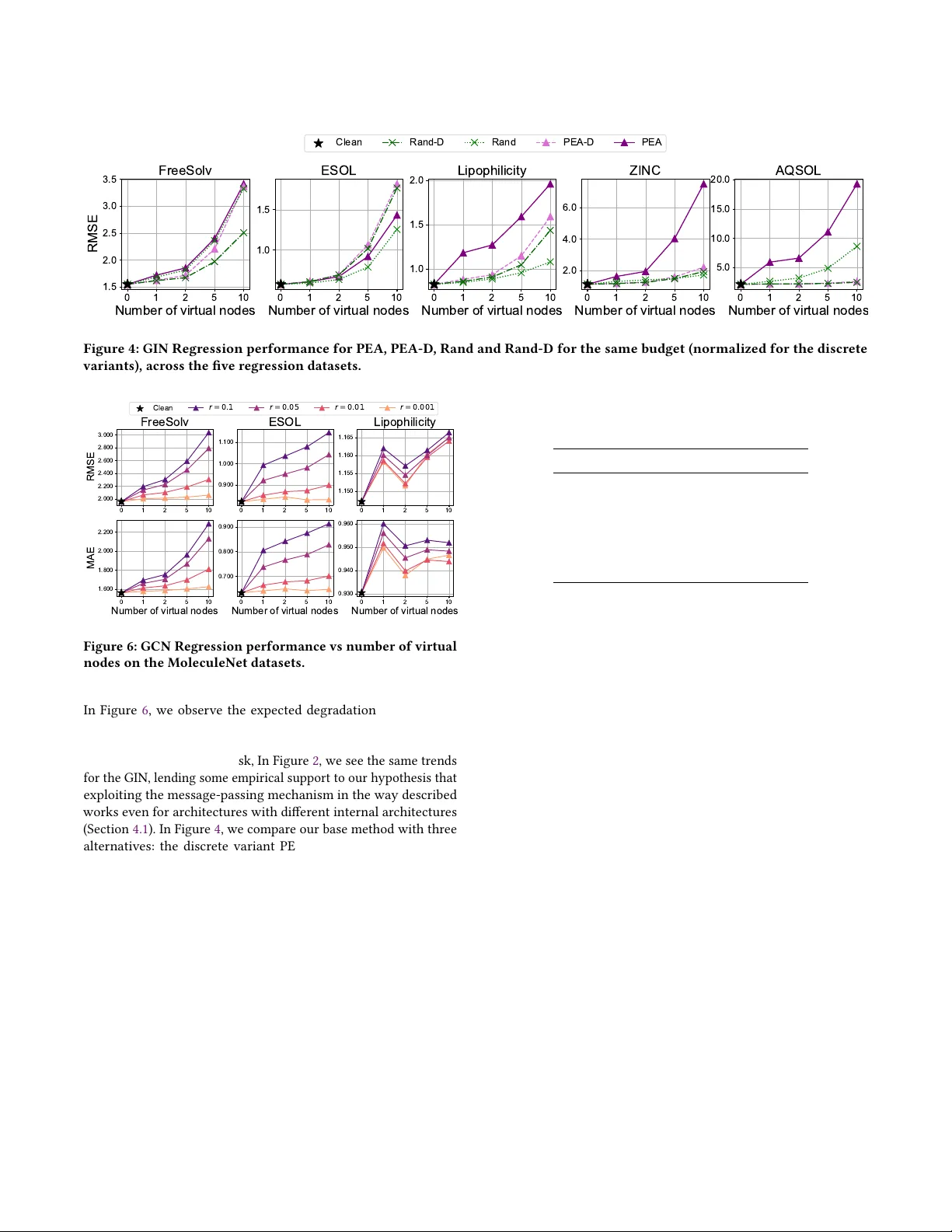
PEAN U T: Perturbations by Eigenvector Alignment for Aacking Graph Neural Networks Under T opology-Driven Message Passing Bhavya Kohli ∗ College of Design and Engineering National University of Singapore Singapore bhavyakohli@u.nus.edu Biplap Sikdar College of Design and Engineering National University of Singapore Singapore bsikdar@nus.edu.sg Abstract Graph Neural Networks (GNNs) have achiev ed remarkable perfor- mance on tasks involving relational data. How ever , small pertur- bations to the graph structure can signicantly alter GNN outputs, raising concerns about their robustness in real-world deployments. In this work, we explor e the core vulnerability of GNNs which explicitly consume graph topology in the form of the adjacency matrix or Laplacian as a means for message passing, and pr opose PEANU T , a simple, gradient-free, restricted black-box attack that injects virtual nodes to capitalize on this vulnerability . PEAN U T is a injection based attack, which is widely considered to be more prac- tical and realistic scenario than graph modication attacks, where the attacker is able to modify the original graph structure directly . Our method works at the inference phase, making it an evasion at- tack, and is applicable almost immediately , since it does not inv olve lengthy iterative optimizations or parameter learning, which add computational and time overhead, or training surrogate mo dels, which are susceptible to failure due to dier ences in model priors and generalization capabilities. PEAN UT also does not require any features on the injected node and consequently demonstrates that GNN performance can be signicantly deteriorated even with in- jected no des with zeros for features, highlighting the signicance of eectively designed connectivity in such attacks. Extensive experi- ments on real-world datasets across three graph tasks demonstrate the eectiveness of our attack despite its simplicity . CCS Concepts • Security and privacy → Software and application security ; • Theory of computation → Machine learning theor y ; • Math- ematics of computing → Graph algorithms . Ke ywords Graph Neural Networks; Graph Injection Attacks; Black-box A d- versarial Attacks; Adv ersarial Robustness; Graph-level Learning 1 Introduction Graph Neural Networks (GNNs) have emerged as a central model- ing paradigm for learning over relational and structured data across a wide range of applications including molecular property predic- tion [ 8 , 26 ], physical simulation [ 19 ], trac forecasting [ 11 , 16 ], recommendation systems [ 30 ], and knowledge graph reasoning [ 20 ]. They are increasingly deployed in high-impact settings where adver- sarial robustness is a practical concern. Their success largely stems ∗ Corresponding Author: Bhavya K ohli This work is a preprint from message passing, where node repr esentations are iteratively updated by aggregating information from local neighborho ods. Howev er , this same mechanism also exposes GNNs to structural vulnerabilities: small, carefully crafted changes in the graph can propagate through the network and lead to signicant p erformance degradation. Early studies on adversarial attacks against GNNs primarily fo- cus on graph-modication attacks, where the adversar y perturbs existing edges or node features [ 5 , 34 , 35 ]. While eective in con- trolled settings, these attacks often rely on unrealistic assumptions about the attacker’s capability such as having direct access to an existing graph’s topology and being able to mo dify its attributes. In many real-world systems ( e.g., social networks, citation graphs, recommendation systems), modifying existing users, items, or rela- tionships is generally infeasible . In contrast, graph injection attacks provide a mor e practical threat model where the adversar y intr o- duces new nodes into the graph and conne cts them to existing nodes without altering the original graph structure [ 13 , 22 , 24 , 32 ]. Such at- tacks reect more realistic scenarios, such as creating fake accounts or synthetic entities to inuence downstream performance. Evasion and poisoning attacks. Depending on the target phase (i.e., training or inference), adversarial attacks on GNNs may b e cate- gorized into two settings, i.e., poisoning and evasion. In poisoning attacks, the adversary injects malicious nodes into the training graph so that the model is trained on corrupted data and exhibits degraded performance at inference [ 22 , 24 , 33 ]. In evasion attacks, the GNN is assumed to be already trained, and the attacker injects new nodes at test time to manipulate predictions without retraining the mo del [ 5 , 13 , 32 ]. This paper fo cuses on the evasion setting, which is particularly relevant for deployed GNN systems where retraining is costly or infrequent, and wher e adversaries can only interact with the system by introducing new entities at inference. Vulnerability of adjacency-input architectures. Many widely used GNN architectures explicitly utilize the adjacency (or Laplacian) matrix [ 7 , 15 , 25 ] as message-passing operators. This design choice introduces a major architectural vulnerability: perturbations to the adjacency matrix directly alter the propagation pathways through which information ows, aecting the graph’s receptive elds, ag- gregation neighborhoods, and sp ectral properties. This ultimately results in amplied, nonlocal changes in downstr eam representa- tion. Unlike feature perturbations, which are often normalized or regularized, such adjacency perturbations modify the structure of the computation graph itself. Despite recent progress on graph injection attacks, most existing methods remain limited in both practicality and scope. A large Bhavya Kohli and Biplap Sikdar fraction of prior work relies on per-graph iterative optimization or reinforcement learning to construct the injected nodes’ features and edges, which is computationally expensive and must be repeate d for every target graph or attack instance [ 17 , 22 – 24 ]. Moreover , current injection attacks are predominantly evaluated on node-level tasks such as node classication, with limited evidence of eectiveness beyond this narrow setting [ 13 , 22 , 23 ]. Several recent approaches approximate the victim GNN by training surrogate models, which may b e insucient to having dierent priors and generalization capabilities, while also introducing additional time and resource overhead for their training. This makes the attack pip eline even more cumbersome in practice, and limits its applicability in large- scale or real-time settings. Contributions. T o address the aforementioned drawbacks of pre vi- ous works, we propose a black-box attack, namely P erturbation by E igenvector A lignment for Graph Neural N etworks U nder T opology- driven message passing ( PEANU T ), which works on the evasion set- ting. Our proposed method can be applied immediately to a trained GNN without any per-graph optimization or surrogate model train- ing, only r equires the attacker to view the nal no de-lev el r epresen- tations. Furthermore, it generalizes beyond node classication and can be directly applied to GNNs trained for arbitrary graph-level objectives, including the largely undere xplored graph regression setting. W e summarize our contributions as follows: • W e identify a restricted black-box attack surface induced by GNN architectures that explicitly utilize graph topology matrices for message passing. • W e propose a simple, gradient and surrogate-free , restricted black-box attack that injects virtual nodes to maximize dier- ences between clean and perturbe d graph repr esentations. • W e provide the rst known systematic evaluation of such attacks on graph-level r egression tasks, demonstrating that even small perturbations can meaningfully degrade perfor- mance on graph regression benchmarks. 1.1 Threat Model W e consider a restricted black-box threat model which works at the inference phase (evasion attack). The attacker has no access to model parameters, gradients, or training data, but can observe only the nal node-level r epresentations during inference (e.g. output logits or log-probabilities for a node classier , node representations prior to graph-pooling operations for graph-level tasks). This set- ting reects modular deployment pip elines in which node-level embeddings are utilize d by downstream components, while the un- derlying components themselves remain black boxes. The attacker is allowed to perturb the input graph structure via virtual node injection, subject to a perturbation budget. The goal of the attacker is to induce large deviations in the generated embeddings by con- structing perturbed graphs that maximize a discrepancy measure between clean and attacked graph representations. 2 Related works Structural Attacks on GNNs. Adversarial attacks on graph neural networks (GNNs) frequently target the graph structure by mod- ifying the adjacency matrix through edge additions or deletions. Early white-box methods assume full access to model parameters and gradients, e.g. Nettack [ 33 ] performs targeted perturbations of edges and features to induce misclassications under structural constraints. Meta-learning-based poisoning attacks optimize the adjacency in a bi-level formulation to maximally degrade down- stream performance [ 35 ]. Gradient-based topology attacks, such as Fast Gradient Attack (FGA) [ 2 ], relax discrete e dges into con- tinuous variables and greedily select perturbations via gradients. These approaches demonstrate that small structural changes can signicantly impact GNN predictions, but r ely on strong white-b ox assumptions, and work on the graph modication that are unrealis- tic in many deployment settings. On the other hand, black-box, or restricted black-box approaches such as GF- Attack [ 1 ], work under more feasible attack assumptions where attackers do not observe model parameters, gradients, or training data, but may assume access to restricted internal repr esentations or condence scores. Alternative black-box settings with no model queries have also been explored by optimizing surrogate spe ctral objectives that aim to maximally alter the implicit graph lters induced by GNNs [ 27 ]. A few more classical white-box and recent black-box methods are summarized in [ 3 , 12 , 21 ]. Graph Inje ction Attacks. A growing body of work studies graph injection attacks, where adversaries introduce malicious nodes to degrade GNN performance without mo difying existing graph struc- ture. The Node Injection Poisoning Attack (NIP A) [ 22 ] injects no des during training using deep reinforcement learning to sequentially optimize edges and labels under a white-b ox setting. Due to its high compute requirements, it is considered not scalable for large-scale datasets [ 32 ]. Under the black-box setting, T opological Defective Graph Injection Attack (TDGIA) [ 32 ] oers a scalable inference- time inje ction attack that relies on iterativ e optimization of injecte d node features and connectivity , howe ver it relies on training surro- gate models for its attack mechanism. T o maintain the unnotice- ability of inje ction attacks, Chen et al . [ 4 ] propose A GIA, a dieren- tiable realization of the graph homophily constraint, showing that constraining injected no des to match lo cal homophily improves unnoticeability while maintaining their respective attack success. An extremely limited scenario of a single-node injection attack is considered in T ao et al . [ 23 ] , wherein the objective is to nd the most damaging injected node by a carefully crafted optimization scheme. This is further extended as the Generalizable Node Injec- tion Attack model (G-NIA) which can work in black-box settings to amortize the per-graph optimization cost, although requiring a generator model to b e trained. The Gradient-free Graph A dvantage Actor Critic mo del (G2A2C) [ 13 ] uses reinforcement learning to discover injection policies through r epeated interaction with the target model, incurring substantial quer y and training overhead in the process. QUGIA [ 17 ], a Query-based and Unnoticeable Graph Injection Attack, tries to avoid the need to train surrogate models, howev er it still requires iterative sampling and distribution updates per target graph. Zhou et al . [ 31 ] extend graph inje ction attacks to graph-level classication under a hard-label black-box setting, building upon existing edge perturbing attacks, using quer y-based optimization to inject nodes that ip graph predictions. Graph-level tasks and regression. Most prior work on structural at- tacks focus on node classication, with some exploring the eects PEANU T: Perturbations by Eigenvector Alignment for Aacking GNNs Under T op ology-Driven Message Passing Weighted edges (discarded) Attacker Operations Virtual node Figure 1: PEA when use d on a graph-level task. The attacker queries the model once to obtain the (clean) no de-lev el embeddings, using them to create the p erturbation S 𝑣 using the eigenvector u 1 of ZZ ⊤ which induces a high L ( S 𝑣 ) . on graph-level classication. Graph-level r egression tasks, such as molecular pr operty prediction or physical system modeling, remain comparatively underexplor ed in adversarial literature. In contrast to prior black-box approaches that rely on learning-based policies or query-driven optimization, our method leverages nal node-level representations to construct gradient-free structural perturbations. W e demonstrate that maximizing the norm discr epancy between clean and perturbed graphs constitutes an ee ctive attack objec- tive for graph-level r egression, rev ealing a previously unexplor ed vulnerability of architectures that explicitly utilize graph topology matrices, such as the adjacency matrix or graph Laplacian, as input. Furthermore, we demonstrate that this sort of norm discrepancy also translates to drops in performance in classication-based tasks. 3 Preliminaries Let G ( V , A , X ) be an undirected attributed graph with vertex set V of size 𝑁 , and adjacency matrix A ∈ R 𝑁 × 𝑁 with associated edge set E . W e denote the node attributes of G as X ∈ R 𝑁 × 𝐷 , and following the notation in Wu et al . [ 25 ] , we denote the normalized adjacency matrix as S = D − 1 / 2 AD − 1 / 2 , where D is the diagonal degree matrix of A , and D 𝑖𝑖 = Í 𝑗 A 𝑖 𝑗 . W e consider a graph neural network (GNN) with parameters 𝚯 , denote d M 𝚯 ( A , X ) , which uses the graph adjacency matrix and node attributes as inputs to produce task-specic outputs. For node-level tasks, such as node classication with C classes, the network M 𝚯 outputs log-probabilities (or unnormalized logits) Z ∈ R 𝑁 × C . For graph-lev el tasks, we represent the model as a composition M 𝚯 ( 𝐴, 𝑋 ) = M 𝑜𝑢 𝑡 𝚯 1 ( P ool ( M 𝑎𝑔 𝑔 𝚯 2 ( 𝐴, 𝑋 ) ) ) , (1) where M 𝑎𝑔 𝑔 𝚯 2 rst computes node-level embeddings Z ∈ R 𝑁 × 𝑑 which are then poole d to produce a single graph-level represen- tation. This po oled embedding is nally reduced by the readout network M 𝑜𝑢 𝑡 𝚯 1 to either a vector of C values (graph-lev el classica- tion with C classes), or a single value (graph-lev el regression). This follows the design ow commonly used in molecular and physical system applications [ 8 , 26 ]. Virtual-node perturbation. For a graph G , we dene a virtual-node perturbation as the adjacency matrix with 𝑛 𝑣 injected virtual no des with the real-virtual, virtual-real, and virtual-virtual node connec- tions dened by matrices A 𝑟 , 𝑣 , A 𝑣,𝑟 , and A 𝑣,𝑣 respectively . The adja- cency matrix of the perturbed graph with 𝑁 𝑝 = 𝑁 + 𝑛 𝑣 nodes is de- ned as A 𝑝 ∈ R 𝑁 𝑝 × 𝑁 𝑝 . T o minimize the number of new edges added, we consider A 𝑣,𝑣 = 0 𝑛 𝑣 × 𝑛 𝑣 , and to maintain symmetr y , we consider A 𝑟 , 𝑣 = A ⊤ 𝑣,𝑟 = A 𝑣 ∈ R 𝑁 × 𝑛 𝑣 . Thus, a perturbation is uniquely deter- mined by A 𝑣 . If we work with the normalized adjacency matrix S , the perturbe d matrix follows the same structure, with S 𝑣 instead of A 𝑣 . The perturbed matrix is thus dene d as: A 𝑝 =  A A 𝑣 A ⊤ 𝑣 0  . (2) Bhavya Kohli and Biplap Sikdar The feature matrix of the perturbed graph is denoted by X 𝑝 =  X ˜ X  ⊤ ∈ R 𝑁 𝑝 × 𝐷 . T o simplify the closed-form expression in Theorem 1 , we assign a vector of zeros to all virtual nodes. W e refer to the perturbed graph as G 𝑝 . Simplied Graph Convolution Network (SGC). The simplied linear version of a Graph Convolution Network (GCN) [ 15 ], has been shown to perform similarly , if not better , than GCNs at tasks such as node classication and text classication [ 25 ]. Given a 2-Lay er SGC , we denote Z as the node embeddings for an unperturbe d graph, i.e., Z = S 2 X 𝚯 . Additionally , we dene the node embeddings for the real nodes of a perturbed graph as Z 𝑝 , which is S 2 𝑝 X 𝑝 𝚯 [ : 𝑁 , : ] , i.e., the rst 𝑁 rows of S 2 𝑝 X 𝑝 𝚯 . Attack Ecacy and Constraints. W e dene the attack ecacy (de- noted by L ( S 𝑣 ) ) of perturbation S 𝑣 as the norm of the dierence of node embeddings of the real nodes for the original and perturbed graphs, i.e., L ( S 𝑣 ) =   Z 𝑝 − Z   2 𝐹 . T o constrain the perturbation which maximizes L , we impose a norm constraint   S 𝑣 S ⊤ 𝑣   𝐹 ≤ 𝚫 . If the perturbation S 𝑣 were binary , this would correspond to a b ound on the exact number of new edges being added. Our main optimiza- tion objective, therefore , is as follows: max S 𝑣 ∈ R 𝑁 × 𝑛 𝑣 L ( S 𝑣 ) =   Z 𝑝 − Z   2 𝐹 s . t .   S 𝑣 S ⊤ 𝑣   𝐹 ≤ 𝚫 . (3) For a Simple Graph Convolution network, L ( S 𝑣 ) reduces to the following, assuming ˜ X = 0 (See Appendix A.1 ): L ( S 𝑣 ) =   Z 𝑝 − Z   2 𝐹 =   S 𝑣 S ⊤ 𝑣 X 𝚯   2 𝐹 . (4) 3.1 Attack Goal For the class of GNNs dened above, admitting the adjacency ma- trix A (or S , or graph Laplacian L , etc.) as the input introduces a structural vulnerability . Our proposed attack injects virtual no des with carefully chosen e dge weights, aiming to mo dify the node- level emb eddings Z and thereby degrading performance on the downstream task. The attack is gradient-free and requires no access to model parameters 𝚯 . For node-level tasks, this makes the at- tack strictly black-box; for graph-level tasks, it relies on observing the intermediate output of M 𝑎𝑔 𝑔 𝚯 2 , making it a r estricted black-box method overall. As shown in Section 5.2 , this approach is eective across a variety of commonly used architectures, demonstrating that even limited adjacency p erturbations can induce substantial changes in graph-level outputs. 4 Methodology In this section, we dene the base version of our method, which, for brevity , we will refer to as PEA , for P erturbation by E igenvector A lignment . First, we dene a white-box variant for the SGC ar- chitecture in Theorem 1 which requires knowledge of the model parameters 𝚯 . W e refer to this variant as PEA - W . Then, in Section 4.1 , we propose the black-box formulation, which also signicantly deteriorates GNN performance. W e follo w this with a discussion on the practical considerations of generating perturbations in this manner , and comment on the dierences in how w e should inter- pret the results for three dierent graph-based tasks. The ow of PEA is summarized in Figure 1 , and in Algorithms 1 - 2 in Appendix B . Before proving the result in Theorem 1 , we rst need a key result: Lemma 1. For a given real-valued Z ∈ R 𝑁 × 𝑑 , and budget 𝚫 , we dene the following optimization obje ctive: max B ∈ R 𝑁 × 𝑛   BB ⊤ Z   2 𝐹 s . t .   BB ⊤   𝐹 ≤ 𝚫 . (5) The solution B ∗ for the above is B ∗ = 𝚫 · u 1 v ⊤ , where u is the dominant eigenvector (corresponding to the eigenvalue of largest magnitude) of ZZ ⊤ , and v is any unit-norm vector in R 𝑛 . Proof. The proof uses the trace-equivalent representation of the frobenius norm, followed by the eigen-decomposition of ZZ ⊤ . See Appendix A for more details. □ Theorem 1. Given a trained 2-Layer Simple Graph Convolution network M Θ , and graph G ( V , A , X ) , the p erturbation S 𝑣 which max- imizes L ( S 𝑣 ) while satisfying   S 𝑣 S ⊤ 𝑣   𝐹 ≤ 𝚫 , is given by S ∗ 𝑣 = 𝚫 · u 1 v , (6) where u 1 is the dominant eigenvector of H H ⊤ ( H = X 𝚯 ), and v is any vector with unit norm. Proof. Using the formulation of L ( S 𝑣 ) dened for the SGC in Equation 4 , we can apply Lemma 1 to obtain S ∗ 𝑣 . □ W orking with Limited Information. With this simple result, assum- ing there are no limitations, we can obtain a budget-constrained perturbation S 𝑣 which induces the maximum change in the output Z = M Θ ( A , X ) . W e can, however , make this work in a black-box manner by using Z instead of H . Considering the Cauchy-Schwarz inequality and the formulation in Equation 4 ,   S 𝑣 S ⊤ 𝑣 𝑍   2 𝐹 =   S 𝑣 S ⊤ 𝑣 ( S 2 X 𝚯 )   2 𝐹 (7) ≤   S 2   2 𝐹   S 𝑣 S ⊤ 𝑣   2 𝐹 ∥ X 𝚯 ∥ 2 𝐹 (8) =   S 2   2 𝐹 ·  𝚫 2 ∥ H ∥ 2 𝐹  (9) =   S 2   2 𝐹 ·   S 𝑣 S ⊤ 𝑣 X 𝚯   2 𝐹 (10) Thus, if we assume the attacker only has access to the outputs Z , maximizing the LHS using Lemma 1 would also push up the RHS, albeit at a lesser eect (see Figure 5 ). Choice of v . For the SGC , the choice of v has no eect on the out- puts since it gets reduced to 1 when computing S 𝑣 S ⊤ 𝑣 . This will not happen in more complex GNN architectures, which may have possible activations or biases inside it, making it a point of further optimization. T o keep things simple, howev er , we only adopt two main methods to obtain v : (1) Sampling v ∈ R 𝑛 𝑣 from the standard uniform distribution; and (2) Setting v = 1 𝑛 𝑣 , i.e., a vector of ones. Both are followed by normalization to unit norm. PEANU T: Perturbations by Eigenvector Alignment for Aacking GNNs Under T op ology-Driven Message Passing Statistic \ Dataset FreeSolv ESOL Lipophilicity ZINC A QSOL MU T AG PROTEINS ENZYMES IMDB-BINARY BBBP BACE Number of Graphs 641 1126 4200 12000 9833 188 1113 600 1000 2039 1513 Number of Classes - - - - - 2 2 6 2 2 2 A vg. Number of No des 8.73 13.29 27.04 23.16 17.58 17.93 39.06 32.63 19.77 24.06 34.09 A vg. Number of Edges 25.51 40.63 86.04 72.99 53.38 57.52 184.69 156.91 212.84 75.97 107.81 A vg. Degree 2.83 2.98 3.18 3.14 2.98 3.19 4.73 4.86 9.89 3.13 3.17 A vg. 𝚫 for 𝑟 = 0 . 05 1.28 2.03 4.30 3.65 2.67 2.88 9.23 7.85 10.64 3.80 5.39 T able 1: Dataset summar y for the GR and GC tasks. Norm Dierences and its Eectiveness in Classication Tasks. PEA provides a way to augment the graph topology matrix being consid- ered in order to maximize the norm of the dierence of node-level representations of a graph. The way PEA performs this do es not have any control on where all the norm dierence goes; for the node classication task, if the eect of perturbation on Z happen to somehow maintain the relative ranking or der , the attack will have no eect on the actual predicted classes at test time. W e will see in Section 5.2.1 , however , that PEA does display its eectiveness despite this theoretical pitfall. W e observe the same for the graph classication task, maximizing norm dierence before the read- out model M 𝑜𝑢 𝑡 𝚯 1 causes enough perturbation to cause signicant misclassications (Section 5.2.3 ). Compared to the classication datasets, the graph regression task is much more sensitiv e to such an induced norm change. A pplicability to other GNNs. Consider a 2-lay er GIN mo del with the internal MLP being a Linear-ReLU-Linear (LRL) model with no bias. The forward-direction update would be as follows: H ( 1 ) = MLP ( 1 )   ( 1 + 𝜀 ( 1 ) ) · I + A  X  , (11) Z = MLP ( 2 )   ( 1 + 𝜀 ( 2 ) ) · I + A  H ( 1 )  . (12) It has been observed [ 28 ] that when the parameters 𝜀 ( 1 ) , 𝜀 ( 2 ) are set to zero, the resulting GIN (denoted GIN -0) consistently outperforms GIN with nonzero, and ev en trainable 𝜀 , in terms of test accuracy . W riting this in the form of weights W 1 − 4 for the two MLP ’s, and denoting ˆ A = I + A Z = 𝜎  ˆ AH ( 1 ) W 3  W 4 , (13) Z = 𝜎  ˆ A  𝜎 ( ˆ AXW 1 ) W 2  W 3  W 4 . (14) Under a naïve assumption of r emoving nonlinearities, this shows the exact same form as SGC . W e do not actually use this version of GIN since it is essentially the same model as SGC and does not per- form as well on graph-level tasks, howev er , we want to note that the pathway for message passing remains some what similar . While our theoretical results are established for a specic architecture type, we hypothesize that exploiting the message-passing mechanism in the same way remains eective even if the specic model incorpo- rates internally complex message passing mechanisms compared to the SGC, and validate this empirically in Section 5.2 . 4.1 Practical Considerations 4.1.1 Perturbations With Negative Edge W eights. In the above, we do not constrain positivity on the generated perturbation S 𝑣 , and using eigenvector u 1 means that there is no contr ol over whether the p erturbation will be p ositive or not. In principle, if a GNN simply admits an adjacency matrix as input with no restrictions or checks on whether edge weights ar e non-negative, this would not be an issue. Howe ver , considering that these perturbations may be simply “defended" by using one ReLU call on the adjacency matrix before the propagation steps, we assume as such, and tr y to minimize the number of perturbation connections which are zeroed out. This makes the generated perturbations positive with values ∈ [ 0 , 1 ] . T o this end, we rst switch the direction of u 1 to have the maximum numb er of p ositive terms as follows: u 1 is assigne d a sign based on the numb er of positive and negative elements in it, using u 1 = u 1 · sign ( Í sign ( u 1 ) ) . With this operation, the eigenvalue ordering remains unaected as the magnitude is unchanged. The method of obtaining v dene d above ensur es that the number of surviving elements does not experience further change after the 𝚫 · u 1 v ⊤ product. W e refer to this as the base metho d ( PEA ), and refer to the unconstrained version where models simply admit an adjacency matrix without imposing positivity as PEA-U. 4.1.2 A rchitectures Which Admit Only Binary Adjacency . In case the GNN does not explicitly utilize edge weights ( GIN , SA GE , etc.,) and essentially processes the adjacency matrix as if it were binary , we discretize the generate d perturbation A 𝑣 by picking the top- k entries for each virtual node where 𝑘 = max ( round ( 𝚫 / 𝑛 𝑣 ) , 1 ) . Since we have lesser means to distribute the available budget in this discrete case, we assign at least one edge for each virtual no de, making the minimum possible perturbation equal to 2 𝑛 𝑣 ( 𝑛 𝑣 each for S 𝑣 and S ⊤ 𝑣 ). This is usually only relevant on graph datasets with smaller graphs, where a low 𝑟 = 0 . 01 may correspond to a value less than 1 . The eective budget 𝚫 ′ in this case is essentially 𝑛 𝑣 𝚫 . W e refer to this version of PEA as PEA-D 5 Experiments In this section, we empirically evaluate PEANU T on three graph tasks—Node Classication (NC), Graph Classication (GC), and Graph Regression (GR). 5.1 Experimental Setup 5.1.1 Datasets. W e evaluate the ecacy of PEA on NC using the three benchmark citation networks—Cora, Citeseer , and Pubmed [ 29 ], and compare its performance with baselines. Then, we eval- uate PEA on ve benchmark regression datasets—ESOL, Fr eeSolv , and Lipophilicity [ 26 ], ZINC [ 9 ], and A QSOL [ 6 ], and on GC us- ing four benchmark graph classication datasets from T UDataset [ 18 ]—MU T AG, PROTEINS, ENZYMES, and IMDB-BINARY , and two datasets from MoleculeNet [ 26 ]—BBBP and BACE, for a total of six datasets spanning molecular property prediction, social networks, Bhavya Kohli and Biplap Sikdar                                                                                                                          r = 0 . 1 r = 0 . 0 5 r = 0 . 0 1 r = 0 . 0 0 1 Figure 2: GIN Regression performance vs numb er of virtual nodes on the ve regression datasets. Dataset 𝑟 𝑛 𝑣 Clean Graph A GIA TDGIA A TDGIA PEA (Ours) Accuracy F1 Score Accuracy ↓ F1 ↓ Accuracy ↓ F1 ↓ Accuracy ↓ F1 ↓ Accuracy ↓ F1 ↓ Cora 0.001 2 78 . 48 ± 2 . 53 72 . 77 ± 4 . 92 0 . 04 ± 0 . 11 0 . 03 ± 0 . 08 0 . 07 ± 0 . 15 0 . 05 ± 0 . 10 0 . 07 ± 0 . 15 0 . 07 ± 0 . 15 0 . 07 ± 0 . 17 0 . 04 ± 0 . 17 0.01 27 2 . 52 ± 0 . 62 2 . 21 ± 0 . 62 2 . 41 ± 0 . 48 2 . 04 ± 0 . 56 3 . 78 ± 0 . 92 5 . 11 ± 1 . 69 0 . 72 ± 0 . 42 0 . 57 ± 0 . 42 0.05 135 8 . 96 ± 1 . 18 10 . 24 ± 1 . 58 9 . 81 ± 1 . 55 11 . 05 ± 1 . 89 12 . 78 ± 2 . 25 13 . 55 ± 2 . 24 36 . 12 ± 1 . 94 45 . 34 ± 3 . 18 0.1 270 12 . 44 ± 1 . 30 13 . 38 ± 1 . 69 13 . 00 ± 1 . 45 13 . 72 ± 1 . 88 14 . 52 ± 2 . 00 15 . 05 ± 2 . 35 51 . 65 ± 0 . 77 73 . 08 ± 0 . 77 Citeseer 0.001 3 77 . 68 ± 0 . 89 67 . 38 ± 1 . 33 0 . 15 ± 0 . 15 0 . 11 ± 0 . 11 0 . 15 ± 0 . 15 0 . 11 ± 0 . 11 0 . 18 ± 0 . 15 0 . 17 ± 0 . 13 0 . 00 ± 0 . 07 − 0 . 00 ± 0 . 06 0.01 33 2 . 26 ± 0 . 28 2 . 03 ± 0 . 24 2 . 32 ± 0 . 52 2 . 08 ± 0 . 48 1 . 99 ± 0 . 63 1 . 92 ± 0 . 58 0 . 26 ± 0 . 52 0 . 45 ± 0 . 70 0.05 166 8 . 61 ± 0 . 45 7 . 68 ± 0 . 44 8 . 49 ± 0 . 87 7 . 58 ± 0 . 73 12 . 92 ± 0 . 68 11 . 23 ± 0 . 59 15 . 16 ± 6 . 65 17 . 97 ± 6 . 46 0.1 332 11 . 05 ± 0 . 82 9 . 66 ± 0 . 74 10 . 81 ± 0 . 61 9 . 55 ± 0 . 57 14 . 61 ± 1 . 44 12 . 62 ± 1 . 22 37 . 64 ± 7 . 82 45 . 38 ± 8 . 29 Pubmed 0.001 19 85 . 80 ± 0 . 24 84 . 71 ± 0 . 24 0 . 04 ± 0 . 02 0 . 03 ± 0 . 03 0 . 02 ± 0 . 02 0 . 03 ± 0 . 03 0 . 03 ± 0 . 09 0 . 02 ± 0 . 11 0 . 21 ± 0 . 14 0 . 33 ± 0 . 17 0.01 197 0 . 76 ± 0 . 26 0 . 76 ± 0 . 26 0 . 72 ± 0 . 26 0 . 72 ± 0 . 31 1 . 10 ± 0 . 10 1 . 16 ± 0 . 15 4 . 33 ± 0 . 76 7 . 24 ± 1 . 48 0.05 985 3 . 99 ± 0 . 37 4 . 14 ± 0 . 41 3 . 78 ± 0 . 51 3 . 88 ± 0 . 51 10 . 22 ± 1 . 08 10 . 65 ± 1 . 11 34 . 24 ± 4 . 64 50 . 24 ± 5 . 42 0.1 1971 11 . 98 ± 1 . 14 12 . 39 ± 1 . 30 11 . 54 ± 0 . 97 11 . 88 ± 1 . 19 11 . 98 ± 1 . 13 12 . 29 ± 1 . 31 41 . 78 ± 1 . 56 61 . 09 ± 2 . 35 T able 2: Results of PEA and the baselines on Node classication using the GCN architecture as the defending model. The accuracy and (macro) F1 score on the clean datasets are reported rst, followed by their respective decrease for each method. biophysics and physiology . W e summarize some key statistics of these datasets in T ables 3 and 1 . Statistic \ Dataset Cora Citeseer Pubmed Number of Classes 7 6 3 Number of Nodes 2708 3327 19717 Number of Edges 10556 9104 88648 A vg. Degree 4.90 3.74 5.50 𝑛 𝑣 for 𝑟 = 0 . 01 27 33 197 𝚫 for 𝑟 = 0 . 01 132 124 1083 T able 3: Dataset summar y for the NC task. 5.1.2 Metrics. For the regr ession datasets, w e report the test RMSE and MAE; and for the classication datasets, we compute the accu- racy and macro-averaged F1 scor e (denoted by F1) on the test set, both as percents. Unless other wise mentioned, all reported numb ers have been averaged over 10 runs. 5.1.3 Aack Budgets. For NC, we follow the budget allowances as in Sun et al . [ 22 ] , ke eping the number of virtual no des 𝑛 𝑣 = 𝑟 · | 𝑉 | and 𝚫 = 𝑟 · | 𝑉 | · deg ( G ) , where deg ( G ) is the average degree of the graph. For GC and GR, we consider the budget 𝚫 available to the attacker as a fraction 𝑟 of the number of e dges of each individual graph, i.e., 𝚫 = 𝑟 · | E ( 𝑖 ) | for graph G ( 𝑖 ) , and we vary 𝑛 𝑣 ∈ [ 0 , 1 , 2 , 5 , 10 ] . 5.1.4 Baselines. Since node injection attacks remain underexplor ed on the GC and GR tasks, we compare the performance of PEA with baselines on the well-studied and benchmarked NC task. W e use TDGIA [ 32 ], A TDGIA, a variant of TDGIA proposed by [ 4 ], and A GIA [ 4 ] as three key baselines. TDGIA involves topological de- fective edge selection followed by featur e learning using smooth adversarial optimization. A GIA requires gradient information ( via the surrogate) to learn the features and structures of the injected nodes. For a fair comparison, we impose our attack budget con- straints dened in Section 5.1.3 for deciding the number of injected nodes and the corresponding perturbation budget. 5.1.5 A rchitectures. For NC, we use the SGC [ 25 ], GCN [ 15 ], GIN [ 28 ], and SA GE [ 10 ] architectures for evaluating the eects of PEA - style perturbations across models with dierent propagation styles. PEANU T: Perturbations by Eigenvector Alignment for Aacking GNNs Under T op ology-Driven Message Passing                                                                                                          r = 0 . 1 r = 0 . 0 7 5 r = 0 . 0 2 5 r = 0 . 0 1 Figure 3: GIN Classication accuracy vs number of virtual no des on the six classication datasets. All reported numbers have been averaged over the 10-Fold CV . The GIN , and SA GE architectures usually do not admit the adja- cency matrix as-is since they only deal with unattributed aggrega- tion over neighbors. However common implementations often use products of the form AX as a parallelizable and ecient aggregation step, which is an e xploitable vulnerability for PEA . The architecture of choice for graph-level tasks will be a 2-layer GIN. Ho wever , for a few simple graph-regression datasets, we also train a GCN to conrm our performance trends. For all tasks, each architecture described consists of 2 graph convolution layers of the spe cied architecture. 5.2 Results Dataset Model 𝑟 𝑛 𝑣 Accuracy (F1) Accuracy ↓ ( F1 ↓ ) Cora SGC 0.05 135 83 . 77 ( 82 . 42 ) 35 . 97 ( 45 . 52 ) 0.1 270 83 . 77 ( 82 . 42 ) 52 . 03 ( 73 . 76 ) GCN 0.05 135 83 . 33 ( 81 . 71 ) 38 . 28 ( 49 . 63 ) 0.1 270 83 . 33 ( 81 . 71 ) 51 . 70 ( 73 . 37 ) GIN 0.05 135 79 . 30 ( 76 . 63 ) 44 . 44 ( 64 . 49 ) 0.1 270 79 . 30 ( 76 . 63 ) 47 . 97 ( 68 . 12 ) SA GE 0.05 135 84 . 01 ( 82 . 56 ) 5 . 71 ( 5 . 94 ) 0.1 270 84 . 01 ( 82 . 56 ) 10 . 61 ( 11 . 36 ) Citeseer SGC 0.05 166 75 . 32 ( 71 . 53 ) 7 . 50 ( 10 . 09 ) 0.1 332 75 . 32 ( 71 . 53 ) 31 . 40 ( 36 . 49 ) GCN 0.05 166 74 . 86 ( 71 . 12 ) 13 . 83 ( 16 . 98 ) 0.1 332 74 . 86 ( 71 . 12 ) 36 . 45 ( 43 . 75 ) GIN 0.05 166 68 . 11 ( 64 . 27 ) 50 . 18 ( 57 . 43 ) 0.1 332 68 . 11 ( 64 . 27 ) 45 . 29 ( 51 . 89 ) SA GE 0.05 166 74 . 86 ( 70 . 73 ) 1 . 65 ( 2 . 34 ) 0.1 332 74 . 86 ( 70 . 73 ) 3 . 22 ( 4 . 33 ) Pubmed SGC 0.05 985 83 . 09 ( 82 . 40 ) 35 . 10 ( 50 . 94 ) 0.1 1971 83 . 09 ( 82 . 40 ) 41 . 54 ( 60 . 94 ) GCN 0.05 985 83 . 63 ( 82 . 96 ) 36 . 15 ( 52 . 43 ) 0.1 1971 83 . 63 ( 82 . 96 ) 42 . 25 ( 61 . 84 ) GIN 0.05 985 75 . 84 ( 67 . 66 ) 35 . 84 ( 46 . 54 ) 0.1 1971 75 . 84 ( 67 . 66 ) 37 . 09 ( 48 . 37 ) SA GE 0.05 985 85 . 27 ( 84 . 99 ) 1 . 94 ( 2 . 22 ) 0.1 1971 85 . 27 ( 84 . 99 ) 3 . 43 ( 4 . 08 ) T able 4: Performance of PEA on NC across GNN architectures. 5.2.1 No de Classification. In T able 2 ., we compare the performance of PEA with the current state-of-the art baselines. Despite not being designed explicitly for node classication, and with the pitfalls discussed in Section 4 when dealing with classication-based tasks, PEA performs well across the board, and signicantly outperforms the baselines on slightly higher budgets ( ∼ 5% inje cted nodes). Note that the GCN architecture here is assumed to be one which normalizes the adjacency matrix inside. If we assume a model which expects the normalized adjacency matrix S 𝑣 as input, and we are able to perturb that directly , we observe an astonishing accuracy (F1 score) drop of ov er 52 ( 74 ) % on the Cora dataset, with Citeseer experiencing a 43 ( 54 ) % drop, and Pubmed experiencing a 43 ( 63 ) % drop, ev en with 𝑟 set as low as 0 . 001 . In T able 4 , we apply PEA to the four dierent GNN architectures, ov er two values of 𝑟 . 0 . 0 0 1 0 . 0 0 5 0 . 0 1 r | | Z p Z | | F Cora 0 . 0 0 1 0 . 0 0 5 0 . 0 1 r Citeseer 0 . 0 0 1 0 . 0 0 5 0 . 0 1 r P ubmed P E A - W ( w i t h | | S 2 | | F ) PEA - W PEA R and Figure 5: Norm dierence ( L ( S 𝑣 ) ) between PEA - W , PEA , and a randomly chosen S 𝑣 , illustrating how the white-box version compares with the black-b ox approximation and randomly chosen perturbations, using SGC on the NC datasets. In Figure 5 , we compar e the perturbation eect L ( S 𝑣 ) for the NC datasets, supporting the result of Theorem 1 and demonstrating that the black-b ox approximation in Equations 7 - 10 does follow the expected trends of when accounting for   𝑆 2   𝐹 . Howev er , note that the approximation and consequently maximizing the LHS in Equation 7 does indeed lead to a comparable, and in the case of Pubmed, better , L ( S 𝑣 ) compared to the PEA- W . 5.2.2 Graph Regression. For the regression task, we implement two main model classes: (1) A simple 2-layer GCN , and (2) A 2-layer GIN . A s mentioned in Section 5.1.5 , although our main architecture is GIN , we train a GCN on the relatively easier datasets to conrm our hypotheses on performance trends. Bhavya Kohli and Biplap Sikdar                                                                          Figure 4: GIN Regression p erformance for PEA , PEA -D , Rand and Rand -D for the same budget (normalized for the discrete variants), across the ve regression datasets.                                                                         r = 0 . 1 r = 0 . 0 5 r = 0 . 0 1 r = 0 . 0 0 1 Figure 6: GCN Regression p erformance vs numb er of virtual nodes on the MoleculeNet datasets. In Figure 6 , we observe the expe cted degradation in regression performance when the numb er of injected nodes and p erturbation budgets are increased for the GCN . Despite having much b etter performance on the base task, In Figure 2 , we see the same trends for the GIN , lending some empirical support to our hypothesis that exploiting the message-passing mechanism in the way described works even for architectures with dierent internal architectures (Section 4.1 ). In Figure 4 , we compare our base method with three alternatives: the discrete variant PEA -D discussed in 4.1 , Rand , which corresponds to a randomly generate d A 𝑣 , and Rand -D , which is discretized in the same fashion as PEA-D . 5.2.3 Graph Classification. For graph classication, we use the GIN due to its signicant performance over other architectures across all datasets. In T able 5 , we have the accuracy and F1 scores on the clean datasets. In Figure 3 , similar to the GR task, we observe a drop in accuracy as we increase the number of inje cted nodes. In this task, we see that increasing the budget does not always lead to a further drop in p erformance (notably , in the IMDB-BINARY and MU T AG datasets). This o ccurs due to how PEA works with norms and not explicitly targeting a certain class, leading to cases where increasing the norm dierence of a certain model output may very well place more weight on the output logits (or probabilities) corresponding to the correct class, thus not aecting the model’s prediction. Even in this case, howev er , we do observe performance drops, albeit not following expected trends. Datasets Accuracy F1 Score MU T AG 84 . 18 ± 8 . 12 81 . 10 ± 10 . 75 PROTEINS 75 . 11 ± 2 . 43 73 . 67 ± 2 . 32 ENZYMES 44 . 00 ± 8 . 10 42 . 94 ± 6 . 65 IMDB-BINARY 71 . 30 ± 3 . 80 71 . 05 ± 3 . 84 BBBP 87 . 49 ± 1 . 49 81 . 24 ± 3 . 43 BA CE 78 . 26 ± 3 . 26 77 . 93 ± 3 . 39 T able 5: Mean test accuracy on clean datasets using a GIN . Statistics are compute d over 10-Fold cross validation splits. 6 Conclusion In this work, we study graph injection attacks in a practical black- box setting with access to no de-lev el embeddings and explicit bud- get constraints on injected node connections. Due to its formulation and lack of computational prerequisites, our method is designe d to be immediately applicable to any deployed GNN, without r equir- ing surrogate model training, reinforcement learning, or per-graph iterative optimization. Across a range of architectures and tasks, including underexplor ed graph-level objectives such as graph re- gression, our approach consistently degrades model performance under tight injection budgets, while maintaining eciency and ease of deployment. Empirically , our results follo w expected trends: attack eectiveness increases with budget in most cases, and mo dels that rely more heavily on local neighborhood aggregation, especially if they ex- plicitly consume graph topology matrices as-is, ar e more vulnerable to carefully crafted virtual node inje ctions. Compared to strong baselines our metho d achieves competitive, and even better per- formance under the same budget constraints while substantially reducing computational overhead and attack latency , avoiding the nontrivial setup and runtime costs associated with surrogate models or iterative optimizations, which limit their practicality in large- scale or time-sensitive scenarios. Our method closes much of this performance gap without these costs, making it better suite d for real-world evasion settings. In future, we would like to explore ways to improve the performance of the discrete variants, and applying this to more complex GNN architectures. PEANU T: Perturbations by Eigenvector Alignment for Aacking GNNs Under T op ology-Driven Message Passing References [1] Heng Chang, Yu Rong, Tingyang Xu, W enbing Huang, Honglei Zhang, Peng Cui, W enwu Zhu, and Junzhou Huang. 2020. A Restricted Black-box Adversarial Framework T owards Attacking Graph Embedding Models. In Proce edings of the Thirty-Fourth AAAI Conference on A rticial Intelligence . 11132–11139. [2] Jinyin Chen, Yangyang Wu, Xuanheng Xu, Yixian Chen, Haibin Zheng, and Qi Xuan. 2018. Fast gradient attack on network embe dding. arXiv preprint arXiv:1809.02797 (2018). [3] Liang Chen, Jintang Li, Jiaying Peng, T ao Xie, Zengxu Cao, Kun Xu, Xiangnan He, Zibin Zheng, and Bingzhe Wu. 2020. A survey of adversarial learning on graphs. arXiv preprint arXiv:2003.05730 (2020). [4] Y ongqiang Chen, Han Yang, Y onggang Zhang, Kaili Ma, T ongliang Liu, Bo Han, and James Cheng. 2022. Understanding and improving graph injection attack by promoting unnoticeability . arXiv preprint arXiv:2202.08057 (2022). [5] Hanjun Dai, Hui Li, Tian Tian, Xin Huang, Lin Wang, Jun Zhu, and Le Song. 2018. Adversarial attack on graph structured data. In International conference on machine learning . PMLR, 1115–1124. [6] Vijay Prakash Dwivedi, Chaitanya K Joshi, Anh Tuan Luu, Thomas Laurent, Y oshua Bengio, and X avier Bresson. 2023. Benchmarking graph neural networks. Journal of Machine Learning Research 24, 43 (2023), 1–48. [7] Guoji Fu, Peilin Zhao, and Y atao Bian. 2022. 𝑝 -Laplacian Based Graph Neural Networks. In International conference on machine learning . PMLR, 6878–6917. [8] Justin Gilmer , Samuel S Schoenholz, Patrick F Riley , Oriol Vinyals, and George E Dahl. 2017. Neural message passing for quantum chemistr y . In International conference on machine learning . Pmlr , 1263–1272. [9] Rafael Gómez-Bombarelli, Jennifer N W ei, David Duvenaud, José Miguel Hernández-Lobato, Benjamín Sánchez-Lengeling, Dennis Sheb erla, Jorge Aguilera-Iparraguirre, Timothy D Hirzel, Ryan P Adams, and Alán Aspuru-Guzik. 2018. Automatic chemical design using a data-driven continuous representation of molecules. ACS central science 4, 2 (2018), 268–276. [10] Will Hamilton, Zhitao Ying, and Jure Leskovec. 2017. Inductive representation learning on large graphs. Advances in neural information processing systems 30 (2017). [11] W eiwei Jiang and Jiayun Luo . 2022. Graph neural network for trac for ecasting: A survey . Expert systems with applications 207 (2022), 117921. [12] W ei Jin, Yaxing Li, Han Xu, Yiqi W ang, Shuiwang Ji, Charu Aggarwal, and Jiliang T ang. 2021. Adversarial attacks and defenses on graphs. ACM SIGKDD Explorations Newsletter 22, 2 (2021), 19–34. [13] Mingxuan Ju, Yujie Fan, Chuxu Zhang, and Y anfang Y e. 2023. Let graph be the go b oard: gradient-free node injection attack for graph neural networks via reinforcement learning. In Proceedings of the AAAI conference on articial intelligence , V ol. 37. 4383–4390. [14] Diederik P Kingma and Jimmy Ba. 2014. Adam: A method for stochastic opti- mization. arXiv preprint arXiv:1412.6980 (2014). [15] TN Kipf. 2016. Semi-super vised classication with graph convolutional networks. arXiv preprint arXiv:1609.02907 (2016). [16] Y aguang Li, Rose Y u, Cyrus Shahabi, and Y an Liu. 2017. Diusion convolu- tional recurrent neural network: Data-driven trac forecasting. arXiv preprint arXiv:1707.01926 (2017). [17] Chang Liu, Hai Huang, Y ujie Xing, and Xingquan Zuo. 2025. Quer y-Based and Unnoticeable Graph Inje ction Attack from Neighborhood Perspe ctive. arXiv preprint arXiv:2502.01936 (2025). [18] Christopher Morris, Nils M Kriege, Franka Bause, Kristian K ersting, Petra Mutzel, and Marion Neumann. 2020. Tudataset: A collection of benchmark datasets for learning with graphs. arXiv preprint arXiv:2007.08663 (2020). [19] Alvaro Sanchez-Gonzalez, Jonathan Godwin, T obias Pfa, Rex Ying, Jure Leskovec, and Peter Battaglia. 2020. Learning to Simulate Complex P hysics with Graph Networks. In Proceedings of the 37th International Conference on Ma- chine Learning (Proceedings of Machine Learning Research, V ol. 119) , Hal Daumé III and Aarti Singh (Eds.). PMLR, 8459–8468. [20] Michael Schlichtkrull, Thomas N Kipf, Peter Bloem, Rianne Van Den Berg, Ivan Titov , and Max W elling. 2018. Modeling relational data with graph convolutional networks. In European semantic web conference . Springer , 593–607. [21] Lichao Sun, Yingtong Dou, Carl Y ang, Kai Zhang, Ji W ang, Philip S Yu, Lifang He, and Bo Li. 2022. Adversarial attack and defense on graph data: A sur ve y . IEEE Transactions on Knowledge and Data Engineering 35, 8 (2022), 7693–7711. [22] Yiwei Sun, Suhang W ang, Xianfeng T ang, T sung- Y u Hsieh, and V asant Honavar . 2020. Adversarial attacks on graph neural networks via node injections: A hier- archical reinforcement learning approach. In Proceedings of the W eb Conference 2020 . 673–683. [23] Shuchang T ao, Qi Cao, Huawei Shen, Junjie Huang, Yunfan Wu, and Xueqi Cheng. 2021. Single no de injection attack against graph neural networks. In Proceedings of the 30th ACM International Conference on Information & Knowledge Management . 1794–1803. [24] Jihong W ang, Minnan Luo, Fnu Suya, Jundong Li, Zijiang Y ang, and Qinghua Zheng. 2020. Scalable attack on graph data by inje cting vicious nodes. Data Mining and Knowledge Discovery 34, 5 (2020), 1363–1389. [25] Felix Wu, Amauri Souza, Tianyi Zhang, Christopher Fifty , T ao Yu, and Kilian W einberger. 2019. Simplifying Graph Convolutional Networks. In Proce edings of the 36th International Conference on Machine Learning (ICML) . PMLR, 6861–6871. [26] Zhenqin Wu, Bharath Ramsundar , Evan N Feinberg, Joseph Gomes, Caleb Ge- niesse, Aneesh S Pappu, Karl Leswing, and Vijay Pande. 2018. MoleculeNet: a b enchmark for molecular machine learning. Chemical science 9, 2 (2018), 513–530. [27] Jiarong Xu, Yizhou Sun, Xin Jiang, Y anhao W ang, Y ang Yang, Chunping W ang, and Jiangang Lu. 2020. Query-Free Black-Box Adversarial Attacks on Graphs. CoRR abs/2012.06757 (2020). [28] Keyulu Xu, W eihua Hu, Jure Leskovec, and Stefanie Jegelka. 2018. How powerful are graph neural networks? arXiv preprint arXiv:1810.00826 (2018). [29] Zhilin Y ang, William Cohen, and Ruslan Salakhudinov . 2016. Revisiting semi- supervised learning with graph emb eddings. In International conference on ma- chine learning . PMLR, 40–48. [30] Rex Ying, Ruining He, Kaifeng Chen, Pong Eksombatchai, William L Hamilton, and Jure Leskovec. 2018. Graph convolutional neural networks for web-scale recommender systems. In Proceedings of the 24th ACM SIGKDD international conference on knowledge discovery & data mining . 974–983. [31] Y u Zhou, Zihao Dong, Guofeng Zhang, and Jingchen Tang. 2023. Hard Label Black Box Node Injection Attack on Graph Neural Networks. arXiv preprint arXiv:2311.13244 (2023). [32] Xu Zou, Qinkai Zheng, Yuxiao Dong, Xinyu Guan, Evgeny Kharlamov , Jialiang Lu, and Jie Tang. 2021. TDGIA: Eective Injection Attacks on Graph Neural Networks. In Proce edings of the 27th ACM SIGKDD Conference on Knowledge Discovery & Data Mining . 3428–3438. [33] Daniel Zügner , Amir Akbarnejad, and Stephan Günnemann. 2018. Adversarial Attacks on Neural Networks for Graph Data. In Proce e dings of the 24th ACM SIGKDD International Conference on Knowledge Discovery & Data Mining . ACM, 2847–2856. [34] Daniel Zügner, Oliver Borchert, Amir Akbarnejad, and Stephan Günnemann. 2020. Adversarial attacks on graph neural networks: Perturbations and their patterns. ACM Transactions on Knowledge Discovery from Data (TKDD) 14, 5 (2020), 1–31. [35] Daniel Zügner and Stephan Günnemann. 2019. Adversarial Attacks on Graph Neural Networks via Meta Learning. In International Conference on Learning Representations (ICLR) . A Proof of Lemma 1 Lemma 1. For a given real-valued Z ∈ R 𝑁 × 𝑑 , and budget 𝚫 , we dene the following optimization obje ctive: max B ∈ R 𝑁 × 𝑛   BB ⊤ Z   2 𝐹 s . t .   BB ⊤   𝐹 ≤ 𝚫 . (15) The solution B ∗ for the above is B ∗ = 𝚫 · u 1 v ⊤ , where u is the dominant eigenvector (corresponding to the eigenvalue of largest magnitude) of ZZ ⊤ , and v is any unit-norm vector in R 𝑛 . Proof.   BB ⊤ Z   2 𝐹 = tr  ( BB ⊤ Z ) ⊤ ( BB ⊤ Z )  = tr  Z ⊤ BB ⊤ BB ⊤ Z )  = tr  ( BB ⊤ ) 2 ZZ ⊤ )  Since ZZ ⊤ is real and symmetric, it allows an eigendecomposition U 𝚲 U ⊤ . This gives,   BB ⊤ Z   2 𝐹 = tr  ( BB ⊤ ) 2 U 𝚲 U ⊤  = tr  ( U ⊤ BB ⊤ U ) 2 𝚲  Bhavya Kohli and Biplap Sikdar Denoting Y = U ⊤ BB ⊤ U ,   BB ⊤ Z   2 𝐹 = tr  Y 2 𝚲  =  𝑖 𝚲 𝑖𝑖 ( Y 2 ) 𝑖𝑖 =  𝑖 𝜆 𝑖 ( Y 2 ) 𝑖𝑖 =  𝑖  𝑗 𝜆 𝑖 Y 2 𝑖 𝑗 The RHS here is a weighted sum of eigenvalues 𝜆 𝑖 with weights given by Y 2 𝑖 𝑗 . The constraint ∥ BB ⊤ ∥ 2 𝐹 ≤ 𝚫 2 is equivalent to ∥ Y ∥ 2 𝐹 ≤ 𝚫 2 due to orthogonality , which may be written as Í 𝑖 Í 𝑗 Y 2 𝑖 𝑗 ≤ 𝚫 2 . Thus, to maximize the weighted sum given the constraints on the weights, the optimal solution is one where the weights concentrate on the maximum 𝜆 𝑖 ( = 𝜆 1 ) . Therefore, Y ∗ = 𝚫 · e 1 e ⊤ 1 B ∗ B ∗⊤ = 𝚫 · u 1 u ⊤ 1 This gives B ∗ = 𝚫 · u 1 v ⊤ , where v may be any vector with unit norm ( v has no eect on B ∗ B ∗⊤ ). □ A.1 Equivalent Formulation of L for SGC W e have the no de embeddings Z for a clean graph given by Z = S 2 X 𝚯 . For a perturbation S 𝑣 , we have the node embeddings given by S 2 𝑝 X 𝑝 𝚯 , which is:  S S 𝑣 S ⊤ 𝑣 0   S S 𝑣 S ⊤ 𝑣 0   X ˜ X  𝚯 =  S 2 + S 𝑣 S ⊤ 𝑣 SS 𝑣 S ⊤ 𝑣 S S ⊤ 𝑣 S 𝑣   X ˜ X  𝚯 (16) Extracting the embeddings of the real nodes, i.e., the rst 𝑁 rows of the above, we hav e: Z 𝑝 = S 2 X 𝚯 + S 𝑣 S ⊤ 𝑣 X 𝚯 + SS 𝑣 ˜ X 𝚯 (17) Z 𝑝 = Z + S 𝑣 S ⊤ 𝑣 X 𝚯 + SS 𝑣 ˜ X 𝚯 (18) This gives us,   Z 𝑝 − Z   2 𝐹 =   S 𝑣 S ⊤ 𝑣 X 𝚯 + SS 𝑣 ˜ X 𝚯   2 𝐹 (19) ≤   S 𝑣 S ⊤ 𝑣 X 𝚯   2 𝐹 +   SS 𝑣 ˜ X 𝚯   2 𝐹 (20) Specically , for ˜ X = 0 ,   Z 𝑝 − Z   2 𝐹 =   S 𝑣 S ⊤ 𝑣 X 𝚯   2 𝐹 (21) B Algorithmically describing PEA In Algorithms 1 and 2 , we denote 𝐾 as the number of test graphs. The function DomEigvec returns the dominant eigenvector (corre- sponding to the eigenvalue with maximum magnitude) of the input. For the other variants of PEA , A 𝑣 is modied before the Insertion step. C Hyperparameters C.1 Node Classication All models trained for NC ( SGC , GCN , GIN , and SA GE ) consist of two graph conv olution layers of the respective type, with the ReLU activation between them for all models except SGC . The latent dimension for all datasets is xed to 16, and there is no Linear Algorithm 1 PEA for NC with a single large graph. Input: Graph G ( V , A , X ) with 𝑁 nodes, Budget ratio 𝑟 Output: Perturbed Graph G 𝑝 ( V 𝑝 , A 𝑝 , X 𝑝 ) 1: Z ← M 𝚯 ( A , X ) 2: u 1 ← DomEigvec ( ZZ ⊤ ) 3: /* Aligning u 1 along the direction which maintains maximum positive items */ 4: u 1 ← u 1 · sign ( Í sign ( u 1 ) ) 5: 𝑛 𝑣 ← oor ( 𝑟 𝑁 ) , 𝚫 ← oor ( 𝑟 𝑁 · deg ( G ) ) 6: v ∼ U ( 0 , 1 ) × 𝑛 𝑣 7: A 𝑣 ← ReLU ( 𝚫 · u 1 v ⊤ ) 8: ˜ X ← 0 𝑛 𝑣 × 𝐷 9: A 𝑝 ←  A A 𝑣 A ⊤ 𝑣 0  , X 𝑝 ←  X ˜ X  ⊲ Insertion 10: G 𝑝 ← ( V ∪ { 𝑛 𝑣 } , A 𝑝 , X 𝑝 ) Algorithm 2 PEA for Graph-level tasks. Input: T est Set of Graphs G ( 1 ) , G ( 2 ) , . .., G ( 𝐾 ) , Trained GNN M 𝚯 . Budget ratio 𝑟 , Number of virtual nodes 𝑛 𝑣 Output: Perturbed graphs G ( 1 ) 𝑝 , G ( 2 ) 𝑝 , . .., G ( 𝐾 ) 𝑝 1: for 𝑖 ∈ [ 1 , .. ., 𝐾 ] do ⊲ Graphs can also be batched 2: Z ← M ( 𝑎𝑔𝑔 ) 𝚯 2  A ( 𝑖 ) , X ( 𝑖 )  3: u 1 ← DomEigvec ( ZZ ⊤ ) 4: u 1 ← u 1 · sign ( Í sign ( u 1 ) ) ⊲ Aligning u 1 along the direction which maintains maximum positive items 5: v ∼ U ( 0 , 1 ) × 𝑛 𝑣 6: v ← v ∥ v ∥ 𝐹 7: 𝚫 ← oor ( 𝑟 · | E ( 𝑖 ) | ) 8: A 𝑣 ← ReLU ( 𝚫 · u 1 v ⊤ ) 9: ˜ X ← 0 𝑛 𝑣 × 𝐷 10: A 𝑝 ←  A A 𝑣 A ⊤ 𝑣 0  , X 𝑝 ←  X ˜ X  ⊲ Insertion 11: G ( 𝑖 ) 𝑝 ← ( V ∪ { 𝑛 𝑣 } , A 𝑝 , X 𝑝 ) 12: end for readout layer after the second graph convolution. All models are trained using the Adam optimizer [ 14 ] with a xed learning rate of 0 . 001 , and early stopping with patience 100 . C.2 Graph-level tasks: Classication and Regression All models trained for graph-level tasks ( GCN and GIN ) consist of two graph conv olution layers of the respective type, with the ReLU activation between them. This comprises the M ( 𝑎𝑔𝑔 ) 𝚯 2 portion of the model. The representations are po oled using A dd-pooling, and then fed into the readout mo dule, which is a simple LRL with the output either being a single value (GR) or a set of logits (GC) equal to the number of classes. All models are trained using the Adam optimzier [ 14 ] with a starting learning rate of 0 . 001 , reduced by a factor of 𝛾 = 0 . 9 if the tracked validation metric—F1 score for GC, RMSE for GR—does not improve for 20 epochs (plateau lr reduction), with the minimum lr set to 1 𝑒 − 4 . W e also use early stopping here with the same patience of 100 epochs. PEANU T: Perturbations by Eigenvector Alignment for Aacking GNNs Under T op ology-Driven Message Passing Dataset Model 𝑟 𝑛 𝑣 Accuracy F1 Scor e Accuracy ↓ F1 ↓ Cora SGC 0.05 135 83 . 77 ± 0 . 39 82 . 42 ± 0 . 40 35 . 97 ± 1 . 71 45 . 52 ± 2 . 94 0.1 270 83 . 77 ± 0 . 39 82 . 42 ± 0 . 40 52 . 03 ± 0 . 41 73 . 76 ± 0 . 50 GCN 0.05 135 83 . 33 ± 0 . 59 81 . 71 ± 0 . 67 38 . 28 ± 4 . 20 49 . 63 ± 6 . 05 0.1 270 83 . 33 ± 0 . 59 81 . 71 ± 0 . 67 51 . 70 ± 0 . 51 73 . 37 ± 0 . 79 GIN 0.05 135 79 . 30 ± 2 . 03 76 . 63 ± 4 . 73 44 . 44 ± 5 . 32 64 . 49 ± 8 . 03 0.1 270 79 . 30 ± 2 . 03 76 . 63 ± 4 . 73 47 . 97 ± 4 . 48 68 . 12 ± 5 . 22 SA GE 0.05 135 84 . 01 ± 0 . 71 82 . 56 ± 0 . 85 5 . 71 ± 1 . 13 5 . 94 ± 1 . 35 0.1 270 84 . 01 ± 0 . 71 82 . 56 ± 0 . 85 10 . 61 ± 1 . 68 11 . 36 ± 2 . 07 Citeseer SGC 0.05 166 75 . 32 ± 0 . 35 71 . 53 ± 0 . 38 7 . 50 ± 5 . 49 10 . 09 ± 4 . 88 0.1 332 75 . 32 ± 0 . 35 71 . 53 ± 0 . 38 31 . 40 ± 11 . 13 36 . 49 ± 11 . 76 GCN 0.05 166 74 . 86 ± 0 . 42 71 . 12 ± 0 . 40 13 . 83 ± 6 . 14 16 . 98 ± 6 . 53 0.1 332 74 . 86 ± 0 . 42 71 . 12 ± 0 . 40 36 . 45 ± 7 . 77 43 . 75 ± 7 . 67 GIN 0.05 166 68 . 11 ± 3 . 16 64 . 27 ± 3 . 62 50 . 18 ± 5 . 25 57 . 43 ± 5 . 47 0.1 332 68 . 11 ± 3 . 16 64 . 27 ± 3 . 62 45 . 29 ± 10 . 21 51 . 89 ± 10 . 78 SA GE 0.05 166 74 . 86 ± 0 . 51 70 . 73 ± 0 . 57 1 . 65 ± 0 . 69 2 . 34 ± 0 . 71 0.1 332 74 . 86 ± 0 . 51 70 . 73 ± 0 . 57 3 . 22 ± 0 . 86 4 . 33 ± 0 . 98 Pubmed SGC 0.05 985 83 . 09 ± 0 . 39 82 . 40 ± 0 . 42 35 . 10 ± 2 . 02 50 . 94 ± 2 . 43 0.1 1971 83 . 09 ± 0 . 39 82 . 40 ± 0 . 42 41 . 54 ± 0 . 73 60 . 94 ± 1 . 15 GCN 0.05 985 83 . 63 ± 0 . 47 82 . 96 ± 0 . 44 36 . 15 ± 3 . 06 52 . 43 ± 3 . 96 0.1 1971 83 . 63 ± 0 . 47 82 . 96 ± 0 . 44 42 . 25 ± 0 . 83 61 . 84 ± 1 . 30 GIN 0.05 985 75 . 84 ± 10 . 05 67 . 66 ± 16 . 17 35 . 84 ± 7 . 73 46 . 54 ± 16 . 50 0.1 1971 75 . 84 ± 10 . 05 67 . 66 ± 16 . 17 37 . 09 ± 7 . 12 48 . 37 ± 16 . 00 SA GE 0.05 985 85 . 27 ± 0 . 31 84 . 99 ± 0 . 28 1 . 94 ± 0 . 22 2 . 22 ± 0 . 34 0.1 1971 85 . 27 ± 0 . 31 84 . 99 ± 0 . 28 3 . 43 ± 0 . 36 4 . 08 ± 0 . 61 T able 6: Performance of PEA on NC across GNN architectures, with reported deviations across 10 runs.                                                                                                                         Figure 7: GIN Regression performance (RMSE and MAE) for PEA, PEA-D , Rand and Rand-D for the same budget (normalized for the discrete variants), across the ve regression datasets. Bhavya Kohli and Biplap Sikdar                                                                                                                 r = 0 . 1 r = 0 . 0 7 5 r = 0 . 0 2 5 r = 0 . 0 1 Figure 8: GIN Classication F1 vs number of virtual nodes on the six classication datasets. All reporte d numbers have be en averaged over the 10-Fold CV . D Additional results • In T able 6 , w e include the standard deviations of all metrics over 10 runs. • In Figure 8 , we plot the F1 score vs number of inje cted virtual nodes, compared to the Accuracy which was shown in Figure 3 . • In Figure 7 , we also observe similar tr ends as Figure 4 , on the MAE metric.