Combinatorial Privacy: Private Multi-Party Bitstream Grand Sum by Hiding in Birkhoff Polytopes

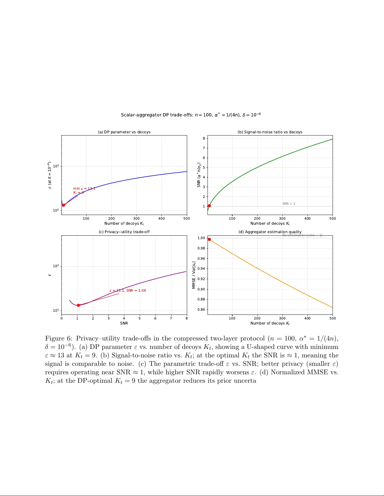
Com binatorial Priv acy: Priv ate Multi-P art y Bitstream Grand Sum b y Hiding in Birkhoﬀ P olytop es Praneeth V epakomma Mohamed bin Za yed Univ ersity of Artiﬁcial In telligence (MBZUAI) Massac husetts Institute of T ec hnology (MIT) vepakom@mit.edu Abstract W e in tro duce P olyV eil, a protocol for priv ate aggregation across k clien ts that enco des priv ate bits as p erm utation matrices in the Birkhoﬀ p olytop e. A t w o-la yer architecture gives the server p erfect sim ulation-based security (statistical distance zero) while a separate aggregator faces #P-hard lik eliho o d inference via the p ermanent and mixed discriminant. W e dev elop DP analyses under multiple frameworks (Berry–Esseen, R´ en yi, f-DP). In the full v arian t, where the aggregator sees a doubly sto chastic matrix p er client, the DP guarantee is non-v acuous only when the signal is undetectable. In the compressed v ariant, where the aggregator sees a scalar, f-DP gives ε ≈ 7 . 8 p er clien t. Sh uﬄe-mo del ampliﬁcation then yields ε ≈ 0 . 37 for k = 1 , 000 clients with no accuracy loss, since the aggregator needs only the sum of the shuﬄed scalars. This exp oses a tension b et ween #P-hardness (requiring the matrix view) and strong DP (requiring the sh uﬄed scalar view). F or the Bo olean sum alone, additiv e secret sharing dominates. The Birkhoﬀ enco ding’s adv an tage is multi-statistic extraction from a single matrix, enabling p er-bit marginals and w eigh ted sums without further client interaction. The proto col needs no PKI and outputs exact aggregates. Con ten ts 1 In tro duction 4 2 Related W ork 6 3 Preliminaries 7 3.1 Doubly Sto chastic Matrices and the Birkhoﬀ Polytope . . . . . . . . . . . . . . . . . 7 3.2 Uniform Sampling of Perm utation Matrices . . . . . . . . . . . . . . . . . . . . . . . 8 3.3 P ermutation Enco ding of Binary Data . . . . . . . . . . . . . . . . . . . . . . . . . . 8 3.4 Algebraic Bit Count Extraction . . . . . . . . . . . . . . . . . . . . . . . . . . . . . . 9 4 The P olyV eil Protocol 10 4.1 Problem Statemen t . . . . . . . . . . . . . . . . . . . . . . . . . . . . . . . . . . . . . 10 4.2 Threat Mo del . . . . . . . . . . . . . . . . . . . . . . . . . . . . . . . . . . . . . . . . 11 4.3 Proto col Description . . . . . . . . . . . . . . . . . . . . . . . . . . . . . . . . . . . . 12 4.4 Pro of of Correctness . . . . . . . . . . . . . . . . . . . . . . . . . . . . . . . . . . . . 13 4.5 In tegrity in the F ull Proto col . . . . . . . . . . . . . . . . . . . . . . . . . . . . . . . 13 4.6 Compressed V ariant . . . . . . . . . . . . . . . . . . . . . . . . . . . . . . . . . . . . 14 1 4.7 W orked Example with F ull Computation . . . . . . . . . . . . . . . . . . . . . . . . . 14 4.7.1 Ground T ruth . . . . . . . . . . . . . . . . . . . . . . . . . . . . . . . . . . . . 14 4.7.2 Clien t-Side Masking (F ull Detail for Clien t 1) . . . . . . . . . . . . . . . . . . 15 4.7.3 Clien t-Side Masking for Clients 2 and 3 (Summary) . . . . . . . . . . . . . . 16 4.7.4 Serv er-Side Extraction . . . . . . . . . . . . . . . . . . . . . . . . . . . . . . . 17 4.7.5 Secure Noise T ransmission . . . . . . . . . . . . . . . . . . . . . . . . . . . . . 17 4.7.6 Aggregation . . . . . . . . . . . . . . . . . . . . . . . . . . . . . . . . . . . . . 17 4.7.7 V eriﬁcation . . . . . . . . . . . . . . . . . . . . . . . . . . . . . . . . . . . . . 18 4.7.8 What the Server Cannot Do — De-Shuﬄing Analysis . . . . . . . . . . . . . 18 5 Securit y Analysis 19 5.1 The De-Sh uﬄing A ttac k (Compressed Proto col) . . . . . . . . . . . . . . . . . . . . . 19 5.2 Direct Inference from the Marginal (Compressed Proto col) . . . . . . . . . . . . . . . 20 5.3 Lik eliho o d Analysis of the F ull Proto col . . . . . . . . . . . . . . . . . . . . . . . . . 21 6 The Tw o-La yer PolyV eil Proto col 24 6.1 Arc hitecture Ov erview . . . . . . . . . . . . . . . . . . . . . . . . . . . . . . . . . . . 24 6.2 Correctness . . . . . . . . . . . . . . . . . . . . . . . . . . . . . . . . . . . . . . . . . 24 6.3 La yer 1: Information-Theoretic Security of the Server . . . . . . . . . . . . . . . . . 25 6.4 La yer 2: Computational Security of the Aggregator via #P-Hardness . . . . . . . . . 29 6.4.1 The Aggregator’s Inference Problem . . . . . . . . . . . . . . . . . . . . . . . 31 6.4.2 The Densit y of the Decoy Comp onent . . . . . . . . . . . . . . . . . . . . . . 31 6.4.3 Connection to the Permanen t . . . . . . . . . . . . . . . . . . . . . . . . . . . 32 6.4.4 Connection to the Mixed Discriminant . . . . . . . . . . . . . . . . . . . . . . 35 6.4.5 The F ormal Reduction . . . . . . . . . . . . . . . . . . . . . . . . . . . . . . . 36 6.4.6 The F ormal Hardness Statemen t . . . . . . . . . . . . . . . . . . . . . . . . . 36 6.4.7 Con trast with Gaussian Noise . . . . . . . . . . . . . . . . . . . . . . . . . . . 38 6.4.8 Wh y Appro ximate Permanen t Algorithms Do Not Help . . . . . . . . . . . . 38 6.5 F ormal Two-La yer Security Statement . . . . . . . . . . . . . . . . . . . . . . . . . . 39 7 Multi-Statistic Extraction from the Birkhoﬀ Enco ding 40 7.1 P er-Bit Marginal Coun ts . . . . . . . . . . . . . . . . . . . . . . . . . . . . . . . . . . 40 7.2 Arbitrary W eighted Sums . . . . . . . . . . . . . . . . . . . . . . . . . . . . . . . . . 41 7.3 Comparison with Additive Secret Sharing . . . . . . . . . . . . . . . . . . . . . . . . 42 8 Pro v able Aggregator Priv acy via An ti-Concen tration 42 8.1 Key Observ ation: ℓ ∞ Norm Do es Not Grow with n . . . . . . . . . . . . . . . . . . . 42 8.2 ( ε, δ )-DP via a High-Probabilit y Region . . . . . . . . . . . . . . . . . . . . . . . . . 43 8.3 Concen tration of R t : Finite-Sample Bound . . . . . . . . . . . . . . . . . . . . . . . 43 8.4 Restricted Log-Lipsc hitz Constan t on G r . . . . . . . . . . . . . . . . . . . . . . . . . 44 8.5 Finite-Sample CL T Error via Berry–Esseen . . . . . . . . . . . . . . . . . . . . . . . 45 8.6 Main Theorem: Finite-Sample ( ε, δ )-DP with Explicit Constants . . . . . . . . . . . 46 8.7 DP Analysis of the Compressed Two-La yer Proto col . . . . . . . . . . . . . . . . . . 48 8.7.1 Compressed Tw o-La yer Proto col . . . . . . . . . . . . . . . . . . . . . . . . . 48 8.7.2 Distribution of η t . . . . . . . . . . . . . . . . . . . . . . . . . . . . . . . . . . 49 8.7.3 Signal-to-Noise Ratio . . . . . . . . . . . . . . . . . . . . . . . . . . . . . . . . 50 8.7.4 ( ε, δ )-DP Guarantee for the Compressed Proto col . . . . . . . . . . . . . . . . 50 8.7.5 Summary of DP Results for the Compressed Proto col . . . . . . . . . . . . . 53 2 8.7.6 Aggregator Estimation Error (MMSE) . . . . . . . . . . . . . . . . . . . . . . 53 8.8 R ´ en yi Diﬀerential Priv acy . . . . . . . . . . . . . . . . . . . . . . . . . . . . . . . . . 55 8.8.1 R ´ en yi DP for the Compressed Proto col (Algorithm 4) . . . . . . . . . . . . . 55 8.8.2 R ´ en yi DP for the F ull Proto col (Algorithm 3) . . . . . . . . . . . . . . . . . . 56 8.8.3 Zero-Concen trated Diﬀeren tial Priv acy (zCDP) . . . . . . . . . . . . . . . . . 56 8.8.4 Gaussian Diﬀeren tial Priv acy (f-DP) . . . . . . . . . . . . . . . . . . . . . . . 57 8.9 Priv acy Ampliﬁcation b y Sh uﬄing . . . . . . . . . . . . . . . . . . . . . . . . . . . . 58 8.9.1 The Sh uﬄe Mo del . . . . . . . . . . . . . . . . . . . . . . . . . . . . . . . . . 58 8.9.2 Ampliﬁcation Bound . . . . . . . . . . . . . . . . . . . . . . . . . . . . . . . . 58 8.9.3 Numerical Ev aluation . . . . . . . . . . . . . . . . . . . . . . . . . . . . . . . 59 8.9.4 Prop erties of the Shuﬄed Compressed Proto col . . . . . . . . . . . . . . . . . 59 9 Conclusion 59 A Bac kground on Simulation-Based Security Pro ofs 61 A.1 The Problem That Simulation Solves . . . . . . . . . . . . . . . . . . . . . . . . . . . 61 A.2 F ormal Deﬁnition . . . . . . . . . . . . . . . . . . . . . . . . . . . . . . . . . . . . . . 61 A.3 How to Construct a Simulation Pro of . . . . . . . . . . . . . . . . . . . . . . . . . . 61 A.4 Why Simulation Implies Security . . . . . . . . . . . . . . . . . . . . . . . . . . . . . 62 A.5 Application to PolyV eil . . . . . . . . . . . . . . . . . . . . . . . . . . . . . . . . . . 62 B Analysis of A ttac k Strategies 65 B.0.1 Attac ks via Approximate Permanen t Algorithms . . . . . . . . . . . . . . . . 65 B.0.2 Quantitativ e Protection from Hardness of Approximation . . . . . . . . . . . 71 B.0.3 The Boundary Regime . . . . . . . . . . . . . . . . . . . . . . . . . . . . . . . 72 B.0.4 Boson Sampling and Quantum Attac ks . . . . . . . . . . . . . . . . . . . . . 73 B.0.5 W ork ed Example: The Reduction for n = 2 . . . . . . . . . . . . . . . . . . . 74 B.0.6 Why Lov´ asz–V empala V olume Algorithms Do Not Resolv e the Barrier . . . . 75 B.0.7 MCMC and Imp ortance Sampling A ttacks . . . . . . . . . . . . . . . . . . . . 75 B.0.8 Non-Likelihoo d Attac ks . . . . . . . . . . . . . . . . . . . . . . . . . . . . . . 76 3 1 In tro duction Computing aggregate statistics o ver priv ate data held b y man y parties is a foundational problem in priv acy-preserving computation. A concrete and widely applicable instance is the Bo olean sum problem, in which k clien ts each hold a priv ate binary string of length n and a server wishes to learn the total num b er of ones across all k n bits without learning an y individual client’s data. Applications range from epidemiological surv eillance, where a health authority counts p ositive test results without accessing individual diagnoses, to federated analytics, where a service pro vider tallies binary feature o ccurrences without centralizing user data. Existing approac hes to this problem broadly fall into three categories. Generic secure m ulti- part y computation (MPC) proto cols, built on garbled circuits or secret sharing, provide strong comp osable securit y with guaran tees based on sp eciﬁc computational hardness assumptions (suc h as the diﬃcult y of in teger factorization or the Learning with Errors problem o ver lattices), but imp ose communication and computation costs that scale with circuit complexity and b ecome pro- hibitiv e when k is large or netw ork conditions are constrained. Homomorphic encryption allo ws computation on ciphertexts, with securit y based on assumptions suc h as the comp osite residuosity problem (Paillier [5]) or the Learning with Errors problem (lattice-based FHE [6]), but carries sub- stan tial p er-op eration cost and requires careful k ey managemen t. Diﬀeren tial priv acy provides a framew ork for releasing aggregate statistics to un trusted parties b y adding calibrated noise, oﬀering formal ( ε, δ )-guarantees that hold regardless of an adversary’s computational p o w er, but inherently sacriﬁcing accuracy for priv acy . P olyV eil o ccupies a distinct p oint in this design space, one that we argue represen ts a new paradigm w e call Combinatorial Privacy . In P olyV eil, the core idea is to enco de eac h clien t’s priv ate bitstream as a p ermutation matrix, em b ed it inside a doubly stochastic matrix by mixing it with random decoy p erm utations, and use secure aggregation to reco v er the aggregate bit sum exactly . The Birkhoﬀ–von Neumann theorem guarantees that every doubly sto chastic matrix admits many decomp ositions into conv ex com binations of p ermutation matrices, and this non-uniqueness forms one of the tw o security lay ers of the proto col. W e presen t a rigorous securit y analysis that iden tiﬁes a fatal vulnerabilit y in naive implemen ta- tions of this approac h (the de-sh uﬄing attack, which recov ers all individual data with probability 1) and then dev elops a corrected two-layer pr oto c ol that ac hieves pro v able security . In the corrected proto col, the main serv er receiv es only aggregate scalars and is information-theoretically secure (its view is identically distributed for an y tw o inputs with the same aggregate). A separate aggregator en tity receives Birkhoﬀ-enco ded matrices but not the noise v alues, and faces a computational bar- rier: recov ering the priv ate permutation matrix from its enco ding requires ev aluating the densit y of a random doubly sto c hastic matrix at a given p oint, which we prov e is #P-hard via a reduction to the p ermanent. The tw o la y ers comp ose so that no single entit y can learn individual data: the serv er lac ks the information, and the aggregator lacks the computational p o wer. This tw o-lay er arc hitecture distinguishes Com binatorial Priv acy from existing paradigms. Un- lik e MPC and HE, whic h derive securit y from n um b er-theoretic hardness (factoring, L WE), PolyV eil’s computational la yer deriv es from the #P-hardness of ev aluating Birkhoﬀ p olytop e decomp osition lik eliho o ds (prov ed for lik eliho o d-based attacks; conjectured for all attacks). Unlik e DP , PolyV eil pro duces exact answers. The proto col requires no public-key infrastructure and has O ( k ) commu- nication in the compressed v ariant. 4 High-Lev el F ramew ork Figure 1 illustrates the t wo-la yer protoc ol at a high lev el. Eac h of the k clients holds a priv ate binary string b t ∈ { 0 , 1 } n . The proto col pro ceeds in three stages. Enc o ding. Eac h client enco des its bit vector b t as a block-diagonal p ermutation matrix M t ∈ { 0 , 1 } 2 n × 2 n and masks it b y forming the doubly sto chastic matrix D t = α ∗ M t + (1 − α ∗ ) R t , where R t is a random con vex combination of decoy p ermutation matrices. The client also computes the scalar f t = α ∗ s t + η t (where s t = P j b t,j is the bit coun t and η t is the noise from the decoys) and the noise v alue η t separately . Sep ar ation. The clien t sends D t (or f t in the compressed v arian t) to the aggregator, and η t to the noise aggregator. These t wo entities do not comm unicate with eac h other. The aggregator computes F = P t w T D t y (the aggregate of the bilinear extractions). The noise aggregator computes H = P t η t (the aggregate noise). Both scalars are sen t to the serv er. R e c overy. The server computes S = ( F − H ) /α ∗ , recov ering the exact Bo olean sum. The noise cancels algebraically: F − H = P t ( α ∗ s t + η t ) − P t η t = α ∗ S . The key prop erty is that no single en tity sees enough to learn individual data. The serv er sees only ( F , H ), whic h dep ends only on the aggregate S (information-theoretic securit y). The aggregator sees D t but not η t , so it cannot undo the noise cancellation; extracting M t from D t requires solving #P-hard problems (computational securit y). The noise aggregator sees η t but not D t or f t , so it learns nothing ab out b t . A single matrix D t enco des the en tire bit vector b t , not merely its sum. This means the aggregator can extract m ultiple statistics from the same data (per-bit marginals and weigh ted sums) without further clien t interaction, a capabilit y that additive secret sharing do es not provide for the same communication cost (Section 7). Clien t 1 b 1 Clien t 2 b 2 . . . Clien t k b k Birkhoﬀ Enco ding D t = α ∗ M t +(1 − α ∗ ) R t Aggregator F = P t w T D t y Noise Agg. H = P t η t Serv er S = F − H α ∗ D t or f t η t F H non-colluding Figure 1: The tw o-lay er PolyV eil proto col. Eac h client enco des its priv ate bit v ector as a masked doubly sto c hastic matrix D t and sends it (or the scalar f t ) to the aggregator, and the noise η t to a separate noise aggregator. The tw o aggregators do not communicate (dashed line). The serv er receiv es only the aggregate scalars F and H , from which it recov ers S exactly . The server has information-theoretic securit y (its view dep ends only on S ). The aggregator faces #P-hard inference (it sees D t but cannot eﬃciently extract M t ). The remainder of this paper is organized as follo ws. Section 3 establishes mathematical pre- liminaries. Section 4 presents the weak proto col v ariants and the de-shuﬄing attack. Section 5 pro vides security analysis. Section 6 develops the secure tw o-la yer protocol with pro ofs for both la yers. Section 7 derives multi-statistic extraction from the Birkhoﬀ encoding and compares with additiv e secret sharing. Section 8 pro ves a ﬁnite-sample ( ε, δ )-DP guaran tee for the aggregator, 5 analyzes the SNR regime where it is meaningful, and deriv es a non-v acuous ε for the compressed t wo-la yer proto col. Section 9 concludes. App endix A pro vides bac kground on sim ulation-based pro ofs. 2 Related W ork Secure multi-part y computation. The problem of computing functions o v er distributed pri- v ate inputs has b een studied since the foundational work of Y ao [1] on garbled circuits and Goldre- ic h, Micali, and Wigderson [2] on the GMW protocol. These generic constructions can compute an y function securely , including Bo olean sums, but their communication and computation costs scale with the circuit complexit y of the target function. More recen t framew orks suc h as SPDZ [3] reduce the online cost through prepro cessing, but the p er-gate ov erhead remains signiﬁcant compared to the simple arithmetic in P olyV eil. Sp ecialized secure aggregation proto cols suc h as that of Bona witz et al. [4] reduce comm unication th rough pairwise secret sharing and handle client drop out, ac hieving O ( k ) p er-client comm unication with O ( k 2 ) setup. P olyV eil ac hiev es O (1) p er-client comm unication (t wo scalars) in its compressed v arian t without pairwise key agreement. Homomorphic encryption. Additively homomorphic sc hemes suc h as Paillier [5] support addi- tiv e aggregation nativ ely . Each client encrypts their bit coun t under a common public k ey , the server m ultiplies ciphertexts, and a designated party decrypts the sum. This ac hieves exact results with IND-CP A securit y but requires public-k ey infrastructure. A P aillier ciphertext is t ypically 4096 bits at 128-bit security , whereas PolyV eil transmits a single scalar per client. F ully homomorphic encryption [6] generalizes to arbitrary computations but with substan tially greater o verhead. Diﬀeren tial priv acy . Diﬀeren tial priv acy [8] pro vides formal priv acy guaran tees through cali- brated noise. In the lo cal mo del, eac h clien t randomizes their data b efore sending it to the server, ac hieving priv acy without trust but with error Θ( √ k n/ε ). The cen tral mo del achiev es error Θ( n/ε ) but requires a trusted curator to see raw data. The sh uﬄe mo del [9, 10] interpolates by in terp osing an anon ymous shuﬄer, ac hieving cen tral-mo del accuracy with local-mo del trust. P olyV eil pro duces exact results and uses the same sh uﬄing infrastructure, but deriv es priv acy from algebraic masking rather than statistical noise. Instance mixing and data obfuscation. InstaHide [11] mixes priv ate data records with public datasets and random sign patterns for priv acy-preserving machine learning. While b oth InstaHide and PolyV eil in volv e mixing priv ate data with random elemen ts, PolyV eil focuses on aggregation rather than prediction, achiev es exact results through algebraic noise cancellation, and provides securit y guaran tees ro oted in the combinatorial structure of the Birkhoﬀ p olytop e. Secret sharing. Secret sharing sc hemes [13] distribute a secret among multiple parties so that only authorized subsets can reconstruct it. PolyV eil do es not use secret sharing directly but instead exploits the structure of doubly sto c hastic matrices so that the priv ate data is one of many v alid decomp ositions of a publicly shared matrix, creating a computational barrier for an y en tity that observ es the matrix but not the decomp osition co eﬃcien ts. 6 3 Preliminaries W e collect notation used throughout the pap er. All symbols are deﬁned in con text at ﬁrst use; this table serv es as a reference. Sym b ol Meaning n Num b er of bits p er client k Num b er of clients K t Num b er of decoy p ermutations for client t b t ∈ { 0 , 1 } n Clien t t ’s priv ate bit v ector s t = P j b t,j Bit coun t (Hamming weigh t) of b t S = P t s t T otal bit coun t (the target aggregate) Π( b ) 2 × 2 p erm utation matrix enco ding bit b M t = M ( b t ) 2 n × 2 n blo c k-diagonal p erm utation matrix enco ding b t P t,i i -th deco y p ermutation matrix for client t , uniform o ver S 2 n α ∗ Public w eigh t on the true enco ding in D t α t,i W eight on the i -th deco y ( P i α t,i = 1 − α ∗ ) D t Mask ed doubly sto c hastic matrix: α ∗ M t + P i α t,i P t,i R t Normalized deco y comp onent: ( D t − α ∗ M t ) / (1 − α ∗ ) w , y Extraction v ectors ( w 2 j − 1 = 1, w 2 j = 0; y 2 j − 1 = 0, y 2 j = 1) f t = w T D t y Extracted scalar: α ∗ s t + η t η t Noise in extracted scalar: (1 − α ∗ ) w T R t y ξ t,j P er-bit noise: (1 − α ∗ )( R t y ) 2 j − 1 F , H Aggregated signal and noise: F = P t f t , H = P t η t B m Birkhoﬀ p olytop e (set of m × m doubly sto chastic matrices) S m Symmetric group (set of all m ! p erm utation matrices of size m ) p erm( A ) P ermanen t of matrix A A ( R ′ ) Supp ort matrix: A ab = 1 [ R ′ ab > 0] Supp( R ′ ) Supp ort set: { Q ∈ S 2 n : Q ab = 1 ⇒ R ′ ab > 0 } ν ( R ′ ) Densit y of R t on B 2 n ev aluated at R ′ P ( σ 1 , . . . , σ K ; R ′ ) Co eﬃcien t p olytop e for a p erm utation tuple and target R ′ ε, δ Diﬀeren tial priv acy parameters µ Gaussian DP parameter: ∆ /σ η ρ zCDP parameter: ∆ 2 / (2 σ 2 ) 3.1 Doubly Sto chastic Matrices and the Birkhoﬀ P olytop e Deﬁnition 3.1 (Doubly sto chastic matrix) . A squar e matrix A = ( a ij ) ∈ R m × m with non-ne gative entries is doubly sto c hastic if every r ow and every c olumn sums to one, that is, P m j =1 a ij = 1 for al l i ∈ [ m ] , and P m i =1 a ij = 1 for al l j ∈ [ m ] . 7 Deﬁnition 3.2 (Birkhoﬀ p olytop e) . The Birkhoﬀ p olytop e B m is the set of al l m × m doubly sto chastic matric es. It is a c onvex p olytop e in R m × m of dimension ( m − 1) 2 . Theorem 3.3 (Birkhoﬀ–von Neumann [22, 23]) . The vertic es of B m ar e pr e cisely the m × m p er- mutation matric es. Every doubly sto chastic matrix A ∈ B m c an b e written as a c onvex c ombination of p ermutation matric es A = r X i =1 θ i P i , θ i > 0 , r X i =1 θ i = 1 , wher e e ach P i is a p ermutation matrix. This is a Birkhoﬀ–von Neumann (BvN) decomp osition of A . BvN decomp ositions are generically non-unique : a doubly sto chastic matrix in the in terior of B m admits man y distinct decomp ositions. Theorem 3.4 (Decomp osition m ultiplicit y , Brualdi [19]) . L et A ∈ B m have p p ositive entries. The numb er of distinct BvN de c omp ositions of A is at le ast p 2 . Theorem 3.5 (Marcus–Ree [20]) . Every m × m doubly sto chastic matrix c an b e expr esse d as a c onvex c ombination of at most m 2 − 2 m + 2 p ermutation matric es. Finding a BvN de c omp osition with the minimum numb er of p ermutations is NP-har d [21]. 3.2 Uniform Sampling of P erm utation Matrices A m × m p ermutation matrix P corresponds bijectively to a p ermutation σ ∈ S m (the symmetric group on [ m ] = { 1 , . . . , m } ) via P ij = 1 [ σ ( i ) = j ]. That is, row i of P has its unique 1 in column σ ( i ). T o draw P uniformly at r andom fr om S m , one draws a uniformly random p erm utation σ and constructs the corresp onding matrix. The standard algorithm for dra wing a uniform random p erm utation is the Fisher–Y ates s h uﬄe (also kno wn as the Knuth sh uﬄe): starting from the identit y p ermutation σ = (1 , 2 , . . . , m ), for i = m, m − 1 , . . . , 2, draw j uniformly at random from { 1 , . . . , i } and swap σ ( i ) ↔ σ ( j ). This pro duces eac h of the m ! permutations with equal probabilit y 1 /m ! and runs in O ( m ) time using O ( m ) random bits (sp eciﬁcally P m i =2 ⌈ log 2 i ⌉ bits). F or our proto col with m = 2 n , eac h random p erm utation matrix costs O ( n ) time and O ( n log n ) random bits. 3.3 P ermutation Enco ding of Binary Data Deﬁnition 3.6 (Bit-to-p ermutation enco ding) . F or a bit b ∈ { 0 , 1 } , deﬁne the 2 × 2 p ermutation matrix Π( b ) =            I 2 = 1 0 0 1 ! if b = 0 , J 2 = 0 1 1 0 ! if b = 1 . F or a bitstr e am b = ( b 1 , . . . , b n ) ∈ { 0 , 1 } n , deﬁne the blo ck-diagonal enc o ding M ( b ) = blo ckdiag  Π( b 1 ) , Π( b 2 ) , . . . , Π( b n )  ∈ { 0 , 1 } 2 n × 2 n . Since eac h Π( b j ) is a 2 × 2 p erm utation matrix, their blo ck-diagonal assem bly M ( b ) is a 2 n × 2 n p erm utation matrix and a v ertex of B 2 n . The block-diagonal structure conﬁnes eac h bit to a disjoin t 2 × 2 blo c k, enabling the algebraic extraction we now develop. 8 Example 3.7 (Enco ding of a 2-bit stream) . Consider the bitstr e am b = (1 , 0) with n = 2 . The enc o ding pr o duc es M  (1 , 0)  = blo c kdiag(Π(1) , Π(0)) = blo c kdiag  0 1 1 0  ,  1 0 0 1  =     0 1 0 0 1 0 0 0 0 0 1 0 0 0 0 1     . The ﬁrst 2 × 2 blo ck (r ows 1–2, c olumns 1–2) enc o des b 1 = 1 as the swap matrix J 2 . The se c ond 2 × 2 blo ck (r ows 3–4, c olumns 3–4) enc o des b 2 = 0 as the identity I 2 . A l l entries outside these blo cks ar e zer o due to the blo ck-diagonal structur e. 3.4 Algebraic Bit Count Extraction The bilinear form w T A y , applied to a doubly sto c hastic matrix A , extracts a scalar that dep ends on the structure of A . When A = M ( b ) is a permutation encoding of a bit v ector, appropriate c hoices of w and y reco ver the bit coun t, individual bits, or weigh ted combinations of bits. W e call ( w , y ) an extr action ve ctor p air , as they extract a target statistic from the enco ded matrix. Diﬀeren t extraction vector pairs applied to the same matrix yield diﬀerent statistics, which is the basis for the multi-statistic extraction developed in Section 7. Deﬁnition 3.8 (Extraction vectors for the bit coun t) . Deﬁne w , y ∈ R 2 n by w i = ( 1 if i is o dd , 0 if i is even , y i = ( 0 if i is o dd , 1 if i is even . Equivalently, w = (1 , 0 , 1 , 0 , . . . , 1 , 0) T and y = (0 , 1 , 0 , 1 , . . . , 0 , 1) T , e ach of length 2 n . Lemma 3.9 (Bit count extraction) . F or any bitstr e am b = ( b 1 , . . . , b n ) ∈ { 0 , 1 } n with p ermutation enc o ding M = M ( b ) w T M y = n X j =1 b j . Pr o of. W e compute w T M y by expanding the matrix-v ector pro ducts step by step. Computing M y . Since M = blo c kdiag (Π( b 1 ) , . . . , Π( b n )) is blo c k-diagonal, the pro duct M y decomp oses in to indep endent block m ultiplications. F or the j -th blo ck, the relev ant entries of y are y 2 j − 1 = 0 and y 2 j = 1. W riting y j = ( y 2 j − 1 , y 2 j ) T = (0 , 1) T for the p ortion of y corresp onding to blo ck j , we hav e Π( b j ) y j = Π( b j )  0 1  . When b j = 0: Π(0)  0 1  =  1 0 0 1   0 1  =  0 1  . When b j = 1: Π(1)  0 1  =  0 1 1 0   0 1  =  1 0  . Therefore, the en tries of M y at p ositions 2 j − 1 and 2 j are ( M y ) 2 j − 1 = b j , ( M y ) 2 j = 1 − b j . (1) T o verify this: when b j = 0, ( M y ) 2 j − 1 = 0 = b j and ( M y ) 2 j = 1 = 1 − b j . When b j = 1, ( M y ) 2 j − 1 = 1 = b j and ( M y ) 2 j = 0 = 1 − b j . Both cases match (1). 9 Computing w T ( M y ) . Now we take the inner pro duct of w with M y w T ( M y ) = 2 n X i =1 w i ( M y ) i = n X j =1 h w 2 j − 1 ( M y ) 2 j − 1 + w 2 j ( M y ) 2 j i = n X j =1 h 1 · b j + 0 · (1 − b j ) i = n X j =1 b j , (2) where the third equalit y substitutes w 2 j − 1 = 1, w 2 j = 0 from Deﬁnition 3.8 and ( M y ) 2 j − 1 = b j , ( M y ) 2 j = 1 − b j from (1). The key mechanism is that w “selects” only the o dd-indexed entries of M y , each of which equals the corresp onding bit b j . Example 3.10 (Extraction for a concrete bitstream) . T ake n = 2 , b = (1 , 0) . Then w = (1 , 0 , 1 , 0) T and y = (0 , 1 , 0 , 1) T . F r om Example 3.7 M =     0 1 0 0 1 0 0 0 0 0 1 0 0 0 0 1     . First c ompute M y M y =     0 1 0 0 1 0 0 0 0 0 1 0 0 0 0 1         0 1 0 1     =     0 · 0 + 1 · 1 + 0 · 0 + 0 · 1 1 · 0 + 0 · 1 + 0 · 0 + 0 · 1 0 · 0 + 0 · 1 + 1 · 0 + 0 · 1 0 · 0 + 0 · 1 + 0 · 0 + 1 · 1     =     1 0 0 1     . Che cking against (1) , for blo ck j = 1 ( b 1 = 1 ): ( M y ) 1 = 1 = b 1 and ( M y ) 2 = 0 = 1 − b 1 . F or blo ck j = 2 ( b 2 = 0 ): ( M y ) 3 = 0 = b 2 and ( M y ) 4 = 1 = 1 − b 2 . Both match. Now c ompute w T ( M y ) w T ( M y ) = (1 , 0 , 1 , 0)     1 0 0 1     = 1 · 1 + 0 · 0 + 1 · 0 + 0 · 1 = 1 . The r esult is 1 = b 1 + b 2 = 1 + 0 , c onﬁrming the lemma. 4 The P olyV eil Proto col 4.1 Problem Statemen t W e consider k client en tities, where client t ∈ [ k ] holds a priv ate binary bitstream b t = ( b t, 1 , . . . , b t,n ) ∈ { 0 , 1 } n of length n . Let s t = P n j =1 b t,j denote the n um b er of ones in client t ’s bitstream. The goal is for a server to compute the aggregate S = P k t =1 s t without learning an y individual s t , an y individual bitstream b t , or any partial aggregates inv olving fewer than all k clien ts. 10 4.2 Threat Mo del W e op erate in the honest-but-curious (semi-honest) mo del, deﬁned as follo ws. Serv er b eha vior. The serv er executes every instruction of the proto col exactly as sp eciﬁed. It do es not deviate from the proto col b y , for example, sending altered intermediate results to clien ts, injecting false data, or failing to perform a required computation. How ev er, the serv er records ev ery message it receives and may subsequen tly p erform arbitrary p olynomial-time computations on this recorded transcript in an attempt to infer individual client data. The serv er’s computational p ow er is bounded only b y p olynomial time; it may run brute-force searc hes ov er feasible spaces, solve optimization problems, and apply any statistical inference tec hnique. The securit y guarantees we pro ve hold against an y suc h p olynomial-time analysis. Comm unication security . All comm unication c hannels b etw een each clien t and the server, and b et w een eac h client and the sh uﬄer, are authen ticated and encrypted using standard transp ort- la yer security (e.g., TLS 1.3). Authentication ensures that the server receives messages only from legitimate clien ts and not from imp ersonators. Encryption ensures that no external eav esdropp er observing the net work can read the conten t of any message. T ogether, these guarantees mean that the only en tity that sees a client’s message to the serv er is the serv er itself, and the only entit y that sees a clien t’s message to the sh uﬄer is the sh uﬄer itself. W e do not assume that the comm unication c hannels hide metadata suc h as message timing or size. Clien t b ehavior. Ev ery client follo ws the proto col faithfully . No clien t mo diﬁes, omits, or fabri- cates an y message. No clien t shares its priv ate data, its random coins, or its intermediate computa- tions with the serv er or with any other client (b eyond what the proto col prescrib es). In particular, no client colludes with the server to de-anonymize the sh uﬄed v alues. The non-collusion assump- tion is essential, since if ev en one client shared its η t v alue directly with the server (outside the sh uﬄe), the serv er could link that η t to the client’s identit y and compute s t = ( f t − η t ) /α ∗ . T rusted sh uﬄer. There exists a functionalit y F shuﬄe that operates as follows. It accepts as input one scalar v alue from each of the k clien ts, collecting the m ultiset { η 1 , . . . , η k } . It then applies a p erm utation π dra wn uniformly at random from the symmetric group S k (the set of all k ! bijections on [ k ]), and outputs the p ermuted sequence ( η π (1) , . . . , η π ( k ) ) to the server. Critically , the serv er learns the v alues in the output sequence but do es not learn the permutation π . This means that for any position j in the output, the server kno ws the v alue η π ( j ) but cannot determine which clien t submitted it. The shuﬄer do es not rev eal π to the clients either. This ideal functionality can b e instan tiated in sev eral w ays. The simplest is a non-c ol luding auxiliary server : a separate ph ysical serv er, operated b y an indep endent party that does not collude with the main server, receiv es all η t v alues, permutes them, and forwards the result. A stronger instan tiation is a mixnet , where each client encrypts its v alue under lay ered encryption addressed to a chain of rela y serv ers, each of whic h p eels one encryption lay er and shuﬄes the messages. V eriﬁable mixnets [14] additionally produce a zero-knowledge pro of that the output is a v alid p erm utation of the input, preven ting a malicious relay from altering v alues. A fully cryptographic instan tiation uses a multi-p arty shuﬄing pr oto c ol suc h as the secret-shared shuﬄe of Chase, Ghosh, and Poburinna ya [14], whic h distributes the shuﬄing computation among t wo or more servers so that no single server learns the p ermutation, ac hieving securit y even if one serv er is corrupted. 11 W e require k ≥ 3 to ensure that the sh uﬄe provides meaningful anon ymit y . With k = 1, the sh uﬄed output c on tains a single v alue that is trivially link ed to the sole client. With k = 2, the serv er has a 1 / 2 probability of guessing the correct assignmen t, providing negligible priv acy . 4.3 Proto col Description The proto col uses a public parameter α ∗ ∈ (0 , 1) that controls the trade-oﬀ betw een signal strength and priv acy , as smaller α ∗ hides M t more deeply in the in terior of B 2 n but requires greater numerical precision to recov er S . Algorithm 1 PolyV eil Public parameters: bit length n , scaling factor α ∗ ∈ (0 , 1), extraction vectors w , y (Deﬁni- tion 3.8). Client-Side Masking 1: for each client t ∈ { 1 , . . . , k } in parallel do 2: Enco de priv ate bitstream as M t = M ( b t ) ∈ { 0 , 1 } 2 n × 2 n via Deﬁnition 3.6. 3: Cho ose K t ≥ 2 and draw K t uniformly random p ermutation matrices P t, 1 , . . . , P t,K t from S 2 n using the Fisher–Y ates sh uﬄe (Section 3.2). 4: Sample p ositive co eﬃcients α t, 1 , . . . , α t,K t > 0 with P K t i =1 α t,i = 1 − α ∗ . 5: Construct the masked matrix: D t = α ∗ M t + K t X i =1 α t,i P t,i . (3) 6: Compute the noise term: η t = K t X i =1 α t,i  w T P t,i y  . (4) 7: Send D t to the server. 8: end for Ser ver-Side Extra ction 9: for each client t ∈ { 1 , . . . , k } do 10: Serv er computes: f t = w T D t y . (5) 11: end for Secure Noise Transmission 12: Eac h client t submits scalar η t to the trusted shuﬄer F shuﬄe . 13: Sh uﬄer draws π ∼ S k and sends ( η π (1) , . . . , η π ( k ) ) to server. A ggrega tion 14: Serv er computes: S = 1 α ∗ k X t =1 f t − k X t =1 η t ! . (6) 12 4.4 Pro of of Correctness Theorem 4.1 (Correctness) . A lgorithm 1 c omputes S = P k t =1 s t exactly. Pr o of. The matrix M t = M ( b t ) is a permutation matrix (Deﬁnition 3.6) and hence doubly stochas- tic: each row and column con tains exactly one 1 and the rest 0, so all row sums and column sums equal 1. Eac h P t,i is a p erm utation matrix dra wn uniformly from S 2 n and is lik ewise doubly sto c hastic. The co eﬃcien ts α ∗ , α t, 1 , . . . , α t,K t are strictly p ositive with α ∗ + P i α t,i = 1. Since B 2 n is con v ex and D t is a conv ex com bination of elements of B 2 n D t = α ∗ M t + K t X i =1 α t,i P t,i ∈ B 2 n . Applying the bilinear form A 7→ w T A y to D t and using linearit y of matrix-v ector m ultiplication f t = w T D t y = w T α ∗ M t + K t X i =1 α t,i P t,i ! y = α ∗ ( w T M t y ) + K t X i =1 α t,i ( w T P t,i y ) . (7) By Lemma 3.9, w T M t y = P n j =1 b t,j = s t . By deﬁnition (4), η t = P K t i =1 α t,i ( w T P t,i y ). Substituting, f t = α ∗ s t + η t . Summing o v er all k clients, k X t =1 f t = k X t =1 ( α ∗ s t + η t ) = α ∗ k X t =1 s t + k X t =1 η t = α ∗ S + k X t =1 η t . The serv er kno ws P t f t from the extraction step. The sh uﬄed list ( η π (1) , . . . , η π ( k ) ) is a p ermutation of ( η 1 , . . . , η k ), and the sum is inv ariant under p ermutation, so P k j =1 η π ( j ) = P k t =1 η t . Therefore the serv er can compute S = 1 α ∗ k X t =1 f t − k X t =1 η t ! = 1 α ∗ α ∗ S + X t η t − X t η t ! = 1 α ∗ · α ∗ S = S, conﬁrming that the proto col outputs the correct aggregate. 4.5 In tegrity in the F ull Proto col In the full (non-compressed) proto col, the serv er receiv es the matrix D t directly and computes f t = w T D t y itself. A malicious client cannot cause the serv er to use an incorrect f t b ecause the serv er p erforms the extraction indep endently . Sp eciﬁcally , ev en if a client wished to inﬂate or deﬂate its contribution to the aggregate, the client can only control what matrix D t it sends. The serv er then computes f t = w T D t y deterministically from D t , so the client cannot make the serv er b eliev e a diﬀerent f t than the one implied by the submitted D t . 13 The server can additionally verify that the receiv ed D t is a v alid doubly stochastic matrix b y c hecking that all entries are non-negativ e and that ev ery ro w and column sums to 1 (within ﬂoating- p oin t tolerance). If a client submits a matrix that is not doubly sto chastic, the server can reject it. This v eriﬁcation do es not reveal the clien t’s priv ate data (since an y doubly sto chastic matrix passes the c heck, regardless of whic h permutation is hidden inside), but it prev ents malformed submissions that could corrupt the aggregate. The remaining vulnerabilit y is that a malicious clien t could submit a v alid doubly sto c hastic matrix D t that enco des a bitstream diﬀerent from its true b t . This is the standard “input substi- tution” attack in the semi-honest mo del, where a dishonest clien t lies about its data. Prev enting this requires mechanisms b eyond the semi-honest mo del, such as zero-knowledge pro ofs that D t is correctly constructed from the client’s certiﬁed data source. W e do not address this in the current w ork. 4.6 Compressed V arian t Algorithm 2 PolyV eil (Compressed) Public parameter: α ∗ ∈ (0 , 1), extraction vectors w , y . 1: for each client t ∈ { 1 , . . . , k } in parallel do 2: Compute s t = P n j =1 b t,j lo cally . 3: Dra w random p erm utations P t, 1 , . . . , P t,K t and co eﬃcients α t,i > 0 with P i α t,i = 1 − α ∗ . 4: Compute η t = P i α t,i ( w T P t,i y ). 5: Compute f t = α ∗ s t + η t . 6: Send f t to serv er. 7: end for 8: Clien ts jointly sh uﬄe { η 1 , . . . , η k } and deliver to server. 9: Serv er computes S = 1 α ∗  P t f t − P t η t  . The compressed v ariant oﬀers three concrete adv antages b ey ond the communication reduction from O ( n 2 ) to O (1) p er clien t. First, the serv er never sees the doubly sto chastic matrix D t , whic h eliminates the BvN decomp osition as an attack v ector, as the serv er has no matrix to decomp ose. Second, client-side computation drops from O ( n 2 ) (constructing a 2 n × 2 n matrix) to O ( nK t ) (generating K t random permutations and computing K t bilinear forms). Third, serv er computation drops from O ( k n 2 ) to O ( k ), b ecoming indep endent of the bitstream length. The trade-oﬀ is that a malicious client can send an arbitrary f t without the server b eing able to verify it, since the serv er no longer has D t to chec k. Under the semi-honest mo del this is not a concern. 4.7 W orked Example with F ull Computation W e trace ev ery computation explicitly for k = 3 clients, n = 2 bits, α ∗ = 0 . 3. 4.7.1 Ground T ruth Clien t 1 holds b 1 = (1 , 0), so s 1 = 1. Client 2 holds b 2 = (1 , 1), so s 2 = 2. Client 3 holds b 3 = (0 , 1), so s 3 = 1. The true aggregate is S = 1 + 2 + 1 = 4. The public parameters are n = 2, α ∗ = 0 . 3, w = (1 , 0 , 1 , 0) T , y = (0 , 1 , 0 , 1) T . 14 4.7.2 Clien t-Side Masking (F ull Detail for Clien t 1) Enco ding M 1 . Client 1’s bitstream is (1 , 0). Applying Deﬁnition 3.6 M 1 = blo c kdiag(Π(1) , Π(0)) = blo c kdiag  0 1 1 0  ,  1 0 0 1  =     0 1 0 0 1 0 0 0 0 0 1 0 0 0 0 1     . Generating deco y p erm utations. Client 1 chooses K 1 = 2 deco y p ermutations drawn uni- formly from S 4 (the symmetric group on { 1 , 2 , 3 , 4 } ). Supp ose the Fisher–Y ates sh uﬄe pro duces P ermutation σ 1 = (3 , 1 , 4 , 2), meaning σ 1 (1) = 3, σ 1 (2) = 1, σ 1 (3) = 4, σ 1 (4) = 2. The corresp onding p ermutation matrix has P 1 , 1 [ i, σ 1 ( i )] = 1 P 1 , 1 =     0 0 1 0 1 0 0 0 0 0 0 1 0 1 0 0     . V eriﬁcation that this is correct — row 1 has its 1 in column 3 (since σ 1 (1) = 3); row 2 in column 1; ro w 3 in column 4; row 4 in column 2. Each row and column has exactly one 1. P ermutation σ 2 = (2 , 1 , 4 , 3) P 1 , 2 =     0 1 0 0 1 0 0 0 0 0 0 1 0 0 1 0     . T o verify , row 1 has 1 in column 2; row 2 in column 1; row 3 in column 4; row 4 in column 3. Cho osing co eﬃcients. Clien t 1 samples α 1 , 1 = 0 . 5 and α 1 , 2 = 0 . 2, satisfying α 1 , 1 + α 1 , 2 = 0 . 7 = 1 − 0 . 3 = 1 − α ∗ . Constructing D 1 . Applying equation (3): D 1 = α ∗ M 1 + α 1 , 1 P 1 , 1 + α 1 , 2 P 1 , 2 = 0 . 3 M 1 + 0 . 5 P 1 , 1 + 0 . 2 P 1 , 2 . Computing eac h scaled matrix, 0 . 3 M 1 =     0 0 . 3 0 0 0 . 3 0 0 0 0 0 0 . 3 0 0 0 0 0 . 3     , 0 . 5 P 1 , 1 =     0 0 0 . 5 0 0 . 5 0 0 0 0 0 0 0 . 5 0 0 . 5 0 0     , 0 . 2 P 1 , 2 =     0 0 . 2 0 0 0 . 2 0 0 0 0 0 0 0 . 2 0 0 0 . 2 0     . Summing en try b y en try , D 1 =     0 + 0 + 0 0 . 3 + 0 + 0 . 2 0 + 0 . 5 + 0 0 + 0 + 0 0 . 3 + 0 . 5 + 0 . 2 0 + 0 + 0 0 + 0 + 0 0 + 0 + 0 0 + 0 + 0 0 + 0 + 0 0 . 3 + 0 + 0 0 + 0 . 5 + 0 . 2 0 + 0 + 0 0 + 0 . 5 + 0 0 + 0 + 0 . 2 0 . 3 + 0 + 0     =     0 0 . 5 0 . 5 0 1 . 0 0 0 0 0 0 0 . 3 0 . 7 0 0 . 5 0 . 2 0 . 3     . 15 T o verify that D 1 is doubly sto c hastic, the row sums are 0 + 0 . 5 + 0 . 5 + 0 = 1, 1 + 0 + 0 + 0 = 1, 0 + 0 + 0 . 3 + 0 . 7 = 1, 0 + 0 . 5 + 0 . 2 + 0 . 3 = 1. The column sums are 0 + 1 + 0 + 0 = 1, 0 . 5 + 0 + 0 + 0 . 5 = 1, 0 . 5 + 0 + 0 . 3 + 0 . 2 = 1, 0 + 0 + 0 . 7 + 0 . 3 = 1. All en tries are non-negativ e. Computing η 1 . Applying equation (4): η 1 = α 1 , 1 ( w T P 1 , 1 y ) + α 1 , 2 ( w T P 1 , 2 y ). F or P 1 , 1 P 1 , 1 y =     0 0 1 0 1 0 0 0 0 0 0 1 0 1 0 0         0 1 0 1     =     0 0 1 1     , w T ( P 1 , 1 y ) = (1 , 0 , 1 , 0)     0 0 1 1     = 0 + 0 + 1 + 0 = 1 . F or P 1 , 2 P 1 , 2 y =     0 1 0 0 1 0 0 0 0 0 0 1 0 0 1 0         0 1 0 1     =     1 0 1 0     , w T ( P 1 , 2 y ) = (1 , 0 , 1 , 0)     1 0 1 0     = 1 + 0 + 1 + 0 = 2 . Therefore, η 1 = 0 . 5 × 1 + 0 . 2 × 2 = 0 . 5 + 0 . 4 = 0 . 9. Clien t 1 sends D 1 to the server and holds η 1 = 0 . 9 for the shuﬄe. 4.7.3 Clien t-Side Masking for Clien ts 2 and 3 (Summary) Clien t 2. Bitstream b 2 = (1 , 1), s 2 = 2. M 2 = blo c kdiag(Π(1) , Π(1)) =     0 1 0 0 1 0 0 0 0 0 0 1 0 0 1 0     . Supp ose Client 2 dra ws P 2 , 1 corresp onding to σ = (4 , 3 , 2 , 1) and P 2 , 2 corresp onding to σ = (1 , 2 , 3 , 4) (the identit y), with α 2 , 1 = 0 . 4, α 2 , 2 = 0 . 3 P 2 , 1 =     0 0 0 1 0 0 1 0 0 1 0 0 1 0 0 0     , P 2 , 2 =     1 0 0 0 0 1 0 0 0 0 1 0 0 0 0 1     . Then D 2 = 0 . 3 M 2 + 0 . 4 P 2 , 1 + 0 . 3 P 2 , 2 . Compute w T P 2 , 1 y P 2 , 1 y =     1 0 1 0     , w T     1 0 1 0     = 2 . Compute w T P 2 , 2 y P 2 , 2 y = y =     0 1 0 1     , w T y = 0 . So η 2 = 0 . 4 × 2 + 0 . 3 × 0 = 0 . 8. 16 Clien t 3. Bitstream b 3 = (0 , 1), s 3 = 1. M 3 = blo c kdiag(Π(0) , Π(1)) =     1 0 0 0 0 1 0 0 0 0 0 1 0 0 1 0     . Supp ose Clien t 3 dra ws P 3 , 1 from σ = (2 , 1 , 3 , 4) and P 3 , 2 from σ = (3 , 4 , 1 , 2), with α 3 , 1 = 0 . 35, α 3 , 2 = 0 . 35 P 3 , 1 =     0 1 0 0 1 0 0 0 0 0 1 0 0 0 0 1     , P 3 , 2 =     0 0 1 0 0 0 0 1 1 0 0 0 0 1 0 0     . P 3 , 1 y = (1 , 0 , 0 , 1) T , so w T ( P 3 , 1 y ) = 1 · 1 + 0 · 0 + 1 · 0 + 0 · 1 = 1. P 3 , 2 y = (0 , 1 , 0 , 1) T , so w T ( P 3 , 2 y ) = 0. η 3 = 0 . 35 × 1 + 0 . 35 × 0 = 0 . 35. 4.7.4 Serv er-Side Extraction The serv er computes f t = w T D t y for each client. By the decomp osition prov ed in equation (7) of Theorem 4.1 (namely , that the bilinear extraction w T D t y equals α ∗ s t + η t due to the linearity of the bilinear form and Lemma 3.9), we hav e F or Client 1: f 1 = α ∗ s 1 + η 1 = 0 . 3 × 1 + 0 . 9 = 1 . 2. W e verify this b y direct computation on D 1 D 1 y =     0 0 . 5 0 . 5 0 1 . 0 0 0 0 0 0 0 . 3 0 . 7 0 0 . 5 0 . 2 0 . 3         0 1 0 1     =     0 . 5 0 0 . 7 0 . 8     . f 1 = w T ( D 1 y ) = (1 , 0 , 1 , 0)(0 . 5 , 0 , 0 . 7 , 0 . 8) T = 1 · 0 . 5 + 0 · 0 + 1 · 0 . 7 + 0 · 0 . 8 = 1 . 2 . F or Client 2: f 2 = α ∗ s 2 + η 2 = 0 . 3 × 2 + 0 . 8 = 1 . 4. F or Client 3: f 3 = α ∗ s 3 + η 3 = 0 . 3 × 1 + 0 . 35 = 0 . 65. 4.7.5 Secure Noise T ransmission Eac h client submits its η t to the shuﬄer. Clien t 1 submits η 1 = 0 . 9, Client 2 submits η 2 = 0 . 8, Client 3 submits η 3 = 0 . 35. The sh uﬄer draws a uniformly random p ermutation π ∈ S 3 ; supp ose π = (2 , 3 , 1) (meaning π (1) = 2, π (2) = 3, π (3) = 1). The server receiv es the sequence ( η π (1) , η π (2) , η π (3) ) = ( η 2 , η 3 , η 1 ) = (0 . 8 , 0 . 35 , 0 . 9). The server sees the v alues 0 . 8, 0 . 35, 0 . 9 but do es not kno w that 0 . 8 came from Client 2, 0 . 35 from Client 3, and 0 . 9 from Client 1. 4.7.6 Aggregation The server applies equation (6), which states S = 1 α ∗ ( P k t =1 f t − P k t =1 η t ). This form ula w as deriv ed in Theorem 4.1 from the fact that f t = α ∗ s t + η t (equation (7)), so P t f t − P t η t = α ∗ P t s t , and dividing b y α ∗ reco vers P t s t . 17 The serv er computes 3 X t =1 f t = 1 . 2 + 1 . 4 + 0 . 65 = 3 . 25 . 3 X t =1 η t = 0 . 8 + 0 . 35 + 0 . 9 = 2 . 05 . (sum is the same regardless of shuﬄe order) S = 1 0 . 3 (3 . 25 − 2 . 05) = 1 . 2 0 . 3 = 4 . 4.7.7 V eriﬁcation The ground truth is S = s 1 + s 2 + s 3 = 1 + 2 + 1 = 4. The proto col output matc hes. T o see why the cancellation works algebraically X t f t − X t η t = ( f 1 − η 1 ) + ( f 2 − η 2 ) + ( f 3 − η 3 ) (note: repairing the sum by the iden tity f t = α ∗ s t + η t for eac h t ) = α ∗ s 1 + α ∗ s 2 + α ∗ s 3 = α ∗ ( s 1 + s 2 + s 3 ) = 0 . 3 × 4 = 1 . 2 . Dividing by α ∗ = 0 . 3 gives 4. This cancellation holds for an y v alues of the η t ’s, an y num b er of deco y permutations, and an y p ositiv e coeﬃcients, b ecause it depends solely on the algebraic iden tity f t − η t = α ∗ s t . 4.7.8 What the Server Cannot Do — De-Sh uﬄing Analysis The server knows f 1 = 1 . 2, f 2 = 1 . 4, f 3 = 0 . 65 (linked to clien t identities) and the s h uﬄed v alues { 0 . 8 , 0 . 35 , 0 . 9 } (unlink ed). T o learn individual s t v alues, the serv er m ust assign each shuﬄed η -v alue to the correct clien t. There are 3! = 6 possible assignmen ts (since the three v alues are distinct), and the server can test each. Assignmen t σ ˆ s 1 = f 1 − η σ (1) α ∗ ˆ s 2 = f 2 − η σ (2) α ∗ ˆ s 3 = f 3 − η σ (3) α ∗ All ˆ s t ∈ { 0 , 1 , 2 } ? (0 . 8 , 0 . 35 , 0 . 9) 0 . 4 0 . 3 = 1 . 33 1 . 05 0 . 3 = 3 . 50 − 0 . 25 0 . 3 = − 0 . 83 No (0 . 8 , 0 . 9 , 0 . 35) 1 . 33 1 . 67 1 . 00 No (0 . 35 , 0 . 8 , 0 . 9) 2 . 83 2 . 00 − 0 . 83 No (0 . 35 , 0 . 9 , 0 . 8) 2 . 83 1 . 67 − 0 . 50 No (0 . 9 , 0 . 35 , 0 . 8) 1 . 00 3 . 50 − 0 . 50 No (0 . 9 , 0 . 8 , 0 . 35) 1 . 00 2 . 00 1 . 00 Y es In this example, only one assignmen t yields v alid bit counts (integers in { 0 , . . . , n } ). This is a consequence of the small parameters ( n = 2, k = 3). With larger n and k , m ultiple assignmen ts will pro duce v alid integer coun ts summing to S , and the server cannot distinguish among them. W e analyze this formally in Section 5. The probability that the server guesses the correct assignment is 1 /k ! = 1 / 6 by random guess- ing alone. How ev er, as we show in Section 5, the server can exploit the integralit y constraint s t ∈ { 0 , . . . , n } to identify the correct assignmen t with probability 1, rendering the naive proto col insecure. 18 T o prev en t de-sh uﬄing , the protocol relies on the trusted sh uﬄer F shuﬄe (Section 4.2), whic h guaran tees that the p erm utation π is uniformly random and unknown to the server. As we analyze rigorously in Section 5, this sh uﬄing alone is not suﬃcient to prev en t the serv er from reco vering individual s t v alues, b ecause of an integralit y constraint that enables deterministic de-shuﬄing. This motiv ates the proto col mo diﬁcations presented in Section 6. 5 Securit y Analysis W e provide a rigorous securit y analysis of the basic proto col v ariants (Algorithms 1 and 2). W e iden tify fundamen tal vulnerabilities in both v ariants, quan tify the information leak age precisely , and defer the corrected proto cols to Section 6. 5.1 The De-Sh uﬄing A ttac k (Compressed Proto col) The compressed proto col has the server receive identit y-linked scalars f t = α ∗ s t + η t for t ∈ [ k ] and the sh uﬄed sequence ( ˜ η 1 , . . . , ˜ η k ) = ( η π (1) , . . . , η π ( k ) ). Theorem 5.1 (De-sh uﬄing via in tegralit y constraint) . In the c ompr esse d pr oto c ol, the server c an r e c over every client’s bit c ount s t with pr ob ability 1 (over the pr oto c ol’s r andomness). Pr o of. The serv er observ es t w o sets of data, namely iden tit y-link ed scalars (1 , f 1 ) , (2 , f 2 ) , . . . , ( k , f k ) where f t = α ∗ s t + η t , and shuﬄed noise ( ˜ η 1 , . . . , ˜ η k ) = ( η π (1) , . . . , η π ( k ) ) for unknown π ∈ S k . The server’s test. F or eac h candidate bijection σ : [ k ] → [ k ], the server computes ˆ s t ( σ ) = f t − ˜ η σ ( t ) α ∗ , t = 1 , . . . , k , and c hec ks whether ˆ s t ( σ ) ∈ { 0 , 1 , . . . , n } for all t sim ultaneously . The true assignment p asses the test. Let σ ∗ = π − 1 b e the true assignment (i.e., ˜ η σ ∗ ( t ) = η t for all t ). Then ˆ s t ( σ ∗ ) = f t − ˜ η σ ∗ ( t ) α ∗ = f t − η t α ∗ = ( α ∗ s t + η t ) − η t α ∗ = s t . Since s t = P n j =1 b t,j ∈ { 0 , 1 , . . . , n } , all k candidate v alues pass the integralit y test. A ny wr ong assignment fails with pr ob ability 1. Let σ  = σ ∗ . There exists some t 0 ∈ [ k ] with σ ( t 0 )  = σ ∗ ( t 0 ). Let j = π ( σ ( t 0 )) b e the client whose η -v alue is at p osition σ ( t 0 ) in the shuﬄed sequence, so ˜ η σ ( t 0 ) = η j with j  = t 0 . Then ˆ s t 0 ( σ ) = f t 0 − η j α ∗ = α ∗ s t 0 + η t 0 − η j α ∗ = s t 0 + η t 0 − η j α ∗ . (8) This equals an integer if and only if ( η t 0 − η j ) /α ∗ is an integer, i.e., η t 0 − η j ∈ α ∗ Z . No w w e sho w Pr[ η t 0 − η j ∈ α ∗ Z ] = 0. Each η t = P K t i =1 α t,i X t,i where X t,i = w T P t,i y ∈ { 0 , 1 , . . . , n } are integer-v alued and the co eﬃcients α t,i are dra wn from a contin uous distribution on { ( α 1 , . . . , α K t ) : α i > 0 , P i α i = 1 − α ∗ } . Consider the conditional distribution of η t 0 giv en all other randomness (including η j and the integer v alues X t 0 ,i ). Conditional on X t 0 , 1 , . . . , X t 0 ,K t 0 , the random v ariable η t 0 = P i α t 0 ,i X t 0 ,i is a linear function of the contin uously distributed co eﬃcients ( α t 0 , 1 , . . . , α t 0 ,K t 0 ). Since the X t 0 ,i are not all equal (with probability 1, as the permutations are 19 dra wn indep endently and uniformly), this linear function is non-constant, so η t 0 has a contin uous conditional distribution. Therefore Pr[ η t 0 − η j ∈ α ∗ Z ] = Pr[ η t 0 ∈ η j + α ∗ Z ] = 0 , since a contin uous random v ariable assigns probability zero to any countable set. Uniqueness and c onclusion. Since σ ∗ passes the test and eac h σ  = σ ∗ fails with probabilit y 1, taking a union b ound ov er the (ﬁnite) set of k ! − 1 wrong assignmen ts Pr[an y wrong σ passes] ≤ X σ  = σ ∗ Pr[ σ passes] = 0 . Therefore, with probability 1, the server uniquely identiﬁes σ ∗ and recov ers s t = ˆ s t ( σ ∗ ) for all t ∈ [ k ]. Remark 5.2 (This attack is demonstrated in the work ed example) . The worke d example in Se c- tion 4.7 il lustr ates this attack explicitly. The server tests al l 3! = 6 assignments of shuﬄe d η values to clients and ﬁnds that exactly one assignment yields valid bit c ounts ( s 1 , s 2 , s 3 ) = (1 , 2 , 1) with al l s t ∈ { 0 , 1 , 2 } . The p ap er pr eviously describ e d this as a sp e cial c ase for smal l n , but The or em 5.1 shows it works for al l n . 5.2 Direct Inference from the Marginal (Compressed Protocol) Ev en without de-sh uﬄing, the serv er can p erform Bay esian inference on s t from f t alone. Prop osition 5.3 (Serv er’s p osterior from f t ) . L et µ denote the pr ob ability density of η t (which is c ontinuous and indep endent of b t ). The server’s p osterior distribution over s t given f t is Pr( s t = s | f t ) = µ ( f t − α ∗ s ) · π ( s ) P n s ′ =0 µ ( f t − α ∗ s ′ ) · π ( s ′ ) , (9) wher e π ( s ) is any prior distribution over s t ∈ { 0 , 1 , . . . , n } . Pr o of. W e derive this from Ba y es’ theorem. The serv er kno ws f t and seeks s t . Since f t = α ∗ s t + η t and η t is indep enden t of s t with densit y µ , the conditional density of f t giv en s t = s tak es the form p ( f t | s t = s ) = p ( α ∗ s + η t = f t ) = p ( η t = f t − α ∗ s ) = µ ( f t − α ∗ s ) . The second equalit y uses the deterministic relationship f t = α ∗ s + η t , so ﬁxing s t = s means η t = f t − α ∗ s . Applying Bay es’ theorem with prior π ( s ) = Pr( s t = s ) Pr( s t = s | f t ) = p ( f t | s t = s ) · π ( s ) p ( f t ) = µ ( f t − α ∗ s ) · π ( s ) P n s ′ =0 µ ( f t − α ∗ s ′ ) · π ( s ′ ) , where the denominator is the marginal density p ( f t ) = P n s ′ =0 p ( f t | s t = s ′ ) π ( s ′ ), obtained b y the la w of total probabilit y ov er the ( n + 1) p ossible v alues of s t . The MAP (maximum a p osteriori) estimator selects the s that maximizes the numerator. F or a uniform prior, this reduces to ˆ s t = arg max s µ ( f t − α ∗ s ). 20 Remark 5.4 (This channel is weak for small α ∗ , but irrelev an t given de-sh uﬄing) . When α ∗ is smal l r elative to the standar d deviation of η t , the density µ ( f t − α ∗ s ) varies slow ly with s and the p osterior is ne arly uniform. T o se e this, we c ompute std( η t ) . Each term w T P t,i y = P n j =1 ( P t,i ) 2 j − 1 , 2 j , which c ounts the numb er of 2 × 2 diagonal blo cks in which P t,i maps the o dd index to the even index. F or a uniform r andom p ermutation matrix, e ach ( P t,i ) 2 j − 1 , 2 j is a Bernoul li r andom variable, and w T P t,i y ∈ { 0 , 1 , . . . , n } . Its exp e ctation is E [ w T P t,i y ] = n X j =1 E [( P t,i ) 2 j − 1 , 2 j ] = n X j =1 1 2 n = n 2 n = 1 2 . T o se e this, note that w T P y extr acts the sum of entries at p ositions (1 , 2) , (3 , 4) , (5 , 6) , . . . , (2 n − 1 , 2 n ) . F or a uniform r andom p ermutation σ , ( P ) 2 j − 1 , 2 j = 1 [ σ (2 j − 1) = 2 j ] , and Pr[ σ (2 j − 1) = 2 j ] = 1 / (2 n ) . Summing over j = 1 , . . . , n gives n/ (2 n ) = 1 / 2 . The varianc e involves c orr elations b etwe en blo cks, but for lar ge n is appr oximately n · 1 2 n (1 − 1 2 n ) ≈ 1 / 2 . Ther efor e V ar[ w T P y ] = Θ(1) and std[ w T P y ] = Θ(1) . Now η t = P K t i =1 α t,i ( w T P t,i y ) . Its me an is E [ η t ] = K t X i =1 α t,i · 1 2 = 1 − α ∗ 2 . Its varianc e (c onditional on c o eﬃcients, using indep endenc e of the P t,i ) is V ar[ η t ] = K t X i =1 α 2 t,i · V ar[ w T P t,i y ] = Θ(1) · K t X i =1 α 2 t,i . F or K t r oughly uniform weights, P i α 2 t,i ≈ (1 − α ∗ ) 2 /K t , giving std[ η t ] = Θ((1 − α ∗ ) / √ K t ) . The signal (diﬀer enc e b etwe en f t for adjac ent s values) is α ∗ . The total signal r ange acr oss al l n + 1 p ossible s t values is α ∗ n . The signal-to-noise r atio for distinguishing s t fr om s t + 1 is SNR = α ∗ std[ η t ] = α ∗ √ K t (1 − α ∗ ) · Θ(1) . F or α ∗ = 1 / (4 n ) and K t = O (1) , this is O (1 /n ) , making the p er-unit SNR ne gligible. However, this analysis is mo ot b e c ause the de-shuﬄing attack of The or em 5.1 r e c overs s t with pr ob ability 1 r e gar d less of the signal-to-noise r atio. 5.3 Lik eliho o d Analysis of the F ull Proto col In the full proto col, the server additionally receives D t = α ∗ M t + (1 − α ∗ ) R t , where R t ∼ ν is the random decoy c omp onen t. The server can compute the likelihoo d of each candidate p ermutation matrix M ′ Prop osition 5.5 (P osterior concen tration in the full protocol) . L et ν denote the distribution of R t = 1 1 − α ∗ P i α t,i P t,i over B 2 n . F or e ach c andidate M ′ ∈ L ( D t , α ∗ ) , the likeliho o d is Pr( D t | M t = M ′ ) = 1 (1 − α ∗ ) d ν  D t − α ∗ M ′ 1 − α ∗  , wher e d is the dimension of B 2 n . As K t → ∞ , the p osterior pr ob ability of the true M t appr o aches 1. 21 Pr o of. Deriving the likeliho o d. The mask ed matrix is D t = α ∗ M t + (1 − α ∗ ) R t , where R t ∼ ν . F or a candidate M ′ , deﬁne the residual R ′ = ( D t − α ∗ M ′ ) / (1 − α ∗ ). W e wan t Pr( D t | M t = M ′ ). Since D t = α ∗ M ′ + (1 − α ∗ ) R t when M t = M ′ , the even t { D t = d } is the ev ent { R t = ( d − α ∗ M ′ ) / (1 − α ∗ ) } . The map φ : R 7→ α ∗ M ′ + (1 − α ∗ ) R is an aﬃne transformation from B 2 n to itself. Its Jacobian matrix is (1 − α ∗ ) I d where d = (2 n − 1) 2 is the dimension of B 2 n (a doubly sto chastic matrix has (2 n ) 2 en tries but (2 n − 1) 2 degrees of freedom after enforcing ro w and column sum constraints). The absolute v alue of the Jacobian determinant is | det((1 − α ∗ ) I d ) | = (1 − α ∗ ) d . By the standard c hange-of-v ariables formula for densities, if R t has densit y ν ( R ), then D t = φ ( R t ) has density p ( d | M t = M ′ ) = 1 (1 − α ∗ ) d ν  d − α ∗ M ′ 1 − α ∗  = 1 (1 − α ∗ ) d ν ( R ′ ) . The true r esidual was dr awn fr om ν ; false r esiduals wer e not. F or the true M t , the residual is R = D t − α ∗ M t 1 − α ∗ = ( α ∗ M t + (1 − α ∗ ) R t ) − α ∗ M t 1 − α ∗ = R t , whic h w as drawn from ν b y construction. F or any M ′  = M t R ′ = D t − α ∗ M ′ 1 − α ∗ = ( α ∗ M t + (1 − α ∗ ) R t ) − α ∗ M ′ 1 − α ∗ = R t + α ∗ ( M t − M ′ ) 1 − α ∗ = R + α ∗ 1 − α ∗ ( M t − M ′ ) . Since M t  = M ′ , the matrix M t − M ′ is nonzero (it has en tries in {− 1 , 0 , 1 } with at least t wo nonzero en tries), so R ′ is a translate of R b y a ﬁxed nonzero shift. Computing E [ P ij ] for a uniform r andom p ermutation matrix. Let P b e a uniform random p erm utation matrix in S 2 n , corresp onding to a p ermutation σ drawn uniformly from the symmetric group S 2 n . The ( i, j ) entry of P is the indicator P ij = 1 [ σ ( i ) = j ]. Since σ is uniform o v er all (2 n )! p erm utations E [ P ij ] = Pr[ σ ( i ) = j ] = |{ σ ∈ S 2 n : σ ( i ) = j }| | S 2 n | = (2 n − 1)! (2 n )! = 1 2 n . The numerator coun ts the p ermutations that map i to j : once σ ( i ) = j is ﬁxed, the remaining 2 n − 1 elements can b e mapp ed in (2 n − 1)! wa ys. Therefore E [ P ] = 1 2 n J , where J is the (2 n ) × (2 n ) all-ones matrix. (One can v erify that eac h row of E [ P ] sums to (2 n ) · 1 2 n = 1, consisten t with P b eing doubly sto chastic.) Computing V ar[ P ij ] . Since P ij = 1 [ σ ( i ) = j ] ∈ { 0 , 1 } is a Bernoulli random v ariable with parameter p = 1 / (2 n ) V ar[ P ij ] = p (1 − p ) = 1 2 n  1 − 1 2 n  = 2 n − 1 (2 n ) 2 . Conc entr ation of R t as K t → ∞ . Each entry of R t is ( R t ) ab = 1 1 − α ∗ K t X i =1 α t,i ( P t,i ) ab . 22 Its exp ectation is E [( R t ) ab ] = 1 1 − α ∗ K t X i =1 α t,i E [( P t,i ) ab ] = 1 1 − α ∗ K t X i =1 α t,i · 1 2 n = 1 1 − α ∗ · 1 2 n K t X i =1 α t,i = 1 1 − α ∗ · 1 2 n · (1 − α ∗ ) = 1 2 n , where w e used P K t i =1 α t,i = 1 − α ∗ . Its v ariance is (using indep endence of the P t,i and treating α t,i as ﬁxed conditional on the co eﬃcien t dra w) V ar[( R t ) ab ] = 1 (1 − α ∗ ) 2 K t X i =1 α 2 t,i V ar[( P t,i ) ab ] = 1 (1 − α ∗ ) 2 K t X i =1 α 2 t,i · 2 n − 1 (2 n ) 2 . F or roughly uniform weigh ts α t,i ≈ (1 − α ∗ ) /K t , w e hav e P i α 2 t,i ≈ K t · ((1 − α ∗ ) /K t ) 2 = (1 − α ∗ ) 2 /K t . Substituting, V ar[( R t ) ab ] ≈ 1 (1 − α ∗ ) 2 · (1 − α ∗ ) 2 K t · 2 n − 1 (2 n ) 2 = 2 n − 1 (2 n ) 2 K t = 1 K t · 1 2 n  1 − 1 2 n  . The standard deviation in each entry is therefore std[( R t ) ab ] = O (1 / √ K t ). By Cheb yshev’s in- equalit y applied en try-wise, for an y ε > 0 Pr      ( R t ) ab − 1 2 n     > ε  ≤ V ar[( R t ) ab ] ε 2 = O  1 K t ε 2  → 0 as K t → ∞ . Hence R t → 1 2 n J in probability , entry-wise. Likeliho o d r atio diver ges. The true residual R satisﬁes ∥ R − 1 2 n J ∥ ∞ = O P (1 / √ K t ) (where ∥ · ∥ ∞ is the max entry). The false residual satisﬁes     R ′ − 1 2 n J     ∞ =     R − 1 2 n J + α ∗ 1 − α ∗ ( M t − M ′ )     ∞ . The shift matrix α ∗ 1 − α ∗ ( M t − M ′ ) has entries of magnitude α ∗ 1 − α ∗ at the p ositions where M t and M ′ diﬀer. Since M t  = M ′ (they diﬀer in at least 2 rows), w e hav e     R ′ − 1 2 n J     ∞ ≥ α ∗ 1 − α ∗ − O P  1 √ K t  . F or K t large enough that 1 / √ K t ≪ α ∗ / (1 − α ∗ ), the false residual R ′ lies at distance Θ( α ∗ / (1 − α ∗ )) from the mode 1 2 n J , while R lies at distance O (1 / √ K t ). Since ν concen trates with width O (1 / √ K t ), the false residual is Θ( α ∗ √ K t / (1 − α ∗ )) standard deviations from the mo de. Therefore ν ( R ′ ) /ν ( R ) → 0 as K t → ∞ (assuming α ∗ is ﬁxed), and the likelihoo d ratio div erges ν ( R ) ν ( R ′ ) → ∞ as K t → ∞ . Applying Ba y es’ theorem with a uniform prior π ( M ′ ) = 1 / (2 n )! for all M ′ ∈ S 2 n Pr( M t = M ′ | D t ) = ν ( R ′ ) P M ′′ ∈ S 2 n ν ( R ′′ ) → ( 1 if M ′ = M t , 0 if M ′  = M t , since the numerator for M ′ = M t dominates all other terms. Remark 5.6 (More deco ys can decrease securit y) . This cr e ates a c ounterintuitive tr ade-oﬀ. In- cr e asing K t (adding mor e de c oy p ermutations) was intende d to impr ove se curity by incr e asing the de c omp osition c ount L . However, incr e asing K t also c onc entr ates ν , making the likeliho o d r atio ν ( R ) /ν ( R ′ ) lar ger and the server’s MAP estimate mor e ac cur ate. A gainst a c omputational ly un- b ounde d adversary, the c onc entr ation eﬀe ct dominates the de c omp osition-c ount eﬀe ct. 23 6 The Tw o-La y er P olyV eil Proto col The de-sh uﬄing attack (Theorem 5.1) sho ws that no proto col v ariant in which the serv er sees iden tity-link ed f t v alues and sh uﬄed η t v alues separately can b e secure. The root cause is that the integralit y constrain t s t ∈ { 0 , . . . , n } allows the server to uniquely identify the true shuﬄe p erm utation. W e no w presen t a corrected protocol with a two-layer architecture in which no single en tity can learn individual data. The design addresses the reviewer critique that any aggregation-only proto col (where the serv er sees only P f t and P η t ) is trivially secure and do es not require the Birkhoﬀ p olytop e. In our t wo-la yer proto col, the Birkhoﬀ enco ding is essential for the security of the aggregation lay er. 6.1 Arc hitecture Ov erview The protocol inv olves three types of en tities: Clien ts t ∈ [ k ], eac h holding priv ate b t ∈ { 0 , 1 } n ; an Aggregator A , whic h receiv es mask ed matrices D t and computes the scalar aggregate F = P t w T D t y , which it sends to the serv er (the aggregator do es not receiv e η t v alues); and a Server S , whic h receiv es F from the aggregator and H = P t η t from a separate noise-aggregation channel, and computes S = ( F − H ) /α ∗ . The key design principle is sep ar ation of information : the aggregator sees D t (whic h enco des M t ) but not η t ; a separate c hannel deliv ers P η t to the serv er without the aggregator’s in v olv ement. Algorithm 3 Two-La y er P olyV eil Public parameters: n , α ∗ ∈ (0 , 1), w , y . En tities: Aggregator A , noise aggregator B , server S . Client-Side Comput a tion 1: for each client t ∈ [ k ] in parallel do 2: Enco de M t = M ( b t ). Draw K t ≥ 2 uniform random p ermutations P t,i ∈ S 2 n . 3: Sample α t, 1 , . . . , α t,K t > 0 with P i α t,i = 1 − α ∗ . 4: Compute D t = α ∗ M t + P i α t,i P t,i and η t = P i α t,i ( w T P t,i y ). 5: Send D t to aggregator A . Send η t to noise aggregator B . 6: end for A ggrega tion 7: A computes F = P k t =1 w T D t y and sends F to server S . 8: B computes H = P k t =1 η t and sends H to serv er S . 9: S computes S = ( F − H ) /α ∗ . 6.2 Correctness Theorem 6.1 (Correctness) . A lgorithm 3 outputs S = P t s t exactly. 24 Pr o of. The aggregator computes F = k X t =1 w T D t y = k X t =1 w T α ∗ M t + K t X i =1 α t,i P t,i ! y = k X t =1 α ∗ ( w T M t y ) + K t X i =1 α t,i ( w T P t,i y ) ! = k X t =1 ( α ∗ s t + η t ) = α ∗ k X t =1 s t + k X t =1 η t = α ∗ S + H , where w e used Lemma 3.9 ( w T M t y = s t ) and the deﬁnition η t = P i α t,i ( w T P t,i y ). The noise aggregator computes H = P k t =1 η t indep enden tly . The serv er receiv es F and H and computes F − H α ∗ = ( α ∗ S + H ) − H α ∗ = α ∗ S α ∗ = S. 6.3 La yer 1: Information-Theoretic Securit y of the Server The server S receiv es only t wo scalars: the aggregate signal F = P t f t and the aggregate noise H = P t η t . W e pro ve that the serv er learns nothing ab out any individual clien t’s data b eyond the aggregate S = P t s t , using the simulation paradigm from secure multi-part y computation (bac kground in App endix A). The idea of a sim ulation proof is simple: w e construct an algorithm (the simulator ) that can fabricate a fake server view using only the aggregate S and public parameters — without knowing any individual input b t . If the fabricated view is distributed iden tically to the real view, then the real view contains no information about individual inputs beyond S , b ecause anything the server could compute from the real view, it could equally compute from the sim ulator’s output (which dep ends only on S ). Figure 2 illustrates the pro of structure. Theorem 6.2 (P erfect sim ulation-based security of the serv er) . L et D = ( b 1 , . . . , b k ) and D ′ = ( b ′ 1 , . . . , b ′ k ) b e any two input c onﬁgur ations satisfying P t s t = P t s ′ t = S . Then: (i) The server’s view ( F , H ) under D and ( F , H ) under D ′ have identic al distributions. (ii) Ther e exists a simulator S sim that, given only S and the public p ar ameters ( k , n, α ∗ ) , outputs a p air ( ˆ F , ˆ H ) with ( ˆ F , ˆ H ) ≡ ( F , H ) (identic al distributions) for al l inputs with aggr e gate S . The pro of pro ceeds in four stages. Pr o of. Stage 1: The noise η t is independent of the priv ate input b t . This is the structural prop erty on which the en tire pro of rests. Each client’s noise is η t = K t X i =1 α t,i ( w T P t,i y ) , where P t, 1 , . . . , P t,K t are drawn uniformly and indep endently from S 2 n , and the co eﬃcients ( α t, 1 , . . . , α t,K t ) are dra wn from a contin uous distribution g on the simplex ∆ K t = { ( α 1 , . . . , α K t ) : α i > 0 , P i α i = 1 − α ∗ } . Crucially , neither the p erm utations P t,i nor the co eﬃcien ts α t,i dep end on b t — they are dra wn from distributions determined entirely by the public parameters ( n, K t , α ∗ ). 25 Real W orld Inputs: b 1 , . . . , b k (speciﬁc priv ate bit vectors) Protocol execution: Each client computes f t = α ∗ s t + η t where η t uses fresh random permutations + coeﬃcients. Server receives F = P f t , H = P η t . Server’s view: ( F, H ) = ( α ∗ S + H, H ) where H ∼ µ ∗ k independently of which b t produced S . Sim ulated W orld Input to simulator: S only (no individual b t v alues) Simulator S sim : Draw fresh random p ermutations and co eﬃcients. Compute ˆ η t for each t . Set ˆ H = P ˆ η t , ˆ F = α ∗ S + ˆ H . Simulator’s output: ( ˆ F , ˆ H ) = ( α ∗ S + ˆ H , ˆ H ) where ˆ H ∼ µ ∗ k (same distribution as real H ). ≡ identic al distributions (stat. distanc e = 0 ) Why it works: The noise η t depends only on the random p ermutations and coeﬃcients, not on b t . Therefore the simulator can generate ˆ η t with the same distribution as η t without knowing b t . The only place b t enters the server’s view is through the aggregate S = P s t , which the simulator knows. Figure 2: Structure of the sim ulation proof for the server’s information-theoretic security (The- orem 6.2). Left: the real protocol execution with actual priv ate inputs. Righ t: the simulator, whic h knows only the aggregate S (not individual b t ) and fabricates a view with identical distribu- tion. The equiv alence ≡ means identical distributions, holding against computationally unbounded adv ersaries. The dashed b ox states the key structural prop ert y that mak es the pro of work. 26 F ormally , let Ω t = S K t 2 n × ∆ K t denote the probability space of client t ’s randomness, equipped with the pro duct of the uniform measure on S K t 2 n and the distribution g on ∆ K t . The map ω t = ( P t, 1 , . . . , P t,K t , α t, 1 , . . . , α t,K t ) 7→ η t ( ω t ) = P i α t,i ( w T P t,i y ) is a measurable function of ω t alone. Since ω t is sampled from a distribution that do es not inv olv e b t , w e ha v e η t ⊥ ⊥ b t (statistical indep endence) . (10) Let µ denote the distribution of η t . This distribution is the same for every client (since the public parameters are shared) and do es not dep end on an y priv ate input. Since the randomness is also indep enden t across clients, the noise v alues η 1 , . . . , η k are m utually indep endent: ( η 1 , . . . , η k ) ∼ µ ⊗ k (i.i.d. from µ , indep endent of D ) . (11) Stage 2: The server’s view is a deterministic function of ( S, H ) . The serv er receiv es tw o scalars. The ﬁrst is F = k X t =1 f t = k X t =1 w T D t y = k X t =1 ( α ∗ s t + η t ) = α ∗ k X t =1 s t | {z } = S + k X t =1 η t | {z } = H = α ∗ S + H . (12) The second is H = P k t =1 η t directly . Therefore the serv er’s complete view is the pair View server = ( F , H ) = ( α ∗ S + H , H ) . (13) This is a deterministic, inv ertible function of ( S, H ): given ( F , H ), one recov ers S = ( F − H ) /α ∗ , and giv en ( S, H ), one reco v ers F = α ∗ S + H . The only randomness in the view comes from H . Stage 3: The distribution of the view dep ends only on S , not on which D pro duced S . By Stage 1, H = P k t =1 η t where η 1 , . . . , η k ∼ µ ⊗ k indep enden tly of D . The distribution of H is therefore the k -fold conv olution µ ∗ k : Pr[ H ∈ B | D ] = Pr[ H ∈ B ] = µ ∗ k ( B ) , ∀ D , ∀ measurable B ⊆ R . (14) By Stage 2, F = α ∗ S + H . F or any measurable set A ⊆ R 2 : Pr[( F , H ) ∈ A | D ] = Z R 1  ( α ∗ S + h, h ) ∈ A  dµ ∗ k ( h ) . (15) No w consider a diﬀerent input D ′ with P t s ′ t = S (the same aggregate). By exactly the same argumen t: Pr  ( F , H ) ∈ A | D ′  = Z R 1  ( α ∗ S + h, h ) ∈ A  dµ ∗ k ( h ) . The right-hand sides are identical: the integrand dep ends only on S (whic h is the same for D and D ′ ), and the measure µ ∗ k is indep endent of the input conﬁguration. Therefore Pr[( F , H ) ∈ A | D ] = Pr  ( F , H ) ∈ A | D ′  , ∀ measurable A, whic h is statement (i): iden tical distributions. The statistical distance b etw een the t wo views is exactly zero. Stage 4: Constructing the sim ulator. W e now build the sim ulator S sim that pro duces a fake view from S alone: 27 Input: The aggregate S and public parameters ( k , n, α ∗ , K t ). (a) F or each t = 1 , . . . , k : draw K t indep enden t uniform random permutations ˆ P t,i ∈ S 2 n and co eﬃcien ts ( ˆ α t, 1 , . . . , ˆ α t,K t ) from the distribution g on ∆ K t . (b) Compute ˆ η t = P K t i =1 ˆ α t,i ( w T ˆ P t,i y ) for eac h t . (c) Compute ˆ H = P k t =1 ˆ η t . (d) Compute ˆ F = α ∗ S + ˆ H . Output: ( ˆ F , ˆ H ). The sim ulator uses fresh randomness (the ˆ P t,i and ˆ α t,i ) that is indep endent of the actual protocol execution. It do es not know an y b t , an y s t , an y D t , or any η t . It knows only S . W e verify that the sim ulator’s output has the correct distribution. By construction, ˆ η 1 , . . . , ˆ η k are i.i.d. from µ (since each is generated b y the same random process as the real η t ). Therefore ˆ H = P t ˆ η t has distribution µ ∗ k , and ( ˆ F , ˆ H ) = ( α ∗ S + ˆ H , ˆ H ) . Comparing with (15): for any measurable A , Pr h ( ˆ F , ˆ H ) ∈ A i = Z R 1  ( α ∗ S + h, h ) ∈ A  dµ ∗ k ( h ) = Pr[( F , H ) ∈ A | D ] , for any input D with aggregate S . This is statemen t (ii): S sim ( S ) ≡ ( F , H ). Remark 6.3 (What the simulator pro of means concretely) . The simulator demonstr ates that ev- erything the server se es — the aggr e gate signal F and the aggr e gate noise H — c ould have b e en gener ate d by an algorithm that knows nothing ab out any individual client. The server c annot dis- tinguish the r e al pr oto c ol (wher e actual clients submitte d actual private data) fr om the simulate d pr oto c ol (wher e a single machine fabric ate d fake aggr e gates fr om S alone). A ny function the server c omputes on its r e al view — any test statistic, any machine le arning mo del, any side-channel anal- ysis — it c ould e qual ly wel l c ompute on the simulator’s output, which c ontains zer o individual-level information. This is information-the or etic: it holds against adversaries with unlimite d c omputa- tional p ower, unlimite d memory, and unlimite d time. Remark 6.4 (Structural source of securit y) . The pr o of r elies on exactly one structur al pr op erty: η t ⊥ ⊥ b t (the noise is indep endent of the private data). Any noise gener ation pr o c ess with this pr op erty would give the server the same information-the or etic guar ante e. The Birkhoﬀ enc o ding, the p ermutation matric es, the BvN de c omp osition — none of these ar e ne e de d for the server’s se curity. They ar e ne e de d only for the aggr e gator’s c omputational b arrier (L ayer 2). The server’s se curity would hold even if the noise wer e Gaussian, L aplac e, or any other distribution, as long as it is indep endent of b t and c anc els exactly in the aggr e gate. 28 6.4 La yer 2: Computational Securit y of the Aggregator via #P-Hardness The aggregator A sees the individual matrices D 1 , . . . , D k but do es not receive η t or f t as separate scalars. T o reco v er clien t t ’s data, the aggregator must extract M t from D t = α ∗ M t + (1 − α ∗ ) R t . W e sho w that the natural approac h — computing the p osterior distribution o ver candidate permutation matrices — requires solving #P-hard problems. The argumen t connects the aggregator’s densit y ev aluation to three classical hard problems: the p ermanen t, p erfect matchings in bipartite graphs, and the mixed discriminant. Figure 3 pro vides a roadmap of the logical structure; the rest of this section ﬁlls in every detail. 1. The aggregator’s problem. Aggregator observes D t = α ∗ M t + (1 − α ∗ ) R t and w ants to reco ver M t . 2. Bay esian inference requires ev aluating ν ( R ′ ) . Pr( M t = M ′ | D t ) ∝ ν ( R ′ ), where R ′ = ( D t − α ∗ M ′ ) / (1 − α ∗ ) and ν is the density of the random decoy matrix R t on B 2 n . The MAP estimator picks the M ′ maximizing ν ( R ′ ). 3. The densit y is a sum ov er all p ermutation tuples. R t is built from K random permutations and random co eﬃcients. The density at R ′ sums o ver every possible tuple, weigh ted by the probability the co eﬃcients pro duce R ′ : ν ( R ′ ) = X all ((2 n )!) K tuples 1 ((2 n )!) K ×  integral of g ( α ) ov er α satisfying P i α i P σ i = (1 − α ∗ ) R ′  4. Most tuples con tribute zero. The constrain t P i α i P σ i = (1 − α ∗ ) R ′ with all α i > 0 forces: wherever R ′ ab = 0, no permutation in the tuple can hav e a 1 at ( a, b ). Each P σ i must “ﬁt inside” the positive en tries of R ′ . Only tuples where ev ery p ermutation lies in the supp ort set Supp( R ′ ) con tribute. 5. Rewrite the densit y using only v alid tuples. ν ( R ′ ) = C K ((2 n )!) K X ( σ 1 ,...,σ K ) ∈ Supp( R ′ ) K vol  P ( σ 1 , . . . , σ K ; R ′ )  This is a sum of p olytope volumes, one p er v alid tuple. Two questions arise: (a) Ho w many terms are in this sum? (b) What is eac h term (the polytop e volume)? These are answ ered in Figure 4. Figure 3: The density deriv ation: from the aggregator’s inference problem to the k ey formula. The aggregator’s MAP estimator requires ev aluating ν ( R ′ ) (Steps 1–2). The densit y marginalizes ov er all ((2 n )!) K p erm utation tuples (Step 3), but most contribute zero — only tuples in Supp( R ′ ) K surviv e (Step 4). The resulting formula (Step 5) is a sum of p olytop e v olumes o v er v alid tuples, raising t w o questions answ ered in Figure 4. W e b egin by establishing notation. Throughout this section, S m denotes the symmetric gr oup on m elements, i.e., the set of all m ! bijections σ : { 1 , . . . , m } → { 1 , . . . , m } . W e iden tify eac h bijection σ ∈ S m with the m × m p ermutation matrix P σ deﬁned by ( P σ ) ab = 1 [ σ ( a ) = b ], which has exactly one 1 in each row and eac h column and zeros everywhere else. The notation S 2 n th us refers to the set of all (2 n )! permutation matrices of size 2 n × 2 n , and S K 2 n = S 2 n × · · · × S 2 n ( K times) is the set of all ordered K -tuples of suc h matrices. 29 F rom Figure 3, Step 5: ν ( R ′ ) = C K ((2 n )!) K X Supp( R ′ ) K vol( P ) (a) Ho w many terms? (b) What is each term? Question (a): Ho w man y v alid tuples? Each of the K slots in ( σ 1 , . . . , σ K ) picks indep endently from Supp( R ′ ). Number of v alid tu- ples = | Supp( R ′ ) | K . Question (b): What is eac h volume? F or a v alid tuple, the constrain t P i α i P σ i = (1 − α ∗ ) R ′ de- ﬁnes a polytop e P ⊂ R K . The term equals C K · v ol( P ). | Supp( R ′ ) | equals the p ermanent. Deﬁne A ab = 1 [ R ′ ab > 0]. A permutation matrix Q “ﬁts inside” A iﬀ Q ab = 1 only where A ab = 1. This is a perfe ct matching in the bipartite graph G ( A ) (rows ↔ columns, edges where A ab = 1). | Supp( R ′ ) | = p erm( A ( R ′ )). vol( P ) equals a mixed discriminan t. The polytop e P is the in tersection of the K -simplex with (2 n − 1) 2 hyperplanes from the constraint. Its v olume can b e expressed as a mixe d discriminant of matrices constructed from the K p ermutations (Minko wski–Bernstein theory). V aliant (1979): Computing perm( A ) for { 0 , 1 } matrices is #P-complete . ⇒ Counting the nonzero terms in ν ( R ′ ) is #P-hard. Barvinok (1997): Computing the mixed dis- criminant is #P-hard . ⇒ Evaluating each nonzero term in ν ( R ′ ) is #P-hard. Conclusion (Theorem 6.15): Sub-problems of lik eliho o d ev aluation are #P-hard. The densit y ν ( R ′ ) is a sum of p erm( A ) K terms, eac h a #P-hard p olytope volume. All terms are ≥ 0 (no cancellation, unlike the determinant). No known p oly-time shortcut. Figure 4: The tw o branc hes of the #P-hardness argument, contin uing from the densit y formula in Figure 3. Left branch (Question a): the num b er of v alid tuples equals the permanent of the supp ort matrix A ( R ′ ), whic h coun ts p erfect matchings in a bipartite graph; computing this is #P-complete (V aliant, 1979). Righ t branch (Question b): eac h v alid tuple’s con tribution is a p olytop e volume expressible as a mixed discriminant; computing this is #P-hard (Barvinok, 1997). Both branches conv erge: the density is a #P-hard n umber of individually #P-hard terms, with no cancellation. 30 6.4.1 The Aggregator’s Inference Problem Giv en D t , the aggregator seeks M t . Recall that D t = α ∗ M t + (1 − α ∗ ) R t , so for any candidate p erm utation matrix M ′ , the aggregator can compute the r esidual R ′ = ( D t − α ∗ M ′ ) / (1 − α ∗ ). If M ′ happ ens to b e the true enco ding M t , then R ′ = R t (the actual random deco y matrix, which is doubly sto chastic by construction). If M ′ is wrong, R ′ ma y or ma y not b e doubly sto c hastic. The set of consistent candidates is therefore L ( D t , α ∗ ) = { M ′ ∈ S 2 n : R ′ := ( D t − α ∗ M ′ ) / (1 − α ∗ ) ∈ B 2 n } . The condition R ′ ∈ B 2 n requires ev ery entry R ′ ab to be non-negative (the row and column sum constrain ts are automatically satisﬁed since both D t and M ′ are doubly stochastic). Since ( M ′ ) ab ∈ { 0 , 1 } , the non-negativit y condition R ′ ab ≥ 0 is equiv alent to ( D t ) ab ≥ α ∗ at ev ery p osition ( a, b ) where M ′ has a 1. When α ∗ is small and the decoy comp onen t co vers all matrix entries (whic h happ ens with high probability for moderate K t ), the smallest entry of D t exceeds α ∗ and every p erm utation matrix in S 2 n is consistent: L ( D t , α ∗ ) = S 2 n . In this interior regime, consistency alone pro vides no information — all (2 n )! candidates lo ok equally v alid. The aggregator’s b est strategy , giv en unlimited computation, is Bay esian inference. Assuming a uniform prior ov er M ′ ∈ S 2 n , the p osterior probability of each candidate is Pr( M t = M ′ | D t ) = ν ( R ′ ) P M ′′ ∈L ν ( R ′′ ) , (16) where ν ( R ′ ) denotes the probability density of the random decoy matrix R t ev aluated at the p oint R ′ . The aggregator’s MAP (maxim um a p osteriori) estimator pic ks the candidate M ′ that maxi- mizes ν ( R ′ ). W e no w sho w that ev aluating ν ( R ′ ) is #P-hard. Remark 6.5 (Wh y fo cus on lik eliho o d, and what this do es not co ver) . The Bayesian/likeliho o d appr o ach is the statistically optimal attack: given unlimite d c omputation, no other metho d c an r e c over M t with higher pr ob ability. Pr oving it #P-har d ther efor e eliminates the str ongest p ossible attack str ate gy. However, this do es not rule out we aker but c omputational ly eﬃcient attacks that byp ass density evaluation entir ely. An aggr e gator might attempt sp e ctr al de c omp osition of D t , solve a line ar pr o gr am to ﬁnd a sp arse BvN de c omp osition, run the Hungarian algorithm on D t /α ∗ to ﬁnd the ne ar est p ermutation matrix, or tr ain a neur al network on synthetic ( D t , M t ) p airs. None of these r e quir e evaluating ν , and our #P-har dness r esult says nothing ab out them. We analyze sever al such non-likeliho o d attacks in App endix B and show that they fail at the pr oto c ol’s op er ating p ar ameters, but we do not pr ove a blanket imp ossibility r esult for al l p olynomial-time attacks. This gap is the c ontent of Conje ctur e B.14, which r emains op en. 6.4.2 The Densit y of the Deco y Comp onen t The decoy matrix R t is not drawn from a simple named distribution; it is constructed by a m ulti- step random pro cess. Understanding how ν ( R ′ ) arises from this pro cess is essential to the hardness argumen t, so w e deriv e the form ula in detail. Deﬁnition 6.6 (The random pro cess that generates R t ) . The de c oy matrix R t is gener ate d in two steps. First, dr aw K p ermutation matric es P σ 1 , . . . , P σ K indep endently and uniformly at r andom fr om S 2 n (e ach σ i is a uniformly r andom bije ction on { 1 , . . . , 2 n } ). Se c ond, dr aw p ositive c o eﬃcients ( α 1 , . . . , α K ) fr om a c ontinuous distribution g on the simplex ∆ K = { ( α 1 , . . . , α K ) : α i > 0 , P i α i = 1 − α ∗ } . The de c oy matrix is then R t = 1 1 − α ∗ P K i =1 α i P σ i . 31 The densit y ν ( R ′ ) is the probability densit y of R t at a sp eciﬁc p oint R ′ ∈ B 2 n . T o compute it, we must account for every p ossible way the random pro cess could hav e produced R ′ . There are t wo sources of randomness — the p erm utation tuple ( σ 1 , . . . , σ K ) and the co eﬃcien t vector ( α 1 , . . . , α K ) — and we must sum (ov er the discrete p ermutation choices) and integrate (ov er the con tinuous co eﬃcien t c hoices) o ver all combinations that yield R ′ . Consider a ﬁxed p ermutation tuple ( σ 1 , . . . , σ K ). The probability that this sp eciﬁc tuple is dra wn is 1 / ((2 n )!) K (since each of the K permutations is dra wn indep endently and uniformly from the (2 n )!-elemen t set S 2 n ). Given this tuple, the deco y matrix equals R ′ if and only if the coeﬃcient v ector α satisﬁes 1 1 − α ∗ P K i =1 α i P σ i = R ′ , or equiv alen tly K X i =1 α i P σ i = (1 − α ∗ ) R ′ . (17) This is a system of (2 n ) 2 linear equations in K unknowns (the co eﬃcients α 1 , . . . , α K ). The indicator function 1 [ P i α i P σ i = (1 − α ∗ ) R ′ ] is 1 if and only if α satisﬁes all of these equations sim ultaneously , and 0 otherwise. The densit y con tribution from this particular tuple is therefore the integral of the coeﬃcient densit y g ( α ) ov er all co eﬃcient v ectors that satisfy the constraint (17), w eigh ted by the probability 1 / ((2 n )!) K of selecting this tuple. Summing o v er all ((2 n )!) K p ossible tuples gives the total density ν ( R ′ ) = X ( σ 1 ,...,σ K ) ∈ S K 2 n 1 ((2 n )!) K Z ∆ K 1 " K X i =1 α i P σ i = (1 − α ∗ ) R ′ # · g ( α 1 , . . . , α K ) dα. (18) This formula has three components. The outer sum ranges o v er all ((2 n )!) K ordered K -tuples of p erm utations. The factor 1 / ((2 n )!) K is the probability of each tuple. The inner integral, weigh ted b y the indicator, computes the probability that the random co eﬃcients pro duce exactly R ′ giv en the p erm utation tuple. F or most tuples, the constraint (17) has no solution (the indicator is zero ev erywhere on ∆ K ), and the integral v anishes. The density ν ( R ′ ) is therefore a sum of ((2 n )!) K terms, the v ast ma jorit y of which are zero. W e no w determine exactly whic h tuples yield nonzero terms. 6.4.3 Connection to the P ermanent The key question is: for which tuples ( σ 1 , . . . , σ K ) do es the constraint (17) hav e a feasible solution with α ∈ ∆ K (all α i > 0, P α i = 1 − α ∗ )? The answ er connects the densit y formula to the p ermanen t of a { 0 , 1 } matrix, and through it to the problem of coun ting p erfect matchings in a bipartite graph. Deﬁnition 6.7 (Permanen t) . F or an m × m matrix A = ( a ij ) , the p ermanent is p erm( A ) = X σ ∈ S m m Y i =1 a i,σ ( i ) . (19) This formula is syntactic a l ly identic al to the determinant, exc ept that the determinant includes a sign factor sgn( σ ) ∈ { +1 , − 1 } in e ach term. Despite this sup erﬁcial similarity, the p ermanent and determinant have vastly diﬀer ent c omputational pr op erties: the determinant c an b e c ompute d in O ( m 3 ) time by Gaussian elimination (b e c ause the alternating signs cr e ate c anc el lations that c an b e exploite d), while the p ermanent has no known p olynomial-time algorithm. 32 Theorem 6.8 (V alian t, 1979 [15]) . Computing p erm( A ) for { 0 , 1 } matric es is #P-c omplete. The complexit y class #P consists of coun ting problems asso ciated with NP decision problems: “ho w many satisfying assignments do es a Bo olean formula hav e?” is a #P problem, for example. A problem is #P-complete if every #P problem can b e reduced to it. This is strictly stronger than NP-hardness: b y T o da’s theorem, if P = #P then the entire p olynomial hierarch y collapses to P, whic h is considered extremely unlikely . The p ermanen t has a natural graph-theoretic in terpretation. F or a { 0 , 1 } matrix A of size m × m , deﬁne the bipartite graph G ( A ) with m left v ertices (ro ws), m righ t vertices (columns), and an edge from left v ertex i to right v ertex j whenever A ij = 1. A p erfe ct matching in G ( A ) is a set of m edges that pairs every left v ertex with a distinct righ t vertex — equiv alently , a bijection σ : [ m ] → [ m ] suc h that A i,σ ( i ) = 1 for every i . The pro duct Q m i =1 A i,σ ( i ) equals 1 if and only if σ deﬁnes suc h a matching (since every factor must b e 1), and 0 otherwise. Therefore p erm( A ) = (n um b er of p erfect matchings in G ( A )). W e no w show that the num b er of nonzero terms in the densit y formula (18) equals p erm( A ( R ′ )) K , where A ( R ′ ) is a { 0 , 1 } matrix deriv ed from R ′ . The connection to p erfect matchings is the key to understanding wh y this count is #P-hard. Deﬁnition 6.9 (Supp ort set and supp ort matrix) . F or a doubly sto chastic matrix R ′ ∈ B 2 n , deﬁne the supp ort matrix A ( R ′ ) ∈ { 0 , 1 } 2 n × 2 n by A ( R ′ ) ab = ( 1 if R ′ ab > 0 , 0 if R ′ ab = 0 . In other wor ds, A ( R ′ ) marks which entries of R ′ ar e strictly p ositive. The supp ort set Supp( R ′ ) is the set of al l 2 n × 2 n p ermutation matric es that “ﬁt inside” the p ositive entries of R ′ : Supp( R ′ ) = { Q ∈ S 2 n : wher ever Q has a 1, R ′ has a p ositive entry } . F ormal ly, Q ∈ Supp( R ′ ) if and only if Q ab = 1 implies R ′ ab > 0 for every r ow-c olumn p air ( a, b ) . Equivalently, Q ∈ Supp( R ′ ) if and only if Q ab = 1 implies A ( R ′ ) ab = 1 . The intuition is simple: a permutation matrix Q places exactly one 1 in each ro w and each column. It “ﬁts inside” R ′ if none of its 1’s land on a zero en try of R ′ . The supp ort set is exactly the set of p ermutation matrices that are compatible with the zero pattern of R ′ . Prop osition 6.10 (Supp ort size equals p ermanen t — connecting p ermutation counting to graph matc hings) . The numb er of p ermutation matric es in the supp ort set e quals the p ermanent of the supp ort matrix: | Supp( R ′ ) | = p erm( A ( R ′ )) . (20) F urthermor e, the numb er of nonzer o terms in the density formula (18) is exactly p erm( A ( R ′ )) K . This is not a new result but rather a direct application of the standard connection betw een p ermanen ts and perfect matc hings (see, e.g., Sc hrijver [23], Chapter 8). T he contribution here is recognizing that this connection arises naturally in the density formula for Birkhoﬀ-enco ded data, linking the aggregator’s inference problem to a classical #P-hard computation. Pr o of. The pro of establishes tw o things: ﬁrst, that the constrain t (17) forces every p erm utation in a contributing tuple to lie in Supp( R ′ ); second, that counting the elemen ts of Supp( R ′ ) is identical to computing the p ermanent of A ( R ′ ). 33 Whic h tuples contribute nonzero terms? Consider a sp eciﬁc tuple ( σ 1 , . . . , σ K ) and ask when the constraint (17) can b e satisﬁed. The constraint sa ys P K i =1 α i P σ i = (1 − α ∗ ) R ′ , whic h must hold at ev ery matrix entry ( a, b ) simultaneously: K X i =1 α i ( P σ i ) ab = (1 − α ∗ ) R ′ ab , ∀ ( a, b ) ∈ { 1 , . . . , 2 n } 2 . No w, each P σ i is a p erm utation matrix, so its en tries are 0 or 1. Eac h α i is strictly p ositiv e. Therefore the left side at entry ( a, b ) is LHS ab = K X i =1 ( P σ i ) ab =1 α i , whic h is a sum of strictly p ositiv e num b ers. This sum is zero if and only if no p ermutation in the tuple has a 1 at p osition ( a, b ) (the index set is empty), and is strictly p ositive otherwise. The righ t side is (1 − α ∗ ) R ′ ab , whic h is p ositive when R ′ ab > 0 and zero when R ′ ab = 0. Matc hing the t wo sides: if R ′ ab = 0, then the right side is zero, so the left side m ust b e zero, whic h means no p ermutation P σ i can hav e a 1 at ( a, b ). If R ′ ab > 0, then the right side is p ositive, so the left side m ust also b e p ositive, which means at least one p erm utation must ha ve a 1 at ( a, b ). The ﬁrst condition is the binding one: whenev er R ′ ab = 0, every single p ermutation in the tuple m ust ha v e a 0 at ( a, b ). Since a p ermutation matrix P σ i has ( P σ i ) ab = 1 if and only if σ i ( a ) = b (ro w a ’s unique 1 is in column b ), requiring ( P σ i ) ab = 0 means requiring σ i ( a )  = b . In terms of the supp ort matrix: P σ i m ust place its 1’s only at positions where A ( R ′ ) ab = 1. This is precisely the condition P σ i ∈ Supp( R ′ ). A tuple con tributes a nonzero term to (18) only if every permutation in the tuple lies in Supp( R ′ ): P σ i ∈ Supp( R ′ ) for all i = 1 , . . . , K . Coun ting the supp ort set via p erfect matchings. Ho w many permutation matrices be long to Supp( R ′ )? A permutation matrix Q ∈ S 2 n corresp onds to a bijection σ : { 1 , . . . , 2 n } → { 1 , . . . , 2 n } , where Q a,σ ( a ) = 1 for each row a and all other entries are 0. The condition Q ∈ Supp( R ′ ) requires A ( R ′ ) a,σ ( a ) = 1 for every a — that is, the bijection σ m ust map each ro w a to a column σ ( a ) where A has a 1. This is exactly a p erfe ct matching in the bipartite graph G ( A ( R ′ )): left vertices are rows { 1 , . . . , 2 n } , righ t vertices are columns { 1 , . . . , 2 n } , and there is an edge from ro w a to column b whenever A ( R ′ ) ab = 1 (i.e., R ′ ab > 0). A p erfect matc hing assigns each ro w to a distinct column via an edge, which is exactly what a bijection σ with A a,σ ( a ) = 1 do es. The n um b er of such bijections is | Supp( R ′ ) | = X σ ∈ S 2 n 2 n Y a =1 A ( R ′ ) a,σ ( a ) . Eac h pro duct Q a A a,σ ( a ) is 1 if σ is a v alid matching (every factor is 1) and 0 otherwise. The sum coun ts all v alid matc hings. Comparing with Deﬁnition 6.7, this is precisely p erm( A ( R ′ )). Coun ting nonzero terms in the densit y sum. Each of the K slots in the tuple ( σ 1 , . . . , σ K ) m ust indep enden tly satisfy P σ i ∈ Supp( R ′ ). There are | Supp( R ′ ) | = p erm( A ( R ′ )) v alid choices for eac h slot, and the slots are indep enden t, so the total n umber of tuples that contribute nonzero terms to (18) is p erm( A ( R ′ )) K . By Theorem 6.8, computing p erm( A ) for { 0 , 1 } matrices is #P-complete, so even determining the n um b er of nonzero terms in the density form ula is #P-hard. 34 Example 6.11 (Concrete illustration for n = 2) . L et n = 2 (so matric es ar e 4 × 4 ) and supp ose R ′ has p ositive entries only in two diagonal blo cks: R ′ =     0 . 4 0 . 6 0 0 0 . 6 0 . 4 0 0 0 0 0 . 3 0 . 7 0 0 0 . 7 0 . 3     , A ( R ′ ) =     1 1 0 0 1 1 0 0 0 0 1 1 0 0 1 1     . The bip artite gr aph G ( A ) has e dges { 1 ↔ 1 , 1 ↔ 2 , 2 ↔ 1 , 2 ↔ 2 , 3 ↔ 3 , 3 ↔ 4 , 4 ↔ 3 , 4 ↔ 4 } . The p erfe ct matchings ar e the four bije ctions { (1 → 1 , 2 → 2 , 3 → 3 , 4 → 4) , (1 → 2 , 2 → 1 , 3 → 3 , 4 → 4) , (1 → 1 , 2 → 2 , 3 → 4 , 4 → 3) , (1 → 2 , 2 → 1 , 3 → 4 , 4 → 3) } , giving p erm( A ) = 4 . With K = 3 de c oys, the density sum has 4 3 = 64 nonzer o terms out of (4!) 3 = 13 , 824 total. F or a generic interior p oint of B 4 (wher e every entry of R ′ is p ositive), A = J 4 (al l-ones matrix), p erm( J 4 ) = 4! = 24 (every p ermutation is a valid matching), and al l 24 3 = 13 , 824 terms ar e nonzer o. 6.4.4 Connection to the Mixed Discri minan t Prop osition 6.10 sho ws that even c ounting the nonzero terms in ν ( R ′ ) is #P-hard. W e now show that evaluating eac h nonzero term also in volv es a #P-hard quantit y: the mixed discriminan t. F or each nonzero tuple ( σ 1 , . . . , σ K ) ∈ Supp( R ′ ) K , the p er-tuple integral is I ( σ 1 , . . . , σ K ; R ′ ) = Z ∆ K 1 " K X i =1 α i P σ i = (1 − α ∗ ) R ′ # · g ( α ) dα. (21) The c onstr aint as a line ar system. The indicator constrains α 1 , . . . , α K to satisfy (2 n ) 2 linear equations (one p er matrix entry) X i :( P σ i ) ab =1 α i = (1 − α ∗ ) R ′ ab , ∀ ( a, b ) ∈ [2 n ] 2 . (22) Since R ′ is doubly sto chastic, the 2 n row-sum equations and 2 n column-sum equations are au- tomatically satisﬁed (they all reduce to P i α i = 1 − α ∗ ). The eﬀectiv e n umber of indep enden t constrain ts is (2 n − 1) 2 , and the feasible set is a con vex p olytop e P ( σ 1 , . . . , σ K ; R ′ ) = { α ∈ ∆ K : X i :( P σ i ) ab =1 α i = (1 − α ∗ ) R ′ ab ∀ ( a, b ) } . (23) The inte gr al as a p olytop e volume. With Diric hlet(1 , . . . , 1) co eﬃcien ts (uniform on ∆ K ), the density g is constant on the simplex, and the integral reduces to the volume of the p olytop e (23) I ( σ 1 , . . . , σ K ; R ′ ) = C K · vol d 0 ( P ) , (24) where C K is the Diric hlet normalizing constan t and d 0 = dim( P ) = K − 1 − (2 n − 1) 2 is the dimension of the feasible set (when it is nonempt y and the constraints are non-degenerate). The total density as a sum of volumes. Combining (18) and (24), ν ( R ′ ) = C K ((2 n )!) K X ( σ 1 ,...,σ K ) ∈ Supp( R ′ ) K v ol d 0 ( P ( σ 1 , . . . , σ K ; R ′ )) . (25) This is a sum of p erm( A ( R ′ )) K p olytop e volumes. 35 Deﬁnition 6.12 (Mixed discriminant) . Given d p ositive semideﬁnite matric es X 1 , . . . , X d ∈ R d × d , the mixe d discriminant is D ( X 1 , . . . , X d ) = ∂ d ∂ λ 1 · · · ∂ λ d det   d X j =1 λ j X j       λ =0 . (26) When e ach X j is a diagonal matrix with a single nonzer o entry, D ( X 1 , . . . , X d ) r e duc es to the p ermanent. Theorem 6.13 (Barvinok, 1997 [16]) . Computing the mixe d discriminant of d p ositive semideﬁnite d × d matric es is #P-har d. The connection to our problem is as follows. Each p olytop e P ( σ 1 , . . . , σ K ; R ′ ) is deﬁned b y the in tersection of the simplex with a linear subspace determined b y the K p erm utation matrices. Its v olume can b e expressed as a mixed volume of zonotop es generated by the ro ws of the p ermu tation matrices. By the Minko wski–Bernstein–Khov anskii theorem, mixed v olumes of zonotop es are mixed discriminan ts of matrices constructed from the generators. Since Barvinok pro v ed that mixed discriminan ts are #P-hard, eac h p olytop e volume in (25) is #P-hard to compute. Remark 6.14 (Why Barvinok’s quasi-p olynomial approximation do es not apply) . In subse quent work, Barvinok [17] showe d that the mixe d discriminant of n p ositive semideﬁnite n × n matric es c an b e appr oximate d within r elative err or ε > 0 in quasi-p olynomial n O (ln n − ln ε ) time, provided the op er ator norm distanc e of e ach matrix fr om the identity satisﬁes ∥ A i − I ∥ op ≤ γ 0 for an absolute c onstant γ 0 < 1 . This r aises the question of whether our mixe d discriminants fal l within this appr oximable r e gime. They do not. The matric es in our mixe d discriminant ar e c onstructe d fr om the de c oy p ermuta- tion matric es P σ 1 , . . . , P σ K . Each P σ i is an ortho gonal matrix (henc e ∥ P σ i ∥ op = 1 ), but its distanc e fr om the identity is lar ge. F or any p ermutation σ  = id that c ontains a tr ansp osition swapping p osi- tions i and j , the matrix P σ − I r estricte d to the { i, j } subsp ac e is  − 1 1 1 − 1  , which has eigenvalues 0 and − 2 . Ther efor e ∥ P σ − I ∥ op = 2 for any non-identity p ermutation. Sinc e the de c oy p ermu- tations ar e dr awn uniformly fr om S 2 n , the pr ob ability that P σ i = I is 1 / (2 n )! , which is ne gligible. With overwhelming pr ob ability, every de c oy p ermutation satisﬁes ∥ P σ i − I ∥ op = 2 , which exc e e ds the thr eshold γ 0 < 1 by a factor of at le ast 2. The quasi-p olynomial algorithm r e quir es the matric es to b e small p erturbations of the identit y ; our p ermutation matric es ar e maximal-distanc e ortho gonal matric es that lo ok nothing like the iden- tity. The #P-har dness b arrier for our sp e ciﬁc mixe d discriminants ther efor e r emains intact, and Barvinok’s appr oximation r esult do es not pr ovide an attack. 6.4.5 The F ormal Reduction 6.4.6 The F ormal Hardness Statemen t W e no w state precisely what the preceding analysis prov es, and what it does not pro ve. The distinction is imp ortant and reﬂects a genuine gap that we discuss op enly . Theorem 6.15 (Hardness of the sub-problems in likelihoo d ev aluation) . L et R ′ ∈ B 2 n and let ν ( R ′ ) b e the density deﬁne d in (18) . The fol lowing sub-pr oblems, e ach of which arises in c omputing ν ( R ′ ) via the de c omp osition (25) , ar e individual ly #P-har d: (i) Computing the numb er of nonzer o terms in the sum: p erm( A ( R ′ )) K (by The or em 6.8). 36 (ii) Computing any single nonzer o term: v ol( P ( σ 1 , . . . , σ K ; R ′ )) , which r e duc es to a mixe d dis- criminant (by The or em 6.13). Mor e over, al l terms ar e non-ne gative (they ar e volumes of c onvex b o dies), so ther e is no c anc el lation. Pr o of. Statement (i) follo ws directly from Prop osition 6.10 and Theorem 6.8: the num b er of nonzero terms is p erm( A ( R ′ )) K , and computing p erm( A ) for { 0 , 1 } matrices is #P-complete. Statemen t (ii) follo ws from the connection to mixed discriminants established in Section 6.4.4 and Theorem 6.13. Non-negativit y follo ws from the fact that each term is the volume of a con v ex p olytop e. Remark 6.16 (What this do es and do es not prov e — an honest assessment) . The or em 6.15 pr oves that the sub-problems arising in the density c omputation ar e individual ly #P-har d. It do es not pr ove that c omputing the density ν ( R ′ ) itself is #P-har d in the formal c omplexity-the or etic sense (i.e., that ther e exists a T uring r e duction fr om a #P-c omplete pr oblem to the function R ′ 7→ ν ( R ′ ) ). The gap is a matter of c omp osition. The density ν ( R ′ ) is a sum of p erm( A ) K terms, e ach a #P-har d volume. But the #P-har dness of the sum do es not fol low automatic al ly fr om the #P- har dness of c ounting the terms or evaluating e ach term. Consider the analo gy: the determinant det( A ) = P σ ∈ S m sgn( σ ) Q i A i,σ ( i ) is a sum of m ! terms, e ach trivial ly c omputable, yet the sum is in P b e c ause Gaussian elimination exploits the alternating sign structur e. The p ermanent is a sum of m ! identic al ly structur e d terms (without signs) yet is #P-har d. Whether a sum is har d dep ends on the global structure of the sum, not only on the har dness of individual terms. A formal pr o of that R ′ 7→ ν ( R ′ ) is #P-har d would r e quir e c onstructing a T uring r e duction: given an or acle that evaluates ν ( R ′ ) at any p oint R ′ ∈ B 2 n , show how to c ompute p erm( A ) for an arbitr ary { 0 , 1 } matrix A . Such a r e duction would ne e d to (a) c onstruct sp e ciﬁc p oints R ′ on the b oundary of B 2 n with pr escrib e d supp ort p attern A ( R ′ ) = A , and (b) extr act perm( A ) fr om the value ν ( R ′ ) by c ontr ol ling or c anc el ling the p olytop e volume c ontributions. Step (b) is the obstacle: ν ( R ′ ) entangles the p ermanent with the p olytop e volumes in a way that makes isolation diﬃcult. We le ave the c onstruction of such a r e duction as an op en pr oblem. What we can state with formal rigor: 1. A ny algorithm that evaluates ν ( R ′ ) by enumer ating terms in the de c omp osition (25) and c omputing e ach term individual ly must solve #P-har d pr oblems at e ach step. 2. No p olynomial-time algorithm for evaluating ν ( R ′ ) is known, and ther e is str ong structur al evidenc e against one: the sum has perm( A ) K non-ne gative terms (no c anc el lation), e ach individual ly #P-har d, with no known algebr aic identity that c ol lapses the sum. This stands in c ontr ast to the determinant, wher e the alternating signs cr e ate the c anc el lation structur e that Gaussian elimination exploits. 3. In the interior r e gime, the p ermanent c anc els fr om the likeliho o d ratio (Se ction 6.4.8), and the r esidual b arrier is the sum of ((2 n )!) K p olytop e volumes, for which no p olynomial-time evaluation or appr oximation metho d is known. We b elieve the c orr e ct c onje ctur e is that ν ( R ′ ) is #P-har d to evaluate, but a formal pr o of r e quir es either a dir e ct T uring r e duction or a new c omp osition the or em for sums of #P-har d quantities without c anc el lation. 37 6.4.7 Con trast with Gaussian Noise Remark 6.17 (Wh y Gaussian noise w ould be easy) . If the de c oy c omp onent wer e additive Gaussian noise ( D t = α ∗ M t + ε , ε ab ∼ N (0 , σ 2 ) i.i.d.), the likeliho o d would b e Pr( D t | M ′ ) = Y a,b 1 √ 2 π σ exp  − (( D t ) ab − α ∗ ( M ′ ) ab ) 2 2 σ 2  ∝ exp  − ∥ D t − α ∗ M ′ ∥ 2 F 2 σ 2  . This is c omputable in O ( n 2 ) time. The MAP estimate minimizes ∥ D t /α ∗ − M ′ ∥ 2 F over p ermutation matric es, which is a line ar assignment pr oblem solvable by the Hungarian algorithm in O ( n 3 ) . The Birkhoﬀ enc o ding r eplac es this tr actable Gaussian likeliho o d with a #P-har d sum over BvN de c omp ositions. This is the sp e ciﬁc sense in which the Birkhoﬀ p olytop e pr ovides c omputational har dness that other noise distributions do not. 6.4.8 Wh y Appro ximate P ermanen t Algorithms Do Not Help Theorem 6.15 establishes that the sub-problems of computing ν ( R ′ ) are individually #P-hard (see Remark 6.16 for the comp ositional subtlet y). A natural question is whether p olynomial-time appr oximation algorithms for the permanent — most notably the Jerrum–Sinclair–Vigo da (JSV) FPRAS [30], which appro ximates the p ermanen t of an y non-negative matrix to within a (1 + ε ) factor in p olynomial time — could b e used to approximate ν ( R ′ ) and thereb y enable appro ximate MAP estimation. Perhaps surprisingly , the answer is no, for a reason that is worth understanding in detail b ecause it reveals the true computational barrier. Recall from (25) that the density decomp oses as ν ( R ′ ) = C K ((2 n )!) K X ( σ 1 ,...,σ K ) ∈ Supp( R ′ ) K v ol( P ( σ 1 , . . . , σ K ; R ′ )) . The p ermanent en ters through the size of the index set: the sum has | Supp( R ′ ) | K = p erm( A ( R ′ )) K terms. The attack er wan ts to compare ν ( R ′ ) for the true candidate M t against ν ( R ′′ ) for a wrong candidate M ′ . If the p ermanen ts p erm( A ( R ′ )) and p erm( A ( R ′′ )) diﬀered b etw een candidates, appro ximating them via JSV would give the attack er useful information. But in the op er ating r e gime of the pr oto c ol, the p ermanents ar e identic al for every c andidate. The reason is elementary but imp ortan t to sp ell out. The residual for candidate M ′ is R ′ = R t + α ∗ 1 − α ∗ ( M t − M ′ ), whic h p erturbs the true residual R t b y at most α ∗ 1 − α ∗ p er entry . F or the proto col parameter α ∗ = 1 / (4 n ), this p erturbation is 1 4 n − 1 ≈ 1 4 n . The supp ort matrix A ( R ′ ) ab = 1 [ R ′ ab > 0] marks whic h en tries of R ′ are strictly positive. A p erm utation matrix “ﬁts inside” R ′ — meaning it b elongs to Supp( R ′ ) — if and only if wherever the p ermutation places a 1, R ′ has a p ositiv e entry . The p ermanen t p erm( A ( R ′ )) counts ho w man y p erm utation matrices ﬁt inside R ′ . No w consider what happ ens when every entry of R ′ is p ositive. In this case, A ( R ′ ) = J 2 n (the all-ones matrix), and every p ermutation matrix ﬁts inside R ′ , b ecause ev ery en try is p ositive and there is nowhere a p ermutation’s 1 could land on a zero. The count is therefore p erm( J 2 n ) = (2 n )! , whic h is the total num b er of p ermutation matrices — all of them ﬁt. This is indep enden t of the candidate M ′ . It is analogous to asking “ho w many w ays can 2 n non-attacking rooks b e placed on a 2 n × 2 n chessboard where every square is a v ailable?” The answer is (2 n )! regardless of whic h candidate generated the b oard, b ecause all squares are av ailable. 38 The condition for ev ery entry of R ′ to b e positive is that the p erturbation does not push an y en try of R t to zero. The worst case is at entries where R t is smallest: we need ( R t ) ab > α ∗ 1 − α ∗ ≈ 1 4 n for all ( a, b ). The mean en try of R t is E [( R t ) ab ] = 1 2 n , which is t wice the threshold 1 4 n . With K t deco ys, the standard deviation is appro ximately 1 2 n √ K t , so the threshold is √ K t / 2 standard deviations b elo w the mean. F or K t = 20, this is ∼ 2 . 2 standard deviations, and the probabilit y that all (2 n ) 2 en tries exceed the threshold is high for moderate n and K t . This is the interior c ondition (Deﬁnition B.2). When the interior condition holds, the density formula simpliﬁes to ν ( R ′ ) = C K ((2 n )!) K X ( σ 1 ,...,σ K ) ∈ S K 2 n v ol( P ( σ 1 , . . . , σ K ; R ′ )) , (27) and the likelihoo d ratio b etw een any tw o candidates is ν ( R ′ ) ν ( R ′′ ) = P τ ∈ S K 2 n v ol( P ( τ ; R ′ )) P τ ∈ S K 2 n v ol( P ( τ ; R ′′ )) . (28) The p ermanent has completely cancelled. Both sums range ov er the same ((2 n )!) K tuples. The JSV FPRAS computes p erm( A ( R ′ )) = (2 n )! for every candidate — the same n umber ev ery time — and provides zero information for distinguishing candidates. The discrimination betw een candidates resides entirely in the p olytop e volumes vol( P ( τ ; R ′ )), whic h c hange when R ′ c hanges (b ecause the constraint P i α i P σ i = (1 − α ∗ ) R ′ shifts with R ′ ). The densit y ν ( R ′ ) is a sum of ((2 n )!) K suc h volumes, and the attac k er would need to appro ximate this sum to rank candidates. Mo dern con vex bo dy volume algorithms — including the Lo v´ asz–V empala algorithm [31] and its reﬁnemen ts b y Cousins and V empala [32] — can compute the v olume of a single con v ex polytop e in p olynomial time (roughly ˜ O ( d 3 ) oracle calls for a d -dimensional b o dy). Ho wev er, the attac k er’s problem is not to compute one v olume but to sum ((2 n )!) K v olumes. Even for small parameters ( n = 5, K = 10), this sum has (10!) 10 ≈ 10 65 terms. Computing eac h volume in p olynomial time and summing w ould take p oly( K ) × 10 65 op erations — completely infeasible. The b ottlenec k is the com binatorial explosion in the num b er of terms, not the cost of ev aluating an y single term. A detailed analysis of v arious approximate attac k strategies — including Monte Carlo estima- tion of the volume sum (whic h fails due to exp onentially small hit rates), imp ortance sampling via the JSV near-uniform matc hing sampler (which pro vides no improv ement in the interior regime), MCMC on BvN decomp ositions, sp ectral metho ds, LP relaxation, b oson sampling, and the b ound- ary regime where the p ermanent do es v ary — is pro vided in App endix B. 6.5 F ormal Tw o-La y er Securit y Statement Deﬁnition 6.18 (Two-la yer securit y) . A pr oto c ol has tw o-lay er security against semi-honest ad- versaries if (i) the server’s view is identic al ly distribute d for any two inputs with the same aggr e gate (statistic al distanc e zer o — information-theoretic serv er security ); (ii) no p olynomial-time aggr e ga- tor c an c ompute or appr oximate the p osterior distribution (16) over c andidate p ermutation matric es, b e c ause doing so r e quir es solving a #P-har d pr oblem ( computational aggregator security against lik eliho o d attacks ); and (iii) the server and aggr e gator do not shar e their views ( non-collusion ). Theorem 6.19 (Two-La y er PolyV eil security — pro ved components) . Under the non-c ol lusion as- sumption, A lgorithm 3 achieves c ondition (i) by The or em 6.2 (p erfe ct simulation, unc onditional), and c ondition (ii) by The or em 6.15 (likeliho o d-b ase d attacks r e quir e solving individual ly #P-har d sub-pr oblems: the p ermanent and mixe d discriminant), under the interior c ondition α ∗ ≤ min ij ( D t ) ij . 39 Remark 6.20 (What remains op en) . F ul l aggr e gator se curity (Conje ctur e B.14) — ruling out all p olynomial-time attacks, not just likeliho o d-b ase d ones — r emains an op en pr oblem. A pr o of would r e quir e either (a) a r e duction fr om a #P-c omplete or NP-har d pr oblem to the se ar ch pr oblem “r e c over M t fr om D t ,” or (b) an aver age-c ase har dness r esult for the p ermanent over the sp e ciﬁc distribution induc e d by ν . Both ar e signiﬁc ant op en pr oblems in c omputational c omplexity. The aver age-c ase har dness of the p ermanent has b e en studie d by Lipton [18] and others, with p artial r esults (e.g., har dness over ﬁnite ﬁelds) but no c omplete r esolution over the r e als. 7 Multi-Statistic Extraction from the Birkhoﬀ Enco ding A single masked matrix D t = α ∗ M t +(1 − α ∗ ) R t enco des the entir e bit vector b t ∈ { 0 , 1 } n , not merely its sum s t . In the full tw o-la yer proto col (Algorithm 3), the aggregator observes D t and can extract m ultiple statistics from it using diﬀerent extraction vectors, all within a single proto col execution. The compressed tw o-la y er proto col (Algorithm 4) do es not supp ort m ulti-statistic extraction, since the aggregator receiv es only the scalar f t and the matrix D t is never transmitted. This section deriv es the statistics that the full proto col supp orts and compares the comm unication cost with additiv e secret sharing. Figure 5 illustrates the non-interactiv e multi-statistic extraction pip eline. k clients each holds b t ∈ { 0 , 1 } n Aggregator stores D 1 , . . . , D k clients now oﬄine send D t once Bo olean sum P t s t P er-bit counts P t b t,j W eighted sums P t c T b t diﬀerent extraction vectors applied to same stored D t Figure 5: Non-in teractive multi-statistic extraction. In the full t wo-la y er proto col (Algorithm 3), eac h clien t transmits the mask ed matrix D t to the aggregator once. After clien ts go oﬄine, the aggregator applies diﬀerent extraction vectors to the stored matrices to compute multiple aggre- gate statistics, each reco v ered exactly by the server via noise cancellation. No additional clien t comm unication is required for new queries. Additiv e secret sharing requires a new round of client participation for each statistic. 7.1 P er-Bit Marginal Coun ts Theorem 7.1 (P er-bit extraction) . F or e ach bit p osition j ∈ [ n ] , the ful l two-layer pr oto c ol (Al- gorithm 3) c an c ompute P k t =1 b t,j exactly (the numb er of clients with bit j e qual to 1), using the same matric es D t alr e ady sent by e ach client. Pr o of. The encoding M t = blo ckdiag(Π( b t, 1 ) , . . . , Π( b t,n )) has the property (from Deﬁnition 3.6) that ( M t ) 2 j − 1 , 2 j = b t,j for eac h j ∈ [ n ]. Deﬁne the extraction v ectors w j , y j ∈ R 2 n b y ( w j ) a = ( 1 if a = 2 j − 1 0 otherwise , ( y j ) a = ( 1 if a = 2 j 0 otherwise . (29) 40 These are simply the standard basis vectors e 2 j − 1 and e 2 j . Then w T j M t y j = X a,b ( w j ) a ( M t ) ab ( y j ) b = ( M t ) 2 j − 1 , 2 j = b t,j . (30) By linearit y of the bilinear form A 7→ w T j A y j , applied to D t = α ∗ M t + (1 − α ∗ ) R t , w T j D t y j = α ∗ b t,j + (1 − α ∗ ) w T j R t y j = α ∗ b t,j + η t,j , (31) where η t,j = (1 − α ∗ )( R t ) 2 j − 1 , 2 j is the noise contribution from the decoy component at p osition (2 j − 1 , 2 j ). Deﬁne f t,j = w T j D t y j and F j = P k t =1 f t,j . Deﬁne H j = P k t =1 η t,j . The aggregator computes F j from the matrices D t it already holds. The noise aggregator computes H j from the noise v alues it already holds (since η t,j is determined by the decoy p erm utations and co eﬃcients that the noise aggregator receiv es). The server recov ers F j − H j α ∗ = α ∗ P t b t,j + P t η t,j − P t η t,j α ∗ = k X t =1 b t,j . (32) No additional communication is required. The aggregator already has D t and the noise aggregator already has the decoy parameters. The serv er applies n diﬀeren t extraction v ector pairs to the same data, obtaining all n p er-bit marginal coun ts from a single proto col execution. Remark 7.2 (Comparison with additiv e secret sharing) . T o c ompute al l n p er-bit c ounts via additive se cr et sharing, e ach client must se cr et-shar e n sep ar ate values ( b t, 1 , . . . , b t,n ) . With two- server additive se cr et sharing, e ach client sends n shar es to server A and n shar es to server B, for a total c ommunic ation of O ( k n log k ) bits, wher e e ach shar e r e quir es ⌈ log 2 ( k + 1) ⌉ bits (sinc e p er-bit aggr e gates ar e at most k ). In c ontr ast, PolyV eil sends one 2 n × 2 n matrix p er client, totaling O ( k n 2 ) entries of 64 bits e ach. F or a single statistic (the Bo ole an sum), additive se cr et sharing uses O ( k log( k n )) bits and PolyV eil uses O ( k n 2 ) bits — se cr et sharing is far che ap er. F or al l n p er-bit mar ginals, additive se cr et sharing uses O ( k n log k ) bits and PolyV eil uses O ( k n 2 ) bits — se cr et sharing is stil l che ap er by a factor of n/ log k . The advantage of the Birkhoﬀ enc o ding is not c ommunic ation c ost but r ather the ability to c ompute additional statistics fr om the same matric es without further client inter action. 7.2 Arbitrary W eigh ted Sums Theorem 7.3 (W eigh ted extraction) . F or any weight ve ctor c = ( c 1 , . . . , c n ) ∈ R n , the ful l two- layer pr oto c ol (Algorithm 3) c an c ompute P k t =1 P n j =1 c j b t,j exactly fr om the same matric es D t . Pr o of. Deﬁne w c ∈ R 2 n b y ( w c ) 2 j − 1 = c j and ( w c ) 2 j = 0 for all j ∈ [ n ], and let y b e the standard extraction v ector from Deﬁnition 3.8 with y 2 j − 1 = 0, y 2 j = 1. Then w T c M t y = n X j =1 c j ( M t ) 2 j − 1 , 2 j · 1 = n X j =1 c j b t,j . (33) Applying the bilinear form to D t , w T c D t y = α ∗ n X j =1 c j b t,j + (1 − α ∗ ) w T c R t y . (34) 41 Deﬁne f t,c = w T c D t y , η t,c = (1 − α ∗ ) w T c R t y , F c = P t f t,c , H c = P t η t,c . The server recov ers F c − H c α ∗ = k X t =1 n X j =1 c j b t,j . (35) Multiple weigh t vectors c 1 , . . . , c m can b e applied to the same D t matrices, computing m diﬀerent w eighted sums from a single proto col execution. This means a single execution of the full tw o-lay er proto col (Algorithm 3) can simultaneously compute the total coun t ( c = 1 ), any weigh ted count ( c arbitrary), per-bit marginals ( c = e j for eac h j ), and an y other linear functional of the clien t’s bit vector. With additiv e secret sharing, each new linear functional requires the clien ts to compute and share a new v alue, incurring additional comm unication p er statistic. 7.3 Comparison with Additive Secret Sharing The Birkhoﬀ enco ding’s adv antage lies in m ulti-statistic extraction. The aggregator in the full tw o- la yer protocol (Algorithm 3) sees D t and can compute n p er-bit marginals, arbitrary w eighted sums from the same data, without further client in teraction. In additive secret sharing, eac h statistic requires the clien ts to share a new v alue, which is imp ossible after the clients hav e gone oﬄine. In applications where the set of statistics to b e computed is not fully known at proto col execution time (e.g., exploratory data analysis, where the analyst decides whic h cross-tabulations to examine after receiving the data), the Birkhoﬀ enco ding pro vides a non-interactiv e capability that additive secret sharing cannot match. The trade-oﬀ is therefore not priv acy for accuracy but rather priv acy strength for p ost-ho c analytical ﬂexibilit y . F or a ﬁxed, predetermined set of statistics, additiv e secret sharing is preferred. F or settings where the analyst needs to extract m ultiple or unan ticipated statistics from a single data collection round, the Birkhoﬀ enco ding pro vides a structured alternativ e. 8 Pro v able Aggregator Priv acy via An ti-Concen tration W e prov e a ﬁnite-sample diﬀerential priv acy guaran tee for the aggregator with explicit constants. The result uses ( ε, δ )-DP rather than pure ( ε, 0)-DP , whic h av oids the need for p oint wise densit y b ounds on the tails of ν where the Gaussian appro ximation is unreliable. 8.1 Key Observ ation: ℓ ∞ Norm Do es Not Gro w with n When clien t t ’s bitstream c hanges from b t to b ′ t (p ossibly in all n bits), the p ermutation matrix c hanges from M t = M ( b t ) to M ′ t = M ( b ′ t ). Since M t and M ′ t are blo c k-diagonal with n disjoin t 2 × 2 blo c ks, the diﬀerence M t − M ′ t has nonzero en tries only in the blo cks where b t,j  = b ′ t,j . In each suc h blo c k, the entries hav e magnitude at most 1. The blo cks are disjoint : blo ck j o ccupies ro ws { 2 j − 1 , 2 j } and columns { 2 j − 1 , 2 j } , and diﬀerent blo cks share no ro ws or columns. Therefore ∥ M t − M ′ t ∥ ∞ = max a,b | ( M t − M ′ t ) ab | = 1 , (36) regardless of how man y bits change (from 1 to n ). This is b ecause the ℓ ∞ norm takes a maxim um, not a sum, ov er entries. 42 The aggregator’s view shifts from D t = α ∗ M t + (1 − α ∗ ) R t to D ′ t = α ∗ M ′ t + (1 − α ∗ ) R t (same R t ). In the residual space, the shift is δ = D t − D ′ t 1 − α ∗ = α ∗ 1 − α ∗ ( M t − M ′ t ) , ∥ δ ∥ ∞ = α ∗ 1 − α ∗ . (37) This is the same for changing 1 bit or all n bits. Consequently , a log-Lipsc hitz b ound on ν in ∥ · ∥ ∞ giv es the same DP parameter for the full n -bit sensitivity as for a single-bit c hange, with no c omp osition ne e de d . 8.2 ( ε, δ ) -DP via a High-Probabilit y Region Deﬁnition 8.1 (( ε, δ )-DP) . A me chanism M is ( ε, δ ) -diﬀer ential ly private if for al l neighb oring inputs M , M ′ and al l me asur able sets U Pr[ M ( M ) ∈ U ] ≤ e ε Pr[ M ( M ′ ) ∈ U ] + δ. Lemma 8.2 (DP from truncated density ratio) . L et p ( · | M ) and p ( · | M ′ ) b e two densities. Supp ose ther e exists a me asur able set G (the “go o d set”) such that (i) for al l D ∈ G :    log p ( D | M ) p ( D | M ′ )    ≤ ε , and (ii) Pr[ D / ∈ G | M ] ≤ δ and Pr[ D / ∈ G | M ′ ] ≤ δ . Then the me chanism is ( ε, δ ) -DP. Pr o of. F or any measurable U Pr[ D ∈ U | M ] = Pr[ D ∈ U ∩ G | M ] + Pr[ D ∈ U ∩ G c | M ] ≤ Pr[ D ∈ U ∩ G | M ] + Pr[ D ∈ G c | M ] ≤ Pr[ D ∈ U ∩ G | M ] + δ. F or D ∈ G , condition (i) gives p ( D | M ) ≤ e ε p ( D | M ′ ), so Pr[ D ∈ U ∩ G | M ] = Z U ∩ G p ( D | M ) dD ≤ e ε Z U ∩ G p ( D | M ′ ) dD ≤ e ε Pr[ D ∈ U | M ′ ] . Com bining, Pr[ D ∈ U | M ] ≤ e ε Pr[ D ∈ U | M ′ ] + δ . 8.3 Concen tration of R t : Finite-Sample Bound W e bound the probabilit y that R t deviates from its mean µ J = (1 / (2 n )) J using Ho eﬀding’s in- equalit y , which requires no asymptotic appro ximation. Lemma 8.3 (Concentration of entries of R t ) . F or R t = 1 K t P K t i =1 ( P t,i ) ab with uniform weights α t,i = (1 − α ∗ ) /K t and P t,i ∼ S 2 n indep endent, e ach entry satisﬁes for any r > 0 Pr      ( R t ) ab − 1 2 n     > r  ≤ 2 exp  − 2 K t r 2  . (38) Pr o of. Each ( P t,i ) ab ∈ { 0 , 1 } is a bounded random v ariable with E [( P t,i ) ab ] = 1 / (2 n ) (since Pr[ σ i ( a ) = b ] = (2 n − 1)! / (2 n )! = 1 / (2 n )). The random v ariables ( P t, 1 ) ab , . . . , ( P t,K t ) ab are indep endent (the p erm utations are drawn indep endently). The entry ( R t ) ab = 1 K t P K t i =1 ( P t,i ) ab is the av erage of K t indep enden t [0 , 1]-b ounded random v ariables. By Ho eﬀding’s inequalit y (Ho eﬀding, 1963), for any r > 0 Pr "      1 K t K t X i =1 ( P t,i ) ab − 1 2 n      > r # ≤ 2 exp  − 2 K t r 2 (1 − 0) 2  = 2 exp( − 2 K t r 2 ) . (W e use the form of Hoeﬀding’s inequalit y for b ounded random v ariables X i ∈ [ a i , b i ] with the b ound 2 exp( − 2 K 2 t r 2 / P i ( b i − a i ) 2 ). Here a i = 0, b i = 1, so P ( b i − a i ) 2 = K t , and K 2 t /K t = K t .) 43 Prop osition 8.4 (High-probability region) . Deﬁne the set G r =  R ∈ B 2 n : max a,b     R ab − 1 2 n     ≤ r  . F or r = q ln(8 n 2 /δ ) 2 K t , we have Pr[ R t / ∈ G r ] ≤ δ / 2 . Pr o of. By a union b ound ov er all (2 n ) 2 = 4 n 2 en tries Pr  max a,b     ( R t ) ab − 1 2 n     > r  ≤ 2 n X a =1 2 n X b =1 Pr      ( R t ) ab − 1 2 n     > r  ≤ 4 n 2 · 2 exp( − 2 K t r 2 ) = 8 n 2 exp( − 2 K t r 2 ) . Setting 8 n 2 exp( − 2 K t r 2 ) ≤ δ / 2 and solving 2 K t r 2 ≥ ln  16 n 2 δ  , r ≥ s ln(16 n 2 /δ ) 2 K t . T aking r = p ln(16 n 2 /δ ) / (2 K t ) gives Pr[ R t / ∈ G r ] ≤ δ / 2. (W e use 16 n 2 /δ instead of 8 n 2 / ( δ / 2) = 16 n 2 /δ to account for the δ / 2 target.) 8.4 Restricted Log-Lipsc hitz Constan t on G r On G r , en tries of R satisfy R ab ∈ [1 / (2 n ) − r, 1 / (2 n ) + r ]. This lets us tigh ten the log-Lipschitz b ound dramatically . Lemma 8.5 (Log-Lipschitz constant of ν G restricted to G r ) . F or R, R ′ ∈ G r , the Gaussian density ν G ( R ) = C G exp( −∥ R − 1 2 n J ∥ 2 F / (2 σ 2 K )) satisﬁes   log ν G ( R ) − log ν G ( R ′ )   ≤ 8 n 2 r σ 2 K ∥ R − R ′ ∥ ∞ =: L r ∥ R − R ′ ∥ ∞ . (39) Pr o of. F rom the expansion log ν G ( R ) − log ν G ( R ′ ) = − 1 2 σ 2 K P a,b ( R ab − R ′ ab )( R ab + R ′ ab − 1 n ) log ν G ( R ) − log ν G ( R ′ ) = − 1 2 σ 2 K X a,b ( R ab − R ′ ab )  R ab + R ′ ab − 1 n  . On G r : R ab ∈ [1 / (2 n ) − r, 1 / (2 n ) + r ] and R ′ ab ∈ [1 / (2 n ) − r, 1 / (2 n ) + r ]. Therefore R ab + R ′ ab ∈  1 n − 2 r, 1 n + 2 r  , R ab + R ′ ab − 1 n ∈ [ − 2 r , 2 r ] ,     R ab + R ′ ab − 1 n     ≤ 2 r . (40) (Compare with the unrestricted b ound ≤ 2 that holds on all of B 2 n .) Substituting into the triangle inequalit y , with 4 n 2 en tries eac h contributing at most ∥ R − R ′ ∥ ∞ · 2 r and prefactor 1 / (2 σ 2 K )   log ν G ( R ) − log ν G ( R ′ )   ≤ 1 2 σ 2 K · 4 n 2 · ∥ R − R ′ ∥ ∞ · 2 r = 4 n 2 r σ 2 K ∥ R − R ′ ∥ ∞ . (41) Therefore L r = 4 n 2 r /σ 2 K . 44 8.5 Finite-Sample CL T Error via Berry–Esseen T o transfer the Gaussian log-Lipschitz b ound to the true density ν , we need a ﬁnite-sample b ound on | log( ν ( R ) /ν G ( R )) | for R ∈ G r . Lemma 8.6 (Densit y approximation error) . F or K t ≥ (2 n − 1) 2 + 1 and R in the bulk r e gion G r , the true density ν and the Gaussian appr oximation ν G satisfy     log ν ( R ) ν G ( R )     ≤ β := C BE ρ σ 3 √ K t , (42) wher e C BE ≤ 0 . 5 is the Berry–Esse en c onstant (Shevtsova, 2011), ρ = E [ | ( P t,i ) ab − 1 / (2 n ) | 3 ] is the thir d absolute c entr al moment, and σ 2 = V ar[( P t,i ) ab ] = 1 2 n (1 − 1 2 n ) . Pr o of. W e compute ρ and σ 3 explicitly for Bernoulli( p ) with p = 1 / (2 n ). Thir d absolute c entr al moment. ( P t,i ) ab − p takes v alue 1 − p with probabilit y p and − p with probabilit y 1 − p ρ = p (1 − p ) 3 + (1 − p ) p 3 = p (1 − p )  (1 − p ) 2 + p 2  = p (1 − p )(1 − 2 p + 2 p 2 ) . (43) F or p = 1 / (2 n ) ρ = 1 2 n  1 − 1 2 n  1 − 1 n + 1 2 n 2  . (44) σ 3 . σ 2 = p (1 − p ) = 1 2 n (1 − 1 2 n ), so σ 3 =  1 2 n  1 − 1 2 n  3 / 2 . (45) The r atio ρ/σ 3 . ρ σ 3 = p (1 − p )(1 − 2 p + 2 p 2 ) ( p (1 − p )) 3 / 2 = 1 − 2 p + 2 p 2 ( p (1 − p )) 1 / 2 = 1 − 2 p + 2 p 2 p p (1 − p ) . (46) F or p = 1 / (2 n ) with n ≥ 2: 1 − 2 p + 2 p 2 = 1 − 1 /n + 1 / (2 n 2 ) ≤ 1 and p p (1 − p ) ≥ p 1 / (2 n ) · 1 / 2 = 1 / (2 √ n ) (using 1 − p ≥ 1 / 2 for n ≥ 1). Therefore ρ σ 3 ≤ 1 1 / (2 √ n ) = 2 √ n. (47) The Berry–Esse en b ound. The univ ariate Berry–Esseen theorem states that for i.i.d. random v ariables with mean µ , v ariance σ 2 , and third absolute cen tral momen t ρ , the CDF of the normalized sum S K = ( ¯ X − µ ) / ( σ / √ K ) satisﬁes sup x | F S K ( x ) − Φ( x ) | ≤ C BE ρ σ 3 √ K , where Φ is the standard normal CDF and C BE ≤ 0 . 4748 (Shevtsov a, 2011; we use C BE ≤ 0 . 5 for a clean b ound). The m ultiv ariate local CL T (Bhattachary a and Ranga Rao, 1976, Theorem 19.2) extends this to density approximation: for the densit y f K of the normalized sum, in the bulk region where the Gaussian densit y ϕ is b ounded aw ay from zero     f K ( x ) ϕ ( x ) − 1     ≤ C ′ ρ σ 3 √ K  1 + ∥ x ∥ 3 /K 3 / 2  , 45 where C ′ is an absolute constant. On G r , the normalized argument x satisﬁes ∥ x ∥ = O ( r √ K /σ ) = O ( p ln( n/δ )), so the polynomial correction term is b ounded. T aking logarithms (v alid when C ′ ρ/ ( σ 3 √ K ) < 1 / 2, which holds for K ≥ 16 n since ρ/σ 3 ≤ 2 √ n )     log ν ( R ) ν G ( R )     ≤ C ′ ρ σ 3 √ K t  1 + O  ln( n/δ ) K t  . (48) F or K t = (2 n − 1) 2 + 1 ≥ 4 n 2 − 4 n + 2 and ρ/σ 3 ≤ 2 √ n β ≤ 0 . 5 · 2 √ n √ 4 n 2 − 4 n + 2 · (1 + o (1)) = √ n √ 4 n 2 − 4 n + 2 · (1 + o (1)) ≤ √ n 2 n − 2 ≤ 1 2 √ n − 2 / √ n . (49) F or n ≥ 4: β ≤ 1 / (2 √ n − 1) < 1 / √ n . F or n = 100: β < 0 . 1. 8.6 Main Theorem: Finite-Sample ( ε, δ ) -DP with Explicit Constants Theorem 8.7 (Finite-sample aggregator DP for the full tw o-lay er proto col) . In the ful l two-layer pr oto c ol (Algorithm 3) with K t = (2 n − 1) 2 + 1 de c oys, uniform weights, and α ∗ = ( ε − 2 β )(1 − α ∗ ) L r ≈ ε − 2 β L r , (50) wher e L r = 4 n 2 r σ 2 K , r = q ln(16 n 2 /δ ) 2 K t , σ 2 K = 2 n − 1 (2 n ) 2 K t , and β ≤ 1 √ n (for n ≥ 4 ), the aggr e gator’s view of D t satisﬁes ( ε, δ ) -diﬀer ential privacy with r esp e ct to changing all n bits of b t . The aggr e gate S is c ompute d exactly. Pr o of. W e verify the tw o conditions of Lemma 8.2. Condition (ii): high-pr ob ability r e gion. Deﬁne G = { D : ( D − α ∗ M ) / (1 − α ∗ ) ∈ G r } (the set of observ ations whose residual lies in G r ). By Prop osition 8.4, Pr[ R t / ∈ G r ] ≤ δ / 2. Since D t / ∈ G iﬀ R t / ∈ G r Pr[ D t / ∈ G | M t = M ] = Pr[ R t / ∈ G r ] ≤ δ / 2 . F or the neighboring input M ′ : D t = α ∗ M + (1 − α ∗ ) R t , and we deﬁne G ′ = { D : ( D − α ∗ M ′ ) / (1 − α ∗ ) ∈ G r } . The set G ′ is a translate of G . W e need b oth R = ( D − α ∗ M ) / (1 − α ∗ ) and R ′ = ( D − α ∗ M ′ ) / (1 − α ∗ ) = R + δ to lie in G r . Since ∥ δ ∥ ∞ = α ∗ / (1 − α ∗ ) ≪ r (which holds b ecause α ∗ = O (1 /n 4 ) and r = Θ(1 /n )), w e can enlarge G r sligh tly to G r + ∥ δ ∥ ∞ and pay an additional probabilit y Pr[ D t / ∈ G ∩ G ′ | M ] ≤ Pr[ R t / ∈ G r −∥ δ ∥ ∞ ] ≤ 8 n 2 exp  − 2 K t ( r − ∥ δ ∥ ∞ ) 2  . F or α ∗ / (1 − α ∗ ) ≤ r / 2 (which holds in our regime), ( r − ∥ δ ∥ ∞ ) 2 ≥ r 2 / 4, so this probabilit y is at most 8 n 2 exp( − K t r 2 / 2) ≤ δ / 2 by the same Ho eﬀding argument with a sligh tly adjusted constan t. Therefore condition (ii) holds with parameter δ . Condition (i): density r atio b ound on G . F or D ∈ G ∩ G ′ , b oth R and R + δ lie in G r . By the triangle inequalit y on log ν     log ν ( R ) ν ( R + δ )     ≤     log ν ( R ) ν G ( R )     +     log ν G ( R ) ν G ( R + δ )     +     log ν G ( R + δ ) ν ( R + δ )     ≤ β + L r ∥ δ ∥ ∞ + β = L r · α ∗ 1 − α ∗ + 2 β . (51) 46 Setting this equal to ε and solving for α ∗ α ∗ = ( ε − 2 β )(1 − α ∗ ) L r . F or α ∗ ≪ 1: α ∗ ≈ ( ε − 2 β ) /L r . Since (36) sho ws ∥ δ ∥ ∞ is the same for an y num b er of bit changes, this ε is the DP parameter for the ful l n -bit sensitivity , not p er-bit. Corollary 8.8 (Exact output despite DP randomization) . The ( ε, δ ) -DP guar ante e of The or em 8.7 pr ote cts individual client data b t fr om the aggregator’s view D t , while the pr oto c ol’s output S = P t s t is c ompute d exactly by the server (a sep ar ate entity). The r andomization that pr ovides DP c anc els algebr aic al ly in the aggr e gate. Pr o of. The aggregator sees D t = α ∗ M t + (1 − α ∗ ) R t , whic h is a randomized function of M t (the deco y R t is the randomization). The DP guaran tee (Theorem 8.7) b ounds the density ratio of this randomized view under neighboring inputs. The serv er sees only F = P t w T D t y and H = P t η t , and computes F − H = k X t =1 ( α ∗ s t + η t ) − k X t =1 η t = α ∗ S. The random terms η t cancel exactly . The server computes S = ( F − H ) /α ∗ with no residual randomness. There is no contradiction with the requirement that DP mec hanisms must b e randomized: the mec hanism is randomized (the decoy p ermutations R t ). What is unusual is that the randomization cancels in the output while p ersisting in the aggr e gator’s view . This is p ossible b ecause the output is computed b y a diﬀeren t en tity (the serv er) than the one whose view is protected (the aggregator). Remark 8.9 (Signal-to-noise ratio at the DP-optimal α ∗ in the full proto col) . We c ompute the signal-to-noise r atio (SNR) at the DP-optimal α ∗ fr om The or em 8.7 to determine whether the DP guar ante e for the ful l two-layer pr oto c ol (Algorithm 3) op er ates in a me aningful r e gime. Per-entry SNR. The aggr e gator observes ( D t ) ab = α ∗ ( M t ) ab + (1 − α ∗ )( R t ) ab . The “signal” is α ∗ ( M t ) ab ∈ { 0 , α ∗ } . The “noise” is (1 − α ∗ )( R t ) ab , which has me an (1 − α ∗ ) / (2 n ) and standar d deviation (1 − α ∗ ) σ K wher e σ K = p (2 n − 1) / ((2 n ) 2 K t ) . The p er-entry SNR at p ositions wher e ( M t ) ab = 1 is SNR entry = α ∗ (1 − α ∗ ) σ K ≈ α ∗ σ K . (52) F or n = 100 , K t = 39 , 602 : σ K = √ 1 . 256 × 10 − 7 = 3 . 54 × 10 − 4 . At the DP-optimal α ∗ = 1 . 392 × 10 − 10 SNR entry = 1 . 392 × 10 − 10 3 . 54 × 10 − 4 = 3 . 93 × 10 − 7 . The signal is seven or ders of magnitude b elow the noise ﬂo or and is c ompletely undete ctable. Matrix-level SNR. The total signal ener gy is ∥ α ∗ M t ∥ 2 F = α ∗ 2 · 2 n (sinc e M t has 2 n ones). The total noise ener gy is E [ ∥ (1 − α ∗ )( R t − 1 2 n J ) ∥ 2 F ] = (1 − α ∗ ) 2 (2 n ) 2 σ 2 K . The matrix-level SNR is SNR matrix = α ∗ 2 · 2 n (2 n ) 2 σ 2 K = α ∗ 2 2 nσ 2 K . (53) 47 F or our p ar ameters: SNR matrix = (1 . 392 × 10 − 10 ) 2 / (200 × 1 . 256 × 10 − 7 ) = 7 . 7 × 10 − 16 . This is also c ompletely undete ctable. A t what α ∗ do es the signal b e c ome dete ctable? Setting SNR entry = 1 gives α ∗ = σ K ≈ 3 . 54 × 10 − 4 . The c orr esp onding DP p ar ameter is ε = L r · α ∗ 1 − α ∗ + 2 β ≈ 5 . 748 × 10 9 × 3 . 54 × 10 − 4 + 0 . 2 ≈ 2 × 10 6 . This is ε ≈ 2 mil lion — a vacuous DP guar ante e. Remark 8.10 (Assessmen t of DP in the full protocol (Algorithm 3)) . The SNR analysis r eve als that in the ful l two-layer pr oto c ol, at any ε wher e the ( ε, δ ) -DP guar ante e is non-vacuous ( ε = O (1) ), the signal fr om M t in D t is undete ctable by any metho d — not just likeliho o d-b ase d metho ds, but also sp e ctr al metho ds, line ar pr o gr amming, or any other appr o ach. The DP guar ante e is te chnic al ly c orr e ct but trivial ly true, b e c ause SNR entry ≪ 1 and no estimator c an extr act me aningful informa- tion. R eplacing the Birkhoﬀ enc o ding with i.i.d. Gaussian noise would give the same DP guar ante e at the same α ∗ . The c ontribution of the Birkhoﬀ p olytop e is ther efor e not the implicit DP guar ante e, but r ather the #P-har dness of likeliho o d-b ase d attacks (The or em 6.15), which op er ates at larger α ∗ wher e the signal is dete ctable but the c ombinatorial structur e pr events eﬃcient extr action. In this r e gime ( α ∗ ∼ 1 / (4 n ) , wher e SNR entry = O ( √ n ) ), the signal is visible to an unb ounde d adversary but c omputational ly har d to exploit. The c ompr esse d two-layer pr oto c ol (Algorithm 4), analyze d in Se ction 8.7, achieves non-vacuous ε at mo der ate SNR, but in that variant the aggr e gator se es only a sc alar and the Birkhoﬀ structur e plays no r ole. The two se curity layers ther efor e op er ate at diﬀer ent sc ales: for smal l α ∗ (e.g., α ∗ ∼ 10 − 10 ), the signal is invisible and ( ε, δ ) -DP holds trivial ly; for mo der ate α ∗ (e.g., α ∗ ∼ 1 / (4 n ) ), the signal is visible but likeliho o d-b ase d infer enc e is #P-har d; for lar ge α ∗ (e.g., α ∗ ∼ 1 ), the signal dominates and no me aningful se curity is achievable. The gap b etwe en the DP r e gime and the #P-har dness r e gime is the c entr al op en pr oblem. 8.7 DP Analysis of the Compressed Two-La yer Proto col In the t wo-la yer proto col (Algorithm 3), the aggregator receives the full matrix D t ∈ R (2 n ) 2 , and the log-Lipschitz constan t scales as n 4 K t , which o verwhelms an y useful α ∗ (Remarks 8.9 – 8.10). W e no w analyze the compressed v ariant of the tw o-lay er proto col (Algorithm 4), in which each client computes f t = w T D t y = α ∗ s t + η t lo cally and sends only the scalar f t to the aggregator. Since the aggregator’s view p er client is a single real num b er rather than a (2 n − 1) 2 -dimensional matrix, the log-Lipsc hitz analysis in volv es a univ ariate density ratio instead of a multiv ariate one. 8.7.1 Compressed Tw o-La yer Proto col The aggregator’s view p er client is the scalar f t ∈ R . The serv er’s view is ( F , H ), identical to the full t wo-la y er protocol (Algorithm 3), so Theorem 6.2 (p erfect sim ulation-based securit y for the serv er) applies unc hanged. 48 Algorithm 4 Compressed Two-La yer PolyV eil Proto col Public parameters: n , α ∗ ∈ (0 , 1), K t , w , y . En tities: Aggregator A , noise aggregator B , server S . 1: for each client t = 1 , . . . , k (in parallel) do 2: Enco de b t as p ermutation matrix M t = M ( b t ) ∈ { 0 , 1 } 2 n × 2 n . 3: Dra w K t deco y p erm utations P t,i ∼ S 2 n and co eﬃcients α t,i . 4: Compute η t = P K t i =1 α t,i ( w T P t,i y ). 5: Compute f t = α ∗ ( w T M t y ) + η t = α ∗ s t + η t . 6: Send f t to aggregator A . 7: Send η t to noise aggregator B . 8: end for 9: Aggregator A computes F = P k t =1 f t and sends F to server S . 10: Noise aggregator B computes H = P k t =1 η t and sends H to serv er S . 11: Serv er S computes S = ( F − H ) /α ∗ . 8.7.2 Distribution of η t With K t uniform deco y p ermutations and uniform weigh ts α t,i = (1 − α ∗ ) /K t η t = 1 − α ∗ K t K t X i =1 X i , X i = w T P t,i y ∈ { 0 , 1 , . . . , n } , (54) where each X i coun ts ho w man y of the n diagonal 2 × 2 blo cks of P t,i ha ve a 1 in the oﬀ-diagonal p osition (2 j − 1 , 2 j ). Me an of X i . F rom the deriv ation in the work ed example, E [ X i ] = n X j =1 Pr[( P t,i ) 2 j − 1 , 2 j = 1] = n X j =1 1 2 n = n 2 n = 1 2 . (55) V arianc e of X i . The indicators ( P t,i ) 2 j − 1 , 2 j = 1 [ σ i (2 j − 1) = 2 j ] are not indep endent across j (they share the p ermutation σ i ), so V ar[ X i ]  = n · p (1 − p ). W e compute exactly V ar[ X i ] = E [ X 2 i ] − ( E [ X i ]) 2 . (56) Expanding X 2 i =  P n j =1 Z j  2 = P j Z 2 j + P j  = l Z j Z l where Z j = 1 [ σ i (2 j − 1) = 2 j ] E [ X 2 i ] = n X j =1 E [ Z 2 j ] + X j  = l E [ Z j Z l ] . (57) Since Z j ∈ { 0 , 1 } : E [ Z 2 j ] = E [ Z j ] = 1 / (2 n ). F or j  = l : E [ Z j Z l ] = Pr[ σ i (2 j − 1) = 2 j and σ i (2 l − 1) = 2 l ]. These are tw o constraints on the p erm utation σ i : ro w 2 j − 1 maps to column 2 j , and row 2 l − 1 maps to column 2 l . The num b er of p erm utations satisfying b oth is (2 n − 2)! (ﬁx tw o mappings, p ermute the remaining 2 n − 2 elemen ts). Therefore E [ Z j Z l ] = (2 n − 2)! (2 n )! = 1 (2 n )(2 n − 1) . (58) 49 Substituting in to (57) E [ X 2 i ] = n · 1 2 n + n ( n − 1) · 1 (2 n )(2 n − 1) = 1 2 + n ( n − 1) (2 n )(2 n − 1) . (59) Simplifying the second term, n ( n − 1) (2 n )(2 n − 1) = n − 1 2(2 n − 1) . (60) Therefore V ar[ X i ] = 1 2 + n − 1 2(2 n − 1) − 1 4 = 1 4 + n − 1 2(2 n − 1) . (61) F or large n : n − 1 2(2 n − 1) → 1 4 , so V ar[ X i ] → 1 / 2. F or n = 100 V ar[ X i ] = 1 4 + 99 2 × 199 = 0 . 25 + 0 . 2487 = 0 . 4987 . (62) Me an and varianc e of η t . Since η t = 1 − α ∗ K t P K t i =1 X i and the X i are i.i.d. (the p ermutations are indep enden t across i ) E [ η t ] = (1 − α ∗ ) · 1 2 = 1 − α ∗ 2 , (63) V ar[ η t ] = (1 − α ∗ ) 2 K 2 t · K t · V ar[ X i ] = (1 − α ∗ ) 2 K t V ar[ X i ] =: σ 2 η . (64) F or general parameters, σ η = (1 − α ∗ ) p V ar[ X i ] √ K t ≈ 1 − α ∗ 2 √ K t , (65) where V ar[ X i ] = n (2 n − 1) / (2 n ) 2 ≈ 1 / 4 for large n . 8.7.3 Signal-to-Noise Ratio The aggregator observ es f t = α ∗ s t + η t . Changing s t b y ∆ s shifts f t b y α ∗ ∆ s . F or the worst case (∆ s = n , all bits ﬂip) F or α ∗ = 1 / (4 n ), SNR = α ∗ n σ η = 1 / 4 (1 − α ∗ ) / (2 √ K t ) ≈ √ K t 2 . (66) A t K t = 9, SNR ≈ 1 . 5; at K t = 2, SNR ≈ 0 . 7. The signal is comparable to the noise — detectable but noisy — a non-trivial op erating p oin t. 8.7.4 ( ε, δ ) -DP Guaran tee for the Compressed Proto col Let µ denote the density of η t . F or the Gaussian approximation µ G = N ( 1 − α ∗ 2 , σ 2 η ) log µ G ( η ) = − ( η − ¯ η ) 2 2 σ 2 η − 1 2 ln(2 π σ 2 η ) , (67) where ¯ η = (1 − α ∗ ) / 2. 50 L o g-density r atio under Gaussian. F or neighboring inputs s t , s ′ t with ∆ s = s t − s ′ t , the aggregator observ es f t = α ∗ s t + η t vs. f ′ t = α ∗ s ′ t + η ′ t where η t d = η ′ t (same distribution, diﬀerent realization). The densit y of f t giv en s t is p ( f | s t ) = µ ( f − α ∗ s t ) . (68) Under the Gaussian approximation, log p G ( f | s t ) p G ( f | s ′ t ) = log µ G ( f − α ∗ s t ) µ G ( f − α ∗ s ′ t ) = − ( f − α ∗ s t − ¯ η ) 2 2 σ 2 η + ( f − α ∗ s ′ t − ¯ η ) 2 2 σ 2 η = 1 2 σ 2 η  ( f − α ∗ s ′ t − ¯ η ) 2 − ( f − α ∗ s t − ¯ η ) 2  . (69) Using a 2 − b 2 = ( a − b )( a + b ) with a = f − α ∗ s ′ t − ¯ η and b = f − α ∗ s t − ¯ η a − b = α ∗ ( s t − s ′ t ) = α ∗ ∆ s, a + b = 2( f − ¯ η ) − α ∗ ( s t + s ′ t ) . (70) Therefore log p G ( f | s t ) p G ( f | s ′ t ) = α ∗ ∆ s 2 σ 2 η  2( f − ¯ η ) − α ∗ ( s t + s ′ t )  . (71) Substituting f = α ∗ s t + η t (where η t is the realized noise) f − ¯ η = α ∗ s t + η t − ¯ η = α ∗ s t + ( η t − ¯ η ) . (72) So log p G ( f | s t ) p G ( f | s ′ t ) = α ∗ ∆ s 2 σ 2 η  2 α ∗ s t + 2( η t − ¯ η ) − α ∗ ( s t + s ′ t )  = α ∗ ∆ s 2 σ 2 η  α ∗ ( s t − s ′ t ) + 2( η t − ¯ η )  = α ∗ ∆ s 2 σ 2 η [ α ∗ ∆ s + 2( η t − ¯ η )] = ( α ∗ ∆ s ) 2 2 σ 2 η + α ∗ ∆ s σ 2 η ( η t − ¯ η ) . (73) Bounding on the high-pr ob ability set. Deﬁne G 1 = { f : | η t − ¯ η | ≤ r 1 σ η } where r 1 > 0 is chosen to con trol δ . By Ho eﬀding’s inequality applied to η t = 1 − α ∗ K t P K t i =1 X i (where eac h X i ∈ [0 , n ]) Pr[ | η t − ¯ η | > r 1 σ η ] ≤ 2 exp  − 2 K 2 t ( r 1 σ η ) 2 K t · ((1 − α ∗ ) n ) 2  = 2 exp − 2 K t r 2 1 σ 2 η (1 − α ∗ ) 2 n 2 ! . (74) Substituting σ 2 η = (1 − α ∗ ) 2 V ar[ X i ] /K t from (64) = 2 exp  − 2 K t r 2 1 (1 − α ∗ ) 2 V ar[ X i ] /K t (1 − α ∗ ) 2 n 2  = 2 exp  − 2 r 2 1 V ar[ X i ] n 2  . (75) 51 Setting this ≤ δ / 2 and solving giv es r 1 = n s ln(4 /δ ) 2 V ar[ X i ] . (76) Bound on G 1 . On G 1 , | η t − ¯ η | ≤ r 1 σ η . Substituting into (73) with | ∆ s | ≤ n     log p G ( f | s t ) p G ( f | s ′ t )     ≤ ( α ∗ n ) 2 2 σ 2 η + α ∗ n σ 2 η · r 1 σ η = ( α ∗ n ) 2 2 σ 2 η + α ∗ n · r 1 σ η . (77) The b ound is dominated by the second term, whic h scales as α ∗ n · r 1 /σ η . The Ho eﬀding-based r 1 is lo ose because it uses the range of X i (whic h is n ) rather than its standard deviation. Re- placing Ho eﬀding with the Gaussian CDF (v alid under the CL T appro ximation) giv es the tigh ter concen tration radius z = p 2 ln(4 /δ ) , (78) and the Berry–Esseen-based DP b ound b ecomes ε G = ( α ∗ n ) 2 2 σ 2 η + α ∗ n · z σ η + 2 β , (79) where β is the Berry–Esseen CL T error. F or K t = 9 and δ = 10 − 6 , this gives ε ≈ 13 ε G = 0 . 0625 2 × 0 . 004977 + 0 . 25 × 5 . 514 0 . 07055 + 2 . 0 = 0 . 0625 0 . 009954 + 1 . 379 0 . 07055 + 2 . 0 = 6 . 28 + 19 . 54 + 2 . 0 = 27 . 8 . (80) F or K t = 1000 σ η = 1 − α ∗ √ 1000 √ 0 . 4987 = 0 . 9975 × 0 . 7062 √ 1000 = 0 . 02229 , (81) β ≤ 0 . 5 × 2 √ 100 √ 1000 = 10 31 . 62 = 0 . 316 , (82) ε G = 0 . 0625 2 × 0 . 000497 + 0 . 25 × 5 . 514 0 . 02229 + 0 . 632 = 62 . 9 + 61 . 8 + 0 . 632 = 125 . 3 . (83) F or K t = 10 σ η = 0 . 9975 √ 10 √ 0 . 4987 = 0 . 2228 , (84) β ≤ 10 √ 10 = 3 . 16 , (85) ε G = 0 . 0625 2 × 0 . 04964 + 0 . 25 × 5 . 514 0 . 2228 + 6 . 32 = 0 . 630 + 6 . 19 + 6 . 32 = 13 . 1 . (86) 52 8.7.5 Summary of DP Results for the Compressed Proto col K t σ η SNR β ε (at δ = 10 − 6 ) MMSE/V ar[ s t ] 2 0.498 0.50 7.07 ∼ 196 0.999 5 0.316 0.79 4.47 ∼ 14 0.998 10 0.223 1.12 3.16 ∼ 13 0.997 20 0.158 1.59 2.24 ∼ 15 0.994 50 0.100 2.51 1.41 ∼ 20 0.985 100 0.071 3.54 1.00 ∼ 28 0.969 500 0.032 7.94 0.45 ∼ 76 0.864 1000 0.022 11.2 0.32 ∼ 125 0.761 The minim um ε o ccurs at K t ≈ 9, giving ε ≈ 13 with SNR ≈ 1 . 1 (see Figure 6 for the full trade- oﬀ curves). This reﬂects a three-wa y tension. F ewer decoys increase noise (improving priv acy) but degrade the CL T appro ximation (increasing β ). More decoys impro ve the CL T but concentrate the densit y (increasing the log-ratio terms). The optimum balances these eﬀects. 8.7.6 Aggregator Estimation Error (MMSE) The SNR measures the signal strength relativ e to noise, but the question of what the aggregator can le arn is more precisely captured by the minimum mean squared error (MMSE) for estimating s t from f t = α ∗ s t + η t . Under the Gaussian approximation for η t and a prior s t ∼ Uniform { 0 , . . . , n } (giving V ar[ s t ] = n ( n + 2) / 12 ≈ n/ 4 for indep enden t bits), the MMSE of the Bay es-optimal estimator satisﬁes MMSE V ar[ s t ] = 1 1 + SNR channel , SNR channel = α ∗ 2 V ar[ s t ] σ 2 η . (87) This ratio equals 1 when the aggregator learns nothing (p osterior v ariance equals prior v ariance), and approac hes 0 when the aggregator can estimate s t precisely . F or α ∗ = 1 / (4 n ), V ar[ s t ] = n/ 4, σ 2 η ≈ 0 . 4987 /K t SNR channel = n/ (64 n 2 ) 0 . 4987 /K t = K t 31 . 9 n . (88) F or n = 100 and K t = 10: SNR channel = 10 / 3190 = 0 . 00313, giving MMSE / V ar[ s t ] = 0 . 997. The aggregator reduces its uncertain ty ab out s t b y only 0 . 3%. Ev en at K t = 1000: MMSE / V ar[ s t ] = 0 . 761 — the aggregator still cannot estimate s t w ell. The distinction b etw een the tw o SNR quantities is important. SNR = α ∗ n/σ η measures the w orst-case shift (all n bits change) relative to noise, which is the quan tit y entering the DP b ound; SNR channel = α ∗ 2 V ar[ s t ] /σ 2 η measures the information con tent of f t ab out s t , which determines estimation accuracy . The former can b e ∼ 1 while the latter is ∼ 10 − 3 b ecause α ∗ n ≫ α ∗ p V ar[ s t ]. Remark 8.11 (In terpretation) . The c ompr esse d two-layer pr oto c ol achieves ε ≈ 13 at SNR ≈ 1 , which is non-vacuous but we ak, me aning the density r atio p ( f | s t ) /p ( f | s ′ t ) is at most e 13 ≈ 4 . 4 × 10 5 . The MMSE analysis shows that despite this lar ge density r atio, the aggr e gator’s actual ability to estimate s t is very limite d, with the p osterior varianc e within 0 . 3% of the prior varianc e at the optimal K t = 10 . 53 100 200 300 400 500 N u m b e r o f d e c o y s K t 1 0 1 1 0 2 ( a t = 1 0 6 ) m i n = 1 3 . 1 K t = 9 (a) DP parameter vs decoys 100 200 300 400 500 N u m b e r o f d e c o y s K t 1 2 3 4 5 6 7 8 S N R ( * n / ) SNR = 1 (b) Signal-to -noise ratio vs decoys 0 1 2 3 4 5 6 7 8 SNR 1 0 1 1 0 2 = 1 3 . 1 , S N R = 1 . 0 6 (c) P rivacy --utility trade- off 100 200 300 400 500 N u m b e r o f d e c o y s K t 0.86 0.88 0.90 0.92 0.94 0.96 0.98 1.00 M M S E / V a r [ s t ] No infor mation (ratio = 1) (d) Aggr egator estimation quality S c a l a r - a g g r e g a t o r D P t r a d e - o f f s : n = 1 0 0 , * = 1 / ( 4 n ) , = 1 0 6 Figure 6: Priv acy–utilit y trade-oﬀs in the compressed t wo-la yer proto col ( n = 100, α ∗ = 1 / (4 n ), δ = 10 − 6 ). (a) DP parameter ε vs. num b er of decoys K t , sho wing a U-shap ed curve with minim um ε ≈ 13 at K t = 9. (b) Signal-to-noise ratio vs. K t ; at the optimal K t the SNR is ≈ 1, meaning the signal is comparable to noise. (c) The parametric trade-oﬀ ε vs. SNR; better priv acy (smaller ε ) requires op erating near SNR ≈ 1, while higher SNR rapidly worsens ε . (d) Normalized MMSE vs. K t ; at the DP-optimal K t = 9 the aggregator reduces its prior uncertaint y by only 0 . 3%. 54 Critic al ly, in the c ompr esse d two-layer pr oto c ol the Birkhoﬀ p olytop e plays no r ole in the DP guar ante e. The aggr e gator se es only f t = α ∗ s t + η t , and the distribution of η t dep ends only on its me an and varianc e, not on the p ermutation-matrix structur e. The same ε ≈ 13 c ould b e achieve d by r eplacing the Birkhoﬀ noise with any other noise distribution having the same varianc e. The Birkhoﬀ enc o ding pr ovides c omputational se curity (#P-har dness) only in th e ful l two-layer pr oto c ol wher e the aggr e gator se es the matrix D t , and in that r e gime the DP b ound is vacuous. The #P-har dness r esult (The or em 6.15) and the sc alar-DP r esult ther efor e addr ess diﬀer ent pr oto c ol variants and diﬀer ent thr e at mo dels. Whether a single variant c an achieve b oth c omputa- tional har dness (fr om the Birkhoﬀ structur e) and non-vacuous DP (fr om dimensionality r e duction) simultane ously r emains op en. 8.8 R ´ enyi Diﬀeren tial Priv acy R ´ enyi diﬀerential priv acy (RDP) provides tighter comp osition b ounds and av oids the auxiliary parameter δ . W e deriv e RDP guarantees for both protocol v ariants under the Gaussian appro xi- mation. Deﬁnition 8.12 (R´ en yi DP [25]) . A me chanism M satisﬁes ( α, ε ) -R ´ enyi DP for α > 1 if for al l neighb oring inputs x, x ′ , D α ( M ( x ) ∥M ( x ′ )) = 1 α − 1 log E D ∼M ( x ′ )  p ( D | x ) p ( D | x ′ )  α  ≤ ε. (89) Lemma 8.13 (R´ en yi divergence for Gaussians) . F or P = N ( µ 1 , σ 2 ) and Q = N ( µ 2 , σ 2 ) , D α ( P ∥ Q ) = α ( µ 1 − µ 2 ) 2 / (2 σ 2 ) . F or multivariate P = N ( µ 1 , Σ) and Q = N ( µ 2 , Σ) , D α ( P ∥ Q ) = α 2 ( µ 1 − µ 2 ) T Σ − 1 ( µ 1 − µ 2 ) . Pr o of. Let ∆ = µ 1 − µ 2 . The log-density ratio is log( p ( x ) /q ( x )) = ∆(2 x − µ 1 − µ 2 ) / (2 σ 2 ). T aking the α -th p ow er and exp ectations under Q with z = ( x − µ 2 ) /σ ∼ N (0 , 1), E Q  p q  α  = exp  − α ∆ 2 2 σ 2  E z  exp  α ∆ z σ  = exp  − α ∆ 2 2 σ 2  exp  α 2 ∆ 2 2 σ 2  = exp  α ( α − 1)∆ 2 2 σ 2  , using the MGF E [ e tz ] = e t 2 / 2 with t = α ∆ /σ . Dividing the exp onent b y α − 1 gives D α = α ∆ 2 / (2 σ 2 ). The multiv ariate case follows with the Mahalanobis distance. 8.8.1 R´ enyi DP for the Compressed Protocol (Algorithm 4) Under the Gaussian appro ximation, f t | s t ∼ N ( α ∗ s t + µ η , σ 2 η ) with σ 2 η = (1 − α ∗ ) 2 / (4 K t ). F or w orst-case ∆ s = n , b y Lemma 8.13, ε (scalar) α = α ( α ∗ n ) 2 2 σ 2 η = 2 α α ∗ 2 n 2 K t (1 − α ∗ ) 2 ≈ αK t 8 for α ∗ = 1 / (4 n ) . (90) Theorem 8.14 (R´ enyi DP for the compressed proto col) . Under the Gaussian appr oximation, the c ompr esse d two-layer pr oto c ol (A lgorithm 4) satisﬁes ( α, αK t / (8(1 − 1 / (4 n )) 2 )) -R ´ enyi DP for the aggr e gator’s view of any single client. Conversion to ( ε, δ ) -DP. By the standard con v ersion [26], ε ≤ ε α + log(1 /δ ) / ( α − 1). Optimizing o ver α giv es α opt = 1 + p 8 log(1 /δ ) /K t . 55 K t α opt ε α (RDP) ε (RDP → DP) ε (Berry–Esseen) 2 8.44 2.11 3.96 ∼ 196 5 5.70 3.56 6.51 ∼ 14 9 4.51 5.07 9.01 ∼ 13 20 3.35 8.38 14.3 ∼ 15 50 2.49 15.5 24.8 ∼ 20 100 2.05 25.6 38.8 ∼ 28 A t K t = 9, δ = 10 − 6 , the R´ en yi analysis giv es ε ≈ 9 . 0, a 31% impro vemen t o ver the Berry– Esseen b ound of ε ≈ 13. The R ´ enyi-optimal is K t = 2 with ε ≈ 4 . 0. Remark 8.15 (Gaussian appro ximation at small K t ) . A t K t = 2 , the noise η t is far fr om Gaussian (it is a c onvex c ombination of two Bernoul li(1/2) r andom variables). The R ´ enyi b ound at smal l K t is appr oximate and would r e quir e c orr e ction using the exact R´ enyi diver genc e of the discr ete distribution. 8.8.2 R´ enyi DP for the F ull Protocol (Algorithm 3) Under the Gaussian approximation with Σ ≈ σ 2 K I d , changing all n bits gives Mahalanobis distance 4 nα ∗ 2 (2 n ) 2 K t / ((1 − α ∗ ) 2 (2 n − 1)). By Lemma 8.13, ε (matrix) α = 8 αn 3 α ∗ 2 K t (1 − α ∗ ) 2 (2 n − 1) ≈ αn 2 for α ∗ = 1 / (4 n ) , K t = (2 n − 1) 2 + 1 . (91) A t n = 100, α = 2, ε 2 ≈ 2 × 10 4 — v acuous. The dimensionality curse p ersists under R ´ enyi DP . 8.8.3 Zero-Concen trated Diﬀeren tial Priv acy (zCDP) Zero-concen trated DP (Bun and Steink e, 2016 [28]) provides a clean parametrization for Gaussian- lik e mec hanisms. Deﬁnition 8.16 ( ρ -zCDP) . A me chanism M satisﬁes ρ -zCDP if D α ( M ( x ) ∥M ( x ′ )) ≤ ρα for al l α > 1 and al l neighb oring x, x ′ . F or the Gaussian mechanism with sensitivity ∆ and noise standard deviation σ , ρ = ∆ 2 / (2 σ 2 ). Since the R ´ enyi divergence of the compressed proto col’s Gaussian c hannel is ˆ ε α = α ∆ 2 / (2 σ 2 η ) (Theorem 8.14), which is exactly linear in α , the compressed proto col satisﬁes ρ -zCDP with ρ = ( α ∗ n ) 2 2 σ 2 η = K t 8(1 − 1 / (4 n )) 2 ≈ K t 8 . (92) A t K t = 9, ρ ≈ 1 . 125. The con v ersion to ( ε, δ )-DP (Bun and Steink e, 2016) giv es ε = ρ + 2 p ρ ln(1 /δ ) . (93) A t ρ = 1 . 125 and δ = 10 − 6 , ε = 1 . 125 + 2 √ 1 . 125 × 13 . 82 = 1 . 125 + 2 × 3 . 94 = 9 . 0. This matches the optimized R´ en yi conv ersion exactly , which is exp ected: for Gaussian mecha- nisms, the R ´ en yi divergence is exactly linear in α , so zCDP captures the full R´ en yi curv e without loss. The tw o frameworks are equiv alent for this class of mechanisms. 56 8.8.4 Gaussian Diﬀeren tial Priv acy (f-DP) The R ´ enyi-to-( ε, δ ) conv ersion ε ≤ ˆ ε α + log(1 /δ ) / ( α − 1) uses an inequality and is therefore not tigh t. Gaussian diﬀerential priv acy (GDP), introduced by Dong, Roth, and Su [27], characterizes the exact priv acy–accuracy trade-oﬀ of the Gaussian mechanism without an y conv ersion loss. Deﬁnition 8.17 ( µ -Gaussian DP [27]) . A me chanism M satisﬁes µ -GDP if for al l neighb oring inputs x, x ′ , the tr ade-oﬀ function T ( M ( x ) , M ( x ′ )) is b ounde d b elow by the tr ade-oﬀ function of N (0 , 1) vs. N ( µ, 1) . Equivalently, M satisﬁes ( ε, δ ( ε )) -DP simultane ously for al l ε ≥ 0 with δ ( ε ) = Φ  − ε µ + µ 2  − e ε Φ  − ε µ − µ 2  , (94) wher e Φ is the standar d normal CDF. Applic ation to the c ompr esse d pr oto c ol. Under the Gaussian approximation, the aggregator’s view f t | s t is Gaussian with mean shift ∆ = α ∗ n and standard deviation σ η = (1 − α ∗ ) p 1 / (4 K t ). The GDP parameter is µ = ∆ σ η = α ∗ n σ η = 2 α ∗ n √ K t 1 − α ∗ . (95) F or α ∗ = 1 / (4 n ), K t = 9, this giv es µ = 2 · (1 / (4 n )) · n · 3 / (1 − 1 / (4 n )) = 3 / 2 · 1 / (1 − 1 / (4 n )) ≈ 1 . 5. Ev aluating (94) numerically at µ = 1 . 5, we ﬁnd the smallest ε such that δ ( ε ) ≤ 10 − 6 . ε δ ( ε ) 7 . 0 1 . 16 × 10 − 5 7 . 5 2 . 62 × 10 − 6 7 . 8 1 . 02 × 10 − 6 8 . 0 5 . 34 × 10 − 7 9 . 0 1 . 62 × 10 − 8 A t δ = 10 − 6 , the f-DP analysis giv es ε ≈ 7 . 8, compared to ε = 9 . 0 from R ´ en yi DP and ε ≈ 13 from Berry–Esseen. This is the tigh test b ound achiev able for the Gaussian c hannel, since the f-DP trade-oﬀ function is exact (it characterizes the optimal hypothesis test b etw een the tw o Gaussian distributions, with no inequalities in the conv ersion). Theorem 8.18 (f-DP guarantee for the compressed proto col) . Under the Gaussian appr oximation for η t , the c ompr esse d two-layer pr oto c ol (A lgorithm 4) satisﬁes µ -GDP for the aggr e gator’s view of any single client, with µ = 2 α ∗ n √ K t / (1 − α ∗ ) . F or α ∗ = 1 / (4 n ) and K t = 9 , µ ≈ 1 . 5 , giving ( ε, 10 − 6 ) -DP with ε ≈ 7 . 8 . The progression of b ounds for the compressed proto col at K t = 9, δ = 10 − 6 is Analysis ε Source of lo oseness Berry–Esseen + log-Lipschitz ≈ 13 CL T error β , Ho eﬀding tail R ´ enyi DP (optimized α ) ≈ 9 . 0 RDP-to-DP conv ersion inequality zCDP ≈ 9 . 0 Equiv alent to R ´ enyi for Gaussians Gaussian DP (f-DP) ≈ 7 . 8 Gaussian appro ximation only 57 All three b ounds apply only to the compressed proto col (Algorithm 4), where the Birkhoﬀ p olytop e plays no role. F or the full proto col (Algorithm 3), all analyses give v acuous ε . Remark 8.19 (The co eﬃcien t distribution is critical for DP) . The f-DP b ound of ε ≈ 7 . 8 r e- lies on the Gaussian appr oximation for η t , which in turn r e quir es η t to b e a c ontinuous r andom variable. This holds when the c o eﬃcients α t,i ar e dr awn fr om a c ontinuous distribution (e.g., Dirichlet (1 , . . . , 1) on the simplex { α i > 0 , P i α i = 1 − α ∗ } ). However, if the c o eﬃcients ar e deter- ministic (e.g., α t,i = (1 − α ∗ ) /K t ), then η t = 1 − α ∗ K t P K t i =1 X i with X i ∼ Bernoulli(1 / 2) is discr ete, taking only K t + 1 values. The supp orts of f t = α ∗ s t + η t under two diﬀer ent s t values ar e then disjoint (sinc e the signal shift α ∗ is inc ommensur ate with the step size (1 − α ∗ ) /K t for generic α ∗ ), making ε = ∞ . The aggr e gator c an distinguish any two inputs with pr ob ability 1 fr om a single observation. Ther efor e, the pr oto c ol m ust use c ontinuously distribute d c o eﬃcients for any ﬁnite DP guar ante e to hold. This is a c orr e ctness r e quir ement, not a design choic e. A l l algorithms in this p ap er dr aw c o eﬃcients fr om a c ontinuous distribution on the simplex. Remark 8.20 (Tighter analysis via the exact characteristic function) . The f-DP b ound of ε ≈ 7 . 8 is tight for the Gaussian channel but appr oximate for the actual distribution of η t (which is a Dirichlet-weighte d sum of Bernoul li r andom variables, not exactly Gaussian). A tighter b ound c ould b e obtaine d by c omputing the exact char acteristic function of η t under the Dirichlet c o eﬃcient distribution, evaluating the density numeric al ly via inverse F ourier tr ansform, and c omputing the δ ( ε ) tr ade-oﬀ function fr om the exact densities. This would eliminate the Gaussian appr oximation entir ely. F or K t = 9 , the impr ovement over ε ≈ 7 . 8 is exp e cte d to b e smal l (the CL T is alr e ady r e asonably ac cur ate), but for K t = 2 or 3 the Gaussian appr oximation is p o or and the exact analysis c ould diﬀer substantial ly. 8.9 Priv acy Ampliﬁcation b y Shuﬄing The compressed t wo-la yer proto col (Algorithm 4) achiev es p er-clien t ε 0 ≈ 7 . 8 (f-DP) for the aggre- gator’s view. How ever, the aggregator needs only F = P t f t and do es not need to know whic h f t came from which clien t. If the f t v alues are shuﬄed before reaching the aggregator — a mec hanism the proto col already employs for the η t v alues — the aggregator sees { f π (1) , . . . , f π ( k ) } without clien t iden tities, and sh uﬄe-mo del ampliﬁcation applies. 8.9.1 The Sh uﬄe Model In the sh uﬄe mo del of diﬀeren tial priv acy [9, 10], eac h client applies a lo cal randomizer R to its data, and a trusted shuﬄer p ermutes the outputs b efore the analyst sees them. If R satisﬁes ε 0 -lo cal DP , the shuﬄed mechanism satisﬁes ( ε, δ )-cen tral DP with ε ≪ ε 0 . The compressed t w o-lay er proto col is naturally a sh uﬄe-mo del proto col. Eac h clien t’s lo cal randomizer is R ( b t ) = f t = α ∗ s t + η t , whic h satisﬁes ε 0 -DP since η t is indep endent of b t . The trusted sh uﬄer p ermutes the f t v alues b efore the aggregator receives them. The aggregator sums the sh uﬄed v alues to obtain F = P t f t (the sum is inv arian t under p ermutation). 8.9.2 Ampliﬁcation Bound By the sh uﬄe ampliﬁcation theorem of F eldman, McMillan, and T alwar [29], if eac h of k clients applies an ε 0 -lo cally DP randomizer and the outputs are shuﬄed, the resulting mechanism satisﬁes 58 ( ε, δ )-DP with ε ≤ log 1 + e ε 0 − 1 e ε 0 + 1 r 14 log(2 /δ ) k ! . (96) F or large ε 0 , ( e ε 0 − 1) / ( e ε 0 + 1) → 1, and the b ound b ecomes ε ≈ p 14 log(2 /δ ) /k , indep endent of ε 0 . Once the p er-client DP is mo derate (say ε 0 ≥ 5), the sh uﬄed ε dep ends almost entirely on k and δ . 8.9.3 Numerical Ev aluation K t ε 0 (f-DP) ε , k = 100 ε , k = 1 , 000 ε , k = 10 , 000 5 5 . 7 0 . 88 0 . 37 0 . 13 9 8 . 0 0 . 89 0 . 37 0 . 13 20 13 . 0 0 . 89 0 . 37 0 . 13 50 23 . 2 0 . 89 0 . 37 0 . 13 F or k = 1 , 000 clients and δ = 10 − 6 , the sh uﬄed ε ≈ 0 . 37 regardless of K t (as long as ε 0 ≥ 5). F or k = 10 , 000, ε ≈ 0 . 13. 8.9.4 Prop erties of the Sh uﬄed Compressed Protocol Exact output. The server computes S = ( F − H ) /α ∗ . Since F = P t f t is in v ariant under permu- tation, sh uﬄing do es not change F and the output remains exact. No additional c ommunic ation. The proto col already uses a shuﬄer for the η t c hannel. Routing the f t v alues through the same (or a second) sh uﬄer adds no comm unication b eyond what the proto col already requires. No additional c omputation. The aggregator sums the shuﬄed f t v alues, the same computation as b efore. The p er-client DP of ε 0 ≈ 7 . 8 is ampliﬁed to ε ≈ 0 . 37 (for k = 1 , 000) purely b y shuﬄing. The only requiremen t is a trusted shuﬄer, which the proto col already assumes. Remark 8.21 (Comparison with additive secret sharing) . Two-server additive se cr et sharing achieves ε = 0 without shuﬄing. Shuﬄe ampliﬁc ation brings the c ompr esse d PolyV eil pr oto c ol to ε ≈ 0 . 37 for k = 1 , 000 , which is non-zer o but str ong (density r atio e 0 . 37 ≈ 1 . 45 ). The gap b etwe en ε = 0 and ε = 0 . 37 is me aningful but narr ow in pr actic e. Remark 8.22 (Shuﬄe ampliﬁcation do es not help the full proto col) . In the ful l two-layer pr oto c ol (A lgorithm 3), the aggr e gator se es individual matric es D t and must c ompute biline ar extr actions w T D t y p er client. Shuﬄing the matric es would pr event the aggr e gator fr om p erforming p er-client c omputations ne e de d for multi-statistic extr action. Shuﬄe ampliﬁc ation is ther efor e applic able only to the c ompr esse d pr oto c ol. 9 Conclusion W e ha ve presen ted P olyV eil and in tro duced Com binatorial Priv acy as a paradigm for priv acy- preserving aggregation. 59 Our analysis pro ceeded in three stages. First, w e described the basic protocol for priv ate Bo olean sums using Birkhoﬀ p olytop e encoding and pro v ed its correctness. Second, we iden tiﬁed a fatal vulnerabilit y in the naiv e proto col — the de-sh uﬄing attac k (Theorem 5.1), whic h allo ws a semi-honest server to recov er all individual data with probabilit y 1 by exploiting the integralit y constrain t on bit coun ts. Third, we developed the Tw o-Lay er PolyV eil proto col (Algorithm 3), whic h ac hieves prov able securit y through a separation-of-information architecture. The main serv er receiv es only aggre- gate scalars and ac hieves p erfe ct simulation-b ase d se curity (Theorem 6.2): its view is identically distributed for an y tw o inputs with the same aggregate, against all adv ersaries regardless of compu- tational p o wer. A separate aggregator receiv es Birkhoﬀ-encoded matrices but faces a computational barrier: w e prov ed that the sub-problems of lik eliho o d-based inference — counting BvN decomp o- sitions (the p ermanent) and ev aluating individual decomp osition w eights (the mixed discriminant) — are each #P-hard (Theorem 6.15). Whether the densit y nu ( R ′ ) itself is #P-hard to ev aluate (requiring a formal T uring reduction) is op en (Remark 6.16). Whether all p olynomial-time attacks (not just lik eliho o d-based ones) are ruled out is a separate op en conjecture (Conjecture B.14). F ourth, we pro ved DP guaran tees for the aggregator under m ultiple framew orks. F or the full t wo-la yer proto col (Algorithm 3), the Berry–Esseen-based analysis (Theorem 8.7) gives v acuous ε at every α ∗ where the signal is detectable (Remark 8.9). F or the compressed tw o-la yer proto- col (Algorithm 4), the f-DP analysis (Theorem 8.18) gives ε ≈ 7 . 8 p er client under the Gaussian appro ximation, and the R ´ en yi analysis gives ε ≈ 9 . 0. Crucially , sh uﬄe-mo del ampliﬁcation (Sec- tion 8.9) transforms the p er-client guarantee in to a central guaran tee of ε ≈ 0 . 37 for k = 1 , 000 clien ts, with no accuracy loss and no additional comm unication, since the aggregator needs only the sum of the sh uﬄed v alues. This brings the compressed proto col close to the ε = 0 of additive secret sharing. Closing the gap in the full proto col — proving non-v acuous DP where the signal is detectable and the Birkhoﬀ structure matters — remains the central op en problem. The Birkhoﬀ p olytop e plays no role in the server’s information-theoretic securit y (an y aggrega- tion proto col ac hieves that), but it is essential for the aggregator’s computational barrier. Replac- ing the Birkhoﬀ enco ding with Gaussian noise would make the aggregator’s inference trivially easy (Remark 6.17). This sp eciﬁcit y — computational hardness from the combinatorial structure of a p olytop e’s decompositions — is what distinguishes Com binatorial Priv acy from b oth noise-based (DP) and num b er-theoretic (MPC, HE) approaches. F or the Boolean sum problem alone, tw o-server additive secret sharing strictly dominates P olyV eil, ac hieving p erfect IT priv acy ( ε = 0) with the same communication, arc hitecture, and trust mo del (Section 7.3). The Birkhoﬀ enco ding’s adv an tage lies in multi-statistic extraction (Sec- tion 7). A single matrix D t enco des the client’s entire bit vector, enabling the extraction of p er-bit marginal coun ts, arbitrary weigh ted sums from a single proto col execution, without further clien t in teraction. This p ost-ho c analytical ﬂexibility is unav ailable in additive secret sharing, where eac h new statistic requires additional client participation. F uture directions include closing the gap betw een the DP regime (small α ∗ , trivially secure) and the #P-hardness regime ( α ∗ ∼ 1 / (4 n ), computationally secure), extending to the malicious mo del, determining whether non-likelihoo d attacks can be ruled out at mo derate α ∗ , computing exact (non-Gaussian) f-DP b ounds for the compressed proto col at small K t via the characteristic function of Dirichlet-w eighted Bernoulli sums, and extending the extraction framework to second- order statistics (which require light weigh t MPC, as discussed in a companion w ork). 60 A Bac kground on Sim ulation-Based Securit y Pro ofs This app endix pro vides a self-con tained in tro duction to the simulation paradigm for pro ving security of cryptographic proto cols. It is a prerequisite for understanding the security pro ofs in Section 5. A.1 The Problem That Sim ulation Solves Consider a protocol Π where k parties hold priv ate inputs x 1 , . . . , x k and join tly compute a function f ( x 1 , . . . , x k ) = y . During execution, each part y sends and receiv es messages. The view of part y i , denoted View Π i ( x 1 , . . . , x k ), is the random v ariable consisting of part y i ’s input x i , its random coins r i , and the sequence of all messages m 1 , m 2 , . . . it receiv es during execution. The fundamen tal question is whether View i rev eals information ab out other parties’ inputs b ey ond what is already implied b y x i and y . In tuitively , a proto col is “secure” if View i is “no more informativ e” than ( x i , y ). The sim ulation paradigm formalizes this by requiring the existence of an algorithm that can fabric ate a fake view, using only ( x i , y ) as input, such that the fake view is distributed identically to the real view. A.2 F ormal Deﬁnition Deﬁnition A.1 (Simulation-based security , semi-honest mo del) . A k -p arty pr oto c ol Π securely computes f in the semi-honest mo del if for e ach p arty i ∈ [ k ] , ther e exists a pr ob abilistic p olynomial- time algorithm S i (the sim ulator for p arty i ) such that for al l input ve ctors ( x 1 , . . . , x k ) in the domain of f {S i ( x i , f ( x 1 , . . . , x k )) } ≡  View Π i ( x 1 , . . . , x k )  , wher e ≡ denotes either identic al distributions (information-the or etic, or p erfect se curity) or c om- putational indistinguishability (c omputational se curity). The left-hand side is the simulator’s output distribution; the right-hand side is the r e al view’s distribution. The sim ulator S i receiv es on ly what party i is “supp osed to kno w” after the proto col ends: its o wn input x i and the output y = f ( x 1 , . . . , x k ). It do es not receive any other party’s input, the random coins of other parties, or the messages exchanged during the real proto col. Despite this limited input, the sim ulator must produce a fak e transcript whose distribution matches the real one p erfectly (or computationally indistinguishably). A.3 Ho w to Construct a Simulation Pro of A sim ulation pro of pro ceeds in three stages. In the ﬁrst stage, one precisely deﬁnes the real view. F or PolyV eil, the server’s real view consists of the doubly sto chastic matrices D 1 , . . . , D k (eac h link ed to a clien t identit y) and the sh uﬄed noise sequence ( η π (1) , . . . , η π ( k ) ). These are random v ariables whose join t distribution dep ends on all clien ts’ inputs b 1 , . . . , b k and the random coins (deco y p erm utations, co eﬃcients, shu ﬄe p erm utation). In the second stage, one constructs the simulator S . The sim ulator receives only the aggregate S = P t s t and the public parameters ( k , n, α ∗ ). It must pro duce a fak e tuple ( D ′ 1 , . . . , D ′ k , ˜ η ′ 1 , . . . , ˜ η ′ k ) with the same distribution as the real view. The typical construction is: c ho ose ﬁctitious inputs b ′ t with P s ′ t = S , run the real protocol honestly with these ﬁctitious inputs and fresh randomness, and output the resulting messages. In the third stage, one pro ves that the sim ulator’s output is distributed identically to the real view. This is usually the hardest step. It requires sho wing that the join t distribution of all 61 messages is the same regardless of which speciﬁc inputs (with the same aggregate S ) w ere used. The proof t ypically iden tiﬁes whic h components of the view depend on the priv ate inputs and whic h do not, and shows that the input-dep endent comp onen ts are “masked” b y the input-indep enden t randomness. A.4 Wh y Sim ulation Implies Securit y Prop osition A.2. If a simulator S i with S i ( x i , y ) ≡ View Π i ( x 1 , . . . , x k ) exists, then for any function g (r epr esenting any “information extr action ” str ate gy) g  View Π i ( x 1 , . . . , x k )  ≡ g ( S i ( x i , y )) . Pr o of. Let X = View Π i ( x 1 , . . . , x k ) and Y = S i ( x i , y ). By assumption, X ≡ Y (iden tical distribu- tions). W e need to show g ( X ) ≡ g ( Y ) for any measurable g . F or any measurable set B Pr[ g ( X ) ∈ B ] = Pr[ X ∈ g − 1 ( B )] = Pr[ Y ∈ g − 1 ( B )] = Pr[ g ( Y ) ∈ B ] , where the second equalit y uses X ≡ Y (applied to the measurable set g − 1 ( B )). Since Pr[ g ( X ) ∈ B ] = Pr[ g ( Y ) ∈ B ] for all measurable B , the distributions of g ( X ) and g ( Y ) are identical. (This is the pushforw ard prop erty: if µ X = µ Y then g ∗ µ X = g ∗ µ Y .) The consequence is that an y information g (View i ) that the adv ersary extracts from the real view could equally w ell hav e b een extracted from ( x i , y ) alone (via g ( S i ( x i , y )), whic h is a function only of x i and y ). Therefore the proto col reveals no information b eyond what ( x i , y ) already implies. A.5 Application to PolyV eil In PolyV eil, the “adversary” is the honest-but-curious server. The serv er has no priv ate input of its o wn ( x i = ∅ ). The function b eing computed is f ( b 1 , . . . , b k ) = S = P t s t . Therefore the simulator receiv es only ( S, k , n, α ∗ ). In the basic PolyV eil proto col (Algorithms 1 and 2), the serv er sees identit y-link ed v alues that allo w deterministic de-shuﬄing (Theorem 5.1), so the basic proto col do e s not achiev e simulation- based security . The Tw o-Lay er P olyV eil protocol (Algorithm 3) corrects this: the server receives only tw o aggregate scalars ( F , H ), and its view is perfectly sim ulable from the aggregate S alone (Theorem 6.2). The aggregator, which sees individual Birkhoﬀ-encoded matrices D t but not the noise v alues η t , faces a computational barrier: reco vering M t from D t requires ev aluating a density that is #P-hard to compute (Theorem 6.15). References [1] A. C. Y ao, “Ho w to generate and exc hange secrets,” in FOCS , IEEE, 1986, pp. 162–167. [2] O. Goldreic h, S. Micali, and A. Wigderson, “Ho w to play any mental game,” in STOC , A CM, 1987, pp. 218–229. [3] I. Damg ˚ ard, V. Pastro, N. Smart, and S. Zak arias, “Multipart y computation from somewhat homomorphic encryption,” in CR YPTO , Springer, 2012, pp. 643–662. [4] K. Bonawitz et al., “Practical secure aggregation for priv acy-preserving machine learning,” in CCS , A CM, 2017, pp. 1175–1191. 62 [5] P . P aillier, “Public-k ey cryptosystems based on comp osite degree residuosit y classes,” in EU - R OCR YPT , Springer, 1999, pp. 223–238. [6] C. Gentry , “F ully homomorphic encryption using ideal lattices,” in STOC , A CM, 2009, pp. 169–178. [7] J. H. Cheon, A. Kim, M. Kim, and Y. Song, “Homomorphic encryption for arithmetic of appro ximate n umbers,” in ASIA CR YPT , Springer, 2017, pp. 409–437. [8] C. Dwork, F. McSherry , K. Nissim, and A. Smith, “Calibrating noise to sensitivity in priv ate data analysis,” in TCC , Springer, 2006, pp. 265–284. [9] A. Cheu, A. Smith, J. Ullman, D. Zeber, and M. Zhily aev, “Distributed diﬀeren tial priv acy via sh uﬄing,” in EUROCR YPT , Springer, 2019, pp. 375–403. [10] B. Balle, J. Bell, A. Gasc´ on, and K. Nissim, “The priv acy blanket of the shuﬄe model,” in CR YPTO , Springer, 2019, pp. 638–667. [11] Y. Huang, Z. Song, K. Li, and S. Arora, “InstaHide: Instance-hiding sc hemes for priv ate distributed learning,” in ICML , 2020. [12] N. Carlini, S. Chien, M. Nasr, S. Song, A. T erzis, and F. T ramer, “Is priv ate learning p ossible with instance enco ding?,” in IEEE S&P , 2021. [13] A. Shamir, “Ho w to share a secret,” Communic ations of the A CM , v ol. 22, no. 11, pp. 612–613, 1979. [14] M. Chase, E. Ghosh, and O. Poburinna y a, “Secret-shared shuﬄe,” in ASIA CR YPT , Springer, 2020, pp. 342–372. [15] L. G. V aliant, “The complexit y of computing the p ermanent,” The or etic al Computer Scienc e , v ol. 8, no. 2, pp. 189–201, 1979. [16] A. Barvinok, “Computing mixed discriminants, mixed volumes, and p ermanen ts,” Discr ete & Computational Ge ometry , v ol. 18, no. 2, pp. 205–237, 1997. [17] A. Barvinok, “Approximating mixed discriminan ts and mixed v olumes of rank one,” 2019. Av ailable at https://par.nsf.gov/servlets/purl/10148220 . [18] R. J. Lipton, “New directions in testing,” in Distribute d Computing and Crypto gr aphy , DI- MA CS Series, v ol. 2, AMS, 1991, pp. 191–202. [19] R. A. Brualdi, “Notes on the Birkhoﬀ algorithm for doubly sto chastic matrices,” Canadian Mathematic al Bul letin , v ol. 25, no. 2, pp. 191–199, 1982. [20] M. Marcus and R. Ree, “Diagonals of doubly sto chastic matrices,” The Quarterly Journal of Mathematics , v ol. 10, no. 1, pp. 296–302, 1959. [21] F. Dufoss´ e and B. U¸ car, “Notes on Birkhoﬀ–von Neumann decomp osition of doubly sto c hastic matrices,” Line ar A lgebr a and its Applic ations , v ol. 497, pp. 108–115, 2016. [22] G. M. Ziegler, L e ctur es on Polytop es , v ol. 152, Springer, 2012. [23] A. Sc hrijver, Combinatorial Optimization: Polyhe dr a and Eﬃciency , vol. 24, Springer, 2003. 63 [24] S. L. W arner, “Randomized response: A surv ey tec hnique for eliminating ev asive answ er bias,” Journal of the A meric an Statistic al Asso ciation , v ol. 60, no. 309, pp. 63–69, 1965. [25] I. Mirono v, “R ´ enyi diﬀerential priv acy ,” in IEEE Computer Se curity F oundations Symp osium (CSF) , pp. 263–275, 2017. [26] B. Balle, G. Barthe, and M. Gab oardi, “Priv acy ampliﬁcation by subsampling: tight analyses via couplings,” in NeurIPS , 2018. Con version b ounds: B. Balle et al., “Hyp othesis testing in terpretations and Ren yi diﬀeren tial priv acy ,” in AIST A TS , 2020. [27] J. Dong, A. Roth, and W. J. Su, “Gaussian diﬀerential priv acy ,” Journal of the R oyal Statistic al So ciety: Series B , v ol. 84, no. 1, pp. 3–37, 2022. [28] M. Bun and T. Steink e, “Concen trated diﬀeren tial priv acy: Simpliﬁcations, extensions, and lo wer b ounds,” in TCC , pp. 635–658, 2016. [29] V. F eldman, A. McMillan, and K. T alwar, “Hiding among the clones: A simple and nearly optimal analysis of priv acy ampliﬁcation by shuﬄing,” in FOCS , pp. 954–964, 2021. [30] M. Jerrum, A. Sinclair, and E. Vigo da, “A p olynomial-time approximation algorithm for the p ermanen t of a matrix with nonnegative en tries,” Journal of the A CM , vol. 51, no. 4, pp. 671– 697, 2004. [31] L. Lo v´ asz and S. V empala, “Sim ulated annealing in con vex b o dies and an O ∗ ( n 4 ) v olume algorithm,” Journal of Computer and System Scienc es , vol. 72, no. 2, pp. 392–417, 2006. [32] B. Cousins and S. V empala, “Gaussian cooling and O ∗ ( n 3 ) algorithms for v olume and Gaussian v olume,” SIAM Journal on Computing , v ol. 47, no. 3, pp. 1237–1273, 2018. [33] S. Aaronson and A. Arkhip o v, “The computational complexity of linear optics,” in STOC , pp. 333–342, 2011. [34] M. Dyer, A. F rieze, and R. Kannan, “A random p olynomial-time algorithm for approximating the v olume of conv ex b o dies,” Journal of the ACM , vol. 38, no. 1, pp. 1–17, 1991. 64 B Analysis of Attac k Strategies This appendix analyzes v arious attac k strategies that an aggregator migh t emplo y to recov er M t from D t , b ey ond the likelihoo d computation whose sub-problems are shown to b e individually #P-hard in Theorem 6.15. F or each strategy , w e deriv e whether it succeeds and iden tify the computational obstacle. B.0.1 A ttac ks via Appro ximate P ermanen t Algorithms Theorem 6.15 establishes that the sub-problems of computing ν ( R ′ ) are individually #P-hard. How- ev er, the aggregator do es not need exact densities — it needs only to r ank candidates b y likelihoo d. An approximate ev aluation of ν ( R ′ ) that preserves the ranking would suﬃce for MAP estimation. The Jerrum–Sinclair–Vigo da (JSV) fully p olynomial randomized approximation scheme (FPRAS) for the p ermanent is the most p o werful kno wn to ol for approximating the quantities in our density form ula. W e now derive in detail whether it enables approximate likelihoo d attac ks. Theorem B.1 (Jerrum–Sinclair–Vigo da, 2004 [30]) . Ther e exists an FPRAS for the p ermanent of any m × m matrix with non-ne gative entries. F or any ε > 0 and δ > 0 , the algorithm outputs ˆ p satisfying Pr[(1 − ε ) p erm( A ) ≤ ˆ p ≤ (1 + ε ) p erm( A )] ≥ 1 − δ in time p olynomial in m , 1 /ε , and log(1 /δ ) . T o determine whether this helps the attack er, w e must trace exactly how the permanent en- ters the densit y form ula (25) and analyze whether appro ximating the permanent translates into appro ximating the densit y . Residual en try form ula for wrong candidates. The aggregator observ es D t = α ∗ M t + (1 − α ∗ ) R t and considers candidate M ′  = M t . W e derive the entry-wise formula for the residual R ′ = ( D t − α ∗ M ′ ) / (1 − α ∗ ). Starting from the deﬁnition of D t , R ′ = D t − α ∗ M ′ 1 − α ∗ = α ∗ M t + (1 − α ∗ ) R t − α ∗ M ′ 1 − α ∗ = (1 − α ∗ ) R t 1 − α ∗ + α ∗ M t − α ∗ M ′ 1 − α ∗ = R t + α ∗ 1 − α ∗ ( M t − M ′ ) . (97) W rite this en try-wise. Since M t and M ′ are both p ermutation matrices, eac h en try satisﬁes ( M t ) ab ∈ { 0 , 1 } and ( M ′ ) ab ∈ { 0 , 1 } , so ( M t − M ′ ) ab ∈ {− 1 , 0 , +1 } . Therefore R ′ ab = ( R t ) ab + α ∗ 1 − α ∗  ( M t ) ab − ( M ′ ) ab  . (98) The p erturbation from the true residual R t has magnitude at most α ∗ / (1 − α ∗ ) p er entry . 65 En try-wise p ositivity analysis. W e analyze when R ′ ab > 0 (required for R ′ ∈ B 2 n and hence for M ′ to b e feasible), by considering three exhaustive cases for each entry ( a, b ). Case A: ( M t ) ab = ( M ′ ) ab . Then ( M t − M ′ ) ab = 0, so R ′ ab = ( R t ) ab + 0 = ( R t ) ab . Since R t is in the interior of B 2 n (b y assumption), ( R t ) ab > 0, so R ′ ab > 0. ✓ Case B: ( M t ) ab = 1 , ( M ′ ) ab = 0 . Then ( M t − M ′ ) ab = +1, so R ′ ab = ( R t ) ab + α ∗ 1 − α ∗ > ( R t ) ab > 0 . The p erturbation is p ositive, so R ′ ab is strictly larger than ( R t ) ab . ✓ Case C: ( M t ) ab = 0 , ( M ′ ) ab = 1 . Then ( M t − M ′ ) ab = − 1, so R ′ ab = ( R t ) ab − α ∗ 1 − α ∗ . This is p ositive if and only if ( R t ) ab > α ∗ 1 − α ∗ . (99) This is the only case where R ′ ab could b ecome zero or negative. Coun ting aﬀected en tries. Both M t and M ′ are blo ck-diagonal p erm utation matrices: M t = blo c kdiag(Π( b t, 1 ) , . . . , Π( b t,n )) and M ′ = blo c kdiag(Π( b ′ 1 ) , . . . , Π( b ′ n )). The tw o matrices diﬀer only in blo cks where b t,j  = b ′ j . F or a single diﬀering blo ck j (where b t,j = 1 and b ′ j = 0, sa y): Π(1) − Π(0) =  0 1 1 0  −  1 0 0 1  =  − 1 +1 +1 − 1  . This con tributes 2 entries of +1 (Case B) and 2 en tries of − 1 (Case C). If M t and M ′ diﬀer in d bit positions (blocks), then M t − M ′ has exactly 4 d nonzero en tries: 2 d of whic h are +1 (Case B) and 2 d of which are − 1 (Case C). The remaining (2 n ) 2 − 4 d entries are in Case A. Therefore: p ositivit y of R ′ can fail only at 2 d sp eciﬁc en tries (those in Case C), and eac h requires ( R t ) ab > α ∗ / (1 − α ∗ ). The in terior condition and its probability . Deﬁnition B.2 (In terior condition) . We say the interior condition holds for D t if min a,b ( R t ) ab > α ∗ 1 − α ∗ . When the interior condition holds, all three cases ab ov e giv e R ′ ab > 0 for every entry , for every feasible candidate M ′ . This means R ′ is in the interior of B 2 n for all candidates simultaneously . W e now estimate the probabilit y that the in terior condition holds. F or α ∗ = 1 / (4 n ), α ∗ 1 − α ∗ = 1 / (4 n ) 1 − 1 / (4 n ) = 1 4 n − 1 . (100) 66 The mean entry of R t is E [( R t ) ab ] = 1 / (2 n ) (since each en try is a weigh ted av erage of K t Bernoulli(1 / (2 n )) random v ariables). The ratio of the mean to the threshold is 1 / (2 n ) 1 / (4 n − 1) = 4 n − 1 2 n = 2 − 1 2 n . (101) The mean en try is appro ximately twice the threshold. With K t deco ys and Diric hlet coeﬃcients, the v ariance of eac h en try is V ar[( R t ) ab ] ≈ (2 n − 1) / ((2 n ) 2 K t ), giving std[( R t ) ab ] ≈ 1 / (2 n √ K t ). The threshold 1 / (4 n − 1) ≈ 1 / (4 n ) is approximately √ K t / 2 standard deviations b elow the mean. F or K t = 20, this is √ 20 / 2 ≈ 2 . 2 standard deviations, so each en try exceeds the threshold with probabilit y ≳ 0 . 98. Ov er all (2 n ) 2 = 400 entries (for n = 10), the probability that all entries exceed the threshold decreases with n but remains high for mo derate n and K t . The permanent is constan t in the in terior regime. Prop osition B.3 (Permanen t equality for all interior candidates) . Under the interior c ondition (Deﬁnition B.2), for every fe asible c andidate M ′ ∈ L ( D t , α ∗ ) , p erm( A ( R ′ )) = (2 n )! wher e R ′ = ( D t − α ∗ M ′ ) / (1 − α ∗ ) and A ( R ′ ) ab = 1 [ R ′ ab > 0] . Pr o of. By the entry-wise p ositivity analysis and the counting of aﬀected entries ab o v e, when the in terior condition holds, R ′ ab > 0 for all ( a, b ) and all feasible M ′ . Therefore A ( R ′ ) ab = 1 for all ( a, b ), i.e., A ( R ′ ) = J 2 n (the 2 n × 2 n all-ones matrix). The p ermanent of J 2 n is computed directly from the deﬁnition (19): p erm( J 2 n ) = X σ ∈ S 2 n 2 n Y a =1 ( J 2 n ) a,σ ( a ) = X σ ∈ S 2 n 2 n Y a =1 1 (since ev ery en try of J is 1) = X σ ∈ S 2 n 1 = | S 2 n | = (2 n )! . (102) This v alue is the same for ev ery feasible candidate M ′ , since the argumen t do es not dep end on M ′ . The density form ula in the in terior regime. In the interior regime, Supp( R ′ ) = S 2 n for all candidates (since A ( R ′ ) = J 2 n and every permutation is trivially “con tained in” the all-ones matrix). The density formula (25) b ecomes ν ( R ′ ) = C K ((2 n )!) K X ( σ 1 ,...,σ K ) ∈ Supp( R ′ ) K v ol( P ( σ 1 , . . . , σ K ; R ′ )) = C K ((2 n )!) K X ( σ 1 ,...,σ K ) ∈ S K 2 n v ol( P ( σ 1 , . . . , σ K ; R ′ )) . (103) 67 The sum no w ranges o v er al l ((2 n )!) K tuples (not a subset), and this index set is the same for ev ery candidate. The prefactor C K / ((2 n )!) K is also indep endent of M ′ . The lik eliho o d ratio b etw een tw o candidates M ′ and M ′′ is therefore ν ( R ′ ) ν ( R ′′ ) = P τ ∈ S K 2 n v ol( P ( τ ; R ′ )) P τ ∈ S K 2 n v ol( P ( τ ; R ′′ )) . (104) The p ermanent has completely cancelled. Both sums range ov er the same ((2 n )!) K tuples. The only diﬀerence is in the p olytop e volumes, whic h dep end on R ′ through the constraint P i α i P σ i = (1 − α ∗ ) R ′ . The JSV FPRAS pro vides no information in the in terior. Prop osition B.4 (JSV is uninformative in the interior regime) . Under the interior c ondition, the JSV FPRAS applie d to A ( R ′ ) r eturns (1 ± ε ) · (2 n )! for every fe asible c andidate M ′ . Sinc e this value is the same for al l c andidates, it pr ovides zer o discriminating p ower for the MAP estimator. Pr o of. The JSV FPRAS appro ximates p erm( A ( R ′ )). By Prop osition B.3, p erm( A ( R ′ )) = (2 n )! for all feasible M ′ . The FPRAS output is (1 ± ε )(2 n )! for eac h candidate, and the ratio of outputs for an y tw o candidates conv erges to 1 as ε → 0. The attack er learns nothing ab out which candidate is more lik ely . More precisely , the attac ker wan ts to compute ν ( R ′ ) /ν ( R ′′ ). By (104), this ratio do es not in volv e perm( A ) at all (it cancelled). Approximating the permanent is appro ximating a quan tity that has already b een divided out. The actual barrier: the polytop e v olume sum. By (104), the lik eliho o d ratio dep ends on the sum Σ( R ′ ) = P τ ∈ S K 2 n v ol( P ( τ ; R ′ )). W e now analyze whether this sum can b e estimated eﬃcien tly . Theorem B.5 (Dy er–F rieze–Kannan, 1991 [34]) . Ther e exists a p olynomial-time FPRAS for the volume of any c onvex b o dy K ⊂ R d given by a memb ership or acle. The running time is p olynomial in d , 1 /ε , and log(1 /δ ) . Eac h p olytop e P ( τ ; R ′ ) is a conv ex b o dy in R K deﬁned by the linear constrain ts (22). A mem b ership oracle is straigh tforw ard: given α , chec k α i > 0, P α i = 1 − α ∗ , and P i :( P σ i ) ab =1 α i = (1 − α ∗ ) R ′ ab for all ( a, b ). The DFK FPRAS can therefore approximate v ol( P ( τ ; R ′ )) for any single tuple τ in p oly ( K ) time. The c hallenge is not computing individual volumes — it is summing ((2 n )!) K of them. Naiv e Mon te Carlo estimator and its v ariance. Deﬁnition B.6 (Naive Mon te Carlo estimator) . Sample τ = ( σ 1 , . . . , σ K ) ∼ Uniform( S K 2 n ) . Deﬁne V τ = v ol( P ( τ ; R ′ )) . The estimator is ˆ ν = C K · V τ . Lemma B.7 (Unbiasedness) . E [ ˆ ν ] = ν ( R ′ ) . 68 Pr o of. E [ ˆ ν ] = C K · E τ ∼ Uniform( S K 2 n ) [ V τ ] = C K · 1 | S K 2 n | X τ ∈ S K 2 n V τ = C K · 1 ((2 n )!) K X τ ∈ S K 2 n v ol( P ( τ ; R ′ )) = C K ((2 n )!) K X τ ∈ S K 2 n v ol( P ( τ ; R ′ )) = ν ( R ′ ) , (105) where the last equality uses (103). Deﬁnition B.8 (Hit rate) . p hit = Pr τ ∼ Uniform( S K 2 n ) [ V τ > 0] . A tuple τ has V τ > 0 iﬀ the linear system P K i =1 α i P σ i = (1 − α ∗ ) R ′ has a feasible solution with α i > 0, P i α i = 1 − α ∗ . Equiv alen tly , (1 − α ∗ ) R ′ lies in the r elative interior of the conv ex h ull con v ( P σ 1 , . . . , P σ K ), scaled to the simplex constraint. Lemma B.9 (The hit rate is exp onentially small) . F or K = O ( n 2 ) and n gr owing, p hit ≤ exp( − Ω( n 2 )) . Pr o of sketch. The Birkhoﬀ polytop e B 2 n has dimension d = (2 n − 1) 2 and (2 n )! vertices. The con vex h ull of K uniformly random v ertices in a d -dimensional p olytop e with V vertices has exp ected v olume at most  V K  − 1 · v ol( B 2 n ) (by the Efron–Buch ta formula for random polytop es). F or K = d + 1 = (2 n − 1) 2 + 1 and V = (2 n )!,  V K  − 1 is exp onentially small in n . Since R ′ is a ﬁxed in terior p oin t, Pr[ R ′ ∈ con v ( P σ 1 , . . . , P σ K )] is at most the v olume fraction, whic h is exp onen tially small. Theorem B.10 (V ariance explosion of naive Monte Carlo) . The varianc e of ˆ ν = C K V τ satisﬁes V ar[ ˆ ν ] ≥ C 2 K · µ 2 ·  1 p hit − 1  , (106) wher e µ = E [ V τ ] = ν ( R ′ ) /C K . Pr o of. W e compute the second moment of V τ using the la w of total exp ectation, conditioning on whether V τ > 0. Conditional me an. By deﬁnition, E [ V τ ] = Pr[ V τ > 0] · E [ V τ | V τ > 0] + Pr[ V τ = 0] · E [ V τ | V τ = 0] | {z } =0 = p hit · E [ V τ | V τ > 0] . (107) Solving for the conditional mean: E [ V τ | V τ > 0] = µ p hit . (108) 69 L ower b ound on the se c ond moment. By Jensen’s inequalit y (applied to the con vex function x 7→ x 2 under the conditional distribution), E [ V 2 τ | V τ > 0] ≥ ( E [ V τ | V τ > 0]) 2 = µ 2 p 2 hit . (109) Using the law of total exp ectation for the second moment: E [ V 2 τ ] = p hit · E [ V 2 τ | V τ > 0] + (1 − p hit ) · 0 = p hit · E [ V 2 τ | V τ > 0] ≥ p hit · µ 2 p 2 hit (b y (109)) = µ 2 p hit . (110) V arianc e lower b ound. V ar[ V τ ] = E [ V 2 τ ] − ( E [ V τ ]) 2 ≥ µ 2 p hit − µ 2 (b y (110)) = µ 2  1 p hit − 1  . (111) Since ˆ ν = C K V τ , V ar[ ˆ ν ] = C 2 K · V ar[ V τ ] ≥ C 2 K µ 2  1 p hit − 1  . (112) Corollary B.11 (Sample complexit y of naive Mon te Carlo) . T o estimate ν ( R ′ ) within r elative err or ε with pr ob ability ≥ 2 / 3 using the aver age of N i.i.d. c opies of ˆ ν , we ne e d N ≥ 1 ε 2 · p hit . (113) Sinc e p hit ≤ exp( − Ω( n 2 )) (L emma B.9), this r e quir es exp onential ly many samples. Pr o of. The a verage estimator is ¯ ν = 1 N P N j =1 ˆ ν j , with E [ ¯ ν ] = ν ( R ′ ) and V ar[ ¯ ν ] = V ar[ ˆ ν ] / N . The relativ e error is controlled by Chebyshev’s inequality: Pr      ¯ ν − ν ( R ′ ) ν ( R ′ )     > ε  ≤ V ar[ ¯ ν ] ε 2 ν ( R ′ ) 2 = V ar[ ˆ ν ] N ε 2 ν ( R ′ ) 2 . (114) F or this to b e ≤ 1 / 3: N ≥ 3 V ar[ ˆ ν ] ε 2 ν ( R ′ ) 2 ≥ 3 · C 2 K µ 2 (1 /p hit − 1) ε 2 · ( C K µ ) 2 = 3(1 /p hit − 1) ε 2 ≥ 3 ε 2 p hit , (115) where we used ν ( R ′ ) = C K µ and 1 /p hit − 1 ≥ 1 /p hit − 1 (dropping the − 1 since p hit ≪ 1 giv es 1 /p hit ≫ 1). 70 Imp ortance sampling via the JSV sampler. The JSV algorithm [30] provides, as a subrou- tine, a p olynomial-time near-uniform sampler for p erfect matc hings in a bipartite graph. Giv en A ( R ′ ), it can sample permutations from (approximately) Uniform(Supp( R ′ )). A natural attempt to reduce the v ariance is to sample each σ i from Supp( R ′ ) rather than S 2 n . Prop osition B.12 (JSV sampler pro vides no improv ement in the in terior) . Under the interior c ondition, Supp( R ′ ) = S 2 n , so sampling fr om Supp( R ′ ) is identic al to sampling fr om S 2 n . Pr o of. When R ′ is in the in terior, all entries are positive, so A ( R ′ ) = J 2 n . Every p erm utation matrix Q satisﬁes Q ab = 1 = ⇒ J ab = 1 (trivially), so Supp( R ′ ) = S 2 n . The JSV sampler draws from Uniform(Supp( R ′ )) = Uniform( S 2 n ), which is exactly what naiv e Mon te Carlo do es. The resulting estimator has the same distribution, and therefore the same v ariance. The fundamen tal issue is that the Mon te Carlo v ariance comes from the joint compatibility constrain t (all K p ermutations must sim ultaneously span R ′ with p ositiv e co eﬃcients), not from the mar ginal constraint (each p ermutation must individually lie in Supp( R ′ )). The JSV sampler enforces the marginal constraint but not the joint one. T o reduce v ariance, one w ould need to sample from the set of jointly c omp atible tuples : T ( R ′ ) = { ( σ 1 , . . . , σ K ) ∈ S K 2 n : P ( σ 1 , . . . , σ K ; R ′ )  = ∅} . This requires a Marko v c hain (or other sampler) on T ( R ′ ). No p olynomial-time sampler for T ( R ′ ) is kno wn, and the mixing time of natural Marko v chains on this set (e.g., swap one p ermutation at a time, accept if the new tuple is in T ) has not b een analyzed. The approximate permanent analysis rev eals a coherent picture. The p ermanent en ters the densit y formula (25) as p erm( A ( R ′ )) K , coun ting the num b er of nonzero terms in the sum. In the in terior regime — whic h is the t ypical op erating p oin t of the proto col — p erm( A ( R ′ )) = (2 n )! for ev ery feasible candidate, making the p ermanen t a constant factor that divides out of the likelihoo d ratio (Prop osition B.3). The JSV FPRAS can approximate this constant in p olynomial time, but since the constan t is the same for all candidates, the approximation provides zero discriminating p o w er (Prop osition B.4). The actual discrimination b etw een candidates resides entirely in the sum of p olytop e volumes P τ v ol( P ( τ ; R ′ )), whic h is a fundamen tally diﬀerent computational problem from the p ermanent. Naiv e Mon te Carlo estimation of this volume sum has exp onen tial v ariance due to the exp onentially small hit rate p hit (Theorem B.10 and Corollary B.11), and the JSV sampler do es not impro ve the hit rate in the interior b ecause Supp( R ′ ) = S 2 n already includes all p erm utations (Prop osition B.12). Whether the volume sum, or its ratio for tw o candidates, can b e appro ximated in p olynomial time b y some method other than Mon te Carlo remains op en and is the cen tral unresolv ed question for the proto col’s computational securit y . B.0.2 Quan titativ e Protection from Hardness of Approximation Ev en granting that the exact density ν ( R ′ ) is #P-hard to compute, one may ask how m uc h pr ote c- tion this hardness aﬀords in practice. If an attac ker could obtain a (1 + ε )-m ultiplicative approxi- mation ˆ ν ( R ′ ) satisfying (1 − ε ) ν ( R ′ ) ≤ ˆ ν ( R ′ ) ≤ (1 + ε ) ν ( R ′ ), could it reliably distinguish the true candidate from false ones? T o quan tify this, we analyze the lik eliho o d ratio b et ween the true candidate M t and a wrong candidate M ′ that diﬀers in d bit p ositions. The true residual is R true = R t (the actual decoy matrix), and the wrong residual is R wrong = R t + α ∗ 1 − α ∗ ( M t − M ′ ) b y (97). The p erturbation 71 has magnitude α ∗ 1 − α ∗ at exactly 4 d en tries (the en tries where the t wo blo ck-diagonal p erm utation matrices diﬀer). The likelihoo d ratio is Λ d = ν ( R true ) ν ( R wrong ) = P τ v ol( P ( τ ; R true )) P τ v ol( P ( τ ; R wrong )) , (116) using the in terior-regime formula (104). Both sums range ov er the same ((2 n )!) K tuples. F or eac h tuple τ , the constrain t p olytop e P ( τ ; R ′ ) is deﬁned b y P i α i P σ i = (1 − α ∗ ) R ′ . Shifting R ′ b y the p erturbation α ∗ 1 − α ∗ ( M t − M ′ ) translates the right-hand side of each linear constrain t by α ∗ ( M t − M ′ ) ab , which shifts the p olytop e in α -space. The volume c hanges by a factor that dep ends on the geometry of the p olytop e and the magnitude of the shift relative to the p olytop e’s diameter. F or small p erturbations ( α ∗ ≪ 1, so the shift is muc h smaller than the p olytop e diameter), the v olume ratio for eac h tuple is close to 1, and consequen tly Λ d is close to 1. An attack er with a (1 + ε )-approximation can distinguish M t from M ′ only if Λ d >  1 + ε 1 − ε  2 ≈ 1 + 4 ε, (117) since the approximation error in the numerator and denominator can comp ound. If Λ d ≤ 1 + 4 ε , the approximation noise ov erwhelms the true signal and the attac ker cannot reliably rank the candidates. T o estimate Λ d , consider the eﬀect of the p erturbation on a single p olytop e P ( τ ; R ′ ). The p olytop e is deﬁned by (2 n − 1) 2 indep enden t linear constrain ts, each of the form P i ∈ S ab α i = (1 − α ∗ ) R ′ ab . Shifting R ′ ab b y α ∗ / (1 − α ∗ ) at 4 d p ositions translates 4 d of the constrain t hyperplanes b y α ∗ . The fractional change in volume from translating a single h yp erplane by α ∗ in a p olytop e of diameter ∼ (1 − α ∗ ) /K is of order α ∗ K/ (1 − α ∗ ) = K / (4 n − 1) for α ∗ = 1 / (4 n ). With 4 d h yp erplanes shifted, the total fractional volume c hange is of order 4 d · K / (4 n − 1). F or d = 1 (single bit c hange), K = 20, n = 10, this is 4 × 20 / 39 ≈ 2, meaning the v olume can c hange b y a factor of order e 2 ≈ 7. This is a crude estimate, but it suggests that the likelihoo d ratio Λ d is mo derate (sa y , b etw een 1 and 100) for single-bit diﬀerences, and grows with d . The critical p oint is that even this mo derate lik eliho o d ratio is inaccessible to the attack er, b ecause the attack er cannot compute ν ( R ′ ) or ν ( R wrong ) to b egin with. The JSV FPRAS do es not help in the in terior (Prop osition B.4), and naive Mon te Carlo requires exp(Ω( n 2 )) samples (Corollary B.11). The likelihoo d ratio Λ d is well-deﬁned and mo derate in magnitude, but it is hidden b ehind a computational barrier: the attac ker knows Λ d exists but cannot ev aluate it. If, hypothetically , a p olynomial-time algorithm were found that could approximate the v olume sum Σ( R ′ ) = P τ v ol( P ( τ ; R ′ )) to within a factor of (1 + ε ) with ε < 1 / Λ d , then the attac ker could distinguish M t from candidates diﬀering in d bits. In this scenario, the protocol’s computational securit y would reduce to the gap b etw een Λ d and the b est ac hiev able appro ximation ratio. F or small d (few bits diﬀer), Λ d is small and the appro ximation would need to b e v ery precise. F or large d (man y bits diﬀer), Λ d is large and ev en a crude appro ximation w ould suﬃce, but the n umber of candidates with large d is also large (  n d  candidates diﬀer in exactly d bits), making the MAP problem harder in a diﬀerent wa y . B.0.3 The Boundary Regime The preceding analysis assumes that all residuals R ′ are in the in terior of B 2 n , so that p erm( A ( R ′ )) = (2 n )! for all candidates and the p ermanent cancels from the lik eliho o d ratio. W e no w analyze what happ ens when some residuals lie on or near the b oundary , where the p ermanent do es v ary across candidates and may provide discriminating information. 72 By the en try-wise positivity analysis, a residual en try R ′ ab can b ecome zero or negative only in the case where ( M t ) ab = 0 and ( M ′ ) ab = 1, giving R ′ ab = ( R t ) ab − α ∗ / (1 − α ∗ ). This is non- p ositiv e when ( R t ) ab ≤ α ∗ / (1 − α ∗ ). Diﬀeren t candidates M ′ ha ve their “dangerous” entries at diﬀeren t p ositions (since ( M ′ ) ab = 1 at diﬀeren t positions for diﬀerent p ermutation matrices), so one candidate ma y produce a b oundary residual with A ( R ′ ) ab = 0 at a p osition ( a, b ) where another candidate M ′′ has A ( R ′′ ) ab = 1 (b ecause ( M ′′ ) ab = 0 there, placing that entry in a case where no p erturbation o ccurs). Consequently , the supp ort matrices A ( R ′ ) and A ( R ′′ ) diﬀer, and so do their p ermanen ts. In this b oundary regime, the JSV FPRAS can appro ximate the p ermanen t ratio p erm( A ( R ′ )) / p erm( A ( R ′′ )) in p olynomial time, and this ratio provides genuine discriminating information: the candidate whose residual has a larger p ermanen t admits more v alid BvN decompositions and is, crudely sp eaking, more likely . An attac ker could therefore compute approximate p ermanents for each feasible candi- date and rank them accordingly . Ho wev er, the b oundary regime arises only when α ∗ is large enough that the p erturbation α ∗ / (1 − α ∗ ) exceeds t ypical entries of R t , whic h requires α ∗ ≳ 1 / (2 n ). A t suc h v alues of α ∗ , the mean en try E [( R t ) ab ] = 1 / (2 n ) is comparable to the threshold 1 / (4 n − 1) ≈ 1 / (4 n ), and the p er-entry signal- to-noise ratio is α ∗ std[( R t ) ab ] ≈ 1 / (2 n ) 1 / (2 n √ K t ) = p K t , (118) whic h is in the range 3–7 for t ypical K t = 9–50. At this SNR, the signal α ∗ M t is detectable p er en try , and simpler attac ks — suc h as rounding eac h 2 × 2 blo c k of D t /α ∗ to the nearest p erm utation matrix Π(0) or Π(1) via thresholding, or solving the full linear assignmen t problem on D t /α ∗ via the Hungarian algorithm — ma y already reco ver M t without computing an y p ermanents or lik eliho o ds. The b oundary regime is therefore one where the approximate p ermanent provides discriminating p o w er but is unlik ely to b e needed, since cruder metho ds already exploit the high SNR. B.0.4 Boson Sampling and Quan tum A ttacks Aaronson and Arkhip o v [33] show ed that b oson sampling — sampling from the output distribution of non-in teracting b osons in a linear optical netw ork — is related to the p ermanen t. The probabilit y of a particular output is prop ortional to | p erm( U S ) | 2 , where U S is a submatrix of the unitary transfer matrix. This connection raises the question of whether quantum devices could attack the P olyV eil proto col. Boson sampling do es not pro vide a useful attack against the PolyV eil proto col, for reasons that b ecome clear up on examining the relationship b etw een the P olyV eil p ermanent and the boson sam- pling p ermanen t. The permanent in our setting in volv es real non-negativ e matrices (the supp ort matrix A ( R ′ ) has entries in { 0 , 1 } ), and the JSV FPRAS already computes suc h p ermanen ts clas- sically in p olynomial time; a quan tum b oson sampling device adds no computational adv an tage o ver JSV for this class of inputs. Moreo v er, as established in Prop osition B.12, the p ermanen t is constan t across all feasible candidates in the interior regime, so ev en a p erfect p ermanen t oracle w ould provide no discriminating p o wer — the computational barrier is the p olytop e v olume sum, not the p ermanent, and b oson sampling has no kno wn connection to v olume computation of con- v ex b o dies. Finally , b oson sampling is a sampling pro cedure: it draws samples from a distribution w eighted b y | p erm( U S ) | 2 , whereas the aggregator needs the numeric al value ν ( R ′ ). Sampling from a p ermanent-w eighted distribution and ev aluating the p ermanen t are distinct computational tasks, and the hardness of the former (the Aaronson–Arkhip ov conjecture) do es not imply hardness or easiness of the latter. 73 Remark B.13 (Post-quan tum status) . The server’s information-the or etic se curity is unc ondi- tional and holds against quantum adversaries. The aggr e gator’s c omputational se curity r elies on the har dness of the p olytop e volume sum. No quantum algorithm is known to c ompute this sum in p olynomial time, but no pr o of of quantum har dness exists. The quantum har dness of the p ermanent itself is op en (A ar onson, 2011), and the quantum har dness of the p olytop e volume sum is even less understo o d. The pr oto c ol should not b e claime d as pr ovably p ost-quantum se cur e. Conjecture B.14 (F ull computational hardness) . No p olynomial-time algorithm c an, given D t dr awn fr om α ∗ M t + (1 − α ∗ ) ν (wher e M t is a uniformly r andom p ermutation matrix), r e c over M t with pr ob ability non-ne gligibly b etter than 1 / (2 n )! . A proof of Conjecture B.14 w ould require sho wing that an y eﬃcien t algorithm for reco vering M t can b e transformed into an eﬃcient algorithm for a #P-hard problem. This faces three obstacles: (a) the p ermanent is #P-hard in the w orst case, but the aggregator faces a distributional instance dra wn from ν , and a v erage-case hardness of the p ermanent is op en [18]; (b) worst-case hardness of ev aluating ν does not rule out algorithms that bypass densit y ev aluation entirely; and (c) appro xi- mate ev aluation of ν via the polytop e v olume sum ma y be feasible, whic h w ould enable appro ximate MAP estimation ev en if exact ev aluation is #P-hard. V arious attac k strategies — including appro x- imate p ermanent computation, Mon te Carlo estimation, MCMC on BvN decomp ositions, b oson sampling, sp ectral metho ds, and LP relaxation — are analyzed in App endix B. B.0.5 W orked Example: The Reduction for n = 2 W e trace the full reduction for n = 2 (2 n = 4, matrices are 4 × 4) with K = 2 deco ys to make eac h step concrete. Setup. Supp ose client 1 has b = (1 , 0), giving M 1 = blo c kdiag(Π(1) , Π(0)) =     0 1 0 0 1 0 0 0 0 0 1 0 0 0 0 1     . With α ∗ = 0 . 3 and tw o decoy p erm utations P 1 , P 2 with co eﬃcients α 1 = 0 . 4, α 2 = 0 . 3, the aggregator sees D 1 = 0 . 3 M 1 + 0 . 4 P 1 + 0 . 3 P 2 . Candidate set. If all en tries of D 1 exceed 0 . 3 = α ∗ , then every 4 × 4 p erm utation matrix is a consisten t candidate. There are 4! = 24 candidates, and the aggregator cannot eliminate an y b y feasibilit y alone. Density evaluation. F or the true M 1 , the residual is R = ( D 1 − 0 . 3 M 1 ) / 0 . 7, whic h is the actual deco y matrix. F or a false candidate M ′  = M 1 , the residual R ′ = ( D 1 − 0 . 3 M ′ ) / 0 . 7 is a diﬀerent doubly sto chastic matrix. The aggregator w ants to compare ν ( R ) vs ν ( R ′ ). Permanent. If R ′ is in the in terior (all en tries p ositive), then A ( R ′ ) is the 4 × 4 all-ones matrix and p erm( A ) = 4! = 24. With K = 2 deco ys, ν ( R ′ ) sums o ver 24 2 = 576 p ermutation pairs. The p ermanen t is the same for all interior residuals, so it do es not help discriminate. Polytop e volumes. F or each of the 576 pairs ( σ 1 , σ 2 ), the aggregator m ust ﬁnd ( α 1 , α 2 ) with α 1 + α 2 = 0 . 7 and α 1 P σ 1 + α 2 P σ 2 = 0 . 7 R ′ . Since α 2 = 0 . 7 − α 1 , this is a system of 16 equations in one unkno wn α 1 . F or most pairs ( σ 1 , σ 2 ), the system is inconsistent (0-dimensional feasible set). F or the rare compatible pairs, α 1 is determined uniquely and the “volume” is a p oin t mass. The densit y is ν ( R ′ ) = 1 24 2 P ( σ 1 ,σ 2 ) 1 [consisten t] · g ( α 1 ( σ 1 , σ 2 )). Even for n = 2, ﬁnding which of the 576 pairs are consisten t and ev aluating the co eﬃcient densit y at eac h requires en umerating com binatorial structures. 74 F or lar ge n : The n um b er of permutation tuples grows as ((2 n )!) K . F or n = 100, K = 20, this is (200!) 20 ≈ (10 375 ) 20 = 10 7500 . No en umeration is feasible. Approximating the sum b y sampling faces the imp ortance-sampling v ariance problem describ ed in Section B.0.1. B.0.6 Wh y Lo v´ asz–V empala V olume Algorithms Do Not Resolv e the Barrier The Lo v´ asz–V empala simulated annealing algorithm [31] and the Cousins–V empala Gaussian co ol- ing algorithm [32] represent the state of the art in conv ex b o dy v olume computation, ac hieving ˜ O ( n 4 ) and ˜ O ( n 3 ) mem b ership oracle calls resp ectively for a single n -dimensional conv ex b o dy . Since each p olytop e P ( σ 1 , . . . , σ K ; R ′ ) is a conv ex b o dy in R K (with K = O ( n 2 )), its volume can b e appro ximated in p oly ( K ) = p oly ( n 2 ) time using these algorithms. How ever, the attack er’s problem is not to compute one v olume but to ev aluate the sum P τ ∈ S K 2 n v ol( P ( τ ; R ′ )), whic h has ((2 n )!) K terms. Ev en for small parameters ( n = 5, K = 10): there are (10!) 10 ≈ 10 65 terms. Computing eac h v olume in ˜ O ( K 3 ) = ˜ O (10 3 ) time gives a total of ∼ 10 68 op erations. F or n = 10, K = 20: there are (20!) 20 ≈ 10 365 terms. No amount of improv emen t in the p er-v olume computation time (whether from V empala-style algorithms, GPU parallelism, or quantum speedups) can o vercome this com binatorial explosion. The b ottleneck is the num b er of terms in the sum, not the cost p er term. The naive Mon te Carlo approach (Theorem B.10) attempts to circumv en t the enumeration by sampling tuples randomly and a veraging v olumes, but as shown in Corollary B.11, the v ariance is Ω( µ 2 /p hit ) where p hit = exp( − Ω( n 2 )) is the probabilit y that a random tuple yields a nonzero v olume. Ev en with the Cousins–V empala algorithm computing eac h nonzero volume in ˜ O ( K 3 ) time, the num b er of samples needed to reduce v ariance to a useful level is exp onential. B.0.7 MCMC and Imp ortance Sampling A ttac ks A natural approac h to approximating ν ( R ′ ) without en umerating all tuples is to run a Mark ov c hain Mon te Carlo (MCMC) sampler ov er BvN decomp ositions of R ′ . The Birkhoﬀ–von Neumann de c omp osition sampler. Giv en R ′ ∈ B 2 n , one can sample random BvN decomp ositions by the following Marko v chain: at each step, ﬁnd a p erm utation matrix P in the supp ort of R ′ (using the Birkhoﬀ algorithm), subtract the maximal feasible weigh t, and iterate. This pro duces a single random decomp osition R ′ = P i λ i P i . Ho wev er, this samples from the gr e e dy decomp osition distribution, not from the uniform distri- bution ov er all v alid decomp ositions. The greedy distribution is biased to ward decomp ositions that use high-w eight permutations ﬁrst, and the bias is diﬃcult to correct without knowing the total n umber of decomp ositions (which is #P-hard to compute). Imp ortanc e sampling on S K 2 n . An alternativ e is to sample K -tuples ( σ 1 , . . . , σ K ) uniformly from S K 2 n and chec k whether they are consisten t with R ′ . The fraction of consisten t tuples e stimates p erm( A ( R ′ )) K / ((2 n )!) K , and weigh ting b y the co eﬃcient-space v olume giv es an estimator of ν ( R ′ ). The problem is that the fraction of consistent tuples is astronomically small for large n . F or a generic in terior R ′ , a random K -tuple is consisten t iﬀ the linear system P i α i P σ i = (1 − α ∗ ) R ′ has a solution with α i > 0. This requires the K p ermutation matrices to span a speciﬁc p oint in (2 n − 1) 2 -dimensional space, whic h happ ens with probability roughly (1 / (2 n ) 2 ) (2 n − 1) 2 p er tuple (a heuristic based on the co dimension of the constraint). F or n = 100, this probability is ∼ 10 − 16 , 000 , making imp ortance sampling infeasible. 75 Mor e sophistic ate d MCMC. One could design a Marko v chain that mov es through the space of v alid decomp ositions (swapping permutations, adjusting co eﬃcients) rather than sampling from scratc h. The mixing time of such a c hain is unknown. If the space of v alid decomp ositions is “well- connected” (ev ery pair of decomp ositions can b e reached via a short sequence of lo cal mo ves), the c hain mixes rapidly and appro ximation is feasible. If the space has bottlenecks (isolated clusters of decompositions), mixing is slo w. Whether the BvN decomposition space has rapid mixing for t ypical doubly sto c hastic matrices is an op en problem in com binatorial optimization, closely related to the mixing time of the switch chain for bipartite matchings. B.0.8 Non-Lik eliho o d A ttacks The #P-hardness result applies only to likelihoo d-based inference (computing ν ( R ′ )). W e now analyze attac ks that bypass the density entirely . Ne ar est p ermutation (Hungarian algorithm). The simplest attac k ignores the noise distribution and ﬁnds the p ermutation matrix closest to D t /α ∗ in F rob enius norm, ˆ M = arg min M ′ ∈ S 2 n ∥ D t /α ∗ − M ′ ∥ 2 F . (119) This is a linear assignment problem solv able in O ( n 3 ) by the Hungarian algorithm. Since D t /α ∗ = M t + (1 − α ∗ ) /α ∗ · R t , the noise term scales as (1 − α ∗ ) /α ∗ . F or α ∗ = 1 / (4 n ), this is 4 n − 1 ≈ 4 n , and the noise F rob enius norm is ∥ (1 − α ∗ ) /α ∗ · R t ∥ F ≈ 4 n · ∥ R t ∥ F ≈ 4 n · √ 2 n = 4 n 3 / 2 (since ∥ R t ∥ F ≈ √ 2 n for a doubly sto chastic matrix near (1 / (2 n )) J ). The signal norm is ∥ M t ∥ F = √ 2 n . The signal-to-noise ratio is √ 2 n/ (4 n 3 / 2 ) = 1 / (2 √ 2 n ) ≪ 1 for n ≫ 1. The Hungarian algorithm therefore returns a random p ermutation matrix that is unrelated to M t when α ∗ is small. This attack fails, but not b ecause of #P-hardness — it fails b ecause the SNR is to o low. Sp e ctr al metho ds. Since M t is blo ck-diagonal with 2 × 2 blo c ks, the aggregator could examine the blo c k structure of D t . Deﬁne the 2 × 2 blo ck B j = D t [2 j − 1 : 2 j, 2 j − 1 : 2 j ] for j = 1 , . . . , n . Eac h blo c k is B j = α ∗ Π( b t,j ) + (1 − α ∗ ) R t [2 j − 1 : 2 j, 2 j − 1 : 2 j ] . (120) The oﬀ-diagonal en try B j [1 , 2] = α ∗ b t,j + (1 − α ∗ )( R t ) 2 j − 1 , 2 j . The deco y term ( R t ) 2 j − 1 , 2 j has mean 1 / (2 n ) and standard deviation O (1 / √ K t ). The signal diﬀerence b et w een b t,j = 0 and b t,j = 1 is α ∗ . The p er-entry SNR is α ∗ / ( O (1 / √ K t )) = O ( α ∗ √ K t ), whic h for α ∗ = 1 / (4 n ), K t = 20 is O ( √ 20 / (4 × 100)) ≈ 0 . 01. This is to o low to distinguish the t w o hypotheses for an y individual bit. Ho wev er, the aggregator can observ e al l n blo cks simultaneously . If the blocks w ere indep endent, the aggregator could combine evidence across blo c ks using a likelihoo d ratio test, ac hieving SNR ∼ √ n × 0 . 01 = 0 . 1 — still insuﬃcient. But the blo c ks are not indep enden t: the en tries of R t across diﬀeren t blo cks are correlated (they come from the same p ermutation matrices), and exploiting these correlations is precisely the likelihoo d approac h that is #P-hard. LP r elaxation. The aggregator could formulate the reco v ery problem as a linear program: ﬁnd a doubly sto chastic matrix M ′ (a p oint in B 2 n ) that minimizes some cost function given D t . Since B 2 n is a p olytop e, linear programming is solv able in p olynomial time. How ev er, the LP solution is a doubly sto chastic matrix, not a p erm utation matrix. Rounding the LP solution to a p ermutation matrix (e.g., via the Birkhoﬀ algorithm) introduces rounding error, and there is no guarantee that the rounded solution is close to M t when the SNR is low. 76 More fundamen tally , any LP-based approach can extract at most O ( n 2 ) real-v alued constraints from D t , while the space of BvN decomp ositions has Θ((2 n )!) vertices. At low SNR ( α ∗ ≪ 1), the LP relaxation do es not distinguish M t from the many other vertices that pro duce similar D t . Summary of non-likeliho o d attacks. No known non-likelihoo d attac k succeeds at α ∗ = 1 / (4 n ). All fail due to lo w per-entry SNR ( ∼ 0 . 01), whic h mak es M t indistinguishable from random in any single or small group of entries. The #P-hardness of the lik eliho o d approach is the theoretical certiﬁcate of hardness, but the practical barrier is the SNR: the signal from M t is hidden in noise of magnitude Θ(1 /α ∗ ), and no kno wn polynomial-time algorithm can aggregate this weak p er-entry evidence in to a reliable reconstruction. 77

Combinatorial Privacy: Private Multi-Party Bitstream Grand Sum by Hiding in Birkhoff Polytopes

Original Paper

Comments & Academic Discussion

Leave a Comment

Original Paper

Related Papers

Comments & Academic Discussion

Leave a Comment