A Controller Synthesis Framework for Weakly-Hard Control Systems

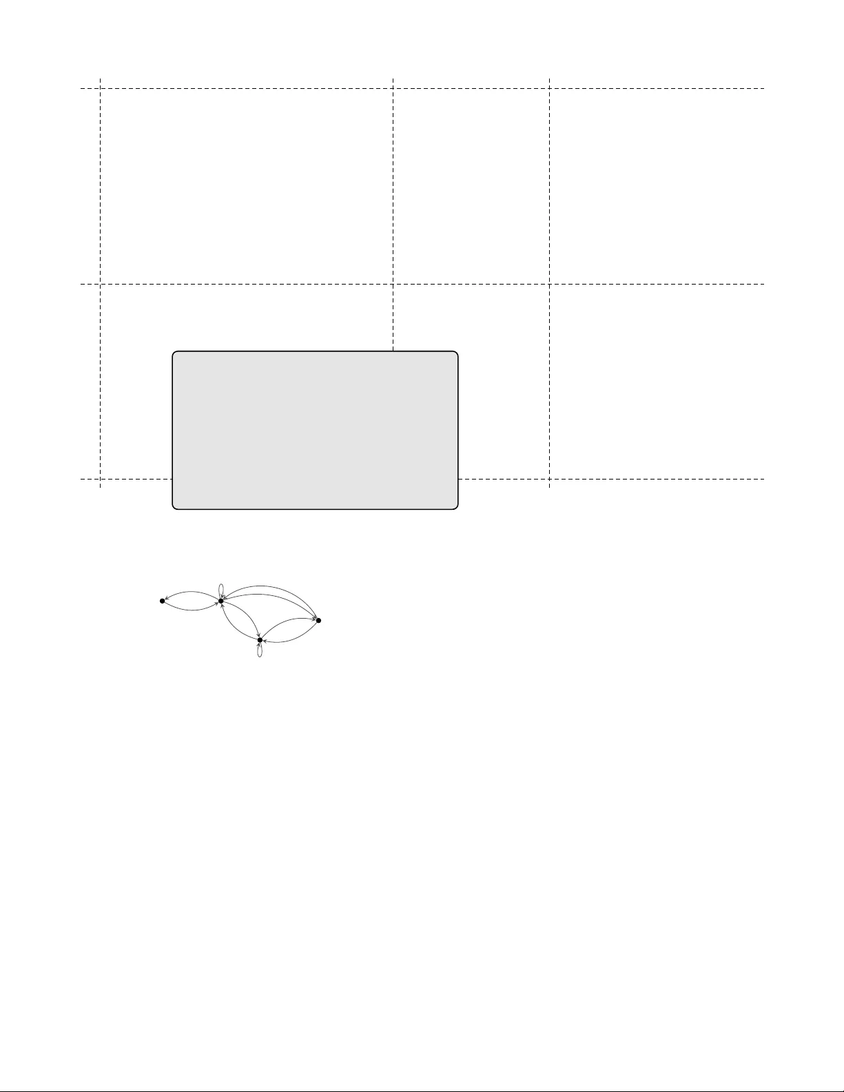
A Controller Synthesis Frame work for W eakly-Hard Control Systems Marc Seidel 1 , Martina Maggio 2 , Frank Allgöwer 1 1 Univ ersity of Stuttg art, Institute for Systems Theory and Automatic Control, Germany 2 Saarland University , Department of Computer Science, Germany & Lund University , Department of Automatic Control, Sweden ©2026 IEEE. Personal use of this material is permitted. Permission from IEEE must be obtained for all other uses, in any current or future media, including reprinting/republishing this material for advertising or promotional purposes, creating new collective works, for resale or redistribution to servers or lists, or reuse of any copyrighted component of this work in other works. Abstract —Deadline misses are mor e common in real-world systems than one may expect. The weakly-hard task model has become a standard abstraction to describe and analyze how often these misses occur , and has been especially used in control applications. Most existing control approaches check whether a controller manages to stabilize the system it controls when its implementation occasionally misses deadlines. However , they usually do not incorporate deadline-overrun knowledge during the controller synthesis process. In this paper , we present a framework that explicitly integrates weakly-hard constraints into the control design. Our method supports various overrun han- dling strategies and guarantees stability and performance under weakly-hard constraints. W e validate the synthesized controllers on a Furuta pendulum, a repr esentative control benchmark. The results show that constraint-aware controllers signiﬁcantly outperform traditional designs, demonstrating the beneﬁts of proacti ve and informed synthesis for overrun-awar e real-time control. I . I N T RO D U C T I O N In real-time control systems, deadline misses are an un- av oidable reality , as conﬁrmed by surveys conducted among industrial practitioners [3], [4]. In fact, occasional timing violations are not only common b ut often tolerated in real systems [14]. Despite the best efforts in scheduling and re- source provisioning, transient ov erloads, computational delays, or communication latencies can lead to tasks missing their deadlines [41]. T o capture the patterns of deadline misses that may occur in real systems, both the industrial and academic communities hav e con verged on the weakly-hard (WH) task model [7], [24]. Rather than requiring strict adherence to e very dead- line, WH models allow a bounded number of misses o ver a ﬁnite sequence of activ ations, typically expressed as the AnyMiss ( r , s ) constraint, meaning that at most r deadline misses may occur in any window of s consecutiv e acti vations. This model offers a realistic abstraction of system behavior via ﬁnite state machines [55], while still enabling formal reasoning about scheduling [59], [61], stability , and control performance [36], [48], [50]. Research on weakly-hard real-time control has largely fo- cused on analysis or synthesis for stabilization. This means checking whether a controller designed for nominal timing conditions remains stable under a given WH execution pat- tern [41], [56] or designing a controller that can stabilize a system under WH packet dropouts [8], [22], [38], [39], [50]. T echniques such as L yapunov functions and the joint spectral radius hav e proven ef fective in establishing guarantees of stability and bounded performance degradation [46], [50], [53]. Howe ver , the synthesis approaches are usually limited to packet dropouts and the analysis approaches typically treat deadline misses as an afterthought: the controller is designed without considering them, and robustness to deadline misses is veriﬁed only afterward. This paper takes a different perspectiv e. W e ask a funda- mental question: What if we know in advance that certain patterns of deadline misses will occur? Can we use this knowl- edge proactiv ely for controller synthesis to achieve better performance and robustness? Our work addresses this open problem by introducing a controller synthesis frame work that explicitly incorporates WH constraints during the controller design phase. T o ground our approach in a meaningful real-world sce- nario, we implement and test our controllers on a Furuta pendulum, a benchmark system that exhibits many of the challenges faced in controller design and has been used as a representativ e control example in recent work [11], [44]. These include intrinsic physical instability , comple x nonlinear dynamics that must be linearized for control, and multiple sensor inputs that must be fused in real time. Our experimental results show that controllers designed with a wareness of WH constraints can signiﬁcantly outperform traditional designs. By accounting for the structure of deadline miss-patterns, we are able to maintain system stability and performance ev en under aggressive timing faults. This high- lights the v alue of shifting from reacti ve analysis to proacti ve (constraint-aware) synthesis in the design of robust real-time control systems. The contribution of this paper is as follows: – A controller synthesis framew ork for control tasks under WH constraints that explicitly supports multiple deadline handling strategies. Our work is inspired by prior work that focuses on packet dropouts in networked control sys- tems [38], [39], [48], but our frame work incorporates the semantics of the deadline handling strategies directly into the controller synthesis phase. This allows the resulting controller to adapt to deadline overruns. – A synthesis method based on switched system representa- tions and linear matrix inequalities. Our method accounts for the structure of WH constraints and generates both non-switching and switching controllers that guarantee stability and performance, both robust with respect to a giv en pattern of deadline misses. The switching controller can adjust its behavior based on recent execution his- tory , impro ving rob ustness to larger numbers of deadline misses. – A comprehensi ve experimental e valuation on a Furuta pendulum, a classic control benchmark. W e demon- strate that constraint-aware controllers designed using our framew ork signiﬁcantly outperform traditional designs in terms of stability and control performance. These results highlight the practical impact of incorporating deadline miss patterns and ov errun semantics into the control design process. The remainder of this paper is organized as follows. Sec- tion II introduces related work. Section III provides back- ground on control theory and WH tasks that are needed in the following sections. Section IV presents the control problems and solutions and Section V shows our experimental ev aluation. W e conclude with Section VI. I I . R E L A T E D W O R K T raditional real-time analysis often assumes that every deadline miss or pack et loss is catastrophic. This assumption is ov erly rigid for many control systems, where occasional faults can be tolerated provided they are suf ﬁciently rare or bounded [7], [10], [17], [52]. T o address this, researchers have introduced more ﬂexible failure models: – Pr obabilistic approaches describe failures as stochastic processes (for example, using Marko v models to rep- resent mode switches between “healthy” and “faulty” operation) providing guarantees in terms of risk rather than absolute bounds [5], [15]–[17], [42]. – Deterministic approaches, such as the WH task model [7], capture bounded sequences of f ailures by e xpressing them as constraints on periodic operations. This model has been successfully applied to control system veriﬁcation [2], [8], [22], [23], [25]–[27], [29], [30], [38], [39], [46], [57], [59], [60] and even adopted in industrial settings [19], [20], [41]. From an analysis and controller synthesis perspectiv e, the closest contributions are related to deterministic models and fault-tolerant systems. The y hav e been inv estigated in theory and moti vated using networked control settings. Ho we ver , the theory of this setting is limited in its applicability to real-time control systems to speciﬁc implementations (namely tasks that are using the Kill overrun strategy , described in Section III), since a packet dropout due to lossy communication equals (in view of the underlying dynamics) a job that is terminated when the deadline is missed. Early work focused on models that bound the maximum number of consecuti ve dropouts, de velop- ing both analysis [51] and controller synthesis techniques [21], [58]. There are also methods for linear systems with data loss under an AnyMiss ( r , s ) for analysis [32], [50] and synthesis [50]. Later , WH constraints have been used to model packet dropouts in networked control settings, generalizing abov e mentioned dropout models. This includes stability analysis [8], [38], [56], also for nonlinear systems [28], [29], and stability and performance-based controller synthesis [18], [36], [38], [39], [48]. From this we conclude that there are sev eral contributions that of fer theoretical guarantees (and synthesis methods), but they all consider simplifying assumptions on the execution in a real-time control setting. In particular , most e xisting ap- proaches to control design for WH systems implicitly assume a kill-task semantics: at a deadline miss, the controller is reset and any partial computation is discarded (e.g., the ap- proaches in [8], [36], [38], [48], [56] and related works). This assumption is con venient because the analysis and synthesis methods dev eloped for packet dropouts can then be directly applied to the deadline miss scenario, but it is not representa- tiv e of typical controller implementations. In fact, common operating systems do not support “kill on ov errun” out of the box. If such semantics are desired, the control engineer must implement them explicitly , e.g., by inserting deadline checks during execution and triggering a self-reset operation when the computation is unsuccessful. While feasible, this is not common practice, and adds non-negligible computational ov erhead, which is undesirable precisely in settings where deadlines are already tight and misses may occur . In many existing systems, it is much more likely that the controller continues executing and performs a time check only at the end of its computation, using that check to decide when to start the next iteration at the next natural activ ation point. This ex ecution semantic corresponds to the Skip strategy (described in Section III) rather than Kill . The approaches mentioned abov e for controller synthesis are therefore not explicitly applicable to cases in which tasks cannot be aborted (or are not aborted), and the controller state is not rolled back at a miss. While some related work considers skipping behavior [19], [20], these approaches typically provide only probabilistic guarantees, and may entail substantial online computational overhead, making it dif ﬁcult to deploy in con- trol tasks with small periods. The challenge of adapting these theoretic results to methods with assumptions that are closer to the controller implementation is so far widely unsolved, and this paper aims at making a contribution in that direction. I I I . B AC K G RO U N D W e consider the discrete-time linear time-inv ariant plant x ( t + 1) = Ax ( t ) + B u a ( t ) + B w w ( t ) z ( t ) = C x ( t ) + D u a ( t ) + D w w ( t ) (1) with time t ∈ N 0 , initial state x 0 : = x (0) ∈ R n , actuator input u a ( t ) ∈ R m , performance input w ( t ) ∈ R q , performance output z ( t ) ∈ R p , and system matrices of appropriate dimen- sions with real-number entries. The objectiv e of this work is to design a control law and implement it in a control task T . Said task executes according to the Logical Execution T ime paradigm [35], and hence the corresponding control la w should consider that the controller implementation introduces a 1-step delay [12]. T o that end, we introduce the delayed plant model  x ( t + 1) u ( t + 1)  =  A B 0 0  x ( t ) u ( t )  +  0 I  u a ( t ) +  B w 0  w ( t ) z ( t ) =  C D   x ( t ) u ( t )  + 0 · u a ( t ) + D w w ( t ) (2) with the augmented state u ( t ) = u a ( t − 1) ∈ R m and some initial value u (0) . Here, I and 0 denote the identity and zero matrix of suitable dimension, respectiv ely . The control task computes stateless state-feedback controllers of the form u c ( t ) = K  x ( t ) ⊤ u ( t ) ⊤  ⊤ , (3) with the computed control input u c ( t ) ∈ R m and the controller gain matrix K ∈ R m × n . Note that the inherent one-step delay is already contained in the delayed plant model (2). Further , note the dif ference between the applied input u a ( t ) and the computed input u c ( t ) . In the next subsection we discuss how u a ( t ) and u c ( t ) relate to one another . A. Modeling the Effects of Deadline Misses Under nominal conditions, all acti vated jobs of the control task T ﬁnish before their deadlines. Then, the applied control signal u a ( t ) equals the computed control signal u c ( t ) , i.e., u a ( t ) = u c ( t ) . Hence, the controller (3) may directly inﬂuence the (delayed) plant at any time t . 1 Howe ver , some control tasks’ jobs may miss their deadline. Thus, u a ( t ) and u c ( t ) are not always equal. T o describe deadline misses formally , we introduce the binary hit/miss sequence µ : = ( µ ( t )) t ∈ N 0 , where µ ( t ) = 0 in case of a deadline miss and µ ( t ) = 1 for a deadline hit. For the purpose of this hit/miss sequence, we interpret a “recovery hit” (i.e., the hit of a job that missed at least one previous deadline and was allowed to continue ex ecuting) as a hit. This means that µ ( t ) encodes whether a control job has completed its execution during the t -th period. W ithout loss of generality , we assume µ (0) = 1 , i.e,. the very ﬁrst job of the control task completes before its deadline. T wo immediate questions arise whene ver a deadline miss occurs: (i) how to set the next control input and (ii) what to do with the control job that e xhibited the computational overrun. W e use the term actuator strate gy to refer to the answer to (i) and overrun strate gy to refer to the answer to (ii). T wo commonly used actuator strategies are Zer o and Hold . For Zer o , the next control input is simply set to zero, while for Hold the pre vious input is held until a new control input is av ailable. Formally , we can write u a ( t ) = ( µ ( t ) u c ( t ) Zer o µ ( t ) u c ( t ) + (1 − µ ( t )) u a ( t − 1) Hold (4) Which of those actuator strategies is more advantageous depends heavily on the control system [47]. Therefore, both actuator strategies are practically rele vant. 1 Note that this corresponds to the logical ex ecution time paradigm appli- cation, due to the delay being applied at the plant lev el. The literature considers mainly three o verrun strate gies: Kill , Skip , and Queue [13], [41], [45]. F or Kill , the job is killed at its deadline and a ne w one is started, effecti vely omitting all computations of the killed job . The Skip strategy on the other hand allows the job to continue after it missed its deadline and skips the next job entirely . This allows the job to ﬁnish. In case the next job is not skipped b ut queued instead, i.e., as soon as the ﬁrst job ﬁnishes, the queued one starts immediately , the Queue strategy emerges. Note that in principle it is possible to queue multiple jobs, but in light of control tasks and stateless controllers it is only reasonable to queue at most one job, referring to as Queue (1) . Queuing more than one job would inherently use old state information, which is disadv antageous for the control goals. Thus, for stateless control jobs, typically only Queue (1) is considered [13], [45]. Recently , Queue has been empirically sho wn to be beneﬁ- cial [11]. Howe ver , the ability to provide formal guarantees when using Queue is impaired by the presence of different alternativ es after a job ov erruns: The original job could not ﬁnish, it could ﬁnish but the queued one could not, or it ﬁnished and a fresh job also completes its execution. This makes the outcome nondeterministic [41], hence harder for controller synthesis purposes. As we want formal arguments, in this paper, we focus on Kill and Skip only . 2 B. Modeling the Occurr ence of Deadline Misses In many practical implementations, factors such as ov erload are causing deadline misses. These factors are typically known in the system but external to the control pipeline, making their occurrence to some extent predictable. The automoti ve industry has de facto adopted the WH task model [1], [20], [25], [27], [41] to describe the occurrence of deadline misses, that constrains the permissible number of deadline misses within a speciﬁc time windo w . Deﬁnition 1 (WH constraint: AnyMiss ) . A contr ol task T satisﬁes the WH constraint λ = AnyMiss ( r, s ) , denoted by T ⊢ λ , if in any s consecutive job activations of T , at most r of them miss their deadline. For a more detailed description and other types of WH constraints, such as AnyHit , RowHit , and RowMiss , we refer to the seminal paper [7]. The frame work presented in this paper is similarly applicable to other kno wn types of WH constraints. W ith a slight abuse of notation, we also write µ ⊢ λ whenever the hit/miss sequence µ associated with T satisﬁes the WH constraint λ . W e are now ready to formally deﬁne our considered system class, namely the class of WH control systems , as follows. Deﬁnition 2 (WH control system) . A WH contr ol system is the plant (1) contr olled by the contr ol task T satisfying the WH constraint λ and computing the contr oller (3) and either 2 The paper makes two contributions: analysis and design. It is in principle possible to analyze the Queue (1) strategy with our proposed frame work, similarly to the analysis proposed in [41], but the control design prov es to be signiﬁcantly more challenging. This is due to the more in volv ed dynamics that are required to adequately model the ov erall system under Queue (1) . Zero or Hold as actuator strate gy , and Kill or Skip as overrun strate gy . The synthesis of controllers for WH control systems is the main topic of the paper at hand. One of our control goals, apart from stability , is to synthesize controllers with guaranteed performance. The considered performance metric is introduced in the subsequent subsection. C. Contr ol System P erformance When e valuating a system’ s behavior , merely considering stability is typically not suf ﬁcient. Rather , performance metrics are used to quantify ho w well a system beha ves. For WH control systems, a common metric is found in quadratic stage costs or LQR-like measures, see, e.g., [50], [53]. In this paper , we consider a different performance measure, commonly known as ℓ 2 -performance [34]. For that, the perfor- mance input w and performance output z from Equations (1) and (2) are used. Thereby , w → z is called the performance channel . The signal w represents factors and inﬂuences on the system that are typically undesired, but cannot be av oided, such as disturbances. On the other hand, z contains quantities that are of interest for the control objectiv e, for example weighted costs in x , measuring deviation from a desired operating point. In its essence, ℓ 2 -performance measures the inﬂuence of w on z , considered in a quadratic fashion. When designing controllers that improv e the ℓ 2 -performance, one aims at reducing the inﬂuence of the unwanted factors on the relev ant quantities. Thus, ℓ 2 -performance quantiﬁes how large the output z will be if we know ho w large the input w is. W e formally deﬁne ℓ 2 -performance for WH control systems as follows. Deﬁnition 3 ( ℓ 2 -performance for WH control systems) . De- note the set of all squar e-summable signals ℓ 2 = { w | P ∞ t =0 w ( t ) ⊤ w ( t ) < ∞} . The WH control system is said to have ℓ 2 -performance with gain γ < ∞ if it is asymptotically stable, and for x 0 = 0 it holds that ∞ X t =0 z ( t ) ⊤ z ( t ) < γ 2 ∞ X t =0 w ( t ) ⊤ w ( t ) ∀ w ∈ ℓ 2 , w  = 0 , ∀ µ ⊢ λ . (5) Note that this includes asymptotic stability , i.e., whenev er a WH control system has a guaranteed ℓ 2 -performance gain γ < ∞ it is also guaranteed to be asymptotically stable. In many engineering applications, physically rele vant quan- tities naturally appear as energy-like terms. The summation ov er all squared w ( t ) , resp. z ( t ) , in (5) is often able to represent such terms, making the considered performance mea- sure applicable to a lar ge class of practically relev ant control systems. Consequently , the set ℓ 2 can be interpreted as all signals w with ﬁnite ener gy . Since Deﬁnition 3 considers one γ for all possible w , c.f. (5), ℓ 2 -performance can be practically interpreted as the worst-case ener gy ampliﬁcation through the performance channel. The smallest γ such that (5) is still satisﬁed is called the ℓ 2 -gain of the system. Any γ satisfying (5) thus constitutes an upper bound on the inﬂuence (or energy ampliﬁcation) from w to z . That means, loosely speaking, γ quantiﬁes by ho w much w is ampliﬁed (or attenuated) by the system. As a consequence, a small γ indicates a good performance, since undesired factors hav e small inﬂuence on relev ant quantities z , while a large γ means that w can hav e a larger inﬂuence on z . Note that the signals w and z , as well as the related matrices B w , C , D , and D w , can in practice often be chosen or tuned in a suitable manner , as they are typically artiﬁcial. For example, by altering C and D one can tune how relev ant a state or an input is for the overall behavior of the control system. Or it might be unknown how exactly a disturbance affects the system, but from an engineering viewpoint it might be clear that it affects one state more than another . In this case, B w can be chosen suitably to reﬂect this inﬂuence. As a consequence, the considered performance measure is more ﬂexible in practice than one might think. W e provide reasoning for choosing the performance channel based on the desired behavior of a real-w orld example in our e xperimental ev aluation in Section V. I V . C O N T R O L L E R S Y N T H E S I S This section introduces our control design frame work. Its main purpose is the design of controllers with theoretical performance guarantees for WH control systems. Ho we ver , our framew ork also allo ws us to analyze WH control systems un- der existing controllers for their stability and/or performance. In summary , we aim to provide solutions to the follo wing three different analysis and synthesis problems for ℓ 2 -performance of WH control systems. Problem 1. Analyze a given WH contr ol system with a given contr oller for its guaranteed ℓ 2 -performance. Problem 2. Given a WH contr ol system, ﬁnd a non-switching contr oller that achie ves the best guaranteed ℓ 2 -performance. Problem 3. Given a WH control system, ﬁnd a switching contr oller that achie ves the best guaranteed ℓ 2 -performance. Problem 1 constitutes an analysis problem. On the other hand, Problems 2 and 3 deal with the synthesis of WH control systems with guaranteed ℓ 2 -performance. The subtle yet crucial difference between Problem 2 and 3 is whether the controller matrix K may be switching (i.e., be different for different controller jobs) or non-switching. W e explain the functionality of a switching controller, the dif ference between switching and non-switching controllers, and their inﬂuence on the design procedure in Subsection IV -D. A. The frame work The workﬂow of the proposed frame work 3 for synthesizing controllers in volv es three different components: 1) Computing a suitable system representation, 2) Computing the WH graph, 3) Solving a linear matrix inequality optimization problem. 3 Functional M A T L A B-code for designing controllers using this framework is available at https://gitlab.cs.uni- saarland.de/rtsc/gss . Solve LMI problem Compute WH graph Compute system representation Switched system (8) WH graph G (Section IV -C) Controller K with guaranteed performance γ Design choice: non-switching or switching controller WH constraint λ System Matrices: matrices A , B P erformance channel: matrices B w , D w , C , D Implementation choices: Hold or Zer o Kill or Skip Fig. 1. W orkﬂow of the proposed controller design frame work. An ov erview of the dif ferent components, their interplay , and how the dif ferent aspects of the WH control system and design choices of the control task inﬂuence the w orkﬂo w is depicted in Figure 1. In 1), the plant model is to be put into an adequate system representation. T o compute this representation, the performance channel and controller implementation have to be chosen. The result is a so-called switched system [37], a system class that is widely used and in vestigated and which we introduce in Subsection IV -B. In parallel, the representation of the WH constraint as a graph, the so-called WH graph , can be computed for 2). T ogether with controller design choices, a well-behav ed con ve x optimization problem is solved as a last step. The output is a deadline miss-a ware controller with a guaranteed performance lev el. In case the result is not satisfactory , one or more of the inputs to the procedure can be altered. The inv olved components then need to be recomputed. B. System r epresentation The goal of this subsection is to formulate the WH control system as a mathematical model kno wn as switched system . Switched systems are piecewise linear systems that at each time step may admit different dynamics. Its general form in closed-loop is ˜ x ( ˜ t + 1) = A cl σ ( ˜ t ) ˜ x ( ˜ t ) + B w σ ( ˜ t ) ˜ w ( ˜ t ) ˜ z ( ˜ t ) = C cl σ ( ˜ t ) ˜ x ( ˜ t ) + D w σ ( ˜ t ) ˜ w ( ˜ t ) , (6) where the switched system matrices denoted by calli- graphic letters may switch in each time step ˜ t between a ﬁnite set of matrices, i.e., ( A cl σ ( ˜ t ) , B w σ ( ˜ t ) , C cl σ ( ˜ t ) , D w σ ( ˜ t ) ) ∈ { ( A cl l , B w l , C cl l , D w l ) | l = 1 , . . . , L < ∞} for all ˜ t . The variable l is called mode of the switched system and de- notes which set of system matrices is currently activ e, and σ ( ˜ t ) ∈ { 1 , . . . , L } is called the switching signal . T o reformulate the WH control system given actuator and ov errun strategies as a switched system of the form (6), it is helpful to consider only time instants at which state t µ = H/R 1 M 0 M 0 H/R 1 H/R 1 M 0 H/R 1 τ Kill = 0 3 4 6 τ Skip = 1 4 5 7 α = 2 0 1 Fig. 2. Example sequences, denoting M, H, R for a miss, hit, or reco very hit, respectively . measurements actually inﬂuence the plant through the con- troller via (3). Due to deadline misses, at some time instants the controller does not inﬂuence the plant and the system essentially runs open-loop. In the context of the Kill strategy , considering only the inﬂuential time points was pre viously called lifting [48] or alternative discr etization [38]. First, consider the Kill strategy . Since killing a job essen- tially deletes the state information that the job was started with, only state information at time instants where a deadline hit occurs are rele v ant for control input actuation. Therefore, we only consider time points where µ ( t ) = 1 . Formally , we deﬁne τ Kill = { t | µ ( t ) = 1 } as the set of relev ant time instants. Denote with τ Kill ( ˜ t ) the ˜ t -th element of τ Kill in ascending order . For the Skip strategy , on the contrary , the job that was started after a hit (or recov ery hit) continues until completion. All following job acti v ations are skipped and the corresponding state measurements are irrelev ant for control input computa- tion. Thus, the state information at time instants after a hit (or recov ery hit) are relev ant for control input actuation. As a consequence, we hav e τ Skip = { t | µ ( t − 1) = 1 } as the set of rele vant time instants for the Skip strate gy . F or ease of presentation, we use τ as shorthand notation for either τ Kill or τ Skip . Next, for ease of notation, we introduce the sequence α that counts the number of consecutiv e deadline misses between hits or recoveries, similar to [38], [48]. Since µ ⊢ λ = AnyMiss ( r, s ) , the elements of α are within the set Σ : = { 0 , . . . , r } , where r is the maximum number of con- secutiv e deadline misses. Further , the sequences µ and α provide equi v alent representations of the deadline misses and hits/recov eries, i.e., α ⊢ λ ⇐ ⇒ µ ⊢ λ . The different sequences and time instant sets τ are vi- sualized by the following example and the corresponding Figure 2. Consider the hit/miss sequence µ = (1 0 0 1 1 0 1 . . . ) starting at time t = 0 . It follows that for this speciﬁc µ , τ Kill = (0 3 4 6 . . . ) and τ Skip = (1 4 5 7 . . . ) . The correspond- ing sequence of consecuti ve misses is α = (2 0 1 . . . ) . W e are now ready reformulate the WH control system as a switched system of the form (6). First, we set ˜ x = [ x ⊤ u ⊤ ] ⊤ ∈ R n + m , as we use the delayed plant model in Equation (2). Furthermore, since the τ -sets are directly linked to time instants with hits or recovery hits, the dynamics be- tween τ ( ˜ t ) and τ ( ˜ t + 1) depend on the corresponding value of α ( ˜ t ) , as this sequence indicates the number of misses between τ ( ˜ t ) and τ ( ˜ t + 1) . Consequently , the modes of the switched system are deﬁned by σ ( ˜ t ) = α ( ˜ t ) ∈ Σ and correspond to the number of consecutive deadline misses between τ ( ˜ t ) and τ ( ˜ t + 1) . Thus, α acts as the switching sequence for (6). Since for ℓ 2 -performance, w ( t ) and z ( t ) for all t need to be considered, c.f. (5), it is not sufﬁcient to merely take w ( τ ( ˜ t )) and z ( τ ( ˜ t )) into account. W e therefore need to stack the performance input and output signals between those time instants, as in [48]: ˜ w ( ˜ t ) =    w ( τ ( ˜ t − 1)) . . . w ( τ ( ˜ t ) − 1)    , ˜ z ( ˜ t ) =    z ( τ ( ˜ t − 1)) . . . z ( τ ( ˜ t ) − 1)    . (7) W e then arri ve at the switched system form (6), reading as  x ( ˜ t + 1) u ( ˜ t + 1)  = ( A α ( ˜ t ) + B α ( ˜ t ) K )  x ( ˜ t ) u ( ˜ t )  + B w α ( ˜ t ) ˜ w ( ˜ t ) ˜ z ( ˜ t ) = ( C α ( ˜ t ) + D α ( ˜ t ) K )  x ( ˜ t ) u ( ˜ t )  + D w α ( ˜ t ) ˜ w ( ˜ t ) . (8) Note that due to the considerations of time instants τ ( ˜ t ) only , one time step of the switched system (8) may correspond to multiple time instants of the original plant (1). The matrices A α ( ˜ t ) , B α ( ˜ t ) , B w α ( ˜ t ) , C α ( ˜ t ) , D α ( ˜ t ) , and D w α ( ˜ t ) depend on the chosen actuator and overrun strategies. Through algebraic computation of the dynamics from time τ ( ˜ t ) to τ ( ˜ t + 1) , i.e., from one time instant that inﬂuences the system through the controller to the next one, one obtains the switched system matrices shown in Figure 3 for (8). In summary , the switched system as a result of the frame- work’ s component 1) can be obtained by computing the matrices in Figure 3 for the respectiv e actuator and overrun strategies. The system representation of the WH control system is then given by the switched system (8). Recall that the switching of (8) admits to the WH constraint. As a next step, we aim to represent the WH constraint by a graph that generates the permissible switching signals, constituting component 2) of the frame work. C. W eakly-har d graph In the previous subsection, we reformulated the WH control system as a switched system with the switching signal α . Even though there is vast literature on switched systems with arbitrary switching, i.e., no restrictions on α , the switching of (8) is in fact restricted due to the WH control system admitting to the WH constraint. The WH constraint limits the possible hit/miss combinations and therefore imposes a switching rule on α . In the literature, it has been prov en useful to represent the WH constraint by a graph, see, e.g., [8], [24], [38], [48], [55]. In the subsequent deﬁnition, we introduce the WH graph , but refer to the cited literature for details. Deﬁnition 4 (WH graph) . Consider the directed graph G = ( V , E ) , wher e V is the set of all nodes v i , i = 1 , . . . , n V , and E denotes the set of edges e k , k = 1 , . . . , n E , where e k = ( i, j, l ) ∈ E if there exists an edge fr om node v i to node v j with label l . G is a WH graph for the WH contr ol system if the langua ge of G is equivalent to the set of all α -sequences with α ⊢ λ . All permissible hit/miss sequences satisfying the WH con- straint can thus be encoded by moving along the edges of G . Also, all sequences α that correspond to a path on G are permissible hit/miss sequences, i.e., α ⊢ λ . Consequently , all sequences generated by G constitute possible switches between the modes α ( ˜ t ) of the switched system (8). Figure 4 shows G for the example of an AnyMiss (3 , 5) constraint. Note that Deﬁnition 4 is equal to the notion of the lifted graph from [48] or [38], which differs slightly from earlier notions [24], [55]. The basic principle howe ver is the same. The generation of such a graph is alw ays possible and cor- responding algorithms are av ailable [39], [55]. This is also possible for the other types of WH constraints [7], [56], which in turn means that our frame work is applicable for all WH constraints. D. Solve optimization pr oblem Using the system representation from Subsection IV -B and the WH graph as e xplained in Subsection IV -C, we can now solve Problems 1–3. The solution of those problems in volv es solving an op- timization problem containing Linear Matrix Inequalities (LMIs). LMIs are naturally semideﬁnite programs and thus con vex. They are well understood and widely used in linear control theory [9] and there are powerful tools [40], [43] for various programming languages for solving problems inv olv- ing LMIs. As a consequence, LMI problems can be solved reliably and efﬁciently . The LMI problems appearing in the context at hand take the form min δ γ such that M ≻ 0 , (9) where M = { M 1 , M 2 , . . . } is a set of real symmetric matrices that individually shall satisfy M k ≻ 0 for all k and δ are the decision variables (speciﬁed later separately for each problem). The solution of this conv ex optimization problem is the achie ved ℓ 2 -performance gain γ and, in case of synthesis, the optimal controller K computed from the optimal v alues of the decision v ariables δ . W e now specify M and δ for each of the Problems 1– 3 by reformulating them into the form (9). In all of them, the matrix set is M = { M k | e k = ( i, j, l ) ∈ E } , i.e., it contains n E matrices M k , that pose a condition on each edge e k of the WH graph G = ( V , E ) . Further , the set of decision variables contains graph-global decision v ariables δ G and a set of node-dependent decision variables δ i for each v i ∈ V , i.e., δ = S v i ∈V δ i ∪ δ G . For Kill , [48] reports how the resulting LMI problems guarantee ℓ 2 -performance. Here, we additionally extend this to Skip by pro viding the respectiv e switched system matrices in Figure 3, making it a broadly applicable frame work. Subsequently , we state the three optimization problems in volving LMI problems to provide the solution for our original research Problems 1–3 in order . Kill Skip Common Zero Hold A α =  A α +1 A α B 0 0  , B α =0 =  0 I  C α =0 =  C D  , D α =0 = 0 C α ≥ 1 =      C A 0 D C A 1 C A 0 B . . . . . . C A α C A α − 1 B      , D α =1 =  0 D  B α ≥ 1 =  A α − 1 B 0  D α ≥ 2 =        0 D C A 0 B . . . C A α − 2 B        B α ≥ 1 =   α − 1 P i =0 A i B I   D α ≥ 2 =          0 D D + C B . . . D + C α − 2 P i =0 A i B          B α =  0 I  , D α = 0 A α and C α : same as Kill, Common A α =   A α +1 α P i =0 A i B 0 0   C α =0 =  C D  C α ≥ 1 =        C A 0 D C A 1 D + C B . . . . . . C A α D + C α − 1 P i =0 A i B        For all strategy combinations: B w α =  A α B w . . . A 0 B w 0 . . . 0  , D w α =0 = D w D w α ≥ 1 =       D w 0 · · · 0 C A 0 B w · · · · · · · · . . . . . . · · · · · · · · · · 0 C A α − 1 B w · · · C A 0 B w D w       Fig. 3. Switched system matrices for different actuator and overrun strategy combinations, omitting the time argument of α ( ˜ t ) for conciseness of notation. · · · · α = 3 0 1 0 2 0 2 1 1 0 Fig. 4. Example of a WH graph G for the AnyMiss (3 , 5) constraint. Optimization Problem 1 (Analysis) . The analysis Problem 1 is solved by the LMI pr oblem (9) with δ G = { γ } , wher e γ ∈ R , and δ i = { S i , G i } , wher e S i ∈ R ( n + m ) × ( n + m ) symmetric, G i ∈ R ( n + m ) × ( n + m ) , i = 1 , ..., n V , and M = { M k | e k = ( i, j, l ) ∈ E } with M k =     G i + G ⊤ i − S i ∗ ∗ ∗ ( A l + B l K ) G i S j ∗ ∗ 0 ( B w l ) ⊤ γ I ∗ ( C l + D l K ) G i 0 D w l γ I     , (10) wher e ∗ denote matrix blocks than result fr om the symmetry constraint. The theoretical guarantee can be obtained by similar argu- ments as in [48, Theorem 2] using an equivalent congruence transformation of the in volv ed LMIs and leading to a node- dependent L yapunov function characterized by the S i ’ s. For controller synthesis, we obtain the following results. Optimization Problem 2 (Non-switching controller synthe- sis) . The non-switching contr oller synthesis Problem 2 is solved by the LMI pr oblem (9) with δ G = { G, R, γ } , where γ ∈ R , G ∈ R ( n + m ) × ( n + m ) , R ∈ R m × ( n + m ) , and δ i = { S i } , wher e S i ∈ R ( n + m ) × ( n + m ) symmetric, i = 1 , ..., n V , and M = { M k | e k = ( i, j, l ) ∈ E } with M k =     G + G ⊤ − S i ∗ ∗ ∗ A l G + B l R S j ∗ ∗ 0 ( B w l ) ⊤ γ I ∗ C l G + D l R 0 D w l γ I     . (11) The non-switching controller is computed fr om the solution of LMI pr oblem (9) by K = RG − 1 . Note that Optimization Problem 2 giv es us the best possible controller K that guarantees the performance lev el γ under any permissible hit/miss sequence. Ho wever , the solution K is then independent of the hit/miss sequence. It is adv antageous to let the controller gain matrix adapt to the current operating conditions, i.e., the currently experienced hit/miss pattern. This is achie ved by synthesizing one separate gain matrix K i per node v i of the WH graph. Then, the applied controller is u c ( t ) = K i x ( t ) and depends on the current node of the WH graph, thus implicitly depending on the past hit/miss pattern. This typically increases the feasibility of the approach and improv es the achiev ed performance guarantee. The subsequent optimization problem states the corresponding LMIs for switching controller synthesis. Optimization Problem 3 (Switching controller synthesis) . The switching controller synthesis Pr oblem 3 is solved by the LMI problem (9) with δ G = { γ } , where γ ∈ R , and δ i = { S i , G i , R i } , where S i ∈ R ( n + m ) × ( n + m ) symmetric, G i ∈ R ( n + m ) × ( n + m ) , R i ∈ R m × ( n + m ) , i = 1 , ..., n V , and M = { M k | e k = ( i, j, l ) ∈ E } with M k =     G i + G ⊤ i − S i ∗ ∗ ∗ A l G i + B l R i S j ∗ ∗ 0 ( B w l ) ⊤ γ I ∗ C l G i + D l R i 0 D w l γ I     . (12) The switching contr oller is computed from the solution of LMI pr oblem (9) by K i = R i G − 1 i for each node v i ∈ V . Finally , it is worth mentioning that one can adapt the LMIs to neglect performance and focus on stability only . The result is either an analogous analysis procedure for asymptotic stability in the case of (10), or the synthesis of a stabilizing controller without any performance considerations for (11) and (12). T o do so, only consider the upper left 2-by-2 block of the matrices M k in (10), (11), or (12). Then, the LMIs collapse to the ones deri ved in the conte xt of network ed control systems under WH transmission dropout descriptions in [38]. Recall though that asymptotic stability is implicitly included in the deﬁnition of ℓ 2 -performance and therefore the resulting controllers will also asymptotically stabilize the WH control system. E. Discussion First, we want to stress that our method explicitly takes deadline misses into account, i.e., it allo ws us to design controllers speciﬁcally for a certain WH constraint. Next, note that upon changes, the framework only requires to recalculate the necessary parts. F or example, when changing from Kill to Skip one only needs to recompute the system representation, but not the WH graph, as seen in Figure 1. Note that any obtained performance guarantee transfers to other WH control systems with a harder WH constraint [7], [54]. In fact, our framew ork is not limited to WH constraints: it can be used for any graph-based deadline miss model, i.e., for any regular language description of the admissible hit/miss pattern. Observe that our framework is based on the concept of multiple L yapunov functions , that is kno wn to typically provide sufﬁcient conditions only . Consequently , the guarantees pro- vided by our controller design framework are only sufﬁcient as well. Hence, if the optimization problem has no solution, we cannot guarantee stability . Ho wev er, there still might exist a controller that stabilizes the system. T aking a practical approach, one can solve the problem using a harder WH constraint and use the resulting controller, enforcing the harder constraint at the platform le vel. The WH graph can grow large, especially for increasing window lengths s , which imply that man y hit/miss combina- tions are possible. This is essentially the trade-of f for designing a controller that e xplicitly considers all admissible hit/miss combinations. The reduction of the computational b urden that comes with increasing graph size is subject to future work. Note howe ver , that our presented procedure is an ofﬂine design, i.e., none of the frame work’ s components are required to be computed during runtime. This enables the controller design for larger WH graphs, since no problem of the form (9) needs to be posed and solved online. Moreov er , note that the presented approach is able to synthe- size switching stateless state-feedback controllers. Those are more powerful than classical static state-feedback controllers, because they may additionally depend on the last applied input u according to the delayed model (2). The last applied input is easily known to the control task T and grants additional ﬂexi- bility to the controller design. Additionally , using a switching controller K i allows the controller to adapt to past hit/miss patterns and implicitly to future possible ev olutions thereof. This can be interpreted as an adapti ve control task and leads to increased feasibility and performance. The presented framew ork can be used to quantify by how much the guaranteed performance changes if the WH control system admits to a weaker or harder WH constraint instead. This can be used to free computational resources if for example a certain performance guarantee can also be achie ved with a different WH constraint that allows more deadline misses. Related, one can also use the procedure of [31] to ﬁnd all WH constraints for which stability or a certain ℓ 2 - performance lev el γ is guaranteed. The computational complexity and required memory both depend on the size of the WH graph. In the following, we deriv e the number of nodes n V and edges n E of G = ( V , E ) for an AnyMiss constraint. Note that AnyHit and RowMiss constraints can be equiv alently reformulated into an AnyMiss constraint [54]. For space reasons, we also refer to [54] for determining the graph size of RowHit constraints. Determining the graph size is a matter of combinatorics. The nodes of the WH graph encode the admissible combinations of misses and hits/reco veries of the hit/miss pattern µ within the past window of length s . W e ﬁrst aim to ﬁnd the number of edges with a speciﬁc label 0 ≤ l ≤ r , denoted n E ( l ) , corresponding to the α sequence. Recall that an edge with label l corresponds to a hit/miss sequence of length l + 1 with l misses and one hit/recovery , c.f., Section IV -B. Thus, we want to ﬁnd the number of combinations of placing the remaining r − l misses within the preceding s − ( l + 1) time steps. Thus, we ha ve n E ( l ) =  s − 1 − l r − l  , where  · ·  denotes the binomial coefﬁcient. Hence, using Pascal’ s identity , the total number of edges is n E = r X l =0 n E ( l ) = r X l =0  s − l r − l  −  s − l − 1 r − l − 1  =  s r  . (13) The number of nodes arises directly from the fact that e very node can be left with α = 0 and hence is equal to the number of edges with label 0 , i.e., n V = n E (0) =  s − 1 r  . Note that the obtained graph size is smaller than the one presented in [55], as the graph deﬁnitions differ and the lifting implicitly reduces the number of combinations to encode. On the topic of computational comple xity of the optimiza- tion problems, let us denote the number of scalar decision variables with | δ | and the number of constraints with |M| . In the worst case, such a problem is O ( | δ | 3 ln | δ | ) in the decision variables and O ( |M| 1 . 5 ln |M| ) in the number of constraints [6]. Ho wev er, note that the optimization problems at hand hav e similarities to classical L yapunov LMIs, which hav e been reported to be solved signiﬁcantly faster than the worst case, see [9, Section 2.4.4]. The number of decision variables depends both on the state dimension of the delayed plant (2) n + m and on n V . More precisely , for the computationally most demanding Optimization Problem 3, | δ | = n V  ( n + m )( n + m + 1) / 2 | {z } S i + ( n + m )( n + m ) | {z } G i + m ( m + n ) | {z } R i  + 1 |{z} γ . (14) The number of constraints is exactly the number of edges of the WH graph, i.e., |M| = n E . The code size of the designed controller depends on whether the controller is switching or non-switching. Speciﬁcally , the switching controller requires the storage of ( n + m ) gains (dimension of delayed plan model (2)) per component of the control signal u and per node of the graph. This totals to n V · ( n + m ) · m coefﬁcients (ﬂoating points or ﬁxed point values). Space is a reason why the non-switching controller may be preferable in some cases, e.g., on memory-constrained systems, ev en though the switching controller theoretically guarantees better performance. This is also clearly visible in practice. F . Extensions to the frame work W ith a few adaptations, the presented frame work is ﬂexible and can be used for more applications. For example, e ven though the framework includes only stateless controllers with gain matrices K or K i , it can also be used to analyze dynamic controllers. Dynamic controllers are often in vestigated in many related works, for example [53]. As long as one can ﬁnd a closed-loop switched system representation (8), Optimization Problem 1 can be used for ℓ 2 -performance analysis. Synthesizing dynamic or output- feedback controllers ho we ver is signiﬁcantly more challenging and open for future research. In this paper, we consider ℓ 2 -performance, a performance metric very commonly used in practice. Adapting the LMIs to be solved enables to tackle also other performance metrics, such as quadratic performance [36]. It is further possible to include robustness against uncertainties [36]. For plants with state interactions that are constrained by an underlying Fig. 5. The Furuta pendulum used for experimental ev aluation. cone, e.g., widely used positive systems, dif ferent performance metrics can be analyzed. In the case of positiv e systems, the LMIs reduce to linear programs. Thus, our framework can cope with a broader class of systems. F or details thereon we refer to [49]. V . E X P E R I M E N TA L E V A L UAT I ON In this section, we present the results of the experimental ev aluation conducted on a small Furuta pendulum, 4 depicted in Figure 5. Section V -A presents the experimental setup and the performance metrics used for the comparison. Sec- tions V -B and V -C present two experimental setups, comparing controllers designed respecti vely for the Kill and Zer o and the Kill and Hold policy . Sections V -D and V -E present the remaining two e xperimental setups, comparing controllers designed respectiv ely for the Skip and Zer o and the Skip and Hold policy . A. Experimental Setup The control task executes periodically every 5 ms , with activ ations at times a ( t ) , where t counts the job executions. At time a ( t ) , the controller task applies the control signal u ( t ) that has been calculated during the previous period, i.e., the torque applied at the base le vel. It then proceeds to read data from the pendulum sensors: the pendulum angle θ ( t ) , the pendulum angular velocity ˙ θ ( t ) , and the base velocity ˙ ρ ( t ) . The controller is also a ware of its own computational state, i.e., of the sequence ( µ i ) i ∈{ t − s +1 ,...,t − 1 } , that is the hit/miss sequences over the past window of length s . The controller has three operational modes: (i) initialization, (ii) swing up mode, (iii) linear mode. The initialization only lasts for a single iteration, in which the pendulum is forced to mov e by applying a small torque at the base. The swing up mode is then designed to let the pendulum reach the proximity of the upright position (we do not inject deadline misses during the swing up phase, because this would make our experiments not comparable). Finally , the controller operates in linear mode. In this mode we inject deadline misses whose patterns satisfy a WH constraint. Note that – in principle 4 W e use a pendulum built according to the instructions pro vided in the Furuta pendulum posts of https://build-its- inprogress.blogspot.com. – each experiment tests a different randomized pattern. If a deadline miss can occur , depending on what happened during the window , we introduce it with a certain probability . When the probability is 1 . 0 , the experiments and the e xecutions still differ due to the pendulum state in which the ﬁrst deadline miss is injected. The remaining subsections sho w dif ferent experimental se- tups that allow us to compare sev eral controllers. For each experimental setup and each controller , we report statistics on the execution of 100 experiments 5 . For each experiment, we generate a sequence of deadline misses ( µ i ) i ∈{ 1 ,..., 25000 } that satisﬁes a WH constraint AnyMiss ( r, s ) . For the generation, we use the v alue P miss to indicate the probability of missing a deadline when possible. This sequence corresponds to roughly 2 minutes of execution of the controller code (speciﬁcally 125 seconds; the ﬁrst 5 seconds are considered necessary for initialization and swing up to complete, and are discounted from the performance calculation). W e compare our controllers with two baseline alternativ es. The ﬁrst one is the original controller presented in [33], and the second one is a linear quadratic regulator lqr presented in [44]. These are deﬁned by original : u c = 0 . 3750 θ + 0 . 0250 ˙ θ + 0 . 0125 ˙ ρ (15) lqr : u c = 0 . 4280 θ + 0 . 0307 ˙ θ + 0 . 0119 ˙ ρ. (16) For each experimental setup we design the non-switching and switching controllers from Section IV using the pen- dulum model introduced in [44] and knowledge of the WH constraint experienced by the controller ex ecution. Our comparison is based on three performance metrics, one for each of the states of the dynamical system. W e denote with ¯ t the iteration in which the initial swing up phase completes. The ﬁrst and most important performance metric is the percentage of time that the pendulum spends around the top position J θ . As we discount the swing up phase, we can deﬁne this as the number of iterations in which | θ ( t ) | < 0 . 2 radians, roughly corresponding to an angle of 11 degrees, divided by the total number of iterations as J θ = 1 / ( N − ¯ t ) N X i = ¯ t  | θ ( i ) | < 0 . 2  , where [ · ] represents the Iverson bracket. The v alues of J θ are obviously bounded between 0 and 1 , with higher values meaning better closed-loop beha vior . W e also look at the mean v alue of the squared angular velocity J ˙ θ and of the squared base velocity J ˙ ρ , as these indicate that the pendulum and the base have on average mov ed more, which is a clear sign of worse closed-loop behavior . J ˙ θ = 1 / ( N − ¯ t ) N X i = ¯ t ˙ θ ( i ) 2 , J ˙ ρ = 1 / ( N − ¯ t ) N X i = ¯ t ˙ ρ ( i ) 2 5 A video showing a subset of those experiments can be found here: https: //youtu.be/dtjpJVKU5K4 For those metrics, lower values indicate better closed-loop behavior . As the performance channel, we use w to model e xternal disturbances, that we assume to inﬂuence θ and ˙ θ similarly , resulting in B w = [1 1 0] ⊤ . With z , we choose which quantities relate to what we consider a good beha vior of the pendulum, that is selecting 1 as weight for the pendulum angle, 0 . 25 as weight for the pendulum angular velocity , and 0 . 1 as weight for the base velocity . This indicates that we weigh more heavily the variations of the pendulum angle compared to the angular and base velocity (which we consider the least important) and results in C = [1 0 . 25 0 . 1] ⊤ , D = 0 , and D w = 0 . Those matrices can be tuned to the user’ s liking in case a different behavior is desired. For example, by D  = 0 one can also include the size of control inputs in the performance measure. B. Kill and Zer o, AnyMiss (7 , 10) In this ﬁrst set of e xperiments we design a non-switching and a switching controller following the method presented in Section IV. The non-switching controller is non-switching : u c = 0 . 5492 θ + 0 . 0541 ˙ θ + 0 . 0181 ˙ ρ − 1 . 0812 u, (17) while the switching controller is composed of 36 different alternativ es, that depend on the graph and the computational state ( µ i ) i ∈{ t − s +1 ,...,t − 1 } experienced at the current iteration (and is not reported here due to space limitations). T able I and T able II show the performance of the dif- ferent controllers in the experiments conducted under the AnyMiss (7 , 10) constraint using the Kill and Zer o strategy . The values reported in the tables represent the average perfor - mance across these runs, with the deadline miss probability P miss set to 0 . 5 and 1 . 0 , respectiv ely . As the ex ecution conditions become more extreme, i.e., with higher P miss , we observe a degradation in the performance of all controllers, though to varying extents. Notably , the lqr controller , which is designed without any robustness-to- deadline-misses considerations, performs signiﬁcantly worse under these harsher conditions. At P miss = 1 . 0 , the angular velocity and base velocity errors (quantiﬁed respectively by J ˙ θ and J ˙ ρ ) for the lqr controller increase dramatically , in- dicating near -instability conditions. In contrast, the original controller maintains a moderate degradation in performance, suggesting some inherent robustness. Note that for both lqr and original controllers, stability could not be guaranteed solving Optimization Problem 1. The controllers designed to handle deadline misses, both non-switching (numerically obtained ℓ 2 -performance γ = 17 . 82 ) and switching ( γ = 17 . 34 ) controller demonstrate improv ed performance ov er both the original and lqr controllers, especially looking at J ˙ θ and J ˙ ρ and in particular with higher probability of missing deadlines. The outcome of this experimental setup validates our design approach. By explicitly incorporating knowledge of the WH constraint into the controller synthesis, the designed controller can better manage and counteract frequent misses. T ABLE I K I LL A N D Z E RO , AnyMiss (7 , 10) , P miss = 0 . 5 . A V E RA G ES OV E R 100 EX P E RI M E N TS . controller avg J θ std J θ avg J ˙ θ avg J ˙ ρ original (15) 0.97 0.16 1.35 3.57 lqr (16) 0.98 0.13 1.33 4.25 non-switching (17) 0.96 0.18 1.14 3.79 switching 0.96 0.17 1.52 4.74 T ABLE II K I LL A N D Z E RO , AnyMiss (7 , 10) , P miss = 1 . 0 . A V E RA G ES OV E R 100 EX P E RI M E N TS . controller avg J θ std J θ avg J ˙ θ avg J ˙ ρ original (15) 0.96 0.17 1.85 4.23 lqr (16) 0.18 0.18 25.21 20.21 non-switching (17) 0.95 0.18 1.69 4.11 switching 0.97 0.16 1.50 3.37 C. Kill and Hold, AnyMiss (3 , 5) In this second set of experiments we design a non-switching and a switching controller for this constraint and deadline management strategy . The non- switching controller has the follo wing form non-switching : u c = 0 . 1429 θ + 0 . 0191 ˙ θ + 0 . 0068 ˙ ρ − 0 . 3682 u, (18) while the switching controller has 4 different v ariants accord- ing to the graph for the WH constraint, that respectiv ely are ex ecuted when the computational state ( µ i ) i ∈{ t − s +1 ,...,t − 1 } ends with 1 , with 10 , with 100 , or with 1000 , covering all the possible alternativ es: switching : u c = | ( *** 1) 0 . 1561 θ + 0 . 0217 ˙ θ + 0 . 0078 ˙ ρ − 0 . 4114 u | ( ** 10) 0 . 1901 θ + 0 . 0279 ˙ θ + 0 . 0103 ˙ ρ − 0 . 5186 u | ( * 100) 0 . 2421 θ + 0 . 0375 ˙ θ + 0 . 0142 ˙ ρ − 0 . 6879 u | (1000) 0 . 3569 θ + 0 . 0597 ˙ θ + 0 . 0230 ˙ ρ − 1 . 0787 u. (19) Note that a higher number of deadline misses makes the con- troller more aggressiv e in its own control signal calculation, i.e., the coef ﬁcients in the controller are all larger in absolute value compared to the alternative where fewer deadline misses hav e been experienced. T able III and T able IV present the results obtained under the AnyMiss (3 , 5) constraint using the Kill and Hold strate gy . Compared to the Kill and Zer o case, this setting represents a more challenging control scenario, as conﬁrmed by stability analyses presented in related works such as [56]. The Hold choice imposes tighter requirements on controller robustness, which are reﬂected in the performance results across the different control strategies. The experimental results highlight the increasing dif ﬁculty of maintaining good closed-loop be- havior using Hold . In both setups, the lqr controller exhibits a dramatic degradation in performance, with the v alues of J ˙ θ and J ˙ ρ growing by more than two orders of magnitude, indicating loss of control, conﬁrmed by the average percentage of time spent in the upright position being v ery lo w . The cor - responding LMI problem also reported infeasibility , indicating T ABLE III K I LL A N D H O LD , AnyMiss (3 , 5) , P miss = 0 . 5 . A V E RA G ES OV E R 100 EX P E RI M E N TS . controller avg J θ std J θ avg J ˙ θ avg J ˙ ρ original (15) 0.91 0.12 77.25 41.82 lqr (16) 0.23 0.04 663.85 340.48 non-switching (18) 0.99 0.07 0.68 5.28 switching (19) 1.00 0.04 0.64 3.30 T ABLE IV K I LL A N D H O LD , AnyMiss (3 , 5) , P miss = 1 . 0 . A V E RA G ES OV E R 100 EX P E RI M E N TS . controller avg J θ std J θ avg J ˙ θ avg J ˙ ρ original (15) 0.82 0.14 144.31 86.09 lqr (16) 0.52 0.06 371.88 232.25 non-switching (18) 1.00 0.00 0.83 5.25 switching (19) 1.00 0.00 0.72 3.53 that the system might be unstable. Interestingly enough, the case with P miss = 0 . 5 is worse than when P miss = 1 . 0 , with the average value of J θ being respectiv ely just above 0 . 2 and just above 0 . 5 . The original ( γ = 298 . 59 ) controller also fails to maintain stability for some periods of time (with an average J θ of 0 . 82 ). In contrast, the non-switching ( γ = 7 . 84 ) and switching ( γ = 6 . 21 ) controllers presented in this paper and designed with awareness of the WH constraint show remarkable robustness. The switching controller in particular achiev es the best results in both angular and base velocity errors. These results conﬁrm that explicitly incor - porating the constraint into the controller synthesis yields signiﬁcant performance beneﬁts in more complex scenarios. D. Skip and Zer o, AnyMiss (3 , 5) In this set of experiments we again use the AnyMiss (3 , 5) constraint and P miss ∈ { 0 . 5 , 1 . 0 } . Solving the controller synthesis problem 6 giv es us the follo wing two expressions, respectiv ely for non-switching and switching controllers. non-switching : u c = 0 . 5065 θ + 0 . 0577 ˙ θ + 0 . 0202 ˙ ρ − 1 . 0996 u (20) switching : u c = | ( *** 1) 0 . 4769 θ + 0 . 0599 ˙ θ + 0 . 0217 ˙ ρ − 1 . 1294 u | ( ** 01) 0 . 4899 θ + 0 . 0622 ˙ θ + 0 . 0225 ˙ ρ − 1 . 1716 u | ( * 001) 0 . 4784 θ + 0 . 0613 ˙ θ + 0 . 0222 ˙ ρ − 1 . 1528 u | (0001) 0 . 4365 θ + 0 . 0545 ˙ θ + 0 . 0196 ˙ ρ − 1 . 0287 u (21) T able V and T able VI respectiv ely show the results obtained with the original and lqr controllers and with the controllers designed as presented in Section IV. At a moderate miss probability ( P miss = 0 . 5 ), the original ( γ = 9096 . 5 ) and lqr ( γ = 96 . 69 ) controllers perform relati vely well in terms of a verage upright time J θ , though the lqr controller already shows increased motion ( J ˙ θ , J ˙ ρ are larger), indicating de- graded control. Interestingly , the non-switching ( γ = 13 . 65 ) 6 W e found experimentally that Skip and Zero requires a higher solver tolerance to perform well, as this strategy combination is challenging to control. T ABLE V S K IP A N D Z E RO , AnyMiss (3 , 5) , P miss = 0 . 5 . A V E RA G ES OV E R 100 EX P E RI M E N TS . controller avg J θ std J θ avg J ˙ θ avg J ˙ ρ original (15) 0.98 0.11 1.83 4.10 lqr (16) 0.96 0.17 3.45 6.18 non-switching (20) 0.96 0.12 10.19 16.72 switching (21) 0.99 0.002 5.75 10.44 T ABLE VI S K IP A N D Z E RO , AnyMiss (3 , 5) , P miss = 1 . 0 . A V E RA G ES OV E R 100 EX P E RI M E N TS . controller avg J θ std J θ avg J ˙ θ avg J ˙ ρ original (15) 0.79 0.29 10.52 11.73 lqr (16) 0.97 0.11 7.09 11.80 non-switching (20) 0.97 0.15 5.39 11.76 switching (21) 1.00 0.00 1.95 6.53 and switching ( γ = 10 . 46 ) controllers designed with con- straint awareness still stabilize the pendulum well, but perform slightly worse in this setting in terms of velocity metrics, particularly the non-switching controller , which exhibits the highest values of J ˙ θ and J ˙ ρ . Howe ver , at the e xtreme case of P miss = 1 . 0 , the situation rev erses: the non-switching and switching controllers maintain very good posture and control (high J θ and lo w velocity errors), whereas the original controller’ s performance deteriorates substantially . Note also that the switching controller exhibits the best overall per- formance in almost all metrics, ev en when compared to the P miss = 0 . 5 cases. This suggests that although constraint- aware controllers may not always outperform traditional ones under milder conditions, they exhibit superior rob ustness and maintain stability under high fault frequencies. Thus, this experiment highlights the effecti veness of informed synthesis under harsh real-time execution scenarios. Also, contrary to the Kill experiments presented in Sections V -B and V -C, the lqr controller performs better than the original controller , showing that it is better optimized for the Skip case. E. Skip and Hold, AnyMiss (3 , 5) In this set of experiments we e valuate the system under the Skip and Hold execution semantics with a WH constraint of AnyMiss (3 , 5) . The synthesized controllers are given in the following equations. non-switching : u c = 0 . 0907 θ + 0 . 0102 ˙ θ + 0 . 0033 ˙ ρ − 0 . 0978 u (22) switching : u c = | ( *** 1) 0 . 1013 θ + 0 . 0121 ˙ θ + 0 . 0041 ˙ ρ − 0 . 1138 u | ( ** 01) 0 . 1139 θ + 0 . 0137 ˙ θ + 0 . 0047 ˙ ρ − 0 . 2399 u | ( * 001) 0 . 1215 θ + 0 . 0148 ˙ θ + 0 . 0051 ˙ ρ − 0 . 3112 u | (0001) 0 . 1184 θ + 0 . 0144 ˙ θ + 0 . 0049 ˙ ρ − 0 . 2813 u (23) T ables VII and VIII present the empirical results under this setup for the miss probabilities P miss = 0 . 5 and P miss = 1 . 0 , respectiv ely . The switching controller (23) adapts its feedback gains based on the recent history of ex ecution success and T ABLE VII S K IP A N D H O LD , AnyMiss (3 , 5) , P miss = 0 . 5 . A V E RA G ES OV E R 100 EX P E RI M E N TS . controller avg J θ std J θ avg J ˙ θ avg J ˙ ρ original (15) 0.16 0.01 721.41 395.94 lqr (16) 0.14 0.01 735.99 411.24 non-switching (22) 0.95 0.19 1.94 16.01 switching (23) 0.99 0.05 2.14 12.01 T ABLE VIII S K IP A N D H O LD , AnyMiss (3 , 5) , P miss = 1 . 0 . A V E RA G ES OV E R 100 EX P E RI M E N TS . controller avg J θ std J θ avg J ˙ θ avg J ˙ ρ original (15) 0.13 0.01 633.45 376.00 lqr (16) 0.13 0.01 629.58 390.53 non-switching (22) 0.99 0.01 2.42 17.29 switching (23) 0.99 0.05 2.14 12.01 failures. It distinguishes between four scenarios based on the number and pattern of deadline misses in the last four activ a- tions. This conditional design allows the controller to increase its aggressi veness as more deadline misses accumulate. Both the original and lqr controllers show sev ere instability , with very little time spent in the upright position and angular and base velocity errors increasing by over two orders of magnitude, conﬁrming their inability to handle such aggressi ve fault patterns. As a matter of fact, the corresponding LMI problems also report infeasibility , indicating that the systems might be unstable. In stark contrast, both the non-switching ( γ = 58 . 41 ) and switching ( γ = 30 . 38 ) controllers maintain very good performance, while also keeping angular and base velocity errors within acceptable bounds. Notably , the controllers per - form better in extreme situations, which are closer to the worst-case the y are designed for . Also, the switching controller consistently outperforms the non-switching one in terms of both percentage of time spent in the upright position ( J θ ) and motion smoothness ( J ˙ θ and J ˙ ρ ), demonstrating the beneﬁts of a dynamic adaptation strategy that reacts to f ault history . V I . C O N C L U S I O N This paper introduces a controller synthesis frame work that explicitly integrates weakly-hard constraints into the controller design stage, proactiv ely accounting for structured deadline misses and overrun semantics to connect real-time scheduling models with control-theoretic synthesis. Using a switched systems formulation with a graph abstraction, the approach lev erages semideﬁnite programming to guarantee stability and ℓ 2 -performance under arbitrary weakly-hard constraints, and is validated through e xtensiv e experiments on a Furuta pendulum where constraint-aware controllers consistently outperform traditional designs under aggressi ve fault and o verload condi- tions, maintaining near-ideal stabilization even with frequent misses. This highlights that anticipating and e xploiting timing uncertainty during synthesis is more effecti ve than merely tolerating it, and suggesting a path tow ard co-design with scheduling policies that may intentionally induce deadline misses when beneﬁcial for other tasks. A C K N O W L E D G M E N T S Marc Seidel thanks the Graduate Academy of the SC SimT ech for its support. Funded by the Deutsche Forschungsgemein- schaft (DFG, German Research Foundation) under Germany’ s Excellence Strategy – EXC 2075 – 390740016. Martina Maggio is a member of the ELLIIT Strate gic Research Area at Lund Univ ersity . This work was partially supported by the W allenberg AI, Autonomous Systems and Software Program (W ASP) funded by the Knut and Alice W allenberg Foundation via the NEST projects Intelligent Cloud Robotics for Real-T ime Manipulation at Scale (https://wasp- sweden. org/nest- project- cloud- robotics/) and D YNA CON: DYNamic Attack detection and mitigation for seCur e AutONomy (https: //wasp- sweden.or g/nest- project- dynacon/). R E F E R E N C E S [1] Leonie Ahrendts, Sophie Quinton, Thomas Boroske, and Rolf Ernst. V er- ifying weakly-hard real-time properties of traf ﬁc streams in switched net- works. In 30th Eur omicr o Conference on Real-T ime Systems (ECRTS) , volume 106 of LIPIcs , pages 15:1–15:22, 2018. [2] Leonie Ahrendts, Sophie Quinton, and Rolf Ernst. Finite ready queues as a mean for overload reduction in weakly-hard real-time systems. In International Confer ence on Real-T ime Networks and Systems , pages 88–97, 2017. [3] Benny Akesson, Mitra Nasri, Geof frey Nelissen, Sebastian Altme yer , and Robert I. Da vis. An empirical survey-based study into industry practice in real-time systems. In 41st IEEE Real-T ime Systems Sympo- sium (RTSS) , pages 3–11, 2020. [4] Benny Akesson, Mitra Nasri, Geof frey Nelissen, Sebastian Altme yer , and Robert I. Davis. A comprehensive survey of industry practice in real-time systems. Real T ime Systems , 58(3):358–398, 2022. [5] Duarte J. Antunes and Haiming Qu. Frequenc y-domain analysis of networked control systems modeled by Marko v jump linear systems. IEEE T ransactions on Control of Network Systems , 8(2):906–916, 2021. [6] A. Ben-T al. Lectures on modern con vex optimization . Number 2 in MPS-SIAM series on optimization. SIAM, Philadelphia, Pa., 2001. [7] Guillem Bernat, Alan Burns, and A. Liamosi. W eakly hard real-time systems. IEEE T ransactions on Computers , 50:308–321, 2001. [8] Rainer Blind and Frank Allgöwer . T owards networked control systems with guaranteed stability: Using weakly hard real-time constraints to model the loss process. In 54th IEEE Conference on Decision and Contr ol (CDC) , pages 7510–7515, 2015. [9] Stephen P . Boyd. Linear matrix inequalities in system and contr ol theory . Society for Industrial and Applied Mathematics, 1994. [10] Ser gey Bozhko, Geor g v on der Brüggen, and Björn B. Brandenburg. Monte carlo response-time analysis. In 42nd IEEE Real-T ime Systems Symposium (RTSS) , pages 342–355, 2021. [11] T im Braun and Sebastian Altmeyer . Handling system overloads: An empirical ev aluation of deadline-miss handling strategies. In 31st IEEE Real-T ime and Embedded T echnology and Applications Symposium (RT AS) , pages 228–240, 2025. [12] Anton Cervin. Improved scheduling of control tasks. In 11th Eur omicro Confer ence on Real-T ime Systems (ECRTS) , pages 4–10, 1999. [13] Anton Cervin. Analysis of overrun strategies in periodic control tasks. IF AC Pr oceedings V olumes , 38(1):219–224, 2005. [14] Anton Cervin and Johan Eker . Control-scheduling codesign of real- time systems: The control server approach. Journal of Embedded Compututing , 1(2):209–224, 2005. [15] Oswaldo Luiz V alle Costa, Marcelo Dutra Fragoso, and Ricardo Paulino Marques. Discr ete-time Markov jump linear systems . Springer Science & Business Media, 2005. [16] Robert I. Davis and Liliana Cucu-Grosjean. A surv ey of probabilistic schedulability analysis techniques for real-time systems. Leibniz T rans- actions on Embedded Systems , 6(1):04:1–04:53, 2019. [17] Robert I. Davis and Liliana Cucu-Grosjean. A surv ey of probabilistic timing analysis techniques for real-time systems. Leibniz T ransactions on Embedded Systems , 6(1):03:1–03:60, 2019. [18] Mongi Ben Gaid, Daniel Simon, and Olivier Sename. A design methodology for weakly-hard real-time control. IF AC Pr oceedings V olumes , 41(2):10258–10264, 2008. [19] Melanie Gallant, Christoph Mark, Paolo Pazzaglia, Johannes von K eler , Laura Beermann, Kevin Schmidt, and Martina Maggio. Structure- exploiting distributionally rob ust control of non-homogeneous Markov jump linear systems. IEEE Control Systems Letters , 8:3069–3074, 2024. [20] Melanie Gallant, Christoph Mark, Paolo Pazzaglia, Johannes von K eler , Laura Beermann, Ke vin Schmidt, and Martina Maggio. Soft-constrained stochastic MPC of Markov jump linear systems: Application to real-time control with deadline overruns. IEEE Contr ol Systems Letters , 9:1532– 1537, 2025. [21] Matías García-Riv era and Antonio Barreiro. Analysis of networked con- trol systems with drops and variable delays. Automatica , 43(12):2054– 2059, 2007. [22] Saura v Kumar Ghosh, Soumyajjit Dey , Dip Goswami, Daniel Mueller- Gritschneder , and Samarjit Chakraborty . Design and validation of fault- tolerant embedded controllers. In Design, Automation & T est in Europe Confer ence & Exhibition (D A TE) , pages 1283–1288, 2018. [23] Arpan Gujarati, Mitra Nasri, Rupak Majumdar, and Björn B. Branden- bur g. From iteration to system failure: Characterizing the ﬁtness of periodic weakly-hard systems. In 31st Eur omicr o Confer ence on Real- T ime Systems (ECRTS) , volume 133 of LIPIcs , pages 9:1–9:23, 2019. [24] M. Hamdaoui and P . Ramanathan. A dynamic priority assignment technique for streams with (m, k)-ﬁrm deadlines. IEEE T ransactions on Computers , 44(12):1443–1451, 1995. [25] Zain Alabedin Haj Hammadeh, Rolf Ernst, Sophie Quinton, Raﬁk Henia, and Laurent Rioux. Bounding deadline misses in weakly-hard real-time systems with task dependencies. In Design, A utomation & T est in Eur ope Confer ence & Exhibition (D A TE) , pages 584–589, 2017. [26] Zain Alabedin Haj Hammadeh, Sophie Quinton, and Rolf Ernst. Ex- tending typical worst-case analysis using response-time dependencies to bound deadline misses. In 14th International Confer ence on Embedded Softwar e (EMSOFT) , pages 10:1–10:10, 2014. [27] Zain Alabedin Haj Hammadeh, Sophie Quinton, and Rolf Ernst. W eakly- hard real-time guarantees for earliest deadline ﬁrst scheduling of inde- pendent tasks. ACM T ransactions on Embedded Computing Systems , 18(6):121:1–121:25, 2020. [28] Michael Hertneck, Steffen Linsenmayer, and Frank Allgöwer. Stability analysis for nonlinear weakly hard real-time control systems. IF AC- P apersOnLine , 53(2):2594–2599, 2020. [29] Michael Hertneck, Steffen Linsenmayer , and Frank Allgöwer . Efﬁcient stability analysis approaches for nonlinear weakly-hard real-time control systems. A utomatica , 133:109868, 2021. [30] Clara Hobbs, Bineet Ghosh, Shengjie Xu, Parasara Sridhar Duggirala, and Samarjit Chakraborty . Safety analysis of embedded controllers under implementation platform timing uncertainties. IEEE T ransactions on Computer Aided Design of Integr ated Circuits Systems , 41(11):4016– 4027, 2022. [31] Y i-Ting Hsieh, Tzu-T ao Chang, Chen-Jun Tsai, Shih-Lun W u, Ching- Y uan Bai, Kai-Chieh Chang, Chung-W ei Lin, Eunsuk Kang, Chao Huang, and Qi Zhu. System veriﬁcation and runtime monitoring with multiple weakly-hard constraints. ACM T ransactions on Cyber-Physical Systems , 7(3):1–28, July 2023. [32] Ning Jia, Y e-Qiong Song, and Rui-Zhong Lin. Analysis of networked control system with packet drops governed by (m,k)-ﬁrm constraint. IF AC Pr oceedings V olumes , 38(2):63–70, 2005. [33] Brindha Jeniefer Josephrexon and Martina Maggio. Experimenting with networked control software subject to faults. In 61st IEEE Conference on Decision and Contr ol (CDC) , pages 1547–1552, 2022. [34] Hassan Khalil. Nonlinear systems . Prentice Hall, Upper Saddle Riv er , New Jersey , 3rd edition, 2002. [35] Christoph M. Kirsch and Ana Sokolov a. The Lo gical Execution Time P aradigm , pages 103–120. Advances in Real-T ime Systems. Springer Berlin Heidelberg, 2011. [36] Simon Lang, Marc Seidel, and Frank Allgöwer . Robust performance for switched systems with constrained switching and its application to weakly hard real-time control systems, 2024. . [37] Hai Lin and Panos J. Antsaklis. Stability and stabilizability of switched linear systems: A survey of recent results. IEEE T ransactions on Automatic Contr ol , 54(2):308–322, 2009. [38] Stef fen Linsenmayer and Frank Allgöwer . Stabilization of network ed control systems with weakly hard real-time dropout description. In IEEE 56th Confer ence on Decision and Control (CDC) , pages 4765–4770, 2017. [39] Stef fen Linsenmayer, Michael Hertneck, and Frank Allgöwer . Linear weakly hard real-time control systems: T ime- and e vent-triggered sta- bilization. IEEE T ransactions on Automatic Contr ol , 66(4):1932–1939, 2021. [40] Johan Löfberg. Y ALMIP: a toolbox for modeling and optimization in MA TLAB. In 2004 IEEE International Confer ence on Robotics and Automation (ICRA) , pages 284–289, 2004. [41] Martina Maggio, Arne Hamann, Eckart Mayer -John, and Dirk Zie gen- bein. Control-system stability under consecuti ve deadline misses con- straints. In 32nd Euromicr o Confer ence on Real-Time Systems (ECRTS) , volume 165, pages 21:1–21:24, 2020. [42] Filip Markovi ´ c, Georg von der Brüggen, Mario Günzel, Jian-Jia Chen, and Björn B. Brandenburg. A distribution-agnostic and correlation-aw are analysis of periodic tasks. In 45th IEEE Real-Time Systems Symposium (RTSS) , pages 215–228, 2024. [43] MOSEK ApS. The MOSEK optimization toolbox for MA TLAB manual. V ersion 10.0.37 , 2023. [44] T alitha Nauta, Henrik Sandber g, and Martina Maggio. Stealthy com- putational delay attacks on control systems. In Pr oceedings of the ACM/IEEE 16th International Confer ence on Cyber-Physical Systems (ICCPS), (with CPS-IoT W eek 2025) , pages 9:1–9:11, 2025. [45] Paolo P azzaglia, Claudio Mandrioli, Martina Maggio, and Anton Cervin. DMA C: Deadline-miss-aware control. 31st Eur omicro Confer ence on Real-T ime Systems (ECRTS) , 2019. [46] Paolo P azzaglia, Luigi Pannocchi, Alessandro Biondi, and Marco Di Na- tale. Beyond the weakly hard model: Measuring the performance cost of deadline misses. In 30th Eur omicr o Conference on Real-T ime Systems (ECRTS) , volume 106, pages 10:1–10:22, 2018. [47] Luca Schenato. T o zero or to hold control inputs with lossy links? IEEE T ransactions on Automatic Control , 54(5):1093–1099, 2009. [48] Marc Seidel, Simon Lang, and Frank Allgöwer . On ℓ 2 -performance of weakly-hard real-time control systems. Eur opean Journal of Contr ol , 80:101056, 2024. [49] Marc Seidel, Richard Pates, and Frank Allgöwer . Performance analysis for cone-preserving switched systems with constrained switching. In 64th IEEE Confer ence on Decision and Contr ol (CDC) , pages 4101– 4106, 2025. [50] E. P . van Horssen, A. R. Baghban Behrouzian, D. Goswami, D. Antunes, T . Basten, and W . P . M. H. Heemels. Performance analysis and controller improvement for linear systems with (m, k)-ﬁrm data losses. In 15th Eur opean Control Confer ence (ECC) , pages 2571–2577, 2016. [51] J. J. C. v an Schendel, M. C. F . Donk ers, W . P . M. H. Heemels, and N. van de W ouw . On dropout modelling for stability analysis of networked control systems. In 2010 American Control Conference (ACC) , 2010. [52] Geor g von der Brüggen, Nico Piatkowski, Kuan-Hsun Chen, Jian- Jia Chen, Katharina Morik, and Björn B. Brandenbur g. Efﬁciently approximating the worst-case deadline failure probability under EDF. In 42nd IEEE Real-T ime Systems Symposium (RTSS) , pages 214–226, 2021. [53] Nils Vreman, Anton Cervin, and Martina Maggio. Stability and performance analysis of control systems subject to bursts of deadline misses. In 33rd Eur omicro Conference on Real-Time Systems (ECRTS) , volume 196, pages 15:1–15:23, 2021. [54] Nils Vreman, Claudio Mandrioli, and Anton Cervin. Deadline-miss- adaptiv e controller implementation for real-time control systems. In 2022 IEEE 28th Real-T ime and Embedded T echnology and Applications Symposium (RTAS) , pages 13–26, May 2022. [55] Nils Vreman, Richard Pates, and Martina Maggio. W eaklyHard.jl: Scalable analysis of weakly-hard constraints. In 28th IEEE Real-T ime and Embedded T echnology and Applications Symposium (RT AS) , pages 228–240, 2022. [56] Nils Vreman, Paolo Pazzaglia, V ictor Magron, Jie W ang, and Martina Maggio. Stability of linear systems under extended weakly-hard con- straints. IEEE Contr ol Systems Letters , 6:2900–2905, 2022. [57] Shih-Lun W u, Ching-Y uan Bai, Kai-Chieh Chang, Yi-T ing Hsieh, Chao Huang, Chung-W ei Lin, Eunsuk Kang, and Qi Zhu. Efﬁcient system v er- iﬁcation with multiple weakly-hard constraints for runtime monitoring. In Runtime V eriﬁcation , pages 497–516, 2020. [58] Junlin Xiong and James Lam. Stabilization of linear systems over networks with bounded packet loss. Automatica , 43(1):80–87, 2007. [59] Shengjie Xu, Bineet Ghosh, Clara Hobbs, P . S. Thiagarajan, and Samarjit Chakraborty . Safety-aware ﬂexible schedule synthesis for cyber-physical systems using weakly-hard constraints. In 28th Asia and South P aciﬁc Design Automation Confer ence (ASPDA C) , page 46–51, 2023. [60] W enbo Xu, Zain Alabedin Haj Hammadeh, Alexander Kröller , Rolf Ernst, and Sophie Quinton. Improved deadline miss models for real-time systems using typical w orst-case analysis. In 27th Eur omicro Confer ence on Real-Time Systems (ECRTS) , pages 247–256, 2015. [61] Anand Y eolekar, Supratik Chakraborty , R. V enkatesh, and Samarjit Chakraborty . Repairing control safety violations via scheduler patch synthesis. In Pr oceedings of the ACM/IEEE 16th International Confer- ence on Cyber-Physical Systems (ICCPS) , 2025.

A Controller Synthesis Framework for Weakly-Hard Control Systems

Original Paper

Comments & Academic Discussion

Leave a Comment

Original Paper

Related Papers

Comments & Academic Discussion

Leave a Comment