Marked GUE-corners process in doubly periodic dimer models

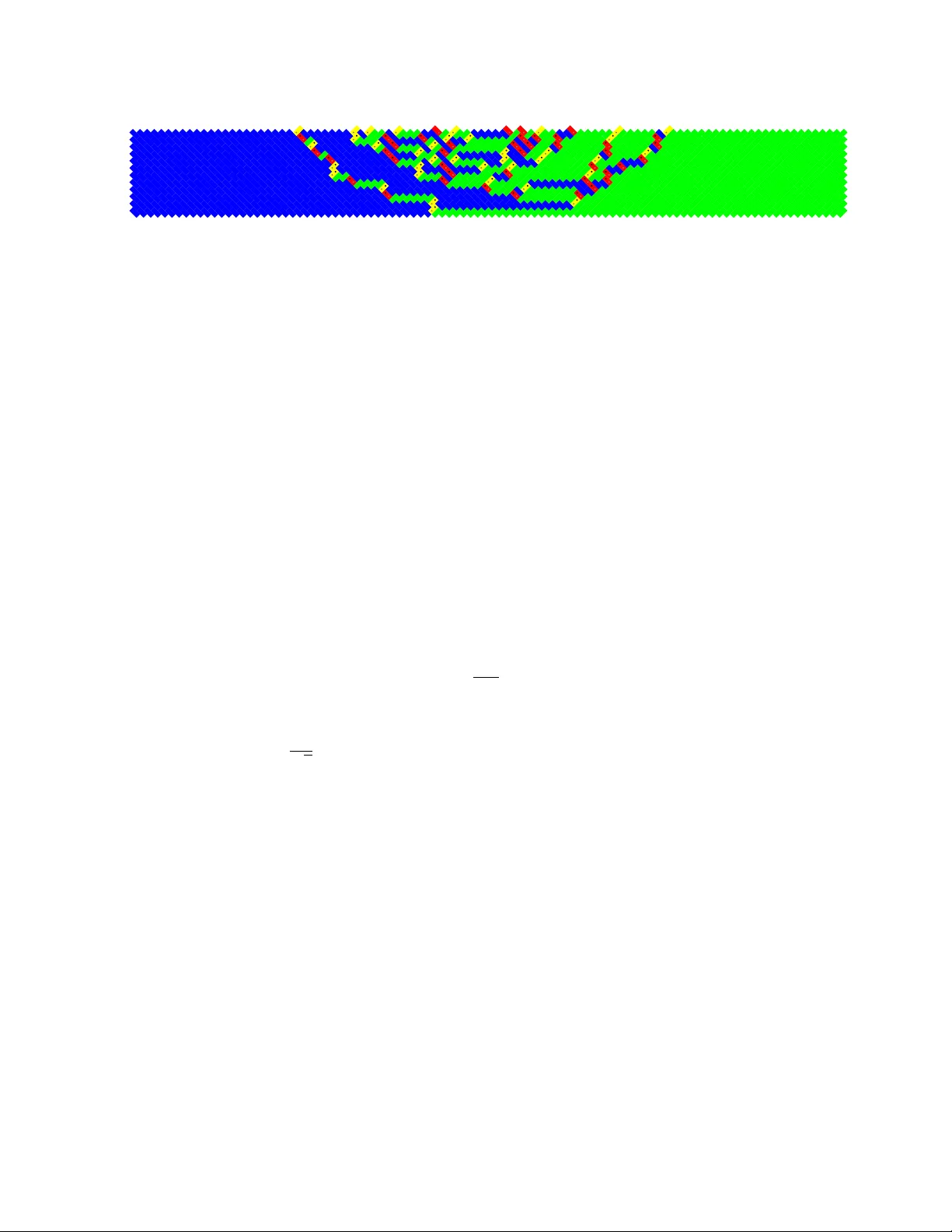
Mark ed GUE-corners pro cess in doubly p erio dic dimer mo dels T omas Berggren ∗ Nedialk o Bradinoﬀ † Abstract W e study a family of p eriodically w eighted Aztec diamond dimer mo dels near their turning p oin ts. W e establish that, asymptotically , as N → ∞ , their ﬂuctuations there, scaled b y √ N , are describ ed by a marked GUE-corners pro cess. This limiting p oint pro cess is constructed b y assigning a Bernoulli mark indep enden tly to each particle in a realization of the GUE-corners pro cess. The Bernoulli parameters asso ciated with the random marks reﬂect the p erio dicit y of the mo del in the limit. T o prov e this result w e use a double-contour integral represen tation of the inv erse Kasteleyn matrix on a higher-genus Riemann surface, which is well-suited for asymptotic analysis. Con ten ts 1 In tro duction 2 1.1 Preface . . . . . . . . . . . . . . . . . . . . . . . . . . . . . . . . . . . . . . . . . . . . 2 1.2 The Aztec diamond and an in terlacing particle system . . . . . . . . . . . . . . . . . 3 1.3 The GUE-corners process . . . . . . . . . . . . . . . . . . . . . . . . . . . . . . . . . 4 1.4 The marked GUE-corners pro cess . . . . . . . . . . . . . . . . . . . . . . . . . . . . . 4 1.5 Main results . . . . . . . . . . . . . . . . . . . . . . . . . . . . . . . . . . . . . . . . . 5 1.6 Outlo ok on further dev elopmen ts . . . . . . . . . . . . . . . . . . . . . . . . . . . . . 7 2 Preliminaries 8 2.1 The Aztec diamond dimer mo del . . . . . . . . . . . . . . . . . . . . . . . . . . . . . 8 2.2 An interlacing particle system . . . . . . . . . . . . . . . . . . . . . . . . . . . . . . . 9 2.3 The correlation k ernel and the sp ectral curve . . . . . . . . . . . . . . . . . . . . . . 11 3 Con vergence to the marked GUE-corners pro cess 14 4 Asymptotic analysis of the correlation Kernel 19 4.1 Establishing key prop erties of G ( z , w ) . . . . . . . . . . . . . . . . . . . . . . . . . . 21 4.2 Lo cal analysis at q ∞ and some global estimates . . . . . . . . . . . . . . . . . . . . . 24 4.3 Asymptotic analysis of J d . . . . . . . . . . . . . . . . . . . . . . . . . . . . . . . . . 29 4.4 Asymptotic analysis of J s . . . . . . . . . . . . . . . . . . . . . . . . . . . . . . . . . 35 4.5 Pro of of Theorem 3.3 . . . . . . . . . . . . . . . . . . . . . . . . . . . . . . . . . . . . 37 5 The parameters τ and σ 2 38 ∗ Departmen t of Mathematics & statistics, Univ ersity of South Florida, USA. E-mail: tb erggren@usf.edu † Departmen t of Mathematics, Ro yal Institute of T echnology , Sweden. E-mail: nedialko@kth.se 1 1 In tro duction 1.1 Preface Planar dimer mo dels take a central p osition in statistical mec hanics and com binatorics, serving as a rare class of t wo-dimensional lattice models that remain amenable to exact analysis. Beginning with the seminal works of Kasteleyn [36] and T emp erley–Fisher [46], which express the p artition function of a dimer model (equiv alen tly , the en umeration of dimer c overs or p erfe ct matchings ) in terms of determinan ts and Pfaﬃans, the sub ject has developed in to a vibrant area of research, with sustained activit y in the mathematical comm unity ov er the last three decades. Among the most accessible and inﬂuential instances are domino tilings of the Azte c diamond , introduced in [25, 26], where the “arctic circle phenomenon”–the co existence of frozen and disordered regions separated b y a sharp in terface known as the ar ctic curve –w as prov ed for the ﬁrst time [32]. This mo del subsequently b ecame a testing ground for general ideas in statistical mec hanics and particularly dimer models. The uniformly weigh ted Aztec diamond is by no w a classical mo del, and its lo cal and global statistics are well understo o d [14, 17, 21, 33]. Over the last decade, new analytic and algebraic to ols–com bining spectral curves, algebraic geometry , and reﬁned asymptotics–ha ve led to substantial progress for doubly p erio dic edge weigh ts. In this richer setting, the phase diagram ma y include not only fr ozen and r ough ( liquid ) regions, but also smo oth ( gase ous ) phases, reﬂecting the fact that the underlying sp ectral curv e t ypically has higher gen us [38]. F ollowing the initial analysis of the two-p erio dic Azte c diamond –the simplest instance in whic h a smo oth phase app ears–[16, 18, 24], the theory has developed rapidly: for general p eriodic w eights one now has explicit descriptions of limit shap es and arctic curv es [2, 4, 9], and detailed results on lo cal [4, 13] and global [7] ﬂuctuations, rev ealing new qualitativ e phenomena absen t in the uniform case. A natural question is then whether p eriodicity inﬂuences critical b eha vior, more precisely , the lo cal edge ﬂuctuations near the arctic curve. W e study this question near the turning p oints –the p oin ts where the arctic curve touches the b oundary . In the uniformly weigh ted Aztec diamond these lo cal ﬂuctuations are go verned by the GUE- c orners pro cess [35]. The GUE-corners pro cess is a multi-lev el determinantal p oin t pro cess deﬁned b y the eigen v alues of the principal leading sub-matrices of an inﬁnite GUE-matrix and has b y no w b een prov ed to b e a universal limit at turning p oin ts in uniformly w eighted lozenge tilings [1, 31, 41, 43]. In addition, the GUE-corners process has b een pro ved to go vern the limit around turning p oin ts also in plane partitions containing more than one turning p oin t on one side of the domain [40], as well as in the six-vertex mo del, [22, 23, 29]. V ery recen tly , the GUE-corners pro cess w as also observed in the t wo-perio dic Aztec diamond [45], see the last paragraph in Section 1.5 for more details. In this pap er, we study the corresp onding limit for a class of doubly p erio dic Aztec diamond dimer mo dels and sho w that the microscopic p erio dic structure surviv es in a nontrivial w ay: the limiting ob ject is a marke d GUE-c orners pr o c ess . Informally , the p eriodicity introduces intrinsic marks (or colors) that persist under the critical scaling, and the resulting correlation functions con verge to those of a mark ed extension of the classical GUE-corners ensem ble. Moreo ver, w e deﬁne, on the discrete level, a p oin t pro cess that conv erges to this limit. This iden tiﬁes a new mec hanism b y which p eriodic microscopic data enrich critical limits. 2 1 2 3 4 5 6 7 8 1 2 3 4 5 6 7 8 0 α 1 1 1 β 1 α 2 1 1 β 2 α 3 1 1 β 3 α 4 1 1 β 4 α − 1 1 1 1 β − 1 1 α − 1 2 1 1 β − 1 2 α − 1 3 1 1 β − 1 3 α − 1 4 1 1 β − 1 4 Figure 1: The Aztec diamond graph of size 4 on the left and the fundamen tal domain of the 2 × 4 p eriodically weigh ted Aztec diamond dimer mo del on the righ t. North, East, South, and W est edges are colored blue, orange, red, and green respectively . 1.2 The Aztec diamond and an in terlacing particle system The results in this w ork are in the context of the Azte c diamond dimer mo del (or the Azte c diamond ), a dimer mo del deﬁned on the Aztec diamond graph G Az . The Azte c diamond gr aph of size N is a bipartite graph deﬁned on a subset of { 0 , 1 , 2 , . . . , 2 N } 2 ⊂ Z 2 so that there are black v ertices on p oin ts with even x -co ordinate and o dd y -coordinate and white vertices at p oin ts with o dd x - co ordinate and even y -coordinate. T wo v ertices are adjacent if b oth their co ordinates diﬀer b y exactly 1 , see Figure 1. Dep ending on the vertices they are adjacent to, the edges (and their corresp onding dimers in a random outcome) are classiﬁed as North, South, East, or W est. A p erfe ct matching or dimer c over of G Az is a subgraph of G Az in which eac h v ertex is incident to exactly one edge ( dimer ). One in tro duces a weigh t to each edge and the asso ciated dimer mo del on the graph is pro duced b y selecting a random p erfect matching on the graph with probabilit y proportional to the product of the weigh ts of the edges in that matching. In this w ork the weigh ts put on the edges are selected p eriodically with p erio d ℓ in the x co ordinate and p eriod 2 in the y co ordinate. W e introduce 2 ℓ parameters, α 1 , . . . , α ℓ , β 1 , . . . , β ℓ > 0 and distribute them on the fundamental domain of size 2 × ℓ as in Figure 1, see (2.1) b elow for a precise deﬁnition. W e imp ose the additional constraint that Q ℓ i =1 α i = Q ℓ i =1 β i and th us are in the setting studied in [3]. F or clarity we restrict our attention to the Aztec diamond of size 2 ℓN . One wa y to describ e a given dimer co ver is to describ e whic h v ertices are inciden t to a South or W est dimer, and, following [33], w e place black/white particles at suc h black/white vertices. If w e restrict our attention to either only the white particles or only the blac k particles we get an in terlacing particle system. Here w e consider particles with the same x co ordinate to lie on the same lev el and we enumerate the levels from the righ t ( x = 2 ℓN ) to the left ( x = 0) . This interlacing particle system is set to capture the lo cal ﬂuctuations around the turning p oin t with co ordinate x = 2 ℓN . The t wo in terlacing particle systems corresp onding to the white and black v ertices are 3 Figure 2: The tw o in terlacing particle systems near the turning p oin t, in grey and blac k, deﬁned from South (y ellow) and W est (red) edges from a random outcome of the Aztec diamond; The picture is rotated so that the ﬁrst particle is at the b ottom instead of to the right. Dimers in the picture are illustrated as domino es. closely related, see Figure 2. Pro ceeding with the conv en tion in [33] we restrict our atten tion to blac k v ertices adjacen t to a South or W est edge and study the p oin t pro cess describ ed by them, ( u t s ) 1 ≤ s ≤ t . It turns out signiﬁcant for the studied pro cess in this work that the t wo p eriodicity of the weigh ts along the y axis giv es rise to a natural further coloring of these particles; we color them red if their y co ordinate is ev en and cyan if it is odd, see prescribed colors in Figure 3. En umerated from the righ t to the left the colored particles describ e a (colored) in terlacing particle system, ( u t s,j ) 1 ≤ s ≤ t , where j ∈ { 0 , 1 } indicates the color asso ciated to eac h particle, t is its level, and s is its relativ e p osition with resp ect to the particles on the same lev el. 1.3 The GUE-corners pro cess The GUE-c orners pr o c ess (also kno wn as the GUE minor pr o c ess ), P GUE , is a determinantal p oint pr o c ess on Λ = Z > 0 × R . One wa y in which it can b e constructed is b y taking a random Z > 0 × Z > 0 hermitian matrix, X = ( X ij ) i,j ∈ Z > 0 with X ij = X j i suc h that the entries ab o ve and on the main diagonal ( i = j ) are indep enden t random v ariables with X ij ∼ 1 √ 2 ( N (0 , 1) + iN (0 , 1)) for i > j, and X ii ∼ N (0 , 1) . Then for t ∈ Z > 0 the top left t × t corner of X , X ( t ) = ( X ij ) 1 ≤ i,j ≤ t is distributed as a GUE( t ) matrix with ordered eigen v alues ξ t 1 ≤ ξ t 2 ≤ . . . ≤ ξ t t , and the matrix X couples the eigenv alues on diﬀerent lev els so that they interlace, namely ξ t +1 s ≤ ξ t s ≤ ξ t +1 s +1 and the pro cess giv en b y  ξ t s  1 ≤ s ≤ t,t ∈ Z > 0 deﬁnes the GUE-corners pro cess. That this pro cess is well-deﬁned is explained, for instance, in [35]. 1.4 The marked GUE-corners pro cess A deﬁning feature in this w ork is the emergence of a marke d p oint pr o c ess in the limit of the in terlacing particle system as N → ∞ ; the limiting p oin t pro cess “remem b ers” the colors of the p oin ts coming from the 2 perio dicity in the v ertical direction. F or a measurable function θ : Λ → [0 , 1] we call the marke d GUE-c orners pro cess, P θ GUE , the p oint pro cess on Λ { 0 , 1 } = Λ × { 0 , 1 } constructed out of the GUE-corners pro cess on Λ b y indep enden tly assigning to each p oin t a binary v alue; a mark m ∼ Bernoulli( θ ( t, µ )) , where ( t, µ ) ∈ Λ is the lo cation of the p oin t. W e denote these marked particles by ( ξ t s,j ) 1 ≤ s ≤ t , where j ∈ { 0 , 1 } 4 represen ts the marking. It was pro ved in [19] – for a general determinan tal p oin t pro cess under very mild assumptions – that the point process P θ GUE is a determinan tal p oin t pro cess with correlation k ernel K θ GUE ( t 1 , µ 1 , j 1 ; t 2 , µ 2 , j 2 ) = ( θ ( t 1 , µ 1 ) δ 1 j 1 + (1 − θ ( t 1 , µ 1 )) δ 0 j 1 ) K GUE ( t 1 , µ 1 ; t 2 , µ 2 ) , (1.1) where δ j j ′ is the Kronec k er delta function. Mark ed point pro cesses w ere in tro duced and studied in [19], with the interpretation that a particle is observ ed or not in a measuremen t dep ending on the v alue of the mark. The purpose of that pap er w as to study certain conditional probabilities of these marked processes. This was later used to study certain deformations of biorthogonal ensem bles [20]. 1.5 Main results F or the c hoice of w eights considered in this pap er, there are four turning p oints –p oin ts where the ar ctic curve touches the b oundary of the Aztec diamond–one on each side of the Aztec diamond. W e fo cus in this work on the right-most turning p oin t with co ordinates (2 ℓN , 2 τ N ) for some τ > 0 (whic h we determine). The ﬂuctuations around this turning p oin t are captured by the particle system ( u t s ) 1 ≤ s ≤ t ≤ 2 ℓN . The unique particle on the ﬁrst level is distributed around the right-most turning p oin t with ﬂuctuations of order √ N , similarly to the uniform case. Thus we center the v ertical coordinates of the studied pro cess at 2 τ N and rescale by √ N , while we do not rescale the horizon tal co ordinate. The new co ordinates are ( t, µ ) ∈ Λ = Z > 0 × R . The process constructed in this fashion in the case of the Aztec diamond with uniform weigh ts is classically kno wn to con verge to the celebrated GUE-corners pro cess [35]. In this work we pro ve that the corresp onding limit in the 2 × ℓ perio dic setting is aﬀected by the 2-p erio dicit y in the vertical direction. The particle system ( u t s ) 1 ≤ s ≤ t ≤ 2 ℓN is a determinantal p oin t pro cess with correlation kernel K Int , see Theorem 2.4 b elo w. W e study its ﬂuctuations around the turning p oint via this correlation k ernel. The coordinates of the correlation k ernel are naturally expressed b y ( ℓx + i, 2 y + j ) for i = 0 , . . . , ℓ − 1 and j = 0 , 1 , and in those co ordinates, the co ordinate of the black v ertex asso ciated with u t s is ( ℓx + i, 2 y + j ) = (2 ℓN − t, u t s ) . The centering at the turning p oin t and scaling discussed ab o v e, is then given by y = ⌊ N τ + √ N µ ⌋ . W e ha ve the following result for the limiting correlation k ernel of the pro cess under the describ ed scaling. Theorem 1.1 (Theorem 3.3) . L et K Int b e the c orr elation kernel of ( u t s ) 1 ≤ s ≤ t ≤ 2 ℓN and supp ose ν : Z > 0 × { 0 , 1 } → R is given by ν ( t, j ) =      1 1+ α ℓ +1 − t β − 1 ℓ − t if j = 0 , α ℓ +1 − t β − 1 ℓ − t 1+ α ℓ +1 − t β − 1 ℓ − t if j = 1 , wher e α ℓ − t and β ℓ − t ar e the e dge weights of the mo del (se e Figur e 1 and later (2.1) ). L et the gauge function g : { 0 , 1 , . . . , 2 ℓN } 2 → R b e deﬁne d by (3.4) and let τ , σ > 0 b e (explicitly) given by (3.1) and (3.5) b elow. Set ℓx k + i k = 2 ℓN − t k and y k = ⌊ N τ + √ N µ k ⌋ , for k = 1 , 2 . Then, for µ 1  = µ 2 , lim N →∞ g ( ℓx 1 + i 1 , 2 y 1 + j 1 ) g ( ℓx 2 + i 2 , 2 y 2 + j 2 ) N 1 2 K Int ( ℓx 1 + i 1 , 2 y 1 + j 1 ; ℓx 2 + i 2 , 2 y 2 + j 2 ) = ν ( t 2 , j 2 ) σ − 1 K GUE ( t 1 , σ − 1 µ 1 ; t 2 , σ − 1 µ 2 ) , 5 wher e K GUE ( t 1 , µ 1 ; t 2 , µ 2 ) = 1 (2 π i) 2 ˆ γ ′ s ˆ γ ′ l e 1 2 ( z 2 2 − z 2 1 ) e µ 1 z 1 − µ 2 z 2 z t 2 2 z t 1 1 d z 1 d z 2 z 2 − z 1 , is the c orr elation kernel of the GUE-c orners pr o c ess. The se quenc e on the left-hand side is uniformly b ounde d in N on c omp act subsets of Λ 2 { 0 , 1 } with r esp e ct to the emb e dding given by ( t p , µ p , j p ) ∈ Λ { 0 , 1 } , for p = 1 , 2 . Se e The or em 3.3 for a deﬁnition of the curves γ ′ s and γ ′ ℓ . The correlation k ernel K GUE as presented here was obtained in [35, 43]. The factor ν ( t 2 , j 2 ) in the limit c hanges the limiting k ernel non-trivially and cannot b e remov ed via a gauge. In fact the limiting function is the correlation k ernel of a mark ed GUE-corners pro cess instead of the GUE-corners pro cess. Indeed, if θ ( t, µ ) = θ ( t ) = α ℓ +1 − t β − 1 ℓ − t 1 + α ℓ +1 − t β − 1 ℓ − t , (1.2) then ν ( t, j ) = θ ( t ) δ 1 j + (1 − θ ( t )) δ 0 j is the pre-factor in (1.1). By studying the colored interlacing system ( u t s,j ) 1 ≤ s ≤ t , we can in terpret the conv ergence of the correlation functions in Theorem 1.1 as a con v ergence of pro cesses. Theorem 1.2 (Corollary 3.7) . L et ( u t s,j ) 1 ≤ s ≤ t ≤ 2 ℓN b e the c olor e d interlacing p article system de- scrib e d ab ove. Then ther e ar e (explicit) τ , σ > 0 (se e later (3.1) and (3.5) ) such that the turning p oint has c o or dinates (2 ℓN , 2 τ N ) and u t s,j − 2 N τ 2 σ √ N ! 1 ≤ s ≤ t →  ξ t s,j  1 ≤ s ≤ t , in the sense of we ak c onver genc e as N → ∞ , and ( ξ t s,j ) 1 ≤ s ≤ t is the marke d GUE-c orners pr o c ess with an underlying marking function θ given in (1.2) . The ab o ve theorems sho w that the discreteness of the fundamental domain p ersists in the scaling limit, although the horizon tal and vertical p erio dicities are enco ded in diﬀerent wa ys. The horizon tal ℓ -p eriodicity is retained through the parameter θ , which dep ends on t –more precisely , on the edge w eights in the “ ℓ + 1 − t column” of the fundamental domain. By con trast, the v ertical 2 -p erio dicit y is carried by the marks j ∈ { 0 , 1 } . W e conjecture that if the mo del instead is k -p eriodic in the v ertical direction, then the limit will b e a k -marke d GUE-corners pro cess; to each outcome of the p oin t pro cess one assigns indep enden tly a random integer b et w een 0 and k − 1 . It is in teresting–and somewhat surprising–that, even though the y -co ordinate is rescaled and con verges to a con tin uous coordinate µ , a trace of the microscopic structure surviv es via these marks. Moreo ver, once the discreteness p ersists in this form, it is not obvious a priori that the con tributions asso ciated with the tw o marks should decouple, i.e., that the marks should b eha ve indep enden tly . Mark ed pro cesses are closely related to thinne d pr o c esses . A thinned process is deﬁned b y indep enden tly deleting each particle of a giv en pro cess with some probability . These pro cesses were in tro duced in the random matrix theory literature b y [10, 11] with the motiv ation b ehind their study b eing to mo del situations in whic h the p ossibilit y of failed detection/measuremen t of particles may 6 o ccur. They hav e since b een studied in many contexts within the random matrix theory literature, for instance, in [5, 12, 15]. In the dimer literature a thinned pro cess was observed in [17], as the authors studied the pro cess deﬁned b y viewing only the south dimers as particles in the biase d Azte c diamond . Theorem 1.2 implies that if we study the pro cess describ ed b y only the red or only the cyan particles w e get a thinne d GUE-corners pro cess as a limiting pro cess; that is, a GUE-corners pro cess in which each particle is deleted independently with probability 1 − θ or θ , respectively . Corollary 1.3 (Corollary 3.9) . The r estriction of the p oint pr o c ess ( u t s,j ) 1 ≤ s ≤ t ≤ 2 ℓN to p oints with j = 1 c onver ges, under the same sc aling and in the same sense as in The or em 1.2, to a thinne d GUE–c orners pr o c ess with deletion pr ob ability θ . W e stress that the limit in Theorem 1.2 is subtle. If one identiﬁes the t wo colors (equiv alently , forgets the marks), one recov ers the classical GUE-corners pro cess (see Remark 3.8 b elo w). In our framew ork, ho w ever, the marks arise naturally , as seen from Theorem 1.1. While this manuscript was b eing prepared, the pap er [45] app eared. In that w ork, the authors analyse the same limiting regime in the sp ecial case of the t wo-perio dic Aztec diamond (in our notation ℓ = 2 , and α − 1 1 = β − 1 1 = α 2 = β 2 = a for some a > 0 ) using a completely diﬀeren t metho d. Ho wev er, it app ears that their metho d do es not capture this reﬁned limit; instead, the classical (unmark ed) GUE-corners pro cess is obtained. 1.6 Outlo ok on further dev elopmen ts Let us brieﬂy sp ecialize to the tw o-p erio dic Aztec diamond. This mo del dep ends on a single pa- rameter a ; in our notation ℓ = 2 and α − 1 1 = β − 1 1 = α 2 = β 2 = a . In this case the marking function θ simpliﬁes to θ ( t, µ ) = ( a 2 1+ a 2 , t o dd, a − 2 1+ a − 2 , t even. Th us, as a → 0 or a → ∞ , we ha ve θ ( t, µ ) → 0 or 1 (dep ending on the parity of t ), so the marks b ecome asymptotically deterministic. In particular, after forgetting the now-trivial marks, one recov ers the classical GUE-corners process in this limit. A t the same time, the global geometry c hanges as a → 0 or a → ∞ : the rough region shrinks a wa y , while the smo oth phase turns into a tilted square that meets the frozen regions. In particular, the smo oth phase reac hes the turning p oin t, and the lo cal conﬁguration there app ears to freeze. These observ ations suggest a natural tw o-parameter asymptotic question: let the weigh ts v ary with the size N and consider a scaling limit in which a = a ( N ) → ∞ . If a ( N ) div erges suﬃcien tly slo wly compared with N , one should see the GUE-corners pro cess. At the opp osite extreme, if a ( N ) diverges very rapidly , the particles should freeze and the conﬁguration becomes essentially deterministic. Understanding the intermediate regime b et w een these extremes would be particularly interesting. It is tempting to sp eculate that an appropriate interpolation limit might b e related to the ∞ -corners pro cess studied in [28, 30]. While an in termediate scaling regime has b een analyzed along the frozen- smo oth in terface in [34], the corresponding behavior at the turning p oin t appears to remain op en. One can attempt to extend the abov e discussion to more general p erio dic weigh ts. In [9], a temp erature parameter is introduced and the corresponding zero-temp erature limit is analyzed. In that limit, the limit shap e conv erges to a piecewise linear proﬁle, and–muc h as in the tw o-p eriodic 7 Aztec diamond–the rough region v anishes and the smo oth phase expands so as to reac h the turning p oin ts. This raises a natural question: in such a joint scaling regime (with N → ∞ and temp erature tending to zero), to what extent is the turning-p oin t b eha vior universal, and to what extent do es it dep end on the speciﬁc c hoice of w eights? Outline of the pap er. The necessary bac kground for this w ork, including a double-con tour in tegral expression for the inv erse Kasteleyn matrix obtained in [3] (see Theorem 2.4), is in tro duced in Section 2. W e state and prov e our main results in Section 3, deferring the technical analysis of the double-con tour in tegral to Section 4. The explicit computation of the parameters τ and σ app earing in Theorem 1.2 is then giv en in Section 5. A ckno wledgements W e are grateful to Maurice Duits for all the v aluable discussions throughout this pro ject. Nedialk o Bradinoﬀ was supp orted by the Europ ean Research Council (ERC), Grant Agreemen t No. 101002013. 2 Preliminaries W e discuss in more detail the necessary bac kground and con text of this work. 2.1 The Aztec diamond dimer mo del In this section we deﬁne the Aztec diamond dimer mo del. The Aztec diamond graph G Az = ( B Az , W Az , E Az ) of size N is a bibartite graph deﬁned from a subset of the tilted square lattice. More precisely , set B Az = { (2 i, 2 j + 1) : i ∈ { 0 , . . . , N } , j ∈ { 0 , . . . , N − 1 }} , and W Az = { (2 i + 1 , 2 j ) : i ∈ { 0 , . . . , N − 1 } , j ∈ { 0 , . . . , N }} . The set of vertices of G Az is the union B Az ∪ W Az , where we call B Az black vertic es and W Az white v ertices. The edges E Az consists of the union of four type of edges, north , e ast , south , and west edges: north = { ((2 i − 1 , 2 j ) , (2 i, 2 j − 1)) : (2 i − 1 , 2 j ) ∈ W Az , (2 i, 2 j − 1)) ∈ B Az } , east = { ((2 i − 1 , 2 j ) , (2 i, 2 j + 1)) : (2 i − 1 , 2 j ) ∈ W Az , (2 i, 2 j + 1)) ∈ B Az } , south = { ((2 i + 1 , 2 j ) , (2 i, 2 j + 1)) : (2 i + 1 , 2 j ) ∈ W Az , (2 i, 2 j + 1)) ∈ B Az } , w est = { ((2 i + 1 , 2 j ) , (2 i, 2 j − 1)) : (2 i + 1 , 2 j ) ∈ W Az , (2 i, 2 j − 1)) ∈ B Az } . T o in tro duce the dimer model, we introduce edge weigh ts α i , β i > 0 for i ∈ Z , and deﬁne the w eight function w : E Az → R > 0 as follo ws: Let e south = ((2 i + 1 , 2 j ) , (2 i, 2 j + 1)) ∈ E Az and e east = ((2 i − 1 , 2 j ) , (2 i, 2 j + 1)) ∈ E Az b e a south and east edge. F or e ∈ E Az , we set w ( e ) =                α − 1 i +1 , e = e south , j even , α i +1 , e = e south , j o dd , β − 1 i , e = e east , j even , β i , e = e east , j o dd , 1 , otherwise . (2.1) 8 By deﬁnition, the w eight function w is 2 -p erio dic in the vertical direction, that is, 2 -p erio dic in the j co ordinate. W e will also assume it is perio dic in the horizon tal direction, that is, p eriodic in the i coordinate, let sa y with perio d ℓ . W e therefore assume that α i + ℓ = α i and β i + ℓ = β i for all i . In addition, following [3], w e will assume that Q ℓ i =1 α i = Q ℓ i =1 β i . F or simplicity , w e also imp ose the generic assumption that the asso ciated sp ectral curv e has maximum gen us, that is, g = ℓ − 1 , see Section 2.3. Giv en the graph G Az and the w eight function w , we deﬁne a probabilit y measure on all dimer c overs of the Aztec diamond. Recall that a dimer co v er D of G Az is a subset of E Az suc h that eac h v ertex in B az and W Az is adjacent to exactly one edge in D . An element in D is called a dimer . W e consider here the Boltzmann measure, P dimer ( D ) = 1 Z Y d ∈D w ( d ) , (2.2) where Z = P D Q d ∈D w ( d ) is called the p artition function and the sum is o ver all p ossible dimer co vers D of G Az . The edge inclusion probabilit y , that is, the probability to see a sp eciﬁc set of dimers in a dimer co ver can b e expressed in terms of the Kasteleyn matrix K Az and its inv erse. T o deﬁne the Kasteleyn matrix, we introduce the Kasteleyn sign σ : E Az → {− 1 , 1 } by letting σ ( e ) = − 1 if e is a north edge and σ ( e ) = 1 otherwise. In general, the Kasteleyn sign can b e c hosen to tak e v alues on the unit circle with the condition that the alternating pro duct around each face of the graph is ( − 1) k +1 , where 2 k is the num b er of edges around the face. The Kasteleyn matrix K Az is essentially a weigh ted adjacency matrix: K Az : C B Az → C W Az , deﬁned as K Az (w , b) = 1 wb ∈E Az σ (wb) w (wb) , (2.3) where w ∈ W Az and b ∈ B Az . The expression on the righ t-hand side should be interpreted as zero if wb is not an edge. The Kasteleyn signs are deﬁned so that Z = | det K Az | [36, 46], and it follo ws [37] that for k edges b p w p ∈ E Az , p = 1 , . . . , k , P dimer (b p w p ∈ D for all p = 1 , . . . , k ) = det  K Az (w p ′ , b p ′ ) K − 1 Az (b p , w p ′ )  k p,p ′ =1 . (2.4) In general it is a hard problem to obtain a suitable expression for the inv erse Kasteleyn matrix. In the setting considered here, the inv erse Kasteleyn matrix, or rather, the correlation k ernel for the asso ciated non-in tersecting path mo del, was obtained in [3] using the tec hnique developed in [6]. 2.2 An interlacing particle system The dimer mo del discussed in the previous section is a determinantal p oint pr o c ess , where the dimers are view ed as points and the c orr elation kernel can b e expressed in terms of the Kasteleyn matrix and its in verse. In this paper, we are in terested in a closely related p oin t pro cess. Namely , giv en a dimer cov er D of G Az , w e deﬁne a p oin t conﬁguration by putting a point, or particle, at a black v ertex b ∈ B Az if b is adjacent to a south or w est edge in D . See Figure 3. The probabilit y measure P dimer in (2.2) induces a probability measure P Int on the set of p oin t conﬁgurations deﬁned ab o v e. W e sa y that a blac k v ertex is on the 2 i th level if its ﬁrst coordinate is 2 i . Similarly , w e say that a white v ertex with ﬁrst co ordinate 2 i + 1 is on level 2 i + 1 . 9 j ev en j o dd east north w est south Figure 3: Left: The particles deﬁned from the dimers visualized in red and cyan. The color dep ends on the parity of the coordinates of the particle. Right: A dimer co ver of the Aztec diamond of size 4 . The particles form an in terlacing particle system. Lemma 2.1. Fix a dimer c over D of G Az and i ∈ { 0 , . . . , N } . The black vertic es on level 2 i ar e adjac ent to N − i south or west dimers. Pr o of. On each even lev el, there are N black v ertices and on each o dd lev el, there are N + 1 white v ertices. If there are k black vertices on level 2 i that are adjacen t to a south or west dimer, it means that there hav e to be N + 1 − k black v ertices on lev el 2( i + 1) adjacen t to a north or east dimer, since all white vertices on level 2 i + 1 ha ve to b e adjacent to some dimer. Consequently , there are k − 1 black vertices adjacent to a south or west dimer on lev el 2( i + 1) . Since there are N v ertices on lev el 0 that are adjacen t to a south or w est dimer, w e ha v e pro v ed the statement. The previous lemma shows that the p oin t pro cess in tro duced in the b eginning of this section can naturally b e denoted b y { u t s } 1 ≤ s ≤ t ≤ N where u t s ≤ u t s +1 and lies on level N − t . In particular, the co ordinate of the black v ertex associated with u t s is (2( N − t ) , 2 u t s + 1) . Lemma 2.2 ([35]) . The p oint pr o c ess { u t s } 1 ≤ s ≤ t ≤ N is an interlacing p article system, that is, u t +1 s ≤ u t s ≤ u t +1 s +1 . Pr o of. Pic k a blac k v ertex b = (2 i, 2 j + 1) and let b ′ = (2( i + 1) , 2 j + 1) b e the blac k vertex immediately to its right. Supp ose there are k particles whose v ertical co ordinate is less than or equal to that of b . By an argument analogous to that in the pro of of Lemma 2.1, there are either k or k − 1 particles whose v ertical co ordinate is less than or equal to that of b ′ . Since this holds for all black vertices, it follo ws that if there are k particles at or b elo w b ′ , then there must b e a particle lo cated at b ′ . Let b corresp ond to the blac k vertex asso ciated with u t +1 s , and b ′ to the black vertex immediately to its right. If there are k particles at or below b and also k particles at or below b ′ , then a particle occupies b ′ , implying u t +1 s = u t s < u t +1 s +1 . If instead there are k − 1 particles at or below b ′ , then u t +1 s < u t s , and moreo ver, we must hav e u t s ≤ u t +1 s +1 to preserve the prop ert y established at the b eginning of the proof. T o capture the p eriodicity in the underlying dimer mo del, w e color the particles of the p oin t pro cess { u t s } 1 ≤ s ≤ t in tw o diﬀerent colors dep ending on the lo cation, see Deﬁnition 3.6 b elow. 10 2.3 The correlation kernel and the sp ectral curv e In the uniform case, α i = β i = 1 , for all i , it was prov ed in [33] that the p oin t pro cess { u t s } 1 ≤ s ≤ t is a determinan tal point pro cess with correlation k ernel determined from non-in tersecting paths known as the DR-paths. More precisely , the p oin t pro cess is the restriction of the p oin t pro cess deﬁned from the non-intersecting paths to the even levels. In our setting, the same argument holds and the correlation kernel for the p oin t pro cess { u t s } 1 ≤ s ≤ t is the restriction of the correlation kernel given in [3] restricted to the ev en lev els. T o express the correlation k ernel we deﬁne the follo wing 2 × 2 matrices: ϕ 2 i − 1 ( z ) =  1 α − 1 i z − 1 α i 1  , and ϕ 2 i ( z ) = 1 1 − z − 1  1 β − 1 i z − 1 β i 1  , (2.5) for i = 1 , . . . , ℓ . W e denote the pro duct of these matrices by Φ = Q 2 ℓ m =1 ϕ m . Note that det Φ( z ) = 1 . The correlation k ernel is naturally describ ed as a double con tour integral on a higher genus Riemann surface. W e discuss this Riemann surface b efore w e recall the in tegral formulation of the correlation kernel. The characteristic p olynomial P of the dimer mo del is giv en by P ( z , w ) = (1 − z − 1 ) ℓ det(Φ( z ) − w I ) , and the spectral curv e is deﬁned by R ◦ = { ( z , w ) ∈ ( C ∗ ) 2 : P ( z , w ) = 0 } , where C ∗ = C \{ 0 } . It was prov ed in [3] that the c haracteristic polynomial deﬁned here coincides with the c haracteristic p olynomial deﬁned in [38]. The sp ectral curve introduced in [38] w as prov ed to be a so-called Harnack curve – a sp eciﬁcally nice t yp e of curve. Since the tw o sp ectral curves coincide, R ◦ is a Harnack curve. The sp ectral curve is naturally compactiﬁed in an appropriate toric surface, and we denote this compactiﬁcation by R . Concretely , R = R ◦ ∪ { p 0 , p ∞ , q 0 , q ∞ } , where p 0 = (0 , 1) , p ∞ = ( ∞ , 1) , q 0 = (1 , 0) , q ∞ = (1 , ∞ ) . This Riemann surface was describ ed in [3] by gluing together tw o copies of C along interv als of the negativ e part of the real line. W e describe that construction b elo w. Lemma 2.3 ([3]) . L et Disc w ( P ) b e the discriminant of the p olynomial P in the variable w , and let p ( z ) = z 2 ℓ Disc w ( P ) . Then p ( z ) =  ( z − 1) ℓ T r Φ( z )  2 − 4( z − 1) 2 ℓ . The function p is a de gr e e 2 ℓ − 1 p olynomial with zer os 0 = z 0 > z 1 ≥ z 2 > z 3 ≥ z 4 > · · · > z 2 ℓ − 3 ≥ z 2 ℓ − 2 . T o see that p is the discriminan t of P , w e use that det Φ( z ) = 1 . It follo ws from the deﬁnition of R , that the zeros of the p olynomial p from the previous lemma are the branc h p oints of the Riemann surface. The cuts along whic h we glue together the t wo copies of C are tak en b et w een z 2 k and z 2 k +1 for k = 0 , . . . , ℓ − 1 , where we set z 2 ℓ − 1 = −∞ . The real part of R consists of ℓ 11 p 0 p ∞ q ∞ ˜ Γ s ˜ Γ l p 0 p ∞ q 0 A 0 A 1 A 2 Figure 4: The Riemann surface R represente d as tw o copies of the complex plane. The cuts (dashed) are lo cated along the negative part of the real lines. The compact ov als A k , k = 1 , . . . , ℓ − 1 (solid) are lo cated along the negativ e part of the real lines, and the non-compact ov al A 0 (solid) are lo cated along the p ositiv e part of the real lines. The gra y areas are connected via the cuts, and so are the white areas. In this illustration, the curv e ˜ Γ s (blue) is a simple loop, while ˜ Γ l (red) is the union of t wo simple lo ops. connected comp onen ts A k , k = 0 , . . . , ℓ − 1 , that are kno wn as ovals . F or k = 1 , . . . , ℓ − 1 , w e set A k = { ( z , w ) ∈ R : z 2 k − 1 ≥ z ≥ z 2 k } and we refer to them as the c omp act ovals . F or k = 0 , the o v al is referred to as the non-c omp act oval and is given b y A 0 = { ( z , w ) ∈ R : 0 ≤ z ≤ + ∞} . By Lemma 2.3, the cuts cannot shrink to a p oint for an y choice of p ositiv e edge w eights, while the compact ov als can b e points. This means that the genus g of R , is b ounded ab o ve by ℓ − 1 . F or simplicit y , we assume throughout the paper, that g = ℓ − 1 . See Figure 4 for an illustration of the Riemann surface R . F or a simple closed curve ˜ Γ in R , we deﬁne the exterior of ˜ Γ as the connected comp onen t of R\ ˜ Γ that contains p ∞ = ( ∞ , 1) . The complement of the exterior is called the interior of ˜ Γ . The curv e ˜ Γ is p ositiv ely orien ted if the interior is to the left of the curve. W e are ready to express the correlation k ernel for the point pro cess { u t s } 1 ≤ s ≤ t ≤ N . T o simplify notation, we write Q ( z , w ) = adj( w I − Φ( z )) ∂ w det( w I − Φ( z )) . (2.6) F or simplicity , w e will assume that the size of the Aztec diamond is 2 ℓN instead of N . W e also write (2( ℓx + i ) , 2(2 y + j ) + 1) , where x = 0 . . . , 2 N − 1 , i = 0 , . . . , ℓ − 1 , y = 0 , . . . , ℓN − 1 , and j = 0 , 1 , instead of (2 i, 2 j + 1) , and identify these p oin ts with ( ℓx + i, 2 y + j ) . Recall also that the co ordinate of the black v ertex associated with u t s is ( ℓx + i, 2 y + j ) = (2 ℓN − t, u t s ) . Theorem 2.4. L et ρ Int k = ρ Int k,N b e the k th c orr elation function asso ciate d to the p oint pr o c ess { u t s } 1 ≤ s ≤ t ≤ 2 ℓN . F or k black p oints ( ℓx p + i p , 2 y p + j p ) , p = 1 , . . . , k , wher e x p = 0 . . . , 2 N − 1 , i p = 0 , . . . , ℓ − 1 , y p = 0 , . . . , ℓN − 1 , and j p = 0 , 1 , we have ρ Int k ( ℓx 1 + i 1 , 2 y 1 + j 1 ; . . . ; ℓx k + i k , 2 y k + j k ) = det  K Int  ℓx p + i p , 2 y p + j p ; ℓx p ′ + i p ′ , 2 y p ′ + j p ′  k p,p ′ =1 , 12 wher e  K Int ( ℓx + i, 2 y + j ; ℓx ′ + i ′ , 2 y ′ + j ′ )  1 j ′ ,j =0 = − 1 ℓx + i>ℓx ′ + i ′ 2 π i ˆ ˜ Γ l 2 i ′ Y m =1 ϕ m ( z ) ! − 1 Q ( z , w ) 2 i Y m =1 ϕ m ( z ) w x − x ′ z y ′ − y d z z + 1 (2 π i) 2 ˆ ˜ Γ s ˆ ˜ Γ l 2 i ′ Y m =1 ϕ m ( z 1 ) ! − 1 Q ( z 1 , w 1 ) Q ( z 2 , w 2 ) 2 i Y m =1 ϕ m ( z 2 ) × ( z 2 − 1) ℓN ( z 1 − 1) ℓN w x − N 2 w x ′ − N 1 z y ′ 1 z y 2 d z 2 d z 1 z 2 ( z 2 − z 1 ) . (2.7) The c ontours ˜ Γ l and ˜ Γ s ar e simple close d p ositively oriente d curves in R c ontaining p 0 and q ∞ in their interior, and p ∞ and q 0 in their exterior. Mor e over, ˜ Γ s is c ontaine d in the interior of ˜ Γ l . Pr o of. Since we consider a point pro cess on a discrete space, ρ Int k ( ℓx 1 + i 1 , 2 y 1 + j 1 ; . . . ; ℓx k + i k , 2 y k + j k ) = P Int ( particles at b 1 , . . . , b k ) , (2.8) where b p = (2( ℓx p + i p ) , 2(2 y p + j p ) + 1) for p = 1 , . . . , k . By deﬁnition of the interlacing particle system, the probability on the right-hand side of (2.8) can b e expressed in terms of P dimer : F or a blac k vertex b p = (2( ℓx p + i p ) , 2(2 y p + j p ) + 1) and q = 0 , 1 , let w pq = (2( ℓx p + i p ) + 1 , 2(2 y p + j p + q )) b e the adjacent white v ertex so that b p w pq is a south edge if q = 0 and a w est edge if q = 1 . Then P Int ( particles at b 1 , . . . , b k ) = P dimer (b p w p 0 ∈ D or b p w p 1 ∈ D for all p = 1 , . . . , k ) . (2.9) Since b p w p 0 ∈ D and b p w p 1 ∈ D are disjoin t even ts, the righ t-hand side of (2.9) is equal to X ( q 1 ,...,q k ) ∈{ 0 , 1 } k P dimer  b p w pq p ∈ D for all p = 1 , . . . , k  , (2.10) where the sum runs ov er all k -tuple in { 0 , 1 } k . The terms in (2.10) are of the form (2.4), and the sum is therefore a sum ov er determinants. By the multilinearit y of determinan ts, (2.10) is equal to X ( q 1 ,...,q k ) ∈{ 0 , 1 } k det  K Az (w p ′ q p ′ , b p ′ ) K − 1 Az (b p , w p ′ q p ′ )  k p,p ′ =1 = det   X q p ′ ∈{ 0 , 1 } K Az (w p ′ q p ′ , b p ′ ) K − 1 Az (b p , w p ′ q p ′ )   k p,p ′ =1 . (2.11) What is left to prov e, is that the sum inside the determinan t is the double contour in tegral giv en in the statemen t. 13 The Kasteleyn matrix K Az is given in (2.3) and its inv erse K − 1 Az w as derived in [3], see also [4, 8] for a form ulation closer to what w e use here, and is given b y K − 1 Az (b ℓx + i, 2 y + j , w ℓx ′ + i ′ , 2 y ′ + j ′ ) = −   1 ℓx + i>ℓx ′ + i ′ 2 π i ˆ ˜ Γ l 2 i ′ +1 Y m =1 ϕ m ( z ) ! − 1 Q ( z , w ) 2 i Y m =1 ϕ m ( z ) w x − x ′ z y ′ − y d z z   j ′ +1 ,j +1 +   1 (2 π i) 2 ˆ ˜ Γ s ˆ ˜ Γ l 2 i ′ +1 Y m =1 ϕ m ( z 1 ) ! − 1 Q ( z 1 , w 1 ) Q ( z 2 , w 2 ) 2 i Y m =1 ϕ m ( z 2 ) × ( z 2 − 1) ℓN ( z 1 − 1) ℓN w x − N 2 w x ′ − N 1 z y ′ 1 z y 2 d z 2 d z 1 z 2 ( z 2 − z 1 ) ! j ′ +1 ,j +1 , (2.12) where b ℓx + i, 2 y + j = (2( ℓx + i ) , 2(2 y + j ) + 1) , w ℓx ′ + i ′ , 2 y ′ + j ′ = (2( ℓx ′ + i ′ ) + 1 , 2(2 y ′ + j ′ ) + 2) , and ˜ Γ s and ˜ Γ l are as in the statement. With the notation used ab o v e, we ha ve b p ′ = b ℓx p ′ + i p ′ , 2 y p ′ + j p ′ , and w p ′ q p ′ = w ℓx p ′ + i p ′ , 2 y p ′ + j p ′ − 1+ q p ′ . It follows from (2.3) and (2.12), that the sum within the determinant on the right-hand side of (2.11) results in multiplying the integrand of (2.12) with ϕ 2 i p ′ +1 ( z 1 ) , given in (2.5), from the left. This pro ves the theorem. Remark 2.5. The correlation kernel in Theorem 2.4 is simply the restriction to ev en lev els of the correlation kernel for the asso ciated non-in tersecting paths p oin t process. That correlation k ernel w as deriv ed in [3] using a technique dev elop ed in [24, 6], and Theorem 2.4 therefore follo ws from [35]. Here, we instead used the in verse Kasteleyn matrix, obtained in [4]. Ho wev er, the expression (2.12) w as derived using the already known double con tour in tegral formulation of the correlation kernel for the non-in tersecting paths point process. So, the pro of pro vided here is a bit of a detour. The reason we still include it, is that a similar argumen t would allow us to study the corresp onding p oin t pro cess at the other turning p oin ts using the same expression for the in verse Kasteleyn matrix (2.12). This is not as easy to do if we use the non-intersecting paths formulation and rely on the form ulas from [6, 4]. Indeed, if w e did, the matrices (2.5) would b e ℓ × ℓ matrices, and we would hav e to rely on the more sophisticated metho d developed in [4]. Remark 2.6. As seen in Theorem 2.4, the expression of the correlation kernel (2.7) is naturally expressed as a matrix:  K Int ( ℓx + i, 2 y + j ; ℓx ′ + i ′ , 2 y ′ + j ′ )  1 j ′ ,j =0 =  K Int ( ℓx + i, 2 y ; ℓx ′ + i ′ , 2 y ′ ) K Int ( ℓx + i, 2 y +1; ℓx ′ + i ′ , 2 y ′ ) K Int ( ℓx + i, 2 y ; ℓx ′ + i ′ , 2 y ′ +1) K Int ( ℓx + i, 2 y +1; ℓx ′ + i ′ , 2 y ′ +1)  . Ho wev er, as w e ev aluate the correlation functions, w e use the individual en tries. 3 Con v ergence to the mark ed GUE-corners pro cess In this section we state our results. In particular, w e introduce the mark ed GUE-corners process and sho w that it is the limit of the appropriate colored interlacing particle system deﬁned from the dimer mo del. The steep est descent analysis of the correlation kernel is deferred to Section 4, and the deriv ations of τ and σ 2 are p ostp oned to Section 5. 14 In [3], a diﬀeomorphism b et ween the rough region and “half ” of the Riemann surface R (the gra y shaded part in Figure 4) w as constructed. This diﬀeomorphism w as used to describ e the geometry of the arctic curve and, in particular, to sho w that there are four turning p oints – p oin ts where the rough region touc hes the b oundary of the Aztec diamond – one on each side of the Aztec diamond. Under this diﬀeomorphism the turning points corresp ond to p 0 , p ∞ , q 0 , and q ∞ . W e fo cus on a neigh b orho od around the turning p oin t on the right side of the Aztec diamond, whic h corresp onds to q ∞ . In particular, we show that the correlation kernel from Theorem 2.4 con verges to the correlation kernel asso ciated to the marked GUE-corners pro cess, see Theorem 3.3 b elo w. W e p ostpone the pro of to Section 4. Our main result, that the (appropriately scaled) in terlacing particle system from Section 2.2 con verges weakly to the mark ed GUE-corners pro cess follo ws as a corollary . The turning p oin t we are interested in is lo cated, up to leading order, at ( ℓx + i, 2 y + j ) ∼ (2 ℓN , 2 N τ ) , for some τ ∈ (0 , ℓ ) . Prop osition 3.1. F or k = 1 , . . . , ℓ , set a k = α k β − 1 k − 1 and b k = α − 1 k β k . Then τ = ℓ X k =1 1 + a k + a k b k + a k b k a k +1 (1 + a k )(1 + b k )(1 + a k +1 ) (3.1) wher e a ℓ +1 = a 1 . This statement is part of Prop osition 5.1, and is pro ved in Section 5. Note that each term in the sum on the righ t-hand side of (3.1) is in (0 , 1) , so τ ∈ (0 , ℓ ) if τ is deﬁned by the righ t-hand side of (3.1). The v alue of τ was expressed in terms of the p olynomial from Lemma 2.3 in [3]: τ = 1 2 p ′ (1) p (1) , Prop osition 3.1 reﬁnes that result. W e zoom in around the turning p oin t and introduce the new co ordinates ( t, µ ) ∈ Λ = Z > 0 × R and set ℓx p + i p = 2 ℓN − t p , and y p = ⌊ N τ + √ N µ p ⌋ , p = 1 , 2 , (3.2) where t p = 0 , . . . , 2 ℓN − 1 , and µ p ∈ R is suc h that y p = 0 , . . . , ℓN − 1 . Before we formulate the limiting result for the correlation kernel, w e need to introduce a few more ob jects. F or ( t, j ) ∈ Z × { 0 , 1 } , w e in tro duce the function that will capture the p eriodicity of the mo del in the scaling limit, ν ( t, j ) =      1 1+ α ℓ +1 − t β − 1 ℓ − t , j = 0 , α ℓ +1 − t β − 1 ℓ − t 1+ α ℓ +1 − t β − 1 ℓ − t , j = 1 . (3.3) Recall that the w eights are p erio dic – α i + ℓ = α i and β i + ℓ = β i for all i ∈ Z . W e deﬁne a gauge function g b y setting g ( ℓx + i, 2 y + j ) = N ℓx + i 2 B x σ ℓx + i i Y m =1 (1 + α − 1 m β m )(1 + α m +1 β − 1 m ) α − j i +1 (3.4) 15 where B = Q ℓ m =1 (1 + α − 1 m β m )(1 + α m +1 β − 1 m ) and the parameter σ > 0 is deﬁned by σ 2 = ℓ X k =1 (1 + a k + a k b k + a k b k a k +1 )( b k + a k +1 + b k a k +1 + a k a k +1 ) (1 + a k ) 2 (1 + b k ) 2 (1 + a k +1 ) 2 (3.5) where, as b efore, a k = α k β − 1 k − 1 and b k = α − 1 k β k . The parameter σ 2 is naturally deﬁned by the second deriv ative of the action function at q ∞ , which is how it is introduced in Section 4, see Corollary 4.4. The exact form give n in (3.5) is determined in Section 5. Example 3.2 (The tw o-p erio dic Aztec diamond) . L et ℓ = 2 , and α − 1 1 = β − 1 1 = α 2 = β 2 = a for some a > 0 . Then τ = 1 , σ 2 = 2 ( a + a − 1 ) 2 , ν ( t, j ) = ( a 2 1+ a 2 , t even , j = 0 , or t o dd , j = 1 , 1 1+ a 2 , t o dd , j = 0 or t even , j = 1 . W e denote Λ { 0 , 1 } = Z > 0 × R × { 0 , 1 } . Then we ha ve the following limiting result for the correlation kernel. Theorem 3.3 (Theorem 1.1) . L et K Int b e the c orr elation kernel given in The or em 2.4, then, with the notation intr o duc e d ab ove, for µ 1  = µ 2 , lim N →∞ g ( ℓx 1 + i 1 , 2 y 1 + j 1 ) g ( ℓx 2 + i 2 , 2 y 2 + j 2 ) N 1 2 K Int ( ℓx 1 + i 1 , 2 y 1 + j 1 ; ℓx 2 + i 2 , 2 y 2 + j 2 ) = ν ( t 2 , j 2 ) σ − 1 K GUE ( t 1 , σ − 1 µ 1 ; t 2 , σ − 1 µ 2 ) , wher e K GUE ( t 1 , µ 1 ; t 2 , µ 2 ) = 1 (2 π i) 2 ˆ γ ′ s ˆ γ ′ l e 1 2 ( z 2 2 − z 2 1 ) e µ 1 z 1 − µ 2 z 2 z t 2 2 z t 1 1 d z 1 d z 2 z 2 − z 1 , (3.6) and the se quenc e on the left-hand side is uniformly b ounde d in N on c omp act subsets of Λ 2 { 0 , 1 } with r esp e ct to the emb e dding given by ( t p , µ p , j p ) ∈ Λ { 0 , 1 } for p = 1 , 2 . Her e γ ′ s is a c ounter clo ckwise oriente d c ontour ar ound the origin and γ ′ ℓ is a c ontour c onne ction of − i ∞ and + i ∞ and is at the right of γ s if µ 1 < µ 2 and at the left if µ 1 > µ 2 , se e Figur e 5. The pro of of the previous theorem is p ostp oned to Section 4. The kernel K GUE is the correlation k ernel asso ciated to the GUE-corners pro cess. Recall that the GUE-corners pro cess is deﬁned as follows (see e.g., [27]): Let X = ( X ij ) i,j ∈ Z > 0 b e a random inﬁnite matrix deﬁned by the indep enden t gaussian random v ariables X ij ∼ 1 √ 2 ( N (0 , 1) + i N (0 , 1)) for i > j and X ii ∼ N (0 , 1) . F or t ∈ Z > 0 , let ξ t 1 ≤ · · · ≤ ξ t t b e the eigenv alues of the principal t × t top-left corner of X . The p oin t conﬁguration ( ξ t s ) 1 ≤ s ≤ t is called the GUE-c orners pr o c ess . The GUE-corners pro cess is expected to arise as a universal scaling limit at turning p oints of uniformly distributed dimer mo dels. This limit was ﬁrst observed in [43, 35], see also [33], and has b y now b een pro ved for a large family of lozenge tiling models [31, 1]. The GUE-corners pro cess is a determinantal p oin t pro cess [35] with correlation kernel K GUE giv en in (3.6). Classically , this k ernel is expressed in terms of Hermite p olynomials; see [33, 35, 43]. Ho wev er, w e will not use that formulation here, instead w e use the double in tegral represen ta- tion (3.6) deriv ed in [43] (see also [35]). 16 ℜ ℑ γ ′ s γ ′ ℓ Figure 5: Contours of integration for the in tegral represen tation of the GUE-corners pro cess; γ ′ s is dra wn in blue and γ ℓ ′ is drawn in red when µ 1 < µ 2 and in a dashed grey line for µ 1 > µ 2 . In contrast to the uniform setting, we consider inhomogeneous edge weigh ts. This inhomogeneit y p ersists in the scaling limit and is enco ded in the function ν ( s, j ) . In particular, Theorem 3.3 shows that we do not observe the GUE-corners pro cess. Instead, w e see an inhomogeneous version that w e call the marke d GUE-c orners pr o c ess . Deﬁnition 3.4. Let P GUE b e the GUE-corners pro cess deﬁned on Λ = Z > 0 × R . F or a measurable function θ : Λ → [0 , 1] , the marke d GUE-c orners pr o c ess P θ GUE is the p oin t pro cess on Λ { 0 , 1 } = Λ × { 0 , 1 } obtained by assigning to eac h p oin t in a given realization from P GUE an indep enden t mark m ∼ Bernoulli( θ ( t, µ )) , where ( t, µ ) ∈ Λ is the lo cation of the p oin t. W e denote its corresp onding p oint conﬁgurations ( ξ t s,j ) 1 ≤ s ≤ t . That the mark m ∼ Bernoulli( θ ( t, µ )) means that m is distributed as a Bernoulli random v ariable taking the v alue 1 with probability θ ( t, µ ) and v alue 0 with probability 1 − θ ( t, µ ) . It was prov ed in [19] – for a general determinantal p oin t pro cess under very mild assumptions – that the point pro cess P θ GUE is a determinan tal p oin t process with correlation k ernel K θ GUE ( t 1 , µ 1 , j 1 ; t 2 , µ 2 , j 2 ) = ( θ ( t 1 , µ 1 ) δ 1 j 1 + (1 − θ ( t 1 , µ 1 )) δ 0 j 1 ) K GUE ( t 1 , µ 1 ; t 2 , µ 2 ) , (3.7) where δ j j ′ is the Kronec k er delta function. Remark 3.5. In [19], the pre-factor in (3.7) w as com bined with the reference measure instead of the correlation k ernel. The reason we do not follo w their conv en tion is that this formulation naturally app ears from our calculations, as seen in Theorem 2.4. W e deﬁne θ : Λ → [0 , 1] b y θ ( t, µ ) = θ ( t ) = α ℓ +1 − t β − 1 ℓ − t 1 + α ℓ +1 − t β − 1 ℓ − t , (3.8) 17 so that ν ( t, j ) = θ ( t ) δ 1 j + (1 − θ ( t )) δ 0 j . Before we can state our main result, we need to embed the interlacing particle system { u t s } 1 ≤ s ≤ t ≤ 2 ℓN in to Λ { 0 , 1 } . Recall that u t s = 2 y + j for some y = 0 , . . . , ℓN − 1 and j = 0 , 1 . Deﬁnition 3.6. Each point u t s = 2 y + j in a particle realization of P Int is assigned the mark j ∈ { 0 , 1 } . This mark ed point is denoted b y u t s,j . The marking in tro duced in the previous deﬁnition is not the same type of marking as discussed in Deﬁnition 3.4, in particular, here the marking is deterministic giv en the location of the particle. With the abov e deﬁnitions, our main theorem is a corollary of Theorem 3.3. Corollary 3.7 (Theorem 1.2) . L et ( u t s,j ) 1 ≤ s ≤ t ≤ 2 ℓN b e the interlacing p articles system deﬁne d in Deﬁnition 3.6, and let τ and σ 2 b e deﬁne d in (3.1) and (3.5) . Then u t s,j − 2 N τ 2 σ √ N ! 1 ≤ s ≤ t →  ξ t s,j  1 ≤ s ≤ t , in the sense of we ak c onver genc e as N → ∞ , and ( ξ t s,j ) 1 ≤ s ≤ t is the marke d GUE-c orners pr o c ess with θ given in (3.8) . That is, for any c omp actly supp orte d c ontinuous functions φ : Λ { 0 , 1 } → [0 , 1] , lim N →∞ E Int " Y v 1 − φ t v , u t v s v ,j v − 2 N τ 2 σ √ N , j v !!# = E θ GUE " Y v (1 − φ ( t v , ξ t v s v ,j v , j v )) # , wher e E Int and E θ GUE ar e exp e ctations of P Int and P θ GUE , r esp e ctively. Pr o of. Recall that ρ Int k is the k th correlation function asso ciated with the p oin t pro cess P Int . By deﬁnition of correlation functions, we hav e E Int " Y v 1 − φ t v , u t v s v ,j v − 2 N τ 2 σ √ N , j v !!# = ∞ X k =0 ( − 1) k k ! X Λ k N k Y v =1 φ  t v , 2 y v + j v − 2 N τ 2 σ √ N , j v  × ρ Int k ( ℓx 1 + i 1 , 2 y 1 + j 1 ; . . . ; ℓx k + i k , 2 y k + j k ) , (3.9) where the second summation runs ov er all ( t 1 , 2 y 1 + j 1 ; . . . ; t k , 2 y k + j k ) ∈ (Λ N ) k , where Λ N = { 0 , . . . , 2 ℓN − 1 } × { 0 , . . . , 2 ℓN − 1 } . It is natural to divide this summation in to three parts: ﬁrst summing o ver all y v , then ov er all j v , and last o ver all t v , v = 1 , . . . , k . By Theorem 2.4 the correlation functions ρ Int k express as determinants and Theorem 3.3 asserts that under the em b edding coming from the co ordinate choice in (3.2) they conv erge to the correlation functions of the mark ed GUE-corners process, ρ GUE ,θ k , uniformly on compact subsets of Λ k { 0 , 1 } . Thus it follows from Theorem 3.3, that for ﬁxed k , the summation ov er y v con verges to an in tegral: lim N →∞ X y 1 ,...,y k k Y v =1 φ  t v , 2 y v + j v − 2 N τ 2 σ √ N , j v  ρ Int k ( ℓx 1 + i 1 , 2 y 1 + j 1 ; . . . ; ℓx k + i k , 2 y k + j k ) = ˆ R k k Y v =1 φ  t v , σ − 1 µ v , j v  σ − k ρ GUE ,θ k ( t 1 , σ − 1 µ 1 , j 1 ; . . . ; t k , σ − 1 µ k , j k ) d µ 1 , . . . , d µ k = ˆ R k k Y v =1 φ ( t v , µ v , j v ) ρ GUE ,θ k ( t 1 , µ 1 , j 1 ; . . . ; t k , µ k , j k ) d µ 1 , . . . , d µ k , (3.10) 18 where ρ GUE ,θ k is the k th correlation function asso ciated to the p oin t pro cess P θ GUE . Using that φ is compactly supported and that the in tegrand is uniformly bounded together with the p oin t-wise con vergence a.e. in Theorem 3.3, the abov e limit is an application of the dominated con vergence theorem. F or a compact subset of Λ { 0 , 1 } con taining no p oint ( t, µ, j ) with t > t 0 for some t 0 , contains at most P t 0 t =1 t = 1 2 t 0 ( t 0 + 1) num b er of particles, indep enden t of N . This means that in (3.9), all terms with k > 1 2 t 0 ( t 0 + 1) are zero. Hence, summing (3.10) ov er all j v and all t v pro ves the corollary . Remark 3.8. If we ignore the marks by iden tifying the t wo colors, the limiting p oin t pro cess is the classical GUE-corners process. Indeed, if φ : Λ → [0 , 1] is a compactly supp orted contin uous functions, but now on Λ instead of Λ { 0 , 1 } , the pro of of Corollary 3.7 still applies. The only diﬀerence is that at the very end as w e sum o ver all j v , we get X j 1 ,...,j k ρ θ GUE ( t 1 , µ 1 , j 1 ; . . . ; t k , µ k , j k ) = ρ GUE ( t 1 , µ 1 ; . . . ; t k , µ k ) . This leads us to the limit lim N →∞ E Int " Y v  1 − φ  t v , u t v s v − 2 N τ 2 √ N  # = E GUE " Y v (1 − φ ( t v , ξ t v s v )) # . Mark ed p oin t pro cesses are naturally connected to the notion of thinning . A thinne d p oint pr o c ess is obtained by indep enden tly deleting each particle of a giv en pro cess, with a deletion probability that ma y dep end on its lo cation; see [11, 10]. As discussed (for a general p oin t pro cess) in [19], the subset of points in the limiting process ( ξ t s,j ) 1 ≤ s ≤ t with j = 1 forms a thinning of the GUE-corners pro cess, where the probabilit y of deleting a particle is given b y the function θ . Similarly , selecting the points with j = 0 corresp onds to a thinning with deletion probabilit y 1 − θ . This leads to the follo wing corollary . Corollary 3.9 (Corollary 1.3) . The r estriction of the p oint pr o c ess ( u t s,j ) 1 ≤ s ≤ t ≤ 2 ℓN to p oints with j = 1 c onver ges, under the same sc aling and in the same sense as in Cor ol lary 3.7, to a thinne d GUE–c orners pr o c ess with deletion pr ob ability θ . 4 Asymptotic analysis of the correlation Kernel In this section we prov e Theorem 3.3. Before going on to do so, w e establish some notation and elab orate on several key notions to this discussion. In the mo del studied in the curren t pap er, the frozen phase consists of four connected comp onen ts (one in each corner of the Aztec diamond). Consequen tly , the part of the arctic curve separating the rough phase from the frozen phase is naturally divided into four connected segments. The b oundary of those segments are the turning p oints –the p oin ts where the arctic curve touc hes the b oundary of the Aztec diamond. This was prov ed in [3] by p erforming a steep est descent analysis of the kernel from Theorem 2.4 in the bulk. Moreov er, the geometry of the arctic curve w as describ ed through the action function F deﬁned by F ( z , w , u, v ) = ℓ log ( z − 1) + ( u − 1) log w − v log z 19 Indeed, it w as established that the diﬀeren tial d F has precisely 4 simple p oles at q 0 , q ∞ , p 0 , p ∞ and 2 ℓ zeros, with 2 zeros on eac h of the ( ℓ − 1) compact o v als A k , k ∈ { 1 , . . . , ℓ − 1 } . The lo cation of the remaining 2 zeros at ζ 1 , ζ 2 determines whether the p oin t ( u, v ) is in: the r ough phase ( ζ 1 = ζ 2 ∈ R and ζ 1 , ζ 2 ∈ S ℓ − 1 k =0 A k ) ; the fr ozen phase ( ζ 1 , ζ 2 ∈ A 0 , the non-compact o v al); the smo oth phase ( ζ 1 , ζ 2 ∈ A k for k ∈ 1 , . . . , ℓ − 1 ); or the ar ctic curve ( ζ 1 = ζ 2 ∈ ∪ ℓ − 1 k =0 A k ), of the underlying Aztec diamond. Eac h of the four segments separating the frozen phase from the rough phase corresp onds to hav- ing ζ 1 = ζ 2 in one of the comp onen ts of A 0 \{ q 0 , q ∞ , p 0 , p ∞ } . In particular, the turning p oints corre- sp ond to ζ 1 = ζ 2 = q 0 ; q 1 ; p 0 ; p ∞ . The turning p oint at which w e zo om in the pro cess { u t s } 1 ≤ s ≤ t ≤ 2 ℓN has ζ 1 = ζ 2 = q ∞ . It touc hes the b oundary of the Aztec diamond along the line 2 ℓx + i = 2 ℓN and hence has coordinates ( ℓx + i, 2 y + j ) = (2 ℓN , 2 τ N ) . Th us the action function at the turning p oint is giv en by G ( z , w ) = F ( z , w , 2 , τ ) = ℓ log ( z − 1) + log w − τ log z , (4.1) and since the tw o zeros of dF coincide with the pole at q ∞ , dG ( z , w ) has a simple zero at q ∞ . No w w e can rewrite the correlation k ernel from Theorem 2.4 in terms of G ( z , w ) . Prior to Theorem 3.3 we in tro duced new co ordinates (3.2), and associated them to an em b edding of the p oin t pro cess in Λ { 0 , 1 } . F or the con venienc e of the proof w e set ( t p , µ p , j p ) = ( ℓr p − i p , µ p , j p ) , r p = 0 , 1 , . . . 2 N − 1 , i p = 0 , 1 , . . . ℓ − 1 , p = 1 , 2 , (4.2) and w e identify the compact subsets in these v ariables with the compact subsets of Λ 2 { 0 , 1 } . In these co ordinates the correlation k ernel of the pro cess from Theorem 2.4 is giv en by K Int ( ℓx 1 + i 1 , 2 y 1 + j 1 ; ℓx 2 + i 2 , 2 y 2 + j 2 ) = −J s ( ℓr 1 − i 1 , 2 µ 1 + j 1 , ℓr 2 − i 2 , 2 µ 2 + j 2 ) + J d ( ℓr 1 − i 1 , 2 µ 1 + j 1 , ℓr 2 − i 2 , 2 µ 2 + j 2 ) , (4.3) J s = 1 ℓr 1 − i 1 >ℓr 2 − i 2 (2 π i) ˆ ˜ Γ s M i 1 ,j 1 ,i 2 ,j 2 ( z , w ; z , w ) w r 1 − r 2 z ( µ 1 − µ 2 ) √ N d z z (4.4) and J d = 1 (2 π i) 2 ˆ ˜ Γ s ˆ ˜ Γ l M i 1 ,j 1 ,i 2 ,j 2 ( z 1 , w 1 ; z 2 , w 2 ) exp ( N ( G ( z 2 , w 2 ) − G ( z 1 , w 1 ))) w r 1 1 w r 2 2 z µ 1 √ N 1 z µ 2 √ N 2 d z 2 d z 1 z 2 ( z 2 − z 1 ) . (4.5) where M i 1 ,j 1 ,i 2 ,j 2 ( z 1 , w 1 ; z 2 , w 2 ) =   2 i 1 Y m =1 ϕ m ( z 1 ) ! − 1 Q ( z 1 , w 1 ) Q ( z 2 , w 2 ) 2 i 2 Y m =1 ϕ m ( z 2 )   j 1 +1 ,j 2 +1 , for i 1 , i 2 = 0 , 1 , . . . ℓ − 1 and j 1 , j 2 = 0 , 1 , is used for compactness of notation. F or readabilit y of the ab o v e expressions w e disregarded the diﬀerence b et w een y p = ⌊ N τ + √ N µ p ⌋ and N τ + √ N µ p for p = 1 , 2 since it do es not in tro duce complications and is only notationally more inv olv ed. A double con tour in tegral of the form (4.5) can be analysed b y the metho d of ste ep est de- sc ent/asc ent for double contour in tegrals. In lo ose terms, giv en an integral of this form this metho d 20 assures that if the curv es of in tegration can b e deformed appropriately through a saddle point of G , the main contribution to the integral as N → ∞ comes from a neigh b ourho od of this saddle p oin t. F or a more detailed discussion, see [4, 42, 44]. The case of the turning point of the action function is not typical, since the integrand in (4.5), in fact has a p ole at the zero of dG at q ∞ , so the saddle point analysis has to b e p erformed with extra care. Our metho d in this setting is close to the approach in [35, 43], with the main diﬀerence that the con tour integrals in the setting of this w ork are o ver a higher gen us Riemann surface. Most of the analysis in this section is concerned with J d . It is divided into into the following subsections: 4.1: Establishing key prop erties of G ( z , w ) ; 4.2: Lo cal analysis at q ∞ and some global estimates; 4.3: Asymptotic analysis of J d ; 4.4: Asymptotic analysis of J s ; 4.5: Pro of of Theorem 3.3. 4.1 Establishing key prop erties of G ( z , w ) Due to the exp onen tial dep endence of the integrand in J d on N ( G ( z 2 , w 2 ) − G ( z 1 , w 1 )) , the function G ( z , w ) gov erns the asymptotic behaviour of this double-contour in tegral. In this section w e deter- mine the local b eha viour of exp( G ) near q ∞ , the lo cation of the p oles and zeros of the diﬀerential of G , d G , and some properties of the level lines giv en b y exp(Im G ) = exp(Im G ( q ∞ )) . W e remark that although G is not w ell-deﬁned as a function on R , d G , exp( G ) and Re G are, and in fact the analysis to follo w only requires the latter three. The corresp ondence of the zeros of the action function to the regions in the Aztec diamond allo ws us to deﬁne the inv estigated turning p oin t in a more technical manner solely through the action function, G , giv en b y the expression (4.1) abov e: Deﬁnition 4.1. A p oin t ( ℓx + i, 2 y + j ) = (2 ℓN , 2 τ N ) with τ ∈ (0 , ℓ ) is said to b e a turning p oint if d G has a simple zero at q ∞ . That the ab o ve deﬁnition of the turning p oint is well-deﬁned follows from [3], as explained in the b eginning of Section 4. Moreov er in the same w ork it is explained that there is only one turning p oin t on the righ t most side of the Aztec diamond, that is, there is a unique τ ∈ (0 , ℓ ) so that d G has a simple zero at q ∞ . F or completeness, we will prov e the latter fact in Section 5, see Prop osition 5.1 b elo w. Going forw ard, w e assume that τ is suc h that (2 ℓN , 2 τ N ) is a turning point. In the discussion to follo w we often need to make a c hoice of lo cal coordinates on R , that is a lo cal chart. With resp ect to the description of the Riemann surface in Figure 4, there is a canonical c hoice of lo cal chart aw ay from branch p oin ts giv en by the pro jection ( z , w ( z )) 7→ z . In the instances that w e require a local c hart in the analysis to follow, w e assume this con ven tion unless explicitly stated otherwise. That is, we iden tify the p oint ( z , w ( z )) ∈ R (which is not a branch p oin t) with the p oin t z ∈ C lo cally on the corresp onding sheet/copy of the complex plane in this representation of R . T o be able to appropriately deform the con tours in (4.5) in order to study the asymptotics of J d it is important to understand the zeros and p oles of d G . 21 Lemma 4.2. The set of zer os of d G is given by pr e cisely 2 zer os on e ach c omp act oval A k , k = 1 , . . . , ℓ − 1 , as wel l as a simple zer o at q ∞ . The set of p oles is given by the simple p oles at p 0 , p ∞ , q 0 . Pr o of. Explicitly we ha ve d G =  ℓ z − 1 + w ′ ( z ) w ( z ) − τ z  d z . The diﬀerential d G has simple poles exactly at p 0 = (0 , 1) , p ∞ = ( ∞ , 1) , and q 0 = (1 , 0) . The fact that d G has a p ole at (1 , 0) but not at (1 , ∞ ) follo ws from the observ ation that w ′ ( z ) w ( z ) d z = d w w has a simple pole with residue + ℓ at q 0 while it has a simple pole with residue − ℓ at q ∞ . Since d G is a meromorphic diﬀerential form on a compact Riemann surface, the num b er of p oles tells us the num b er of zeros of d G . Indeed, by Ab el’s theorem, # {zeros of d G } − # {p oles of d G } = 2 g − 2 , where g is the genus of R . Since g = ℓ − 1 (recall our assumption from Section 2.3) we conclude that d G cannot hav e more zeros than the zeros giv en in the statement. By Deﬁnition 4.1, the constan t τ is deﬁned so that d G has a zero at q ∞ . So, what remains to show is that d G has t wo zeros on A k for each k = 1 , . . . , ℓ − 1 . Note that the real part of G is a contin uous w ell-deﬁned function on R . Since the diﬀerential d G has no p oles on the compact ov al A k , for eac h k = 1 , . . . , ℓ − 1 , w e get that Re  ˆ A k d G  = 0 . Moreo ver, d G is real on A k . These t wo properties imply that d G has, at least, tw o zeros on A k . See [24, 3, 4] for details. Remark 4.3. The structure of the zeros and p oles of d G is a consequence of the fact that d G is a, so-called, imaginary normalize d diﬀer ential on a, so-called, M-curve with simple p oles only on A 0 . See [39, Lemma 4.2]. W e men tion sev eral prop erties of the action function w e need in our saddle p oin t analysis. Corollary 4.4. W e have that Re G (0 , 1) = + ∞ , Re G ( ∞ , 1) = + ∞ , and Re G (1 , 0) = −∞ . (4.6) F urthermor e in a neighb ourho o d of ( z , w ) = q ∞ , with r esp e ct to the c anonic al choic e of c o or dinates, we denote the function z 7→ G ( z , w ) by G ( z ) (with some abuse of notation). Then we have that G ′ (1) = 0 , and G ′′ (1) = σ 2 for some σ 2 > 0 . Pr o of. Explicitly we ha ve that Re G = ℓ log | z − 1 | + log | w | − τ log | z | and all three ident ities in (4.6) follo w immediately from this expression, recall τ ∈ (0 , ℓ ) . Using the local chart described by ( z , w ) 7→ z near q ∞ , due to Lemma 4.2, G ′ ( z ) has a zero of order exactly 1 at q ∞ and in particular G ′′ (1)  = 0 . T o pro ve that G ′′ (1) > 0 we observ e that G is real-v alued when z ∈ (0 , ∞ ) . As dG has no zeros or p oles on (1 , ∞ ) due to Lemma 4.2, it follo ws that G is monotone on this interv al and since G ( ∞ ) = + ∞ , G is increasing and so G ′′ (1) > 0 . 22 Remark 4.5. It is not imp ortan t for our argument, but w e can explicitly compute G (1) = log ℓ Y m =1 (1 + α − 1 m β m )(1 + α m +1 β − 1 m ) ! , see (4.8) in Lemma 4.7. and G ′′ (1) , which is computed in Prop osition 5.1. In the pro of of Corollary 4.4 we sho wed that G = Re G is monotone increasing along the in terv al (1 , ∞ ) with respect to the lo cal c hart described b efore and we denote the curve corresp onding to this interv al ( q ∞ , p ∞ ) and we could in the same wa y see that Re G is monotone increasing on the curv e going along the interv al from q ∞ to p 0 ; these curves are usually referred to as curves of ste ep est asc ent for G . Likewise the curves of ste ep est desc ent of G hav e the prop erties that Re G is decreasing along them and exp(Im G ) is constant along them, and these prop erties c haracterise these curves. They are imp ortan t for the upcoming double-contour integral analysis and we describ e them in the next lemma. Lemma 4.6. Ther e ar e two curves of ste ep est desc ent of G starting at q ∞ and ending at q 0 which to gether form a close d c ontour such that p 0 lies within its interior and p ∞ – within its exterior. The ar gument of z in a p ar ameterisation of the curve changes by exactly 4 π as we tr e ad ar ound it onc e. In p articular this c ontour is b ounde d away fr om p 0 and p ∞ , has ﬁnite length, and tr e ads ar ound p 0 exactly onc e on R . W e denote it Γ des . Pr o of. No w due to Corollary 4.4, near q ∞ , in the lo cal chart, describ ed in the b eginning of this section, G ( z ) = G ( q ∞ ) + σ 2 2 ( z − 1) 2 + O (( z − 1) 3 ) and in particular lo cally the level lines of exp(Im G ) are close to the corresp onding level lines of exp(Im σ 2 2 ( z − 1) 2 ) , giv en b y Re z = 1 , Im z = 0 . Th us there are 4 lev el lines of exp(Im G ) starting at q ∞ in 4 diﬀeren t directions. Since we are constructing a curve starting at q ∞ along the lev el line of exp(Im G ) on which Re G is strictly decreasing, due to (4.6), this curv e is b ounded a w ay from p 0 and p ∞ . The t wo curves of steep est descent are symmetric with resp ect to the copy of the real line (coming from ( z , w ) 7→ z ) on eac h sheet of the surface, since Re G ( z , w ) = Re G ( z , w ) and so we restrict our attention to one of them. W e argue that there is a curv e of steep est descent starting at q ∞ and treading ﬁrst lo cally up along the imaginary axis and ends at q 0 so that it is contained in the white region of the underlying Riemann surface in Figure 4, see Figure 6. Namely whenever the curv e in tersects a cop y of the real line either: 1. it passes through a cut in which case w e choose to contin ue treading along the the other sheet of the Riemann surface in the white region; 2. it passes through a compact ov al in which case, since Im G = constant on the compact ov al w e can let the curve thread tow ards a zero on that compact ov al along the real line. Since for at least one of the zeros, ζ , on the compact o v al it w ould hold that G ′′ ( ζ ) > 0 (with resp ect to the canonical lo cal c hart) we can even tually choose the contour of steep est descent at that zero to con tin ue to tread inside the white region in Figure 4, see Figure 6; 23 p 0 q ∞ p ∞ p 0 q 0 p ∞ Figure 6: Schematic represen tation of the curve of steep est descent on R constructed in the pro of of Lemma 4.6 in red together with its reﬂection in orange. The image on the left represen ts the curv e on the sheet of R containing q ∞ and the image on the right represents the part of the curv e on the sheet con taining q 0 . The red curv e w as constructed to exclusively tread in the non-shaded region in the picture. 3. it in tersects the non-compact ov al on the sheet containing q 0 and then b y the same argument as in the pro of of Lemma 4.4, the con tour of steep est descent threads along the corresp onding direction of the real line to wards q 0 and terminates there. As the so-constructed curv e do es not self-in tersect (since the real part is monotone), any of the ab o v e cases can only emerge ﬁnitely man y times and the curve ev entually terminates at q 0 , see Figure 6. Th us on this piece of the con tour of steep est descent the angle with resp ect to p 0 c hanges b y exactly 2 π and the curve constructed from the union of its reﬂection and itself, threads around p 0 exactly once on R . W e now hav e suﬃcien t information about the action function to pro ceed with studying the double-con tour in tegrals. 4.2 Lo cal analysis at q ∞ and some global estimates In this section, we compute the asymptotic b ehaviour of the integrand in the double contour in- tegral in a neigh b ourho od of q ∞ . W e also prov e global b ounds necessary to pro ve that the main con tribution from the double contour in tegral comes from a neigh b ourho od of q ∞ . W e ﬁrst study separately the matrix part of the in tegrand, M i 1 ,j 1 ,i 2 ,j 2 , depending only on the i k , j k , for k = 1 , 2 . After that w e p erform the local analysis for the rest of the integrand (which dep ends on N ). W e will use the follo wing iden tities that can b e found either in [3] or [8]. F or completeness, we state and pro v e these identiti es here. Lemma 4.7. The fol lowing identities hold: Q ( q ∞ ) = 1 1 + β − 1 ℓ α 1  1 α 1   1 β − 1 ℓ  , (4.7) ( z − 1) ℓ w    ( z ,w )= q ∞ = ℓ Y m =1 (1 + α − 1 m β m )(1 + α m +1 β − 1 m ) , (4.8) 24 ( z − 1) − ℓ w    ( z ,w )= q 0 = ℓ Y m =1 (1 + α − 1 m β m )(1 + α m +1 β − 1 m ) ! − 1 , (4.9) and ( z − 1) i − i ′ 2 i Y m =2 i ′ +1 ϕ m ( z )      z =1 = i Y m = i ′ +1 (1 + α − 1 m β m ) i − 1 Y m = i ′ +1 (1 + α m +1 β − 1 m )  1 α i ′ +1   1 β − 1 i  , (4.10) for 0 ≤ i ′ < i ≤ ℓ . Pr o of. W e b egin b y pro ving (4.10). Recall the deﬁnition (2.5) of ϕ m . F or m = 1 , . . . , ℓ , ϕ 2 m − 1 (1) =  1 α m   1 α − 1 m  and ( z − 1) ϕ 2 m ( z ) | z =1 =  1 β m   1 β − 1 m  . Multiplying these equalities for m = i ′ + 1 , . . . , i , w e obtain the fourth equalit y in the statemen t. T aking the trace of (4.10) with i ′ = 0 and i = ℓ , we get T r  ( z − 1) ℓ Φ( z ) | z =1  = ℓ Y m =1 (1 + α − 1 m β m )(1 + α m +1 β − 1 m ) . (4.11) On the other hand, T r  ( z − 1) ℓ Φ( z )  = ( z − 1) ℓ ( w 1 ( z ) + w 2 ( z )) , (4.12) where ( z , w 1 ( z )) and ( z , w 2 ( z )) are lo cal co ordinates in a neigh b orhoo d of q ∞ = (1 , ∞ ) and q 0 = (1 , 0) , resp ectiv ely . W e are using here that w 1 ( z ) and w 2 ( z ) are the t wo eigen v alues of Φ( z ) close to z = 1 . If w e take z → 1 in (4.12), the right-hand side tends to ( z − 1) ℓ w 1 ( z ) , and com bining this limit with (4.11), leads to (4.8). Since det Φ( z ) = 1 , we hav e w 1 ( z ) w 2 ( z ) = 1 where w 1 and w 2 are as ab o ve. So, (4.9) follows from (4.8) b y taking z → 1 in the equality 1 = ( z − 1) ℓ w 1 ( z )( z − 1) − ℓ w 2 ( z ) . T o prov e (4.7), w e ﬁrst note that ∂ w det( w I − Φ( z )) = 2 w − T r Φ( z ) . Recall also (2.6). It follo ws from (4.8), (4.11), and (4.10) with i ′ = 0 and i = ℓ , that adj ( w I − Φ( z )) ∂ w det( w I − Φ( z ))     ( z ,w )= q ∞ = adj I − 1 1 + α 1 β − 1 ℓ  1 β − 1 ℓ α 1 α 1 β − 1 ℓ  ! = 1 1 + α 1 β − 1 ℓ  1 β − 1 ℓ α 1 α 1 β − 1 ℓ  , whic h pro v es (4.7). W e con tinue to pro vide the leading behavior of the matrix part of the integrand. Lemma 4.8. F or ( z 1 , w 1 ) and ( z 2 , w 2 ) in a neighb ourho o d of q ∞ , let z i = 1 + Z i N 1 2 , i = 1 , 2 , and set ˜ g ( ℓx + i, 2 y + j ) = i Y m =1 (1 + α − 1 m β m )(1 + α m +1 β − 1 m ) α − j i +1 , 25 and let ν b e given in (3.3) . Then, as N → ∞ , M i 1 ,j 1 ,i 2 ,j 2 ( z 1 , w 1 ; z 2 , w 2 ) = ν ( ℓ − i 2 , j 2 ) Z i 1 1 Z i 2 2 ˜ g ( ℓx 2 + i 2 , 2 y 2 + j 2 ) ˜ g ( ℓx 1 + i 1 , 2 y 1 + j 1 ) N i 2 2 N i 1 2  1 + O  | Z 1 | + | Z 2 | N 1 2  , (4.13) wher e, assuming | Z k | ≤ N 1 2 , the implicit c onstant in the r emainder term is indep endent of Z k , x k , i k , y k , j k , k = 1 , 2 . The gauge function ˜ g in the previous lemma is part of the gauge function g in (3.4). Pr o of. T o prov e the lemma, we pro ve that ( z 2 − 1) i 2 ( z 1 − 1) i 1 2 i 1 Y m =1 ϕ m ( z 1 ) ! − 1 Q ( z 1 , w 1 ) Q ( z 2 , w 2 ) 2 i 2 Y m =1 ϕ m ( z 2 )       ( z k ,w k )= q ∞ ,k =1 , 2 = Q i 2 m =1 (1 + α − 1 m β m )(1 + α m +1 β − 1 m ) Q i 1 m =1 (1 + α − 1 m β m )(1 + α m +1 β − 1 m )  1 0 0 α i 1 +1   1 α i 2 +1 β − 1 i 2 1 α i 2 +1 β − 1 i 2  1 + α i 2 +1 β − 1 i 2  1 0 0 α − 1 i 2 +1  . (4.14) The ( j 1 + 1)( j 2 + 1) -entry of the right-hand side is equal to the leading term on the right-hand side of the equalit y in the statemen t. Since the expression on the left-hand side of the equalit y in the statemen t is rational in z 1 and z 2 , the result of the lemma follows from a T a ylor expansion. W e begin with the factor depending on ( z 2 , w 2 ) . It follows from Lemma 4.7 that ( z 2 − 1) i 2 Q ( z 2 , w 2 ) 2 i 2 Y m =1 ϕ m ( z 2 )      ( z 2 ,w 2 )= q ∞ = i 2 Y m =1 (1 + α − 1 m β m ) i 2 − 1 Y m =1 (1 + α m +1 β − 1 m )  1 α 1   1 β − 1 i 2  . (4.15) W e contin ue with the factor dep ending on ( z 1 , w 2 ) . By deﬁnition (2.6) of Q , it follo ws that for ( z , w ) ∈ R , Φ( z ) Q ( z , w ) = wQ ( z , w ) . This implies that ( z 1 − 1) − i 1 2 i 1 Y m =1 ϕ m ( z 1 ) ! − 1 Q ( z 1 , w 1 ) = ( z 1 − 1) ℓ − i 1 ( z 1 − 1) ℓ w 1 2 ℓ Y m =2 i 1 +1 ϕ m ( z 1 ) Q ( z 1 , w 1 ) . W e ev aluate the previous equality at ( z 1 , w 1 ) = q ∞ . Using Lemma 4.7, w e get that the righ t-hand side is equal to Q ℓ m = i 1 +1 (1 + α − 1 m β m ) Q ℓ − 1 m = i 1 +1 (1 + α m +1 β − 1 m ) Q ℓ m =1 (1 + α − 1 m β m )(1 + α m +1 β − 1 m )  1 α i 1 +1   1 β − 1 ℓ  = 1 Q i 1 m =1 (1 + α − 1 m β m )(1 + α m +1 β − 1 m ) 1 1 + α 1 β − 1 ℓ  1 α i 1 +1   1 β − 1 ℓ  . (4.16) Multiplying (4.15) and (4.16) together with the equalit y  1 α i 1 +1   1 β − 1 i 2  =  1 0 0 α i 1 +1   1 α i 2 +1 β − 1 i 2 1 α i 2 +1 β − 1 i 2   1 0 0 α − 1 i 2 +1  yield (4.14). 26 W e also need to provide uniform b ounds on the same quantit y that we in vestigated lo cally around q ∞ in the previous lemma. F or that w e ha ve the follo wing lemma. Lemma 4.9. The 1-forms R ∋ ( z k , w k ) 7→ M i 1 ,j 1 ,i 2 ,j 2 ( z 1 , w 1 ; z 2 , w 2 ) d z 1 d z 2 z 2 ( z 2 − z 1 ) , for k = 1 , 2 ar e mer omorphic with p ossible p oles only at p ∞ , p 0 , q ∞ , q 0 , and ( z 1 , w 1 ) = ( z 2 , w 2 ) . Pr o of. As a function on R , the matrix adj( w k I − Φ( z k )) can only hav e p oles at p ∞ , p 0 , q ∞ and q 0 . Since R is non-singular, the 1-form d z k /∂ w k det( w k I − Φ( z k )) is holomorphic. Indeed, b oth ∂ w k det( w k I − Φ( z k )) and d z k ha ve simple zeros at the branch p oin ts, so they cancel eac h other, and ∂ w k det( w k I − Φ( z k )) has no other zeros. Or diﬀeren tly put, the identit y d z k ∂ w k det( w k I − Φ( z k )) = − d w k ∂ z k det( w k I − Φ( z k )) , whic h is derived by diﬀerentiating det( w k I − Φ( z k )) = 0 , implies that the 1-form is analytic also at the branch p oin ts. Since the 1-forms from the statement are simply the pro duct of adj( w k I − Φ( z k )) , d z k /∂ w k ( w k I − Φ( z k )) , Q 2 i m =1 ϕ m ( z k ) or  Q 2 i ′ m =1 ϕ ( z k )  − 1 , and 1 z 2 ( z 2 − z 1 ) , what remains to show is that the forms ha ve no p ole at z 1 = z 2 if w 1  = w 2 . If ( z , w ) ∈ R , then, b y deﬁnition of Q (2.6), w Q ( z , w ) = Φ( z ) Q ( z , w ) = Q ( z , w )Φ( z ) . So, if ( z , w 1 ) , ( z , w 2 ) ∈ R , w 1 Q ( z , w 1 ) Q ( z , w 2 ) = Q ( z , w 1 )Φ( z ) Q ( z , w 2 ) = w 2 Q ( z , w 1 ) Q ( z , w 2 ) . In particular, if w 1  = w 2 , then Q ( z , w 1 ) Q ( z , w 2 ) = 0 , and, hence, M i 1 ,j 1 ,i 2 ,j 2 ( z , w 1 ; z , w 2 ) = 0 . This shows that the 1-forms hav e remo v able singularities at z 1 = z 2 if w 1  = w 2 . Remark 4.10. The previous lemma tells us that w e do not need to consider a residue at z 1 = z 2 if the corresp onding p oin ts on R lies on diﬀerent sheets as w e deform the contours in the double con tour in tegral (4.5). W e ha ve now dealt with the matrix part of the integrand in (4.5). W e pro ceed to inv estigate the scalar part of the in tegrand that also dep ends on N . W e prov e the follo wing lo cal estimate. 27 Lemma 4.11. L et z k = 1 + Z k N 1 2 , k = 1 , 2 . Then, as N → ∞ , for ( z 1 , w 1 ) , ( z 2 , w 2 ) in the neigh- b ourho o d of q ∞ , we have that exp ( N ( G ( z 2 , w 2 ) − G ( z 1 , w 1 ))) w r 1 1 w r 2 2 z µ 1 √ N 1 z µ 2 √ N 2 1 z 2 ( z 2 − z 1 ) = N 1 2  1 + O  | Z 1 | 3 + | Z 2 | 3 N 1 2  Z 2 − Z 1 N ℓr 1 2 − ℓr 2 2 B r 1 − r 2 Z ℓr 2 2 Z ℓr 1 1 exp  σ 2 2 ( Z 2 2 − Z 2 1 ) + Z 1 µ 1 − Z 2 µ 2  , (4.17) wher e B =  Q ℓ m =1 (1 + α − 1 m β m )(1 + α m +1 β − 1 m )  and the implicit c onstant in the r emainder term is uniform for c omp act subsets of Λ 2 { 0 , 1 } . F or | Z 1 | , | Z 2 | ≤ N 1 12 , the r emainder term is uniformly O ( N − 1 4 ) , as N → ∞ . Since the lo cal estimates necessary to pro ve this statemen t are useful in the asymptotic analysis w e include them in a separate lemma. Lemma 4.12. L et z k = 1 + Z k N 1 2 , k = 1 , 2 , with | Z k | < N 1 2 (on the c anonic al lo c al chart in this text, at a neighb ourho o d of q ∞ ). Then, as N → ∞ , we have that exp( N G ( z k , w k )) = exp  N G (1) + σ 2 2 Z 2 k + O  | Z k | 3 N 1 2  , (4.18) w r k k = Z − ℓr k k N ℓr k 2  B + O  | Z k | N 1 2  r k = Z − ℓr k k N ℓr k 2 B r k  1 + O  r k | Z k | N 1 2  , (4.19) and z √ N µ k i =  1 + Z k √ N  µ k √ N = exp  µ k Z k + O  µ k | Z k | 2 N 1 2  , (4.20) wher e B is as in L emma 4.11. Pr o of of L emma 4.12. The ﬁrst identit y (4.18) follows from Lemma 4.4. Since ( z − 1) ℓ w is analytic at q ∞ as a function of z and due to Lemma 4.7, ( z − 1) ℓ w = B + O ( z − 1) it follo ws that w r k k = Z − ℓr k k N ℓr k 2  B + O  | Z k | N 1 2  r k = Z − ℓr k i N ℓr k 2 B r k  1 + O  r k | Z k | N 1 2  . and (4.19) follo ws. Finally (4.20) is a consequence of T aylor expanding the logarithm. Lemma 4.11 no w follows immediately . Pr o of of L emma 4.11. Plugging in (4.18), (4.19), (4.20) in the left-hand side of (4.17) giv en the prescrib ed c hange of v ariables yields that exp ( N ( G ( z 2 , w 2 ) − G ( z 1 , w 1 ))) w r 1 1 w r 2 2 z µ 1 √ N 1 z µ 2 √ N 2 1 z 2 ( z 2 − z 1 ) = N 1 2 (1 + O  N − 1 2 P 2 k =1 ( µ k | Z k | 2 + r k | Z k | + | Z k | 3 )  Z 2 − Z 1 N ℓr 1 2 − ℓr 2 2 B r 1 − r 2 × Z ℓr 2 2 Z ℓr 1 1 exp  σ 2 2 ( Z 2 2 − Z 2 1 ) + Z 1 µ 1 − Z 2 µ 2  , as N → ∞ . 28 W e deduce the result. W e also need the follo wing lemma in a neighbourho o d of q 0 . Lemma 4.13. The function exp( G ( z , w )) = ( z − 1) ℓ w z − τ has a zer o of or der 2 ℓ at q 0 . Henc e in a neighb ourho o d of q 0 setting z = 1 + Z √ N , with r esp e ct to the (c anonic al) lo c al chart c oming fr om ( z , w ) 7→ z we have that w − r k k exp( N G ( z k , w k )) =  B − 1 + O  | Z k | N 1 2  N − r 2  Z k N 1 2  2 ℓN − r k ℓ , for k = 1 , 2 , wher e B > 0 is as in L emma 4.11. Pr o of. The result follo ws from (4.9) in Lemma 4.7. W e are now ready to pro ceed to study the asymptotic b ehaviour of the contour integrals in (4.3). 4.3 Asymptotic analysis of J d In this section w e pro ve the asymptotic behaviour of the double contour in tegral, (4.5), in the expression for the k ernel of the studied pro cess. T o keep the notation compact, w e in tro duce another version of the gauge factor from Theo- rem 3.3, h ( ℓx + i, 2 y + j ) = σ − ( ℓx + i ) g ( ℓx + i, 2 y + j ) . (4.21) Then, in the co ordinates given in (4.2), h ( ℓx 1 + i 1 , 2 y 1 + j 1 ) h ( ℓx 2 + i 2 , 2 y 2 + j 2 ) = N ℓr 2 − i 2 2 − ℓr 1 − i 1 2 B r 2 − r 1 ˜ g ( ℓx 1 + i 1 , 2 y 1 + j 1 ) ˜ g ( ℓx 2 + i 2 , 2 y 2 + j 2 ) . (4.22) W e ﬁrst prov e that w e can restrict our attention to a double-con tour integral for which the con tours of in tegration are con tained in a small neigh b ourho od of q ∞ . Lemma 4.14. L et R 2 > R 1 > 0 , then J d = 1 (2 π i) 2 ˆ ˜ Γ ′ s ˆ ˜ Γ ′ l M i 1 ,j 1 ,i 2 ,j 2 ( z 1 , w 1 ; z 2 , w 2 ) exp ( N ( G ( z 2 , w 2 ) − G ( z 1 , w 1 ))) w r 1 1 w r 2 2 z µ 1 √ N 1 z µ 2 √ N 2 d z 2 d z 1 z 2 ( z 2 − z 1 ) + N − 1 2 h ( ℓx 2 + i 2 , 2 y 2 + j 2 ) h ( ℓx 1 + i 1 , 2 y 1 + j 1 ) O  e − σ 2 4 log 2 N  , as N → ∞ (4.23) wher e the curves of inte gr ation have b e en r eplac e d by e Γ ′ s , a cir cle of r adius R 1 √ N ar ound q ∞ and e Γ ′ l is a curve to the right of e Γ ′ s ﬁrst tr e ading over a half-cir cle of r adius R 2 √ N and then fr om z 2 = 1 + i R 2 √ N to z 2 = 1 + i log N √ N along the y axis and fr om z 2 = 1 − i R 2 √ N to z 2 = 1 − i log N √ N along the y -axis, se e Figur e 7. The implicit c onstant in the r emainder term is uniform on c omp act subsets of Λ 2 { 0 , 1 } . 29 Pr o of. W e denote the integrand I N = M i 1 ,j 1 ,i 2 ,j 2 ( z 1 , w 1 ; z 2 , w 2 ) exp ( N ( G ( z 2 , w 2 ) − G ( z 1 , w 1 ))) w r 1 1 w r 2 2 z µ 1 √ N 1 z µ 2 √ N 2 1 z 2 ( z 2 − z 1 ) . (4.24) As a function of ( z 1 , w 1 ) , it has a zero at p 0 and not a pole and hence is analytic in the interior of Γ s except at q ∞ , see Lemma 4.9. Thus we can deform e Γ s to e Γ ′ s (a small circle around q ∞ ), without c hanging the v alue of the integral. W e deﬁne the contour Γ ( N ) des to b e the union of sev eral pieces, see Figure 7: 1. The con tour of steep est descent Γ des , of G ( z , w ) except in a ball of radius N − 1 4 + ε cen tered at q ∞ . 2. Let ζ N b e the p oin t in Γ des ∩ ∂ B ( q ∞ , N − 1 4 + ε ) , with p ositiv e imaginary part. W e c ho ose this piece of ( Γ ( N ) des ) to thread from ζ N to 1 + iN − 1 / 4+ ε along the shortest arc of ∂ B ( q ∞ , N − 1 4 + ε ) connecting them. Symmetrically we let the curv e also tread along the shortest arc connecting ζ N to 1 − iN − 1 4 + ε . 3. Γ ( N ) des treads from 1 + iN − 1 4 + ε to 1 + i log N N 1 2 and 1 − iN − 1 4 to 1 − i log N N 1 2 , parallel to the imaginary axis. 4. The last piece is the curv e e Γ ′ s describ ed in the statemen t. W e deform e Γ ℓ to Γ ( N ) des whic h can b e done since p 0 and q ∞ are in the in terior of b oth e Γ ℓ and Γ ( N ) des . In the rest of the pro of w e b ound the in tegral in (4.24) on the diﬀeren t pieces of e Γ ( N ) des and e Γ ′ s . W e begin with sev eral bounds v alid for ( z 1 , w 1 ) ∈ e Γ ′ s and on ( z 2 , w 2 ) on an y piece of Γ ( N ) des .     z µ 1 N 1 2 1     ≤    1 + R 1 N − 1 2    µ 1 N 1 2 ≤ e µ 1 R 1 and | w r 1 1 | ≤ B r 1 R − ℓr 1 1 N ℓr 1 2  1 + O  r 1 N − 1 2  for ( z 1 , w 1 ) ∈ e Γ ′ s . (4.25) Since Γ ( N ) des is b ounded aw ay from p 0 and p ∞ for some C > 1 independent of N , we hav e that     z − µ 2 N 1 2 2     ≤ C µ 2 N 1 2 = exp  µ 2 N 1 2 log C  , for ( z 2 , w 2 ) ∈ Γ ( N ) des . (4.26) By the same reasoning due to the Lemma 4.9 M i 1 ,j 1 ,i 2 ,j 2 ( z 1 , w 1 ; z 2 , w 2 ) (whic h can only hav e p oles of order at most ℓ at q 0 and q ∞ ) for some C > 0 (independent of N ) satisﬁes | M i 1 ,j 1 ,i 2 ,j 2 ( z 1 , w 1 ; z 2 , w 2 ) | ≤ C  1 + 1 | z 1 − 1 | ℓ   1 + 1 | z 2 − 1 | ℓ  , for ( z 1 , w 1 ) ∈ e Γ ′ s , ( z 2 , w 2 ) ∈ Γ ( N ) des . (4.27) In the setup for the analysis it is con venien t to treat the case when ( z 2 , w 2 ) is in a small neigh- b ourhoo d of q 0 separately , though the in tegral is easy to control there. With some abuse of no- tation w e denote the neigh b ourhoo d of q 0 corresp onding to the ball B (1 , R 2 N − 1 2 ) in the local 30 ℜ ℑ q ∞ i log N − i log N iN 1 4 − ε − iN 1 4 − ε iR 1 − iR 2 e Γ ′ s e Γ ℓ ′ (4) (3) (3) ζ N f ζ N (2) (2) (1) (1) Figure 7: Schematic represen tation on the sheet of R containing q ∞ of the lo cal sight of the curv es e Γ ′ s (in blue), and Γ ( N ) des with co ordinates centred at q ∞ and rescaled by N 1 2 . The incomplete purple curv e corresp onds to piece 4 of Γ ( N ) des . Corresp ondingly in green, y ellow, and red are dra wn pieces 2., 3., and 4. c hart to be B ( q 0 , R 2 N − 1 2 ) . W e use Lemmas 4.9, 4.13 to bound terms in (4.24) dep ending on ( z 2 , w 2 ) ∈ B ( q 0 , R 2 N − 1 2 ) , and Lemma 4.12 to b ound terms dep ending only on ( z 1 , w 1 ) ∈ e Γ ′ s , to- gether with the b ounds | z 2 − 1 | ≤ R 2 N − 1 2 and | z 1 − 1 | = R 1 N − 1 2 , to obtain that       exp( N ( G ( z 2 , w 2 ) − G ( z 1 , w 1 )) w r 1 1 w r 2 2 M i 1 ,j 1 ,i 2 ,j 2 ( z 1 , w 1 ; z 2 , w 2 ) ( z 2 − z 1 ) z 2 z µ 1 N 1 2 1 z µ 2 N 1 2 2       ≤ exp  − 2 ℓN (1 + o (1)) 1 2 log N  for ( z 2 , w 2 ) ∈ B ( q 0 , R 2 N − 1 2 ) , ( z 1 , w 1 ) ∈ e Γ ′ s . (4.28) W e also ha ve that z − 1 2 = O (1) and 1 ( z 2 − z 1 ) = O N 1 2 R 2 − R 1 ! = O ( N 1 2 ) , for z 1 ∈ e Γ ′ s , z 2 ∈ Γ ( N ) des \ B ( q 0 , R 2 N − 1 2 ) . (4.29) W e proceed with b ounds sp eciﬁc to the diﬀeren t pieces of Γ ( N ) des . 1. W e b egin with a bound on piece 2. On the lo cal chart given by ( z , w ) 7→ z due to Lemma 4.6 w e ha ve G ′ (1) > 0 , and so ζ N = 1 + iN − 1 4 + ε (1 + o (1)) (and ζ N = 1 − iN − 1 4 + ε (1 + o (1)) ) and the same holds for the corresp onding z 2 on piece 2. Ev aluating the righ t-hand side of (4.18) 31 in Lemma 4.12 at Z 2 = √ N ( ζ − 1) = ± iN 1 4 + ε (1 + o (1)) , w e see that exp( N Re( G ( ζ , w ( ζ )) − G ( z 1 , w 1 )) ≤ exp  − σ 2 2 N 1 2 +2 ε (1 + o (1))  for ( z 1 , w 1 ) ∈ e Γ ′ s , ( ζ , w ( ζ )) as chosen ab o v e. 2. W e pro ceed to b ound simultaneously in regard to piece 1 and piece 2 from this p oin t on wards. T o bound the integrand on piece 1, we make use of the curv e of steep est descent in the follo wing w a y . W e ha ve that for ( z 2 , w 2 ) on piece 1 of Γ ( N ) des , exp( N Re( G ( z 2 , w 2 ))) ≤ exp ( N Re G ( ζ N , w ( ζ N ))) for ( z 2 , w 2 ) ∈ Γ des \ B ( q ∞ , N − 1 4 + ε ) , and so it holds that exp( N Re( G ( z 2 , w 2 ) − G ( z 1 , w 1 )) ≤ exp  − σ 2 2 N 1 2 +2 ε (1 + o (1))  , for ( z 2 , w 2 ) on piece 1 and 2 of Γ ( N ) des and ( z 1 , w 1 ) ∈ e Γ ′ s . (4.30) No w since w 2 has a p ole of order ℓ at q ∞ and a zero of that order at q 0 (and at no other lo cations), it follows that for some C > 0 , | w − r 2 2 | ≤ C r 2 N ℓr 2 2 for w 2 ∈ Γ ( N ) des \ B ( q 0 , R 2 N − 1 2 ) . (4.31) Due to (4.28), whenever ( z 2 , w 2 ) ∈ B ( q 0 , R 2 N − 1 2 ) and else combining the b ounds in (4.25), (4.26), (4.27), (4.31), (4.29), and (4.30) for the diﬀerent terms on the right-hand side of (4.24), w e see that for ( z 1 , w 1 ) ∈ e Γ ′ s and ( z 2 , w 2 ) on piece 1 or piece 2 of Γ ( N ) des , I N = O  exp  − σ 2 2 N 1 2 +2 ε (1 + o (1))  , as N → ∞ . F urthermore on compact subsets of Λ 2 { 0 , 1 } the bound is uniform. As e Γ ′ s has length 2 π R 1 √ N and Γ ( N ) des has a ﬁnite length, it follo ws that      1 2 π i ˆ e Γ ′ s ˆ Γ ( N ) des \ B ( q ∞ ,N − 1 4 + ε ) I N dz 1 dz 2      = O  exp  − σ 2 2 N 1 2 +2 ε (1 + o (1))  , as N → ∞ , uniformly on compact subsets of Λ 2 { 0 , 1 } . Since the gauge factor, (4.22), is O  N ℓr 2 − i 2 2 − ℓr 1 − i 1 2  it follows straigh t a w ay that h ( ℓx 1 + i 1 , 2 y 1 + j 1 ) h ( ℓx 2 + i 2 , 2 y 2 + j 2 )      1 2 π i ˆ e Γ ′ s ˆ Γ ( N ) des \ B ( q ∞ ,N − 1 4 + ε ) I N dz 1 dz 2      = O  exp  − σ 2 2 N 1 2 +2 ε (1 + o (1))  , as N → ∞ , (4.32) uniformly on compact subsets of Λ 2 { 0 , 1 } . W e ha ve no w b ounded the con tribution to J d from the ﬁrst t w o pieces of Γ ( N ) des . 32 3. It remains to b ound the contribution from piece 3 of Γ ( N ) des . W e mak e the lo cal c hange of v ari- ables around q ∞ , z k = 1 + Z k √ N , d z k = N − 1 2 d Z k , for k = 1 , 2 . In these co ordinates w e in te- grate ov er the straigh t line where Z 2 ∈ i [log N , N 1 4 + ε ] (and analogously Z 2 ∈ − i [log N , N 1 4 + ε ]) and | Z 1 | = R 1 . W e once again estimate the individual terms in I N . Due to Lemmas 4.12, 4.8 we hav e that for | Z 1 | = R 1 , Z 2 ∈ i [log N , N 1 4 + ε ] , corresp ondingly adapting (4.18), (4.20), (4.13), as N → ∞ , exp( N ( G ( z 2 , w 2 ) − G ( z 1 , w 1 ))) = exp  − σ 2 2 Z 2 2 (1 + O ( N − 1 4 ))  , (4.33) w r 1 1 w − r 2 2 = B r 1 − r 2 N ℓr 1 2 − ℓr 2 2 Z ℓr 2 2 R − ℓr 1 1  1 + O ( N − 1 4 + ε )  , (4.34) M i 1 ,j 1 ,i 2 ,j 2 ( z 1 , w 1 ; z 2 , w 2 ) = N i 2 − i 1 2 ν ( ℓ − i 2 , j 2 ) Z − i 2 2 ˜ g ( ℓx 2 + i 2 , 2 y 2 + j 2 ) ˜ g ( ℓx 1 + i 1 , 2 y 1 + j 1 ) R i 1 1  1 + O  N − 1 / 2  . (4.35) T ogether with the observ ation that for Z 2 ∈ i R ,    1 + Z 2 N 1 2    ≥ 1 and (4.25), (4.33), (4.34), (4.35) yield that in these new coordinates, as N → ∞ , | I N | ≤ exp( µ 1 R 1 ) R − ℓr 1 + i 1 1 (1 + o (1))(log N − R 1 ) − 1 ν ( ℓ − i 2 , j 2 ) × B r 1 − r 2 ˜ g ( ℓx 2 + i 2 , 2 y 2 + j 2 ) ˜ g ( ℓx 1 + i 1 , 2 y 1 + j 1 ) N ℓr 1 − i 1 − ℓr 2 + i 2 2 × | Z 2 | ℓr 2 − i 2 exp  − σ 2 2 | Z 2 | 2 (1 + O ( N − 1 4 ))  × N 1 2 , (4.36) where the estimates are uniform on compact subsets of Λ 2 { 0 , 1 } . Thus, as the length of the closed curve is 2 πR 1 , recognising the second line in (4.36) to be the in verse of the gauge factor, (4.22), w e hav e that N 1 2 h ( ℓx 1 + i 1 , 2 y 1 + j 1 ) h ( ℓx 2 + i 2 , 2 y 2 + j 2 ) ˆ Z 2 ∈ i [log N ,N 1 4 + ε ] ˆ | Z 1 | = R 1 | I N | | d Z 1 || d Z 2 | N = ν ( ℓ − i 2 , j 2 ) × O   ˆ N 1 4 + ε log N ξ ℓr 2 − i 2 exp  − σ 2 2 ξ 2 (1 + o (1))  d ξ   = O ( N − σ 2 2 log N (1+ o (1)) ) , as N → ∞ , (4.37) where in the last line w e used an estimate for Gaussian tails and the b ound is uniform on compact subsets of Λ 2 { 0 , 1 } . The b ounds in (4.32), (4.37) prov e (4.23). W e con tinue by computing asymptotic b eha viour of the double-contour integral app earing in the previous lemma (on the righ t-hand side of (4.23)), which carries the main contribution to J d . Since this integral is completely con tained in a small neighbourho o d of q ∞ , w e can ﬁx our choice of lo cal c hart described in the b eginning of the section and analyse it as an in tegral on C . 33 Lemma 4.15. L et e Γ ′ s and e Γ ′ l b e the curves in L emma 4.14 and denote e J d = 1 (2 π i) 2 ˆ ˜ Γ ′ s ˆ ˜ Γ ′ l M i 1 ,j 1 ,i 2 ,j 2 ( z 1 , w 1 ; z 2 , w 2 ) exp ( N ( G ( z 2 , w 2 ) − G ( z 1 , w 1 ))) w r 1 1 w r 2 2 z µ 1 √ N 1 z µ 2 √ N 2 d z 2 d z 1 z 2 ( z 2 − z 1 ) . Then we have that, uniformly on c omp act subsets of Λ 2 { 0 , 1 } , N 1 2 h ( ℓx 1 + i 1 , 2 y 1 + j 1 ) h ( ℓx 2 + i 2 , 2 y 2 + j 2 ) e J d = ν ( ℓ − i 2 , j 2 ) (2 π i) 2 ˆ | z 1 | = R 1 ˆ i ∞ − i ∞ e σ 2 2 ( z 2 2 − z 2 1 ) e µ 1 z 1 − µ 2 z 2 z ℓr 2 − i 2 2 z ℓr 1 − i 1 1 d z 1 d z 2 z 2 − z 1 + O ( N − 1 4 ) ! , as N → ∞ , wher e R 1 is as in L emma 4.14, the close d c ontour ar ound the origin is oriente d c ounter-clo ckwise, and the c ontour c onne ction of − i ∞ and + i ∞ is to the right of this c ontour. Pr o of. W e mak e the lo cal change of v ariables z i = 1 + Z i N 1 2 , dz i = d Z i N 1 2 i = 1 , 2 , near q ∞ . F rom the lo cal expansions in Lemmas 4.8 and 4.11 it follo ws that N 1 2 N ℓr 2 − i 2 2 − ℓr 1 − i 1 2 B r 2 − r 1 ˜ g ( ℓx 1 + i 1 , 2 y 1 + j 1 ) ˜ g ( ℓx 2 + i 2 , 2 y 2 + j 2 ) e J d = ν ( ℓ − i 2 , j 2 ) (2 π i) 2 × ˆ | Z 1 | = R 1 ˆ √ N ( − 1+ e Γ ′ l ) Z ℓr 2 − i 2 2 Z ℓr 1 − i 1 1 exp  σ 2 2 ( Z 2 2 − Z 2 1 ) + Z 1 µ 1 − Z 2 µ 2   1 + O ( N − 1 4 )  ( Z 2 − Z 1 ) d Z 1 d Z 2 . W e recognise the gauge factor, (4.22), and see that the pre-factor before the integral is the desired one. It remains to analyse the integral. What follows is a comparison betw een the double-contour in tegral ov er the red and blue contours in Figures 7 and 5. W e separate the error term in the in tegrand and b ound the integral that arises from it, see J 1 and J 2 b elo w. W e add and subtract the in tegral corresponding to connecting the Z 2 con tour along the straight line from i log N to i ∞ and − i log N to − i ∞ , contained in J 3 b elo w. W e obtain that as N → ∞ , 1 (2 π i) 2 ˆ | Z 1 | = R 1 ˆ √ N ( − 1+Γ ′ l ) Z ℓr 2 − i 2 2 Z ℓr 1 − i 1 1 exp  σ 2 2 ( Z 2 2 − Z 2 1 ) + Z 1 µ 1 − Z 2 µ 2   1 + O ( N − 1 / 4 )  ( Z 2 − Z 1 ) d Z 1 d Z 2 = 1 (2 π i) 2 ˆ | Z 1 | = R 1 ˆ i ∞ − i ∞ Z ℓr 2 − i 2 2 Z ℓr 1 − i 1 1 exp  σ 2 2 ( Z 2 2 − Z 2 1 ) + Z 1 µ 1 − Z 2 µ 2  d Z 1 d Z 2 ( Z 2 − Z 1 ) + O  N − 1 4 J 1 ( ℓ 2 r 2 − i 2 , µ 2 , ℓ 1 r 1 − i 1 , µ 1 ) + N − 1 4 J 2 ( ℓ 2 r 2 − i 2 , µ 2 , ℓ 1 r 1 − i 1 , µ 1 )  + J 3 , (4.38) where the con tour connection of − i ∞ and i ∞ is by construction to the right of the closed con tour around the origin and J 1 = ˆ | Z 1 | = R 1 ˆ Z 2 = R 2 e it 2 π ,t ∈ [ − π / 2 ,π, 2] | Z 2 | ℓr 2 − i 2 | Z 1 | ℓr 1 − i 1     exp  σ 2 2 ( Z 2 2 − Z 2 1 ) + Z 1 µ 1 − Z 2 µ 2      | d Z 1 || d Z 2 | | Z 2 − Z 1 | , J 2 = ˆ | Z 1 | = R 1 ˆ Z 2 ∈ [ iR 2 ,i log N ] S [ − i log N , − iR 2 ] | Z 2 | ℓr 2 − i 2 | Z 1 | ℓr 1 − i 1     exp  σ 2 2 ( Z 2 2 − Z 2 1 ) + Z 1 µ 1 − Z 2 µ 2      | d Z 1 || d Z 2 | | Z 2 − Z 1 | , 34 J 3 = ˆ | Z 1 | = R 1 ˆ Z 2 ∈ [ i log N ,i ∞ ] S ( − i ∞ , − i log N ] Z ℓr 2 − i 2 2 Z ℓr 1 − i 1 1 exp  σ 2 2 ( Z 2 2 − Z 2 1 ) + Z 1 µ 1 − Z 2 µ 2  d Z 1 d Z 2 ( Z 2 − Z 1 ) . Finally we see that J 1 ≤ 2 π 2 R 1 R 2 R 2 − R 1 R ℓr 2 − i 2 2 R ℓr 1 − i 1 1 exp  σ 2 2 ( R 2 1 + R 2 2 ) + R 1 µ 1 + R 2 µ 2  , whic h on compact subsets of Λ 2 { 0 , 1 } (in the described em b edding) is uniformly bounded. Similarly J 2 ≤ 4 π R 1 R 2 − R 1 R i 1 − ℓr 1 1 e σ 2 2 R 2 1 + R 1 µ 1 ˆ ∞ R 2 t ℓr 2 − i 2 e − σ 2 2 t 2 d t, is uniformly bounded on compact subsets of Λ 2 { 0 , 1 } . Finally identically to J 2 , we b ound J 3 , | J 3 | ≤ 4 π R 1 log N − R 1 R i 1 − ℓr 1 1 e σ 2 2 R 2 1 + R 1 µ 1 ˆ ∞ log N t ℓr 2 − i 2 e − σ 2 2 t 2 d t = O  e − σ 2 2 (log N ) 2 (1+ o (1))  , as N → ∞ . W e use the b ounds on J 1 , J 2 , J 3 in (4.38) to deduce the result. 4.4 Asymptotic analysis of J s W e analyse J s (recall (4.4)) in this section. Lemma 4.16. Assuming ℓr 1 − i 1 > ℓr 2 − i 2 , we have that N 1 2 h ( ℓx 1 + i 1 , 2 y 1 + j 1 ) h ( ℓx 2 + i 2 , 2 y 2 + j 2 ) J s = =    O  N ℓr 2 − i 2 2 − ℓr 1 − i 1 2 + 1 2 exp  − √ N log 2( µ 1 − µ 2 )  for µ 1 ≤ µ 2 , ν ( ℓ − i 2 ,j 2 ) 2 π i ´ | Z | =1 Z ℓr 2 − i 2 − ℓr 1 + i 1 exp(( µ 1 − µ 2 ) Z ) d Z + O  N − 1 2  for µ 1 > µ 2 , as N → ∞ and in p articular the left-hand side is uniformly b ounde d in N on c omp act subsets of Λ 2 { 0 , 1 } , under the c onstructe d emb e dding, and c onver ges p oint-wise. Pr o of. F rom Lemmas 4.7 and 4.8 we can deduce that M i 1 ,j 1 ,i 2 ,j 2 ( z , w ; z , w ) w r 1 − r 2 has a pole of order ( ℓr 1 − i 1 ) − ( ℓr 2 − i 2 ) at q ∞ and a zero at q 0 . 1. No w if µ 1 ≤ µ 2 , since q ∞ and p 0 are in the interior of the curve ˜ Γ s and the integrand is analytic at q 0 , we deform the con tour so that | z | = 2 . Hence we hav e that (2 π ) − 1    M i 1 ,j 1 ,i 2 ,j 2 ( z , w ; z , w ) w r 1 − r 2 z ( µ 1 − µ 2 ) √ N − 1    ≤ H ( ℓr 1 , i 1 , ℓr 2 , i 2 )2 − √ N ( µ 2 − µ 1 ) − 1 , where H is uniformly b ounded on compact sets of Λ { 0 , 1 } . Hence since the length of the curve of integration is ﬁnite and recalling the form of the gauge factor, (4.22), there is a constan t C > 0 (indep endent of N ) suc h that N 1 2 h ( ℓx 1 + i 1 , 2 y 1 + j 1 ) h ( ℓx 2 + i 2 , 2 y 2 + j 2 ) |J s | ≤ C B r 2 − r 1 N ℓr 2 − i 2 2 − ℓr 1 − i 1 2 + 1 2 H ( ℓr 1 , i 1 , ℓr 2 , i 2 )2 − √ N ( µ 2 − µ 1 ) − 1 . 35 In particular since ℓr 1 − i 1 − ℓr 2 + i 2 ≥ 1 w e hav e a uniform b ound on J s for µ 1 ≤ µ 2 (on compact subsets of Λ 2 { 0 , 1 } ). P oint wise, for µ 1 < µ 2 , we hav e that N 1 2 h ( ℓx 1 + i 1 , 2 y 1 + j 1 ) h ( ℓx 2 + i 2 , 2 y 2 + j 2 ) |J s | = O  exp  − √ N log 2( µ 2 − µ 1 )  , as N → ∞ . 2. Let µ 1 ≥ µ 2 . In this case the p ole at p 0 is ﬁnite and w e can deform Γ s to a simple closed curv e treading around p 0 , Γ (1) s with p ∞ , q 0 , q ∞ in its exterior, and a simple curv e around q ∞ , Γ (2) s with p 0 , q 0 , p ∞ in its exterior. W e c ho ose Γ (2) s to be a circle of radius 1 √ N around q ∞ , and w e mak e the c hange of v ariables z = 1 + Z √ N , dz = d Z √ N (on the circle | Z | = 1 ). By the identities prov ed in Lemmas 4.8 and 4.12, we hav e that N 1 2 h ( ℓx 1 + i 1 , 2 y 1 + j 1 ) h ( ℓx 2 + i 2 , 2 y 2 + j 2 ) 1 ℓr 1 − i 1 >ℓr 2 − i 2 (2 π i) ˆ Γ (2) s M i 1 ,j 1 ,i 2 ,j 2 ( z , w ; z , w ) w r 1 − r 2 z ( µ 1 − µ 2 ) √ N d z z = ν ( ℓ − i 2 , j 2 ) 2 π i ˆ | Z | =1 Z ℓr 2 − i 2 − ℓr 1 + i 1 exp(( µ 1 − µ 2 ) Z )  1 + O ( N − 1 2 )  d Z = ν ( ℓ − i 2 , j 2 ) 1 2 π i ˆ | Z | =1 Z ℓr 2 − i 2 − ℓr 1 + i 1 exp(( µ 1 − µ 2 ) Z ) d Z + O  N − 1 2  ! , as N → ∞ , where the implicit constan t is uniformly b ounded on compact subsets of Λ 2 { 0 , 1 } . The in tegral o ver Γ (1) s is uniformly bounded, since the p ole at p 0 of the in tegrand is of ﬁnite order (in fact ≤ 1 ). Thus w e ha v e that uniformly on compact subsets of Λ 2 { 0 , 1 } , N 1 2 h ( ℓx 1 + i 1 , 2 y 1 + j 1 ) h ( ℓx 2 + i 2 , 2 y 2 + j 2 ) 1 ℓr 1 − i 1 >ℓr 2 − i 2 (2 π i) ˆ Γ (1) s M i 1 ,j 1 ,i 2 ,j 2 ( z , w ; z , w ) w r 1 − r 2 z ( µ 1 − µ 2 ) √ N d z z = O  N ℓr 2 − i 2 − ℓr 1 + i 1 +1 2  , as N → ∞ . If µ 1 > µ 2 , for N suﬃciently large, the in tegrand of J s is analytic at p 0 and so the in tegral o ver Γ (1) s is 0. The pro of is no w complete. Remark 4.17. A residue computation shows that 1 2 π i ˆ | Z | =1 Z t 2 − t 1 exp(( µ 1 − µ 2 ) Z ) d Z = ( ( µ 1 − µ 2 ) t 1 − t 2 − 1 ( t 1 − t 2 − 1)! if t 1 > t 2 , 0 , otherwise. This is the term given in [43]. W e no w hav e all the ingredients to pro ve a conv ergence of the correlation kernel in Theorem 3.3. 36 4.5 Pro of of Theorem 3.3 W e collect the asymptotic results pro ved in this section to pro ve Theorem 3.3. Pr o of of The or em 3.3. Recall once again the co ordinates we introduced in this section, (4.3), and the gauge transform in these coordinates, (4.22), and observ e that due to the p erio dicit y of ν , ν ( ℓ − i 2 , j 2 ) = ν ( ℓr 2 − i 2 , j 2 ) = ν ( t 2 , j 2 ) . Th us it follo ws from Lemmas 4.14, 4.15, and 4.16 that for µ 1  = µ 2 , as N → ∞ , N 1 2 h ( ℓx 1 + i 1 , 2 y 1 + j 1 ) h ( ℓx 2 + i 2 , 2 y 2 + j 2 ) K Int ( ℓx 1 + i 1 , 2 y 1 + j 1 ; ℓx 2 + i 2 , 2 y 2 + j 2 ) → ν ( ℓ − i 2 , j 2 ) (2 π i) 2 ˆ | z 1 | = R 1 ˆ i ∞ − i ∞ e σ 2 2 ( z 2 2 − z 2 1 ) e µ 1 z 1 − µ 2 z 2 z ℓr 2 − i 2 2 z ℓr 1 − i 1 1 d z 1 d z 2 z 2 − z 1 − 1 ℓr 1 − i 1 >ℓr 2 − i 2 ,µ 1 >µ 2 ν ( ℓ − i 2 , j 2 ) 2 π i ˆ | z | =1 z ℓr 2 − i 2 − ℓr 1 + i 1 e ( µ 1 − µ 2 ) z dz = ν ( t 2 , j 2 ) (2 π i) 2 ˆ | z 1 | = R 1 ˆ i ∞ − i ∞ e σ 2 2 ( z 2 2 − z 2 1 ) e µ 1 z 1 − µ 2 z 2 z t 2 2 z t 1 1 d z 1 d z 2 z 2 − z 1 − 1 t 1 >t 2 ,µ 1 >µ 2 ν ( t 2 , j 2 ) 2 π i ˆ | z | =1 z t 2 − t 1 e ( µ 1 − µ 2 ) z dz , (4.39) and the con tour connection of − i ∞ and i ∞ is to the right of the counter-clockwise oriented circle | z | = R 1 . The sequence on the left-hand side is uniformly bounded on compact subsets of Λ 2 { 0 , 1 } (ev en for µ 1 = µ 2 ). T o bring the limiting correlation kernel to the form stated in the theorem w e make the following observ ations: 1. F or t 1 ≤ t 2 , z t 2 − t 1 e ( µ 1 − µ 2 ) z is holomorphic and so − 1 t 1 >t 2 ,µ 1 >µ 2 1 2 π i ˆ | z | =1 z t 2 − t 1 e ( µ 1 − µ 2 ) z dz = − 1 µ 1 >µ 2 1 2 π i ˆ | z | =1 z t 2 − t 1 e ( µ 1 − µ 2 ) z dz . 2. In the limiting double-con tour integral, in the case µ 1 > µ 2 , moving the contour connection of − i ∞ to i ∞ to the left of {| z 1 | = R 1 } corresp onds exactly to picking up a residue at z 1 = z 2 for | z 1 | = R 1 , that is an extra term of + ν ( t 2 , j 2 ) 2 π i ˆ | z | = R 1 z t 2 − t 1 exp(( µ 1 − µ 2 ) z ) d z , whic h then cancels the single integral. These observ ations, after multiplying the left-hand side in (4.39) with σ t 2 − t 1 (recall (4.21)) show that N 1 2 g ( ℓx 1 + i 1 , 2 y 1 + j 1 ) g ( ℓx 2 + i 2 , 2 y 2 + j 2 ) K Int ( ℓx 1 + i 1 , 2 y 1 + j 1 ; ℓx 2 + i 2 , 2 y 2 + j 2 ) → σ t 2 − t 1 ν ( t 2 , j 2 ) (2 π i) 2 ˆ | z 1 | = R 1 ˆ γ ′ ℓ e σ 2 2 ( z 2 2 − z 2 1 ) e µ 1 z 1 − µ 2 z 2 z t 2 2 z t 1 1 d z 1 d z 2 z 2 − z 1 , with contours of inte gration as in Figure 5. The pro of is complete, after making the change of v ariables z k = σ − 1 ζ k , for k = 1 , 2 inside the integral. 37 5 The parameters τ and σ 2 In this section we express τ and σ 2 in terms of the edge w eights. Recall that d G =  ℓ z − 1 + w ′ ( z ) w ( z ) − τ z  d z , (5.1) where w ( z ) is the map ( z , w ) 7→ w , and the constant τ is deﬁned so that d G ( q ∞ ) = 0 . Let G ( z ) b e the action function deﬁned in the lo cal co ordinates around q ∞ giv en b y the map ( z , w ) 7→ z . Then σ 2 is deﬁned as σ 2 = G ′′ (1) . See Lemma 4.2 and Corollary 4.4. The goal of this section is to pro ve the follo wing proposition. Prop osition 5.1. L et τ and σ 2 b e as ab ove and set a k = α k β − 1 k − 1 and b k = α − 1 k β k . Then τ = ℓ X k =1 1 + a k + a k b k + a k b k a k +1 (1 + a k )(1 + b k )(1 + a k +1 ) (5.2) and σ 2 = ℓ X k =1 (1 + a k + a k b k + a k b k a k +1 )( b k + a k +1 + b k a k +1 + a k a k +1 ) (1 + a k ) 2 (1 + b k ) 2 (1 + a k +1 ) 2 (5.3) wher e a ℓ +1 = a 1 . Before we prov e the prop osition, we in tro duce, for con venience, the polynomial q ( z ) = ( z − 1) ℓ T r Φ( z ) . Recall from Section 2.3 that p ( z ) = q ( z ) 2 − ( z − 1) 2 ℓ and, lo cally around ( z , w ) = q ∞ , ( z − 1) ℓ w ( z ) = q ( z ) + 1 2 p p ( z ) , where p is deﬁned in Lemma 2.3, and the square ro ot is the principle branc h. The follo wing lemma will b e useful in the proof of Prop osition 5.1. Lemma 5.2. The fol lowing e qualities hold: (a) p (1) = q (1) 2 , (b) p ′ (1) p (1) = 2 q ′ (1) q (1) , (c) w ′ ( z ) w ( z ) + ℓ z − 1    z =1 = q ′ (1) q (1) , (d) d d z  w ′ ( z ) w ( z ) + ℓ z − 1     z =1 = q ′′ (1) q (1) −  q ′ (1) q (1)  2 . Pr o of. W e prov e the equalities in the order given in the statemen t. (a) Equalit y (a) follo ws directly from the equalit y p ( z ) = q ( z ) 2 − ( z − 1) 2 ℓ . (b) Diﬀeren tiating p at z = 1 giv e us the equality p ′ (1) = 2 q (1) q ′ (1) , and using (a), this leads to (b). (c) W e apply the logarithmic deriv ativ e ev aluated at z = 1 to the equalit y ( z − 1) ℓ w ( z ) = q ( z ) + 1 2 p p ( z ) . It is clear that the left-hand side b ecome the left-hand side of (c), and using (a) and (b) it is not hard to see that the righ t-hand side b ecomes the right-hand side of (c). 38 (d) W e no w tak e the deriv ative of the logarithmic deriv ative of the same equality as in the pro of of (c). The left-hand side b ecomes the left-hand side of (d). Using (c), as w ell as (a) and (b), w e get that the righ t-hand side is equal to q ′′ (1) + 1 4 p p (1)  p ′′ (1) p (1) − 1 2  p ′ (1) p (1)  2  q (1) + 1 2 p p (1) −  q ′ (1) q (1)  2 = 2 3 q ′′ (1) q (1) + 1 4 p ′′ (1) p (1) − 1 2  q ′ (1) q (1)  2 ! −  q ′ (1) q (1)  2 . Similarly to ho w w e prov ed (b), w e get that p ′′ (1) p (1) = 2  q ′ (1) q (1)  2 + 2 q ′′ (1) q (1) . Combining this with the previous equalit y leads to the righ t-hand side of (d). With the previous lemma together with Lemma 4.7, w e pro v e Proposition 5.1. Pr o of of Pr op osition 5.1. F or brevity , w e set φ m ( z ) = ( z − 1) ϕ 2 m − 1 ( z ) ϕ 2 m ( z ) for m = 1 , . . . , ℓ . Then q ( z ) = T r Q ℓ m =1 φ ( z ) . Note ﬁrst that φ ′ m ( z ) = φ ′ m =  1 0 α m + β m 1  . By the product rule, d d z ℓ Y m =1 φ m ( z ) = ℓ X k =1 k − 1 Y m =1 φ m ( z ) ! φ ′ k ℓ Y m = k +1 φ m ( z ) ! , (5.4) and d 2 d z 2 ℓ Y m =1 φ m ( z ) = 2 X 1 ≤ n

Original Paper

Loading high-quality paper...

Comments & Academic Discussion

Loading comments...

Original Paper

Related Papers

Comments & Academic Discussion

Leave a Comment