Estimation of Regions of Attraction for Nonlinear Systems via Coordinate-Transformed TS Models

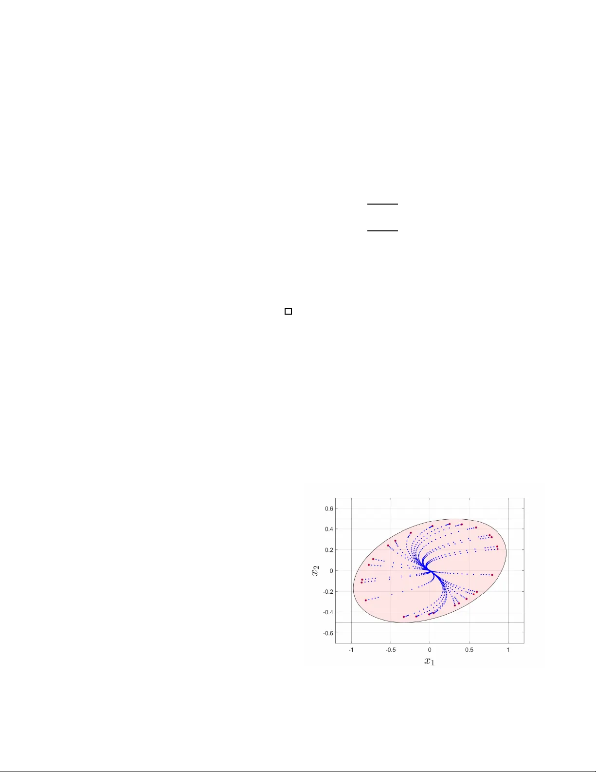
Estimation of Re gions of Attra ction for Nonlinear Systems via Coordinate-T ransformed TS Models Artun Sel Electrical and Computer Engineering The Ohio State Univ ersity Columbus, OH 43210, USA artunsel@ieee.org Mehmet K o ruturk Electrical an d Com p uter Eng ineering V irginia T ech Blacksburg, V A 2 4061 , USA mkoruturk @vt.edu Erdi Say ar Robotics, Ar tificial I ntelligence and Real- time Systems T echnical University of Mu nich Munich, Ge r many erdi.sayar@tum .de Abstract —This paper presents a novel method for estimating larger Region of Attractions (RO As) fo r continuous-t i me non- linear systems modeled via t he T akagi-Sugeno (TS) framework. While cl assical approaches rely on a single TS representation derive d from the original n onlinear system to compute an RO A using L yapunov-based analysis, th e proposed meth od enh an ces this process thro ugh a system atic coordinate transfo rmation strategy . Specifically , we construct multiple TS models, each ob- tained fro m the original n onlinear system under a distinct li n ear coordinate transfo rmation. Each transf ormed system yields a local R O A estimate, and the ov erall R O A is taken as the union of these i ndividual estimates. Th is strategy leverag es th e variability introduced by th e transformations to r educe conservatism and ex- pand the certified stable re gion. Numerical examples demonstrate that thi s app roach consisten tly provides larger RO As compared to con ventional single-model TS-b ased techniques, highlighting its effective ness and potential f or improv ed nonlinear stabili t y analysis. Index T erms —TS models, R O A, coordinate transformation, nonlinear stability , L i near Matrix Ineq uality (LMI). I . I N T RO D U C T I O N The analy sis and con tr ol of non linear systems remains a fund amental challenge in modern control theory [1]–[3] . Especially with th e rec ent developments in autonom ous aer ial vehicles with their applications in remo te sensing [4] and cyber security issues in com munication s [5]–[1 0] and energy systems [1 1]–[1 6 ], the saf ety co nsideration s are becoming more relev ant. Addition ally , the stability conc e r ns may ap p ear in co mputation al mo dels [1 7]–[2 0] and optimization algo- rithms [21]– [27] that are especially importan t in estimation problem s related to aer ospace ind ustry [28 ]–[31 ]. Am ong various m e thodolo g ies developed to add ress this, the TS fuzzy modeling framework ha s proven to be particu larly effecti ve. I t provides a systematic way to app roximate nonlinear dynamical systems throug h a con vex co m bination of linear submodels, enabling the application of p owerful LMI tech niques for controller d esign an d stability verification. When constructed via the sector nonlin e arity a p proach , TS mode ls p reserve local equiv alence to the origina l non linear dyn amics within a specified comp act doma in , makin g them a pr actical too l fo r analyzing local stability pr operties [32 ]. A key application of TS modeling lies in th e estimation of the R O A around an eq uilibrium point, often the origin. T r aditional TS- based stability analysis typically inv o lves con- structing a single TS model of the nonline a r system and verifying local or g lobal stability condition s u sing a commo n L yapun ov fu nction. These methods, while comp utationally tractable, often yield co nservati ve R O A estimates due to their reliance on a fixed co ordina te representation and restrictive L yapun ov structur es [33 ]. T o mitigate these limitations, various enhan cements hav e been proposed , such as the use of nonqu a d ratic L yap unov function s, piece wise or par ameter-dependen t f unctions, and membersh ip -functio n-dependent relaxations. Howe ver , the p o- tential of explo iting multiple coor dinate representations of the sy stem to enrich the stab ility analysis rem ains largely unexplored [34] . In th is work, we introd uce a novel approa ch to expa n d the estimated R OA by systematically transformin g th e origina l system through a family of linear coordinate changes. Each transform ed system yields a distinct T S mo d el, and an indi- vidual R OA is comp uted via standard LMI-b ased techniq u es. The final RO A is th en obtain ed as the union of these individual estimates. This fr a mew ork leverages the structu ral variation introdu c ed by coo r dinate tran sformation s to redu ce the con - servati veness inhe r ent in single-m o del metho d s [35], [ 3 6]. W e de m onstrate th rough a re p resentative example th at o ur method p roduc es significantly larger RO A estimates c ompared to conventional a pproach es, while preserving compu ta tio nal tractability . The proposed method offers a prom ising dir e ction for extend ing the applicab ility and effectiveness of TS-based stability ana ly sis fo r no nlinear systems. The r est o f the pap er is organized as follows: Section II introdu c es th e prelimin aries. Section I I I reviews the standar d TS mod eling and R OA co m putation framework. Section IV presents the pr oposed m ethod based o n coordin ate tran sfor- mation an d R OA union. Section V co ncludes the paper and discusses f uture dir e c tions. I I . P R E L I M I N A R I E S T ab le I summarize s the mathematical notation used thro ugh- out th is pa per for quick refer ence. T ABLE I M AT H E M A T I C A L N O TA T I O N Symbol Descripti on R n n -dimensiona l Euclidean s pace R m × n Set of all m × n real matric es S n Space of n × n symmetric matrices S n + Cone of n × n symmetric posi ti ve semidefinite matrice s S n ++ Cone of n × n symmetric positi ve definite matrices X  0 Matrix X is positi ve s emidefinit e X ≻ 0 Matrix X is positi ve definite X  Y Matrix X − Y is positi ve semidefinite tr ( X ) Tra ce of matrix X (sum of diagona l elements) det ( X ) Dete rminant of matrix X diag ( X ) diagona l of matrix X X ⊤ Tra nspose of matrix X x ⊤ Tra nspose of vec tor x A ⊗ B Kronecker product of m atrice s A and B h A, B i Inn er product of matrices, defined as tr ( A ⊤ B ) λ i ( X ) The i -th eigen v alue of matrix X v ( P ) Optimal valu e of optimizati on problem ( P ) con v ( S ) Con vex hull of set S h X i s X + X ⊤ A. Definitions for Mathematica l Op timization Related Con- cepts 1) Linear Matrix Inequality : An LMI is a c o nstraint of the form: F ( x ) = F 0 + m X i =1 x i F i  0 (1) where x = ( x 1 , x 2 , . . . , x m ) is th e variable vector, the sym- metric m atrices F 0 , F 1 , . . . , F m ∈ R n × n are g iven, an d the inequality symb ol  0 den otes p ositiv e semidefiniteness. An LMI defines a con vex constraint on x . Multiple LMIs can be expressed as a single LMI using blo c k -diago n al struc ture. LMIs are ce ntral to semidefinite pr o grammin g, where they serve as constrain ts in conv ex op tim ization problem s that can be solved efficiently using interior-point metho ds [37]. 2) Semi Definite Programming : Semidefinite Program- ming (SDP) is a p owerful op timization framework th at extends linear pro grammin g to th e con e of Positive Semidefinite (PSD) matrices. Forma lly , a n SDP can be expressed as: minimize h C, X i subject to h A i , X i ≤ b i , i = 1 , 2 , . . . , m X  0 (2) where X , C, A 1 , . . . , A m are symmetric n × n m atrices, b 1 , . . . , b m are scalars, and X  0 denotes that X is PSD. The constra in t X  0 means that all eig e n values of X are non-n egati ve [38]. SDP has significant app lications in control theory , com- binatorial o ptimization, and mach ine learnin g. It gen eralizes se veral o ptimization p roblems, includin g linear and q uadratic progr amming, while remain ing solvable in polynom ial time using inter ior-point methods. W hat m akes SDP p articularly valuable is its ability to provide tight relaxatio ns for many NP-hard pro blems, often yielding hig h-quality approxim ate solutions [39]. 3) Relaxation in Mathema tical Op timization : Relaxation is a fundam ental tech nique in mathematical op timization where a com plex prob lem is appro x imated by a simp ler one that is more tr actable to solve. Formally , given an op timization problem ( P ) : ( P ) : min x ∈F f ( x ) (3) a relaxation ( R ) o f ( P ) is an other op timization pro blem: ( R ) : min x ∈F ′ g ( x ) (4) where F ⊆ F ′ and g ( x ) ≤ f ( x ) for all x ∈ F . Th e key proper ty of a relaxation is that it p rovides a lower b o und on the op timal value o f the or ig inal prob lem. That is, if v ( P ) and v ( R ) d enote the optimal values of problems ( P ) and ( R ) respectively , then v ( R ) ≤ v ( P ) . Relaxation s are par tic- ularly useful for addr essing difficult optimization problems, especially th ose that a r e non-convex or NP-hard . By replacing hard co nstraints with easier ones or ap proxim ating non-conve x objective func tio ns with co nvex o nes, relaxa tio ns transform intractable pro blems into on es that can be efficiently solved. The q uality of a relaxation is me a sured by the gap b etween th e original prob lem’ s op timal value and th e relaxation’ s optimal value—a smaller g ap indicates a tighter relaxation [ 4 0]. 4) SDP Relaxatio n : SDP relaxation is a powerful tech- nique th at tran sforms difficult op timization prob lems, partic- ularly non-co nvex q uadratic problems, into tractable SDP s. Giv en a Quad ratically Constrained Quadratic Prog ramming (QCQP) of th e for m: min x ∈ R n x ⊤ P 0 x + q 0 ⊤ x + r 0 subject to x ⊤ P i x + q i ⊤ x + r i ≤ 0 , ∀ i ∈ { 1 , 2 , . . . , m } X  0 (5) the SDP relaxation pro ceeds by intr o ducing a matrix variable X = xx ⊤ and relaxing this n on-convex equality constraint to X  xx ⊤ . By the Sch u r comp lement condition, this is equiv alent to req uiring th at:  1 x ⊤ x X   0 (6) The r esulting SDP relax ation is: min x ∈ R n ,X ∈ S n tr ( P 0 X ) + q 0 ⊤ x + r 0 subject to tr ( P i X ) + q i ⊤ x + r i ≤ 0 , ∀ i ∈ { 1 , 2 , . . . , m }  1 x ⊤ x X   0 (7) where S n denotes the space of n × n symmetric matrices [ 41]. B. Definitions for Applica tions of the Methods 1) Dynamical System : A dyn amical sy stem is a mathe m at- ical model th at describes the tem poral evolution of a physical system’ s state accor ding to a fixed rule. Formally , it co nsists of a state space X and a fu nction f : X × R → X th at specifies how the state x ( t ) ∈ X e volves over time. For con tinuous-time systems, this ev olution is ty pically describ ed by a differential equation: ˙ x ( t ) = f ( x ( t ) , t ) (8) where ˙ x ( t ) represents the der i vati ve of the state with respect to time . Dynam ical systems can b e classified as lin ear o r nonlinear, time-inv a riant o r time-varying, and auton omous or non-au tonomo us. Th e an alysis of these systems f o cuses on characterizin g their stab ility pr operties, equilibr ium points, limit cycles, and other qualitative beh aviors [4 2 ]. Remark 1 . In this study , we primarily focus on polyn omial- type n onlinear systems that ar e time- invariant. F or analysis pr oblems, we specific a lly e xamine au tonomo u s systems that possess th ese p r operties. 2) Stability Definitions : Co nsider a non linear d ynamical system described b y: ˙ x = f ( x ) , x (0) = x 0 (9) where x ∈ R n is the state vector, f : R n → R n is a locally Lipschitz f unction, and f (0) = 0 (i.e., the origin is an equilibrium point) . W e define various notion s of stability as f o llows: Definition 1 ( Sta bility in the Sense of L yapunov ) . The equilibrium p o int x = 0 is stab le in the sense of Lyapunov if, for any ǫ > 0 , ther e exists a δ > 0 such tha t: k x (0) k < δ = ⇒ k x ( t ) k < ǫ, ∀ t ≥ 0 (10) Definition 2 ( A sy mptotic Sta bility ) . The equilibrium p oint x = 0 is a symptotically stab le if it is stable in the sense of L yapunov and there exists a δ > 0 such that: k x (0) k < δ = ⇒ lim t →∞ k x ( t ) k = 0 (11) Definition 3 ( Exponential Stability ) . The equilibrium point x = 0 is exponentially stab le if there exist p ositive c o nstants α , β , a n d δ such that: k x (0) k < δ = ⇒ k x ( t ) k ≤ α k x (0) k e − β t , ∀ t ≥ 0 (12) Definition 4 ( G lobal Stability ) . A stability pr ope rty (Lya- punov , asymptotic, o r exponen tial) is said to be globa l if it holds fo r a ny initia l state x (0) ∈ R n (i.e., δ → ∞ ). Definition 5 ( Local Stability ) . A stability p r operty is sa id to be local if it h olds only for initial states within some bound ed neighbo rhood of the equilibrium (i.e., k x (0) k < δ for some finite δ > 0 ). 3) Analysis Problem in LTI systems : T he analysis prob le m in L TI systems inv olves determ ining system proper ties such as stability , perfo rmance, and robustness giv en a comp lete system description but we mainly r efer to stability in this r eport. Consider a c o ntinuou s-time L TI system : ˙ x ( t ) = Ax ( t ) (13) where x ( t ) ∈ R n is the state vecto r and A ∈ R n × n is the system matrix. The stab ility analy sis prob lem can be formu lated a s veri- fying whethe r all eig e n values o f A have negative r eal parts. Using L y apunov theory , this is e quiv a lent to deter mining whether the r e exists a p ositiv e definite matrix P such that: −h P A i s ∈ S ++ (14) This verification can be expressed as a conve x feasibility problem : find P subject to P ∈ S ++ − h P A i s ∈ S ++ (15) This fo r mulation p resents a sign ifica n t advantage: the p roblem can be transfo rmed into a LMI constraint, making it co nvex and solvable in p o lynomia l time. The framework extends naturally to o ther analysis prob lems includin g H 2 and H ∞ perfor mance assessment, input-to-state stability , and robust stability against mo del un certainties, with each c ase express- ible as a n SDP with appr o priate LMI c o nstraints. 4) Synthesis Prob lem in LTI systems : Th e synthesis p rob- lem in L TI systems in volves designing con trollers that achieve desired clo sed-loop p roperties such as stability , perf o rmance, and robustness but we m a inly r efer to the stabilizin g co ntroller design problem in this report. Consider a controllable L TI system: ˙ x ( t ) = Ax ( t ) + B u ( t ) (16) where x ( t ) ∈ R n is the state vector, u ( t ) ∈ R m is the con trol input, A ∈ R n × n is the system matrix , an d B ∈ R n × m is the input matrix. For a state f eedback control law u ( t ) = K x ( t ) , the closed - loop system bec o mes: ˙ x ( t ) = ( A + B K ) x ( t ) (17) A typical synthesis p roblem a ims to find a stabilizing feedback gain K th at minimize s a perform ance criterion, suc h as an H 2 or H ∞ norm. T his can be form ulated as: minimize Performan ce Measure ( A + B K ) subject to ( A + B K ) is stable (18) If the re is n o per forman c e criter io n to be optimized, then the resulting problem is known as stabilizing controller d esign problem and it can be g iv en b y the fo llowing feasibility problem : find ( P, K ) subject to P ∈ S ++ −h P A c i s ∈ S ++ A c = A + B K (19) While this pro blem ap pears non- conv ex d ue to the p roduct term P B K , it can be transfor med into a conve x p roblem throug h a chan ge of variables. By d efining X = P − 1 and M = K X wher e P ∈ S ++ , the stability constrain t becom es: h AX + B M i s ∈ S ++ (20) which r esults in the fo llowing pr o blem: find ( X , M ) subject to X ∈ S ++ −h AX + B M i s ∈ S ++ (21) where the ( P , K ) te r ms are given by ( X − 1 , M X − 1 ) . Remark 2. It should be noted that since P ∈ S n ++ , it is an in vertible ma trix and K ca n be compu ted after compu ting the ( X, M ) pair . 5) L yap unov Function and Stability of No nlinear Dynam- ical Systems : Theorem 1. F or (9 ) , whe r e the origin is the e q uilibrium point, If ∃ V ( x ) : D → R co ntinuou sly differ en tiable such th at V (0) = 0 , ˙ V (0) = 0 , V ( x ) > 0 , ∀ x ∈ D \ { 0 } , ˙ V ( x ) < 0 , ∀ x ∈ D \ { 0 } , then x = 0 is asymptotically stable; if, in addition, D = R n and V ( x ) is radially unb ounde d , then x = 0 is glo bally asymptotically sta b le. I f V ( x ) satisfies the constraints in Ω ⊆ D , then x = 0 is loca lly asymptotically stable an d Ω is called R O A . 6) Con vex Optimization Based Nonlinear Dyna mical Sys- tem Analysis : Definition 6. A conve x model for auto nomous systems is a set of first-or de r Or d inary Differ ential Equ ationss (ODEs) whose right-han d side ca n b e expr e ssed as a conve x su m of v ector fields (m o dels), n amely ˙ x ( t ) = r X i =1 h i ( z ) f i ( x ) (22) wher e r ∈ N repr esents the number of mo dels in the conve x sum, z ∈ R p may d e pend on the state x , time t , d isturbances or exogenous parameters, and th e non linear function s h i ( z ) , i ∈ { 1 , 2 , . . . , r } hold the conve x sum pr o perty in a comp act set C ⊆ R p , i.e.: r X i =1 h i ( z ) = 1 , 0 ≤ h i ( z ) ≤ 1 , ∀ z ∈ C . (2 3) and the spec ia l case is given by ˙ x ( t ) = r X i =1 h i ( z ) A i x ( t ) (24) Definition 7. A conve x mo del for no nauton omous systems is a set of first-or der ODEs whose right-han d side can be e x p r essed as a conve x sum of vector fields ( models), na mely ˙ x ( t ) = r X i =1 h i ( z ) f i ( x , u ) (25) wher e r ∈ N r epr esen ts the number of mod els in the conve x sum, z ∈ R p may depend on the state x , input u , time t , disturb a nces or exogenous p arameters, and the no n linear functions h i ( z ) , i ∈ { 1 , 2 , . . . , r } hold the con vex su m pr ope rty in a co mpact set C ⊆ R p , i.e.: r X i =1 h i ( z ) = 1 , 0 ≤ h i ( z ) ≤ 1 , ∀ z ∈ C . (2 6) Definition 8. The vecto r z in a co n ve x mod el (25) is kno wn as the pr emise or schedulin g vector; it is assumed to be boun ded and continu ously differ entiable in a com p act set C ⊆ R p of the schedulin g/pr emise sp a ce. Definition 9. The nonlinea r functions h i ( z ) , i ∈ { 1 , 2 , . . . , r } in a conve x mod e l (25) are known as Memb ership Function s (MFs); they hold the c on vex sum pr ope rty in a co mpact set C ⊆ R p of the scheduling space. Definition 10. I f f i ( x , u ) a r e linear , i.e., f i ( x , u ) = A i x + B i u , (25 ) is called a TS mod el [4 3]; if, in addition , z doe s n o t include the sta te x it is called a linear po lytopic model [44]; if th e TS model comes fr o m fuzzy modeling techniques it is also referr ed to as TS fuzzy mo del. Definition 1 1 . A TS mod e l is a set o f first-or der ODEs wh o se right-han d side can b e expr essed as a co n ve x sum of linea r models (kno wn as co nsequents or vertex models) via non linear functions (known as membership func tio ns, MFs) th a t hold the conve x sum pr operty [45], i.e. ˙ x ( t ) = r X i =1 h i ( z )  A i x ( t ) + B i u ( t )  , y ( t ) = r X i =1 h i ( z )  C i x ( t ) + D i u ( t )  . (27) where r ∈ N is the nu mber of vertex m o dels, x ∈ R n is the state vector , u ∈ R m is th e inp ut vector, y ∈ R q is th e output vector , z ∈ R p is the premise vector (wh ich may d epend on the state, time, or exog enous parameters and is a ssumed to be bound ed and smoo th in a compact set C ⊆ R p ), A i , B i , C i , D i , i ∈ { 1 , 2 , . . . , r } are matrices of prop er dime n sions, and the MFs h i ( z ) , i ∈ { 1 , 2 , . . . , r } hold the conve x sum pr op erty in C , g iv en by (26). Theorem 2. The origin x = 0 o f the un for ce d TS mo del (24) with δ x ( t ) = ˙ x ( t ) , t ∈ R , is asymp totically stable if there exis ts a matrix P = P ⊤ > 0 such that th e follo win g LMIs hold: P A i + A i ⊤ P < 0 , i ∈ { 1 , 2 , . . . , r } . (28) In this case, any trajectory x ( t ) starting within th e out- ermost Lyapunov level V ( x ) = x ⊤ P x ≤ k , k > 0 , in a compact set of th e state space X guaranteein g z ∈ C ⊆ R p goes a symptotically to x = 0 . Pr oof. Since P = P ⊤ > 0 , V ( x ) = x ⊤ P x is a valid L yapun ov functio n candidate; its time deriv ative alo ng the trajectories of the u nforced mo del (24) is ˙ V ( t ) = ˙ x ⊤ P x + x ⊤ P ˙ x (29) = r X i =1 h i ( z ) A i x ! ⊤ P x + x ⊤ P r X i =1 h i ( z ) A i x ! = r X i =1 h i ( z ) x ⊤  A ⊤ i P + P A i  x . (30) where the last equality made use of the pro p erty P r i =1 h i ( z ) = 1 . Since h i ( z ) ≥ 0 , i ∈ { 1 , 2 , . . . , r } , ∀ z ∈ C , no t all simultaneou sly 0, it is clear that LMIs (28 ) imply ∀ x 6 = 0 then ˙ V < 0 , which mean s V ( x ) is a valid L yapun ov function establishing asympto tic stability of x = 0 . There exists a compact set X o f th e state space with 0 ∈ X , guar anteeing z ∈ C , which means that any trajectory x ( t ) in the largest L yapun ov level with in X goes asymptotically to 0. Remark 3. If th e conve x sum pr operty holds everywher e, i.e. if z ∈ C ir r espective of x , the r esults above are glo bal, i.e. X = R n . I I I . RO A C O M P U TA T I O N U S I N G T S M E T H O D In this section, th e RO A estimation using TS metho d is described b y mea n s of an num e rical example. Consider the dy n amical system d escribed by th e following equations ˙ x 1 = − ( x 1 ) 2 − 2( x 2 ) − 2( x 1 ) ˙ x 2 = ( x 2 ) 3 − x 2 (31) where an estimate of the R OA need s to be com puted by u sing TS-conve x mo deling. Considering th e region giv en by D =  x ∈ R 2 : x 1 ∈ [ − 1 , + 1] , x 2 ∈ [ − 0 . 5 , +0 . 5]  (32) the dynam ics c a n be rewritten as  ˙ x 1 ˙ x 2  =  − x 1 − 2 − 2 0 ( x 2 ) 2 − 1)   x 1 x 2  (33) and th is can be written as ˙ x ( t ) = 1 X i 1 =0 1 X i 2 =0 w 1 i 1 ( z ) w 2 i 2 ( z )  − z i 1 1 − 2 − 2 0 z i 2 2 − 1)   x 1 x 2  = X i ∈ B 2 w i ( z ) ( A i x ( t )) = A w x ( t ) , (34) where the term s are defined as z 1 = x 1 , z 2 = ( x 2 ) 2 . (35) and a re defin ed o n the set given b y C =  z ∈ R 2 : ∃ x ∈ D s.t. z 1 = x 1 , z 2 = ( x 2 ) 2  . (36) Explicitly , the terms are written a s z 1 = 1 X i 1 =0 w 1 i 1 ( x ) z i 1 1 , z 2 = 1 X i 2 =0 w 2 i 2 ( x ) z i 2 2 . (37) where the bo undary -terms are comp uted by min x 1 ( t ) , x 2 ( t ) z 1 ( t ) = z i 1 =0 1 , max x 1 ( t ) , x 2 ( t ) z 1 ( t ) = z i 1 =1 1 , min x 1 ( t ) , x 2 ( t ) z 2 ( t ) = z i 2 =0 2 , max x 1 ( t ) , x 2 ( t ) z 2 ( t ) = z i 2 =1 2 . (38) and th e cor respond in g MFs are given by w 1 i 1 =1 ( x ) = z 1 1 − z 1 z 1 1 − z 0 1 , w 1 i 1 =0 ( x ) = 1 − w 1 i 1 =1 ( x ) . w 2 i 2 =1 ( x ) = z 1 2 − z 2 z 1 2 − z 0 2 , w 2 i 2 =0 ( x ) = 1 − w 2 i 2 =1 ( x ) . (39) Using Theo rem 2, the prob lem can be stated by the f ollowing feasibility p roblem: find P subject to P ∈ S ++ − h P A i i s ∈ S ++ , ∀ i (40) The m atrix is com p uted to be P =  0 . 2017 − 0 . 1326 − 0 . 132 6 0 . 7656  (41) and RO A is param eterized by a term, k which is compu ted by max k subject to Ω =  x ∈ D : x ⊤ P x ≤ k  Ω ⊆ D (42) and k is comp uted to be 0 . 17 using th e metho d described in [46] an d the co rrespond ing RO A is illustrated in Fig-1. Fig. 1. R OA for the system computed with the TS method I V . ROA C O M P U TA T I O N U S I N G C O M B I N E D S TA T E T R A N S F O R M AT I O N A N D T S M E T H O D For the stability analysis meth od, TS-metho d is useful in that it o ffers a straightforward algorithm to construct a L yapun ov fu n ction to g uarantee a local asym ptotical stability . Unfortu n ately , the results depen ds on the MFs and, as stated previously , that p rocess is n ot straightf orward, since there is not a un ique set of M Fs f o r a given system. Howe ver , instead of finding the ’best’ set of MFs to max imize the RO A , we can have a relatively simple ’metho d for comp uting th e set of MFs’ for a given dyna mical system and we can ge t one R OA , and then by implementin g a ch a nge of variables ¯ x = T ( x ) resulting in ˙ ¯ x = ¯ f ( ¯ x ) , and applying the same TS-method to th is system r esults in another R O A , we can compute the boun dary o f the ellipso idal region s (for example by r epresenting them as a set of points that are defined in ¯ x - space) and transfo rming th em into the x -space would give us another r egion th at is gu aranteed to b e locally asymp totically stable. Addition ally , the aforemen tioned transforma tio n for th e change o f variables can be as simple as a linear transfo rmation where T ( x ) = T x , whe r e T ∈ R n × n is a ny in vertible matrix. F or th e p r oblem stated in Section III, this ’chan ge of variables idea’ c an be impleme nted. By cho osing a simple transform ation matrix T =  1 2 0 1  (43) which r esults in the fo llowing system ˙ ¯ x 1 = − ( ¯ x 2 1 ) + 4( ¯ x 1 )( ¯ x 2 ) − 2( ¯ x 1 ) + 2( ¯ x 3 2 ) − 4( ¯ x 2 2 ) ˙ ¯ x 2 = ( ¯ x 3 2 ) − ¯ x 2 (44) and b y ch oosing the following set of MFs : z 1 = ¯ x 1 , z 2 = ¯ x 2 , z 3 = ¯ x 2 2 . (45) By c hoosing th e following region o f inter est ¯ D = { x : ¯ x 1 ∈ [ − 0 . 55 , +0 . 55 ] , ¯ x 2 ∈ [ − 0 . 55 , +0 . 55 ] } (46) and the RO A for the ¯ x -d omain an d the region that is comp uted by map ping that region b ack to th e origina l x -domain is illustrated in Fig -2. It can be seen that the red-ellipse which represents the bound aries of the e llipsoidal region that is comp uted using th e presented ’ change of variables meth od’ ha s some are a s outside of the o riginal RO A th at is com puted in the Section III an d that suggests that iteratively using a method (by auto matizing the set of MFs for a given nonlin ear d ynamical system ) results in a larger R OA. V . C O N C L U S I O N S In this study , we exp lo red the u se of SDP relaxatio ns and LMIs as powerful tools fo r analyzin g a n d designin g control systems. As a key application, we employed the TS modeling framework to study RO A estimation prob lem. The TS a p - proach ena b led us to leverage co n vex o ptimization techn iq ues to hand le no nlinear dynamics effecti vely . Furthermore , we propo sed an extension to the standard meth ods, aimed at Fig. 2. (a) RO A computed for the system whose state varia ble is ¯ x ∈ ¯ D (b) RO A computed for the s ystem whose state vari able is x ∈ D by using the TS-method illustra ted by red-shaded regi on and the boundary of the R OA that is computed in ¯ D domain and mapped to D enhancin g their applicability and reducing conservatism in practical scena rios. T hese co ntributions collectiv ely demo n- strate the p otential of combinin g TS mod eling with SDP-based tools to ad dress challeng ing problems in no n linear dynam ic a l systems. R E F E R E N C E S [1] B. Kurkcu, C. Kasnakoglu, and M. Efe, “Disturbance/ uncert ainty es- timator based inte gral sliding-mod e control, ” IEEE Tr ansactions on Automat ic Contro l , vol. 63, no. 11, pp. 3940–3947, 2018. [2] ——, “Disturbance/ uncertain ty estimator based robust control of non- minimum phase systems, ” IEEE/ASME T ransactions on Mech atr onics , vol. 23, no. 4, pp. 1941–1951, 2018. [3] B. Kurkcu and C. Kasnako glu, “Robust autopilo t desi gn based on a disturbance /uncer tainty/coupling esti mator , ” IEEE T ransac tions on Contr ol Systems T ec hnolo gy , vol. 27, no. 6, pp. 2622–2629, 2019. [4] H. Madani, M. Setti, D. Akziz, and Z. Nemer , “ Assessment of land use–land cover changes using G IS, remote sensing, and CA–Marko v model: a case study of Algiers, Algeria , ” Applied Geomatics , vol. 14, no. 4, pp. 811—-825, N ov 2022. [Online ]. A vaila ble: http:/ /dx.doi.or g/10.1007/ s12518-022-00472-w [5] A. Etcibasi and E. Aktas, “Co vera ge analysis of IRS-aided m illimet er- wa ve netwo rks: A practica l approach, ” IEEE T ransactions on W irel ess Communicat ions , vol. 23, no. 4, pp. 3721–3734, 2024. [6] A. Mohammadi, R. Ahmari, V . Hemmati, F . Owusu-Ambrose, M. Mah- moud, P . Kebria , and A. Homaif ar , “Detect ion of multiple small biased GPS spoofing attacks on autonomous veh icles using time series analy- sis, ” IEEE Open J ournal of V ehicular T ech nolo gy , v ol. 6, pp. 1152–1163, 2025. [7] A. Mohammadi, V . Hemmati, R. Ahmari, F . Owusu-Ambrose, M. Mah- moud, and A. Homaifar , “GPS spoofing atta ck detect ion on autonomous vehi cles using modified DBSCAN with dynamic thre shold, ” in P r oceed- ings of the 5th IFSA W inter Confer ence on Automation, Robotics & Communicat ions for Industry 4.0/5.0 (A RCI’2025) , 2025, pp. 74–76. [8] ——, “Detection of multiple sm all biased GPS spoofing attacks on autonomous vehicle s, ” in 2025 IEEE 4th International Confer ence on AI in Cyber securit y (ICAIC) . IEEE , 2025, pp. 1–9. [9] R. Ahmari, V . Hemmati, A. Mohammadi, P . Kebria , M. Mahmoud, and A. Homaifar , “ A data-dri ven approac h for UA V -UGV inte gration, ” Pro - ceedi ngs of the Automati on, Robotics & Communications for Industry , vol. 4, no. 5. 0, p. 77, 2025. [10] R. Ahmari, V . Hemmati, A. Mohammadi, M. Mynuddin, P . Kebria , M. Mahmoud, an d A. Homaifar , “Eva luati ng trojan attack vul nerabil itie s in autonomous landing systems for urban air mobility , ” Pr oceedings of the Automation , Robotics & Communications for Industry , vol. 4, no. 5.0, p. 80, 2025. [11] N. Agrawa l, “Performance of con ventiona l and modified solar photo volt aic array configurat ion under the combined ef fect of seasonal v ariati on and partial shaded conditions, ” Journal of Energy Systems , vol. 9, no. 1, pp. 52—-67, Mar 2025. [Online]. A v aila ble: http:/ /dx.doi.or g/10.30521 /jes.1523575 [12] F . Himmelstoss and H. V otzi, “Floating double boost con vert er , ” J ournal of Energ y Systems , vol. 9, no. 1, pp. 85—-104, Mar 2025. [Online]. A vail able: http:/ /dx.doi.or g/10.30521/jes.1525077 [13] D. K och, P . Balv e, J. Gerdes, M. Hertwig, M. M. Kroll, and J. Lentes, “Qualitati ve and quantitati ve analysis of ultra -ef ficiency project s: Commonalities, dif ferenc es, and lessons learned, ” J ournal of Ener gy Syst ems , vol. 9 , no. 1, pp. 68—-84, Mar 2025. [Onli ne]. A v aila ble: http://dx.doi.or g/10.30521/jes.1524221 [14] M. Albasheri, O. Bouchhida, Y . Soufi, A. Cheri fi, A. Muj ammal, and A. Moualdia, “Energy management techni que of hybrid ener gy storage system-based DC microgrid, ” Journal of Energy Systems , vol. 9, no. 1, pp. 36––51, Mar 2025. [Online]. A vaila ble: http:/ /dx.doi.or g/10.30521 /jes.1523522 [15] R. Ekawita , I. Almadi, and E. Y uliza, “In vest igati ng rooftop solar energy potenti al in coastal area with unmanned aerial vehicl e technolo gy , ” J ournal of Ener gy Systems , vol . 9, no. 1, pp. 1—-11, Mar 2025. [Online]. A vail able: http:/ /dx.doi.or g/10.30521/jes.1416277 [16] L. Pham, C. Kutay , and G. James, “Potentia l for a circula r economy for sustainab le large -scale rene wable energy systems, ” Journal of E ner gy Systems , vol. 9, no. 2, pp. 172––185, May 2025. [Online]. A vail able: http:/ /dx.doi.or g/10.30521 /jes.1518827 [17] B. S el, R. Jia, and M. Jin, “LL Ms can plan only if we tell them, ” in Pr oceed ings of International Confer ence on Learning Repr esentat ions ICLR , 2025. [18] M. Jin, B. Sel, F . Hard eep, and W . Y in, “Democra tizi ng energy manage- ment with LLM-assisted optimizat ion autoformal ism, ” in Procee dings of 2024 IEEE Internati onal Confer ence on Communicat ions, Contr ol, and Computing T ec hnolo gies for Smart Grids (SmartGridComm) , 2024, pp. 258–263. [19] B. Sel, P . Shanmugasundara m, M. Kachuee, K. Zhou, R. Jia, and M. Jin, “Skin-in -the-game : Decision making via multi-stak eholder alignment in LLMs, ” in Pr oceedi ngs of the 62nd Annual Meeting of the Association for Computati onal Linguistics (ACL) (V olume 1: Long P apers) . Asso- ciati on for Computational Linguistics, Aug 2024, pp. 13 921–13 959. [20] B. Sel, A. Al-T awaha , V . Khattar , R. Jia, and M. Jin, “ Algorithm of thoughts: enhanc ing explorat ion of ideas in large language models, ” in Pr oceed ings of the 41st International Confer ence on Machine L earning (ICML) , ser . ICML ’24, 2024. [21] S. G u, B. Sel, Y . Ding, L. W ang, Q. Lin, A. Knoll, and M. Jin, “Safe and balanced: A framewor k for constrained multi-object i ve reinforce - ment learning, ” IEEE T ransactio ns on P attern A nalysis and Machine Intell ige nce , vol. 47, no. 5, pp. 3322–3331, 2025. [22] S. Gu, B. Sel, Y . Ding, L. W ang, Q. Lin, M. Jin, and A. Knoll, “Bala nce re ward and safety optimization for s afe reinforcement le arning: A perspecti ve of gradient manipulatio n, ” vol. 38, no. 19. Association for the Adva ncement of Artificial Intellige nce (AAAI), Mar 2024, pp. 21 099––21 106. [23] M. Jin, V . Khat tar , H. Kaushik, B. Sel, and R. Jia, “On solution funct ions of optimizatio n: Univ ersal approx imation and cove ring number bounds, ” in Pr oceed ings of the AA AI Confere nce on Ar tifici al Intellige nce , vol. 37, no. 7. Associati on for the Advanc ement of Artificial Intelligen ce (AAAI), Jun 2023, pp. 8123—-813 1. [24] B. Sel, A. T awa ha, Y . Ding, R. Jia, B. Ji, J. Lava ei, and M. Jin, “Learning -to-lea rn to guide random search: Deriv ati ve -free meta blackbo x optimiz ation on manifold, ” in P r oceedings of T he 5th Annual Learning for Dynamics and Contr ol Confere nce , ser . Proceed ings of Machine Learning Research, vol. 211. PMLR, Jun 2023, pp. 38–50. [Online]. A vail able: https:/ /proce edings.mlr .press/v211/sel23a.html [25] A. T aw aha, H. Kaushik, B. Sel, R. Jia, and M. Jin, “Decision-focuse d learni ng for in verse noncoope rati ve games: Genera lizat ion bounds and con ver gence analysis, ” IF AC-P apersOnLi ne , vol. 56, no. 2, pp. 9336–9341, 2023, 22nd IF A C W orld Congress. [Online]. A va ilabl e: https:/ /www .sciencedi rect.com/science/article/pii/S2405896323005724 [26] V . Khatt ar , Y . Ding, B. Sel, J. Lava ei, and M. Jin, “ A CMDP-within-online framew ork for meta-safe reinforcemen t learning, ” in Proce edings of Internationa l Confe re nce on Learning Repr esentations (ICLR) 2023 , 2023, published on OpenRe view and arXiv . [Online]. A v aila ble: https://a rxi v .org/ abs/2405.16601 [27] U. Coskun, B. Sel, and B. Plaster , “Magnetic field mapping of inaccessi ble regions using physics-informed neural netwo rks, ” Scient ific Reports , vol. 12, no. 1, Jul 2022. [Online]. A v ailable: http:/ /dx.doi.or g/10.1038/ s41598-022-15777-4 [28] S. Pourtakdoust, M. Mehrjardi , M. Hajkarim, and F . Nasihat i, “ Advan ced faul t detect ion and diagnosis in spacecra ft attitude control systems: Cur- rent state and challenges, ” Pr oceedings of the Institution of Mec hanical Engineer s, P art G: Journal of Aer ospace Engineering , vol. 237, no. 12, pp. 2679–2699, 2023. [29] F . Nasihati , M. Kiani, and S. Pourtakdo ust, “Satell ite pose estimati on using earth radiation modeled by artificia l neural networks, ” Advances in Space Resear ch , vol. 70, no. 8, pp. 2195–2207, 2022. [30] —— , “On-line orbit and albedo estimation using a strong tracking algorit hm via satellit e surface temperature data, ” IEEE T ransacti ons on Aer ospace and E lectr onic Systems , vol. 57, no. 3, pp. 1443–145 4, 2021. [31] —— , “ Autonomous tempe rature-b ased orbit estimati on, ” Aer ospace Scienc e and T echnol ogy , vol. 86, pp. 671–682, 2019. [32] T . Guerra, R. M ´ arquez, A. K ruszewski, and M. Bernal, “ h ∞ lmi-based observe r design for nonline ar systems via takagi–suge no m odels with unmeasured premise variab les, ” IEEE T ransac tions on Fuzzy Systems , vol. 26, no. 3, pp. 1498–1509, 2018. [33] F . L ´ opez-Estra da, H. H. de Le ´ on, V . Estrada-Manzo , and M. Bernal, “Lmi-based fault detecti on and isolation of nonlinear descriptor sys- tems, ” in Pr oceedings of IEEE International Confe re nce on Fuzzy Systems , 2017, pp. 1–5. [34] M. Della Rossa, A. T anwan i, and L. Zaccarian, “Max–min lyapunov functio ns for switch ed systems an d rela ted dif ferential inclusions, ” Automat ica , vol . 120, p. 109123, 2020. [35] F . Sotiropoulos and H. Asada, “Causality in dual face ted linearizat ion of nonline ar dynamical systems, ” in 2018 Annual American Contr ol Confer ence (ACC) , 2018, pp. 1230–1237. [36] Y . Igara shi, M. Y amakita, J. Ng, and H. Asada, “ A robust method for dual fa cete d lineariz ation, ” IF A C-P apersOnLine , vol. 53, no. 2, pp. 6095––61 00, 2020. [Online ]. A vai lable : http:/ /dx.doi.or g/10.1016/ j.ifacol.2020.12.1683 [37] S. P . Boyd and L. V anden bergh e, Con ve x optimization . Cambridge uni versity press, 2004. [38] R. T edrak e, I. R. Manchester , M. T obenkin, and J. W . Roberts, “Lqr-tre es: Fe edback motion planning via sums-of-squa res veri ficatio n, ” The Internationa l J ournal of Robotics R esear ch , vol. 29, no. 8, pp. 1038––1052, Apr . 2010. [Online] . A v ailable: http:/ /dx.doi.or g/10.1177/ 0278364910369189 [39] B. Recht, M. Faz el, and P . A. Parrilo, “Guaranteed minimum-rank solutions of linear matrix equati ons via nuclear norm minimizat ion, ” SIAM R evi ew , vol. 52, no. 3, pp. 471—-501, Jan. 2010. [Online]. A v aila ble: http:// dx.doi.org /10.1137/07 0697835 [40] A. Nedic, A. Ozdaglar , and P . Parril o, “Constraine d consensus and optimiza tion in m ulti-a gent networks, ” IEEE T ransaction s on Automat ic Contr ol , vol. 55, no. 4, pp. 922–938, 2010. [41] S. Kuindersma, F . Permenter , and R. T edrake, “ An effic ientl y solvabl e quadrat ic program for stabiliz ing dynamic locomotion, ” in 2014 IEEE Internati onal Confer ence on Robotics and Automation (ICRA ) , 2014, pp. 2589–2594. [42] G.-R. Duan and H. -H. Y u, LMIs in Contr ol Systems . CRC Press, Jun. 2013. [Online]. A v aila ble: http://d x.doi.org/ 10.1201/b1 5060 [43] M. Bernal , A. Sala, Z. Lendek, and T . M. Guerra , Analysis and s ynthesi s of nonlinear con tr ol systems , 2022nd ed., ser . Studies in systems, decisio n and control . Cham, Switzerla nd: Springer Nature, Feb . 2022. [44] T . T akagi and M. Sugeno, “Fuzzy identifica tion of systems and its applic ations to modeling and control , ” IEEE T rans. Syst. Man Cybern. , vol. SMC-15, no. 1, pp. 116–132, Jan. 1985. [45] K. T anaka and H. O. W ang, Fuzzy contr ol systems design and analysis , ser . W iley-In terscie nce publica tion. Nashville, TN: John W iley & Sons, Jul. 2001. [46] R. Robles, A. Sala, M. Bernal, and T . Gonz ´ alez, “Subspace-based takagi –sugeno modeling for improved lmi performance , ” IEEE T rans- actions on Fuzzy Systems , vol. 25, no. 4, pp. 754–767, 2017.