Optimal Switching in Networked Control Systems: Finite Horizon

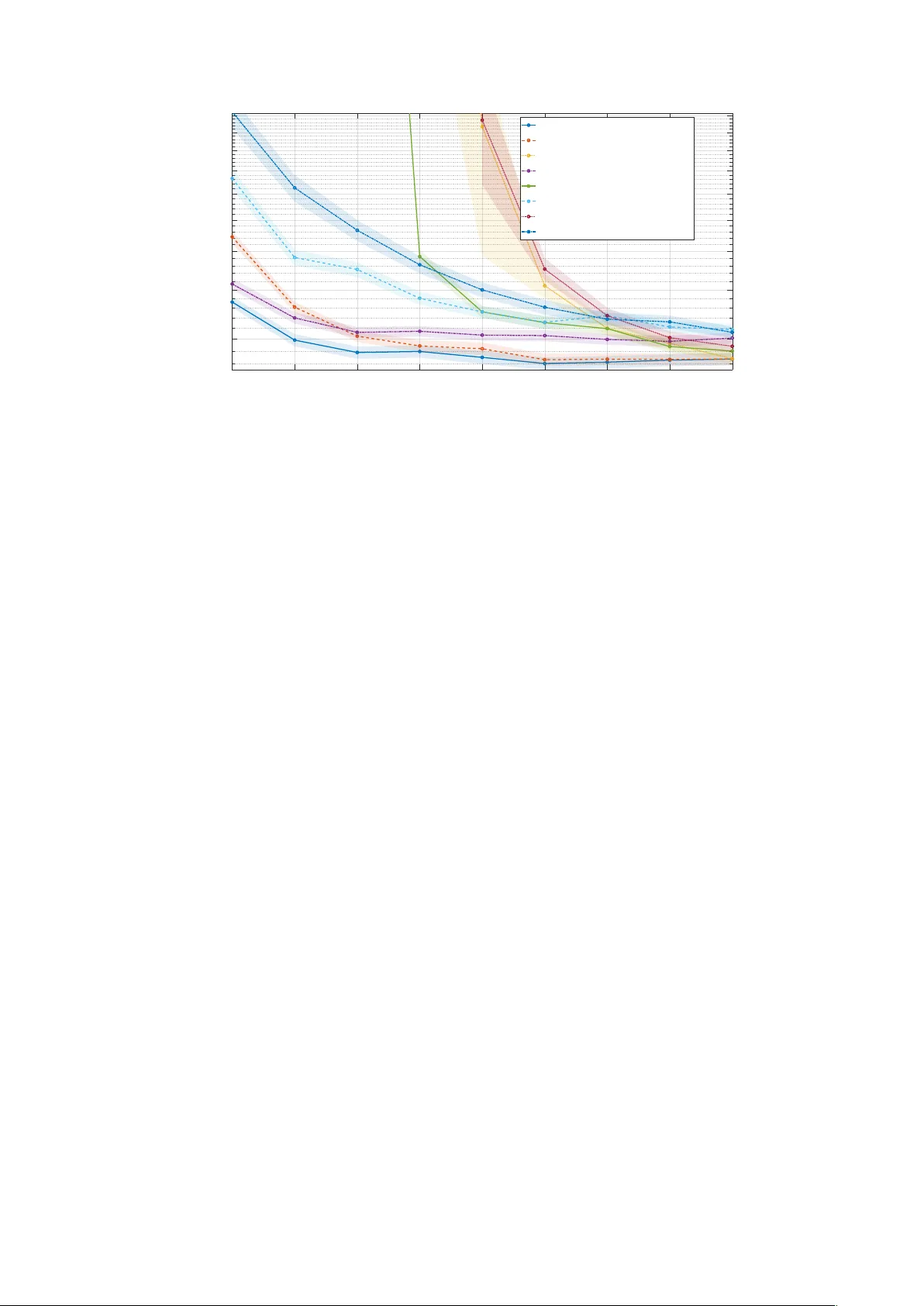
Optimal Switc hing in Net w ork ed Con trol Systems: Finite Horizon Ab dullah Y asin Etcibasi, C. Emre Koksal, and Eylem Ekici The Ohio State Univ ersity { etcibasi.1, koksal.2, ekici.2 } @osu.edu 1 Abstract In this w ork, we ﬁrst pro v e that the separation principle holds for switched LQR problems under i.i.d. zero-mean disturbances with a symmetric distribution. W e then solv e the dynamic programming problem and sho w that the optimal switc hing policy is a symmetric threshold rule on the accum ulated disturbance since the most recen t up date, while the optimal controller is a discoun ted linear feedback law independent of the switc hing p olicy . 2 In tro duction Ov er the past three decades, wireless communication has adv anced rapidly . Starting with early generations, esp ecially 4G, wireless connectivity became an essential part of daily life. With the adv ent of 5G and the forthcoming 6G, we are now entering a new “rob otic era,” characterized b y p erv asiv e autonomous agents suc h as rob ot v acuums, self-driving v ehicles, and aerial drones. Unlik e previous eras, these agents m ust not only comm unicate with humans but also co ordinate among themselv es, forming sw arms of drones and platoons of v ehicles. Consequen tly , engineers m ust join tly address comm unication and con trol, rather than treat these domains indep enden tly . T raditionally , wireless system designers hav e tended to ignore control lo op requiremen ts, while control engineers hav e assumed p erfect communication channels [1]. In practice, con trol strategies m ust tolerate netw ork imperfections, and comm unication proto cols should resp ect the dynamics of the underlying physical systems [2]. This in terplay has given rise to the ﬁeld of net work ed con trol systems (NCSs) [3, 4]. As the name suggests, NCS researc h inv estigates con trol lo ops in which one or more feed- bac k paths trav erse a comm unication net w ork. Early contributions introduced pac k et losses and delays into feedbac k con trol and examined the resulting p erformance and stabilit y . F or example, ˚ Astr¨ om and Bernhardsson compared the mean v ariance of a contin uous-time system under p eriodic sampling and state-dep endent (even t-triggered) sampling, assuming impulsiv e con trol actions at sampling instan ts [5]. T abuada prop osed an even t-triggered feedback p olicy 1 for linear time-in v arian t (L TI) systems, where the maximum update p erio d dep ends on the estimation error; the controller emplo ys a zero-order hold (ZOH), up dating only at sampling times and holding the con trol v alue constant in b etw een [6]. Mon testruque and Antsaklis in- v estigated the sto chastic stabilit y of NCSs with time-v arying up date in terv als (indep endent and identically distributed (i.i.d.) or Mark ov-c hain driv en) modeling the sampled system as a jump-linear system [7]. Heemels et al. introduced self-triggered sampling, where eac h up- date time is computed at the preceding up date and compared with even t-triggered policies [8]. Zhang et al. separately examined the eﬀects of delays and pack et drop outs on stabilit y . Dela ys w ere handled b y employing system estimates in b oth full-state and partial-state feedback, while pac ket dropouts w ere analyzed under p erio dic transmissions to determine the minimum stable transmission rate [3]. Finally , Lyapuno v-based analyses by Heemels and colleagues established the maximum allow able transmission interv al (MA TI) and maximum allow able delay (MAD) that ensure NCS stabilit y [9]. F undamentally , any NCS consists of t wo k ey design comp onen ts. These are the switching 1 mec hanism and the controller (see Fig. 1). In this work, w e fo cus on their join t optimization. W e mo del system uncertain ties as i.i.d. zero-mean disturbances with a symmetric distribution and emplo y a standard quadratic cost on state deviations and con trol eﬀort. This form ulation is kno wn as the Linear Quadratic Regulator (LQR), since the ob jectiv e is to regulate the system state to the origin. This criterion is widely used in the NCS literature [1]. Our aim is to ﬁnd the optimal switc hing and control p olicies for the ﬁnite-horizon LQR problem under an av erage switc hing-rate constraint. The main diﬃculty arises from the dual eﬀect, whereb y transmission decisions inﬂuence future estimation errors while con trol actions aﬀect the evolution of the estimator. This coupling b etw een the switc hing mec hanism and the con troller breaks the classical separation principle, whic h ordinarily allows the estimator and con troller to b e designed indep endently without loss of optimality [10]. T o regain separability , m uch of the existing literature imp oses simplifying assumptions, most commonly b y restricting atten tion to a sub class of p olicies under whic h the conditional mean of the accumulated dis- turbance is zero. W e deﬁne such p olicies as symmetric p olicies . While this assumption renders the problem analytically tractable, it restricts the p olicy space, raising the question of whether this sub class is optimal. Crucially , how ev er, the optimality of this restricted p olicy space has y et to b e pro ven, represen ting a signiﬁcant gap in the current understanding of switched LQR problems. In what follo ws, w e review ho w this join t optimization problem has b een treated in the literature, highlighting the widespread use of the symmetry ass umption, sometimes im- p osed explicitly b y assuming zero-mean disturbances and sometimes adopted implicitly through Bernoulli sampling mo dels, or symmetric threshold rules. In [11], the switc hing-rate constraint was relaxed through a Lagrangian formulation, and separation was enforced b y assuming zero-mean disturbances. The design was then recast as an equiv alen t optimal-estimation problem to enable n umerical solutions. An equiv alen t form of the symmetry assumption w as adopted implicitly in [12], where the design was reformulated as 1 In the literature, this mechanism is referred to by v arious terms suc h as scheduling, sampling, transmission, or switching. Throughout this pap er, we adopt the term switching . 2 an age-of-information (AoI) minimization problem and a heuristic sc heduler was prop osed. In a t wo-hop multi-system setting [13], disturbances w ere likewise constrained to b e zero-mean, and AoI- and v alue-of-information (V oI)-based sc hedulers were compared numerically . Building on this line of w ork, a V oI metric w as in tro duced in [14], for whic h a threshold p olicy w as proposed, and the concept w as further reﬁned in [15] with corresp onding sampling thresholds. An alternativ e line of w ork was pursued in [16], where sampler up dates were mo deled as i.i.d. Bernoulli even ts. It w as shown that a linear state-feedback law, with gain given by the Riccati solution, remains optimal under random pack et drops, and the resulting stability w as analyzed. Similarly , link failures were treated as Bernoulli losses in [17], where an impulsive con troller (no con trol when the link fails) w as implemen ted, again reco vering the linear feedbac k con troller as LQG-optimal. Other studies ha ve fo cused on the join t switc h and controller design under symmetric thresh- old p olicies. In [18], a threshold w as imp osed on the squared estimation error, under which the linear feedback la w was found to b e optimal. The relation b etw een this threshold and the Lagrange m ultiplier w as inv estigated in [19], with con vergence and stabilit y prop erties ana- lyzed. Energy constrain ts at the sensor were incorporated in [20], where a threshold based on the conditional co v ariance of the estimation error was proposed. More recen t w ork [21] emplo yed a Q-learning–based reinforcement-learning algorithm under the same symmetric as- sumption, while v arying delays w ere addressed in [22] through a mixed-in teger control problem solv ed oﬄine with Riccati metho ds and integer programming. F rom a diﬀeren tial-game p er- sp ectiv e [23], contin uous and intermitten t sensing play ers w ere contrasted, leading to AoI-based threshold rules. Finally , the disturbance-driv en estimation dynamics w ere correctly modeled in [24], where a relaxed dynamic program for the sampler w as formulated and an approximate solution prop osed due to computational complexit y . In this w ork, we make the follo wing contributions: • W e revisit the constrained join t design of switc hing and con trol policies for scalar L TI systems, aiming to clarify subtle underlying assumptions. • Most imp ortan tly , we pro ve that symmetric p olicies are optimal for the ﬁnite-horizon switc hed LQR problem under a switc hing-rate constrain t, thereby establishing that the separation principle holds. • Finally , we solve the asso ciated dynamic programming (DP) problem and derive the op- timal switc hing and con trol p olicies, whic h take the form of a symmetric threshold rule on the estimation error and a discounted linear feedback la w that is indep enden t of the switc hing p olicy , resp ectively . W e b egin b y analyzing the information structure of the system and iden tifying when the classical separation principle breaks down. W e then discuss why at least a unit-dela y must b e in tro duced b et ween switch and controller. Then, w e in tro duce the class of symmetric p olicies and demonstrate that under these policies, the dual eﬀect is neutralized, allowing the estimation and con trol tasks to decouple. W e rigorously prov e that this sub class is not only tractable but 3 Figure 1: Block diagram of the closed-lo op con trol system optimal for the ﬁnite-horizon LQR problem under a switching-rate constraint. Finally , w e deriv e the closed-form solution for the optimal system, which consists of a linear feedback con trol la w and a symmetric threshold switchi ng p olicy based on the accum ulated disturbances. 3 System Mo del Consider the single-lo op, discrete-time, scalar L TI system illustrated in Fig. 1. The plant P ev olves according to X k +1 = aX k + bU k + W k , (1) where X k denotes the system state, U k the control input, and W k an additive disturbance. The disturbance sequence { W k } is assumed to b e i.i.d., zero-mean, with ﬁnite v ariance σ 2 W , and symmetric around zero. The controller receives intermitten t information through a switch with a ﬁxed τ ≥ 1 delay , so that the observ ation av ailable to the controller is Y k = D k − τ X k − τ , (2) where D k ∈ { 0 , 1 } denotes the switching decision at time k . In the sequel, we discuss why at least a one-step dela y must b e introduced b et ween the switch and the controller. Let t k denote the most recen t switching time prior to k , deﬁned as t k := max { j ≤ k | D j = 1 } . The con troller’s information at time k is giv en by I C k = { Y 0 , U 0 , Y 1 , U 1 , . . . , Y k − 1 , U k − 1 , Y k } . (3) The information v ector at the switc h plays a k ey role in the optimal-switc hing problem. V arious approac hes and information sets app ear in the literature. In the most general form, we denote the switc h’s information by I S k = { X 0 , D 0 , U 0 , X 1 , D 1 , U 1 , . . . , X k − 1 , D k − 1 , U k − 1 , X k } . (4) Remark 1. Under delay-fr e e fe e db ack, the c ontr ol ler information set includes Y k = D k X k ∈ I C k . 4 Note that Y k dep ends explicitly on the switching de cision D k . However, at time k , the switch only has ac c ess to D k − 1 ∈ I S k . Sinc e the c ontr ol ler is lo c ate d downstr e am of the switch, including Y k = D k X k in the c ontr ol ler information set violates c ausality [25]. Ther efor e, at le ast a one-step delay must b e intr o duc e d b etwe en the switch and the c ontr ol ler to ensur e a c ausal information structur e. Note that several works in the literature assume delay-free feedback and study separation or optimal switc hing in the switched LQR problem [11, 13, 18–20, 26–28]. How ev er, as sho wn in Remark 1, suc h formulations are non-causal, rendering the asso ciated DP recursion ill-p osed. The con trol and switching p olicies are deﬁned as U k = γ k  I C k  ∈ Γ , (5) D k = f k  I S k  ∈ Π , (6) where the sets Γ and Π contain all admissible con trol and switching decision rules that satisfy the usual measurability and integrabilit y conditions. W e write µ = ( γ 0 , γ 1 , . . . ) ∈ Γ and π = ( f 0 , f 1 , . . . ) ∈ Π for generic control- and switching-policy sequences, resp ectively . Because the t wo sequences are designed jointly , µ and π can b e coupled. The main ob jectiv e is to minimize constrained exp ected LQR cost ov er a ﬁnite horizon P 1 : min π ∈ Π , µ ∈ Γ 1 N E " N − 1 X k =0  q X 2 k + r U 2 k  + X 2 N # (7) s.t. 1 N N − 1 X k =0 D k ≤ r s (8) where q , r, r s > 0. Theorem 1. Consider the system (1) – (4) and the optimization pr oblem P 1 . The optimal c ontr ol ler is given by the line ar fe e db ack law 2 U k = γ k ( I C k ) = − L ˆ X k , (9) wher e ˆ X k = E  X k | I C k  , L = ab P r + b 2 P , P = a 2 P + q − ( abP ) 2 r + b 2 P . (10) Pr o of. See App endix A. Let us deﬁne the estimation error at the controller as E k = X k − ˆ X k . (11) Giv en the optimal con troller in (9), the ob jective function in (7) can b e reformulated in terms of the estimation error E k . The goal is then to determine the optimal switching p olicy that minimizes this reform ulated cost. 2 W e assume a suﬃciently large horizon length so that the steady-state Riccati solution is applicable. The extension to the transient case is straightforw ard. 5 Theorem 2. F or a sc alar L TI system with q , r > 0 , a ﬁxe d delay τ ≥ 1 , and using the optimal c ontr ol ler in (9) , pr oblem P 1 c an b e e quivalently written as P 2 : min π ∈ Π 1 N E " N − 1 X k =0 E 2 k # (12) s.t. 1 N N − 1 X k =0 D k ≤ r s . Pr o of. See App endix B. In formulation P 2 , the cost dep ends only on the estimation error. Consequen tly , if the estimation-error dynamics can b e written indep endently of the control inputs, the control and switc hing problems decouple, i.e., the separation principle holds. Note that without the sep- aration principle, although Theorem 1 giv es the optimal control la w U k = − L ˆ X k , the state estimate ˆ X k itself dep ends on the switc hing p olicy π . Until π is ﬁxed, the estimator remains undeﬁned and the closed-lo op law cannot b e completed. Only once π is chosen can b oth the estimator and the corresp onding optimal con troller b e fully sp eciﬁed. 4 Symmetric P olicies In this section, we b egin by deriving the estimation error dynamics to identify the precise conditions under which the separation principle remains v alid. Within this framework, we formally deﬁne the class of symmetric p olicies, a sub class c haracterized b y the prop ert y that the accum ulated disturbance remains conditionally zero-mean with resp ect to the controller’s information. While suc h p olicies are often treated as a mere mo deling conv enience, they hav e silen tly shap ed muc h of the literature in even t-triggered con trol, frequently appearing as hidden or unstated assumptions. W e demonstrate that the statistical coupling b etw een switc hing decisions and disturbances fundamen tally preven ts estimation error decoupling unless this symmetry is imp osed. Ulti- mately , this section provides the necessary foundation for Section 5, where we mo ve beyond tractabilit y to rigorously prov e that these symmetric p olicies are, in fact, optimal. 4.1 Estimation Error Dynamics and the Role of Symmetry The analysis b egins b y deriving the estimation error dynamics based on the controller’s av ailable information, setting the stage for examining the v alidity of the separation principle. Lemma 1. Consider the system (1) – (2) under the information structur es (3) – (4) . Then the estimation err or dynamics ar e given as fol lows: 6 E k +1 = (1 − D k +1 − τ )  a  X k − E [ X k | I C k , D k +1 − τ = 0]  + W k  + D k +1 − τ   τ − 1 X j =0 a τ − 1 − j W k +1 − τ + j   . (13) Pr o of. F or τ ≥ 1 and the switching instant t k , w e obtain E t k + τ = a τ  X t k − E [ X t k | I C t k + τ ]  + τ − 1 X j =0 a τ − 1 − j  W t k + j − E [ W t k + j | I C t k + τ ]  ( a ) = τ − 1 X j =0 a τ − 1 − j  W t k + j − E [ W t k + j | I C t k + τ ]  ( b ) = τ − 1 X j =0 a τ − 1 − j W t k + j . Step (a) holds b ecause X t k is included in I C t k + τ , so its conditional error v anishes. Step (b) follo ws b ecause, for j = 0 , . . . , τ − 1, the noise v ariables W t k + j are zero-mean and indep endent of the sigma-algebra F k,τ := σ  I C t k + τ  , whic h con tains only information av ailable up to time t k (including the switching decision D t k ) but not the realizations of W t k , . . . , W t k + τ − 1 . Hence, E [ W t k + j | F k,τ ] = 0 , . Finally , for m ≥ 0, we hav e E t k + τ + m +1 = aX t k + τ + m + bU t k + τ + m + W t k + τ + m − E  aX t k + τ + m + bU t k + τ + m + W t k + τ + m | I C t k + τ + m , D t k + m +1 = 0  = a  X t k + τ + m − E [ X t k + τ + m | I C t k + τ + m , D t k + m +1 = 0]  + W t k + τ + m . Here w e used the fact that U t k + τ + m ∈ I C t k + τ + m +1 and that D t k + m +1 ← I S t k + m +1 ← X t k + m +1 ← { W t k , . . . , W t k + m } . W e now examine the conditional exp ectation term app earing in (13). Due to the following dep endency c hain: D k +1 − τ ← I S k +1 − τ ← X k +1 − τ and X k ← X k +1 − τ . (14) there exist admissible switc hing p olicies under which E  X k | I C k , D k +1 − τ = 0   = E  X k | I C k  . (15) 7 Deﬁnition 1. F or al l τ ≥ 1 , we deﬁne the sub class of admissible switching p olicies as Π ′ ≜ n π ∈ Π    E  X k | I C k , D k +1 − τ = 0  = E  X k | I C k  o . (16) This sub class enforces that conditioning on future switching decisions do es not alter the con- ditional mean of the state. Additionally , note that for p olicies that do not b elong to Π ′ , the follo wing strict inequality holds: ∀ π ∈ Π \ Π ′ : X k − E  X k | I C k , D k +1 − τ = 0   = E k . (17) W e now introduce the core sub class of p olicies, referred to as symmetric p olicies . T o this end, w e consider the system state evolution. Since the system is linear, the state at time t k + m can b e expressed as X t k + m = a m X t k + m − 1 X j =0 a m − 1 − j b U t k + j + m − 1 X j =0 a m − 1 − j W t k + j . (18) This expression follows directly from the linear dynamics and do es not depend on the dela y parameter τ . W e deﬁne the accumulated disturbance since the most recent up date as S m ≜ m − 1 X j =0 a m − 1 − j W t k + j (19) With this deﬁnition, the conditional exp ectation of the system state given the controller infor- mation can b e written as E  X t k + m | I C t k + m  = a m X t k + m − 1 X j =0 a m − 1 − j b U t k + j + E  S m | I C t k + m  , ∀ m ≥ τ (20) This term is critical, as it directly determines the optimal controller in (9). W e now shift our atten tion to the exp ectation term in (20), namely E  S m | I C t k + m  . Due to the follo wing dep endency chain I C t k + m ← D t k + m − τ ← I S t k + m − τ ← X t k + m − τ ← W t k + m − τ − 1 , (21) there exist admissible switching p olicies under which the disturbance W k b ecomes statistically dep enden t on the switching decision. Consequen tly , the conditional mean of the disturbance ma y b e nonzero, i.e., E  W t k + j | I C t k + m   = 0 , ∀ m > j (22) and hence, E  S m | I C t k + m   = 0 (23) Deﬁnition 2. We deﬁne the class of switching p olicies for which the ac cumulate d disturb anc e 8 r emains c onditional ly indep endent of the c ontr ol ler’s information over multiple steps as Π ′′ =  π ∈ Π   E  S m | I C t k + m  = 0 , ∀ k , m ∈ N  , (24) wher e S m is deﬁne d in (19) and r efer to such p olicies as symmetric p olicies. In tuitively , these are referred to as symmetric p olicies b ecause, under such p olicies, the conditional distribution of the accumulated disturbance remains symmetric (zero mean) with resp ect to the con troller’s information, irresp ectiv e of the switching decisions. In contrast, non-symmetric p olicies may induce a bias in the conditional expectation of the accum ulated disturbance. Prop osition 1. The set of symmetric p olicies deﬁne d in (24) is a subset of Π ′ ; that is, Π ′′ ⊆ Π ′ . Pr o of. Consider the system state evolution (18) and its conditional exp ectation (20). Accord- ingly , the estimation error at time t k + τ + m is E t k + τ + m = X t k + τ + m − E  X t k + τ + m | I C t k + τ + m  = a τ + m  X t k − E [ X t k | I C t k + τ + m ]  + τ + m − 1 X j =0 a τ + m − 1 − j  W t k + j − E  W t k + j | I C t k + τ + m  ( a ) = τ + m − 1 X j =0 a τ + m − 1 − j  W t k + j − E  W t k + j | I C t k + τ + m  ( b ) = τ + m − 1 X j =0 a τ + m − 1 − j W t k + j − m − 1 X j =0 a m − 1 − j E  W t k + j | I C t k + τ + m  , where the step (a) is b ecause X t k is measurable with resp ect to I C t k + τ + m , and the step (b) is b ecause I C t k + τ + m dep ends on D t k + m and D t k + m dep ends on { W 0 , ..., W t k + m − 1 } Under symmetric p olicies (24), w e hav e E t k + τ + m = τ + m − 1 X j =0 a τ + m − 1 − j W t k + j , (25) since E  S m | I C t k + m  = 0, b y deﬁnition. As a result, the estimation error dynamics reduce to E k +1 = (1 − D k +1 − τ ) ( a E k + W k ) + D k +1 − τ   τ − 1 X j =0 a τ − 1 − j W k +1 − τ + j   (26) whic h corresp onds to a scenario where E  X k | I C k , D k +1 − τ = 0  = E  X k | I C k  , (27) 9 satisfying the condition in (16). Hence, π ∈ Π ′′ ⇒ π ∈ Π ′ , and th us Π ′′ ⊆ Π ′ . 3 Hence, under symmetric p olicies, problem P 2 reduces to the follo wing form: P 3 : min π ∈ Π ′′ 1 N E " N − 1 X k =0 E 2 k # s.t. 1 N N − 1 X k =0 D k ≤ r s E k +1 = (1 − D k +1 − τ ) ( a E k + W k ) + D k +1 − τ   τ − 1 X j =0 a τ − 1 − j W k +1 − τ + j   . Observ e that P 3 dep ends only on the estimation error dynamics and is indep endent of the con trol input. Consequently , the control and switching p olicies decouple, allo wing us to fo cus exclusiv ely on the switching p olicy and thereb y inv oke the separation principle. Ho w ever, since not all s witc hing p olicies satisfy the error evolution in (26), it remains to sho w that symmetric p olicies are optimal. Establishing this result renders problems P 2 and P 3 equiv alent, in other w ords, separation holds. 4.2 The Symmetry Assumption in Prior W ork In this section, w e begin b y reviewing common triggering mechanisms in the literature that motiv ate the symmetric p olicy assumption in the dela y-free setting. As noted in Remark 1, dela y-free feedback breaks causality , consequen tly , w orks that assume a delay-free setting im- plicitly adopt a noncausal information structure. W e then turn to studies that incorp orate feedbac k delay and show that they lik ewise rely (often implicitly) on symmetric p olicies. W e b egin b y examining v arious designs of the switching-side information structure I S k and iden tifying the precise conditions under whic h the separation principle holds, thereby yielding problem P 3 . A cen tral requirement is the remo v al of the dep endency chain in (21). T o this end, the literature has fo cused on tw o primary triggering strategies: event-trigger e d schemes and self-trigger e d sc hemes [1, 5, 29]. In ev ent-triggered mechanisms, the switch con tinuously monitors the system state (or an error signal) and initiates a switch only when necessary . Since switching decisions dep end directly on the system state, b oth dep endency chains in (14) and (21) remain intact, and the separation principle generally do es not apply . In contrast, self-triggered mechanisms determine the next switching time in adv ance (e.g., p erio dic switching), without monitoring the system b et ween switching instances. In such cases, the switching actions are decoupled from the real-time state, eﬀectiv ely breaking the dep endency c hain in (21), and thus the separation principle holds [12, 30, 31]. In addition to the explicit triggering mechanisms discussed abov e, there exist alternative system model designs that implicitly enforce a self-triggered structure and, consequen tly , ensure the v alidity of the separation principle. 3 Equalit y holds in the noise-free case σ 2 W = 0. 10 F or instance, if the switc h is co-lo cated with the controller (i.e., implemen ted on the con- troller side), it do es not hav e direct access to the system state. In this case, the switching mec h- anism is functionally equiv alen t to a self-triggered scheme [23]. A t ﬁrst glance, this mo deling c hoice may app ear to imp ose an additional restriction on the switc h and p otentially complicate the problem form ulation. Ho wev er, this restriction eﬀectiv ely breaks the dep endency chain and leads to a p erio dic switching p olicy as the optimal solution, as established in the next theorem. Theorem 3. Consider the system (1) – (4) with q , r > 0 and a ﬁxe d delay τ ≥ 1 . If the switch is c o-lo c ate d with the c ontr ol ler (i.e., a self-trigger e d me chanism) and ther efor e c annot dir e ctly monitor the system state, then the switching and c ontr ol de cisions ar e sep ar ate d (i.e., (24) holds). Mor e over, the optimal switching p olicy for pr oblem P 2 is as p erio dic as p ossible , in the sense that the inter-switching times satisfy ∆ n ∈  1 r s  ,  1 r s  + 1  , (28) with exactly #  n : ∆ n =  1 r s  + 1  = N − N r s  1 r s  (29) o c curr enc es of j 1 r s k + 1 , and the r emaining o c curr enc es e qual to j 1 r s k . Her e, ∆ 1 , . . . , ∆ Q 0 ∈ N denote the inter-switching times. Pr o of. See App endix C. Alternativ ely , the same decoupling of information can arise even when the switc h is not ph ysically co-lo cated with the controller. Sp eciﬁcally , if the controller do es not ha ve knowledge of the switching p olicy—namely , it do es not ha ve access to the decision rule f k ( I S k ) gov erning the switc hing actions—then the dependency chain in (21) is lik ewise brok en. A similar mo deling assumption is adopted in [21], where this dep endency is implicitly remov ed as w ell. A t this p oint, we emphasize the follo wing critical observ ation: Remark 2. F r om the c ontr ol ler’s p ersp e ctive, knowing the switching de cisions D k ∈ { 0 , 1 } do es not ne c essarily imply know le dge of the underlying switching rule f k ( I S k ) . If the c ontr ol ler do es know this rule (even though up dates ar e r e c eive d intermittently), the information ﬂow fr om the switch to the c ontr ol ler b e c omes uninterrupte d. In other wor ds, the absenc e of a tr ansmission c an itself c arry information. However, this phenomenon is p olicy-dep endent r ather than intrinsic to event-trigger e d c ommunic ation. In p articular, under symmetric p olicies, silenc e is statistic al ly non-informative and do es not aﬀe ct the c ontr ol ler’s c onditional estimate. Remark 2 can b e interpreted as follo ws: although the switch transmits exact state mea- suremen ts intermitten tly , it implicitly conv eys information at all times by revealing whether a transmission o ccurred. In eﬀect, even the absence of a transmission restricts the set of p ossi- ble v alues that the state could hav e tak en, thereb y reducing uncertaint y . Thus, the switch is constan tly pro viding information—alb eit indirectly . A similar observ ation is made in [24]. Ho w- ev er, symmetric p olicies eliminate this information coupling. Consequently , separation holds: the con trol p olicy is indep endent of the switching actions, and vice v ersa. 11 Ev ent-triggered switc hing sc hemes generally conﬂict with the requirements of symmetric p olicies. While some studies impose this assumption explicitly [11, 18, 27], most adopt it im- plicitly , even when their system mo dels do not supp ort it [13, 19, 20, 26, 28, 32–38]. It is also imp ortan t to note that these works do not account for delays in their system mo dels, resulting in a noncausal information structure. F urthermore, although some of these works consider the presence of measuremen t noise, our observ ations remain v alid in this setting. W e no w turn to the delay ed case. In the presence of delay , certain conditional exp ectation terms in volving the disturbance v anish for all p olicies. F or example, when τ = 1, E [ W k | I C k +1 ] = 0 . A t ﬁrst glance, in tro ducing a dela y might app ear to resolve the dep endency issue and restore the v alidity of the separation principle. Ho wev er, this v anishing prop ert y is not a consequence of any p olicy c hoice. This do es not imply that π ∈ Π ′′ (i.e., that π is a symmetric p olicy). In particular, even with dela y we cannot conclude that E  X k | I C k , D k +1 − τ = 0  = E  X k | I C k  . In other words, in the dela yed scenario the condition in (24) is not guaranteed to hold for arbitrary p olicies, and hence Prop osition 1 do es not apply . If, on the other hand, one assumes that the estimation error dynamics take the form E k +1 = (1 − D k +1 − τ )  a E k + W k  + D k +1 − τ   τ − 1 X j =0 a τ − 1 − j W k +1 − τ + j   , τ ≥ 1 , (30) then this implicitly enforces the symmetric p olicy condition (24). Under this assumption, the separation principle follo ws. Indeed, several works in the literature in tro duce delay in to the feedbac k lo op and form ulate the estimation error dynamics as in (30) [14, 15, 22, 39–42]. As shown in problem P 3 and (26), this formulation implicitly restricts the p olicy class to symmetric policies, thereby inv oking the separation principle. In summary , the ma jority of existing works on optimal switching p olicies in NCSs restrict atten tion to symmetric p olicies, either explicitly or implicitly , thereb y enforcing separation. Ho wev er, the optimality of this class of p olicies has not b een established. In the next section, w e prov e that symmetric p olicies are optimal. 5 Optimalit y of Symmetric Policies T o prov e the optimality of symmetric p olicies, we emplo y dynamic programming (DP). W e ﬁrst state the DP recursion. Let the v alue function at time k b e V k ( I S k ), where I S k denotes the information av ailable at the switch, and let g k ( I S k ) denote the corresp onding stage cost. The 12 DP recursion is V k ( I S k ) = min D k ∈{ 0 , 1 }  g k ( I S k ) + E  V k +1 ( I S k +1 )   I S k , D k  . (31) Since P 3 imp oses a switc hing-rate constraint, w e introduce a remaining budget pro cess { Q k } deﬁned b y Q k +1 = Q k − D k , (32) with terminal constrain t Q N ≥ 0 (equiv alently , P N − 1 k =0 D k ≤ N r s ). Note that Q k is determined b y I S k . Th us, we do not augment the information state. Because the controller is delay ed b y a ﬁxed τ steps relative to the switc h, the eﬀect of a switc hing decision b ecomes av ailable to the controller only after τ time steps. Accordingly , the stage cost can b e written as g k ( I S k ) ≜ E  E 2 k + τ | I S k  = E h  X k + τ − E  X k + τ | I C k + τ  2    I S k i ( a ) = E     a τ X k + τ − 1 X j =0 a τ − 1 − j W k + j − E   a τ X k + τ − 1 X j =0 a τ − 1 − j W k + j    I C k + τ     2    I S k   ( b ) = E " a 2 τ  X k − E  X k | I C k + τ  2 +   τ − 1 X j =0 a τ − 1 − j W k + j   2      I S k # ( c ) =              τ − 1 X j =0 a 2( τ − 1 − j ) σ 2 W , if k = t k , a 2 τ  X k − E  X k | I C k + τ  2 + τ − 1 X j =0 a 2( τ − 1 − j ) σ 2 W , otherwise. (33) where in step (a) w e used the state evolution in (18) and the fact that U k + j is I C k + τ - measurable for all 0 ≤ j ≤ τ − 1. In step (b), we used the information structure: I C k + τ dep ends on ( D 0 , . . . , D k ), which in turn depends only on past disturbances ( W 0 , . . . , W k − 1 ). Hence, W k + j is indep endent of I C k + τ for all j ≥ 0. In step (c), w e used the fact that b oth X k and E  X k | I C k + τ  are I S k -measurable. Therefore, the DP recursion b ecomes V k ( I S k ) = min D k ( a 2 τ ¯ E 2 k + E  V k +1 ( I S k +1 ) | I S k , D k = 0  , E  V k +1 ( I S k +1 ) | I S k , D k = 1  ) + τ − 1 X j =0 a 2( τ − 1 − j ) σ 2 W . (34) where w e deﬁned ¯ E k ≜ X k − E [ X k | I C k + τ − 1 , U k + τ − 1 , Y k + τ , D k = 0] . (35) Note that, since D k is known in (35) (and equals zero), this diﬀers from (11), where D k is a random v ariable. 13 The terminal cost for the equiv alent problem P 2 is deﬁned as V k ( I S k ) =      + ∞ , if Q k < 0 , 0 , otherwise, ∀ k ≥ N − τ . (36) This terminal condition is imp osed for k ≥ N − τ b ecause, due to the ﬁxed delay τ , switching decisions D j tak en after time N − τ do not aﬀect the controller within the horizon. Since there are only tw o admissible actions at eac h stage and for each budget level Q k ; w e deﬁne tw o action-dep endent v alue functions, denoted b y V ′ kj d ( I S k ), corresp onding to stage k , action D k = d ∈ { 0 , 1 } , and budget Q k = j . With this notation, the dynamic programming recursion in (34) can b e written as V k ( I S k ) = min d ∈{ 0 , 1 } V ′ kj d ( I S k ) . (37) No w consider stage N − τ − 1 with budget Q N − τ − 1 = 1. In this case, the only admissible action is D N − τ − 1 = 1, due to the terminal cost constraint in (36). Accordingly , the v alue function is giv en by V N − τ − 1 ( I S N − τ − 1 )   Q N − τ − 1 =1 = V ′ ( N − τ − 1) 1 1 ( I S N − τ − 1 ) = τ − 1 X j =0 a 2( τ − 1 − j ) σ 2 W . (38) A t the same stage, but with zero remaining budget Q N − τ − 1 = 0, the switc h cannot transmit, and the v alue function b ecomes V N − τ − 1 ( I S N − τ − 1 )   Q N − τ − 1 =0 = V ′ ( N − τ − 1) 0 0 ( I S N − τ − 1 ) = a 2 τ ¯ E 2 N − τ − 1 + τ − 1 X j =0 a 2( τ − 1 − j ) σ 2 W . (39) Similarly , w e can deriv e the v alue functions for stages with suﬃcien t remaining budget. In particular, these stages corresp ond to cases where the budget allows switc hing at ev ery subsequen t time instant. This yields the following result. Lemma 2. L et ℓ = N − τ − s for some s ≥ 1 . Then, V ℓ ( I S ℓ )   Q ℓ = s = V ′ ℓ s 1 ( I S ℓ ) = s   τ − 1 X j =0 a 2( τ − 1 − j ) σ 2 W   , (40) and V ′ ℓ ( s − 1) 0 ( I S ℓ ) = a 2 τ ¯ E 2 ℓ + s   τ − 1 X j =0 a 2( τ − 1 − j ) σ 2 W   . (41) Pr o of. See App endix D. T o b etter illustrate the cost structures in (40) and (41), we consider the example shown in Fig. 2, where the horizon is N − 1 = 7, the delay is ﬁxed to τ = 2, and the initial budget is Q 0 = 3. Sev eral observ ations can b e made directly from this diagram. 14 k � = � 0 1 2 3 4 5 6 N � - 1 � = � 7 Q � = � 3 Q � = � 2 Q � = � 1 Q � = � 0 Figure 2: Dynamic programming diagram illustrating the ev olution of the v alue functions across time k and budget levels Q for horizon N − 1 = 7, ﬁxed delay τ = 2, and initial budget Q 0 = 3. A t eac h stage, only tw o actions are admissible, with the corresponding costs sho wn on eac h branc h. Infeasible transitions are indicated in red. First, note that the estimation error is deﬁned only up to k = N − 1 (see the equiv alen t problem P 3 ). Accordingly , the eﬀective horizon is N − 1, whic h already reveals the infeasibilit y of the dela y-free case. Since τ = 2, the diagram p ermits transitions to the righ t b y at most one step, thereb y demonstrating that zero-delay switching is not admissible. Second, due to the ﬁnite budget, once the system reaches the green path, suﬃcient budget remains to switc h at every subsequen t time step. This path therefore corresponds to the “alw ays switc h” regime, and the asso ciated costs are deriv ed in (40). Con versely , reac hing the blue path indicates that the budget has been fully depleted, forcing the system to follo w the “never switch” regime thereafter. As a result, the red branches represent infeasible transitions and are excluded. Finally , the yello w highligh ted path corresp onds to the intermediate case in which the system c ho oses not to switch at the curren t stage but retains enough budget to switc h at all subsequent stages. The costs associated with this scenario are deriv ed in (41). W e now presen t the main result of the pap er, establishing the optimality of symmetric p olicies deﬁned in (24). Theorem 4. Consider the system (1) – (4) with q , r > 0 and ﬁxe d delay τ ≥ 1 . Under the opti- mal c ontr ol ler (9) and i.i.d. zer o-me an disturb anc es with a symmetric distribution, the optimal switching p olicy for the c onstr aine d LQR pr oblem P 2 is symmetric in the sense of (24) . Pr o of. See App endix E. Since we pro ved the optimality of the symmetric p olicies, it means separation holds and w e can ﬁnd the closed form solution of the optimal controller. Lemma 3. The evolution of the state estimate under a ﬁxe d delay τ ≥ 1 given as E  X t k + m +1 | I C t k + m +1  = ( a − bL ) E  X t k + m | I C t k + m  + E  S m +1 | I C t k + m +1  − a E  S m | I C t k + m  (42) wher e m ≥ τ . 15 Pr o of. See App endix F. Remark 3. Under symmetric p olicies deﬁne d in (24) , the c onditional exp e ctations of the ac cu- mulate d disturb anc es satisfy E [ S m +1 | I C t k + m +1 ] = a E [ S m | I C t k + m ] . Conse quently, the evolution of the optimal c ontr ol ler r e duc es to E  X t k + m +1 | I C t k + m +1  = ( a − bL ) E  X t k + m | I C t k + m  . (43) Therefore, using (9), (18), and (43), we obtain that for all m ≥ τ , U t k + m = − L E  X t k + m | I C t k + m  = − L ( a − bL ) m − τ   a τ X t k + τ − 1 X j =0 a τ − 1 − j b U t k + j   . (44) This expression shows that, under symmetric p olicies, the controller ev olves as a purely linear time-in v arian t system with closed-lo op feedback gain ( a − bL ) after the dela y p erio d. The con trol input at time t k + m dep ends only on the most recen t state up date X t k and the ﬁnite sequence of control inputs applied during the dela y in terv al { t k , . . . , t k + τ − 1 } . Imp ortantly , no additional information is con vey ed through the absence of transmissions, and the con troller dynamics are indep enden t of the switching decisions b eyond their eﬀect on the up date times. In the next section, we establish that the optimal switching p olicy is a symmetric threshold p olicy in the accumulated noise (19). Before pro ceeding, how ev er, we ﬁrst show that, under a noise distribution symmetric ab out zero and symmetric switching p olicies (24), the con troller’s conditional exp ectation of the noise sequence { W k } remains zero. Theorem 5. Consider the system (1) – (4) with q , r > 0 and ﬁxe d delay τ ≥ 1 . Assume { W k } is an i.i.d. noise se quenc e with a distribution symmetric ab out zer o. Under symmetric switching p olicies (24) , the c ontr ol ler’s c onditional estimate of noise r emains zer o, i.e., E [ W t k + j | I C t k + m ] = 0 ∀ j, m ≥ 0 . (45) Pr o of. Under symmetric switc hing p olicies (24), the problem reduces to P 3 with estimation error dynamics E k +1 = a E k + W k , (46) where { W k } is an i.i.d. noise sequence symmetric ab out zero. Let the v alue function b e deﬁned as in (31). W e ﬁrst show that V k ( ϵ ) is an ev en function of ϵ , i.e., V k ( ϵ ) = V k ( − ϵ ) . Step 1: T erminal c ondition. F rom (36), the terminal cost is quadratic in E N , hence ev en. Step 2: Induction hyp othesis. Assume V k +1 ( · ) is ev en. Deﬁne the action-dep enden t cost-to-go ˆ V k ( ϵ, d ) = ϵ 2 + E [ V k +1 ( E k +1 ) | E k = ϵ, d ] . (47) 16 Because W k is symmetric ab out zero, w e hav e W k d = − W k . Hence, a ( − ϵ ) + W k = − aϵ + W k d = − aϵ − W k = − ( aϵ + W k ) . (48) W e now compute: ˆ V k ( − ϵ, d ) = ϵ 2 + E [ V k +1 ( E k +1 ) | E k = − ϵ, d ] = ϵ 2 + E [ V k +1 ( a E k + W k ) | E k = − ϵ, d ] = ϵ 2 + E [ V k +1 ( a ( −E k ) + W k ) | E k = ϵ, d ] ( a ) = ϵ 2 + E [ V k +1 ( − ( a E k + W k )) | E k = ϵ, d ] = ϵ 2 + E [ V k +1 ( −E k +1 ) | E k = ϵ, d ] ( b ) = ϵ 2 + E [ V k +1 ( E k +1 ) | E k = ϵ, d ] = ˆ V k ( ϵ, d ) (49) where (a) follows from the distributional symmetry of the estimation error dynamics in (48), and (b) follows from the induction h yp othesis that V k +1 ( · ) is an ev en function. Thus ˆ V k ( ϵ, d ) is ev en in ϵ for every d . Since V k ( ϵ ) = min d ˆ V k ( ϵ, d ) , it follo ws that V k ( ϵ ) is also ev en. Hence, the optimal action is D ∗ k ( ϵ ) ≜ arg min d V k ( ϵ, d ) (50) so b ecause of (49) D ∗ k ( ϵ ) = D ∗ k ( − ϵ ) (51) whic h means there exist an optimal p olicy which is symmetric. Therefore, for an L TI system (1), zero-mean symmetric noise around zero and even decision, we hav e (45). 6 Optimal Switc hing P olicy Ha ving established the optimali ty of symmetric switching p olicies and derived the corresp onding optimal controller, we no w characterize the optimal switc hing p olicy b y solving the asso ciated dynamic program. W e ﬁrst consider the v alue function under zero budget, which corresp onds to the blue path in Fig. 2. Lemma 4. Supp ose that, for Q k = 0 and D k = 0 , V ′ k 0 0  I S k  = s k 0 ¯ E 2 k + c k 00 σ 2 W , ∀ k ≤ N − τ − 1 . (52) 17 Then, for Q k − 1 = 0 and D k − 1 = 0 , V ′ ( k − 1) 0 0  I S k − 1  = s ( k − 1)0 ¯ E 2 k − 1 + c ( k − 1)00 σ 2 W , (53) wher e s ( k − 1)0 ≜ a 2 τ + a 2 s k 0 , (54) c ( k − 1)00 ≜ s k 0 + c k 00 + τ − 1 X j =0 a 2( τ − 1 − j ) . (55) Pr o of. W e recall that V ′ ( N − τ − 1) 0 0  I S N − τ − 1  = a 2 τ ¯ E 2 N − τ − 1 + τ − 1 X j =0 a 2( τ − 1 − j ) σ 2 W . (56) W e no w pro ceed with the induction step. Using the dynamic programming recursion in (34), w e obtain V ′ ( k − 1) 0 0  I S k − 1  = a 2 τ ¯ E 2 k − 1 + E  s k 0 ¯ E 2 k + c k 00 σ 2 W   I S k − 1 , D k − 1 = 0  + τ − 1 X j =0 a 2( τ − 1 − j ) σ 2 W ( a ) = a 2 τ ¯ E 2 k − 1 + s k 0  a 2 ¯ E 2 k − 1 + σ 2 W  + c k 00 σ 2 W + τ − 1 X j =0 a 2( τ − 1 − j ) σ 2 W =  a 2 τ + a 2 s k 0  ¯ E 2 k − 1 +  s k 0 + c k 00 + τ − 1 X j =0 a 2( τ − 1 − j )  σ 2 W = s ( k − 1)0 ¯ E 2 k − 1 + c ( k − 1)00 σ 2 W . (57) In step (a), we used the system dynamics (1) and the fact that under zero budget no switching o ccurs, so the estimation error evolv es op en-lo op with additive disturbance v ariance σ 2 W . Next, w e characterize the v alue function when the remaining budget is one and the switc h is activ ated, i.e., when Q k − 1 = 1 and D k − 1 = 1, whic h lea ves zero budget for all subsequen t stages. In the example sho wn in Fig. 2, these costs corresp ond to V ′ 2 1 1  I S 2  and V ′ 3 1 1  I S 3  . Lemma 5. Given that V ′ k 0 0  I S k  = s k 0 ¯ E 2 k + c k 00 σ 2 W , ∀ k ≤ N − τ − 1 (58) the value function at the pr evious stage under Q k − 1 = 1 and D k − 1 = 1 is given by V ′ ( k − 1) 1 1  I S k − 1  = c ( k − 1)11 σ 2 W , (59) wher e c ( k − 1)11 ≜ s k 0 + c k 00 +   τ − 1 X j =0 a 2( τ − 1 − j ) σ 2 W   = c ( k − 1)00 . (60) 18 Pr o of. W e kno w that V ′ ( N − τ − 1) 0 0  I S N − τ − 1  = a 2 τ ¯ E 2 N − τ − 1 + τ − 1 X j =0 a 2( τ − 1 − j ) σ 2 W . (61) Consequen tly , using the DP recursion (34), w e obtain V ′ ( N − τ − 2) 1 1  I S N − τ − 2  =   a 2 τ + 2 τ − 1 X j =0 a 2( τ − 1 − j )   σ 2 W , (62) where w e used the fact that the decision D N − τ − 1 is state indep enden t. W e now pro ceed with the induction step. F or a general stage k , using (53), we hav e V ′ ( k − 1) 1 1  I S k − 1  = E  s k 0 ¯ E 2 k + c k 00 σ 2 W   I S k − 1 , D k − 1 = 1  + τ − 1 X j =0 a 2( τ − 1 − j ) σ 2 W = s k 0 E  ¯ E 2 k   I S k − 1 , D k − 1 = 1  +   c k 00 + τ − 1 X j =0 a 2( τ − 1 − j )   σ 2 W . (63) No w expand the error term under switching: E  ¯ E 2 k   I S k − 1 , D k − 1 = 1  = E   aX k − 1 + W k − 1 − E [ aX k − 1 + W k − 1 | I C k + τ ]  2     I S k − 1 , D k − 1 = 1  = E   W k − 1  2     I S k − 1 , D k − 1 = 1  = E [ W 2 k − 1 ] = σ 2 W , (64) where w e used the causality of the switc hing p olicy , the indep endence and zero-mean prop ert y of W k − 1 , and the fact that D k − 1 = 1 implies X k − 1 ∈ I C k + τ , so that E [ aX k − 1 + W k − 1 | I C k + τ ] = aX k − 1 . Hence, V ′ ( k − 1) 1 1  I S k − 1  =   s k 0 + c k 00 + τ − 1 X j =0 a 2( τ − 1 − j )   σ 2 W ≜ c ( k − 1)11 σ 2 W . (65) T o complete the dynamic programming solution, tw o additional induction arguments are required. The ﬁrst induction corresp onds to the diagonal path (e.g., the sequence V ′ 1 3 1  I S 1  , V ′ 2 2 1  I S 2  , and V ′ 3 1 1  I S 3  in Fig. 2). The second induction corresp onds to the horizontal path in the DP diagram (e.g., the sequence V ′ 2 1 0  I S 2  and V ′ 3 1 0  I S 3  in Fig. 2). Lemma 6. Supp ose that V ′ ( k +1) j 0  I S k +1  = s ( k +1) j ¯ E 2 k +1 + c ( k +1) j 0 σ 2 W + z ( k +1) j 0 , (66) 19 and V ′ ( k +1) j 1  I S k +1  = c ( k +1) j 1 σ 2 W + z ( k +1) j 1 . (67) and assume symmetric p olicies. Then, V ′ k ( j − 1)1  I S k  = c k ( j − 1)1 σ 2 W + z k ( j − 1)1 , (68) wher e c k ( j − 1)1 ≜ c ( k +1) j 0 Pr  D k +1 = 0 | D k = 1  + c ( k +1) j 1 Pr  D k +1 = 1 | D k = 1  + τ − 1 X i =0 a 2( τ − 1 − i ) z ≜ Pr  D k +1 = 0 | D k = 1   z ( k +1) j 0 + s ( k +1) j E  W 2 k | I S k , D k = 1 , D k +1 = 0  + Pr  D k +1 = 1 | D k = 1  z ( k +1) j 1 . Pr o of. The initial steps hav e b een established in the preceding discussion, hence, we only prov e the induction step here. V ′ k ( j − 1)1  I S k  = E  V k +1  I S k +1    I S k , D k = 1  + τ − 1 X i =0 a 2( τ − 1 − i ) ! σ 2 W = Pr  D k +1 = 0 | D k = 1  E  s ( k +1) j ¯ E 2 k +1 + c ( k +1) j 0 σ 2 W + z ( k +1) j 0   I S k , D k = 1 , D k +1 = 0  + Pr  D k +1 = 1 | D k = 1  E  c ( k +1) j 1 σ 2 W + z ( k +1) j 1   I S k , D k = 1 , D k +1 = 1  + τ − 1 X i =0 a 2( τ − 1 − i ) ! σ 2 W = s ( k +1) j Pr  D k +1 = 0 | D k = 1  E  ¯ E 2 k +1   I S k , D k = 1 , D k +1 = 0  +  Pr  D k +1 = 0 | D k = 1  z ( k +1) j 0 + Pr  D k +1 = 1 | D k = 1  z ( k +1) j 1  + Pr  D k +1 = 0 | D k = 1  c ( k +1) j 0 + Pr  D k +1 = 1 | D k = 1  c ( k +1) j 1 + τ − 1 X i =0 a 2( τ − 1 − i ) ! ! σ 2 W . (69) Moreo ver, E  ¯ E 2 k +1   I S k , D k = 1 , D k +1 = 0  = E "  aX k + bU k + W k − E  aX k + bU k + W k | I C k + τ − 1 , D k = 1 , D k +1 = 0  2      I S k , D k = 1 , D k +1 = 0 # = E [ W 2 k | I S k , D k = 1 , D k +1 = 0] , (70) where the last equality follows since X k is kno wn when D k = 1, U k ∈ I C k + τ , the p olicy is sym- metric, and Theorem 5. Substituting this result yields eqn. (68) which completes the induction 20 step. Lemma 7. Given that V ′ kj 0  I S k  = s kj ¯ E 2 k + c kj 0 σ 2 W + z kj 0 , (71) and V ′ kj 1  I S k  = c kj 1 σ 2 W + z kj 1 , (72) and D k − 1 fol lows a symmetric p olicy. Then, V ′ ( k − 1) j 0  I S k − 1  = s ( k − 1) j ¯ E 2 k − 1 + c ( k − 1) j 0 σ 2 W + z ( k − 1) j 0 , (73) wher e s ( k − 1) j ≜ a 2 τ + a 2 Pr  D k = 0 | D k − 1 = 0  s kj , (74) c ( k − 1) j 0 ≜ Pr  D k = 0 | D k − 1 = 0  c kj 0 + Pr  D k = 1 | D k − 1 = 0  c kj 1 + τ − 1 X i =0 a 2( τ − 1 − i ) ! z ( k − 1) j 0 ≜ Pr  D k = 0 | D k − 1 = 0   z kj 0 + s kj E  W 2 k − 1 | I S k − 1 , D k − 1 = 0 , D k = 0  + Pr  D k = 1 | D k − 1 = 0  z kj 1 . (75) Pr o of. Since Q k − 1 = j is symmetric, we hav e V ′ ( k − 1) j 0  I S k − 1  = a 2 τ ¯ E 2 k − 1 + Pr  D k = 0 | D k − 1 = 0  E  s kj ¯ E 2 k + c kj 0 σ 2 W + z kj 0   I S k − 1 , D k − 1 = 0 , D k = 0  + Pr  D k = 1 | D k − 1 = 0   c kj 1 σ 2 W + z kj 1  + τ − 1 X i =0 a 2( τ − 1 − i ) ! σ 2 W . (76) Pulling deterministic terms outside the exp ectations yields V ′ ( k − 1) j 0  I S k − 1  = a 2 τ ¯ E 2 k − 1 + Pr  D k = 0 | D k − 1 = 0  s kj E  ¯ E 2 k   I S k − 1 , D k − 1 = 0 , D k = 0  +  Pr  D k = 0 | D k − 1 = 0  z kj 0 + Pr  D k = 1 | D k − 1 = 0  z kj 1  + Pr  D k = 0 | D k − 1 = 0  c kj 0 + Pr  D k = 1 | D k − 1 = 0  c kj 1 + τ − 1 X i =0 a 2( τ − 1 − i ) ! ! σ 2 W . (77) where E  ¯ E 2 k   I S k − 1 , D k − 1 = 0 , D k = 0  = E h  aX k − 1 + W k − 1 − E  aX k − 1 + W k − 1 | I C k + τ − 2 , D k − 1 = 0 , D k = 0  2    I S k − 1 , D k − 1 = 0 , D k = 0 i ( a ) = a 2 E h  X k − 1 − E  X k − 1 | I C k + τ − 2 , D k − 1 = 0  2    I S k − 1 , D k − 1 = 0 i + E  W 2 k − 1 | I S k − 1 , D k − 1 = 0 , D k = 0  = a 2 ¯ E 2 k − 1 + E  W 2 k − 1 | I S k − 1 , D k − 1 = 0 , D k = 0  . (78) 21 where the step (a) is b ecause Theorem 5 and Prop.1. Substituting this result establishes (73). Note that the optimal switchin g p olicy is given b y D k = 1 n V ′ kj 0 ( I S k ) ≥ V ′ kj 1 ( I S k ) o . (79) Hence, using (71) and (72), the optimal p olicy can b e written as D k = 1 n ¯ E 2 k ≥ ( c kj 1 − c kj 0 )+( z kj 1 − z kj 0 ) /σ 2 W s kj σ 2 W o . (80) This is a symmetric threshold p olicy on the estimation error. No w, for k = t k + m , w e hav e ¯ E k = X k − E  X k | I C k + τ − 1 , U k + τ − 1 , Y k + τ , D k = 0  ( a ) = m − 1 X j =0 a m − 1 − j W t k + j − m − 1 X j =0 a m − 1 − j E  W t k + j | I C t k + τ + m  ( b ) = S m , (81) where step (a) follows from the system dynamics in (1) and the fact that the con trol inputs are kno wn given I C k + τ − 1 , and step (b) follo ws from the symmetry of the switc hing p olicy . Consequen tly , the optimal switching p olicy can b e expressed as D k = 1 n S 2 m ≥ α kj σ 2 W o , (82) where α kj ≜ ( c kj 1 − c kj 0 )+( z kj 1 − z kj 0 ) /σ 2 W s kj , and S m denotes the accumulated disturbance as deﬁned in (19). 7 Numerical Results In this section, we ev aluate the p erformance of the optimal p olicy (44),(82) and compare it against commonly used sub-optimal con troller and switching-policy com binations. As estab- lished earlier, the optimal p olicy applies to any zero-mean disturbance distribution symmetric ab out the origin and do es not rely on Gaussian assumptions. W e therefore ev aluate its p erfor- mance under m ultiple symmetric noise mo dels. As b enchmark con troller p olicies, we implemen t t wo widely used alternativ es: zer o-or der hold (ZOH) and impulsive (IMP) con trol. The ZOH controller applies the linear feedbac k la w (9) at the observ ation time and then 22 0 20 40 60 80 100 120 140 k 0 100 200 300 400 500 600 700 800 Running-Avg LQR OPT j j S j > . j rate=0.399 ST A TE j j X j > . j rate=0.401 SYM j ZO H j rate=0.399 SYM j IM PULSIVE j rate=0.401 PERIODIC j ZOH j rate=0.400 PERIODIC j IMPULSIVE j rate=0.400 RANDOM j ZOH j rate=0.399 RANDOM j IMPULSIVE j rate=0.393 Figure 3: Running-av erage LQR cost versus time under Gaussian disturbances. All p olicies are tuned to satisfy the same target switching rate r s = 0 . 4. The optimal symmetric threshold p olicy (OPT) achiev es the lo west cost, follo w ed closely by symmetric p olicies, while p erio dic and random strategies incur higher cost. Results are a veraged ov er 100 Monte Carlo runs. holds the con trol input constant until the next observ ation. Sp eciﬁcally , U ZOH k =    − L ˆ X k , if k = t k + τ , U k − 1 , otherwise . (83) In con trast, the impulsiv e con troller concen trates the en tire con trol action at the observ ation instan t and applies no control b etw een switching times: U IMP k =    − a b ˆ X k , if k = t k + τ , 0 , otherwise . (84) Since the impulsive con troller exerts no input during the inter-switc hing in terv al, the feedback gain is chosen as − a/b rather than − L to ensure a fair comparison. Note that this gain cor- resp onds to the limiting case of the LQR controller as r → 0, where con trol eﬀort is p enalized negligibly and the state is driven to zero in a single step. As b enc hmark switc hing strategies, w e consider three alternativ es: r andom (Bernoul li) , p erio dic , and symmetric thr eshold (SYM) p olicies. The random (Bernoulli) switc hing p olicy sets { D k } as an i.i.d. Bernoulli sequence with P ( D k = 1) = r s , P ( D k = 0) = 1 − r s . (85) The p erio dic p olicy is deﬁned in Theorem 3. It is the “as p erio dic as p ossible” p olicy that satisﬁes the rate constrain t for any 0 < r s < 1 by distributing switching instants as uniformly as p ossible o ver time. As the last switc hing policy , w e consider the symmetric switc hing p olicy deﬁned in (82), where the threshold is chosen so that the resulting switching rate matc hes r s . Although the 23 0.5 0.6 0.7 0.8 0.9 1 1.1 1.2 1.3 1.4 a 10 3 Steady-State LQR Cost OPT ST A TE ( j X j > . X ) SYM | ZOH SYM | IMPULSIVE PERIODIC | ZOH PERIODIC | IMPULSIVE RANDOM | ZOH RANDOM | IMPULSIVE Figure 4: Steady-state LQR cost v ersus the op en-loop gain a under Gaussian disturbances. All p olicies satisfy r s = 0 . 25. ZOH-based p olicies b ecome unstable for a > 0 . 9, while the optimal p olicy consisten tly achiev es the low est cost. The symmetric impulsiv e p olicy closely tracks the optimal p erformance across all a . symmetric switching p olicy is optimal when paired with the optimal controller, it b ecomes sub optimal when combined with ZOH or impulsive con trollers, since the controller itself is no longer optimal. Note that in the limiting case r → 0, the optimal con troller (9) conv erges to the impulsive controller (84). Consequently , as r → 0, the optimal p olicy (44)– (82) coincides with the impulsiv e-controller and symmetric-switching com bination. All of the sub-optimal switching p olicies deﬁned ab o ve satisfy the symmetry condition in (24). T o broaden the range of p olicies under consideration, w e also introduce a non-symmetric switc hing rule, referred to as the state-b ase d p olicy , deﬁned as D k = 1 {| X k | >γ } . (86) Although this rule has a symmetric threshold structure in the system state X k , it do es not preserve symmetry at the controller level. In particular, it induces a non-zero conditional exp ectation of the accum ulated noise: E  S m | I C t k + m   = 0 , since the switc hing decision no w depends on the most recen t state observ ation X t k , thereb y breaking the symmetry . A key consequence is that the controller no longer retains the simple structure in (44). Instead, the conditional state estimate ˆ X k incorp orates bias terms that dep end explicitly on the noise distribution and the switching decisions, as reﬂected in the mo diﬁed estimation error dynamics (42). More precisely , the optimal con troller takes the form U State t k + m = − L ξ m + m − 1 X i =0 a m − 1 − i C i,m ! , (87) 24 0.1 0.2 0.3 0.4 0.5 0.6 0.7 0.8 0.9 r s 400 600 800 1000 1200 Steady-State LQ R Cost OPT ST A TE ( j X j > . X ) SYM | ZO H SYM | IMPULS I VE PERIODIC | ZOH PERIODIC | IMPULSIVE RANDOM | ZOH RANDOM | IMPULSIVE Figure 5: Steady-state LQR cost v ersus the target s witc hing rate r s for a = 1 under Gaussian disturbances. ZOH p olicies b ecome unstable for r s ≲ 0 . 4, while the optimal p olicy ac hieves the lo west cost across all rates. As r s → 1, all p olicies con verge to similar p erformance. where C i,m ≜ E [ W t k + i | A m ] , ξ 1 ≜ aX t k − bL ˆ X t k , ξ m ≜ ( a − bL ) ξ m − 1 − bL m − 2 X i =0 a m − 2 − i C i,m − 1 , m ≥ 2 and A m = m \ j =1 (      ξ j + j − 1 X i =0 a j − 1 − i W t k + i      ≤ γ ) . The deriv ation is provided in Appendix G. As evident from the ab ov e expressions, even a seemingly simple deviation from symmetry signiﬁcantly complicates the controller structure. Finally , we ev aluate p erformance under three disturbance mo dels: Gaussian, uniform, and double-exp onen tial (Laplace), eac h normalized to hav e v ariance σ 2 W . The Laplace distribution is giv en by f W ( w ) = 1 2 b e − | w | b , b = σ W √ 2 . (88) W e consider a scalar L TI system with parameters a = 1, b = 1, q = 1, r = 1, disturbance v ariance σ W = 10, and delay τ = 1, unless stated otherwise. The comm unication constrain t is imp osed through a maxim um allo wable switc hing rate, denoted by r s . Since the switc hing rate induced by threshold-based policies depends implicitly on the c hosen threshold, we tune the thresholds of all p olicies so that their empirical switching rates matc h r s as closely as p ossible. This ensures a fair comparison across diﬀeren t p olicies under a common comm unication budget. Our simulation study consists of three main exp eriments. First, we ev aluate the transien t p erformance by plotting the running-a verage LQR cost as a function of time for a ﬁxed pa- 25 rameter setting and noise distribution. Second, we in v estigate the sensitivit y of the system to individual parameters by v arying one parameter at a time while keeping the others ﬁxed. Finally , w e examine the impact of the noise distribution b y comparing the steady-state cost under diﬀerent noise types against the Gaussian baseline, thereby quantifying the eﬀect of distributional mismatc h on control p erformance. In Fig. 3, we plot the running-a verage LQR cost as a function of time for the nominal param- eter setting with r s = 0 . 4 under Gaussian disturbances. All considered p olicy combinations are sho wn, as indicated in the legend. W e ﬁrst observ e that certain p olicies, namely Random-ZOH and Sym-ZOH, lead to unstable b ehavior, as evidenced b y the divergence of their cost. Among the stable p olicies, p erio dic-ZOH yields the worst p erformance, indicating that ZOH implemen- tations are generally sub optimal under this setting. As exp ected, the prop osed optimal p olicy ac hieves the lo west cost. The state-based p olicy and the symmetric impulsiv e (SYM-IMP) p ol- icy exhibit the next b est performance. This aligns with the theoretical result that the symmetric impulsiv e p olicy is optimal in the limit r → 0, with the observ ed p erformance gap attributable to the ﬁnite v alue r = 1. W e next examine ho w the relative p erformance of these p olicies v aries with the op en-lo op gain a , the switc hing rate r s , and the disturbance v ariance σ W . In Fig. 4, we plot the steady-state LQR cost as a function of the op en-lo op gain a under Gaussian disturbances with r s = 0 . 25. The steady-state cost is computed as the av erage cost o ver the ﬁnal 20 steps of a horizon of length 100. Shaded regions indicate 95% conﬁdence in- terv als. Consistent with the transient results, policies based on ZOH b ecome unstable as the op en-lo op system b ecomes more unstable. In particular, all ZOH p olicies diverge for a > 0 . 9. Additionally , the random impulsive p olicy b ecomes unstable for suﬃcien tly large a (approxi- mately a > 1 . 2). The prop osed optimal p olicy achiev es the low est cost across all v alues of a . Among sub opti- mal p olicies, the relative p erformance dep ends on the system dynamics: the state-based policy p erforms well for stable systems ( a < 1) but degrades and ev entually b ecomes unstable as a increases. In contrast, the symmetric impulsive (SYM-IMP) p olicy remains stable and closely trac ks the optimal p olicy across the entire range of a , consistent with its near-optimality for ﬁnite r and its optimality in the limit r → 0. In Fig. 5, w e plot the steady-state LQR cost as a function of the target switching rate r s for a = 1 under Gaussian disturbances. The optimal p olicy consisten tly achiev es the lo west cost across all switching rates. As the communication constraint become s more stringen t (i.e., as r s decreases), ZOH p olicies rapidly degrade and b ecome unstable. In particular, all ZOH p olicies diverge for r s < 0 . 4, consisten t with the observ ations in Fig. 3. While the conﬁdence in terv als appear larger in this ﬁgure, this is primarily due to the scaling of the vertical axis. Finally , as r s → 1, all p olicies exhibit similar p erformance, reﬂecting the diminishing impact of comm unication constraints when transmissions are nearly alw ays allow ed. In Fig. 6, w e plot the steady-state LQR cost as a function of the disturbance standard deviation σ W for r s = 0 . 25 under Gaussian noise. F or this v alue of r s , ZOH-based p olicies are unstable (see Fig. 5) and yield signiﬁcantly larger costs. As a result, their curves lie outside the 26 0 5 10 15 20 25 30 35 40 45 50 < 10 1 10 2 10 3 10 4 Steady-State LQR Cost OPT ST A TE ( j X j > . X ) SYM | ZOH SYM | IMPULSIVE PERIODIC | ZOH PERIODIC | IMPULSIVE RANDOM | ZOH RANDOM | IMPULSIVE Figure 6: Steady-state LQR cost v ersus disturbance standard deviation σ W under Gaussian noise with r s = 0 . 25. ZOH p olicies incur signiﬁcantly higher cost and fall outside the plotted range. All visible p olicies exhibit increasing cost with σ W while main taining similar relativ e p erformance. displa yed range of the vertical axis and are not visible in the plot. As exp ected, the steady-state cost increases monotonically with σ W , reﬂecting the growing impact of disturbances. Ho wev er, the gro wth rate diminishes for large σ W , leading to a reduced relativ e gap betw een p olicies. Notably , the p erformance ordering remains largely unc hanged across all noise levels, with the optimal and symmetric impulsive p olicies consistently outp er- forming the others. W e next in vestigate the eﬀect of non-Gaussian disturbance distributions. In Fig. 7, w e plot the steady-state LQR cost as a function of the target switching rate r s for a = 1 under Laplace disturbances. Comparing with Fig. 5, we observe qualitativ ely similar b eha vior across all p olicies. In particular, ZOH-based p olicies b ecome unstable for r s < 0 . 4, and the state-based p olicy consistently provides the second-b est p erformance for mo derate to large switc hing rates ( r s > 0 . 3). These observ ations are consisten t with our theoretical results, whic h establish the optimality of the prop osed policy for all symmetric, zero-mean disturbance distributions. While the optimal p olicy remains unc hanged, it is of in terest to examine how the relativ e p erformance of sub optimal p olicies v aries across diﬀerent noise distributions. W e explore this comparison next. In Fig. 8, we plot the normalized diﬀerence in steady-state LQR cost b etw een non-Gaussian and Gaussian disturbances as a function of the op en-lo op gain a for the optimal p olicy . The results show that the noise distribution has a noticeable impact on p erformance. In particular, the gap b et ween Laplace and Gaussian costs decreases as a increases, indicating that the eﬀect of the distribution diminishes for more unstable systems. In contrast, Fig. 9 sho ws the same comparison for the p erio dic impulsiv e policy . Here, the p erformance under diﬀeren t noise distri- butions remains nearly identical across all v alues of a . This can b e attributed to the fact that, under p erio dic switching, the transmission decisions are independent of the system state and noise realizations. As a result, the interaction b et ween the noise distribution and the switching mec hanism is eliminated, leading to distribution-insensitive performance. 27 0.1 0.2 0.3 0.4 0.5 0.6 0.7 0.8 0.9 r s 300 400 500 600 700 800 900 1000 1100 Steady-State LQ R Cost OPT ST A TE ( j X j > . X ) SYM | ZO H SYM | IMPULS I VE PERIODIC | ZOH PERIODIC | IMPULSIVE RANDOM | ZOH RANDOM | IMPULSIVE Figure 7: Steady-state LQR cost v ersus r s for a = 1 under Laplace disturbances. The b ehavior closely matches the Gaussian case: ZOH p olicies b ecome unstable for r s < 0 . 4, and the optimal p olicy ac hieves the low est cost across all rates. T o further illustrate this eﬀect, we plot the normalized diﬀerence with resp ect to the Gaus- sian case as a function of r s in Figs. 10 and 11. In Fig. 10, w e plot the normalized steady-state cost diﬀerence relativ e to the Gaussian case as a function of r s for the optimal p olicy . As in the previous results, the p erformance dep ends on the underlying noise distribution, indicating that the interaction b et ween the switching decisions and the disturbance remains signiﬁcant. In contrast, Fig. 11 sho ws that for the p erio dic impulsiv e p olicy , the normalized cost diﬀerence is nearly identical for b oth Laplace and uniform disturbances across all v alues of r s . This suggests that the p erformance of such p olicies is largely insensitiv e to the sp eciﬁc noise distribution. This b ehavior can b e explained by the fact that p erio dic (self-triggered) switc hing p olicies are indep enden t of the noise realizations. Consequently , for any zero-mean symmetric disturbance distributions with identical v ariance, the induced closed-loop cost is eﬀectiv ely in v arian t to the c hoice of distribution. 8 Conclusion This pap er studied the constrained joint design of switching and control p olicies for scalar net work ed control systems under an a verage switc hing-rate constrain t. The main diﬃculty arises from the dual eﬀect: switching decisions inﬂuence the con troller’s information pattern and hence the estimation pro cess, whic h in general preven ts the direct application of the classical separation principle. T o address this issue, w e carefully analyzed the underlying information structure and iden tiﬁed the class of symmetric policies, under whic h the accum ulated disturbance remains conditionally zero-mean at the con troller. Our main result established that this class is not merely a tractable restriction, but is in fact optimal for the ﬁn ite-horizon switched LQR problem. As a consequence, separation holds under the optimal p olicy: the optimal controller retains the standard linear feedback form through 28 0.5 0.6 0.7 0.8 0.9 1 1.1 1.2 1.3 1.4 a 0 0.05 0.1 0.15 0.2 0.25 0.3 0.35 0.4 ( J ! J Gaussian ) =J Gaussian Laplace vs Gaussian Uniform vs Gaussian Figure 8: Normalized steady-state cost diﬀerence relative to Gaussian disturbances versus a for the optimal p olicy . The impact of the noise distribution decreases as a increases. the conditional state estimate, while the optimal switc hing mechanism is c haracterized by a symmetric threshold structure. In particular, the switc hing decision can b e expressed in terms of the accum ulated disturbance, or equiv alen tly the estimation error under symmetry . These results clarify a structural assumption that has b een used, often implicitly , through- out the ev en t-triggered and comm unication-constrained control literature. They also sho w that, under the optimal symmetric p olicy , the absence of a transmission do es not in tro duce an ad- ditional bias in to the controller’s estimate, thereb y recov ering a tractable and interpretable closed-lo op structure. Ac kno wledgmen ts The author thanks Halit Bugra T ulay and Artun Sel for v aluable discussions. A Pro of of Theorem 1 W e will use induction in this pro of. The main steps follow from the Bertsek as’s b o ok [43, Chapter 5.2]. How ever, imp erfect information and delay-free feedback lo op ha ve b een assumed in [43], and not partial observ ations and ﬁxed delay . W e will show that this pro of can b e extended to partial observ ation problem and ﬁxed delay . Note that the ﬁxed τ dela y only aﬀects the con troller’s information I C k . Hence, w e need to b e careful when using I C k . Let the cost-to-go function b e J ⋆ k ( I C k ) = min u k E  q X 2 k + r U 2 k + J k +1 ( I C k +1 )   I C k , U k = u k  (89) Let’s deﬁne a terminal cost q for X N , hence J ⋆ N − 1 ( I C N − 1 ) = min u N − 1 E  q X 2 N − 1 + r U 2 N − 1 + q X 2 N   I C N − 1 , U N − 1 = u N − 1  (90) 29 0.5 0.6 0.7 0.8 0.9 1 1.1 1.2 1.3 1.4 a 0.1 0.2 0.3 0.4 0.5 0.6 0.7 ( J ! J Gaussian ) =J Gaussian Laplace vs Gaussian Uniform vs Gaussian Figure 9: Normalized steady-state cost diﬀerence relative to Gaussian disturbances versus a for the p erio dic impulsive p olicy . The p erformance is largely insensitiv e to the noise distribution due to the indep endence of switchin g decisions from system dynamics. Note that, no matter what D N − 1 is, the system state evolution is X N = aX N − 1 + bU N − 1 + W N − 1 , since X N − 1 is indep enden t of D N − 1 and W N − 1 . Hence, b y using the system state evolution (1), (90) can b e written as J ⋆ N − 1 ( I C N − 1 ) = min u N − 1 n q (1 + a 2 ) E [ X 2 N − 1 | I C N − 1 ] + ( r + b 2 q ) u 2 N − 1 + 2 abq E [ X N − 1 | I C N − 1 ] u N − 1 + q E [ W 2 N − 1 | I C N − 1 ] + 2 bq E [ W N − 1 | I C N − 1 ] u N − 1 o ( a ) = min u N − 1 n ( r + b 2 q ) u 2 N − 1 + 2 abq E [ X N − 1 | I C N − 1 ] u N − 1 o + q (1 + a 2 ) E [ X 2 N − 1 | I C N − 1 ] + q σ 2 W ( b ) = q (1 + a 2 ) E [ X 2 N − 1 | I C N − 1 ] − ( abq ) 2 r + b 2 q  E [ X N − 1 | I C N − 1 ]  2 + q σ 2 W ( c ) = E  q (1 + a 2 ) X 2 N − 1 − ( abq ) 2 r + b 2 q  E [ X N − 1 | I C N − 1 ]  2 + q σ 2 W     I C N − 1  (91) where in the Step (a), w e used the fact that W N − 1 is indep enden t of I C N − 1 for an y τ . In Step (b), w e solved and used the optimal con troller as follows u ⋆ N − 1 = arg min u N − 1  ( r + b 2 q ) u 2 N − 1 + 2 abq E [ X N − 1 | I C N − 1 ] u N − 1  = − abq r + b 2 q E [ X N − 1 | I C N − 1 ] And in Step (c), we expanded the conditional expectation E [ X 2 N − 1 | I C N − 1 ]. Note that u ⋆ N − 1 includes all p ossible switc hing p olicies up to N − 1, i.e. π = ( f 0 , f 1 , . . . , f N − 1 ) ∈ Π. 30 0.1 0.2 0.3 0.4 0.5 0.6 0.7 0.8 0.9 r s 0.05 0.1 0.15 0.2 0.25 0.3 0.35 0.4 ( J ! J Gaussian ) =J Gaussian Laplace vs Gaussian Uniform vs Gaussian Figure 10: Normalized steady-state cost diﬀerence relative to Gaussian disturbances versus r s for the optimal p olicy . The p erformance v aries with the noise distribution across all switc hing rates. No w, note that E h  E [ X N − 1 | I C N − 1 ]  2    I C N − 1 i = E  2 X N − 1 E [ X N − 1 | I C N − 1 ] −  E [ X N − 1 | I C N − 1 ]  2     I C N − 1  Hence, (91) can b e rewritten as J ⋆ N − 1 ( I C N − 1 ) = E " q (1 + a 2 ) X 2 N − 1 − ( abq ) 2 r + b 2 q  2 X N − 1 E [ X N − 1 | I C N − 1 ] −  E [ X N − 1 | I C N − 1 ]  2  + q σ 2 W      { I C } N 0 # = E "  q (1 + a 2 ) − ( abq ) 2 r + b 2 q  X 2 N − 1 + ( abq ) 2 r + b 2 q  X 2 N − 1 − 2 X N − 1 E [ X N − 1 | I C N − 1 ] +  E [ X N − 1 | I C N − 1 ]  2  + q σ 2 W      I C N − 1 # = P N − 1 E  X 2 N − 1 | I C N − 1  + ( abP N ) 2 r + b 2 P N E h  X N − 1 − E [ X N − 1 | I C N − 1 ]  2    I C N − 1 i + q σ 2 W where P N − 1 =  q + a 2 P N − ( abP N ) 2 r + b 2 P N  , P N = q . 31 0.1 0.2 0.3 0.4 0.5 0.6 0.7 0.8 0.9 r s 0 0.2 0.4 0.6 0.8 1 1.2 ( J ! J Gaussian ) =J Gaussian Laplace vs Gaussian Uniform vs Gaussian Figure 11: Normalized steady-state cost diﬀerence relative to Gaussian disturbances versus r s for the p erio dic impulsiv e p olicy . The p erformance is nearly iden tical across noise distributions, indicating distribution insensitivit y . Also note that E   X N − 1 − E [ X N − 1 | I C N − 1 ]  2     I C N − 1  = E h  aX N − 2 + bU N − 2 + W N − 2 − E  aX N − 2 + bU N − 2 + W N − 2 | I C N − 1  2    I C N − 1 i ( a ) = E "  a  X N − 2 − a E [ X N − 2 | I C N − 1 ]  +  W N − 2 − E [ W N − 2 | I C N − 1 ]   2      I C N − 1 # where Step (a) holds b ecause U N − 2 ∈ I C N − 1 , indep enden t from τ . No w, let us use induction. Assume J ⋆ k +1 ( I C k +1 ) = P k +1 E [ X 2 k +1 | I C k +1 ] + N − 1 X j = k +1  ( ab P j +1 ) 2 r + b 2 P j +1 E h  X j − E [ X j | I C j ]  2    I C k +1 i + P j +1 σ 2 W  (92) Hence, J ⋆ k ( I C k ) = min u k E  q X 2 k + r U 2 k + J k +1 ( I C k +1 )   I C k , U k = u k  = min u k ( r u 2 k + P k +1 E  E  X 2 k +1 | I C k +1    I C k , U k = u k  ) + q E  X 2 k | I C k , U k = u k  + N − 1 X j = k +1  ( ab P j +1 ) 2 r + b 2 P j +1 E h E h  X j − E [ X j | I C j ]  2    I C k +1 i    I C k , U k = u k i + P j +1 σ 2 W  (93) First, since the system is linear and the information v ector I C k includes the control signals, the 32 estimation error terms  X j − E [ X j | I C j ]  are indep endent of u k for any τ . F urthermore, since σ  I C k  ⊂ σ  I C k +1  where σ  I C k  is the sigma-ﬁeld generated by I C k and b y the tow er prop ert y , E " E h  X j − E [ X j | I C j ]  2    I C k +1 i      I C k , U k = u k # = E h  X j − E [ X j | I C j ]  2    I C k i (94) Secondly , since for any τ the system state evolution is the same for both D K = 0 and D K = 1, (1), and again b y the tow er prop ert y , w e hav e E  E h X 2 k +1    I C k +1 i     I C k , U k = u k  = E  ( aX k + bu k + W k ) 2   I C k  = a 2 E [ X 2 k | I C k ] + b 2 u 2 k + E [ W 2 k | I C k ] + 2 ab E [ X k | I C k ] u k + 2 a E [ X k W k | I C k ] + 2 b E [ W k | I C k ] u k ( a ) = a 2 E [ X 2 k | I C k ] + b 2 u 2 k + σ 2 W + 2 ab E [ X k | I C k ] u k (95) where in Step (a) we used the fact that I C k and X k are indep endent of W k for any τ . By substituting (94) and (95) into (93), w e obtain J ⋆ k ( I C k ) = min u k ( r u 2 k + P k +1  a 2 E [ X 2 k | I C k ] + b 2 u 2 k + σ 2 W + 2 ab E [ X k | I C k ] u k  ) + q E [ X 2 k | I C k ] + N − 1 X j = k +1  ( ab P j +1 ) 2 r + b 2 P j +1 E h  X j − E [ X j | I C j ]  2    I C k i + P j +1 σ 2 W  So, the optimal con troller is given as u ⋆ k = − ab P k +1 r + b 2 P k +1 E [ X k | I C k ] (96) 33 W e then ﬁnd the optimal cost-to-go function as J ⋆ k ( I C k ) = ( ab P k +1 ) 2 ( r + b 2 P k +1 ) 2  E [ X k | I C k ]  2 − 2 ( ab P k +1 ) 2 ( r + b 2 P k +1 )  E [ X k | I C k ]  2 + P k +1 σ 2 W + P k +1 a 2 E [ X 2 k | I C k ] + q E [ X 2 k | I C k ] + N − 1 X j = k +1  ( ab P j +1 ) 2 r + b 2 P j +1 E h  X j − E [ X j | I C j ]  2    I C k i + P j +1 σ 2 W  =  q + a 2 P k +1  E [ X 2 k | I C k ] − ( ab P k +1 ) 2 r + b 2 P k +1  E [ X k | I C k ]  2 + P k +1 σ 2 W + N − 1 X j = k +1  ( ab P j +1 ) 2 r + b 2 P j +1 E h  X j − E [ X j | I C j ]  2    I C k i + P j +1 σ 2 W  ( a ) = E   q + a 2 P k +1  X 2 k − ( ab P k +1 ) 2 r + b 2 P k +1  2 X k E [ X k | I C k ] −  E [ X k | I C k ]  2      I C k  + P k +1 σ 2 W + N − 1 X j = k +1  ( ab P j +1 ) 2 r + b 2 P j +1 E h  X j − E [ X j | I C j ]  2    I C k i + P j +1 σ 2 W  = E   q + a 2 P k +1 − ( ab P k +1 ) 2 r + b 2 P k +1  X 2 k + ( ab P k +1 ) 2 r + b 2 P k +1  X 2 k − 2 X k E [ X k | I C k ] +  E [ X k | I C k ]  2      I C k  + P k +1 σ 2 W + N − 1 X j = k +1  ( ab P j +1 ) 2 r + b 2 P j +1 E h  X j − E [ X j | I C j ]  2    I C k i + P j +1 σ 2 W  =  q + a 2 P k +1 − ( ab P k +1 ) 2 r + b 2 P k +1  E [ X 2 k | I C k ] + ( ab P k +1 ) 2 r + b 2 P k +1 E h  X k − E [ X k | I C k ]  2    I C k i + P k +1 σ 2 W + N − 1 X j = k +1  ( ab P j +1 ) 2 r + b 2 P j +1 E h  X j − E [ X j | I C j ]  2    I C k i + P j +1 σ 2 W  = P k E [ X 2 k | I C k ] + N − 1 X j = k  ( ab P j +1 ) 2 r + b 2 P j +1 E h  X j − E [ X j | I C j ]  2    I C k i + P j +1 σ 2 W  where, in Step (a), w e used the fact that E h  E [ X k | I C k ]  2    I C k i = E h 2 X k E [ X k | I C k ] −  E [ X k | I C k ]  2    I C k i . Hence, the induction step is prov ed. Note that the con troller and cost-to-go functions are b oth dep enden t on the switc hing policy . Since we hav e not found the optimal switching p olicy , the controller is not fully determined, either. The analysis sho ws that the optimal controller is a linear function of the estimator. Hence, the eﬀect of the delay can only b e seen through E [ X k | I C k ] in u ⋆ k . 34 Secondly , in the steady-state, we know that lim k →∞ P k = P where P is the solution of P = q + a 2 P − ( abP ) 2 r + b 2 P . when q , r > 0 and for a scalar system [43, Prop osition 4.1]. Hence, for an y τ , the optimal controller is u ⋆ k = − L E [ X k | I C k ] where L = abP r + b 2 P . B Pro of of Theorem 2 The pro of follows mostly from [29, Chapter 8, Lemma 6.1]. How ever, noisy observ ations hav e b een considered in [29] without a switc h and dela y . W e will show that the proof is v alid for b oth in termittent observ ations and dela y . First of all, let’s rewrite the ob jectiv e as 1 N E " q X 2 N + N − 1 X k =0  q X 2 k + r U 2 k  # (97) and let P k = q + a 2 P k +1 − ( ab P k +1 ) 2 r + b 2 P k +1 P N = q L k = abP k +1 r + b 2 P k +1 No w, let us deﬁne a telescoping op eration N − 1 X k =0  P k +1 X 2 k +1 − P k X 2 k  = P N X 2 N − P 0 X 2 0 . So, q X 2 N = P 0 X 2 0 + N − 1 X k =0  P k +1 X 2 k +1 − P k X 2 k  = P 0 X 2 0 + N − 1 X k =0  P k +1 ( aX k + bU k ) 2 + 2 P k +1 ( aX k + bU k ) W k + P k +1 W 2 k − P k X 2 k  (98) 35 Note that N − 1 X k =0  P k +1 ( aX k + bU k ) 2 − P k X 2 k  ( a ) = N − 1 X k =0  P k +1 a 2 X 2 k + 2 P k +1 abX k U k + P k +1 b 2 U 2 k −  q + a 2 P k +1 − L 2 k ( r + b 2 P k +1 )  X 2 k  = N − 1 X k =0  ( r + b 2 P k +1 ) U 2 k + ( r + b 2 P k +1 ) L 2 k X 2 k + 2 P k +1 abX k U k  − N − 1 X k =0  q X 2 k + r U 2 k  ( b ) = N − 1 X k =0  ( r + b 2 P k +1 ) U 2 k + ( r + b 2 P k +1 ) L 2 k X 2 k + 2( r + b 2 P k +1 ) L k X k U k  − N − 1 X k =0  q X 2 k + r U 2 k  = N − 1 X k =0  r + b 2 P k +1  ( L k X k + U k ) 2 − N − 1 X k =0  q X 2 k + r U 2 k  where in Step (a), w e used the fact that P k = q + a 2 P k +1 − L 2 k  r + b 2 P k +1  and in Step (b)  r + b 2 P k +1  L k X k U k = P k +1 abX k U k . Hence, (98) b ecomes q X 2 N + N − 1 X k =0  q X 2 k + r U 2 k  = P 0 X 2 0 + N − 1 X k =0  r + b 2 P k +1  ( L k X k + U k ) 2 + N − 1 X k =0  2 P k +1 ( aX k + bU k ) W k + P k +1 W 2 k  . (99) 36 W e use (99) in (97): 1 N E " q X 2 N + N − 1 X k =0  q X 2 k + r U 2 k  # = 1 N E " P 0 X 2 0 + N − 1 X k =0  r + b 2 P k +1  ( L k X k + U k ) 2 + N − 1 X k =0  2 P k +1 ( aX k + bU k ) W k + P k +1 W 2 k  # = 1 N P 0 E [ X 2 0 ] + E " N − 1 X k =0  r + b 2 P k +1  ( L k X k + U k ) 2 # + N − 1 X k =0  2 P k +1 E [( aX k + bU k ) W k ] + P k +1 E  W 2 k  ! ( a ) = 1 N P 0 E [ X 2 0 ] + E " N − 1 X k =0  r + b 2 P k +1  ( L k X k + U k ) 2 # + N − 1 X k =0 P k +1 σ 2 W ! ( b ) ≈ 1 N P 0 E [ X 2 0 ] + N − 1 X k =0 L  r + b 2 P   X k − E [ X k | I C k ]  2 + N P σ 2 W ! = P 0 N E [ X 2 0 ] + 1 N N − 1 X k =0 L  r + b 2 P   X k − E [ X k | I C k ]  2 + P σ 2 W , (100) where the step (a) is b ecause the exp ectations are unconditional and W k is indep enden t of X k and U k for any τ , and (b) is by using the optimal steady-state con troller. Note that appro ximation (b) b ecomes accurate for suﬃciently long horizons. Since X 0 is the initial state and is indep enden t of D 0 , equiv alent problem P 2 follo ws from (100). C Pro of of Theorem 3 Assume that the initial budget is Q 0 = ⌊ N r s ⌋ and the system start at k = − τ with a switc hing t 0 = − τ . Also assume that the last switching o ccurs at t Q 0 +1 = N − τ . Note that the last eﬀectiv e decision o ccurs at N − τ − 1, hence this assumption do es not break causalit y . Hence, w e can rewrite the cost in P 2 as E " N − 1 X k =0 E 2 k # = E   Q 0 X n =0 t n +1 + τ − 1 X j = t n + τ E 2 j   = Q 0 X n =0 E   t n +1 + τ − 1 X j = t n + τ E 2 j   = Q 0 X n =0 E " ∆ n − 1 X m =0 E 2 t n + τ + m # . (101) where ∆ n = t n +1 − t n is the in ter-switching time. 37 Note that E t n + τ + m = X t n + τ + m − ˆ X t n + τ + m = a τ  X t n + m − E  X t n + m | I C t n + m + τ  + τ − 1 X j =0 a τ − 1 − j  W t n + m + j − E  W t n + m + j | I C t n + m + τ   . (102) Since W t n + m + j is indep enden t of I C t n + m + τ for all j = 0 , . . . , τ − 1, we hav e E  W t n + m + j | I C t n + m + τ  = 0 , and therefore E t n + τ + m = a τ  X t n + m − E  X t n + m | I C t n + m + τ  + τ − 1 X j =0 a τ − 1 − j W t n + m + j . (103) Using the state ev olution and the fact that X t n ∈ I C t n + m + τ , w e may write E t n + τ + m = a τ  S m − E  S m | I C t n + m + τ  + G m , (104) where S m ≜ m − 1 X j =0 a m − 1 − j W t n + j , G m ≜ τ − 1 X j =0 a τ − 1 − j W t n + m + j . Hence, w e can rewrite (101) using (104) as E " N − 1 X k =0 E 2 k # = Q 0 X n =0 E " ∆ n − 1 X m =0  a τ  S m − E  S m | I C t n + m + τ  + G m  2 # = Q 0 X n =0 N − Q 0 − τ +1 X r =1 Pr(∆ n = r ) r − 1 X m =0 E h  a τ  S m − E  S m | I C t n + m + τ  + G m  2    ∆ n = r i . (105) where E h  a τ  S m − E  S m | I C t n + m + τ  + G m  2    ∆ n = r i = E h a 2 τ  S m − E  S m | I C t n + m + τ  2 + 2 a τ  S m − E  S m | I C t n + m + τ  G m + G 2 m    ∆ n = r i = a 2 τ E h  S m − E  S m | I C t n + m + τ  2    ∆ n = r i + 2 a τ E h  S m − E  S m | I C t n + m + τ  G m    ∆ n = r i + E h G 2 m    ∆ n = r i . (106) Note that, since we consider a self-triggered mechanism, the random v ariable ∆ n is inde- 38 p enden t of the future disturbances { W t n + m + j } j ≥ 0 . Consequen tly , E  G 2 m | ∆ n = r  = E     τ − 1 X j =0 a τ − 1 − j W t n + m + j   2    ∆ n = r   = τ − 1 X j =0 a 2( τ − 1 − j ) σ 2 W . (107) and E h  S m − E  S m | I C t n + m + τ  2    ∆ n = r i = m − 1 X j =0 a 2( m − 1 − j ) σ 2 W . (108) Moreo ver, the cross term v anishes: E h  S m − E  S m | I C t n + m + τ  G m    ∆ n = r i = 0 , (109) since S m is measurable with resp ect to I C t n + m + τ , while G m dep ends only on future disturbances. Hence, (105) b ecomes E " N − 1 X k =0 E 2 k # = Q 0 X n =0 N − Q 0 − τ +1 X r =1 Pr(∆ n = r ) r − 1 X m =0   a 2 τ m − 1 X j =0 a 2( m − 1 − j ) + τ − 1 X j =0 a 2( τ − 1 − j )   σ 2 W = Q 0 X n =0 N − Q 0 − τ +1 X r =1 Pr(∆ n = r ) r − 1 X m =0 m + τ − 1 X j =0 a 2( m + τ − 1 − j ) σ 2 W . (110) F or a 2  = 1, the inner geometric sum yields E " N − 1 X k =0 E 2 k # = Q 0 X n =0 N − Q 0 − τ +1 X r =1 Pr(∆ n = r ) r − 1 X m =0 1 − a 2( m + τ ) 1 − a 2 σ 2 W = Q 0 X n =0 N − Q 0 − τ +1 X r =1 Pr(∆ n = r )  r 1 − a 2 + a 2 τ (1 − a 2 ) 2  a 2 r − 1   σ 2 W . (111) Equiv alently , this can b e written as E " N − 1 X k =0 E 2 k # = Q 0 X n =0  1 1 − a 2 E [∆ n ] + a 2 τ (1 − a 2 ) 2  E  a 2∆ n  − 1   σ 2 W . (112) And if a 2 = 1, the exp ected cum ulative estimation error satisﬁes E " N − 1 X k =0 E 2 k # = Q 0 X n =0  1 2 E  ∆ 2 n  +  τ − 1 2  E [∆ n ]  σ 2 W . (113) 39 Hence, the problem b ecomes min π 1 N  1 1 − a 2 E [∆ n ] + a 2 τ (1 − a 2 ) 2 E  a 2∆ n   s.t. N − 1 X k =0 ∆ k = ⌊ N r s ⌋ = Q 0 , (114) where the minimization is tak en o ver admissible switc hing p olicies π . Where the constrain t P N − 1 k =0 ∆ k = ⌊ N r s ⌋ = Q 0 follo ws from the ﬁxed switching-rate requirement. Over a horizon of length N , a switching rate r s p ermits at most N r s switc h activ ations. Since switc hing times are in teger-v alued, the total n umber of switches must equal ⌊ N r s ⌋ , yielding the stated constrain t. F or a 2 = 1, the problem b ecomes min π 1 N  τ − 1 2  E [∆ n ] + 1 2 E  ∆ 2 n   s.t. N − 1 X k =0 ∆ k = ⌊ N r s ⌋ = Q 0 , (115) In b oth cases, the ob jective dep ends on the in ter-switching times only through a separable con vex function of ∆ n . Indeed, for a 2  = 1 the nonconstant term E [ a 2∆ n ] is conv ex in ∆ n , while for a 2 = 1 the term E [∆ 2 n ] is strictly conv ex. Consequen tly , b oth problems reduce to an integer con vex partitioning problem of the form min { ∆ n }⊂ N Q 0 X n =1 ϕ (∆ n ) s.t. Q 0 X n =1 ∆ n = N , for a con vex function ϕ . By conv exity of the cost, transferring one unit of time from a larger in terv al to a smaller one preserves feasibilit y and do es not increase the ob jective, with strict improv ement when the cost is strictly conv ex. Rep eating this balancing step eliminates such disparities and yields an optimal solution in whic h all inter-switc hing times diﬀer by at most one, i.e., max n ∆ n − min n ∆ n ≤ 1 . Since P Q 0 n =1 ∆ n = N , it follows that every optimal solution consists of tw o consecutiv e in tegers. In particular, ∆ n ∈  N Q 0  ,  N Q 0  + 1  , with exactly N − Q 0  N Q 0  o ccurrences of ⌊ N /Q 0 ⌋ + 1. Placing these longer in terv als as evenly as p ossible ov er the horizon yields an “as p erio dic as p ossible” switc hing p olicy , whic h is therefore optimal for b oth (114) and (115). 40 D Pro of of Lemma 2 F rom (38), we observ e that the v alue function dep ends only on σ 2 W . W e pro ceed b y induction. Let ℓ = N − τ − ¯ s for some ¯ s = s + 1 ≥ 0, and assume that (40) holds for the next stage. Then, V ℓ ( I S ℓ )   Q ℓ = ¯ s = V ′ ℓ ¯ s 1 ( I S ℓ ) = τ − 1 X j =0 a 2( τ − 1 − j ) σ 2 W + s   τ − 1 X j =0 a 2( τ − 1 − j ) σ 2 W   = ¯ s   τ − 1 X j =0 a 2( τ − 1 − j ) σ 2 W   . (116) Here, step (a) follows from the DP recursion (34) and the fact that, at stage k = ℓ with budget Q k = ¯ s , the switch can transmit at all subsequent time instan ts. Consequently , the minimizing action is D k = 1, and only the corresp onding stage cost is incurred. Similarly , to establish (41), observe that at stage ℓ , if the switch chooses not to transmit, i.e., D ℓ = 0, and the remaining budget satisﬁes Q ℓ = s − 1, then switc hing can b e p erformed at all subsequent time instants. Consequently , (41) follo ws directly from the DP recursion (34) and the next-stage v alue function under switching given b y (40). E Pro of of Theorem 4 In this pro of, w e focus on the v alue function at stage ℓ with budget Q ℓ = s − 1, as deﬁned in (41). Our ob jectiv e is to c haracterize the set of p olicies that minimize the corresponding exp ected cost, giv en by min f ℓ ( I S ℓ ) E h V ′ ℓ ( s +1)0 ( I S ℓ ) i . (117) Since this is an optimal con trol problem, optimalit y must hold at ev ery stage of the decision pro cess [43]. Note that, since we ev aluate the cost at stage ℓ = N − τ − s under the action D ℓ = 0, we can rewrite the ob jectiv e by using total probability as E h V ′ ℓ ( s − 1)0 ( I S ℓ ) i = N − Q 0 − τ − 1 X m =1 Pr( D ℓ − m = 1 , Q ℓ − m = s − 1) E h V ′ ℓ ( s − 1)0 ( I S ℓ ) | D ℓ − m = 1 , Q ℓ − m = s − 1 i (118) where the upp er b ound follo ws directly from the geometry (see, for example, Fig. 2). W e now fo cus on the conditional exp ectation term E h V ′ ℓ ( s − 1)0 ( I S ℓ )    D ℓ − m = 1 , Q ℓ − m = s − 1 i . 41 Using the state ev olution in (18) together with (41), w e obtain E h V ′ ℓ ( s − 1)0 ( I S ℓ )    D ℓ − m = 1 , Q ℓ − m = s − 1 i = E   a 2 τ ¯ E 2 ℓ + s   τ − 1 X j =0 a 2( τ − 1 − j ) σ 2 W         D ℓ − m = 1 , Q ℓ − m = s − 1   ( a ) = E " a 2 τ ( S m − E [ S m | X ℓ − m , D ℓ − m = 1 , D ℓ − m +1 = 0 , · · · , D ℓ = 0]) 2 (119) + s   τ − 1 X j =0 a 2( τ − 1 − j ) σ 2 W        D ℓ − m = 1 , Q ℓ − m = s − 1 # . (120) Here, step (a) follows from the deﬁnition of ¯ E k in (35) and the fact that, after the most recen t up date at time ℓ − m , the state pro cess is Marko v. Hence, the problem reduces to min f ℓ ( I S ℓ ) E h V ′ ℓ ( s − 1)0 ( I S ℓ ) i = N − Q 0 − τ − 1 X m =1 Pr( D ℓ − m = 1 , Q ℓ − m = s − 1) E h V ′ ℓ ( s − 1)0 ( I S ℓ )    D ℓ − m = 1 , Q ℓ − m = s − 1 i = N − Q 0 − τ − 1 X m =1 Pr( D ℓ − m = 1 , Q ℓ − m = s − 1) E " s   τ − 1 X j =0 a 2( τ − 1 − j ) σ 2 W   + a 2 τ ( S m − E [ S m | X ℓ − m , D ℓ − m = 1 , D ℓ − m +1 = · · · = D ℓ = 0]) 2      D ℓ − m = 1 , Q ℓ − m = s − 1 # ( a ) = a 2 τ N − Q 0 − τ − 1 X m =1 Pr( D ℓ − m = 1 , Q ℓ − m = s − 1) E " ( S m − C m ( X ℓ − m , π )) 2      D ℓ − m = 1 , Q ℓ − m = s − 1 # . (121) where in step (a) we used the fact that the ﬁrst term is indep endent of m , and w e deﬁned C m ( X ℓ − m , π ) ≜ E [ S m | X ℓ − m , D ℓ − m = 1 , D ℓ − m +1 = · · · = D ℓ = 0] (122) No w, we ev aluate the exp ectation term in (121): E h ( S m − C m ( X ℓ − m , π )) 2    D ℓ − m = 1 , Q ℓ − m = s − 1 i = Z ∞ −∞ E h ( S m − C m ( x, π )) 2    X ℓ − m = x, D ℓ − m = 1 , Q ℓ − m = s − 1 i f ′ X ( x ) dx. (123) where w e deﬁned f ′ X ( x ) ≜ f X ℓ − m | D ℓ − m =1 , Q ℓ − m = s − 1 ( x ) . 42 Note that E h  S m − C m ( x, π )  2    X ℓ − m = x, D ℓ − m = 1 , Q ℓ − m = s − 1 i ( a ) = E h S 2 m    X ℓ − m = x, D ℓ − m = 1 , Q ℓ − m = s − 1 i +  C m ( x, π )  2 − 2 C m ( x, π ) E h S m    X ℓ − m = x, D ℓ − m = 1 , Q ℓ − m = s − 1 i ( b ) = σ 2 W m − 1 X j =0 a 2( m − 1 − j ) +  C m ( x, π )  2 . (124) In step (a), we used the fact that C m ( x, π ) is deterministic under the conditioning X ℓ − m = x . In step (b), w e used the causality of the switc hing p olicy together with the independence and zero-mean prop erty of { W k } . Since S m = P m − 1 j =0 a m − 1 − j W ℓ − m + j dep ends only on the future disturbances { W ℓ − m , . . . , W ℓ − 1 } , while ( X ℓ − m , D ℓ − m , Q ℓ − m ) is measurable with resp ect to σ ( W 0 , . . . , W ℓ − m − 1 ), it follo ws that E [ S m | X ℓ − m = x, D ℓ − m = 1 , Q ℓ − m = s − 1] = 0 , and E  S 2 m | X ℓ − m = x, D ℓ − m = 1 , Q ℓ − m = s − 1  = σ 2 W m − 1 X j =0 a 2( m − 1 − j ) . Therefore, the problem in (121) can b e written as min f ℓ ( I S ℓ ) ( a 2 τ N − Q 0 − τ − 1 X m =1 Pr( D ℓ − m = 1 , Q ℓ − m = s − 1) E "  S m − C m ( X ℓ − m , π )  2    D ℓ − m = 1 , Q ℓ − m = s − 1 #) = min f ℓ ( I S ℓ ) ( a 2 τ N − Q 0 − τ − 1 X m =1 Pr( D ℓ − m = 1 , Q ℓ − m = s − 1) σ 2 W m − 1 X j =0 a 2( m − 1 − j ) + Z ∞ −∞  C m ( x, π )  2 f ′ X ( x ) dx !) = min f ℓ ( I S ℓ ) ( a 2 τ N − Q 0 − τ − 1 X m =1 Pr( D ℓ − m = 1 , Q ℓ − m = s − 1) Z ∞ −∞  C m ( x, π )  2 f ′ X ( x ) dx ) , (125) where the term σ 2 W P m − 1 j =0 a 2( m − 1 − j ) is indep endent of the p olicy and therefore do es not aﬀect the minimization. Since  C m ( x, π )  2 ≥ 0 and f ′ X ( x ) ≥ 0, the ob jectiv e in (125) is minimized if and only if C m ( x, π ) = 0 , ∀ x ∈ R , ∀ m ∈ { 1 , . . . , N − τ − 1 } . (126) The condition C m ( x, π ) = 0 for all x ∈ R and all m ∈ { 1 , . . . , N − τ − 1 } is precisely the deﬁning prop erty of symmetric p olicies in Deﬁnition (24). Therefore, any optimal p olicy m ust b elong to the class of symmetric p olicies. Con versely , symmetric p olicies satisfy this condition and hence ac hieve the minimum in (125). This establishes the optimality of symmetric p olicies for the constrained LQR problem P 2 . 43 F Pro of of Lemma 3 E  X t k + m +1 | I C t k + m +1  = E  aX t k + m + bU t k + m + W t k + m   I C t k + m +1  ( a ) = a E  X t k + m | I C t k + m +1  + b U t k + m = a E  X t k + m | I C t k + m +1  − bL E  X t k + m | I C t k + m  = ( a − bL ) E  X t k + m | I C t k + m  + a  E  X t k + m | I C t k + m +1  − E  X t k + m | I C t k + m  . (127) where in step (a), w e used the fact that, due to the delay τ ≥ 1, the controller information I C t k + m +1 do es not dep end on the disturbance W t k + m , and hence E [ W t k + m | I C t k + m +1 ] = 0. Note that for all m , X t k + m = a m X t k + m − 1 X j =0 a m − 1 − j b U t k + j + m − 1 X j =0 a m − 1 − j W t k + j . (128) T aking conditional exp ectations with resp ect to I C t k + m , w e obtain E  X t k + m | I C t k + m  = a m X t k + m − 1 X j =0 a m − 1 − j b U t k + j + m − 1 X j =0 a m − 1 − j E  W t k + j | I C t k + m  . (129) Similarly , E  X t k + m | I C t k + m +1  = a m X t k + m − 1 X j =0 a m − 1 − j b U t k + j + m − 1 X j =0 a m − 1 − j E  W t k + j | I C t k + m +1  . (130) Therefore, E  X t k + m | I C t k + m +1  − E  X t k + m | I C t k + m  = m − 1 X j =0 a m − 1 − j  E  W t k + j | I C t k + m +1  − E  W t k + j | I C t k + m  . (131) Hence, (127) b ecomes E  X t k + m +1 | I C t k + m +1  = ( a − bL ) E  X t k + m | I C t k + m  + a m − 1 X j =0 a m − 1 − j  E  W t k + j | I C t k + m +1  − E  W t k + j | I C t k + m  . (132) 44 Note that a m − 1 X j =0 a m − 1 − j E  W t k + j | I C t k + m +1  = m − 1 X j =0 a m − j E  W t k + j | I C t k + m +1  = m X j =0 a m − j E  W t k + j | I C t k + m +1  − E  W t k + m | I C t k + m +1  = m X j =0 a m − j E  W t k + j | I C t k + m +1  = E  S m +1 | I C t k + m +1  . (133) The third equality follo ws since, for m ≥ τ , the con troller information I C t k + m +1 dep ends on switc hing decisions only up to D t k + m +1 − τ and past disturbances, and is therefore indep endent of the curren t disturbance W t k + m . Hence, E [ W t k + m | I C t k + m +1 ] = 0. Hence, E  X t k + m +1 | I C t k + m +1  = ( a − bL ) E  X t k + m | I C t k + m  + E  S m +1 | I C t k + m +1  − a E  S m | I C t k + m  . (134) G State-Based P olicy W e derive the controller corresp onding to the state-based switching p olicy D k = 1 {| X k | >γ } . Deﬁne ξ 1 ≜ aX t k − bL ˆ X t k . Then X t k +1 = ξ 1 + W t k . Conditioning on | X t k +1 | < γ , ˆ X t k +1 = ξ 1 + C 0 , 1 , C 0 , 1 = E [ W t k | | ξ 1 + W t k | < γ ] . A t the next step, X t k +2 = aX t k +1 − bL ˆ X t k +1 + W t k +1 = ( a − bL ) ξ 1 − bLC 0 , 1 + aW t k + W t k +1 . (135) Deﬁne ξ 2 ≜ ( a − bL ) ξ 1 − bLC 0 , 1 . Then X t k +2 = ξ 2 + aW t k + W t k +1 . 45 Pro ceeding recursiv ely , for m ≥ 1, X t k + m = ξ m + m − 1 X i =0 a m − 1 − i W t k + i , where for m ≥ 2 ξ m = ( a − bL ) ξ m − 1 − bL m − 2 X i =0 a m − 2 − i C i,m − 1 . (136) Deﬁne the conditioning ev ent A m = m \ j =1 (      ξ j + j − 1 X i =0 a j − 1 − i W t k + i      ≤ γ ) . Then the conditional state estimate is ˆ X t k + m = ξ m + m − 1 X i =0 a m − 1 − i C i,m , C i,m = E [ W t k + i | A m ] . (137) Finally , the resulting controller b ecomes U State t k + m = − L ξ m + m − 1 X i =0 a m − 1 − i C i,m ! , (138) whic h matches (87). References [1] P . Park, S. C. Ergen, C. Fischione, C. Lu, and K. H. Johansson, “Wireless netw ork design for con trol systems: A survey ,” IEEE Communic ations Surveys & T utorials , v ol. 20, no. 2, pp. 978–1013, 2017. [2] J. P . Hespanha, P . Naghshtabrizi, and Y. Xu, “A survey of recent results in net work ed con trol systems,” Pr o c e e dings of the IEEE , vol. 95, no. 1, pp. 138–162, 2007. [3] W. Zhang, M. S. Branicky , and S. M. Phillips, “Stabilit y of netw orked control systems,” IEEE c ontr ol systems magazine , vol. 21, no. 1, pp. 84–99, 2001. [4] G. C. W alsh and H. Y e, “Sc heduling of netw ork ed con trol systems,” IEEE c ontr ol systems magazine , v ol. 21, no. 1, pp. 57–65, 2001. [5] K. J. Astrom and B. M. Bernhardsson, “Comparison of riemann and leb esgue sampling for ﬁrst order sto c hastic systems,” in Pr o c e e dings of the 41st IEEE Confer enc e on De cision and Contr ol, 2002. , vol. 2. IEEE, 2002, pp. 2011–2016. [6] P . T abuada, “Even t-triggered real-time scheduling of stabilizing con trol tasks,” IEEE T r ansactions on Automatic c ontr ol , vol. 52, no. 9, pp. 1680–1685, 2007. 46 [7] L. A. Mon testruque and P . Antsaklis, “Stability of mo del-based netw orked con trol systems with time-v arying transmission times,” IEEE T r ansactions on Automatic Contr ol , vol. 49, no. 9, pp. 1562–1572, 2004. [8] W. P . Heemels, K. H. Johansson, and P . T abuada, “An introduction to even t-triggered and self-triggered con trol,” in 2012 ie e e 51st ie e e c onfer enc e on de cision and c ontr ol (c dc) . IEEE, 2012, pp. 3270–3285. [9] W. M. H. Heemels, A. R. T eel, N. V an de W ou w, and D. Ne ˇ si ´ c, “Net work ed control systems with communication constraints: T radeoﬀs b etw een transmission interv als, delays and p erformance,” IEEE T r ansactions on Automatic c ontr ol , vol. 55, no. 8, pp. 1781–1796, 2010. [10] Y. Bar-Shalom and E. Tse, “Dual eﬀect, certain ty equiv alence, and separation in stochastic con trol,” IEEE T r ansactions on Automatic Contr ol , vol. 19, no. 5, pp. 494–500, 2003. [11] A. Molin and S. Hirc he, “On lqg join t optimal sc heduling and con trol under comm unication constrain ts,” in Pr o c e e dings of the 48h IEEE Confer enc e on De cision and Contr ol (CDC) held jointly with 2009 28th Chinese Contr ol Confer enc e . IEEE, 2009, pp. 5832–5838. [12] J. P . Champati, M. H. Mamduhi, K. H. Johansson, and J. Gross, “Performance c haracteri- zation using aoi in a single-lo op netw orked control system,” in IEEE INFOCOM 2019-IEEE Confer enc e on Computer Communic ations Workshops (INFOCOM WKSHPS) . IEEE, 2019, pp. 197–203. [13] O. Ay an, M. Vilgelm, M. Kl ¨ ugel, S. Hirc he, and W. Kellerer, “Age-of-information vs. v alue- of-information scheduling for cellular netw ork ed con trol systems,” in Pr o c e e dings of the 10th A CM/IEEE International Confer enc e on Cyb er-Physic al Systems , 2019, pp. 109–117. [14] S. W ang, Q. Liu, P . U. Abara, J. S. Baras, and S. Hirche, “V alue of information in net work ed con trol systems sub ject to dela y ,” in 2021 60th IEEE Confer enc e on De cision and Contr ol (CDC) . IEEE, 2021, pp. 1275–1280. [15] T. Soleymani, J. S. Baras, and S. Hirche, “V alue of information in feedback con trol: Quan- tiﬁcation,” IEEE T r ansactions on Automatic Contr ol , vol. 67, no. 7, pp. 3730–3737, 2021. [16] L. Schenato, B. Sinop oli, M. F rancesc hetti, K. P o olla, and S. S. Sastry , “F oundations of con trol and estimation ov er lossy netw orks,” Pr o c e e dings of the IEEE , v ol. 95, no. 1, pp. 163–187, 2007. [17] O. C. Imer, S. Y ¨ uksel, and T. Ba¸ sar, “Optimal con trol of lti systems o ver unreliable com- m unication links,” Automatic a , vol. 42, no. 9, pp. 1429–1439, 2006. [18] C. Ramesh, H. Sandb erg, and K. H. Johansson, “Design of state-based sc hedulers for a net work of control lo ops,” IEEE T r ansactions on A utomatic Contr ol , vol. 58, no. 8, pp. 1962–1975, 2013. 47 [19] A. Molin and S. Hirc he, “Price-based adaptive scheduling in multi-loop con trol systems with resource constraints,” IEEE T r ansactions on Automatic Contr ol , vol. 59, no. 12, pp. 3282–3295, 2014. [20] A. S. Leong, D. E. Quev edo, T. T anak a, S. Dey , and A. Ahl ´ en, “Even t-based transmission sc heduling and lqg con trol o ver a pac ket dropping link,” IF A C-Pap ersOnLine , v ol. 50, no. 1, pp. 8945–8950, 2017. [21] S. Aggarwal, D. Maity , and T. Ba ¸ sar, “Interq: A dqn framework for optimal intermitten t con trol,” arXiv pr eprint arXiv:2504.09035 , 2025. [22] D. Maity , M. H. Mamduhi, S. Hirc he, K. H. Johansson, and J. S. Baras, “Optimal lqg con trol under dela y-dep enden t costly information,” IEEE c ontr ol systems letters , v ol. 3, no. 1, pp. 102–107, 2018. [23] S. Aggarwal, T. Ba¸ sar, and D. Maity , “Linear quadratic zero-sum diﬀerential games with in termittent and costly sensing,” IEEE Contr ol Systems L etters , 2024. [24] D. Mait y and J. S. Baras, “Minimal feedbac k optimal control of linear-quadratic-gaussian systems: No communication is also a communication,” IF AC-Pap ersOnLine , v ol. 53, no. 2, pp. 2201–2207, 2020. [25] H. S. Witsenhausen, “On information structures, feedback and causality ,” SIAM Journal on Contr ol , vol. 9, no. 2, pp. 149–160, 1971. [26] A. Molin and S. Hirc he, “Optimal design of decen tralized even t-triggered con trollers for large-scale systems with con tention-based communication,” in 2011 50th IEEE Confer enc e on De cision and Contr ol and Eur op e an Contr ol Confer enc e . IEEE, 2011, pp. 4710–4716. [27] C. Ramesh, H. Sandb erg, L. Bao, and K. H. Johansson, “On the dual eﬀect in state-based sc heduling of netw ork ed con trol systems,” in Pr o c e e dings of the 2011 Americ an Contr ol Confer enc e . IEEE, 2011, pp. 2216–2221. [28] M. Kl ¨ ugel, M. Mamduhi, O. Ayan, M. Vilgelm, K. H. Johansson, S. Hirche, and W. Kellerer, “Join t cross-lay er optimization in real-time net work ed control systems,” IEEE T r ansactions on Contr ol of Network Systems , vol. 7, no. 4, pp. 1903–1915, 2020. [29] K. J. ˚ Astr¨ om, Intr o duction to sto chastic c ontr ol the ory . Courier Corp oration, 2012. [30] D. J. An tunes et al. , “Consisten t ev ent-triggered control for discrete-time linear systems with partial state information,” IEEE Contr ol Systems L etters , vol. 4, no. 1, pp. 181–186, 2019. [31] K. Gatsis, A. Rib eiro, and G. J. P appas, “Optimal p o wer management in wireless control systems,” IEEE T r ansactions on Automatic Contr ol , vol. 59, no. 6, pp. 1495–1510, 2014. 48 [32] B. Demirel, A. S. Leong, V. Gupta, and D. E. Quevedo, “T radeoﬀs in sto c hastic even t- triggered con trol,” IEEE T r ansactions on Automatic Contr ol , vol. 64, no. 6, pp. 2567–2574, 2018. [33] K. Gatsis, A. Rib eiro, and G. J. P appas, “State-based communication design for wireless con trol systems,” in 2016 IEEE 55th Confer enc e on De cision and Contr ol (CDC) . IEEE, 2016, pp. 129–134. [34] A. Molin and S. Hirc he, “A bi-level approac h for the design of even t-triggered control systems ov er a shared netw ork,” Discr ete Event Dynamic Systems , v ol. 24, no. 2, pp. 153–171, 2014. [35] M. H. Mamduhi and S. Hirc he, “T ry-once-discard scheduling for sto chastic netw orked con- trol systems,” International Journal of Contr ol , vol. 92, no. 11, pp. 2532–2546, 2019. [36] S. Aggarw al, M. A. uz Zaman, M. Bastop cu, and T. Ba¸ sar, “W eigh ted age of information- based sc heduling for large population games on net works,” IEEE Journal on Sele cte d Ar e as in Information The ory , vol. 4, pp. 682–697, 2023. [37] M. Vilgelm, O. Ay an, S. Zoppi, and W. Kellerer, “Control-a ware uplink resource allocation for cyber-physical systems in wireless net works,” in Eur op e an Wir eless 2017; 23th Eur op e an Wir eless Confer enc e . VDE, 2017, pp. 1–7. [38] X. Lu, Q. Xu, X. W ang, M. Lin, C. Chen, Z. Shi, and X. Guan, “F ull-lo op aoi-based joint design of con trol and deterministic transmission for industrial cps,” IEEE T r ansactions on Industrial Informatics , v ol. 19, no. 11, pp. 10 727–10 738, 2023. [39] Y. Xu and J. P . Hespanha, “Optimal comm unication logics in net work ed control sys- tems,” in 2004 43r d IEEE Confer enc e on De cision and Contr ol (CDC)(IEEE Cat. No. 04CH37601) , v ol. 4. IEEE, 2004, pp. 3527–3532. [40] T. Soleymani, J. S. Baras, S. Hirc he, and K. H. Johansson, “F oundations of v alue of information: A seman tic metric for net work ed con trol systems tasks,” arXiv pr eprint arXiv:2403.11927 , 2024. [41] S. W ang and S. Hirche, “Inﬁnite-horizon optimal scheduling for feedback control,” arXiv pr eprint arXiv:2402.08819 , 2024. [42] T. Soleymani, J. S. Baras, S. Hirche, and K. H. Johansson, “V alue of information in feedbac k con trol: Global optimality ,” IEEE T r ansactions on Automatic Contr ol , v ol. 68, no. 6, pp. 3641–3647, 2022. [43] D. Bertsek as, Dynamic pr o gr amming and optimal c ontr ol: V olume I . A thena scientiﬁc, 2012, v ol. 4. 49

Optimal Switching in Networked Control Systems: Finite Horizon

Original Paper

Comments & Academic Discussion

Leave a Comment

Original Paper

Related Papers

Comments & Academic Discussion

Leave a Comment