A Sensitivity Analysis of Flexibility from GPU-Heavy Data Centers

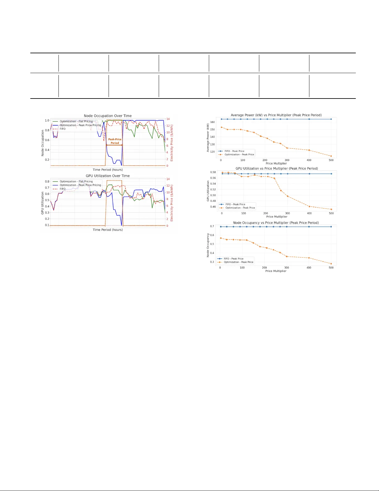
1 A Sensitivity Analysis of Flexibility fr om GPU-Hea vy Data Centers Y iru Ji † , Constance Crozier † , Matthew Liska ‡ Abstract —The rapid growth of GPU-heavy data centers has significantly increased electricity demand and creating challenges for grid stability . Our paper inv estigates the extent to which an energy-awar e job scheduling algorithm can provide flexibility in GPU-heavy data centers. Compared with the traditional first- in first-out (FIFO) baseline, we show that mor e efficient job scheduling not only increases profit, but also brings latent power flexibility during peak price period. This flexibility is achieved by moving lower energy jobs, prefer entially executing jobs with lower GPU utilization and smaller node requir ements, when the electricity price is high. W e demonstrate that data centers with lower queue length and higher variance in job characteristics such as job GPU utilization and job size, offer the greatest flexibility potential. Finally we show that data center flexibility is highly price sensitive, a 7% demand reduction is achieved with a small incentive, but unrealistically high prices are required to achieve a 33% reduction. Index T erms —Data Center , Energy Optimization, Demand Response, Job Scheduling, Grid Flexibility N O M E N C L A T U R E Sets J Set of all jobs S ( j, τ ) Set of start times for job j to be activ e at τ T current Set of time steps in the current time window V ariables p cont j,τ Power of continuing job j at time τ (kW) p new j,τ Power of newly-started job j at time τ (kW) p total τ T otal power consumption at time τ (kW) t end j End time of job j t start j Start time of job j x cont j,τ 1 if job j continues from previous window at time τ x sched j 1 if job j is already scheduled, otherwise 0 x start j,τ 1 if job j starts at time τ , otherwise 0 Parameters c Elec Electricity price at time τ ($/kWh) c GPU Monetary value per GPU-hour ($/GPU-hour) d j Duration of job j (Hour) g j Number of GPUs requested by job j H Length of rolling time window (Hour) N T otal number of av ailable nodes in the data center n j Number of nodes required by job j p GPU Activ e power consumption per GPU (kW) p idle Idle power consumption per node (kW) t arr j Arriv al time of job j t wait Maximum wait time allowed for jobs (Hour) T end End time of the rolling time window T start Start time of the rolling time window u j GPU utilization rate of job j α Cooling coefficient † J. Y i and C. Crozier are with the School of Industrial and Systems Engineering, Georgia Institute of T echnology , Atlanta, GA, USA. Email: yji332@gatech.edu ‡ M. Liska is with the School of Physics, Georgia Institute of T echnology , Atlanta, GA, USA. I . I N T RO D U C T I O N In recent years, data centers hav e emerged as critical in- frastructure components for the digital economy , with their power consumption growing rapidly due to the expansion of artificial intelligence and cloud computing services [1]. Current projections indicate that data centers may consume approximately 10% of the nationwide electricity demand by the end of this decade [2]. This growth brings great challenges for grid operators, who must cope with sudden increases in electricity demand while maintaining the stability and reliability of the system. T o address these challenges, extensiv e research has explored the optimization of job scheduling within data centers to improv e operational efficiency . V arious algorithmic frame- works hav e been proposed, ranging from greedy heuristics [3], mixed-integer linear programming [4], to reinforcement learning that adapt to dynamic operating conditions [5]–[7]. Although traditional approaches primarily emphasized per- formance metrics such as throughput, latency , and resource utilization, recent work has ev olved tow ard energy-aware scheduling strategies that consider electricity costs and carbon emissions. These strate gies incorporate cooling control [5], renew able energy utilization [8], and participation in electricity markets [9], [10], recognizing the complex interplay between computational workloads, energy systems, and external market conditions. These research shows that jobs with varying time sensitivity and resource requirements can create opportunities for flexible scheduling approaches that can intelligently prior- itize and allocate resources [11]. Building on these opportunities, researchers hav e dev eloped various approaches to incenti vize and manage flexibility in data center operations. Sev eral studies have focused on incen- tiv e mechanisms for delay-tolerant workloads using optimiza- tion frameworks [12] as well as game-theoretic approaches [13], to balance operational costs against flexibility re wards while maintaining acceptable service quality . Other research consider contractual framew orks between data center and grid operators [14], leader-follo wer game models [15], and learning-based approaches for dynamic resource management [8], all aimed at leveraging the inherent flexibility in data center operations. Although recent work has begun to explore the potential of data centers to provide grid flexibility [16], limited research has systematically quantified the fle xibility potential of modern GPU-heavy data centers or analyzed the sensiti vity of this fle x- ibility to various operational parameters. Our work addresses these gaps by dev eloping a detailed scheduling framew ork that incorporates realistic workload characteristics and tests its response to different price events. Specifically , we 1) quan- tify the flexibility potential of GPU-heavy data centers with delayable workloads, 2) show that the flexibility is achiev ed 2 by prioritizing low power consumption jobs, characterized by lower GPU po wer utilization and fe wer node requirements, and 3) analyze the sensitivity of this potential to key operational parameters in data centers, such as queue length and job heterogeneity . Our work bridges the gap between theoretical models and real-world implementation challenges. I I . B A S EL I N E D AT A C E N T E R O P E R AT I O N This section introduces the basic components in data center and the scheduling logic that is currently most commonly employed in data center operations. In this paper , we focus on data centers which compute large delayable jobs on GPUs, such as AI training or HPC simulations. A. P arameter definitions A GPU-hea vy data center operates as a complex system, where understanding key operational concepts is essential for optimizing resource allocation and energy efficienc y . When a job cannot fully utilize all the GPUs in the allocated node, resource fragmentation occurs, reducing overallNodes and GPUs represent the fundamental computing architecture in a data center . A node typically refers to a complete physical server , including processors, memory , local storage, and networking components. GPUs are specialized accelera- tors installed within these nodes. A typical high-performance computing node may contain 1 to 8 GPUs, interconnected via high-speed buses. W orkloads usually request resources based on the number of GPUs. efficiency . Node occupation reflects the proportion of av ailable nodes currently running jobs, e xpressed as the ratio of allocated nodes to the total number of nodes. High occupancy indicates efficient use of the physical infrastructure, but may limit the system’ s flexibility in responding to new job scheduling requests. GPU utilization reflects the extent to which GPU power is actually being utilized. Unlike node occupation, which focuses on physical resource allocation, GPU utilization measures how close the GPU is operating to its thermal design power (TDP) limit. For example, computationally intensi ve tasks high in matrix arithmetic and floating point operations can often max out the TDP , leading to high GPU power utilization. In contrast, operations like memory transfers—e ven at peak memory bandwidth—typically consume less power and thus result in lower power utilization. The cooling system is responsible for managing the large amount of heat generated by the computing hardware. As the GPU density and po wer intensity increases, so does the cooling requirements. Modern data centers employ a variety of strategies, but as traditional air cooling methods become inadequate, operators typically switch to liquid cooling and in the future also immersion cooling. B. State-of-the art scheduling The first-in first-out (FIFO) with backfilling algorithm is currently widely used in high-performance computing job scheduling. In basic FIFO, jobs are processed strictly in arri val order , which might lead to resource under-utilized when large jobs block smaller ones. Backfilling addresses this limitation by allowing smaller or lower -priority jobs to use idle resources ahead of time, b ut only if doing so does not delay the expected start of any earlier arri ving jobs. This is achiev ed by calculating a timeline based on the estimated completion times of running jobs. If a gap appears before a high-priority job needs its resources, a qualifying lower-priority job can be scheduled into this gap immediately [17]. I I I . E N E R G Y - A WAR E S C H E D U L I N G A L G O R I T H M In this section, we will introduce our proposed energy-a ware scheduling algorithm. The algorithm proceeds in two main stages: first, we formulate and solve an optimization model to determine optimal job start times within a static time window; second, we describe the rolling-horizon procedure that applies this model sequentially across the entire scheduling horizon to obtain a complete schedule. A. Optimization over a static time window Our optimization model operates under the assumption of perfect knowledge within the time window , where job arriv al times, GPU utilization, node requirements, and durations are known in adv ance. Further , within each static windo w , we also consider that some jobs may already be running from the previous window . This allows us to formulate the following deterministic scheduling problem. For each current time windo w T current , we solve the follo w- ing optimization problem to determine when each of the jobs will be executed: max Z = X j ∈J : x sched j =0 c GPU · g j · d j · X τ ∈T current x start j,τ − X τ ∈T current (1 + α ) · c Elec · p total τ The objectiv e function maximizes profit by considering job rev enue, electricity and cooling costs. The revenue term calcu- lates the total rev enue from scheduling jobs, where x sched j is a binary variable indicating whether job j has been scheduled in a previous time window or not (1 if scheduled, 0 otherwise), c GPU represents the monetary value per GPU-hour , g j denotes the number of GPUs requested by job j , d j is the duration of job j , and x start j,τ is a binary variable indicating whether job j starts at time τ . Therefore, the first term in the objectiv e function represents the profit gained from jobs starting in the current time window T current , and the second term considers the electricity and cooling cost. The total power consumption at time τ is defined as: p total τ = p idle · N + X j ∈J  p cont j,τ + p new j,τ  with: S ( j, τ ) =  s ∈ T current : max( t arr j , τ − d j + 1) ≤ s ≤ τ  p cont j,τ = x cont j,τ · g j · u j · p GPU 3 p new j,τ = g j · u j · p GPU · X s ∈S ( j,τ ) x start j,s The total power consumption p total τ includes a fixed idle power component p idle · N representing the idle energy con- sumption of all av ailable nodes, plus a dynamic component proportional to the number of acti vely utilized GPUs. For each job j and time step τ , the set S ( j, τ ) contains all possible start times s within the current time window that would result in job j being activ e at τ . Specifically , a start time s ensures the job starts no earlier than its arri val time and no later than τ , while also ensuring the job’ s duration would cover the required τ time steps. Therefore, the power of acti ve nodes can be calculated by both jobs continuing from previous time windows p cont j,τ and jobs starting within the current window p new j,τ , where u j is the GPU utilization rate and p GPU is the activ e power consumption per GPU, which is calculated as the difference between maximum node power and idle node power divided by the number of GPU nodes. The electricity cost contains time-varying electricity prices c Elec and includes a cooling coefficient α to account for cooling-related energy expenses. The optimization problem is subject to the following oper- ational constraints: X τ ∈T current x start j,τ ≤ 1 ∀ j ∈ J x sched j =0 (1) x start j,τ = 0 ∀ j ∈ J , ∀ τ ∈ T current : τ < t arr j (2) X τ ∈T current τ · x start j,τ ≤ t arr j + t wait ∀ j ∈ J : x sched j = 0 , t arr j ≤ T end (3) X j ∈J  x cont j,τ + X s ∈S ( j,τ ) x start j,s  · n j ≤ N ∀ τ ∈ T current (4) Constraint (1) ensures that each unscheduled job can start at most once within the current time window , preventing multiple start assignments for the same job . Constraint (2) prevents jobs from starting before their specific arriv al times t arr j . Constraint (3) enforces the maximum wait time requirement, ensuring that each job should start within the maximum waiting time t wait after its arriv al, thus preventing job delays. This constraint only applies to jobs whose arriv al time t arr j is before the end of the current time window T end . The running status of jobs is tracked through the variable x cont j,τ , which indicates whether job j is activ e at time τ , accounting for both jobs continuing from previous windows and jobs starting within the current windo w . Constraint (4) guarantees that the total nodes required by all running jobs, including the continuing ones from the previous time window x cont j,τ and jobs starting in the current time windo w x start j,s , do not e xceed the total a vailable node capacity N , where n j represents the number of nodes required by job j . B. Rolling horizon algorithm The rolling horizon algorithm is designed to solve large- scale job scheduling problems by decomposing the entire time horizon into smaller , manageable windows. This approach both allows us to solve for longer time horizons, and to consider the more realistic case where jobs are arriving in real-time. Let T represent the complete set of all time steps in the scheduling horizon, and H denote the rolling horizon length, which defines the size of each optimization window (e.g., H = 24 time steps). The algorithm proceeds iterativ ely , solving an optimization problem for each time window while updating state information between consecutiv e windo ws. At each iteration k = 0 , 1 , 2 , . . . , ⌊|T | /H ⌋ , the current time window T current = [ T start , T end ] is defined, where T start = k · H and T end = min(( k + 1) · H − 1 , |T | ) . The algorithm maintains state variables including job scheduling status ( x sched j ) and start times ( t start j ). Before solving each window’ s optimization, the algorithm updates the status of continuing jobs that started in previous windows but are still running in the current window . The detailed operation of the algorithm can be described as follows: Algorithm 1 Rolling Horizon Algorithm 1: Initialize x sched j = 0 , t start j = − 1 ∀ j ∈ J 2: for each time window k = 0 , 1 , 2 , . . . , ⌊ ( |T | − 1) /H ⌋ do 3: [ T start , T end ] = [ k · H , min(( k + 1) · H − 1 , |T | )] , T current = { T start , . . . , T end } 4: Update x cont j,τ = 1 if x sched j = 1 and t start j < T start ≤ τ < t start j + d j , else 0 5: Solve single window optimization model to deter - mine x start j,τ for { j ∈ J | x sched j = 0 } 6: for each job j where P τ ∈T current x start j,τ = 1 do 7: Update x sched j = 1 and t start j = τ where x start j,τ = 1 8: end for 9: end for In brief, each iteration of the rolling horizon algorithm performs three tasks: identify which jobs are continuing from previous windo ws, solve the optimization in the current time window to schedule new job starts, and update the job status. I V . S I M U L A T I O N S E T U P A N D F L E X I B I L I T Y C A L C U L AT I O N In this section, we will describe the simulation was set up, the parameters that we chose in our experiments, and the method we used to ev aluate the flexibility . A. Simulation set up Our model simulates a GPU-heavy data center with de- layable loads operating over multiple days with a rolling horizon optimization approach. The simulation process begins with generating a realistic workload of heterogeneous jobs with varying resource requirements, durations, and arriv al times. W e synthesized a workload of 150 jobs with arriv al times distributed across a 5-day time window . The time step granu- larity of our simulation is 1 hour, each rolling horizon window is 24 hours, and the total simulation time length is 120 hours. The data center is equipped with 100 nodes with 4 GPUs per node. The maximum and idle power of each node is 3000W [18] and 900W respectiv ely [19]. The cooling coefficient of the data center is 0.4 [19]. 4 Job characteristics follo w distributions deri ved from analysis of real-world GPU cluster w orkloads. Each job requests a specific number of GPUs, with an estimated duration, GPU uti- lization rate, and generates revenue proportional to its resource consumption. T o model realistic GPU allocation patterns, we implemented an inv erse relationship between the number of GPUs requested and the probability of job occurrence – jobs requesting fe wer GPUs appear more frequently than those demanding larger GPU amounts. Furthermore, we assume that 20% of jobs will terminate early before their estimated completion time. T able I summarizes the ke y parameters used in our simula- tion en vironment. T ABLE I S I MU L A T I O N P AR A M ET E R S Parameter V alue Rolling W indow T otal simulation length 120 hours Rolling horizon window 24 hours T ime step granularity 1 hour Data Center P arameters Number of compute nodes 100 GPUs per node 4 Maximum po wer per node 3000W Idle po wer per node 900W Cooling coef ficient 0.4 Job P arameter s Mean job duration 10 hours Standard de viation of duration 6 hours Maximum job duration 48 hours Maximum wait time 30 hours GPU utilization Mean 0.6 Percentage of early terminating jobs 20% Job pricing $2.30 / GPU-hour All experiments were conducted on a system equipped with an ROG Zephyrus G16 GU603VV laptop using Python 3.8 with Gurobi 11.0.3 as the optimization solver . B. T esting flexibility T o ev aluate the flexibility of the data center , we simulate a sudden peak price scenario, which can occur in modern power grids when demand surges, generation fluctuations, or transmission lines become constrained. Data centers with flexible workload management capabilities could provide real- time demand response services during these events. In our experiment, we introduce a significant peak price in the middle of our simulation time range, where the electricity price triples from the baseline rate of $0.45/kWh to $1.35/kWh for a duration of 1 hour . This substantial but short-liv ed price increase simulates a grid-stress e vent, where we assume we know at the start of the window when the ev ent will occur – similar to day-ahead pricing. W e quantify the system’ s flexibility by measuring the differ- ence between the av erage power usage during the peak price period under the dynamic pricing scenario and the average power usage during the same hour in a flat-price scenario. This difference represents the system’ s ability to temporarily reduce load in response to price signals. W e also examine ho w the ov erall operation of the data center is affected, outside of the peak period. V . R E S U LT S W e compare our scheduling algorithm against the FIFO with backfilling model under both the flat and peaking electricity price signals, using the data center simulation described above. Our analysis focuses on multiple metrics including av erage power consumption, av erage GPU utilization rate, average node occupancy rates, and total rev enue. W e examined both the complete simulation duration (excluding first and last time window to mitigate boundary ef fects) and the peak price period for targeted analysis. A. Overall P erformance Comparison W e compare our optimization method with the baseline FIFO approach in T able II. Across the whole simulation pe- riod, we can observe that both methods achiev e similar lev els of average power usage, GPU utilization, and node occupancy . Our optimization method can increase revenue ov er FIFO due to a more optimal scheduling, but in most cases it will result in a slightly higher average job wait time. This represents an expected trade-off between system responsiveness and power flexibility . During the peak price period, the optimization method will hav e a lo wer power consumption, achiev ed by decreasing the overall node occupancy when the electricity price is high. Therefore, our scheduling algorithm provides flexibility without compromising the system’ s overall performance and rev enue across the entire scheduling horizon. T ABLE II P E RF O R M AN C E C O M P A R I SO N B E TW E E N T H E W H OL E P E R I OD A N D P E A K P R IC E P E RI O D All Period Peak Price Period Opt. FIFO Opt. FIFO A verage Power (kW) 176 175 153 164 GPU Utilization 0.55 0.55 0.52 0.51 Node Occupancy 0.74 0.74 0.56 0.69 A verage W ait (h) 1.95 1.67 - - Rev enue (k$) 49.87 49.32 0.51 0.64 B. P eak Price P eriod Analysis Our analysis demonstrates that the data center’ s po wer flexibility during peak pricing periods stems from adjustments in two key dimensions: GPU utilization and node occupancy . During peak price periods, the scheduling algorithm prior- itizes jobs with lower GPU utilization and fav ors scheduling workloads that require fewer nodes. Figure 1 shows ho w the node occupation and GPU utilization rate change over time comparing among the three algorithms: FIFO considering backfilling, our optimized scheduling algorithm with a flat price, and our optimized scheduling with a 10-hour 300 peak price multiplier in the middle of the time window . As illustrated, this leads to a reduction in both the total GPU utilization and the number of occupied nodes, thus reducing power consumption when electricity price are highest. De- creases in GPU utilization show that flexibility is gained by mov ed lower energy jobs into the peak period, while changes 5 T ABLE III C O MPA R IS O N D U R I NG P E AK P R I CE P E RI O D W I T H V A R IE D : G P U U T I L IZ ATI O N V A R I AN C E , N U M BE R O F J O BS , A N D G P U S / J O B R E S P EC T I VE LY . Util=0.6 Util ∼ N(0.6,0.3) Jobs=100 Jobs=200 GPUs/job=20 GPUs/job ∼ P(20) FIFO Opt FIFO Opt FIFO Opt FIFO Opt FIFO Opt FIFO Opt Peak Price 3 300 3 300 3 300 3 300 3 300 3 300 Power (kW) 169 156 138 164 153 125 151 121 109 199 189 138 182 147 124 169 135 119 GPU Util 0.55 0.55 0.55 0.51 0.52 0.42 0.62 0.57 0.52 0.59 0.57 0.45 0.65 0.66 0.65 0.57 0.58 0.49 Occupancy 0.69 0.57 0.41 0.69 0.57 0.36 0.49 0.27 0.17 0.88 0.82 0.49 0.67 0.43 0.28 0.67 0.39 0.28 Rev enue ($) 646 516 363 646 516 311 511 223 144 805 749 433 660 398 255 641 335 258 Fig. 1. Node Occupation and GPU Utilization change ov er time considering peak price with a 300x multiplier . in utilization show that gaps in the scheduling (typically some are unav oidable) are rearranged into the period. Furthermore, Figure 2 compares FIFO algorithm consid- ering backfilling and optimization model, and shows how the av erage power , GPU utilization and node occupancy rate during the peak price period change under different peak price multiplier , ranging from 3 to 500, under the two cases. It rev eals that this flexibility response is highly price-insensitiv e within a realistic operating range. W e see that some flexibility occurs at an extremely small price spike, mainly caused by the reduction in node occupancy . A significant response only occurs under extreme price multipliers (exceeding 100); at this point, the system aggressiv ely reduces both GPU utilization and node occupancy to mitigate costs. C. Sensitive Analysis on differ ent job characteristics It is likely that our results are influenced by out chosen job parameters, and thus that some data centers will exhibit more flexibility than others. Through table III, we analyze the impact of three key job factors: GPU utilization variance, job queue length, and the number of GPUs requested per job, to identify the factors that determine a data center’ s potential to provide power flexibility . 1) GPU utilization variance: In T able III we compare the case where all jobs ha ve the same utilization (0.6) to the case where GPU utilization follows a normal distribution with Fig. 2. A verage power usage during peak price period time under different price multipliers. the same mean. This shows that heterogeneity in job GPU utilization is a ke y driv er for flexibility . A workload composed of jobs with di verse GPU utilization le vels allo ws the scheduler to selectively execute low-utilization jobs during peak price periods, thereby reducing power intensity without interrupting service. Whereas, if all jobs ha ve the same utilization then flexibility can only be created from having the nodes idle during the peak period, which we do not see ev en with the 300x price multiplier . As shown in Figure 3, for moderate price increases, such as a price multiplier between 3 and 30, changes in GPU utiliza- tion variance have minimal impact on po wer consumption pat- terns. Howe ver , when the peak price multiplier reaches 300, a workload with high GPU utilization variance enables a 23.8% reduction in power consumption, significantly outperforming the 18.3% reduction achiev ed under a homogeneous utilization profile. This demonstrates that in extreme peak price scenarios, systems with higher GPU utilization v ariance of fer greater opportunities for power optimization. 2) Job Queue Length: W e also test the effect of job queue length, comparing when there are 100 or 200 jobs total (instead 6 Fig. 3. Percentage change of average power during the peak price period compare with FIFO under different peak price and GPU variance. of 150 which is used in the other cases). When the job queue length is shorter , the system can provide more fle xibility . When total job number is 100, which means our queue is short and the data center is not fully occupied, our method reduces po wer consumption by 19.6% compared to FIFO. While when the total job number is 200 and the data center is highly occupied, the room for flexibility is reduced and the po wer reduction is only 4.9%. The less heavily used a data center is, the more latent flexibility can be provided. 3) Number of GPUs per job: The heterogeneity in job size, measured by the number of GPUs requested per job, shows no significant or consistent impact on flexibility potential during peak price period. Under a 3× price multiplier , the optimization achieves a power reduction of 19.2% for fixed- size jobs (20 GPUs each) and 20.1% for variable-size jobs (Poisson-distributed with mean 20). Under an extreme 300× multiplier , the reductions are 31.9% and 29.6%, respectiv ely . This indicates that job-size div ersity is a less significant driver of flexibility compared to the others we study in the analysis. The algorithm can effecti vely shift or defer jobs reg ardless of their GPU count, provided there is sufficient slack in the queue. Thus, while job-size variability may slightly alter the mix of jobs that run during the peak period, it does not substantially enhance the data center’ s flexibility . V I . C O N C L U S I O N In this paper we demonstrate that energy-aware scheduling enhances both the economic performance and grid flexibility of GPU-heavy data centers. W e show that, compared to tra- ditional scheduling (first-in first-out with backfilling), energy- aware scheduling consistently increases ov erall profit through a more intelligent job allocation without compromising job throughput. More importantly , we quantify the latent flexibility potential in data centers, showing that power consumption can be re- duced during the peak price period. This is achie ved primarily through aligning unav oidable gaps in node occupancy with the peak period, and at higher prices by aligning lo wer energy jobs with the peak period. Some degree of flexibility exists at low prices, which increases substantially as the maximum price multiplier increases. Through sensitivity analysis, we identify two key character- istics that maximize flexibility potential: (1) data centers with lower queue utilization, which provides greater scheduling freedom, and (2) workloads with higher variance in job characteristics, particularly GPU utilization rates. This het- erogeneity enables the scheduler to prioritize energy-ef ficient jobs during high-price periods without compromising ov erall service quality . R E F E R E N C E S [1] A. Shehabi, A. Newkirk, S. Smith, A. Hubbard, N. Lei, M. Siddik, et al. , “2024 United States Data Center Energy Usage Report, ” T ech. Rep. LBNL-2001637, Lawrence Berkeley National Laboratory , 2024. [2] T . Norris, T . Profeta, D. Patino-Eche verri, and A. Cowie-Haskell, “Rethinking load growth: Assessing the potential for integration of large flexible loads in us power systems, ” 02 2025. Retriev ed from https://hdl.handle.net/10161/32077. [3] Z. Dong, N. Liu, and R. Rojas-Cessa, “Greedy scheduling of tasks with time constraints for energy-ef ficient cloud-computing data centers, ” Journal of Cloud Computing , vol. 4, no. 1, p. 5, 2015. [4] H. Guo, H. Y u, M. W ang, C. Liu, and C. Li, “Integrated management of workloads and energy system for data centers, ” Energy , p. 136400, 2025. [5] K. Shi, S. Chen, S. Chen, Y . Sun, and Z. Ding, “Ener gy-aware data center job scheduling scheme under uncertain en vironment, ” in 2024 IEEE/IAS 60th Industrial and Commercial P ower Systems T echnical Conference (I&CPS) , pp. 1–6, IEEE, 2024. [6] Y . Ran, H. Hu, X. Zhou, and Y . W en, “Deepee: Joint optimization of job scheduling and cooling control for data center energy efficiency using deep reinforcement learning, ” in 2019 IEEE 39th International Confer ence on Distributed Computing Systems (ICDCS) , pp. 645–655, IEEE, 2019. [7] W . Liu, Y . Y an, Y . Sun, H. Mao, M. Cheng, P . W ang, and Z. Ding, “Online job scheduling scheme for low-carbon data center operation: An information and ener gy nexus perspectiv e, ” Applied Ener gy , vol. 338, p. 120918, 2023. [8] C. Xu, K. W ang, P . Li, R. Xia, S. Guo, and M. Guo, “Renewable energy-a ware big data analytics in geo-distributed data centers with reinforcement learning, ” IEEE T ransactions on Network Science and Engineering , v ol. 7, no. 1, pp. 205–215, 2018. [9] H. Y uan, H. Liu, J. Bi, and M. Zhou, “Revenue and energy cost- optimized biobjective task scheduling for green cloud data centers, ” IEEE T ransactions on Automation Science and Engineering , vol. 18, no. 2, pp. 817–830, 2020. [10] K. Lee and Y . Kim, “Online pricing and resource scheduling for profit maximization of cloud storage providers, ” IEEE T ransactions on Cloud Computing , 2024. [11] W . Y ang, H. Qv , X. W ei, and Z. Ding, “Pricing temporal flexibility of data center jobs with heterogeneous time constraints, ” in 2025 IEEE Industry Applications Society Annual Meeting (IAS) , pp. 1–6, IEEE, 2025. [12] D. Paul, W .-D. Zhong, and S. K. Bose, “Demand response in data centers through energy-ef ficient scheduling and simple incentivization, ” IEEE Systems J ournal , vol. 11, no. 2, pp. 613–624, 2015. [13] Y . Guo, H. Li, and M. Pan, “Colocation data center demand response using nash bargaining theory , ” IEEE T ransactions on Smart Grid , vol. 9, no. 5, pp. 4017–4026, 2017. [14] R. Basmadjian, J. F . Botero, G. Giuliani, X. Hesselbach, S. Klingert, and H. De Meer, “Making data centers fit for demand response: Introducing greensda and greensla contracts, ” IEEE transactions on smart grid , vol. 9, no. 4, pp. 3453–3464, 2016. [15] O. Han, T . Ding, C. Mu, W . Jia, Z. Ma, and F . Li, “ A two-stage demand response stackelberg game of data center operators and the system operator based on kriging metamodel, ” IEEE Tr ansactions on Automation Science and Engineering , vol. 21, no. 4, pp. 6666–6679, 2023. [16] C. Crozier and M. Liska, “The potential of data center energy demand to provide grid fle xibility , ” Curr ent Sustainable/Renewable Ener gy Reports , vol. 12, no. 1, pp. 1–6, 2025. 7 [17] M. A. Jette and T . Wickber g, “ Architecture of the slurm workload man- ager , ” in W orkshop on Job Scheduling Strate gies for P arallel Processing , pp. 3–23, Springer, 2023. [18] NVIDIA Corporation, “NVIDIA H200 T ensor Core GPU Datasheet, ” tech. rep., NVIDIA Corporation, 2024. Accessed: January 2026. [19] A. Shehabi, A. Newkirk, S. J. Smith, A. Hubbard, N. Lei, M. A. B. Siddik, B. Holecek, J. Koome y , E. Masanet, and D. Sartor , “2024 united states data center energy usage report, ” 2024.