Tracking without Seeing: Geospatial Inference using Encrypted Traffic from Distributed Nodes

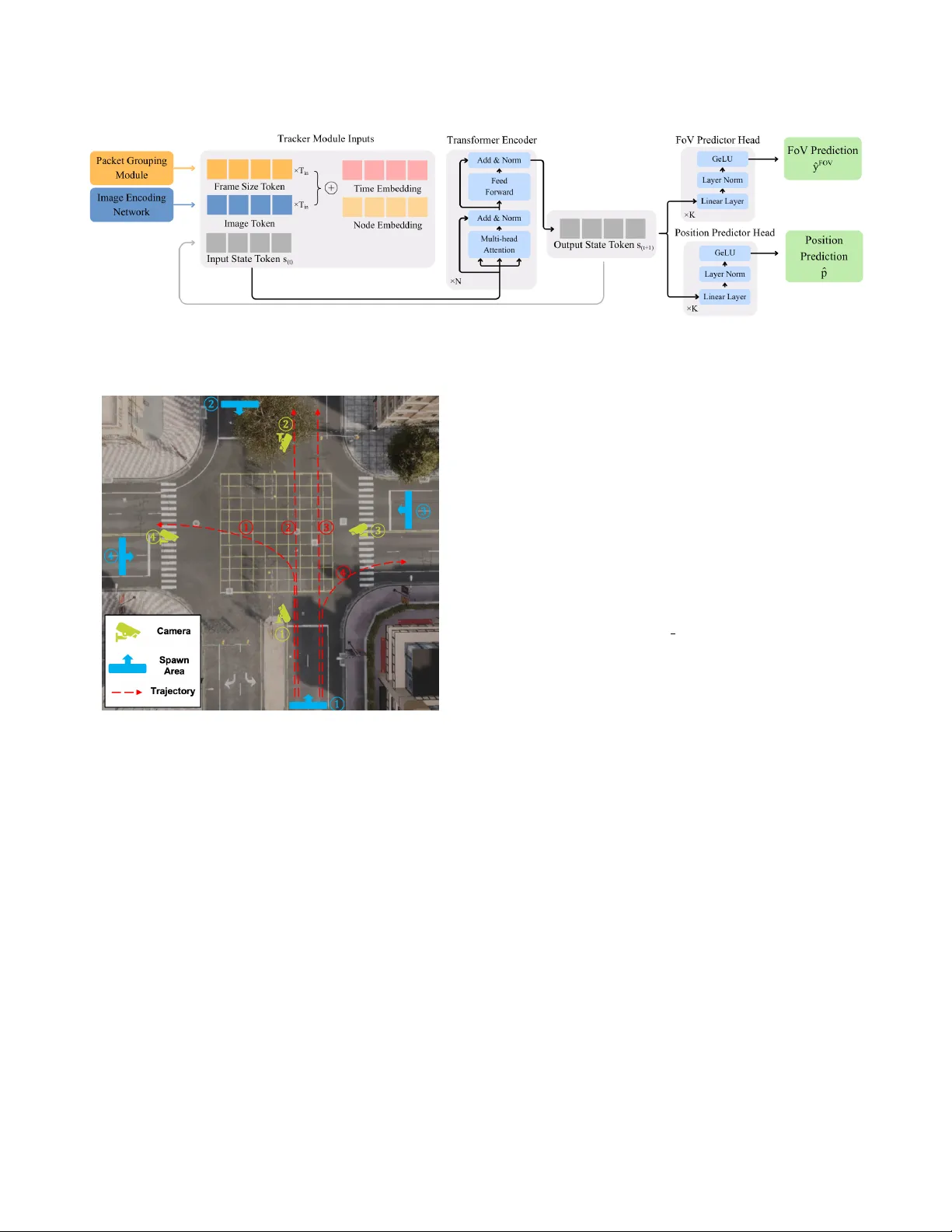
T racking without Seeing: Geospatial Inference using Encr ypted T raic from Distributed Nodes Sadik Y agiz Y etim 1 ∗ , Gaofeng Dong 1 ∗ , Isaac-Neil Zanoria 1 ∗ , Ronit Barman 1 , Maggie Wigness 2 , T arek Abdelzaher 3 , Mani Srivastava 1 , Suhas Diggavi 1 {yagizyetim, gfdong, zanoria, r onitbarman}@ucla.edu, maggie.b.wigness.civ@army .mil, zaher@illinois.edu, {mbs, suhas}@ucla.edu 1 University of California, Los Angeles 2 DEV COM Army Research Laboratory 3 University of Illinois at Urbana-Champaign Abstract Accurate observation of dynamic environments traditionally relies on synthesizing raw , signal-level information from multiple dis- tributed sensors. This work inv estigates an alternative approach: performing geospatial inference using only encr ypted packet-level information, without access to the raw sensory data itself. W e fur- ther explore how this indir ect information can be fuse d with directly available sensory data to extend ov erall inference capabilities. In this paper , we introduce GraySense, a learning-based frame work that performs geospatial object tracking by analyzing indirect infor- mation from cameras with inaccessible streams. This information consists of encrypted wireless video transmission trac, such as network-level packet sizes. GraySense lev erages the inherent rela- tionship between scene dynamics and the transmitted packet sizes of the video str eams to infer object motion. The framew ork consists of two stages: (1) a Packet Grouping module that identies frame boundaries and estimates frame sizes fr om encr ypted network traf- c, and (2) a T racker module, based on a T ransformer encoder with a recurrent state, which fuses these indirect, packet-based inputs with optional direct, camera-based, sensory inputs to estimate the object’s position. Extensive experiments, conducted with realistic videos from the CARLA simulator and emulated networks under varying, imperfect conditions, sho w that GraySense achieves a high tracking accuracy of 2 . 33 meters error (Euclidean distance) without raw signal access. This error is r easonable relative to the smallest tracked object’s dimensions ( 4 . 61 m × 1 . 93 m ), enabling meaningful trajectory estimation. In summar y , we demonstrate a method that performs geospatial inference using only encrypted trac, without access to raw signals. T o the best of our knowledge, such capability has not been previously observed, and it expands the use of latent signals available for sensing. 1 Introduction A comprehensive understanding of dynamic environments increas- ingly depends on integrating information from multiple distributed sensors, whose complementary viewpoints and spatial coverage to- gether pr ovide richer and more r esilient perception of the scene [ 1 – 3 ]. However , in practice, direct access to raw sensor data can be lim- ited. Ownership b oundaries, privacy policies, and encryption pro- tocols restrict systems to operate with only a subset of all available sensors [ 4 , 5 ]. Meanwhile, many nearby sensors remain physically co-located yet logically isolated, broadcasting encrypted network trac that indirectly reects their sensing activity [ 6 – 8 ]. These inaccessible nodes form a latent layer of the environment’s p er- ceptual network - one that cannot be directly obser ved, yet whose ∗ Equal contribution. Figure 1: Application scenario of GraySense. The scene il- lustrates a distributed sensing environment consisting of accessible cameras (blue nodes) and inaccessible cameras (gray nodes) whose video streams are encrypted. While blue nodes provide direct visual input, gray nodes contribute only encrypted network trac, which indirectly reects scene dynamics through variations in packet sizes. transmission dynamics encode meaningful information about the underlying scene. Unlocking this information could extend oppor- tunistic perception, where a system obser ves a scene not just by “seeing” directly , but by listening to the data ows of surrounding sensors. In this work, we use the term “seeing” to refer broadly to having access to raw , signal-level sensory measurements. Thus, “tracking without seeing” denotes the capability to perform geospa- tial inference without access to raw sensor signal. This asymmetry between accessible and inaccessible sensors mo- tivates our exploration of "indirect" sensing. W e categorize sensors into two classes based on their accessibility: blue nodes , which denote sensors directly accessible to the system ( e.g., cameras with available video streams), and gray nodes , which repr esent indirect sensors whose measurements cannot be accessed but encr ypted transmission trac can be passively observed. In this paper , we exclusively use cameras as sensors , as illus- trated in Figure 1. While blue nodes provide conventional visual information, gray nodes contribute only network-level information such as packet sizes. Despite this constraint, the temporal patterns of gray node trac can still provide rich information regarding the innovations in the underlying scene depending on the transmission protocol. Popular video codecs, such as H.264 [ 9 ], primarily encode the dierences between consecutive frames. This process results in signicant frame-size variations that are preserved even after encryption, causing the observed trac to inherently carr y struc- tured information on scene dynamics, which we exploit through a learning-based framework to do geospatial inference. 1 Recent studies have shown that encrypted vide o streams can pro- vide information on the dynamics of the monitored environment. For instance, Li et al. [ 10 ] demonstrated that side-channel informa- tion in encrypte d surveillance video trac can be exploited to infer coarse activity patterns such as the presence or movement of p eople within a scene. Similarly , Huang et al. [ 6 ] highlighted privacy risks from wireless surveillance cameras by showing that encrypted traf- c features can re veal basic human activities. Mari et al. [ 8 ] went beyond activity detection to infer r ough walking directions from encrypted video-surveillance trac. Rasool et al. [ 7 ] further de- veloped non-machine-learning methods for detecting motion and person presence. How ever , these approaches do not analyze ho w frame-level dynamics relate to the underlying scene geometry , and typically rely on trac from a single gray no de. Furthermore, they treat the problem as a classication or detection task without ex- plicitly modeling or reconstructing any spatial information fr om the scene. Building on these prior work on single-object sensing, GraySense prioritizes single-target tracking to match monitoring requirements in high-stakes se curity perimeters, where a single intruder constitutes a critical state transition and maintaining ro- bust position estimation is the primar y objective. This aligns with single-threat validation protocols used in sterile-zone surveillance [ 11 , 12 ]. A similar framing appears in search and rescue, where the goal is often to locate a specic target [ 13 ]. Extending GraySense to the multi-object setting is discussed in Section 8. In this work, we systematically investigate the relationship be- tween scene dynamics and encr ypted trac patterns, and propose the GraySense framework for geospatial object tracking using en- crypted WiFi camera trac. By leveraging multiple distributed sensors, blue nodes and gray nodes, we demonstrate that it is possible not only to detect motion but to continuously track an object’s position from the encrypted network trac , re- vealing a previously unexplored capability , =which oers several compelling advantages. By relying solely on packet-size informa- tion in video transmissions, GraySense enables object tracking without access to raw camera streams , providing an alternative to conventional vision-based tracking. Moreover , when combined with available blue nodes, information from surrounding gray nodes can extend the eective sensing range and maintain target conti- nuity even after the object leaves the eld of view of accessible cameras. Finally , since it operates on lightweight network metadata rather than raw image or video data, GraySense brings signicant reductions in computational and communication complexity , mak- ing it well-suited for scalable deployment across distributed or resource-constrained sensing systems. Although promising, GraySense faces se veral challenges. First, extracting useful frame-level information, such as frame b ound- aries and relative frame sizes, from encr ypted network trac is nontrivial, especially under network imperfections such as band- width limit, variable delay , and jitter . These ee cts obscure temporal 1 W e b elieve the ov erall idea of using structure in packets induce d by compression can be applied to other formats as well, which are discussed in Section 3.1. regularities and make frame segmentation unreliable. Second, while packet-level trac from a single gray node encodes aggregate tem- poral patterns that correlate with scene dynamics, it conveys only a total measure of change , without any explicit spatial context of where this change occurs. In other wor ds, packet sizes provide a compressed, viewpoint-specic signal that integrates motion over the entire eld of view , making spatial localization highly challeng- ing. This limitation introduces signicant ambiguity , as multiple scene congurations can produce similar packet-size sequences. Third, the absence of existing datasets that couple ground-truth trajectories, video content, and realistic network traces hinders the development and evaluation of learning-based approaches. T o address these challenges, we intr oduce GraySense with fol- lowing advances. First, we de velop a Packet Grouping module used for inferring frame boundaries from raw encr ypted packet streams, reconstructing frame-le vel structure even under noisy net- work conditions. Second, we develop a Tracker mo dule built on a Transformer encoder [ 14 ] with a recurrent state, which fuses information fr om multiple distributed gray no des and optional blue nodes. By leveraging complementary viewpoints across these sen- sors, the module jointly learns from multi-vie w encr ypted streams to recover spatial structure from non-spatial measurements, en- abling accurate trajectory estimation. Third, to enable systematic training and validation, we construct a suite of realistic synthetic datasets using the CARLA simulator coupled with controlled network emulation , capturing diverse trac conditions, trajecto- ries, and environmental variations. Extensive experiments demonstrate that GraySense achieves 2 . 33 m tracking error using only the encrypted trac from four gray nodes, under noisy network conditions. These results demonstrate that accurate object tracking is achievable using only encr ypted network trac, without accessing any sensor dir ectly . This work validates the concept of tracking without se eing through Gray- Sense , which extends the sensing capabilities of blue nodes by leveraging gray nodes and opens new avenues for future r esearch. Our key contributions are summarized as follows: • W e develop a novel framew ork for geospatial obje ct tracking us- ing encrypted trac fr om gray nodes and optional video str eams from blue nodes within distributed sensing systems, and demon- strate its underlying feasibility through geometric analysis. • W e pr opose a two-stage learning framework that performs track- ing by combining a Packet Grouping module with a Transformer- based Tracker network, designing a customized loss function and a recurrent-state design to enable consistent tracking. • W e construct a comprehensive suite of realistic synthetic datasets covering diverse scenarios and network conditions, which will be publicly released upon acceptance to foster future research 2 . Extensive experiments validate the eectiveness of GraySense, demonstrating accurate and robust tracking performance under a wide range of sensing and network congurations. 2 Related W ork This work connects to several r esearch directions, including wire- less side-channel analysis, human activity inference from WiFi 2 https://github.com/nesl/graysense 2 trac, and signal-based camera eavesdropping. W e briey discuss their relevance and contrast them with our approach. 2.1 Locating Hidden Cameras via WiFi Trac Recent eorts have lev eraged wireless side channels to detect or lo- calize hidden cameras through analysis of their WiFi transmissions. Systems such as SnoopDog [ 15 ], Lumos [ 16 ], and LocCams [ 17 ] identify the presence and position of surveillance devices by in- troducing controlled environmental motion and correlating the re- sulting trac patterns with known motions. In contrast, our work assumes that camera parameters are already known and fo cuses on the inverse problem - inferring object motion and trajectory from encrypted trac emitted by known cameras. Rather than detecting cameras, we use them as sources of motion-related in- formation, turning their encrypted transmissions into an indirect sensing modality . 2.2 Inferring Human Motion from WiFi Trac A parallel line of research explores using WiFi trac itself to infer human activities or coarse spatial regions in smart-home or indo or settings. Li et al. [ 10 ] and Huang et al. [ 6 ] demonstrated that en- crypted video streams leak information correlated with physical motion, enabling detection of human activities. Rasool et al. [ 7 ] proposed a non-machine-learning method for live-streaming and motion detection through encrypte d trac analysis, while Mari et al. [ 8 ] further inferred walking directions from video-surveillance data. These studies reveal that encrypted network trac contains latent motion cues but are limited to classication or detection tasks. In contrast, our framework performs continuous geospatial tracking, reconstructing object trajectories rather than categoriz- ing activities, and extends the analysis to multi-node, distributed settings with both accessible ( blue) and inaccessible (gray ) sensors. 2.3 Tracking with Compressed Domain Information Prior studies have explored object detection and tracking using information from the compressed video domain rather than raw pixels. MVmed [ 18 ] combines a standard pixel-domain detector (e.g., Faster R-CNN) that runs intermittently on I-frames with a high-speed compressed-domain tracker , predicting object locations between full detections by averaging motion vectors within the last known bounding box. A complementary line of work, Moustafa et al. [ 19 ] directly feed sparse residual frames into a neural network, showing that residuals alone can serve as lightweight and privacy- preserving tracking features, though they still require access to decoded motion information rather than encrypte d data. More r e- cently , Tian et al. [ 20 ] proposed a secure deep learning framework for moving object detection in compressed video using Encrypted Domain Motion Information (EDMI). Their method op erates with- out full de cryption or decompression by designing three motion feature maps derived fr om intentionally unencrypted coding fea- tures such as partition patterns and the number of coding bits at the block level. These features pro vide a coarse spatial representation of motion, revealing which 16 × 16 blocks are complex or frequently subdivided, thus enabling low-resolution motion inference while preserving partial encr yption. In contrast, our framework does not Figure 2: Group of Pictures (GOP) in H.264. Each group starts with an I-frame which is encoded independently . P and B frames are encoded based on their dierence from the ref- erence I or P frames. Due to this dierential encoding, the packet-size variations are informative regarding the total change in the scene. assume any selectively unencr ypted features or access to codec internals, instead inferring scene dynamics solely from encrypted packet-level trac. 2.4 Recovering Images from Electromagnetic Side Channels Orthogonal to network-based approaches, EM Eye [ 21 ] demon- strates that electromagnetic (EM) emissions from embedded cam- eras can be exploited to reconstruct images of the observed scene. While impressive in delity , this method requires close proximity (typically within meter lev el) and dense sensor placement due to the rapid signal attenuation of EM leakage. Our appr oach instead operates over standard wireless network channels, oering a longer eective range. GraySense aims to r ecover motion-level informa- tion rather than pixel-level imagery , providing a scalable alternative to physical side-channel imaging. 2.5 Tracking with Non-visual Modalities A rich body of research has investigated non-visual modalities to augment visual sensing and tracking, such as acoustic [ 22 , 23 ], T oF [ 24 ], and radar systems [ 25 , 26 ]. Distinct from these eorts, GraySense enables inference even without access to raw signals, using only encrypted trac from gray nodes. 3 Background and Problem Formulation 3.1 Background W e focus on videos encoded using the H.264/MPEG-4 codec, one of the most widely used video compression standar ds [ 9 ]. H.264 en- ables ecient transmission by partitioning the stream into a Group of Pictures (GOP) , a set of consecutive frames encoded jointly . A visual description of GOP structure is given in Figure 2. T ypi- cally , the rst frame in each GOP , the I-frame (Intra-code d) , is encoded indep endently , while the remaining frames are encoded dif- ferentially to reduce temporal redundancy . P-frames (Predictive) are encoded using motion-compensate d prediction from preceding reference frames (I- or P-frames). B-frames (bidirectional frames) exploit both past and future reference frames for compression, but this bidirectional dependency inherently requires re-ordering and buering, thereby increasing end-to-end latency . For latency- sensitive applications such as live video surveillance, many systems therefore disable or minimize the usage of B-frames in order to reduce delay [ 10 ]. In this work, we utilize a conguration of I and P-frames without B-frames. Because of this dierential coding 3 structure, the encrypted packet sizes convey information about the innovation, the change in the scene between consecutive frames. 4 Problem Formulation W e let 𝑡 denote the frame index and 𝑇 the total numb er of frames in an experiment. The position of the object at frame 𝑡 is represented by the vector p 𝑡 . W e dene an object as visible at frame 𝑡 if it is in the Field of View (Fo V) of at least one sensor in the network. The sensor network consists of 𝑁 𝐵 Blue Nodes and 𝑁 𝐺 Gray Nodes . • Blue Nodes: Cameras with accessible raw signal-level video streams. The input from the 𝑘 -th Blue Node is de- noted as X ( 𝐵 ) 𝑘 , representing a sequence of v ectors of length 𝑇 . • Gray Nodes: Cameras where only snied packet-level bit- rates are accessible. The input from the 𝑘 -th Gray Node is X ( 𝐺 ) 𝑘 , which is also a sequence of length 𝑇 . Our obje ctive is to perform inference on the observed scene, specically tracking a vehicle’s trajectory , using the set of packet size sequences { X ( 𝐺 ) 𝑘 } 𝑁 𝐺 𝑘 = 1 , with or without the raw video data { X ( 𝐵 ) 𝑘 } 𝑁 𝐵 𝑘 = 1 . 4.1 System Assumptions and Constraints T o ensure the tractability of the tracking problem and the con- sistency of the learne d features, GraySense operates under the following assumptions: (1) Single Obje ct and Background: W e assume a single- object constraint, where at most one target resides within the Fo V of sensors at any time. Furthermore, the back- ground is assumed to be largely static. (2) Codec and GoP Settings: The video encoding parameters, specically Group of Pictures (GoP) structure , are xed. (3) Sensor Conguration: The sensor network has a xed conguration of identical nodes. W e assume b oth the in- trinsic parameters and the poses of each node remain xed between training and inference. The practical implications of these assumptions are further an- alyzed in Section 8, where we also outline potential strategies to relax these constraints and extend the framew ork’s versatility to more complex, dynamic environments. 5 Solution Overview GraySense is a learning-base d framework that estimates an object’s trajectory by processing encrypte d packet-size information fr om the gray nodes. It can also fuse this indirect information with data from accessible camera streams, blue nodes, when available. As shown in Figure 3, the framework’s rst stage, the Packet Grouping mo dule, processes the raw stream of encrypte d WiFi packets. Its primary function is to extract a structured time series of estimated frame sizes from the snied packets. This is a non-trivial task, as the observed packet information is often noisy due to net- work factors like bandwidth limitations or delay , limiting the ee c- tiveness of inexible time-windowing-based approaches [ 8 , 10 ] to packet trace segmentation. T o overcome this, we use a transformer encoder-based model that learns to distinguish the boundaries of transmitted frames under network noise, allowing for accurate frame size reconstruction. Additionally , if a blue node is available, the raw images are processed by a Convolutional Neural Network (CNN) to extract useful visual features. The grouped packet-size time series and optional image features are then passe d to the Tracker module. Using a Transformer En- coder with a recurrent state to maintain consistency for tracking, Tracker processes windows of the input data to perform two sequen- tial tasks. It performs binar y classication for vehicle’s presence in the scene, followed by a position estimation if a vehicle is detecte d. For clarity , we dene several terms used throughout this work. The packet size refers to the raw size (in bytes) of each encrypted network packet captured from a video transmission stream - these are the inputs to the Packet Grouping module. The grouped packet size or extracted/estimated frame size denotes the total size of all packets corresponding to an enco ded video frame, estimate d by the Packet Grouping module. For comparison, the (raw) frame size refers to the ground-truth frame-size information obtained directly from the original enco ded video, prior to transmission over the network. W e use extracted frame sizes generated by the Packet Grouping mo dule as inputs to the Tracker mo dule unless stated otherwise. 6 Solution Details This section provides the details of our solution approach. W e begin with a geometry-based analysis that explains how raw frame size information enables object tracking. W e then verify this approach experimentally in a controlled environment, using the results to build intuition and oer a p ossible explanation for the inner dynam- ics of our learning-based method. Finally , we describe the neural network architectures and loss functions for the packet size extrac- tion and tracking stages in GraySense. 6.1 Geometric Solution: From Frame Sizes to Position via Projection Area While H.264 frame sizes only provide an aggregate, non-spatial measure of the change in the scene, GraySense recovers spatial information by fusing frame size information from distinct views. This works because when the background is static, the change in the scene, hence the frame size, is dominated by object motion, and its magnitude is correlated with the object’s projected area. This area is a function of the object’s p osition, which allows GraySense to fuse measurements fr om non-degenerate views to localize the object. W e hypothesize that the tracker module implicitly estimates this area for each gray no de from the frame-size stream and, by fusing area estimates across distinct camera views, reconstructs the object’s position. W e validate this hypothesis in a controlled environment using the Genesis simulator [ 27 ]. The setup is shown in Figure 4. T o formalize the ge ometric problem, we dene the sphere ’s cen- ter in world coordinates at time 𝑡 as p 𝑡 = [ 𝑥 𝑡 , 𝑦 𝑡 , 𝑧 ] ⊤ , where 𝑧 is known and xed. For camera 𝑖 with extrinsic parameters (rota- tion matrix R 𝑖 and center c 𝑖 ), the sphere’s center in the camera’s coordinate system, p i 𝑡 , is inferred by the transformation [28]: 4 Figure 3: System overview of GraySense. Information on frame sizes extracted by Packet Grouping along with the extracted image information is fe d to the Tracker module which estimates obje ct’s visibility by the sensors and its position when it is visible. Figure 4: The Genesis setup used for geometric analysis. Four identical cameras are looking towards the sphere. The blue polygon shows the area in which the sphere moves, a region always visible to all cameras. In each experiment, the sphere moves at a random but constant velocity b etween randomly sampled initial and nal points within this area. p i 𝑡 = R ⊤ 𝑖 ( p 𝑡 − c 𝑖 ) (1) T o nd the projected area, we rst need to mathematically de- scribe the sphere ’s silhouette on camera’s image plane. A p oint ( 𝑢, 𝑣 ) on the image plane ( 𝑧 = 𝑓 𝑖 ) is part of the silhouette if the ray , m , originating from the camera center (origin) and passing through the point [ 𝑢 , 𝑣 , 𝑓 𝑖 ] ⊤ is tangent to the sphere . This is visualized in Figure 5. The tangency condition requires the distance from the sphere ’s center p i 𝑡 = [ 𝑥 𝑖 𝑡 , 𝑦 𝑖 𝑡 , 𝑧 𝑖 𝑡 ] ⊤ to the ray m to be equal to the sphere ’s radius 𝑟 . Using the cross-pr oduct formula for the distance from a point to a line [29], we get the following: 𝑟 = ∥ p i t × 𝛼 m ∥ 2 ∥ 𝛼 m ∥ 2 = ∥ p i t × [ 𝑢, 𝑣 , 𝑓 𝑖 ] ⊤ ∥ 2 ∥ [ 𝑢, 𝑣 , 𝑓 𝑖 ] ⊤ ∥ 2 . (2) Figure 5: Ge ometric problem. The bold lines denote rays ema- nating from the camera center . Those rays that are tangent to the sphere interse ct the image plane along an ellipse, form- ing the sphere ’s silhouette in the image plane. Simplifying Eq. (2) gives the quadratic equation for the silhouette (where 𝑥 𝑖 , 𝑦 𝑖 , 𝑧 𝑖 are the coordinates of p i 𝑡 ): ( 𝑥 𝑖 𝑢 + 𝑦 𝑖 𝑣 + 𝑧 𝑖 𝑓 𝑖 ) 2 − ( 𝑢 2 + 𝑣 2 + 𝑓 2 𝑖 ) ( 𝑥 2 𝑖 + 𝑦 2 𝑖 + 𝑧 2 𝑖 − 𝑟 2 ) = 0 (3) This equation describes an ellipse on the image plane with the center: ( 𝑢 𝑜 , 𝑣 𝑜 ) =  𝑧 𝑖 𝑓 𝑖 𝑧 2 𝑖 − 𝑟 2 𝑥 𝑖 , 𝑧 𝑖 𝑓 𝑖 𝑧 2 𝑖 − 𝑟 2 𝑦 𝑖  (4) For a centered ellipse in the form 𝐴 𝑢 2 + 𝐵𝑢𝑣 + 𝐶 𝑣 2 = 1 , the area formula is given as [30]: 𝑆 ( 𝐴, 𝐵, 𝐶 ) = 2 𝜋 √ 4 𝐴 𝐶 − 𝐵 2 (5) W e translate the ellipse to the origin by substituting 𝑢 = 𝑢 ′ + 𝑢 𝑜 and 𝑣 = 𝑣 ′ + 𝑣 𝑜 to apply Eq. (5) and obtain the desired area expression for the sphere ’s projection onto the image plane: 5 𝑆 𝑖 𝑡 = 𝜋 𝑟 2 𝑓 2 𝑖  ( 𝑧 𝑖 ) 2 − 𝑟 2  3 / 2  ( 𝑥 𝑖 ) 2 + ( 𝑦 𝑖 ) 2 + ( 𝑧 𝑖 ) 2 − 𝑟 2 (6) Substituting Eq. (1) into Eq. (6) shows that 𝑆 ( 𝑖 ) 𝑡 is a nonlinear func- tion of the unknown world co ordinates ( 𝑥 𝑡 , 𝑦 𝑡 ) . With ( R ( 𝑖 ) , c ( 𝑖 ) , 𝑓 ( 𝑖 ) ) and 𝑟 known, area estimates from multiple cameras form a nonlin- ear system whose solution recovers p 𝑡 . W e test our hypothesis by a two-stage procedure . First, we train an MLP to map true areas 𝑆 𝑖 𝑡 to position p 𝑡 (Eq. (6) ). Second, we train a Transformer-based model, as in GraySense’s Tracker module, to estimate areas ˆ 𝑆 𝑖 𝑡 from frame size inputs. Both modules perform well independently , as shown in T able 1. W e then freeze and connect them, feeding the Transformer’s estimated areas into the MLP , which attains a 0 . 43 m mean position error , close to the 0 . 37 m error of end-to-end GraySense on the same dataset, supporting the belief that GraySense implicitly learns projected area as an intermediate step for position estimation. T able 1: Genesis simulation results. Frame-to- Area (Rel. Err .) Area-to-Pos. (m) Pos.-from- Area (m) End-to-End (m) 0 . 030 ± 0 . 032 0 . 123 ± 0 . 041 0 . 433 ± 0 . 258 0 . 368 ± 0 . 217 6.2 Packet Grouping Module: Extracting Frame Information from Encrypte d Streams In our ge ometric analysis, we hyp othesize the frame size of an encoded frame carries information about changes in the camera’s view , and hence can be use d for tracking. However , in a realistic streaming setting, frames may be fragmente d into many packets de- pending on the network conguration, and furthermore, when con- sidering gray nodes we assume only the encrypte d packet streams are observable, so we lack the metadata to perfectly sort packets into their originating frames. T o solve this, we use a two-stage ap- proach, with an initial Packet Grouping module that partitions the encrypted packet stream into groups corr esponding to each frame, which are then passed to a Tracker module. In this subsection, we focus on the design of the rst stage. In our experiments, we consider a network with bandwidth limit, delay , and jitter in the transmission, but we assume that the order of transmission remains unchanged. Consequently , we can pose the packet grouping as a b oundary prediction problem: determining which packets signal the end of a frame, then summing the packet sizes between neighb oring boundaries to construct a proxy for the frame sizes. The grouping module uses a transformer encoder architecture, with an input token of two features - the size of a snied packet in bytes ( 𝑏 ) and the time dierence between the current and pre vious packet transmit times ( Δ 𝑡 ). W e use a xed positional embedding to denote each token’s place within the current window 𝑛 , and an MLP head is used to output logits ( 𝑠 𝑛 ) for each packet in the window , whose sigmoid is used for nal b oundary probabilities. W e train the model to minimize the sum of tw o loss terms, the binary cross-entropy (BCE) between true and predicted boundary labels, and a count loss that p enalizes deviations between the true and predicted number of boundaries in each window: L total 𝑛 = L boundary 𝑛 + 𝜆 count L count 𝑛 . (7) The Boundary Loss ( 𝐿 boundary 𝑛 ) rewards correct predictions of whether a packet represents the end of the current frame. The truth vector 𝑦 𝑛 ∈ [ 0 , 1 ] is a bo olean vector with 1’s marking the last packet in each frame. The model outputs a boundar y prediction logit for each packet in the window , and we compute the BCE between the sigmoid of the predicted logits and the true b oundary label. Here we use the BCE between the sigmoid and ground truth over the 0/1 loss for its smoothness, which should result in faster training convergence. L boundary 𝑛 = BCE ( 𝜎 ( ˆ 𝑠 𝑛 ) , 𝑦 𝑛 ) . (8) The Count Loss term ( 𝐿 count 𝑛 ) attempts to ensure the total num- ber of predicted frames e quals the true count in each window . This term is motivate d by the ne ed to keep the estimated frame size sequence temporally aligned with the ground-truth trajectory used in the Tracker module. If the pr edicted and true numb er of frames dier across multiple windows, missing or extra frames can accumu- late, causing a misalignment between the estimated frame indices and their corresponding ground-truth positions. T o promote frame count consistency , we p enalize the absolute dierence between the true frame count and the sum of the boundary logits: L count 𝑛 =   Í 𝜎 ( ˆ 𝑠 𝑛 ) − Í 𝑦 𝑛   . (9) During training, we present the model with overlapping win- dows of the packet trace , with a window step size given by ℓ stride . The model generates a boundary prediction logit for each packet index in the window , then the losses are calculated and use d to update the model using standard backpropagation. Algorithm 1 Packet Grouping T raining Procedure Require: Model 𝜃 , 𝜆 count , 𝑛 stride Require: T raining sequence ( X , Y ) (features X , ground truth Y ) 1: for each window 𝑛 = 1 , 2 , . . . , 𝑁 windows do 2: ( 𝑏 𝑛 , Δ 𝑡 𝑛 ) ← GetInputWindow( X , 𝑛 ) 3: 𝑦 𝑛 ← GetGroundT ruth( Y , 𝑛 ) 4: ˆ 𝑠 𝑛 ← Mo del ( 𝑏 𝑛 , Δ 𝑡 𝑛 ; 𝜃 ) ⊲ Forward pass 5: ⊲ Calculate window losses 6: L boundary 𝑛 ← BCE ( 𝜎 ( ˆ 𝑠 𝑛 ) , 𝑦 𝑛 ) 7: L count 𝑛 ←   Í 𝜎 ( ˆ 𝑠 𝑛 ) − Í 𝑦 𝑛   8: L total 𝑛 ← L boundary 𝑛 + 𝜆 count L count 𝑛 9: Update 𝜃 using ∇ 𝜃 L total ⊲ Perform update 10: end for At inference time, we again present the model with overlapping windows with stride ℓ stride . For each window the model generates a boundary pr ediction ( 𝜎 ( ˆ 𝑠 𝑛 ) ), which is added to an output prediction buer ( ˆ 𝑦 ) at the indices corresponding to the window . A counter buer ( 𝑧 ) is also incremented, which records how many windo ws produced predictions for each packet index. After all window predic- tions have completed, the prediction buer is divided element-wise by the counter buer , to output the averaged predictions per packet 6 Algorithm 2 Packet Grouping Inference Pr ocedure Require: Model 𝜃 , 𝜆 count , ℓ stride , ℓ window , ℓ max Require: Input packet trace X 1: ˆ 𝑦 ( 1 × ℓ max ) ← { 0 } ( 1 × ℓ max ) ⊲ Initialize output prediction buer 2: 𝑧 ( 1 × ℓ max ) ← { 0 } ( 1 × ℓ max ) ⊲ Initialize window counts buer 3: for each window 𝑛 = 1 , 2 , . . . , 𝑁 windows do 4: ( 𝑏 𝑛 , Δ 𝑡 𝑛 ) ← GetInputWindow( X , 𝑛 ) 5: ˆ 𝑠 𝑛 ← Mo del ( 𝑏 𝑛 , Δ 𝑡 𝑛 ; 𝜃 ) ⊲ For ward Pass 6: ⊲ Accumulate predictions and window counts 7: ℓ start ← ( 𝑛 − 1 ) ℓ stride 8: ℓ end ← ℓ start + ℓ window 9: ˆ 𝑦 [ ℓ start : ℓ end ] ← ˆ 𝑦 [ ℓ start : ℓ end ] + 𝜎 ( ˆ 𝑠 𝑛 ) 10: 𝑧 [ ℓ start : ℓ end ] ← 𝑧 [ ℓ start : ℓ end ] + { 1 } ( 1 × ℓ window ) 11: end for 12: ˆ 𝑦 ← ˆ 𝑦 ⊘ 𝑧 ⊲ A verage all window predictions 13: ˆ 𝑦 ← 1 [ ˆ 𝑦 ≥ 0 . 5 ] ⊲ Round the averaged prediction 14: return ˆ 𝑦 index. Finally , those averaged predictions are rounded to [ 0 , 1 ] by thresholding, yielding the nal boundar y predictions. The sums of the packets between each pair of boundaries (right-inclusive) are output as the reconstructed frame sizes. The training and inference algorithms for the Stage 1 grouping model are given in Algorithms 1 and 2. W e provide an analysis of the performance of our Tracker module, and compare to a naive time-windowing-based grouping method in T able 3. 6.3 Tracker Mo dule: Estimating Positions from Frame Size Information In this subsection, we describe the core of GraySense, the Tracker module. A s shown in Figure 6, it takes a window of extracted frame sizes (grouped packet sizes) from Packet Grouping module, along with images from the blue nodes, if any , as input. The mo dule ’s goal is to r eturn the probability of an object’s presence in the scene and a position estimation if the object is in the scene. Given the sequential nature of the data, Transformer-based archi- tectures are a natural choice for similar tasks [ 31 – 33 ]. W e employ a T ransformer encoder equipped with a recurrent state token, a design similar to [34]. The module processes inputs within a sliding window of 𝑇 in frames. Grouped packet sizes come from the Packet Grouping mod- ule for each gray node and blue node information is extracted by a Convolutional Neural Network (CNN). W e then tokenize each element in the grouped packet size se quences along with the feature vectors for image frames. Before these sequences enter the T rans- former , we augment each token by adding two learned embeddings: Time embe dding , based on the token’s p osition 𝑖 ∈ { 1 , . . . , 𝑇 in } within the input sequence and no de embedding , which identies the token’s source sensor 𝑘 ∈ { 1 , . . . , 𝑁 𝐼 + 𝑁 𝐷 } . For any given window 𝑛 , the encoder processes the full sequence of packet and image tokens along with the state token from the previous window ( 𝑛 − 1 ). The resulting output state token serves a dual purpose. First, it is passed to two separate prediction heads to estimate the target’s visibility ( ˆ 𝑦 fov 𝑛 ) and position ( ˆ p 𝑛 ). These heads are designed as two- layer MLPs with GeLU activation [ 35 ] and Layer Normalization [ 36 ]. Second, the state token is carried ov er as the input state for the next window ( 𝑛 + 1 ). This recurrent mechanism allows the model to maintain memory , extending its temporal context beyond 𝑇 in without increasing per-step computational complexity [34]. T o explain the training and evaluation processes for the tracker , we rst dene some notation. 𝑇 𝑙 is the total number of frames in experiment 𝑙 . The input sequences are grouped packet size vectors of length 𝑇 𝑙 from the gray no des ( X ( 𝐺 ) 𝑘 ) and optionally 𝑇 𝑙 frames from the blue nodes ( X ( 𝐵 ) 𝑘 ). The tracker operates over a sliding windo w of 𝑇 in frames with a shift of 𝑇 stride frames between windows. For each window 𝑛 , we dene the target visibility probability 𝑟 𝑛 and target position p 𝑛 by averaging over 𝑇 avg frames. Here, 𝑟 𝑛 is the true fraction of frames the obje ct is in the scene, and p 𝑛 is its average position over the frames it is visible. An object is declared visible in window 𝑛 if 𝑟 𝑛 ≥ 𝜏 , where 𝜏 is a required fraction of in-scene frames. W e train the model using a loss function with two components for each window 𝑛 . The total loss is a weighted sum of the visibility loss and the position loss: L sum 𝑛 = 𝜆 fov L fov 𝑛 + 𝜆 pos L pos 𝑛 . (10) Visibility Loss ( L fov 𝑛 ) is for pr edicting the visibility of the object by the sensors. The ground truth 𝑟 𝑛 ∈ [ 0 , 1 ] represents the fraction of frames the object is visible within the window [ 𝑡 𝑛 , 𝑡 𝑛 + 𝑇 avg ] . The model outputs a corresponding prediction ˆ 𝑦 fov 𝑛 ∈ [ 0 , 1 ] , which we compare using the BCE loss. This loss is computed for every window as follows: L fov 𝑛 = BCE ( ˆ 𝑦 fov 𝑛 , 𝑟 𝑛 ) . (11) Second, the Position Loss ( L pos 𝑛 ) is used conditionally . It is only computed if the object is deemed to b e in the scene, dene d by 𝑟 𝑛 ≥ 𝜏 . If this condition is met, the ground truth position p avg 𝑛 is the average of the object’s true position over the frames it is visible in the window [ 𝑡 𝑛 , 𝑡 𝑛 + 𝑇 avg ] . The position loss is the squared Euclidean distance: L pos 𝑛 = | | ˆ p 𝑛 − p avg 𝑛 | | 2 2 . (12) When 𝑟 𝑛 < 𝜏 , the position loss is zero ( L pos 𝑛 = 0 ). T o train the recurrent model, we use Backpropagation Thr ough Time (BPT T). W e accumulate the loss over several windows: L cs 𝑛 = L cs 𝑛 − 1 + L sum 𝑛 . (13) The model parameters are updated every 𝑓 detach windows. After each update, the recurrent state token is detached from the compu- tation graph, and the cumulative loss is reset to zero. This BPT T approach allows the model to learn a mor e stable and useful state representation. The complete training pr ocess is detailed in Algo- rithm 3. At inference time, the model op erates sequentially . For each window 𝑛 , the model processes the input ( corresponding to frames in [ 𝑡 𝑛 , 𝑡 𝑛 + 𝑇 in ] ) to produce a visibility estimate ˆ 𝑦 fov 𝑛 (for the inter val [ 𝑡 𝑛 , 𝑡 𝑛 + 𝑇 avg ] ). For windows where ˆ 𝑦 fov 𝑛 ≥ 𝜏 , we also output the position estimate ˆ p 𝑛 . The model then advances to the next window , 𝑡 𝑛 + 1 = 𝑡 𝑛 + 𝑇 stride , and repeats the process until the stream ends. As in training, the recurrent state token output from window 𝑛 is passed 7 Algorithm 3 Tracker T raining Process Require: Model 𝜃 , 𝜆 fov , 𝜆 pos , 𝜏 , 𝑓 detach Require: T raining sequence ( X , Y ) (features X , ground truth Y ) 1: Initialize recurrent state 𝑠 ← 0 2: Initialize cumulative loss L cs ← 0 3: for each window 𝑛 = 1 , 2 , . . . , 𝑁 windows do 4: 𝑊 𝑛 ← GetInputWindow( X , 𝑛 ) 5: ( 𝑟 𝑛 , p avg 𝑛 ) ← GetGroundT ruth( Y , 𝑛 ) 6: ( ˆ 𝑦 fov 𝑛 , ˆ p 𝑛 , 𝑠 next ) ← Model ( 𝑊 𝑛 , 𝑠 ; 𝜃 ) ⊲ Forward pass 7: L fov 𝑛 ← BCE ( ˆ 𝑦 fov 𝑛 , 𝑟 𝑛 ) ⊲ Calculate window losses 8: if 𝑟 𝑛 ≥ 𝜏 then 9: L pos 𝑛 ← ∥ ˆ p 𝑛 − p avg 𝑛 ∥ 2 2 10: else 11: L pos 𝑛 ← 0 12: end if 13: L sum 𝑛 ← 𝜆 fov L fov 𝑛 + 𝜆 pos L pos 𝑛 14: L cs ← L cs + L sum 𝑛 ⊲ Accumulate loss for BPT T 15: ⊲ Perform periodic update and detach state 16: if 𝑛 ( mod 𝑓 detach ) = = 0 then 17: Update 𝜃 using ∇ 𝜃 L cs 18: L cs ← 0 19: 𝑠 ← detach ( 𝑠 next ) ⊲ Truncate BPT T graph 20: else 21: 𝑠 ← 𝑠 next 22: end if 23: end for as the input state to window 𝑛 + 1 , maintaining the model’s temporal context. This inference procedure is summarized in Algorithm 4. Algorithm 4 Tracker Infer ence Procedure Require: T rained model parameters 𝜃 , threshold 𝜏 Require: Input data stream X 1: Initialize recurrent state 𝑠 ← 0 2: while data stream X has windows do 3: 𝑛 ← current window index 4: 𝑊 𝑛 ← GetInputWindow( X , 𝑛 ) 5: ( ˆ 𝑦 fov 𝑛 , ˆ p 𝑛 , 𝑠 next ) ← Model ( 𝑊 𝑛 , 𝑠 ; 𝜃 ) ⊲ Forward pass 6: if ˆ 𝑦 fov 𝑛 < 𝜏 then 7: ˆ p 𝑛 ← ∅ 8: end if 9: return ˆ y fov 𝑛 , ˆ p 𝑛 10: 𝑠 ← 𝑠 next ⊲ Pass state to next window 11: end while 7 Evaluation A comprehensive evaluation was conducted to assess the perfor- mance, robustness, and generalizability of the GraySense system. The experiments were designe d to validate the tracking perfor- mance and to systematically pr obe the system’s resilience to a wide range of real-world conditions. 7.1 Datasets 7.1.1 CARLA Simulation. As shown in Figure 7, we generated a suite of synthetic datasets with realistic, high-delity vehicles, roads, and environments using the CARLA simulator [ 37 ], which is a widely used tool use d for urban driving simulation. Each dataset corresponds to a dierent driving scenario, designed to capture vehicle dynamics and diverse environmental conditions, e.g., vehicle types, colors, movements (trajectories and velocities), lighting (time of day), etc. W e randomly spawn a vehicle from ["vehicle.tesla.model3" , "ve- hicle.nissan.patrol" , "vehicle.mercedes.sprinter"] which repr esent the 3 most common types (sedan, suv , and van) with each randomly given one of the 3 most common vehicle colors ( white, black, and gray). W e place four cameras in an intersection to monitor the scene at 30 fps. The vehicle’s mov ements can be controlled either by our custom scripts or by the Behavior Agent. Basic maneuvers, such as going straight from the left lane in each of the four directions, are controlled by our scripts, which ser ve as the default setting. More complex b ehaviors, such as turning left, turning right, or going straight from both lanes, are handled by the Behavior Agent provided by CARLA, as e xplored in Section 7.5. The vehicle ’s initial or target velocity is randomly selected within the range of 5-20 m/s to emulate diverse driving dynamics, while the actual velocity may vary depending on the road geometry and the agent’s control be- havior . The CARLA simulator provides raw RGB frames, which we subsequently encode into H.264 videos [ 9 ] using FFmpeg [ 38 ] with the libx264 codec. 7.1.2 Network Emulation. T o emulate real-time transmission, the encoded videos are streamed via the Real-time Transport Protocol (RTP) [ 39 ]. Network conditions such as bandwidth (data rate) limits are simulated using Linux tc netem [ 40 ], then delay and jitter are introduced to the packet timestamps, enabling ne-grained control over network variations. The network congurations used in our experiments are [ 100 , 50 , 30 , 10 ] Mbps bandwidth limit, all with 20ms delay and 5ms random jitter , and their eects are explored in Section 7.4 During streaming, we employ tcp dump and tshark [ 41 , 42 ] to capture the transmitted packets and extract packet-level infoma- tion, including timestamps, packet lengths, “last packet” ags for each vide o frame. During training, the Packet Grouping module uses the ags to learn to separate frames within the encrypte d packet trace, while during the testing phase, only timestamps and packet lengths are pro vided. This pipeline enables the generation of realistic network-layer trac traces with ground-truth video content and frame size for subsequent learning and analysis. 7.1.3 Ground-truth Noise. In a real-w orld deployment, GraySense would have to contend with fundamentally imperfect position data when learning to track targets. T o obtain more grounded position data, we model the time-correlated error inherent in GPS measure- ments and add it to the precise position data from the CARLA simulator . W e apply a rst-order auto-regressiv e, AR(1), process [ 43 ] independently to each horizontal co ordinate , ignoring vertical error as vehicles in our experiments mov e in a plane. 𝑒 𝑡 + 1 = 𝜙 𝑒 𝑡 + 𝜂 𝑡 , where 𝜙 = exp ( − Δ 𝑡 / 𝜏 𝐺 𝑃 𝑆 ) . (14) 8 Figure 6: T racker diagram with packet and image inputs. The extracted image and frame size vectors are tokenized and passed to the transformer along with the recurrent state token from the previous timestep. The output is retained as the next state token, and passed to the Fo V and Position predictor heads. Figure 7: CARLA setup for synthetic data collection. The environment consists of an intersection monitored by four cameras (green), which can serve as either blue no des or gray nodes depending on the experiment conguration. V ehicles are spawne d from four starting areas (blue) and follow one of four possible traje ctories or movements (red) per direction . For clarity , only the four trajectories originating from Spawn Area 1 are illustrated. T o capture the heav y-tailed nature of GPS errors in urban environ- ments, the driving noise 𝜂 𝑡 is drawn from a Student’s t-distribution [44, 45] with parameter 𝜈 . The process in Eq. (14) is parameterized to be stationary . The driving noise variance, 𝜎 2 𝜂 = V ar ( 𝜂 𝑡 ) , is set by 𝜎 2 𝜂 = 𝜎 2 𝑒 ( 1 − 𝜙 2 ) to achieve a target steady-state, p er-coordinate variance 𝜎 2 𝑒 . The target total horizontal errors ( 𝜎 𝐻 ) in our noise congurations wer e selected based on F AA W AAS performance standards [ 46 ]. Our experiments in Section 7.5.2 investigate the eect of GPS error on tracking p erformance under 4 noise settings: No GPS Noise , Low Noise ( 𝜎 𝐻 = 0 . 64 , 𝜈 = 9 , 𝜏 𝐺 𝑃 𝑆 = 60 ), Medium Noise ( 𝜎 𝐻 = 1 . 00 , 𝜈 = 5 , 𝜏 𝐺 𝑃 𝑆 = 300 ), and High Noise ( 𝜎 𝐻 = 3 . 70 , 𝜈 = 5 , 𝜏 𝐺 𝑃 𝑆 = 300 ) [47]. 7.2 Implementation Details The datasets are generated on a desktop with an AMD Ryzen 9 9900X and an N VIDIA 5090 GP U. Model training and inference are performed on a server with an AMD EPY C 9354 and an NVIDIA H100 GP U, running Python 3.10.12, CUD A 11.8, and Py T orch 2.6.2. For the DNN use d in stage 1, we use 4 transformer encoder layers with a token embedding size of 16 , a feed-forward dimension of 16 , and a single attention head. The stage 1 model is trained on a set of 1000 straight-trajectory samples independent of those used for training and evaluating stage 2, to avoid data leakage. For the DNN used in stage 2, we use 8 transformer encoder layers with a token emb edding size of 128 , a fee d-forward dimension of 512, and 4 attention heads, and the default parameters used are ( 𝑇 in = 20 , 𝑇 stride = 10 , 𝑇 avg = 10 , 𝜏 = 5 6 ). The parameter search to select the stage 2 default parameters is elaborated upon in Section 7.4.2. For experiments involving blue nodes, we rely on a pre-trained ResNet-18 as our backbone for extracting image features [ 48 ]. T o preserve the spatial information in the image features, we remo ve the pooling layer at the end of the pr e-trained model and replace it with another convolutional layer with 128 lters. This is the only part of the CNN model that is trained from scratch in our experiments involving blue nodes. The stage 2 train/test split is 80 / 20 on a full dataset of 1000 vehicle trajectories per experiment, unless other wise state d. W e use the Adam optimizer with a learning rate of 2 × 10 − 5 for the transformer layers, and 1 × 10 − 4 for the MLP prediction heads, and a batch size 50. The default network conguration is 50 Mbps bandwidth, 20 ms delay , and 5 ms jitter , and the default GPS noise level is set to Medium , unless otherwise specied. 7.3 Performance Metrics T o evaluate performance, we use separate metrics for the two stages of our framework. For Stage 1 (Packet Separation), we measure the boundary prediction error (the proportion of packets with b ound- ary misclassications) and the D ynamic Time W arping (DT W) distance b etween the predicted and ground-truth frame-size se- quences, which captures the temporal alignment between series quality under jitter or delay . For Stage 2 (Trajectory Estimation), we evaluate the eld-of-view (Fo V) prediction error , dened as the pro- portion of visible frames incorrectly classied as inside or outside 9 at least 1 camera’s Fo V , and the L2 (Euclidean) distance between the predicted and ground-truth object locations, reecting spatial tracking precision. All numerical results are reported on a test set, unseen by the model during training. 7.4 Overall Performance W e rst evaluate the proposed framework under several repre- sentative settings, summarized in T able 2. These congurations collectively characterize the performance gap b etween ideal access and the indirect, trac-based sensing: (1) Raw Video Access : using direct camera streams to represent the best achievable performance with full raw image access. (2) Raw Frame Size : using the ground-truth frame-size sequence derived from encoded videos to reect the best achievable results under network abstraction. (3) Realistic Network Setting : using only encrypted packet-le vel trac captured under 100/50/30/10Mbps bandwidth ( data rate) limit, 20 ms delay , and 5 ms jitter , representing typical real-world wireless video transmission conditions [ 49 , 50 ]. Across all cases, our method demonstrates r obust and consistent performance. Using raw images naturally yields the best results, as the system has direct access to pixel-lev el spatial information, representing the theoretical upper bound of p erformance. When only the ground-truth frame sizes are used (the network upper bound), the performance degrades due to the loss of explicit spatial structure, since frame sizes reect only the aggregate magnitude of scene changes. Nevertheless, the resulting trajectory accuracy re- mains meaningful, especially considering that the smallest tracked vehicle in our dataset measures 4 . 61m × 1 . 93m . Remarkably , when relying solely on encrypted packet-le vel trac, GraySense achieves comparable tracking performance to the frame-size upper bound. It maintains a low Stage 1 error and achieves Stage 2 Fo V and p osition errors at a similar scale to those obtained using ground-truth frame sizes. These results highlight the eectiveness of our two-stage design and demonstrate strong robustness to var ying network con- ditions. Overall, the framework achieves reliable geospatial tracking using only encr ypted trac, conrming that network dynamics can encode sucient information for meaningful motion inference. 7.4.1 Stage 1: Packet Grouping. T able 3 reports the Stage 1 results, comparing our learning-based extractor with a time-windowing baseline across dierent network conditions. This experiment evalu- ates the model’s robustness to var ying bandwidth, delay , and jitter , which directly ae ct the temp oral regularity of packet arrivals and thus the accuracy of frame-boundary detection. The baseline method applies a xe d-size time window to segment packets, a widely used preprocessing step in r elated work [ 8 , 10 ], while our learning-based model learns temporal dependencies and comp en- sates for irregularities introduced by network imperfections. The window size for the baseline is set to 1 / 30 s, corresponding to the duration of one video frame at 30 fps. As shown in T able 3, the time-window-based metho d performs well under high-bandwidth conditions (e .g., 100 Mbps) but degrades quickly as bandwidth decreases, with the DTW distance increasing substantially . This occurs because, at low er bandwidths, packets corresponding to large frames experience transmission delays and begin to overlap with or spill into the time slots of subsequent frames, making it dicult to correctly segment frame boundaries based on timing alone. In contrast, our learning-base d extractor consistently achieves low boundary prediction errors and small DTW distances across all bandwidth settings. By learning robust temporal and structural features from packet se quences, it eec- tively separates frame boundaries even under severe bandwidth constraints, demonstrating strong resilience to network-induced temporal distortion. W e acknowledge the dierences between our emulated network conditions and the non-stationar y nature of real-world wireless links. These considerations are discussed in Section 8. 7.4.2 Stage 2: Tracker Parameter Search. T able 4 presents an ab- lation study analyzing how the conguration of the Stage 2 DNN model inuences performance under the default network cong- uration. W e vary the main hyper-parameters of the Stage 2 DNN, including the input window length ( 𝑇 in ), the stride between con- secutive windows ( 𝑇 stride ), the averaging duration for generating ground-truth visibility and position labels ( 𝑇 avg ), and the Fo V visi- bility threshold ( 𝜏 ) that determines when a vehicle is considered within the Fo V , along with the use of a recurrent state token. Results show that incorporating a recurrent state token signif- icantly improv es the performance, reducing the average position error from 25 . 04 m to 4 . 05 m. This is e xpecte d, as the state token allows the T racker to leverage information from pre vious windows for present Fo V and position estimates, while marginally increasing the attention complexity . A moderate input length ( 𝑇 in = 20 ) and stride ( 𝑇 stride = 10 ) provide a good balance between accuracy and latency . In addition, a shorter averaging window ( 𝑇 avg = 6 ) com- bined with a higher Fo V threshold ( 𝜏 = 5 / 6 ) yields the most stable and accurate predictions, as it enforces stricter visibility condence while preserving temporal smoothness. Base d on these results, we adopt this conguration as the default setting for all other exper- iments. These ndings conrm that temporal aggregation with a recurrent memory eectively captures cross-frame dep endencies in encrypted trac se quences, enabling stable and precise trajectory estimation. 7.5 Generalization and Robustness T o further examine the generalization and robustness of our frame- work under diverse, real-world conditions, we conduct a series of experiments. These experiments explore how dierent scene dynamics and environmental factors aect GraySense ’s tracking performance. 7.5.1 Complex Trajectories. W e evaluate the model’s ability to gen- eralize to more comple x motion patterns beyond basic straight-line trajectories. The CARLA Behavior Agent controls the vehicle to execute various maneuvers, including turning left, turning right, and driving straight along two separate lanes, as shown in Fig- ure 7. This increases the number of possible paths the vehicle may take from 4 to 16. When processing the raw packets for these e x- periments into framesizes, we refrain from re-training a Packet Grouping model, instead reusing the weights learned using packet traces from straight trajectory experiments. Our Tracker module, when supplie d directly with the frame sizes, achieves an Fo V error of 3 . 211 ± 2 . 783% , with an L2 p osition 10 T able 2: Main results for reference upper bound settings and dierent network congurations Data Network Params (BW , Delay , Jitter) Stage 1 Pred. Error Stage 2 Fo V Error (%) Stage 2 Pos Error (m) Raw Video Access (Highest Upper Bound) - - 0.881 ± 1.266 0.780 ± 0.414 Raw Frame Size (Network Upper Bound) - - 2.669 ± 2.931 2.335 ± 3.487 Packet size 100Mbps, 20ms, 5ms (6.58 ± 8.10) × 10 − 5 2.661 ± 3.150 2.961 ± 3.428 50Mbps, 20ms, 5ms (5.62 ± 7.92) × 10 − 5 2.533 ± 2.812 2.334 ± 3.180 30Mbps, 20ms, 5ms (6.34 ± 8.79) × 10 − 5 2.604 ± 2.861 2.597 ± 3.247 10Mbps, 20ms, 5ms (6.70 ± 9.42) × 10 − 5 2.815 ± 3.056 2.907 ± 3.033 T able 3: Stage 1 Methods Comparison. Grouping Method Network Params (BW , Delay , Jitter) Boundary Pred. Err . (1e-5) DTW Dist. to True Frame Sizes Learning -based (Ours) 100Mbps, 20ms, 5ms 6.58 ± 8.10 0.34 ± 1.48 50Mbps, 20ms, 5ms 5.62 ± 7.92 0.32 ± 1.48 30Mbps, 20ms, 5ms 6.34 ± 8.79 0.19 ± 0.92 10Mbps, 20ms, 5ms 6.70 ± 9.42 0.16 ± 0.76 Time window 100Mbps, 20ms, 5ms - 9.83 ± 5.51 50Mbps, 20ms, 5ms - 70.87 ± 24.66 30Mbps, 20ms, 5ms - 107.34 ± 35.91 10Mbps, 20ms, 5ms - 291.33 ± 93.17 T able 4: Parameter Search for Stage 2 DNN. 𝑇 in 𝑇 stride ( 𝑇 avg , 𝜏 ) State T oken Fo V Error (%) Position Error (m) 20 10 (10, 0.5) w/ 4.62 ± 3.34 4.05 ± 3.49 10 10 (10, 0.5) w/ 3.97 ± 3.12 3.80 ± 3.11 40 10 (10, 0.5) w/ 4.73 ± 3.31 4.76 ± 3.46 20 5 (10, 0.5) w/ 5.12 ± 2.75 5.39 ± 3.73 20 10 (6, 5/6) w/ 2.25 ± 2.70 3.79 ± 3.19 20 10 (20,0.25) w/ 11.89 ± 4.91 5.79 ± 4.07 20 10 (10, 0.5) w/o 30.40 ± 9.00 25.04 ± 3.54 error of 1 . 863 ± 2 . 098 m . When reconstructing frame sizes using the Packet Grouping module, we observe a boundary prediction error of ( 6 . 34 ± 8 . 79 ) × 10 − 5 , which is similar to the results we see when validating stage 1 on the same class of trajectories it was trained on. This illustrates that our stage 1 model learns to recon- struct frame sizes broadly , invariant to the specic content of the video streams. When using the reconstructed frame sizes produced from the Packet Grouping mo dule, under our standard network conditions, we observe an Fo V error of 4 . 151 ± 3 . 694% , with an L2 position error of 2 . 245 ± 1 . 495 m . These results demonstrate that the learned temporal representation captures geometric relationships robustly across div erse trajectories and does not overt to simple motions, both insulated and exposed to realistic network noise. 7.5.2 Ground-truth Position Noise. W e introduce synthetic GPS noise modeled as an autoregressive AR(1) process with low , medium, and high noise levels to evaluate r obustness to localization uncer- tainty . Our metho d of generating the synthetic noise is outline d in Section 7.1.3. As shown in T able 5, both Fo V and position errors increase slightly under low and medium noise conditions compared to the noise-free baseline, indicating graceful degradation under moderate noise. The errors rise further under high noise, which is expected s ince GPS noise directly ae cts the gr ound-truth positions used for training our framework, but at 5 . 13 m L2 position error , may still provide some useful tracking estimates. These results demonstrate that the model can tolerate moderate inaccuracies in ground-truth trajectories - an important property given that real- world GPS annotations ar e often noisy . Moreover , higher-quality ground truth can always b e obtained with more precise GPS devices or by integrating multiple positioning modalities, such as inertial localization, to further improve the performance of GraySense. T able 5: Impacts of GPS noise on tracking performance. Noise Level ( 𝜎 𝐻 , 𝜈 , 𝜏 𝐺 𝑃 𝑆 ) Fo V Error (%) Pos Error (m) None - 1.50 ± 2.20 1.86 ± 2.10 Low (0.64, 9, 60) 1.87 ± 2.51 2.36 ± 2.38 Medium (1.00, 5, 300) 2.53 ± 2.81 2.33 ± 3.18 High (3.70, 5, 300) 6.83 ± 4.70 5.13 ± 3.86 7.5.3 Illumination. T o assess generalization across illumination conditions, we evaluate the tracking performance of the system throughout the day , at 10 time points from 8 AM to 5 PM, with 500 straight trajector y samples per period. The sun’s p osition is adjusted according to the geographic coordinates of Los Angeles on a typical October day to simulate realistic lighting changes throughout the day . As shown in T able 6, both Fo V and position errors remain stable across all illumination settings, with mean Fo V errors b etween 2 . 82% and 4 . 46% and position errors ranging from 2 . 84 m to 4 . 56 m. These uctuations in performance are minor relative to the overall scale of motion, demonstrating GraySense maintains consistent p erformance under substantial changes in lighting and shadow conditions. 7.6 Fusing Gray Nodes with a Blue Node GraySense can extend and complement the sensing capabilities of a blue node network by fusing its data with gray no des. W e test this in 11 T able 6: Ae ct of time of day and lighting conditions on GraySense tracking performance. Training Set Error Metric 08:00 09:00 10:00 11:00 12:00 13:00 14:00 15:00 16:00 17:00 All times Fo V Error (%) 3.87 ± 3.68 4.05 ± 3.76 4.46 ± 4.17 3.60 ± 5.61 3.72 ± 3.60 3.31 ± 2.97 4.07 ± 4.32 3.57 ± 3.27 3.29 ± 3.46 2.82 ± 3.33 Pos. Error (m) 3.44 ± 2.91 4.56 ± 5.65 3.52 ± 3.81 2.86 ± 2.13 3.10 ± 2.36 3.57 ± 3.85 2.84 ± 2.11 3.22 ± 3.39 2.99 ± 3.54 2.97 ± 3.55 the Complex T rajectories setting by comparing two congurations: a single blue node setup and another one with three gray no des in addition to the blue node. W e focus on performance across two key scenarios: First when the object is visible only to gray nodes and also the case where the object is visible to the blue node. Results are presented in T able 7. The most signicant benet of adding gray nodes is the extension of the tracking range. In the scenario where the vehicle is visible only by the gray nodes, the blue node conguration fails, giving a very high Fo V error (around 95% ) and a very large position error of over 27 m. This is expected scene the blue node cannot provide any meaningful information when the vehicle is not visible. With the help of gray nodes, GraySense improves these metrics by an order of magnitude, achieving an Fo V error of 7 . 44% and a position error of 3 . 70 meters. A slight, performance improvement is also observed when the object is visible to the blue node. This extended sensing range can be obser ved in the weighted Fo V error , average err or over all windo ws, which decreases from 17 . 63% to 2 . 65% . This demonstrates that GraySense successfully fuses information from both blue nodes and gray nodes, dramati- cally enhancing performance in new areas without decreasing the blue node’s standalone capabilities. T able 7: Comparison of single blue no de and its fusion with three gray nodes. A verage over the windows of 200 validation experiments is reported. Error Metric 1 Blue 1 Blue + 3 Gray Visible to Gray Nodes Only Fo V Error (%) 95 . 11 ± 15 . 15 7.44 ± 18 . 35 Pos. Error (m) 27 . 28 ± 9 . 23 3.70 ± 4 . 91 Visible by the Blue Node Fo V Error (%) 2 . 92 ± 3 . 84 0.90 ± 2 . 39 Pos. Error (m) 1 . 86 ± 0 . 95 1.44 ± 0 . 726 Summary W eighted Fo V Error 17.63% 2.65% 8 Discussion and Future W ork While the proposed framework demonstrates that reliable tracking can b e achieved using encrypted trac, several open challenges and future directions remain to be explored. Tracking Multiple Objects. Our fo cus aligns with established paradigms in indirect sensing, such as WiFi-based human activity recognition and tracking [ 7 , 10 , 51 , 52 ], which often concentrate on a single subject. Also, the single-object scenarios are of interest in settings like sterile zone monitoring to detect and track intruders in high-stakes security perimeters [ 11 , 12 ] and in search and rescue scenarios [ 13 ]. Although this work establishes the feasibility of en- crypted trac-based tracking, we recognize the inherent challenges of e xtending it to multi-object settings. Unlike traditional computer vision, where objects are spatially separated in the pixel domain, network trac provides an aggregate signal of the entire scene. Therefore, multi-object tracking in this domain requires disentan- gling individual motion traces of dierent objects from a non-linear composition. This problem becomes more tractable when targets are spatio-temporally disjoint or exhibit distinct motion signatures. Furthermore, fusing these signals from gray nodes with even a single blue node could serve as a powerful prior to resolve the ambiguities. W e leave the formal solution to this problem for futur e work. Complex Motion and Behavior . Although our experiments in- clude diverse trajectories such as turning, we have not explicitly tested behaviors like stopping at intersections. Mo deling complex motions could enable applications in more realistic urban scenarios. Camera Calibration An interesting e xtension is to infer camera parameters automatically through calibration using controlled tra- jectories with GPS ground truth. For example , a vehicle equipped with accurate localization could traverse the scene to provide refer- ence data for estimating camera positions, orientations, and FoV . While we have intr oduced small synthetic noise to mimic calibra- tion errors, systematically analyzing their impact on performance remains an open problem. Codec Conguration Dependency While the current evaluation of GraySense utilizes the H.264 stan- dard with a xed Group of Pictures (GoP) structur e, in practice such parameters can be inferred by analyzing packet-rate p eriodicity and temporal variations [ 7 , 10 ]. Furthermore, the underlying principles of GraySense remain applicable to other codecs as contemporary standards such as H.265/HEVC [ 53 ], H.266/V V C [ 54 ], and A V1 [ 55 ] all rely on similar inter-frame compression techniques to mit- igate temporal redundancy . As these codecs consistently employ motion-compensated prediction, the resulting bit-rate uctuations inherently mirror the physical dynamics of the scene. Consequently , GraySense is architecturally prepared to generalize across div erse video encoding proles, provided that the specic GOP structure is known or inferr ed, allowing the model to match the structural characteristics of the specic compression prole in use. Real-world Deployment. All experiments in this work are con- ducted in simulation using CARLA and controlled netw ork emu- lation, which provide a reproducible testbed. Translating this ap- proach to real-w orld environments, where wireless interference, variable encryption protocols, and heterogeneous hardware coexist, will be crucial to validate scalability and robustness in practice. Online Inference. Currently , b oth stages op erate in an oine, post- processing manner . Implementing the system in an online setup, 12 processing packets as they arrive, would enable real-time tracking applications and integration with edge-based sensing platforms. Privacy Risks and Mitigations. Like many sensing approaches, the proposed framework can potentially be misused to infer infor- mation that the data owner did not intend to reveal. Encrypted video trac may leak side information about scene dynamics, rais- ing privacy and security concerns if exploited by untrusted actors. Several mitigations exist to reduce such leakage, for instance , using constant-bitrate encoding, xed packet sizes, or temporal padding to decouple bitrate from scene activity . Some of these defenses incur substantial costs in bandwidth, latency , and computation, or degrade visual quality and system responsiveness. In practice, the ubiquity of legacy , resource-constrained cameras that cannot easily b e update d makes such vulnerabilities persistent, oering an opportunity to exploit them to increase the sensor y capabili- ties, as shown in our work. Acknowledging these trade-os and studying how to balance them fairly across applications remains an important direction for future work. Overall, these directions highlight the rich opportunities for advancing indirect perception through encrypted trac. W e believe this line of research can pave the way to ward distributed sensing systems that reason over trac dynamics as a complementary modality to visual data. 9 Conclusion In this work, we present GraySense, a learning-based framew ork that enables geospatial object tracking using encrypted video trans- mission trac, without accessing visual content. By combining a Packet Grouping mo dule with a recurrent Transformer-based Tracker, GraySense learns to infer frame structures and object mo- tion directly from packet-level dynamics. Extensive experiments in CARLA simulations and emulated networks demonstrate that GraySense achieves reasonable tracking accuracy , revealing that encrypted trac inherently encodes meaningful scene dynamics. Acknowledgments The research reported in this paper was sponsored in part by the DE- V COM Army Research Laboratory under award # W911NF1720196, and by the National Science Foundation under awards # CNS- 2211301, #2502536. The views and conclusions contained in this document are those of the authors and should not be interpreted as representing the ocial policies, either expressed or implied, of the funding agencies. References [1] Colin Samplawski, Shiwei Fang, Ziqi W ang, Deepak Ganesan, Mani Srivastava, and Benjamin M Marlin. Heteroskedastic geospatial tracking with distributed camera networks. In Uncertainty in Articial Intelligence , pages 1805–1814. PMLR, 2023. [2] Y ue W ang, Vitor Campagnolo Guizilini, Tianyuan Zhang, Yilun W ang, Hang Zhao, and Justin Solomon. Detr3d: 3d object detection from multi-view images via 3d-to-2d queries. In Conference on robot learning , pages 180–191. PMLR, 2022. [3] Chunrui Han, Jinrong Y ang, Jianjian Sun, Zheng Ge, Runpei Dong, Hongyu Zhou, W eixin Mao, Yuang Peng, and Xiangyu Zhang. Exploring recurrent long-term temporal fusion for multi-view 3d perception. IEEE Rob otics and A utomation Letters , 9(7):6544–6551, 2024. [4] Xiaomin Ouyang, Jason Wu, Tomoy oshi Kimura, Yihan Lin, Gunjan V erma, T arek Abdelzaher , and Mani Srivastava. Mmbind: Unleashing the potential of distributed and heterogeneous data for multimodal learning in iot. In Proceedings of the 23rd ACM Conference on Embedded Networked Sensor Systems , pages 491– 503, 2025. [5] Shengzhong Liu, Shuochao Y ao, Yifei Huang, Dongxin Liu, Huajie Shao, Yiran Zhao, Jinyang Li, Tianshi W ang, Ruijie W ang, Chaoqi Yang, et al. Handling missing sensors in topology-aware iot applications with gated graph neural network. Proce edings of the ACM on Interactive, Mobile, W earable and Ubiquitous T echnologies , 4(3):1–31, 2020. [6] Qianyi Huang, Y oujing Lu, Zhicheng Luo , Hao W ang, Fan Wu, Guihai Chen, and Qian Zhang. Rethinking privacy risks from wir eless surveillance camera. A CM Transactions on Sensor Networks , 19(3):1–21, 2023. [7] Muhammad Bilal Rasool, Uzair Muzamil Shah, Mohammad Imran, Daud Mustafa Minhas, and Georg Frey . Invisible eyes: Real-time activity detection through encrypted wi- trac without machine learning. Internet of Things , 31:101602, 2025. [8] Daniele Mari, Samuele Giuliano Piazzetta, Sara Bordin, Luca Pajola, Sebastiano V erde, Simone Milani, and Mauro Conti. Looking through walls: inferring scenes from vide o-surveillance encr ypted trac. In ICASSP 2021-2021 IEEE International Conference on Acoustics, Speech and Signal Processing (ICASSP) , pages 2595–2599. IEEE, 2021. [9] Thomas Wiegand, Gary J Sullivan, Gisle Bjontegaard, and Ajay Luthra. Overview of the h. 264/avc vide o coding standard. IEEE Transactions on circuits and systems for video technology , 13(7):560–576, 2003. [10] Hong Li, Yunhua He, Limin Sun, Xiuzhen Cheng, and Jiguo Yu. Side-channel information leakage of encrypted video stream in video sur veillance systems. In IEEE INFOCOM 2016- The 35th Annual IEEE International Conference on Computer Communications , pages 1–9. IEEE, 2016. [11] Anthony Aragon, Greg Baum, Thomas Mack, J.R. Russell, and Ben Stromberg. Security T e chnology T esting and Evaluation Manual (ST TEM). T echnical Report SAND2021-14561- TR, Sandia National Laboratories, November 2021. Accessed: 2023-10-27. [12] Afzal Godil, Roger Bostelman, Will Shackleford, Tsai Hong, and Michael Shneier . Performance Metrics for Evaluating Object and Human Detection and Tracking Systems. T echnical Report NIST IR 7972, National Institute of Standards and T echnology (NIST), April 2014. [13] W . W . Abbott, A. Able, and G. White. Urban T arget Search and Tracking Using a U A V and Unattended Ground Sensors. In Proceedings of the IEEE International Conference on Technologies for Practical Rob ot A pplications (T ePRA) , pages 1–6, 2015. [14] Ashish V aswani, Noam Shazeer , Niki Parmar , Jakob Uszkoreit, Llion Jones, Aidan N Gomez, Ł ukasz Kaiser , and Illia Polosukhin. Attention is all you need. In I. Guyon, U. V on Luxburg, S. Bengio, H. Wallach, R. Fergus, S. Vish- wanathan, and R. Garnett, editors, Advances in Neural Information Processing Systems , volume 30. Curran Associates, Inc., 2017. [15] Akash Deep Singh, Luis Garcia, Joseph Noor , and Mani Srivastava. I always feel like somebody’s sensing me! a framework to detect, identify , and localize clandestine wireless sensors. In 30th USENIX Security Symp osium (USENIX Security 21) , pages 1829–1846, 2021. [16] Rahul Anand Sharma, Elahe Soltanaghaei, Anthony Rowe, and V yas Sekar. Lu- mos: Identifying and localizing diverse hidden { Io T } devices in an unfamiliar environment. In 31st USENIX Security Symposium (USENIX Security 22) , pages 1095–1112, 2022. [17] Y angyang Gu, Jing Chen, Cong Wu, Kun He, Ziming Zhao, and Ruiying Du. Loccams: An ecient and robust approach for detecting and localizing hidden wireless cameras via commodity devices. Proceedings of the ACM on Interactive, Mobile, W earable and Ubiquitous T echnologies , 7(4):1–24, 2024. [18] Lukas Bommes, Xinlin Lin, and Junhong Zhou. Mvmed: Fast multi-object tracking in the compressed domain. In 2020 15th IEEE Conference on Industrial Electronics and Applications (ICIEA) , pages 1419–1424, 2020. [19] Nadeen Moustafa, Imbaby Emar y , M. M. Zaki, and S. E. El-Khamy . Deep learning- based object tracking via compressed domain residual frames. International Journal of Research and Presentations (IJRPR) , 2(10):1–9, 2021. [20] Xianhao Tian, Peijia Zheng, and Jiwu Huang. Secure deep learning framework for moving object detection in compressed video. IEEE Transactions on Dep endable and Secure Computing , 21(4):2836–2851, 2024. [21] Y an Long, Qinhong Jiang, Chen Y an, T obias Alam, Xiaoyu Ji, W enyuan Xu, and Kevin Fu. Em eye: Characterizing electromagnetic side-channel eavesdropping on embedded cameras. In NDSS , 2024. [22] Y annick Schulz, A vinash Kini Mattar , Thomas M Hehn, and Julian FP K ooij. Hearing what you cannot see: Acoustic vehicle detection around corners. IEEE Robotics and Automation Letters , 6(2):2587–2594, 2021. [23] Mingyang Hao, Fangli Ning, Ke W ang, Shaodong Duan, Zhongshan W ang, Di Meng, and Penghao Xie. Acoustic non-line-of-sight vehicle approaching and leaving detection. IEEE Transactions on Intelligent Transportation Systems , 25(8):9979–9991, 2024. [24] Achuta Kadambi, Hang Zhao, Boxin Shi, and Ramesh Raskar . Occlude d imaging with time-of-ight sensors. ACM Transactions on Graphics (T oG) , 35(2):1–12, 2016. [25] Olivier Rabaste, Jonathan Bosse, Dominique Poullin, Israel Hinostr oza, Thierry Letertre, Thierry Chonavel, et al. Around-the-corner radar: Detection and local- ization of a target in non-line of sight. In 2017 IEEE Radar Conference (RadarConf ) , 13 pages 0842–0847. IEEE, 2017. [26] Nicolas Scheiner , Florian Kraus, Fangyin W ei, Buu Phan, Fahim Mannan, Nils Appenrodt, W erner Ritter , Jurgen Dickmann, Klaus Dietmayer , Bernhard Sick, et al. Se eing around street corners: Non-line-of-sight dete ction and tracking in-the-wild using doppler radar . In Proce edings of the IEEE/CVF Conference on Computer Vision and Pattern Recognition , pages 2068–2077, 2020. [27] Genesis Authors. Genesis: A generative and univ ersal physics engine for r obotics and beyond, December 2024. [28] Richard Szeliski. Computer Vision: Algorithms and A pplications . Springer Science & Business Media, 2010. [29] Fletcher Dunn and Ian Parberr y . 3D Math Primer for Graphics and Game Devel- opment . CRC Press, 2nd edition, 2011. [30] Granino A. Korn and Theresa M. K orn. Mathematical Handb ook for Scientists and Engineers: Denitions, Theorems, and Formulas for Reference and Review . Dover Publications, 2000. [31] Nicolas Carion, Francisco Massa, Gabriel Synnaeve, Nicolas Usunier , Alexander Kirillov , and Sergey Zagoruyko. End-to-end object detection with transformers. In European conference on computer vision , pages 213–229. Springer, 2020. [32] Tim Meinhardt, Alexander Kirillo v , Laura Leal- T aixe, and Christoph Feichten- hofer . Trackformer: Multi-object tracking with transformers. In Proceedings of the IEEE/CVF conference on computer vision and pattern recognition , pages 8844–8854, 2022. [33] Fangao Zeng, Bin Dong, Yuang Zhang, Tiancai W ang, Xiangyu Zhang, and Yichen W ei. Motr: End-to-end multiple-object tracking with transformer. In European conference on computer vision , pages 659–675. Springer, 2022. [34] A ydar Bulatov , Yury Kuratov , and Mikhail Burtsev . Recurrent memory trans- former . Advances in Neural Information Processing Systems , 35:11079–11091, 2022. [35] D Hendrycks. Gaussian error linear units (gelus). arXiv preprint , 2016. [36] Jimmy Lei Ba, Jamie Ryan Kiros, and Geore y E Hinton. Layer normalization. arXiv preprint arXiv:1607.06450 , 2016. [37] Alexey Dosovitskiy , German Ros, Felipe Codevilla, Antonio Lopez, and Vladlen Koltun. CARLA: An open urban driving simulator. In Proce edings of the 1st A nnual Conference on Robot Learning , pages 1–16, 2017. [38] FFmpeg Developers. Ffmpeg: A complete, cross-platform solution to record, convert and stream audio and video. https://mpeg.org/. [39] Ron Frederick, V Jacobson, and Packet Design. Rtp: A transport protocol for real-time applications. IETF RFC3550 , 2003. [40] Stephen Hemminger et al. Network emulation with netem. In Linux conf au , volume 5, page 2005, 2005. [41] T cpdump. https://ww w .tcpdump.org/. [42] T shark. https://tshark.dev/. [43] Omar García Crespillo, Steve Langel, and Mathieu Jo erger . Tight bounds for uncertain time-correlated errors with gauss–markov structure in kalman ltering. IEEE Transactions on Aerospace and Electronic Systems , 59(4):4347–4362, 2023. [44] Sixiang Cheng, Jianhua Cheng, Nan Zang, Zhetao Zhang, and Sicheng Chen. A sequential student’s t-based robust kalman lter for multi-gnss ppp/ins tightly coupled model in the urban environment. Remote Sensing , 14(22), 2022. [45] Gabriel Agamennoni, Juan I. Nieto, and Eduardo M. Nebot. Approximate infer- ence in state-space models with heavy-taile d noise. IEEE Transactions on Signal Processing , 60(10):5024–5037, 2012. [46] Federal A viation Administration. W aas performance analysis r eport #93, version 1.0. T echnical Report 93, Federal A viation Administration, National Satellite T est Bed (NSTB), August 2025. Accessed: 2025-11-09. [47] S. A. W eaver , Z. Ucar , P . Bettinger , and K. Merry . How a GNSS receiver is held may aect static horizontal position accuracy . PLOS ONE , 10(4):e0124696, 2015. [48] Kaiming He, Xiangyu Zhang, Shaoqing Ren, and Jian Sun. Deep residual learning for image recognition. In Procee dings of the IEEE conference on computer vision and pattern recognition , pages 770–778, 2016. [49] Andreas V ernersson. Analysis of udp-base d reliable transport using network emulation, 2015. [50] Manav Chotalia and Sachin Gajjar . Performance comparison of ieee 802.11 ax, 802.11 ac and 802.11 n using network simulator ns3. In International Conference on Computing Science, Communication and Security , pages 191–203. Springer , 2023. [51] Y ongsen Ma, Gang Zhou, and Shuangquan Wang. Wi sensing with channel state information: A survey . ACM Computing Sur veys (CSUR) , 52(3):1–36, 2019. [52] Heba Ab delnasser , Khaled A Harras, and Moustafa Y oussef. Ubibreathe: A ubiquitous non-invasive wi-based breathing estimator. In Proceedings of the 16th ACM international symp osium on mobile ad ho c networking and computing , pages 277–286, 2015. [53] Gary J Sullivan, Jens-Rainer Ohm, W o o-Jin Han, and Thomas Wiegand. Over view of the high eciency video coding (hevc) standard. IEEE Transactions on Circuits and Systems for Video T echnology , 22(12):1649–1668, 2012. [54] Benjamin Bross, Y e-Kui W ang, Y an Y e, Shan Liu, Gary J Sullivan, and Jens-Rainer Ohm. Overview of the versatile video coding (vvc) standard and its applications. IEEE Transactions on Circuits and Systems for Video T echnology , 31(10):3736–3764, 2021. [55] Jingning Han, Benjamin Bross, Andrey Norkin, T . H. (Steinar) Midtskogen, W ei Pu, Yue Chen, and et al. A technical overview of av1. arXiv preprint arXiv:2008.06091 , 2020. 14