Buffon Discrepancy and the Steinhaus Longimeter
Let $Ω\subset \mathbb{R}^2$ be a convex set. We study the problem of distributing a one-dimensional set $S$ with total length $L$ so that for any line $\ell$ in $\mathbb{R}^2$ the number of intersections $\#(\ell \cap S)$ is proportional to the lengt…
Authors: Stefan Steinerberger
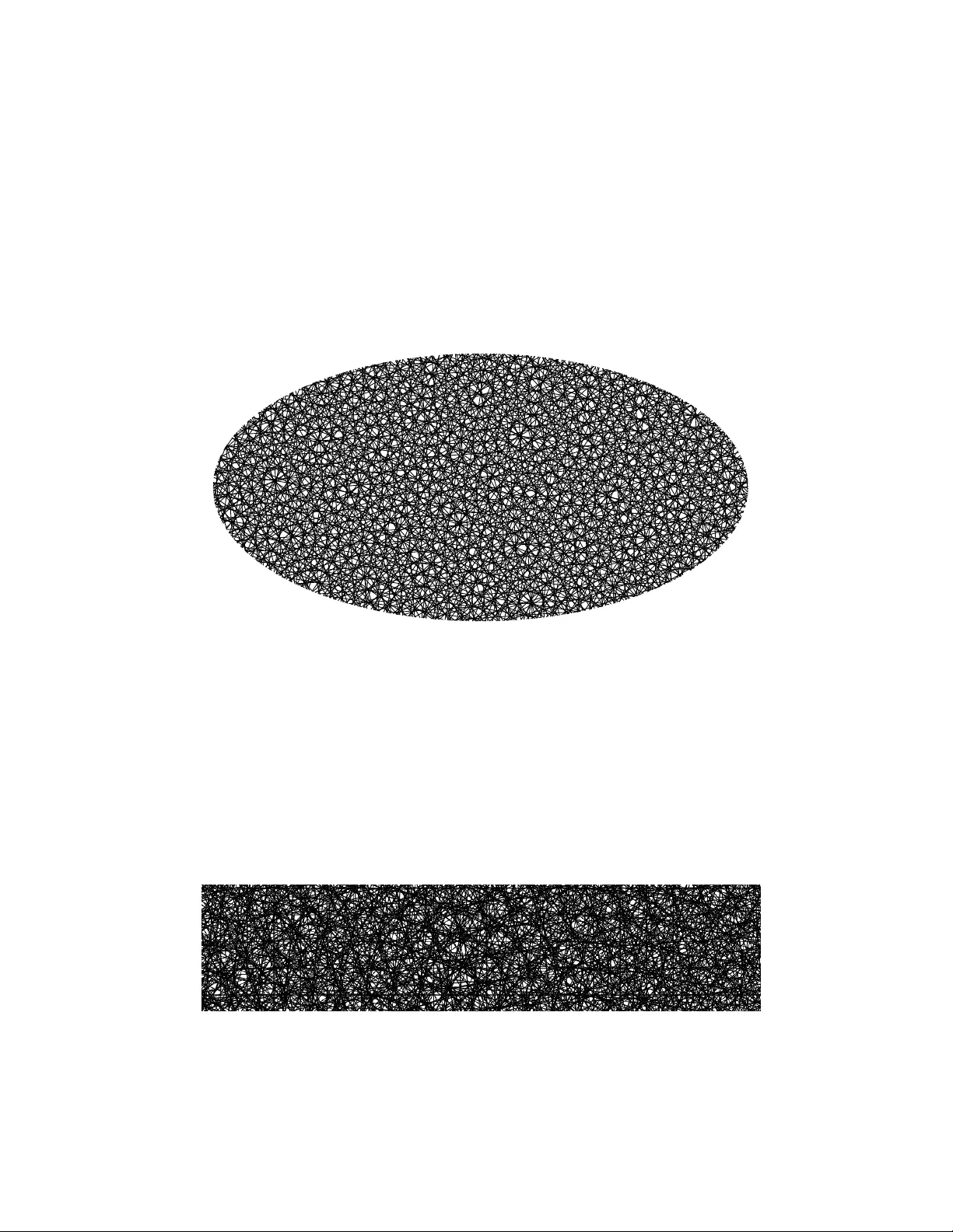
BUFF ON DISCREP ANCY AND THE STEINHA US LONGIMETER STEF AN STEINERBERGER Abstract. Let Ω ⊂ R 2 be a conv ex set. W e study the problem of distributing a one-dimensional set S with total length L so that for any line ℓ in R 2 the num b er of intersections #( ℓ ∩ S ) is prop ortional to the length H 1 ( ℓ ∩ Ω) as muc h as p ossible; w e use the term Buffon discrepancy for the largest error. A construction of Steinhaus can b e generalized to prov e the existence of sets with Buffon discrepancy ≲ L 1 / 3 . W e also sho w that the unit disk D admits a set with uniformly bounded Buffon discrepancy as L → ∞ . 1. Introduction 1.1. The problem. The goal of this pap er is to presen t an interesting problem: w e are given a b ounded, conv ex domain Ω ⊂ R 2 . The goal is to find, for any giv en L > 0, a one-dimensional set S ⊂ Ω with length L so that the follo wing is true: for an y line ℓ in R 2 the num ber of intersections #( ℓ ∩ S ) is proportional (as m uch as p ossible) to the length of the line inside Ω, that is H 1 ( ℓ ∩ Ω). The obvious questions are: ho w can this b e made precise, how well can it b e done and what do extremal sets S lo ok like? Computational exp erimen ts (see Fig. 1) suggest that the answer to these questions migh t be quite in teresting; the question is also of ob vious in terest in higher dimensions; this pap er is solely fo cused on the case of tw o dimensions. Figure 1. Sets of lines of length L = 500 inside the unit disk (left) and the Reuleaux triangle (right) with the prop ert y that ev ery line through the domain in tersects them a num b er of times roughly prop ortional to the length (with a fairly small error). 1 2 1.2. Buffon discrepancy. W e start by motiv ating the quantit y of in terest. Asking for the num b er of intersections to b e pr op ortional introduces t w o v ariables: (a) the prop ortionalit y factor and (b) the w orst case error assuming that proportionality factor. It is clear that these tw o num b ers (denoted c and X in the subsequent Prop osition) are highly connected and maybe one do es not wish to deal with b oth at the same time. Our first observ ation is that there exists a somewhat canonical prop ortionalit y factor c suggested b y the Cauch y-Crofton formula. Prop osition (Cauc h y-Crofton scaling) . L et Ω ⊂ R 2 b e b ounde d, let S b e a set with length H 1 ( S ) = L having the pr op erty that for some c > 0 and al l lines ℓ in R 2 #( ℓ ∩ S ) − c · H 1 ( ℓ ∩ Ω) ≤ X, then c − 2 π L area(Ω) ≤ 2 · diam(Ω) area(Ω) X. Since we are mainly in terested in the asymptotic regime L ≫ X , the Proposition suggests to pr escrib e the prop ortionalit y factor as 2 L/ ( π · area(Ω)). W e use this as our starting p oin t to define Buffon discrepancy . Definition. L et Ω ⊂ R 2 b e a b ounde d set in the plane and let S ⊂ Ω b e a r e ctifiable set with length L . We define the Buffon discrepancy of S (with r esp e ct to Ω ) as #( ℓ ∩ S ) − 2 π L area(Ω) H 1 ( ℓ ∩ Ω) L ∞ ( µ ) , wher e µ is the kinematic me asur e and ℓ r anges over al l lines. Note that if the set S w ere to con tain a line segment, then there exists a line ℓ such that #( ℓ ∩ S ) = ∞ . One could replace line segmen ts b y slightly curved segmen ts and tak e a limit but presumably the more natural w ay out is to exclude ‘exceptional lines of measure 0’ and this is done by the use of the kinematic measure; recall the formal definition of the L ∞ − norm as ∥ f ∥ L ∞ ( µ ) = inf { C ≥ 0 : | f ( x ) | ≤ C for µ almost every x } whic h encapsulates the idea that individual lines as well as sets of lines with measure 0 do not matter. 2000 line segments S with total length L = 500 the red line ℓ intersects #( ℓ ∩ S ) = 160 segmen ts and has length H 1 ( ℓ ) ∼ 1 . 769 160 − 2 L π 2 · 1 . 769 ∼ 19 . 24 Figure 2. A set with length L = 500 in the unit disk and a line sho wing that the Buffon discrepancy of the set is ≥ 19 . 24. 3 There exists a trivial lo wer b ound: for fixed Ω as L → ∞ , w e observe that the in tersection #( ℓ ∩ S ) is alw ays integer-v alued while the length of all chords assume in termediate real v alues; in general, we alw ays hav e a trivial b ound #( ℓ ∩ S ) − 2 π L area(Ω) H 1 ( ℓ ∩ Ω) L ∞ ( µ ) ≥ 1 2 . As it turns out, this trivial low er b ound is optimal in the case of the unit disk. 1.3. Unit Disk. The unit disk D is a natural first example. W e prov e the existence of a v ery simple set, a union of suitably placed concentric circles, with uniformly b ounded Buffon discrepancy . Theorem 1. F or any L > 0 ther e exists a set S ⊂ D with total length L with max ℓ #( ℓ ∩ S ) − 2 L π 2 H 1 ( ℓ ∩ D ) ≤ 100 . Figure 3. Tw o sets of line segmen ts with total length L = 500 inside the unit disk with very small Buffon discrepancy . It seems, see Fig. 1 and Fig. 3, that there are different t yp es of sets inside the unit disk that hav e a small Buffon discrepancy . The union of concentric circles is arguably the simplest one; how ev er, it migh t b e in teresting to see if it is p ossible to construct other examples of such sets. 1.4. The Steinhaus longimeter. This t ype of problem appears to b e very nat- urally related to a construction first prop osed (and patented!) by Hugo Steinhaus [23, 24, 25, 26]. His 1930 pap er On the pr actic e of r e ctific ation and notion of length [23] b egins by sa ying that This note b elongs to the area of applied mathematics. It prop oses a metho d whic h allows the optical measurement of ph ysically given curv es. The term ‘optical’ should highlight the distinction b et ween our metho d and the mechanical [...] There are many conceiv able cases where a mec hanical device cannot b e used. [...] for example if one wan ts to measure the length of a string-lik e curved ob ject under the microscop e [...] (Steinhaus, [23]) 4 One of the applications he has in mind is measuring the length of ob jects on a map as is also explained in his 1931 publication in Czasopismo Ge o gr aficzne (Geographic Journal) [24]. Steinhaus first explains the usual pro of of the Crofton formula and then notes that the pro of allows for a discretization: taking 6 lines with an angle of 30 degrees betw een them and all their translates, Steinhaus notes that the n umber of in tersections betw een this union of lines and an y line segmen t is nearly proportional to the length of the line segmen t up to an error b et ween − 2 . 26% and 1 . 15%. More generally , let S n,ε denote n lines going through the origin at an equal angle together with all translates by ε , S n,ε = cos ( π k/n ) sin ( π k/n ) t + − sin ( πk /n ) cos ( π k/n ) sε : t ∈ R , s ∈ Z , 0 ≤ k < n . The set S 1 ,ε is the union of lines parallel to the x − axis while S 2 ,ε is the familiar grid and S 3 ,ε leads to a hexagonal structure. The standard (patented) Steinhaus longimeter construction corresp onds to S 6 ,ε . Figure 4. The sets S n, 1 / 5 for 1 ≤ n ≤ 5. W e will now argue that this generalized Steinhaus longimeter provides a univ ersal b ound for our problem: as L → ∞ , the set S n,ε ∩ Ω, for suitable n, ε , is a set with small Buffon discrepancy . Theorem 2. L et Ω ⊂ R 2 b e a b ounde d, c onvex domain. Then ther e exists c Ω such that, as L → ∞ , the set S = Ω ∩ S L 1 / 3 ,L − 2 / 3 has length H 1 ( S ) ∼ L and #( ℓ ∩ S ) − 2 π L area(Ω) H 1 ( ℓ ∩ Ω) L ∞ ( µ ) ≤ c Ω · L 1 / 3 . It is not difficult to see that this result is sharp: the set Ω could b e oriented so that the origin (0 , 0) ∈ ∂ Ω. Ho w ev er, the Steinhaus set S n,ε has the prop ert y that n lines meet at the origin, therefore this b ound is the b est one can hop e for when n ∼ L 1 / 3 . One migh t naturally wonder whether it is p ossible to av oid this worst case scenario by suitably moving and rotating the set Ω, p erhaps an additional a veraging procedure can lead to a further impro vemen t. 1.5. Op en problems. These t w o results, a uniformly bounded Buffon discrepancy for the unit disk and a b ound of L 1 / 3 for general con v ex sets, naturally suggest a n umber of different questions. W e only list some of the more ob vious ones. (1) Is it alwa ys p ossible to find a set with Buffon discrepancy of order ∼ 1 for an y con v ex domain? If so, is there a simple construction? If not, what is the b est Buffon discrepancy one can hop e for? (2) Is it p ossible to find other explicit examples with Buffon discrepancy of order ∼ 1 for the unit disk? Fig.1 and Fig. 3 sho w n umerically obtained examples suggesting their existence. 5 (3) What happ ens if w e were to restrict ourselves to only working with sets S that are a union of in tersections of lines with Ω? This would include all Steinhaus sets but would eliminate examples lik e Fig. 3. W ould this fundamen tally change the problem? (4) What about the analogous problem in higher dimensions? Note that, for example in R 3 , there are at least tw o separate problems dep ending on whether ‘lines’ are understo o d to b e lines or sets of co-dimension 1. Figure 5. Construction in the style of the Steinhaus longimeter. It app ears as if Steinhaus sets are a fairly natural starting point when it comes to the construction of optimal sets; there are several natural v ariations one might w ant to consider, for example, we defined them to all meet in the origin but one could add an offset to each individual line to a v oid this cluster. A second interesting asp ect is that the Steinhaus sets S n,ε , esp ecially for n large and ε small, ha ve a fairly in triguing micro-structure (see, Fig. 6 and Fig. 7). There are regions that app ear fairly random, there are obvious clusters where many lines meet and there are some relatively empty regions. Theorem 2 suggests that S n, 1 /n 2 for n ∈ N might b e a particularly in teresting subfamily . Figure 6. Microstructures in S 50 , 1 / 2500 . 6 1.6. Related results. W e are not a w are of any directly related results in integral geometry [22]. Our problem can b e understo od in the spirit of discrepancy theory , see Bec k-Chen [4], Chazelle [6], Drmota-Tich y [10], Kuipers-Niederreiter [15] and Matousek [19]. Indeed, it could b e interpreted as the problem finding a suitable discretization of kinematic measure restricted to a domain, how ev er, w e know of no w ork in that direction. The Steinhaus longimeter has had profound impact in ster e olo gy , the study of how to extract information from low er-dimensional sets, we refer to [3, 5, 7, 8, 9, 11, 12, 13, 16]. A related result is due to Liu-Zhang-Zheng- P aul [17]: they use a lo w-discrepancy sequence on the sphere to create ‘uniformly distributed’ lines, though, in their setup the goal is surface estimation of an a priori unkno wn ob ject. This has since b een further pursued [14, 21], how ev er, it is really a different problem. W e also note the existence of the work of Ambartzumian [1, 2] whic h, again, seems to b e of a very differen t flav or. 2. Proofs 2.1. Pro of of the Prop osition. Pr o of. Since Ω is b ounded, we may assume without loss of generality that it is con tained in a ball of radius R cen tered at the origin, i.e. Ω ⊂ B (0 , R ). W e will no w consider the set of all lines ℓ that in tersect this ball which we can iden tify with the in terv al [ − R, R ] × S 1 equipp ed with the usual pro duct measure: this iden tifies each line with the angle that it makes with the x − axis (or any other fixed reference direction) as w ell as the closest (signed) distance it has with the origin. By choosing the pro duct measure, the arising measure is in v ariant under rotation and translation. This set has total measure 2 R × 2 π = 4 Rπ . Since the set S is rectifiable, we ma y think of it as a union of finitely many line segments; we first argue that linearity gives that Z R − R Z 2 π 0 #( ℓ ∩ S ) dxdθ = 4 L. This can be seen as follo ws: if S is a line segmen t of length ε , then the size of its pro jection depends on the angle α b et ween the pro jection direction and the orien tation of the line segment and ev aluates to | cos α | ε . In that case, Z R − R Z 2 π 0 #( ℓ ∩ S ) dxdθ = Z 2 π 0 Z R − R #( ℓ ∩ S ) dxdθ = Z 2 π 0 | cos α | εdα = 4 ε. Since the integral is additive, we arriv e at the desired conclusion. Simultaneously , b y F ubini, we hav e Z R − R Z 2 π 0 H 1 ( ℓ ∩ Ω) dxdθ = Z 2 π 0 Z R − R H 1 ( ℓ ∩ Ω) dxdθ = Z 2 π 0 area(Ω) dθ = 2 π · area(Ω) . If it is now true that for some c, X > 0 and all lines ℓ w e hav e that #( ℓ ∩ S ) − c · H 1 ( ℓ ∩ Ω) ≤ X, 7 then the triangle inequality implies | 4 L − c · 2 π · area(Ω) | = Z R − R Z 2 π 0 #( ℓ ∩ S ) − c · H 1 ( ℓ ∩ Ω) dxdθ ≤ Z R − R Z 2 π 0 #( ℓ ∩ S ) − c · H 1 ( ℓ ∩ Ω) dxdθ ≤ 4 π RX . Dividing b oth sides b y 2 π area(Ω) no w leads to c − 2 π L area(Ω) ≤ 2 R area(Ω) X. Using R ≤ diam(Ω) implies the result. □ Figure 7. Pictures at an exhibition: S 50 , 1 / 2500 at small scale. 2.2. Pro of of Theorem 1. Pr o of. W e consider a union of circles centered at the origin. More precisely , given radii 0 < r 1 < r 2 < · · · < r k ≤ 1, we consider the set S = k [ i =1 x ∈ R 2 : ∥ x ∥ = r i . The length of this set is supp osed to b e L , this requires r 1 + r 2 + · · · + r k = L 2 π . F or any arbitrary line ℓ , w e consider its closest approach to the origin, i.e. d ( ℓ ) = min x ∈ ℓ ∥ x ∥ . Then H 1 ( ℓ ∩ D ) = 2 p 1 − d ( ℓ ) 2 . Sim ultaneously , we hav e that, except for a set of kinematic measure 0 #( S ∩ ℓ ) = 2 · # { 1 ≤ i ≤ k : d ( ℓ ) ≤ r i } . The exceptional set of lines is exactly the set of lines that is tangent to one of the k circles and this tells us that for al l lines | #( S ∩ ℓ ) − 2 · # { 1 ≤ i ≤ k : d ( ℓ ) ≤ r i }| ≤ 1 . 8 W e arriv e at the b ound #( ℓ ∩ S ) − 2 L π 2 H 1 ( ℓ ∩ D ) ≤ 1 + 2 · # { 1 ≤ i ≤ k : d ( ℓ ) ≤ r i } − 2 L π 2 H 1 ( ℓ ∩ D ) ≤ 1 + 2 # { 1 ≤ i ≤ k : d ( ℓ ) ≤ r i } − 2 L π 2 p 1 − d ( ℓ ) 2 . The line ℓ has b een reduced to a num b er 0 < d ( ℓ ) < 1 and it remains to find a suitable k ∈ N and a suitable set of k radii r 1 < r 2 < · · · < r k sub ject to the b oundary conditions indicated ab o ve such that max 0
Original Paper
Loading high-quality paper...
Comments & Academic Discussion
Loading comments...
Leave a Comment