GSW: Generalized "Self-Wiener" Denoising

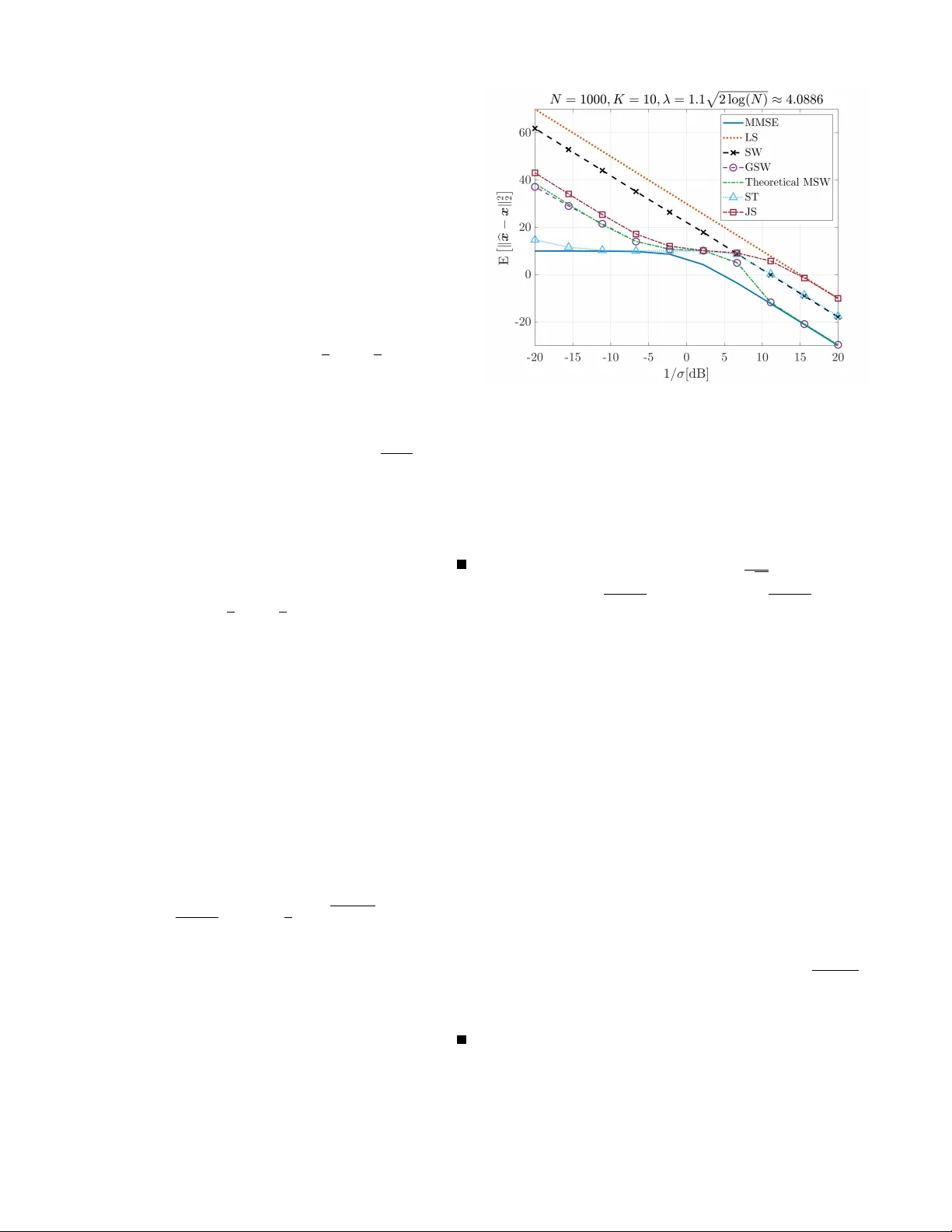
1 GSW : Generalized “Self-W iener” Denoising Amir W eiss Faculty of Engineering Bar-Ilan Uni versity Ramat-Gan, Israel amir .weiss@biu.ac.il Abstract —W e revisit the recently proposed “self-Wiener” (SW) filtering method for r obust decon volution, and generalize it to the classical denoising problem. The resulting estimator , termed generalized SW (GSW) filtering, retains the nonlinear shrinkage structur e of SW but introduces a tunable threshold parameter . This tunability enables GSW to flexibly adapt to varying signal-to-noise ratio (SNR) regimes by balancing noise suppression and signal preserv ation. W e derive closed-form expressions f or its mean-square error (MSE) perf ormance in both low- and high-SNR regimes, and demonstrate that GSW closely approximates the oracle MMSE at high SNR while maintaining strong robustness at low SNR. Simulation results validate the analytical findings, showing that GSW consistently achiev es fav orable denoising performance across a wide range of SNRs. Its analytical tractability , parameter flexibility , and close connection to the optimal Wiener filter structur e make it a promising tool f or practical applications including compr essive sensing, sparse signal r ecovery , and domain-specific shrinkage in wav elet, Fourier , and potentially learned orthonormal representations. Index T erms —Denoising, thresholding, Wiener filter . I . I N T R O D U CT I O N Denoising remains a fundamental task in signal processing, with broad relev ance across domains such as communications, imaging, and geophysical sensing (e.g., [1]–[5]). In many ap- plications, one ultimately needs accurate estimates of a signal- of-interest (SOI) from noisy measurements due to physical effects of additi ve noise, either directly in the domain they were measured (e.g., time or space) or after a transform (e.g., Fourier or wav elet [6]) to a more conv enient, or in some sense more natural, representation. Classical approaches range from linear W iener filtering [7]—optimal under Gaussian statisti- cal models with known second-order statistics—to nonlinear shrinkage and thresholding methods designed for sparse or compressible representations [8]–[10]. A recent contribution in this broader space is the “self- W iener” (SW) filter [11], originally proposed for robust decon- volution of deterministic signals. There, under an approximate independence assumption between discrete Fourier transform (DFT) components, SW applies a nonlinear thershold-type shrinkage operator to each DFT coefficient of the decon volved signal. Analytically , it was shown that in the high signal- to-noise ratio (SNR) regime, this nonlinear operator closely approximates the ideal (but unrealizable) Wiener filter , while at lo w SNR it acts as an aggressiv e noise suppressor . Howe ver , the original SW formulation, which was tailored to decon volution with a known linear time-inv ariant system, uses a fixed threshold value. This limits its adaptability when applied to pure denoising problems, where one typically has more freedom in choosing the operating point, and where transform-domain sparsity or compressibility can often be exploited explicitly . In particular, in low SNR regimes there is a benefit in allowing the user to bias the estimator toward stronger noise suppression, whereas at high SNR one would like to remain as close as possible to the oracle minimum mean-square error (MMSE) solution, or at least to the oracle linear MMSE solution, obtained via Wiener filtering. In this work, we revisit the core SW idea from a de- noising vie wpoint and specialize it to the canonical additive white Gaussian noise (A WGN) model. The resulting estimator , which we term generalized self-W iener (GSW) filtering, re- tains the scalar , coefficient-wise nonlinear shrinkage structure of SW but introduces an explicit tunable threshold parameter . This tunability allows GSW to interpolate between an ag- gressiv ely regularized, highly robust regime and a near-oracle MMSE regime, and makes it directly applicable as a drop-in shrinkage rule in generic orthonormal representations, such as Fourier , wavelet, and potentially learned transforms. Our ke y contributions in this work are the following: • GSW filtering for denoising: W e introduce a tunable generalization of the SW filter [11] for the standard A WGN denoising problem. GSW preserves the Wiener - like shrinkage structure of SW but adds flexibility in the threshold parameter that can be matched to the noise lev el or chosen according to classical prescriptions (e.g., univ ersal or SURE-based thresholds [8], [12]). • Analytical performance char acterization: W e derive closed-form expressions for the mean-square error (MSE) of GSW in both lo w- and high-SNR regimes and show that, for appropriate threshold choices, GSW closely tracks the oracle MMSE at high SNR while maintaining strong robustness and noise suppression at lo w SNR. • Empirical validation and comparison: W e compare the GSW to established benchmarks such as the least-squares (LS) estimator , James–Stein (JS) shrinkage [13], and soft-thresholding (ST) [9] in a simulation experiment on synthetic data in a sparse vector denoising task, and demonstrate that GSW provides competitive or superior performance across a wide range of noise conditions. The rest of the paper is organized as follo ws. Section II formalizes the denoising problem. Section III introduces the GSW estimator and presents the MSE performance analysis in the low- and high-SNR regimes. Section IV provides numerical simulations, and Section V concludes the paper . 2 I I . P R O B L E M F O R M U L A T I O N W e consider the canonical signal-plus-noise model y = x + σ ξ ∈ C N × 1 , (1) where x ∈ C N × 1 is an unknown deterministic SOI, ξ ∼ C N ( 0 , I N ) is an standard, circularly symmetric complex normal vector with independent entries, and σ ∈ R + denotes the noise standard deviation. 1 Thus, componentwise, y n = x n + σ ξ n , n = 1 , . . . , N , (2) with ξ n ∼ C N (0 , 1) . This model also covers transform-domain denoising under any unitary transform U ∈ C N × N : setting ˜ y ≜ U H y and ˜ x ≜ U H x yields ˜ y = ˜ x + σ ˜ ξ , (3) with ˜ ξ ∼ C N ( 0 , I N ) by unitary inv ariance. Hence, without loss of generality , we may regard y as either a time-/space- domain vector or a collection of transform coefficients and focus on estimators that act componentwise on { y n } N n =1 . Our goal is to estimate x from its noisy observation y by means of an estimator b x = b x ( y ) , and to ev aluate its performance via the MSE, MSE ( x , b x ) ≜ E  ∥ b x ( y ) − x ∥ 2 2  (4) = N X n =1 E  | ˆ x n ( y n ) − x n | 2  , (5) where the expectation is with respect to the noise ξ , and in the second equality we have emphasized the scalar , compo- nentwise form of the estimator, ˆ x n = ˆ x n ( y n ) , that will be the focus of this work. W e also define the per-component SNR, SNR ( x n , σ ) ≜ | x n | 2 σ 2 , (6) and we will use the terms “lo w-SNR” and “high-SNR” regimes to refer to the limits SNR ( x n , σ ) → 0 and SNR ( x n , σ ) → ∞ , respectiv ely . T o keep the exposition simple, we assume homoscedastic noise throughout, i.e., ξ ∼ C N ( 0 , I N ) . The extension to a heteroscedastic noise ξ ∼ C N ( 0 , Λ ) , with a positive-definite diagonal covariance Λ ≻ 0 , is straightforward and does not alter the core analysis, provided the noise variances are known or can be estimated and appropriately normalized per component. I I I . G E N E R A L I Z E D “ S E L F - W I E N E R ” F I L T E R I N G In this section, we introduce GSW filtering, or the GSW estimator , for model (2). W e first define the estimator as a nonlinear shrinkage of the LS solution and then analyze its MSE in the high- and low-SNR regimes. 1 Throughout the paper, all randomness is due to the noise ξ ; the SOI x is treated as deterministic. A. Definition and Intuition It is well known that, under the model y = x + σ ξ , the LS (and maximum-likelihood) estimator of x is giv en by b x LS ≜ y . (7) Building on the structure of the SW filter [11, Eq. (17)], we define the generalized SW (GSW) estimator as a nonlinear shrinkage of the LS estimate, parameterized by a tunable threshold λ ∈ [2 , ∞ ) . Specifically , the GSW estimator of the n -th entry of x is given by b x n, GSW ≜ y n ·      2 | z n | − 2 1 − p 1 − 4 | z n | − 2 , | z n | > λ, 0 , | z n | ≤ λ, (8) where z n ≜ y n σ = x n σ + ξ n ≜ η n + ξ n , n = 1 , . . . , N , (9) and η n ≜ x n /σ is the (complex-v alued) signal normalized by the noise standard deviation. In particular, we have | η n | 2 = SNR ( x n , σ ) , (10) thus, | z n | 2 is an estimator of the SNR of the n -th coordinate. One may view (8) as applying a scalar shrinkage factor g λ ( · ) to the LS estimate: b x n, GSW = b x n, LS · g λ ( | z n | ) , (11) where g λ ( r ) ≜      2 r − 2 1 − √ 1 − 4 r − 2 , r > λ, 0 , r ≤ λ, r ≥ 0 . (12) Remark 1 (Relation to the original SW estimator): The original SW estimator [11] corresponds to the special case λ = 2 in (8). This choice yields a parameter-free, robust estimator that was shown to approximate the ideal Wiener filter in the high-SNR regime for the decon volution setting. In the general denoising problem, ho wever , fixing λ = 2 may be suboptimal at low SNR, where stronger noise suppression can be desirable. GSW introduces λ as a tunable parameter, allowing to trade of f bias and variance across SNR regimes. The intuition behind (8) is as follo ws. The GSW rule applies a nonlinear shrinkage factor that aggressively zeroes out low- SNR components (those for which | z n | ≤ λ ) while preserving and gracefully attenuating components above the threshold. Compared to classical thresholding, GSW has a more nuanced, data-dependent shrinkage profile that preserves a Wiener -like structure for large | z n | and provides additional robustness through the tunable parameter λ . Indeed, when | η n | → ∞ , we hav e | z n | → ∞ almost surely , hence 2 | z n | − 2 1 − p 1 − 4 | z n | − 2 = 1 1 + | z n | − 2 + O p ( | z n | − 4 ) (13) = ⇒ b x n, GSW ≈ b x n, LS · SNR ( x n , σ ) 1 + SNR ( x n , σ ) , (14) i.e., the oracle MMSE solution. 2 2 Oracle, and not realizable, since we recall that SNR ( x n , σ ) is a function of x n , which is unknown. 3 B. Asymptotic MSE Analysis W e now analyze the elementwise MSE of b x n, GSW (8), MSE n ( η n , λ ) ≜ E î | b x n, GSW − x n | 2 ó , (15) as a function of the normalized signal η n = x n /σ and the threshold λ . Our focus is on asymptotic expressions in the high- and low-SNR regimes, i.e., | η n | → ∞ and | η n | → 0 , respectiv ely . 1) High-SNR re gime: In the high-SNR regime, the GSW estimator behaves as a perturbed oracle MMSE solution. The following result formalizes this behavior . Pr oposition 1 (High-SNR performance): Let z n be as in (9) and define p n ≜ Pr ( | z n | > λ ) = Q 1 Ä √ 2 | η n | , √ 2 λ ä , (16) where Q 1 ( · , · ) is the Marcum Q -function [14]. Then, for | η n | ≫ λ , the MSE of the estimator (8) admits the expansion MSE n ( η n , λ ) = (1 − p n ) | x n | 2 + p n σ 2 + O Å σ 2 | η n | 2 ã . (17) Pr oof sketch: A detailed deri vation is provided in Ap- pendix A. The proof proceeds by conditioning on the ev ents {| z n | ≤ λ } and {| z n | > λ } , exploiting the noncentral χ 2 distribution of | z n | 2 , and performing a high-SNR expansion in po wers of | η n | − 1 . The interpretation of Proposition 1 is that, at high SNR, the GSW estimate closely approximates the oracle MMSE solution. Indeed, Q 1 Ä √ 2 | η n | , √ 2 λ ä → 1 as | η n | → ∞ , so the leading term in (17) tends to σ 2 , which is the MSE of the LS estimator in this deterministic setting, and the asymptotic MSE of the oracle MMSE solution. The probability of erroneously shrinking the coefficient to zero v anishes exponentially fast with | η n | 2 , and the term O ( σ 2 / | η n | 2 ) becomes negligible. 2) Low SNR r egime: In the low SNR regime, the dominant challenge is noise suppression. The next result characterizes the residual noise variance induced by the GSW rule (8). Pr oposition 2 (Low-SNR performance): For entries with low SNR, i.e., | η n | ≪ 1 , the MSE of the GSW estimator satisfies MSE n ( η n , λ ) = | x n | 2 + ρ GSW ( λ ) σ 2 + O ( | η n | ) , (18) where p n = Pr( | z n | > λ ) as in (16) and ρ GSW ( λ ) ≜ Å λ 2 − 1 2 ã e − λ 2 + 1 2 ∞ Z λ 2 p t 2 − 4 t e − t d t. (19) Pr oof sketch: A detailed deri vation is provided in Ap- pendix B. The proof relies on expanding the noncentral χ 2 density of | z n | 2 around η n = 0 , ev aluating the resulting inte- grals term by term, and isolating the leading-order contribution to the residual variance as a function of λ . Proposition 2 shows that, at low SNR, GSW effecti vely sup- presses noise by pushing most coefficients below the threshold while controlling the residual variance through ρ GSW ( λ ) . For suitably chosen λ , ρ GSW ( λ ) can be significantly smaller than the unit variance of the LS estimator , as ρ GSW ( λ ) − − − − → λ →∞ 0 , leading to substantial gains over naiv e denoising strategies. Fig. 1: MSE versus in verse noise RMS power for a sparse signal with K = 10 non-zero entries (unit magnitude) out of N = 1000 . Results are averaged o ver 10 3 realizations. GSW approaches the oracle MMSE bound at high SNR and outperforms LS, JS, ST , and SW at medium-to-high SNR. Remark 2 (Real-valued case): Propositions 1 and 2 extend naturally to the real-valued case, where x ∈ R N × 1 and ξ ∼ N ( 0 , I N ) . In that setting, p n = Q ( λ − η n ) + Q ( λ + η n ) , where Q ( x ) ≜ R ∞ x φ ( t ) d t with φ ( x ) ≜ 1 √ 2 π e − x 2 / 2 , and ρ GSW ( λ ) ≜ Ä λ + p λ 2 − 4 ä φ ( λ ) + e − 2 Q Ä p λ 2 − 4 ä − Q ( λ ) . (20) The qualitati ve conclusions reg arding the behavior of the GSW estimator remain unchanged. The high- and low-SNR regimes characterizations above highlight the role of GSW as a flexible nonlinear shrinkage es- timator that balances signal preservation and noise suppression through the tunable parameter λ . In Section IV, we compare GSW to classical established benchmarks in a simulation experiment of a generic sparse vector denoising scenario. I V . S I M U L AT I O N R E S U LT S W e illustrate the behavior of GSW in sparse vector denois- ing. The signal x has K = 10 non-zero entries (each of unit magnitude) out of N = 1000 coordinates. For each noise lev el, the empirical MSE is averaged ov er 10 3 independent realizations. Figure 1 sho ws the MSE versus the in verse noise variance 1 /σ 2 (equiv alently , in this case, SNR ( x n , σ ) ). W e compare GSW (8) to LS (7), ST [9], JS [13], the original SW estimator [11], and the MMSE oracle lo wer bound from [11, Eq. (13)]. The threshold is set to λ = 1 . 1 √ 2 log N ≈ 4 . 09 , a slightly inflated universal threshold [9, Eq. (32)]. Evidently , GSW achieves in this setting a f avorable trade-of f across SNR regimes: it closely tracks the MMSE at high SNR while providing robust denoising at low SNR. In particular: • ST performs best among the classical thresholding rules at very low SNR, b ut GSW overtak es it around ∼ 2 dB and maintains a noticeable advantage thereafter . • GSW improv es upon SW and JS across the entire SNR range, demonstrating the benefit of threshold tunability . 4 V . C O N C L U S I O N W e have introduced GSW filtering as a tunable-threshold- type shrinkage rule for A WGN denoising, extending the origi- nal SW estimator from decon volution to the canonical signal- plus-noise model. GSW preserves the W iener-lik e structure at high SNRs while enjoying an additional de gree of freedom in the form of a threshold parameter that enables a controlled trade-off between bias and variance across SNR regimes. W e deriv ed closed-form high- and low-SNR MSE expressions, showing that GSW approaches the oracle MMSE performance at high SNR and achie ves effecti ve noise suppression at low SNR through the parameter-dependent constant ρ GSW ( λ ) . Simulations on a generic sparse denoising problem confirm these properties and demonstrate improvements over LS, JS, ST , and the original SW rule. These results suggest that GSW is a useful building block for practical transform-domain de- noising, including sparse and other structured signal settings. A P P E N D I X A P RO O F O F P R OP O S I T I O N 1 W e consider a single coordinate and omit the index n . Recall that y = x + σ ξ , z = y σ = η + ξ , (21) with ξ ∼ C N (0 , 1) and η ≜ x/σ . The scalar GSW estimate is b x GSW = y g λ ( | z | ) = σ ( η + ξ ) g λ ( | z | ) , (22) where g λ ( · ) is gi ven by (12). Define A ≜ {| z | ≤ λ } , A c ≜ {| z | > λ } , (23) and p ≜ Pr ( A c ) = Pr( | z | > λ ) = Q 1 Ä √ 2 | η | , √ 2 λ ä . (24) Using the indicator function 1 {·} , the MSE decomposes as E  | b x GSW − x | 2  = E  | b x GSW − x | 2 1 A  (25) + E  | b x GSW − x | 2 1 A c  . (26) Giv en A , we hav e b x GSW = 0 , hence E  | b x GSW − x | 2 1 A  = | x | 2 Pr( A ) = (1 − p ) | x | 2 . (27) Giv en A c , b x GSW is given by (22) with | z | > λ , and we can write the error as b x GSW − x = σ z g λ ( | z | ) − x. (28) Thus E  | b x GSW − x | 2 1 A c  = σ 2 E  | z g λ ( | z | ) | 2 1 A c  + p | x | 2 (29) − 2 σ ℜ { x ∗ E [ z g λ ( | z | ) 1 A c ] } . (30) W e now isolate the leading 1 / | z | 2 behavior of g λ ( · ) . Using g λ ( r ) = 2 r − 2 1 − √ 1 − 4 r − 2 = 1 2 Ä 1 + p 1 − 4 r − 2 ä , r > 2 , (31) a second-order T aylor expansion of √ 1 − 4 r − 2 around r − 2 = 0 yields g λ ( r ) ≜ 1 − 1 r 2 + δ λ ( r ) , (32) with a remainder term satisfying | δ λ ( r ) | ≤ C λ r 4 , r ≥ λ, (33) for some finite constant C λ that depends on λ but not on η or σ . Substituting g λ ( | z | ) = 1 − | z | − 2 + δ λ ( | z | ) into (29), we first expand the two expectations that appear there. On A c , z g λ ( | z | ) = z Å 1 − 1 | z | 2 + δ λ ( | z | ) ã = z − z | z | 2 + z δ λ ( | z | ) , (34) and | z g λ ( | z | ) | 2 (35) = | z | 2 Å 1 − 1 | z | 2 + δ λ ( | z | ) ã Å 1 − 1 | z | 2 + δ λ ( | z | ) ã ∗ (36) ≜ | z | 2 − 2 + r λ ( z ) , (37) where, for some constant K λ < ∞ , | r λ ( z ) | ≤ K λ | z | 2 , | z | ≥ λ. (38) Using (34) we have E [ z g λ ( | z | ) 1 A c ] = E [ z 1 A c ] − E ï z | z | 2 1 A c ò (39) + E [ z δ λ ( | z | ) 1 A c ] , (40) and from the expression for | z g λ ( | z | ) | 2 , E  | z g λ ( | z | ) | 2 1 A c  = E  | z | 2 1 A c  − 2 p + E [ r λ ( z ) 1 A c ] . (41) W e now use asymptotic expansions of the v arious terms as | η | → ∞ . Recall z = η + ξ with ξ ∼ C N (0 , 1) . Then E [ z ] = η , E [ | z | 2 ] = | η | 2 + 1 . (42) Moreov er, the e vent {| z | ≤ λ } lies in a fixed ball around the origin, while z is centered at η , hence there exist constants c, C > 0 such that Pr( A ) = Pr( | z | ≤ λ ) ≤ C e − c | η | 2 , | η | → ∞ . (43) Since E [ f ( z ) 1 A c ] = E [ f ( z )] − E [ f ( z ) 1 A ] , it follo ws that E [ z 1 A c ] = η + O Ä e − c | η | 2 ä , (44) E  | z | 2 1 A c  = | η | 2 + 1 + O Ä e − c | η | 2 ä , (45) p = 1 + O Ä e − c | η | 2 ä . (46) Next, we bound the terms in volving | z | − 2 and δ λ ( · ) . For | z | ≥ λ , from (33), we hav e | z δ λ ( | z | ) | ≤ C λ | z | 3 , | r λ ( z ) | ≤ K λ | z | 2 . (47) Similarly to the technique in [11, Lemma 1], using T aylor expansions around z = η , one obtains E ï z | z | 2 1 A c ò = 1 η ∗ + O Å 1 | η | 3 ã , (48) E [ z δ λ ( | z | ) 1 A c ] = O Å 1 | η | 3 ã , (49) E [ r λ ( z ) 1 A c ] = O Å 1 | η | 2 ã , (50) 5 as | η | → ∞ by using that ξ has finite moments of all orders and that Pr( A ) (in (43)) is exponentially small in | η | . Substituting (44), (48), and (49) into (40), and recalling x = σ η , we get E [ z g λ ( | z | ) 1 A c ] = η − 1 η ∗ + O Å 1 | η | 3 ã , (51) and hence − 2 σ ℜ { x ∗ E [ z g λ ( | z | ) 1 A c ] } (52) = − 2 σ ℜ ß ( σ η ) ∗ Å η − 1 η ∗ ã™ + O Å σ 2 | η | 2 ã (53) = − 2 | x | 2 + 2 σ 2 + O Å σ 2 | η | 2 ã . (54) Similarly , substituting (45), (46), and (50) into (41) yields E  | z g λ ( | z | ) | 2 1 A c  = | η | 2 − 1 + O Å 1 | η | 2 ã , (55) and therefore σ 2 E  | z g λ ( | z | ) | 2 1 A c  = | x | 2 − σ 2 + O Å σ 2 | η | 2 ã . (56) Combining (54), (56) and p | x | 2 = | x | 2 + O Å σ 2 | η | 2 ã , (57) σ 2 = pσ 2 + (1 − p ) σ 2 = pσ 2 + O Ä e − c | η | 2 ä , (58) in (30), we obtain E  | b x GSW − x | 2 1 A c  = p σ 2 + O Å σ 2 | η | 2 ã . (59) Substituting (27) and (59) into the decomposition (26) yields E  | b x GSW − x | 2  = (1 − p ) | x | 2 + p σ 2 + O Å σ 2 | η | 2 ã , (60) which is precisely (17) in Proposition 1. A P P E N D I X B P RO O F O F P R OP O S I T I O N 2 W e again work with a single coordinate, omit the index n and use the same definitions as in Appendix A. Recall the MSE decomposition E  | b x GSW − x | 2  = (1 − p ) | x | 2 + p E  | b x GSW − x | 2 | A c  . (61) Since z ∼ C N ( η , 1) , the probability p = Pr( | z | > λ ) is analytic in | η | and, expanding around η = 0 , we obtain (cf. [11, Eq. (50)–(51)]) p = p 0 + O  | η | 2  , p 0 ≜ Pr( | ξ | > λ ) ∈ (0 , 1) . (62) Write the conditional MSE conditioned on A c as E  | b x GSW − x | 2 | A c  = | x | 2 + σ 2 E  | z g λ ( | z | ) | 2 | A c  (63) − 2 σ 2 ℜ { η ∗ E [ z g λ ( | z | ) | A c ] } . (64) Since the map η 7→ E [ z g λ ( | z | ) | A c ] is analytic, we may write it (near η = 0 ) as E [ z g λ ( | z | ) | A c ] = E [ z g λ ( | z | ) | A c ] | η =0 + O ( | η | ) . (65) Howe ver , at η = 0 the distrib ution of z is rotationally symmetric ( z | η =0 = ξ ∼ C N (0 , 1) ) while g λ ( | z | ) depends only on | z | . Hence E [ z g λ ( | z | ) | A c ] | η =0 = 0 ⇒ E [ z g λ ( | z | ) | A c ] = O ( | η | ) , (66) so the cross term in (64) contributes O ( | x | | η | ) = O ( | η | 2 ) . Proceeding to the second term in (63), we have σ 2 E  | z g λ ( | z | ) | 2 | A c  (67) = σ 2 E  | ξ | 2 | g λ ( | ξ | ) | 2 | | ξ | > λ  + O ( | η | ) (68) = σ 2 · ρ GSW ( λ ) p 0 + O ( | η | ) , (69) where, by explicit radial integration (see [11, Appendix A]), we obtain the constant (19), which depends only on λ . Substituting (66) and (69) into (64) gives E  | b x GSW − x | 2 | A c  = | x | 2 + ρ GSW ( λ ) σ 2 + O ( | η | ) . (70) Finally , inserting this and (62) into (61) yields E  | b x GSW − x | 2  = (1 − p ) | x | 2 (71) + p Å | x | 2 + σ 2 · ρ GSW ( λ ) p 0 + O ( | η | ) ã (72) = | x | 2 + σ 2 · ρ GSW ( λ ) + O ( | η | ) , (73) which is the claimed low-SNR expansion (18). R E F E R E N C E S [1] A. Buades, B. Coll, and J.-M. Morel, “ A non-local algorithm for image denoising, ” in Proceedings of the 2005 IEEE Computer Society Confer ence on Computer V ision and P attern Recognition (CVPR’05) , 2005, pp. 60–65. [2] J. Benesty , J. Chen, Y . Huang, and I. Cohen, Noise Reduction in Speech Pr ocessing , vol. 2, Springer Science & Business Media, 2009. [3] P . C. Loizou, Speech Enhancement: Theory and Practice , CRC Press, 2 edition, 2013. [4] H. Meyr , M. Moeneclaey , and S. A. Fechtel, Digital communication r eceivers: synchr onization, channel estimation, and signal processing , vol. 444, Wiley Online Library , 1998. [5] C. Schmelzbach and E. Huber , “Ef ficient decon volution of ground- penetrating radar data, ” IEEE T rans. Geosci. Remote Sens. , vol. 53, no. 9, pp. 5209–5217, 2015. [6] S. Mallat, A W avelet T our of Signal Pr ocessing: The Sparse W ay , Academic Press, Amsterdam, 3 edition, 2009. [7] N. Wiener , Extrapolation, Interpolation, and Smoothing of Stationary T ime Series: W ith Engineering Applications , MIT Press, Cambridge, MA, 1949. [8] D. L. Donoho and I. M. Johnstone, “Ideal spatial adaptation by wavelet shrinkage, ” biometrika , vol. 81, no. 3, pp. 425–455, 1994. [9] D. L. Donoho, “De-noising by soft-thresholding, ” IEEE T rans. Inf. Theory , vol. 41, no. 3, pp. 613–627, 1995. [10] K. Dabov , A. F oi, V . Katkovnik, and K. Egiazarian, “Image denoising by sparse 3-D transform-domain collaborative filtering, ” IEEE T rans. Image Pr ocess. , vol. 16, no. 8, pp. 2080–2095, 2007. [11] A. W eiss and B. Nadler, ““Self-Wiener” filtering: Data-driven deconvo- lution of deterministic signals, ” IEEE T rans. Signal Process. , vol. 70, pp. 468–481, 2021. [12] F . Luisier , T . Blu, and M. Unser, “ A new SURE approach to image denoising: Interscale orthonormal wa velet thresholding, ” IEEE T rans. Image Pr ocess. , vol. 16, no. 3, pp. 593–606, 2007. [13] N. R. Draper and R. C. V an Nostrand, “Ridge regression and James- Stein estimation: revie w and comments, ” T echnometrics , vol. 21, no. 4, pp. 451–466, 1979. [14] G. E. Corazza and G. Ferrari, “New bounds for the Marcum Q-function, ” IEEE Tr ans. Inf. Theory , vol. 48, no. 11, pp. 3003–3008, 2002.