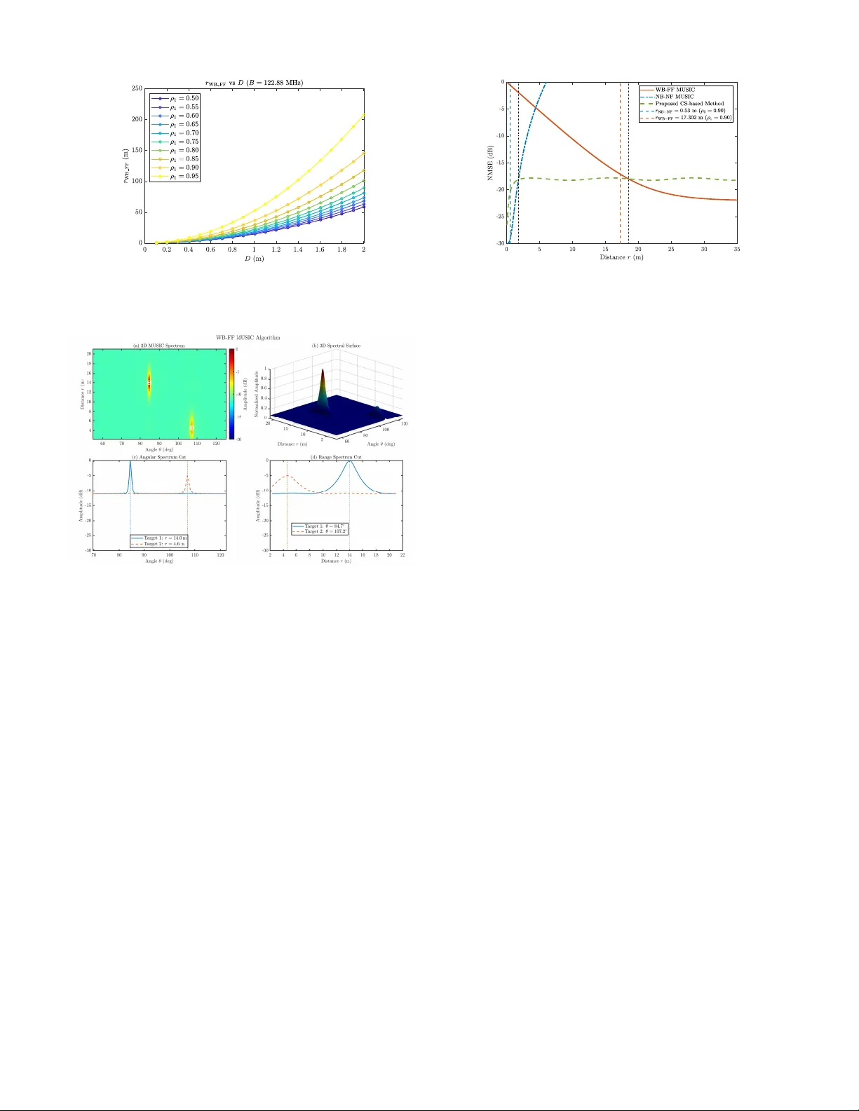
Wideband Near-Field Sensing in ISAC: Unified Algorithm Design and Decoupled Effect Analysis

1 W ideband Near -Field Sensing in ISA C: Unified Algorithm Design and Decoupled Ef fect Analysis Ruiyun Zhang, Zhaolin W ang, Zhiqing W ei, Y uanwei Liu, Zehui Xiong, Zhiyong Feng Abstract —T o advance integrated sensing and communications (ISA C) in sixth-generation (6G) extremely large-scale multiple- input multiple-output (XL-MIMO) networks, a low-complexity compressed sensing (CS)-based dictionary design is proposed for wideband near-field (WB-NF) target localization. Currently , the massive signal dimensions in the WB-NF regime impose sever e computational burdens and high spatial-fr equency coherence on con ventional grid-based algorithms. Furthermore, a unified framework exploiting both wideband (WB) and near -field (NF) effects is lacking, and the analytical conditions for simplifying this model into decoupled appr oximations remain uncharac- terized. T o address these challenges, the proposed algorithm mathematically decouples the mutual coherence function and introduces a novel angle-distance sampling grid with customized distance adjustments, drastically reducing dictionary dimensions while ensuring low coherence. T o isolate the individual WB and NF impacts, two coherence-based metrics are formulated to establish the effective boundaries of the narro wband near - field (NB-NF) and wideband far -field (WB-FF) regions, where respecti ve multiple signal classification (MUSIC) algorithms are utilized. Simulations demonstrate that the CS-based method achieves rob ust performance across the entire regime, and the established boundaries provide crucial theoretical guidelines for WB and NF effect decoupling. Index T erms —Compr essed sensing, integrated sensing and communications, wideband near -field sensing . I . I N T R O D U CT I O N I NTEGRA TED sensing and communications (ISA C) is en- visioned as a defining technology for sixth-generation (6G) wireless networks [1]–[3]. Driven by the requirements for high-resolution sensing and massive data transmission, there is a paradigm shift from fifth-generation (5G) massiv e multiple- input multiple-output (MIMO) [4]–[6] to extremely large- scale MIMO (XL-MIMO) [7], [8] for 6G. Coupled with the use of high-frequency bands such as millimeter-w ave (mmW ave) and terahertz (THz), the drastic expansion of the large aperture fundamentally extends the Rayleigh distance, rendering the conv entional far-field (FF) planar wav efront model inapplicable and necessitating the rigorous treatment of non-negligible near-field (NF) effects. Simultaneously , ultra- wideband (WB) transmissions become indispensable to pro- vide abundant frequency-domain resources for delay-based ranging accuracy . Consequently , sensing in 6G will ine vitably operate in a wideband near-field (WB-NF) re gime [9]. Ruiyun Zhang, Zhiqing W ei, and Zhiyong Feng are with the Ke y Laboratory of Universal W ireless Communications, Ministry of Education, School of Information and Communication Engineering, Beijing Univer - sity of Posts and T elecommunications, Beijing 100876, China. (e-mail: zhangruiyun@bupt.edu.cn; weizhiqing@bupt.edu.cn; fengzy@bupt.edu.cn). Zhaolin W ang and Y uanwei Liu are with the Department of Electrical and Computer Engineering, The Univ ersity of Hong Kong, Hong Kong. (e-mail: zhaolin.wang@hku.hk; yuanwei@hku.hk). Zehui Xiong is the School of Electronics, Electrical Engineering and Computer Science, Queen’ s University Belfast, United Kingdom. (e-mail: z.xiong@qub .ac.uk). Zhiqing W ei is the corresponding author of this article. In the WB-NF re gime, the target distance information is em- bedded in both the spatial and frequency domains through dis- tinct physical mechanisms. Historically , target sensing in ISA C systems was extensiv ely inv estigated within the wideband far- field (WB-FF) framework [10]–[14]. These approaches ef fec- tiv ely decoupled spatial and temporal processing, resolving angles via the array response, while deriving distances from the WB frequencies. For large-aperture arrays envisioned in 6G systems, this planar wa vefront assumption leads to model mismatch and spatial defocusing in the extended NF region. Furthermore, the spherical wav efront introduces a non-linear quadratic phase variation, which enables distance estimation via the spatial array response, alleviating the necessity for extensi ve system bandwidth [9]. Driven by these two factors, most recent research ef forts initially focused on narrowband near-field (NB-NF) sensing [7], [15]–[21]. For instance, pio- neering tutorials and ov erview works [7], [15], [16] system- atically articulated the paradigm shift, fundamental principles, and inherent opportunities of NF ISAC introduced by XL- MIMO architectures. From a theoretical performance per- spectiv e, fundamental analytical bounds, such as the Cram ´ er- Rao bound (CRB), were rigorously deriv ed to quantify and analyze the performance enabled by the spherical wa vefront curvature [17], [18], [22]. Building upon these theoretical foundations, a variety of parameter estimation algorithms were dev eloped. Notably , subspace fitting-based [20] and modified multiple signal classification (MUSIC) approaches [16], [21] were proposed to realize high-resolution target localization by exploiting the distance-dependent non-linear phase structures. While these NB-NF approaches achiev e distance estimation via wavefront curv ature, this focusing gain diminishes rapidly with distance, necessitating WB signals for robust delay-based sensing. Ho wever , directly applying the NB-NF assumption to WB-NF systems inherently ignores the substantial beam squint effect, which causes severe energy defocusing, ultimately nullifying the NF curvature advantages. Therefore, a unified WB-NF algorithm is necessary to seamlessly bridge these regimes. Recognizing this necessity , emerging studies have recently ventured into WB-NF sensing, which can be broadly categorized into two streams. The first stream focuses on fundamental formulation and theoretical limits, establishing analytical channel models and performance bounds [9], [15], [23]–[26]. The second stream centers on target localization and channel estimation [27], [28]. For in- stance, the authors in [27] pioneered compressed sensing (CS)- based NF channel estimation by exploiting the polar-domain sparsity . Furthermore, the work in [28] introduced true-time- delay (TTD) to control the beam squint trajectory , inv ersely exploiting beam squint for efficient target localization. Despite these pioneering efforts, a unified estimation algo- 2 rithm capable of jointly exploiting the NF spherical curv ature effect and the frequenc y-dependent WB effect without relying on customized hardware modifications (e.g., TTDs) is still lacking. Specifically , WB-NF sensing introduces a massiv e volume of signal data across extensi ve subcarriers and large- scale antennas, which poses a formidable computational bur - den. Fortunately , since the number of targets is typically very small relative to the spatial-frequency dimensions, the target parameters exhibit inherent sparsity . This physical character- istic makes CS an ideal foundational framework to achiev e high-resolution estimation with drastically reduced computa- tional ov erhead. Howe ver , directly applying CS to the unified WB-NF regime is non-tri vial, since con ventional grid-based algorithms suffer from sev ere spatial-frequency coherence among dictionary atoms, which degrades the sparse recovery performance. More fundamentally , the physical mechanisms dictating when the unified WB-NF model degrades into de- coupled approximations (i.e., the NB-NF and WB-FF) remain uncharacterized. Driven by the above considerations and the inevitable trend tow ards the ISAC paradigm, this paper in- vestigates the performance of target sensing within a WB- NF communication system, focusing on the unified algorithm design and decoupled NF and WB effect analysis. The main contributions are summarized as follows: • A low-comple xity CS-based dictionary design algorithm is proposed for target localization in WB-NF systems. By decoupling the mutual coherence function, the proposed algorithm utilizes a novel angle-distance sampling grid with a customized distance adjustment strategy , which significantly reduces dictionary dimensions while rigor- ously guaranteeing low mutual coherence. • T o isolate the individual impacts of the WB and NF effects, two coherence functions are formulated to estab- lish the boundaries of the NB-NF and WB-FF regions. W ithin these regions, decoupled MUSIC algorithms are dev eloped to achieve high-resolution target localization. • Extensiv e simulations are conducted to v alidate the robust performance of the proposed CS-based WB-NF localiza- tion method across the entire sensing region. Further- more, the results demonstrate that the established NB- NF and WB-FF boundaries provide crucial guidelines for decoupling the WB and NF effects in ISA C systems. The remainder of this paper is organized as follo ws. Section II introduces the system and signal model for WB-NF sensing. Section III presents the sparse matrix formulation and the proposed low-coherence dictionary design. Section IV inv esti- gates the analytical characterization of the WB and NF effects and proposes two MUSIC benchmarks. Simulation results are provided in Section V . Finally , Section VI concludes the paper . Notations: Scalars, vectors, and matrices are denoted by non-boldface, boldface lowercase, and boldface uppercase letters, respectively . The space of N c × N s complex matrices is denoted by C N c × N s . The superscripts ( · ) T and ( · ) H denote the transpose and conjugate transpose operations, respectiv ely . The operator diag ( x ) represents a diagonal matrix with the elements of vector x on its main diagonal. The operators ⌊·⌋ and ⌈·⌉ denote the floor and ceiling of their arguments, . . . I S A C B S A n t e n n a a r r a y x y - t h a n t e n n a . . . , pn r p r p  n O tar ge t p Fig. 1: Illustration of the considered NF system model. respectiv ely . Calligraphic uppercase letters (e.g., S ) are used to denote sets, and |S | denotes the cardinality of the set S . The hat operator ˆ ( · ) denotes the estimated value of a v ariable. Finally , C N ( µ , Σ ) denotes the circularly symmetric complex Gaussian distribution with mean vector µ and covariance matrix Σ , and I N is the N × N identity matrix. I I . S Y S T E M M O D E L W e consider an orthogonal frequency-division multiplexing (OFDM) ISA C system in the NF region. As illustrated in Fig. 1, the base station (BS) is equipped with an N -element uniform linear array (ULA) deployed along the x -axis, and P single-antenna activ e targets located in the NF region. The center of the ULA is aligned with the origin of the Cartesian coordinate system, and the antenna elements are spaced by d = λ c / 2 , where λ c represents the central carrier wa velength. Specifically , the Cartesian coordinates of the n -th antenna element are expressed as ( δ n d, 0) , where δ n = n − ( N − 1) / 2 represents the symmetric element index for n = 0 , . . . , N − 1 . The targets are located within the Fresnel region, strictly upper-bounded by the Rayleigh distance R r = 2 D 2 /λ c , where D = ( N − 1) d denotes the array aperture. W e assume a quasi- static scenario where the position of the p -th target, denoted by the coordinate ( r p , θ p ) in polar form, remains constant within a coherent processing interv al (CPI). Here, r p represents the distance from the origin, and θ p ∈ [0 , π ] denotes the angle relativ e to the x -axis. Consequently , the distance between the p -th target and the n -th antenna element is deriv ed as r p,n = q r 2 p + δ 2 n d 2 − 2 r p δ n d cos θ p . (1) Focusing on the dominant Line-of-Sight (LoS) propagation path in the NF en vironment, the propagation delay is giv en by τ p,n = r p,n /c , with c being the speed of light. A. T ransmit Signal Model The uplink transmission utilizes OFDM frames consisting of K symbols with M subcarriers. The total bandwidth is B = M ∆ f , where ∆ f is the subcarrier spacing. Correspondingly , 3 the effecti ve symbol duration is giv en by T d = 1 / ∆ f . The complex baseband signal transmitted by the p -th target is [29] ˜ x p ( t ) = 1 √ M K − 1 X k =0 M − 1 X m =0 s k,m,p e j2 π m ∆ f ( t − kT t ) rect  t − k T t T t  , (2) where T t = T d + T g is the total OFDM symbol duration including the effecti ve duration T d and cyclic prefix (CP) T g . The term s k,m,p denotes the pilot symbol transmitted on the m -th subcarrier of the k -th OFDM symbol by the p -th target, and rect( · ) is the rectangular function, defined as rect( u ) = ( 1 , 0 ≤ u < 1 , 0 , otherwise . (3) B. Received Signal Model The received signal at the n -th antenna is a superposition of signals from P targets, distorted by delay and additiv e noise y n ( t ) = P X p =1 β p,n ˜ x p ( t − τ p,n ) e − j2 π f c τ p,n + w n ( t ) , (4) where w n ( t ) ∼ C N (0 , σ 2 ) represents the additive white Gaus- sian noise (A WGN). As mentioned abov e, the propagation delay between the p -th target and the n -th BS antenna is defined strictly by the geometric distance as τ p,n = r p,n /c . The path loss coefficient is giv en by β p,n ≈ c 4 π f c r p,n [28]. Follo wing CP remov al, the continuous-time received signal y n ( t ) is sampled at discrete instants t = k T t + T g + iT s , where i = 0 , . . . , M − 1 denotes the fast-time sample index. The sampling interval is set to T s = 1 /B = 1 / ( M ∆ f ) , adhering to the Nyquist criterion T d = M T s . For canonical deriv ation purposes, we initially focus on the noiseless signal component. Assuming perfect time synchronization, the resulting discrete- time signal at the n -th antenna is deriv ed as y n ( k T t + T g + iT s ) ≜ y k,n [ i ] ≈ 1 √ M P X p =1 M − 1 X m =0 β p s k,m,p e j2 π mi M e − j2 π f m τ p,n . (5) When expanding the receiv ed signal ov er subcarriers, we rigorously account for the path loss by initially defining the amplitude as β p,n,m ≜ c 4 π f m r p,n , where f m = f c + m ∆ f . In the last step of Eq. (5), this varying amplitude is approximated as follows. First, given that the transmission distance exceeds the array aperture ( r p > D ), the amplitude variation across array elements is negligible compared to the phase sensitivity , yielding β p,n,m ≈ β p,m = c 4 π f m r p [19]. Second, under the narrowband (NB) amplitude assumption ( f c ≫ B ), the slow 1 /f m decay permits the approximation β p,m ≈ β p = c 4 π f c r p [30], [31]. Note that while the amplitude is treated as constant, the exact phase progression e − j2 π f m τ p,n is strictly retained to capture the WB effect and NF characteristics. By stacking the received signals across the N antenna elements, we define the spatial snapshot vector at time index i as y k [ i ] ≜ [ y k, 0 [ i ] , . . . , y k,N − 1 [ i ]] T ∈ C N × 1 . Substituting the approximation Eq. (5), the receiv ed signal vector is given by y k [ i ] ≈ r 1 M P X p =1 β p M − 1 X m =0 a m ( r p , θ p ) s k,m,p e j2 π mi M , (6) where the term a m ( r p , θ p ) ∈ C N × 1 denotes the NF steering vector for the m -th subcarrier , defined as a m ( r p , θ p ) =  e − j2 π f m τ p, 0 , . . . , e − j2 π f m τ p,N − 1  T . T o facilitate parameter es- timation during the sensing interval, we utilize reference pilot symbols that are constant across subcarriers for the k - th OFDM symbol, i.e., s k, 0 ,p = · · · = s k,M − 1 ,p = s k,p . Applying the unitary Discrete Fourier T ransform (DFT) to the time-domain snapshots y k [ i ] , and explicitly reintroducing the additiv e noise component to complete the statistical model, we obtain the frequency-domain signal at the m -th subcarrier y k,m = DFT { y k [ i ] } m = P X p =1 β p s k,p a m ( r p , θ p ) + w k,m , (7) where w k,m ∼ C N ( 0 , σ 2 I N ) represents the noise vector , preserving the white statistics under unitary transformation. Follo wing that, by stacking the observations from all M subcarriers, we formulate the sensing model for the k -th symbol as y k = [ y T k, 0 , . . . , y T k,M − 1 ] T , which is expressed as y k = P X p =1 β p s k,p a ( r p , θ p ) + w k , (8) where w k = [ w T k, 0 , . . . , w T k,M − 1 ] T is the WB noise vec- tor . The term a ( r p , θ p ) ∈ C N M × 1 denotes the joint spatial-frequency steering vector , defined as a ( r p , θ p ) = [ a T 0 ( r p , θ p ) , . . . , a T M − 1 ( r p , θ p )] T . Subsequently , the receiv ed signal matrix ov er K symbols, denoted as Y = [ y 0 , . . . , y K − 1 ] ∈ C N M × K , is formulated as Y = P X p =1 β p a ( r p , θ p ) s T p + W , (9) where s p = [ s 0 ,p , . . . , s K − 1 ,p ] T ∈ C K × 1 represents the pilot sequence vector for the p -th target, and W = [ w 0 , . . . , w K − 1 ] ∈ C N M × K is the aggregated noise matrix. C. Problem Statement The objecti ve of this work is to accurately estimate the distance and angle parameters ( r p , θ p ) for all P sensing targets from the multi-carrier observation matrix Y . Based on the unified model in (9), the core of the sensing task lies in the characterization of the joint spatial-frequency steering vector a ( r , θ ) , which presents twofold technical challenges. First, the target information is embedded in a dual-domain coupled phase structure. Specifically , the NF effect intro- duces a non-linear phase curvature across the large-scale array (the n -dimension), while the WB effect manifests as a frequency-dependent phase progression across subcarriers (the m -dimension). Unlike con ventional models, the distance r here serves as a common factor influencing both the spherical wa vefront shape and the time-of-arriv al delay , leading to a high-dimensional parameter coupling that in validates simpli- fied decoupled estimation. Second, extracting the distance and angle parameters from a ( r , θ ) encounters a formidable computational bottleneck. The aggregated dimension N M in modern XL-MIMO systems leads to a prohibitive cost for classical grid-based methods. Furthermore, when formulating this as a sparse recovery problem, the joint WB-NF manifold 4 exhibits high mutual coherence between neighboring atoms in the distance-angle grid, which necessitates a sophisticated dic- tionary design method to ensure robust recovery performance with reduced complexity . I I I . S PA R S E M AT R I X F O R M U L A T I O N A N D L O C A L I Z A T I O N A L G O R I T H M D E S I G N In this section, we detail the proposed low-comple xity WB-NF localization framework. W e first formulate a sparse matrix representation and analytically decouple the mutual coherence function to facilitate ef ficient dictionary design. Subsequently , we develop a novel angle-distance sampling grid that incorporates Fresnel-based spatial analysis and a bandwidth-constrained alignment strategy , effecti vely reduc- ing the dictionary dimensionality without compromising the mutual coherence properties. The section concludes with the presentation of a unified CS-based algorithm for robust target parameter estimation across the entire WB-NF regime. A. Sparse Matrix Representation for WB-NF Sensing Based on the signal model derived in Eq. (9), the WB-NF channel vector h ∈ C N M × 1 is theoretically defined as the superposition of the steering vectors from all P targets h = P X p =1 β p a ( r p , θ p ) , (10) which characterizes the joint space-frequency response, incor - porating both the path gains and the geometric information of the targets. Our objectiv e is to estimate the target parameters embedded in h from the noisy observation Y . T o facilitate employing CS techniques, we adopt a grid- based sparse representation. Extending the angle-distance framew ork [27], and assuming the targets fall on the sampling grid, the linear sparse model is formulated as h = Bh s , (11) where the matrix B ∈ C N M × Q θ Q r is the ov ercomplete dic- tionary whose columns are sampled steering v ectors a ( r i , θ j ) , and h s ∈ C Q θ Q r × 1 is a sparse coefficient vector indicating the locations and strengths of the targets, with at most P sig- nificant nonzero entries (typically P ≪ Q θ Q r ) corresponding to the dominant LoS components. Here, Q θ Q r giv es the total number of sampled NF steering vectors in the angle-distance domain, with Q r and Q θ representing the numbers of distance and angular sampling points, respecti vely . Consequently , a key challenge is designing the angle-distance sampling strategy for the dictionary matrix B to strictly satisfy the restricted isom- etry property (RIP) or simplify the coherence structure [32]. T o enable precise target identification and parameter estima- tion within the CS framework [27], the angular and distance sampling must be meticulously designed to ensure that the dic- tionary matrix B achiev es minimal mutual coherence among its columns. The mutual coherence, defined as g ( r i , θ i , r j , θ j ) =   a H ( r i , θ i ) a ( r j , θ j )   = 1 N M      M − 1 X m =0 N − 1 X n =0 e j k m ( r i,n − r j,n )      , (12) where the indices i, j ∈ { 1 , . . . , Q θ Q r } denote two arbi- trary columns in the dictionary , associated with the spa- tial grid points ( r i , θ i ) and ( r j , θ j ) , respectively . The wa ve number is defined as k m = 2 π f m c = 2 π λ m , corresponding to the m -th carrier frequency . Consequently , the global mu- tual coherence of the dictionary is determined by µ ( B ) = max i  = j g ( r i , θ i , r j , θ j ) . Since all dictionary columns are ℓ 2 - normalized to unit norm (implying each entry has a modulus of 1 / √ N M ), both the pairwise coherence g ( · ) and the global coherence µ ( B ) are strictly bounded within the interval [0 , 1] . Considering a ULA configuration with N = 2 N ′ + 1 an- tennas, the relativ e element index δ n , as defined in Section II, is given by δ n = n − N ′ . T o simplify the distance model in Eq. (1), we apply the Fresnel approximation using a second- order T aylor expansion [19], which yields r n ≈ r 0  1 + δ 2 n d 2 2 r 2 0 − δ n d r 0 cos θ − δ 2 n d 2 cos 2 θ 2 r 2 0  = r 0 − δ n dα + δ 2 n d 2 2 r 0 (1 − α 2 ) , (13) where r 0 denotes the reference distance and α = cos θ . This approximation retains quadratic phase terms to capture the spherical wavefront curvature. It is valid for tar gets located in the radiativ e NF region, defined by D < r < 2 D 2 /λ c (where D ≈ N d is the aperture size), which ensures the higher-order terms in the T aylor expansion are negligible. T o facilitate the analytical deriv ation of the sampling grid, we temporarily adopt the NB assumption f c ≫ B . Al- though the considered system is a broadband system, this assumption implies that the spatial phase v ariations across the bandwidth are negligible specifically for the purpose of coherence structure analysis. This simplification allows the mutual coherence to be approximately factorized into the product of a distance-dependent frequency term and an angle- distance coupled spatial term as expressed in Eq. (14): S freq = 1 M      M − 1 X m =0 e j k m ( r i − r j )      , S space = 1 N       N ′ X n ′ = − N ′ e j k c n ′ d ( α j − α i ) e j k c ( n ′ ) 2 d 2  1 − α 2 i 2 r i − 1 − α 2 j 2 r j        , (15) where S freq characterizes the frequency-domain correlation depending on the bandwidth and distance difference, while S space represents the spatial aperture correlation determined by both angular and distance parameters. Minimizing the total coherence g ( · ) ≈ S freq · S space requires at least one of these factors to be negligible. Recognizing their distinct dependencies, we adopt a decoupled design strategy: 1) Inter-Distance Orthogonalization via S freq : Since S freq depends essentially on the distance difference ∆ r , it pro- vides robust orthogonality for targets in different distance bins, regardless of their angular separation. 2) Intra-Distance discrimination via S space : When targets share the same distance bin (collapsing S freq to unity), orthogonality must be recovered solely through S space . 5 g ( r i , θ i , r j , θ j ) ≜ g ( r i , α i , r j , α j ) = 1 N M      M − 1 X m =0 N − 1 X n =0 e j k m ( r i − r j ) e j k m δ n d ( α j − α i ) e j k m δ 2 n d 2 2  1 − α 2 i r i − 1 − α 2 j r j       ≈ 1 N M      M − 1 X m =0 e j k m ( r i − r j )      | {z } Distance Correlation ·       N ′ X n ′ = − N ′ e j k c n ′ d ( α j − α i ) e j k c ( n ′ ) 2 d 2 1 2  1 − α 2 i r i − 1 − α 2 j r j        | {z } Angular Correlation . (14) First, ev aluating the summation in S freq yields S freq = 1 M       sin  M ∆ k ( r i − r j ) 2  sin  ∆ k ( r i − r j ) 2        , (16) where ∆ k = 2 π ∆ f /c denotes the wav e number increment. The nulls of Eq. (16) establish the fundamental frequency- domain orthogonality condition as follows: ∆ r = r i − r j = 2 π p M ∆ k = p · c B , p ∈ Z \ { 0 } . (17) Specifically , the distance resolution determined by the first null is ∆ r = 2 π M ∆ k = c M ∆ f = c B , which links the distance sampling step directly to the system bandwidth. This confirms that as long as the dictionary grid points are separated by integer multiples of the distance resolution c/B , inter-distance coherence is suppressed. The remaining challenge is to design the grid to handle the intra-distance (same r ) and intra-angle (same α , proximate r ) ambiguities. B. Angular Sampling Design When two dictionary atoms share the same distance index ( r i = r j = r ), the frequency term S freq becomes unity , and distance discrimination fails. Under this condition, the orthogonality must be ensured by the spatial term S space . 1) Design of Spatial Sampling Grid: The angular sampling design focuses on resolving targets when distance discrimina- tion fails. In Eq. (15), the spatial coherence S space contains both a linear phase term depending on angular dif ference and a quadratic phase term. Ideally , the quadratic phase is eliminated when the atom pair satisfies the wavefront- curvature matching condition 1 − α 2 i 2 r i = 1 − α 2 j 2 r j . In the intra- distance scenario ( r i = r j ), the quadratic phase difference is proportional to ( α 2 i − α 2 j ) /r . Moreover , considering the typical operational scenario where the target distance r is larger than the array aperture D (i.e., D < r ), the contribution of this quadratic residual scales by a factor proportional to the aperture-to-distance ratio D/r relative to the linear phase term. Consequently , perfectly matching the curvature is secondary to the dominant linear phase mismatch, allowing S space to be well-approximated by the standard linear array factor S space ≈ 1 N      sin  N π 2 ( α j − α i )  sin  π 2 ( α j − α i )       , (18) where the last equality assumes half-wav elength spacing d = λ c / 2 , implying k c d = π . Under these conditions, the column coherence function depends purely on the angular difference. Considering the field of view 60 ◦ < θ < 120 ◦ as shown in Fig. 1, the corresponding directional cosine α = cos θ is constrained to the interv al − 1 2 < α < 1 2 . The nulls of this function provide the angular orthogonality condition α j − α i = 2 p N , p ∈ Z \ { 0 } , | p | ≤ N − 1 2 . (19) 2) Angular Sampling Criterion: Combining this with the bounded field of view − 1 2 < α < 1 2 , we propose a uniform grid in the directional cosine domain α n ′ = − 1 2 + 2 n ′ + 1 N , n ′ = 0 , . . . ,  N 2  − 1 . (20) This grid guarantees that for any same distance targets, their angular difference aligns with the zeros of the spatial coher- ence function. C. Distance Sampling Design While angular sampling relies on linear phase v ariations, distance sampling in the NF regime necessitates a hybrid approach that exploits both the bandwidth-dependent delay and the wav efront curvature. 1) F resnel-Based Spatial Coher ence Analysis: T o isolate the distance-dependent spatial information, we examine the column coherence for two atoms sharing the same angle ( α i = α j = α ) but reside at different distances. Under this condition, the linear phase term in S space vanishes. The remaining phase term is purely quadratic, simplifying S space to a function of the in verse-distance difference. This quadratic summation lacks a simple closed-form expression. Howe ver , for a suf ficiently large number of array elements N , the summation can be accurately approximated by a definite integral S space ≈ | F ( x ) | = 1 N       N ′ X n ′ = − N ′ e j π ( n ′ ) 2 d 2 (1 − α 2 ) λ c  1 r i − 1 r j        ≈ 1 N      Z N ′ − N ′ e j π ( n ′ ) 2 x dn ′      , (21) where x ≜ d 2 (1 − α 2 ) λ c ( 1 r i − 1 r j ) is the dimensionless variable characterizing the distance disparity . By le veraging the symmetry of the integrand and applying the variable substitution κ = n ′ p 2 | x | , the integral is formu- lated in terms of Fresnel integrals. For the case x > 0 , F ( x ) ≈ √ 2 N √ x Z √ 2 xN ′ 0 e j π 2 κ 2 dκ = √ 2 N √ x [ U ( ζ ) + j V ( ζ )] , (22) where the integration upper limit is ζ = √ 2 xN ′ . The terms U ( ζ ) and V ( ζ ) denote the Fresnel integrals, defined as U ( ζ ) = Z ζ 0 cos  π 2 κ 2  dκ, V ( ζ ) = Z ζ 0 sin  π 2 κ 2  dκ. (23) 6 These functions characterize the oscillatory nature of F ( x ) and facilitate a computationally efficient approximation of its ev aluation [27]. Consider another scenario where r i > r j , and let x ′ = − x > 0 . Through a symmetric deriv ation, we obtain F ( x ) = 2 N √ 2 x ′ Z √ 2 x ′ N ′ 0 exp  − j π 2 κ 2  dκ = 2 N √ 2 x ′ [ U ( ζ ) − j V ( ζ )] , (24) where ζ = √ 2 x ′ N ′ . This result mirrors x > 0 , with the sign in version in the exponential leading to a conjugate relationship. Consequently , combining both cases (Eq. (22) and Eq. (24)), the magnitude function | F ( x ) | relies solely on quadratic sums of U and V , independent of the sign of x | F ( x ) | ≈ 2 N p 2 | x | p U 2 ( ζ ) + V 2 ( ζ ) , ζ = N ′ p 2 | x | . (25) Asymptotically , as ζ → ∞ , both U ( ζ ) and V ( ζ ) conv erge to 0 . 5 . This implies that the coherence decays according to | F ( x ) | ∼ ζ − 1 , confirming that orthogonality improv es as the in verse-distance difference | 1 /r i − 1 /r j | increases. 2) Bandwidth Constraint and Grid Alignment: While the Fresnel-based analysis (Eq. (21)–(25)) rev eals how spatial curvature contributes to distance discrimination, the ultimate distance resolution is hard-limited by the system bandwidth. T o ensure global orthogonality across the dictionary , we en- force the frequency-domain condition deriv ed in Eq. (17). This imposes a discrete grid constraint on the distance sampling, i.e., any two distinct distance geometric centers r i and r j must be separated by an integer multiple of the fundamental resolution c/B . Consequently , the continuous search space for distance sampling is discretized into a uniform candidate set G grid = { r min + k · c/B | k ∈ Z ≥ 0 } . Potential distance atoms will be selected from this grid to maximize the spatial orthogonality derived in the previous subsection. Our proposed distance sampling strategy harmonizes the Fresnel-based orthogonality derived from Eq. (25) with the bandwidth-based grid constraint in Eq. (17). W e proceed in two steps: First, we impose a coherence threshold ∆ ∈ (0 , 1) such that | F ( x ) | ≤ ∆ . Let ζ ∆ be the value satisfying | F ( ζ ∆ ) | = ∆ . The inequality implies a lower bound on the in verse-distance difference     1 r i − 1 r j     ≥ 1 G ∆ (1 − α 2 ) , where G ∆ ≈ D 2 2 ζ 2 ∆ λ c . (26) Enforcing equality in Eq. (26) for successive distance samples yields a set of non-uniform distance rings distrib uted along each angular ray [27], giv en by ˜ r l ( α ) = G ∆  1 − α 2  /l, l = l min , . . . , L, (27) where the index l scales linearly with the in verse distance. The starting index l min accounts for the FF boundary , while L corresponds to the NF lower boundary r min . Second, to satisfy the bandwidth constraint, we align these ideal rings { ˜ r l } onto the resolution grid. Adopting a recursiv e “outside-in” approach, let r ′ l − 1 be the aligned position of the previous (outer) ring. The current ring is adjusted to r ′ l = r ′ l − 1 − k l ∆ r , where k l =  r ′ l − 1 − ˜ r l ∆ r  ∈ Z ≥ 1 , (28) T ABLE I: Complexity Comparison of Different Dictionary Scheme Distance Grid Size ( Q r ) Dictionary Complexity Traditional Uniform Grid O  r max ϵ  O  N M · Q θ · r max ϵ  Pure Fresnel Grid [27] Q r, dense = O  1 r min  O ( N M · Q θ Q r, dense ) Proposed Hybrid Grid O  min  L, r max ∆ r  O ( N M · Q θ Q r ) with ∆ r = c/B . Here, the ceiling operation guarantees that the inter-ring interval is expanded to the nearest integer multiple of the grid resolution. This expansion ensures that the actual physical distance r ′ l − 1 − r ′ l is strictly no less than the theoretical requirement r ′ l − 1 − ˜ r l , thereby preserving the orthogonality conditions provided by the Fresnel bounds. It remains to be shown that this grid alignment does not vio- late the Fresnel-based in verse-distance lower bound specified in Eq. (26). Let us adopt an ”expansion” strategy . Consider the adjacent pair of aligned rings ( r ′ l , r ′ l − 1 ) , where r ′ l < r ′ l − 1 . The alignment process effecti vely widens the physical gap by moving the inner ring r l closer to the origin (decreased by b ≥ 0 ) and/or the outer ring r l − 1 further away (increased by a ≥ 0 ), i.e., r ′ l = r l − b and r ′ l − 1 = r l − 1 + a . The change in the inv erse-distance difference is giv en by ∆ in v =  1 r l − b − 1 r l − 1 + a  −  1 ˜ r l − 1 ˜ r l − 1  = b r l ( r l − b ) + a r l − 1 ( r l − 1 + a ) . (29) Giv en that r l > b and all distance parameters are positi ve, the term in Eq. (29) remains strictly positive. Therefore,     1 r ′ l − 1 r ′ l − 1     >     1 ˜ r l − 1 ˜ r l − 1     ≥ 1 G ∆ (1 − α 2 ) . (30) This confirms that increasing the distance gap | r ′ l − 1 − r ′ l | guarantees a larger in verse-distance gap. Thus, the alignment satisfies the Fresnel-imposed orthogonality lower bound. 3) Dimensionality Reduction and Complexity Analysis: The complexity comparison in T able I illustrates the efficiency of our hybrid design compared to traditional schemes. For the traditional uniform grid, the distance atom count is determined by a fixed fine step ϵ . For the pure Fresnel grid [27], the number of distance atoms is denoted as Q r, dense ≈ L , where L is the maximum index defined in Eq. (27). As derived, L ∝ 1 /r min , which implies that the atom density inflates as the target approaches the array , leading to grid intervals that are physically indistinguishable. In contrast, our hybrid grid truncates the sampling cardinality using the system bandwidth resolution. As shown in T able I, the distance grid size Q r is bounded by min( L, r max / ∆ r ) , where r max represents the FF distance boundary as mentioned above. Since r max / ∆ r remains constant regardless of how small r min is, this strategy ensures that the dictionary size Q θ Q r remains scalable ev en in extreme XL-MIMO configurations. This reduction translates directly to the decrease in the computational complexity of the subsequent CS-based sparse reco very , rendering the unified WB-NF sensing algorithm highly viable for practical 6G ISAC implementations. 7 Algorithm 1 WB-NF Parameter Estimation Algorithm 1. Angle grid construction (Eq. (20) ): 1: α n ← − 1 2 + 2 n +1 N , n = 0 , . . . , ⌊ N/ 2 ⌋ − 1 2. Non-uniform distance rings alignment (Eq. (28) ): 2: λ c ← c/f c ; G ∆ ← ( N d ) 2 2 ζ 2 ∆ λ c ; ∆ r ← c M ∆ f ; Initialize G ← ∅ 3: for all α n do 4: r ′ prev ← r max ▷ Initialize at FF boundary 5: l ← ⌈ G ∆ (1 − α 2 n ) /r max ⌉ ▷ Determine initial inde x 6: while true do 7: ˜ r l ← G ∆ (1 − α 2 n ) l ▷ Ideal candidate ring 8: k l ← ⌈ ( r ′ prev − ˜ r l ) / ∆ r ⌉ 9: r ′ l ← r ′ prev − k l ∆ r ▷ Quantize to resolution grid 10: if r ′ l < r min then break 11: end if 12: Add pair ( α n , r ′ l ) to set G ; r ′ prev ← r ′ l ; l ← l + 1 13: end while 14: end for 3. Dictionary construction: 15: Q θ Q r ← |G | ; Initialize B ∈ C N M × Q θ Q r 16: for q = 1 to Q θ Q r do 17: Extract ( α q , r q ) from G 18: for m = 0 to M − 1 do 19: k m ← 2 π ( f c + m ∆ f ) c 20: Calculate exact distance r n ( α q , r q ) via Eq. (1) 21: Define [ ˜ a m ] n = 1 √ N M e − j k m r n ( α q ,r q ) 22: B mN +1:( m +1) N ,q ← ˜ a m 23: end for 24: end for 4. Sparse recov ery and parameter extraction: 25: ( ∼ , S ) ← SOMP ( Y , B , P ) ▷ Estimate support set 26: for each index s ∈ S do 27: Retriev e estimated ( ˆ α s , ˆ r s ) from G using index s 28: ˆ θ p ← arccos( ˆ α s ) ; ˆ r p ← ˆ r s 29: Add estimated ( ˆ r p , ˆ θ p ) to output set 30: end for D. The Pr oposed Algorithm for WB-NF P arameter Estimation The proposed estimation procedure is outlined in Algorithm 1, which comprises four distinct phases: 1) Angle Grid Initialization: First, a uniform angular grid is initialized in the spatial frequency domain according to Eq. (20). This establishes the directional baselines ensuring that the linear phase component of the spatial coherence is minimized for targets at similar distances. 2) Recursive Hybrid Distance Sampling: Second, for each angular ray α n , a set of non-uniform distance rings is generated using a recursive “outside-in” strat- egy . The search initiates from the FF boundary r max (setting r ′ prev ← r max ). In each iteration, the algorithm computes two candidates: 1) The ideal F r esnel distance ˜ r l , calculated via Eq. (27), which satisfies the inv erse- distance orthogonality condition derived from the Fresnel approximation. 2) The aligned distance r ′ l , obtained by quantizing the interval relativ e to the previous ring r ′ prev onto the system’ s distance resolution ∆ r , as defined in Eq. (28). This hybrid alignment suppresses both spatial correlation (via ˜ r l ) and frequency-domain sidelobes (via grid alignment). The recursion proceeds by incrementing the ring index l until the lower boundary r min is reached. 3) Exact Dictionary Construction: Third, the WB over - complete dictionary B is assembled. Here, Q θ Q r ← |G | represents the total cardinality of the generated non- uniform grid points, which determines the column di- mension of the dictionary matrix B . A ke y distinction in this step is the model fidelity: while the sampling grid G is designed using Fresnel approximations to ensure low coherence, the dictionary atoms are constructed using the exact spherical wa vefront model. Specifically , for each grid point ( α q , r q ) in G , the precise array delays are calculated via Eq. (1), and the corresponding joint spatial- frequency steering vectors are normalized to unit norm ( 1 / √ N M ) to form the columns of B . 4) Sparse Recovery and Extraction: Finally , the Simulta- neous Orthogonal Matching Pursuit (SOMP) algorithm is employed to identify the support set S from the recei ved signal Y and dictionary B . The estimated indices are then mapped back to the physical grid parameters to retrieve the target locations { ( ˆ r p , ˆ θ p ) } P p =1 . I V . D E C O U P L E D A NA LY S I S O F T H E W B A N D N F E FF E C T S T o isolate and quantitativ ely assess the individual contribu- tions of the NF and WB effects, we introduce two auxiliary benchmark schemes. These schemes are constructed by delib- erately disabling one of the two physical phenomena in the signal model, thereby enabling a clean decomposition of their impact on parameter estimation performance. Specifically: 1) NB-NF MUSIC: This scheme considers only the spherical wa vefront curvature effect while neglecting the frequency- dependent effect. 2) WB-FF MUSIC: This scheme considers only the WB effect while assuming planar wav efronts. A. The NB-NF Boundary and MUSIC Method 1) Correlation Function and Dirichlet-K ernel Bound: T o examine the impact of WB effects, we define the spatial correlation function as the magnitude of the normalized inner product between the WB-NF steering vector and its NB refer- ence counterpart constructed at the central carrier wav enumber k c . This correlation metric, which takes values in the interval [0 , 1] , quantifies the frequency-dependent mismatch between the actual WB snapshots and the reference model, thereby capturing the decorrelation induced by the WB effect ev en when the spatial direction remains fixed. Incorporating the NF distance approximation deriv ed in Eq. (13), the normalized correlation between the WB-NF steering vector and the NB reference steering vector is derived as Eq. (31). Assuming a fixed spatial direction described by the direc- tional cosine α = cos θ , we consider M discrete wav enumbers k m = k c + m ∆ k for m = 0 , . . . , M − 1 , where the total wa venumber span is defined as K bw = M ∆ k . For each antenna index n ′ , let us define the effecti ve Fresnel distance term ψ n ′ ( r ) = r − n ′ d α + ( n ′ ) 2 d 2 2 r (1 − α 2 ) . Substituting this into Eq. (31), the summation over the frequency domain (index m ) typically takes the form of a geometric series. For a generic distance variable ψ , this summation is expressed as M − 1 X m =0 e j m ∆ k ψ = e j ( M − 1)∆ k ψ 2 sin  M ∆ k ψ 2  sin  ∆ k ψ 2  ≜ e j ( M − 1)∆ k ψ 2 D M (∆ k ψ ) , (32) 8 ˜ g 1 ( r i , θ i ) ≜ ˜ g 1 ( r i , α i ) =   a H ( r i , θ i ) ˜ a 1 ( r i , θ i )   = 1 N M      M − 1 X m =0 N − 1 X n =0 e j k m r i,n e − j k c r i,n      = 1 N M       M − 1 X m =0 e j m ∆ kr i N ′ X n ′ = − N ′ e − j m ∆ kn ′ dα i | {z } Linear Phase e j m ∆ k ( n ′ ) 2 d 2 (1 − α 2 i ) 2 r i | {z } Quadratic Phase       . (31) where γ = ∆ k ψ , and D M ( γ ) ≜ sin( M γ / 2) sin( γ / 2) denotes the Dirichlet kernel (also known as the periodic sinc function). This deriv ation rev eals that aggregating M subcarriers results in an amplitude en velope shaped by the Dirichlet kernel, exhibiting a characteristic mainlobe-sidelobe structure that dictates the distance resolution. By substituting the antenna- specific term ψ n ′ ( r ) back into the array correlation expression in Eq. (31), we obtain the closed-form expression for the normalized WB-NF correlation ˜ g 1 ( r i , α i ) = 1 N M       N ′ X n ′ = − N ′ M − 1 X m =0 e j m ∆ kψ n ′ ( r ) !       = 1 N M       N ′ X n ′ = − N ′ D M  ∆ k ψ n ′ ( r )  e j ( M − 1)∆ k 2 ψ n ′ ( r )       . (33) From Eq. (33), the magnitude contribution from each antenna element is 1 M |D M (∆ k ψ n ′ ( r )) | , whose mainlobe is confined by the first nonzero roots of sin( M γ / 2) at γ = ± 2 π / M . In contrast, the periodic peaks (grating lobes, where the denominator also vanishes) occur at integer multiples of 2 π . Since 2 π / M ≪ 2 π for any typical number of subcarriers M ≥ 2 , focusing on the mainlobe region is sufficient for local analysis. Consequently , to ensure that the correlation energy remains concentrated within the mainlobe of the Dirichlet kernel, the follo wing sufficient condition must be satisfied, giv en by max n ′ ∈ [ − N ′ , N ′ ]   ∆ k ψ n ′ ( r )   ≤ 2 π M . (34) It should be noted that Eq. (34) is a suf ficient but not necessary condition. More specifically , it guarantees that each element remains within the mainlobe, but does not ensure that the overall correlation is close to unity , since the amplitude near the mainlobe edge is already significantly reduced. For a giv en target angle θ 0 , we formally define the maximum threshold distance of the NB-NF region, denoted as r NB − NF , as the solution to the following constrained optimization problem [33] r NB − NF = arg max r r , (35a) s.t. ˜ g 1 ( r , θ 0 ) ≥ ρ 0 , (35b) where ρ 0 represents a predefined reliability threshold (e.g., ρ 0 = 0 . 9 ) that ensures the multi-carrier spatial snapshots do not severely decorrelate from the reference NB manifold. By formulating it as Eq. (35), r NB − NF establishes a critical upper boundary . While its exact analytical solution depends on the complex interplay of bandwidth, aperture, and target angle, its quantitativ e behavior will be rigorously ev aluated via simulation in Section V -B. 2) The NB-NF MUSIC Algorithm: Motiv ated by the defi- nition of r NB − NF abov e, we propose an approximation algo- rithm that lev erages the NB-NF model to estimate the location parameters ( r p , θ p ) from the WB observation. This approach is theoretically grounded in the analysis in Section IV -A1, which suggests that within the distance r ≤ r NB − NF , the frequency- dependent phase variations are negligible. Based on the signal model in Section II, the aggregated receiv ed signal matrix Y ∈ C N M × K collects the observations ov er K OFDM symbols collects the observ ations from all M subcarriers and N antennas. It can be expressed as Y = A ( r, θ ) ΓS + W , (36) where Γ = diag ( β ) ∈ C P × P contains the complex path gains, S ∈ C P × K contains the transmitted symbols, and W is the additiv e noise. The matrix A ( r, θ ) ∈ C N M × P represents the exact WB-NF steering matrix. Its p -th column, corresponding to the p -th target, stacks the steering vectors across M subcarriers. T o implement the NB approximation, we reor ganize the data structure to exploit frequency div ersity as multiple snapshots. Let Y m ∈ C N × K denote the sub-matrix extracted from Y corresponding to the m -th subcarrier index. The reduced- dimension spatial cov ariance matrix is then computed by R nb = 1 M K M − 1 X m =0 Y m Y H m ∈ C N × N . (37) Performing the eigendecomposition on R yields R nb = U s Σ s U H s + U n Σ n U H n , (38) where U n ∈ C N × ( N − P ) represents the noise subspace eigen- vectors corresponding to the N − P smallest eigen values. The key to this algorithm is the construction of the ap- proximate scanning vector . Under the NB assumption justified by the correlation analysis above, we assume the frequency- dependent spatial variation is negligible. Consequently , the search vector a nb ( r , θ ) ∈ C N × 1 is simply the standard NF steering vector at the center frequency f c a nb ( r , θ ) = a 0 ( r , θ ) , (39) where a 0 ( r , θ ) ∈ C N × 1 is defined in Eq. (6). Finally , the 2D angle-distance spectrum is giv en by S nb ( r , θ ) = 1 a H nb ( r , θ ) U n U H n a nb ( r , θ ) . (40) This strategy effecti vely reduces the computational complex- ity of manifold generation while maintaining high distance sensing accuracy , provided that the target is located within the valid region r ≤ r NB − NF where the WB effect is minimal. 9 ˜ g 2 ( r i , θ i ) ≜ ˜ g 2 ( r i , α i ) =   a H ( r i , θ i ) ˜ a wb ( r i , θ i )   = 1 N M      M − 1 X m =0 N − 1 X n =0 e j k m r i,n e − j k m ˜ r i,n      = 1 N M       N ′ X n ′ = − N ′ e j k c ( n ′ d ) 2 (1 − α 2 i ) 2 r i M − 1 X m =0 e j m ∆ k ( n ′ d ) 2 (1 − α 2 i ) 2 r i !       . (41) B. The WB-FF Boundary and MUSIC Method 1) Correlation Function and F r esnel-Phase Bound: T o quantify the mismatch purely caused by the wa vefront cur- vature in the NF , we define a normalized inner product—i.e., a correlation function—between a multi-carrier , NF steering vector and a multi-carrier, FF (plane wav e) reference vector constructed over the same set of wav enumbers { k m } M − 1 m =0 . Un- like the NF ef fect-only case in Section IV -A, where the refer- ence vector is NB (i.e., constructed at the carrier wav enumber k c ), both vectors here are WB. The only difference lies in the retention of the quadratic phase term in the NF model, while the FF model neglects it. This correlation function takes values in [0 , 1] and isolates the decorrelation solely due to spherical wa vefront curvature, with the spatial direction fixed. Applying the NF distance approximation from Eq. (13), the resulting normalized correlation is shown in Eq. (41). For a fixed direction α = cos θ , denote the physical array position by χ = n ′ d , and define the curvature factor η ≜ 1 − α 2 2 r i . Then the residual distance offset between the NF and FF models reduces to a purely quadratic term r i,n − ˜ r i,n = χ 2 η , (42) so that the inner summation over subcarriers in Eq. (41) decouples into a product of a frequency-independent curvature phase and a frequency-dependent summation, and we obtain M − 1 X m =0 e j m ∆ k ( χ 2 η ) = e j ( M − 1)∆ k χ 2 η 2 sin  M ∆ k χ 2 η 2  sin  ∆ k χ 2 η 2  ≜ e j ( M − 1)∆ k χ 2 η 2 D M  ∆ k χ 2 η  , (43) where γ ′ = ∆ k χ 2 η , and D M ( γ ′ ) ≜ sin( M γ ′ / 2) sin( γ ′ / 2) denotes the Dirichlet kernel. Substituting (43) into Eq. (41) yields the array-lev el normalized correlation ˜ g 2 ( r i , α i ) = 1 N M       N ′ X n ′ = − N ′ D M  ∆ k χ 2 η  e j ( M − 1)∆ k χ 2 η 2 e j k c χ 2 η       . (44) The factor exp { j ( M − 1)∆ k χ 2 η 2 } is a pure phase and does not affect the magnitude. Hence each array element frequency- domain magnitude contribution is 1 M    D M  ∆ k χ 2 η     . Similar to Eq. (33), the mainlobe of D M ( x ) is confined by the first nonzero roots of sin( M γ ′ / 2) at γ ′ = ± 2 π / M . In contrast, the periodic peaks (grating lobes, where the denominator also vanishes) occur at integer multiples of 2 π . Since 2 π / M ≪ 2 π for any typical number of subcarriers M ≥ 2 , focusing on the mainlobe region is sufficient for analyzing the decorrelation effect. Consequently , to ensure that the WB response for ev ery array element remains concentrated within the high- correlation mainlobe of the Dirichlet kernel, the following sufficient condition must be satisfied max | n ′ |≤ N ′ | ∆ k χ 2 η | = ∆ k η ( N ′ d ) 2 ≤ 2 π M . (45) Equiv alently , in terms of the distance r , we have r ≥ M ∆ k (1 − α 2 ) ( N ′ d ) 2 4 π . (46) In contrast to the NF effect-only case, Eq. (44) also contains the carrier-wa venumber Fresnel phase exp { j k c χ 2 η } across the aperture, which can induce additional spatial cancellation. T o av oid strong spatial defocusing, one may further impose the Fresnel-type sufficient bound max | n ′ |≤ N ′ | k c χ 2 η | = k c η ( N ′ d ) 2 ≤ π , (47) which translates, using k c = 2 π /λ c and D = 2 N ′ d , we hav e r ≥ (1 − α 2 ) D 2 4 λ c . (48) The bounds in Eq. (46) and Eq. (48) are sufficient (not necessary) and jointly ensure that curvature-induced decorre- lation remains limited both in frequency (via D M ) and across the aperture (via the Fresnel phase at k c ). Similarly , we define the minimum threshold distance, denoted as r WB − FF . For a giv en target angle θ 0 , r WB − FF is formulated as the solution to the following constrained optimization problem [33] r WB − FF = arg min r r , (49a) s.t. ˜ g 2 ( r , θ 0 ) ≥ ρ 1 , (49b) where ρ 1 is a predefined reliability threshold (e.g., ρ 1 = 0 . 9 ). Physically , Eq. (49) determines the critical distance boundary below which the uncompensated wa vefront curvature induces sev ere decorrelation ( ˜ g 2 < ρ 1 ). Similar to the NB-NF bound- ary , its quantitative behavior and specific numerical limits will be rigorously ev aluated via simulation in Section V -C. 2) The WB-FF MUSIC Algorithm: Alternativ ely , to address the frequency-dependent phase variations while neglecting the NF curvature, we consider the WB-FF approximation. This approach corresponds to the planar reference model analyzed in Eq. (41). Based on this approximation, the receiv ed signal model is matched against a WB planar steering matrix, denoted as ˜ A . The signal subspace equation is formulated as ˜ Y = ˜ A ( r, θ ) ΓS + W , (50) where Γ = diag ( β ) denotes the path gains, and ˜ A ( r, θ ) = [ ˜ a wb ( r 1 , θ 1 ) , . . . , ˜ a wb ( r P , θ P )] denotes the WB steering ma- trix. Distinct from the NF model in Eq. (6), the planar steering vector ˜ a wb is constructed using the linear phase approximation ˜ a wb ( r p , θ p ) =  ˜ a T 0 ( r p , θ p ) , . . . , ˜ a T M − 1 ( r p , θ p )  T , (51) 10 T ABLE II: Summary of Sensing Regimes, Physical Assumptions, and V alid Boundaries Sensing Regime V alid Range W a vefront Bandwidth Dominant Mechanism Algorithm NB-NF Model r ≤ r NB − NF Spherical NB Spherical curvature NB-NF MUSIC WB-FF Model r ≥ r WB − FF Planar WB T ime-delay WB-FF MUSIC WB-NF (Unified) r NB − NF < r < r WB − FF Spherical WB Joint spherical & delay Proposed CS Method where ˜ a m ( r p , θ p ) ∈ C N × 1 represents the FF response vector at subcarrier m , defined as ˜ a m ( r p , θ p ) =  e − j k m ˜ r p, 0 , . . . , e − j k m ˜ r p,N − 1  T . (52) Here, the effecti ve planar distance is ˜ r p,n = r p − δ n d cos θ p . Note that unlike the true NF model, the quadratic curv ature term is absent in ˜ r p,n . T o fully preserve the frequency- dependent effect, the cov ariance matrix cannot be spa- tially a veraged as in the previous NB-NF case. Instead, the full-dimension spatio-temporal cov ariance matrix R wb = 1 K ˜ Y ˜ Y H ∈ C N M × N M must be constructed. Performing eigendecomposition on R wb yields the noise subspace ˜ U n ∈ C N M × ( N M − P ) . By utilizing the orthogonality between the full-dimension signal and noise subspaces, the 2D pseudo- spectrum is formulated as S wb ( r , θ ) = 1 ˜ a H wb ( r , θ ) ˜ U n ˜ U H n ˜ a wb ( r , θ ) . (53) By searching for the peaks of S wb ( r , θ ) , the joint distance and angle estimation is performed. Howe ver , distinct from the proposed NF method, this approach assumes a linear spatial phase distribution, effecti vely discarding the aperture-domain focusing gain associated with the wa vefront curvature. Thus, this approach functionally realizes ranging via the WB delay signature and angle estimation via the planar array response, albeit suffering from defocusing errors if the target strictly resides in the NF curvature region r < r WB − FF . T able II summarizes the key characteristics of the three sensing regimes. As shown, the simplified NB-NF and WB-FF models are only valid within their specific distance boundaries ( r ≤ r NB − NF and r ≥ r WB − FF ). Howe ver , in the transition zone ( r NB − NF < r < r WB − FF ), neither approximation is reliable. In this region, relying on only NF or WB delay leads to large estimation errors. Therefore, the unified WB-NF model and the proposed CS method are necessary to bridge this gap, ensuring accurate sensing across the entire range. V . N U M E R I C A L R E S U L T S In this section, we present numerical results to e valuate the performance of the proposed WB-NF parameter esti- mation algorithm. T o demonstrate the performance of the unified model, we compare the proposed method against two benchmark schemes: NB-NF MUSIC and WB-FF MUSIC. Unless otherwise specified, the simulation setup employs a ULA with N = 127 elements and an array aperture of D = 0 . 68 m. The system operates at a carrier frequency of f c = 28 GHz with a bandwidth of B = 122 . 88 MHz ( M = 256 subcarriers). Consequently , the Rayleigh distance is derived as R r = 2 D 2 /λ c ≈ 86 . 4 m. The signal-to-noise ratio (SNR) is set to 0 dB by default. Fig. 2: Coherence function magnitude | F ( ζ ) | as a function of the normalized distance ζ . A. P erformance Analysis of Sparse Matrix Repr esentation 1) Analysis of Spatial Coher ence and P arameter Selection: T o validate the theoretical basis of the proposed dictionary construction, Fig. 2 illustrates the magnitude of the Fresnel- based column coherence | F ( ζ ) | as deriv ed in Eq. (25). The numerical results demonstrate an asymptotic decay behavior proportional to 1 /ζ . Crucially , the figure rev eals the trade-off between dictionary conditioning and grid density in volved in selecting the threshold ∆ : 1) A strict threshold (e.g., ∆ = 0 . 01 ) requires a large normalized distance ζ ≈ 70 . 22 . This would result in sparse distance rings and increase the risk of off-grid errors. 2)A relaxed threshold (e.g., ∆ = 0 . 5 , ζ ≈ 1 . 55 ) yields dense sampling but results in high mutual coherence, degrading the sparse recovery performance. Therefore, we adopt ∆ = 0 . 1 ( ζ ∆ ≈ 6 . 62 ) for the subsequent simulations. This choice offers a fav orable balance, ensuring suf ficient low-coherence to satisfy the RIP while maintaining adequate sampling resolution for precise localization. 2) V alidation of the Pr oposed WB-NF Dictionary Design: W e validate the ef fectiv eness of the proposed dictionary design in terms of sparse recovery and demonstrate the overall localization performance. The simulation setup in v olves P = 3 targets randomly scattered within the radiativ e NF region. As shown in Fig. 3(a), the recovered sparse coef ficients are presented, where the horizontal axis represents the atom indices in the angle-distance dictionary and the vertical axis denotes the average coefficient magnitude. W e observe three distinct and prominent peaks, corresponding to three targets. Furthermore, Fig. 3(b) sho wcases the effecti veness of the proposed algorithm in localizing targets. It plots the true target positions against their estimated counterparts in Cartesian coordinates. The results clearly demonstrate that the estimated positions (marked by red triangles) closely align with the true 11 0 1 2 3 4 5 6 7 8 9 Average Coefficient Magnitude 10 -4 Recovered Sparse Coefficients 0 500 1000 1500 2000 2500 3000 3500 4000 4500 Atom Index Coefficient Magnitude Estimated Support (a) Sparse recovery performance. -50 0 50 100 150 -40 -30 -20 -10 0 10 20 30 40 Target Localization Results Ground-truth Estimated Position Rayleigh Distance (b) NF localization results. Fig. 3: V isualization of the proposed parameter algorithm. Fig. 4: The maximum threshold distance r NB − NF versus system bandwidth B for various correlation thresholds ρ 0 . positions (marked by blue circles), indicating high localization accuracy . Moreover , all targets are accurately identified within the radiative NF region, consistent with the Rayleigh distance. B. P erformance Analysis of NB-NF MUSIC Method 1) Quantification of the Correlation Function: T o quan- tify the limitations of the NB assumption within the WB- NF regime, we ev aluate the maximum threshold distance, denoted as r NB − NF . This metric implies the effecti ve upper distance limit be yond which the correlation coef ficient ˜ g 1 ( r , θ ) deteriorates below a predefined reliability threshold ρ 0 . The simulation considered a fixed target angle of 60 degrees. Fig. 4 depicts the variation of r NB − NF against the system bandwidth B (ranging from 5 MHz to 100 MHz), parameterized by varying correlation stringency lev els ρ 0 ∈ [0 . 50 , 0 . 95] . T wo primary observ ations can be drawn from the results: 1) A pro- nounced in verse dependence between the maximum threshold distance and bandwidth ( r NB − NF ∝ 1 /B ) is evident across all correlation lev els. For instance, under a high-fidelity require- ment of ρ 0 = 0 . 90 , the reliable operating range drastically shrinks from approximately 15 m at B = 5 MHz to less than 1 m at B = 100 MHz. This indicates that in WB systems, the spatial region where the simple NB model remains valid is negligibly small. 2) This behavior aligns perfectly with Eq. (33), where the array gain is governed by the Dirichlet ker - nel argument ∆ k ψ n ′ ( r ) ∝ B · r . Consequently , maintaining a fixed correlation ρ 0 effecti vely imposes a constant bandwidth- distance product. As a result, any increase in bandwidth B necessitates a proportional reduction in distance to strictly confine the operating point within the mainlobe. Fig. 5: Spatial spectrum estimation results of the NB-NF MUSIC algorithm. Physically , r NB − NF serves as a critical boundary delineating two operating regimes. Beyond this distance ( r > r NB − NF ), the coherence gain provided by NF ef fect is approximately nullified by the significant energy defocusing induced by the frequency-dependent phase mismatch. As bandwidth B increases, this WB effect ov ershadows the focusing gain at progressiv ely shorter distances. Therefore, within the effecti ve distance r ≤ r NB − NF , the computationally simpler NB-NF model can be adopted to legitimately approximate the complex WB-NF response with high fidelity . 2) V alidation of the Pr oposed NB-NF MUSIC Method: Fig. 5 presents the comprehensive spatial spectrum estimation results of the proposed NB-NF MUSIC algorithm in a dual- target scenario. The simulation setup includes two NF targets randomly located at coordinates ( r 1 , θ 1 ) = (1 . 1 m , 112 . 2 ◦ ) and ( r 2 , θ 2 ) = (2 . 5 m , 102 . 0 ◦ ) . As depicted in the 2D spec- trum (Fig. 5(a)) and the 3D spectral surface (Fig. 5(b)), the algorithm successfully resolves both targets in the spatial domain. Howe ver , a significant resolution disparity is observed between the angular and distance dimensions. Specifically , the angular spectrum cut in Fig. 5(c) demonstrates extremely sharp spectral peaks with narrow beamwidths, indicating high- resolution angular estimation capabilities. In contrast, the distance spectrum cut in Fig. 5(d) reveals substantial spectral broadening and slower decay in the distance domain. This phenomenon, visualized as vertical ridges ((i.e., distance- spreading) in Fig. 5(a), suggests that the distance measurement capability of the NB spherical wave model is limited due to the absence of WB time-delay information. C. P erformance Analysis of WB-FF MUSIC Method 1) Quantification of the Correlation Function: T o quan- tify the limitations of the FF assumption within the WB- NF regime, we ev aluate the minimum threshold distance, denoted as r WB − FF . This metric implies the effecti ve lower distance limit within which the correlation coefficient ˜ g 2 ( r , θ ) deteriorates below a predefined reliability threshold ρ 1 . The simulation assumes a fixed bandwidth of B = 122 . 88 MHz based on the deriv ation in Eq. (41). Fig. 6 illustrates the 12 Fig. 6: The minimum threshold distance r WB − FF versus system aperture D for various correlation thresholds ρ 1 . Fig. 7: Spatial spectrum estimation results of the WB-FF MUSIC algorithm. relationship between the minimum threshold distance r WB − FF and the array aperture D , parameterized by varying correlation stringency lev els ρ 1 ∈ [0 . 50 , 0 . 95] . T w o primary observations can be drawn from the results: 1) The minimum threshold dis- tance exhibits a quadratic growth with respect to the aperture size ( r WB − FF ∝ D 2 ). This implies that as the array scale expands, the region where the FF assumption fails expands significantly . 2) The threshold boundary is sensiti ve to the required correlation ρ 1 . For a large aperture of D = 1 . 8 m, maintaining a high-fidelity correlation of ρ 1 = 0 . 95 mandates a minimum distance of 168 . 3 m. Even relaxing the requirement to ρ 1 = 0 . 85 only reduces the threshold to approximately 95 . 1 m. Conv ersely , for small apertures (e.g., D < 0 . 2 m), the valid distance starts very close to the array ( r WB − FF ≈ 0 ). 2) V alidation of the Pr oposed WB-FF MUSIC Method: Fig. 7 ev aluates the proposed WB-FF MUSIC algorithm using two targets at ( r 1 , θ 1 ) = (14 . 0 m , 84 . 7 ◦ ) and ( r 2 , θ 2 ) = (4 . 6 m , 107 . 2 ◦ ) . As sho wn in Figs. 7(a) and (b), the algorithm successfully resolves both targets by extracting WB time- delay signatures for ranging and utilizing the planar array response for angle estimation. Similar to the NB-NF method, the inherent distance resolution remains lower than the angular resolution, visualized as vertical ridges. More importantly , a sev ere spatial-dependent performance discrepancy is observed. Fig. 8: NMSE versus distance performance for different algo- rithms. While the farther target 1 ( 14 . 0 m) e xhibits an accurate, sharp spectrum peak near 0 dB, the closer target 2 ( 4 . 6 m) suffers from substantial defocusing. As explicitly shown in Figs. 7(c) and (d), the spectral peak of tar get 2 degrades to approximately − 5 dB with noticeable broadening. This severe mismatch occurs because the WB-FF model inherently discards the NF wav efront curv ature, which rigorously corroborates the theoretical curvature-induced decorrelation and the critical distance bound r WB − FF analyzed in Fig. 6. D. NMSE vs Distance In this subsection, we in vestigate the effecti ve operating regimes of the decoupled approximation models (NB-NF and WB-FF) by ev aluating their NMSE against target distance. This analysis aims to identify the specific distance intervals where these low-comple xity substitutions remain viable. As illustrated in Fig. 8, although the geometric Rayleigh dis- tance is R r ≈ 86 . 4 m, both decoupled methods exhibit highly restricted “sweet spots”. For the NB-NF method (blue curve), distance sensing precision relies on spherical wa vefront cur- vature. As established analytically , its spatial phase coherence ( ρ ≥ 0 . 9 ) holds only within r ≤ r NB − NF = 0 . 53 m. Instead of failing abruptly at this conservati ve theoretical boundary , the spatial correlation degrades progressively , allowing the NB- NF MUSIC method to exploit residual wavefront curv ature for viable estimation slightly beyond this limit. Howe ver , the NMSE escalates at a rapid rate (proportional to ( r /D ) 4 ) as curvature sensitivity diminishes. At the first empirical intersection ( r ≈ 1 . 8 m), the noise floor dominates the weakened curvature features, causing the NB-NF performance to plummet below the proposed CS-based method. Con versely , the WB-FF MUSIC approach (red curve) lever - ages the WB en velope delay ( B = 122 . 88 MHz) for long- range targets. While sev erely degraded by uncompensated quadratic phase errors at close-in distances, its performance progressiv ely stabilizes once the distance exceeds the theoret- ical boundary of r WB − FF = 17 . 302 m ( ρ = 0 . 9 ), where the planar wav efront assumption becomes tolerable. Nev ertheless, since the residual spherical curv ature still incurs a marginal phase penalty at this exact threshold, the empirical WB-FF curve requires a slightly extended distance to fully surpass the CS baseline. Consequently , the actual intersection occurs 13 at r ≈ 18 . 5 m, beyond which the approach recovers its bandwidth-dependent distance sensing capability . Crucially , the extensiv e region between 1 . 8 m and 18 . 5 m manifests as a sev ere “gray zone” where neither decoupled model yields acceptable accuracy . In this transitionary phase, the target is neither sufficiently close for reliable curvature ex- traction nor suf ficiently far to ignore the NF phase mismatch. This observation justifies the necessity of our proposed unified sensing frame work, which is capable of bridging this gap and ensuring reliability across the entire sensing range. V I . C O N C L U S I O N This paper in vestigated target sensing within WB-NF ISAC systems for 6G networks. T o address the limitations of con- ventional WB-FF and NB-NF assumptions, we proposed a unified CS-based parameter estimation algorithm. Specifically , we formulated an exact WB-NF sparse matrix and designed a novel low-coherence angle-distance dictionary , which sig- nificantly reduced computational complexity without sacri- ficing resolution. Furthermore, to perform a decoupled NF and WB effect analysis, we developed two MUSIC-based benchmark schemes. By e valuating the estimation performance against these baselines, we systematically analyzed the isolated physical effects and identified the distinct effecti ve operating regimes. R E F E R E N C E S [1] F . Liu, Y . Cui, C. Masouros, J. Xu, T . X. Han, Y . C. Eldar , and S. Buzzi, “Integrated sensing and communications: T o ward dual-functional wire- less networks for 6G and beyond, ” IEEE J. Sel. Areas Commun. , vol. 40, no. 6, pp. 1728–1767, Jun. 2022. [2] Z. Zhang, Y . Xiao, Z. Ma, M. Xiao, Z. Ding, X. Lei, G. K. Karagiannidis, and P . Fan, “6G wireless networks: V ision, requirements, architecture, and key technologies, ” IEEE V eh. T echnol. Mag. , vol. 14, no. 3, pp. 28–41, Sep. 2019. [3] Z. W ei, H. Liu, Z. Feng, H. W u, F . Liu, Q. Zhang, and Y . Du, “Deep cooperation in ISAC system: Resource, node and infrastructure perspectiv es, ” IEEE Internet Things Mag. , v ol. 7, no. 6, pp. 118–125, Jul. 2024. [4] E. Bj ¨ ornson, Y . C. Eldar , E. G. Larsson, A. Lozano, and H. V . Poor, “T wenty-fi ve years of signal processing advances for multiantenna communications: From theory to mainstream technology , ” IEEE Signal Pr ocess. Mag. , vol. 40, no. 4, pp. 107–117, Jun. 2023. [5] E. Bj ¨ ornson, J. Hoydis, M. Kountouris, and M. Debbah, “Massive MIMO systems with non-ideal hardware: Energy efficienc y , estimation, and capacity limits, ” IEEE T rans. Inf. Theory , vol. 60, no. 11, pp. 7112– 7139, Sep. 2014. [6] Z. W ei, J. Piao, X. Y uan, H. Wu, J. A. Zhang, Z. Feng, L. W ang, and P . Zhang, “W aveform design for MIMO-OFDM integrated sensing and communication system: An information theoretical approach, ” IEEE T rans. Commun. , vol. 72, no. 1, pp. 496–509, Jan. 2024. [7] Z. W ang, J. Zhang, H. Du, D. Niyato, S. Cui, B. Ai, M. Debbah, K. B. Letaief, and H. V . Poor , “ A tutorial on extremely large-scale MIMO for 6G: Fundamentals, Signal Processing, and Applications, ” IEEE Commun. Surv . T ut. , vol. 26, no. 3, pp. 1560–1605, Jan. 2024. [8] Z. W ang, J. Zhang, W . Y i, H. Xiao, H. Du, D. Niyato, B. Ai, and D. W . K. Ng, “ Analytical framework for effecti ve degrees of freedom in near-field XL-MIMO, ” IEEE T rans. W ireless Commun. , v ol. 24, no. 4, pp. 3465–3482, Jan. 2025. [9] Z. W ang, X. Mu, and Y . Liu, “Rethinking integrated sensing and communication: When near field meets wideband, ” IEEE Commun. Mag. , vol. 62, no. 9, pp. 44–50, Sep. 2024. [10] Z. Zhang, H. Ren, C. Pan, S. Hong, D. W ang, J. W ang, and X. Y ou, “T ar get localization in cooperati ve ISA C systems: A scheme based on 5G NR OFDM signals, ” IEEE T rans. Commun. , v ol. 73, no. 5, pp. 3562– 3578, Oct. 2025. [11] R. Zhang, Z. W ang, Z. W ei, Y . Liu, Z. Xiong, and Z. Feng, “ISAR sensing based on MUSIC algorithm in inte grated sensing and commu- nications, ” T rans. Cogn. Commun. Netw . , v ol. 11, no. 5, pp. 3292–3305, Jan. 2025. [12] X. Xu, Z. Zhou, and Y . Zeng, “How does CP length affect the sensing range for OFDM-ISAC?” IEEE T rans. Signal Pr ocess. , vol. 73, pp. 5106–5120, Dec. 2025. [13] Z. Xiao, R. Liu, M. Li, Q. Liu, and A. L. Swindlehurst, “ A novel joint angle-range-velocity estimation method for MIMO-OFDM ISAC systems, ” IEEE T rans. Signal Process. , vol. 72, pp. 3805–3818, Aug. 2024. [14] Z. W ei, H. Liu, X. Y ang, W . Jiang, H. W u, X. Li, and Z. Feng, “Carrier aggregation enabled inte grated sensing and communication signal design and processing, ” IEEE T rans. V eh. T echnol. , vol. 73, no. 3, pp. 3580– 3596, Oct. 2024. [15] J. Cong, C. Y ou, J. Li, L. Chen, B. Zheng, Y . Liu, W . Wu, Y . Gong, S. Jin, and R. Zhang, “Near-field integrated sensing and communication: Opportunities and challenges, ” IEEE W irel. Commun. , vol. 31, no. 6, pp. 162–169, Sep. 2024. [16] B. Friedlander , “Localization of signals in the near-field of an antenna array , ” IEEE T rans. Signal Pr ocess. , vol. 67, no. 15, pp. 3885–3893, Jun. 2019. [17] H. Hua, J. Xu, and R. Zhang, “Near-field integrated sensing and communication with extremely large-scale antenna array , ” IEEE T rans. W ir eless Commun. , vol. 24, no. 12, pp. 9962–9977, Jun. 2025. [18] H. W ang, Z. Xiao, and Y . Zeng, “Cram ´ er-Rao bounds for near-field sensing with extremely large-scale MIMO, ” IEEE T rans. Signal Pr o- cess. , vol. 72, pp. 701–717, Jan. 2024. [19] Z. W ang, X. Mu, and Y . Liu, “Near-field integrated sensing and communications, ” IEEE Commun. Lett. , vol. 27, no. 8, pp. 2048–2052, Sep. 2023. [20] W . Zuo, J. Xin, N. Zheng, and A. Sano, “Subspace-based localization of far-field and near-field signals without eigendecomposition, ” IEEE T rans. Signal Process. , vol. 66, no. 17, pp. 4461–4476, Jul. 2018. [21] H. Huang, W . Y uan, and A. Nallanathan, “Sensing mobile targets in near-field ISA C systems: A low complexity modified MUSIC approach, ” IEEE T rans. V eh. T echnol. , vol. 74, no. 12, pp. 19 887–19 891, Jul. 2025. [22] Z. W ang, X. Mu, and Y . Liu, “Near-field velocity sensing and predictive beamforming, ” arXiv preprint , 2023, to be published. [23] B. Zhao, C. Ouyang, Y . Liu, X. Zhang, and H. V . Poor, “Modeling and analysis of near-field ISA C, ” IEEE J. Sel. T opics Signal Pr ocess. , vol. 18, no. 4, pp. 678–693, Apr. 2024. [24] Z. W ang, X. Mu, and Y . Liu, “Performance analysis of near-field sensing in wideband MIMO systems, ” IEEE T rans. Wir eless Commun. , Oct. 2025, early access. [25] X. W ang, W . Zhai, X. W ang, M. Amin, and A. Zoubir , “Wideband near-field integrated sensing and communications: A hybrid precoding perspectiv e, ” IEEE Signal Process. Mag. , vol. 42, no. 1, pp. 88–105, Mar . 2025. [26] X. W ang, W . Zhai, X. W ang, M. G. Amin, and K. Cai, “W ideband near-field integrated sensing and communication with sparse transceiver design, ” IEEE J. Sel. T opics Signal Pr ocess. , vol. 18, no. 4, pp. 662–677, May . 2024. [27] M. Cui and L. Dai, “Channel estimation for extremely large-scale MIMO: Far-field or near-field?” IEEE Tr ans. Commun. , vol. 70, no. 4, pp. 2663–2677, 2022. [28] H. Luo, F . Gao, W . Y uan, and S. Zhang, “Beam squint assisted user localization in near-field integrated sensing and communications systems, ” IEEE T rans. Wir eless Commun. , vol. 23, no. 5, pp. 4504– 4517, 2024. [29] L. W ang, Z. W ei, X. Chen, and Z. Feng, “Coherent compensation-based sensing for long-range targets in integrated sensing and communication system, ” IEEE T rans. V eh. T echnol. , vol. 74, no. 6, pp. 9134–9148, Feb . 2025. [30] Y . Li, Z. W ei, H. Liu, and Z. Feng, “Uplink multi-RSU cooperative sensing strategy for integrated sensing and communication system, ” T rans. Cogn. Commun. Netw . , vol. 11, no. 5, pp. 3112–3127, May 2025. [31] H. Liu, Z. W ei, L. Sun, R. Xu, Y . Zhang, and Z. Feng, “Coopera- tiv e sensing in cell-free massive MIMO ISA C systems: Performance optimization and signal processing, ” IEEE T rans. Wir eless Commun. , vol. 25, pp. 12 531–12 547, 2026. [32] E. J. Candes and Y . Plan, “ A probabilistic and RIPless theory of compressed sensing, ” IEEE T rans. Inf . Theory , vol. 57, no. 11, pp. 7235– 7254, Aug. 2011. [33] Y . Liu, Z. W ang, J. Xu, C. Ouyang, X. Mu, and R. Schober , “Near- field communications: A tutorial revie w , ” IEEE Open J . Commun. Soc. , vol. 4, pp. 1999–2049, Aug. 2023.