Safety-Constrained Optimal Control for Unknown System Dynamics

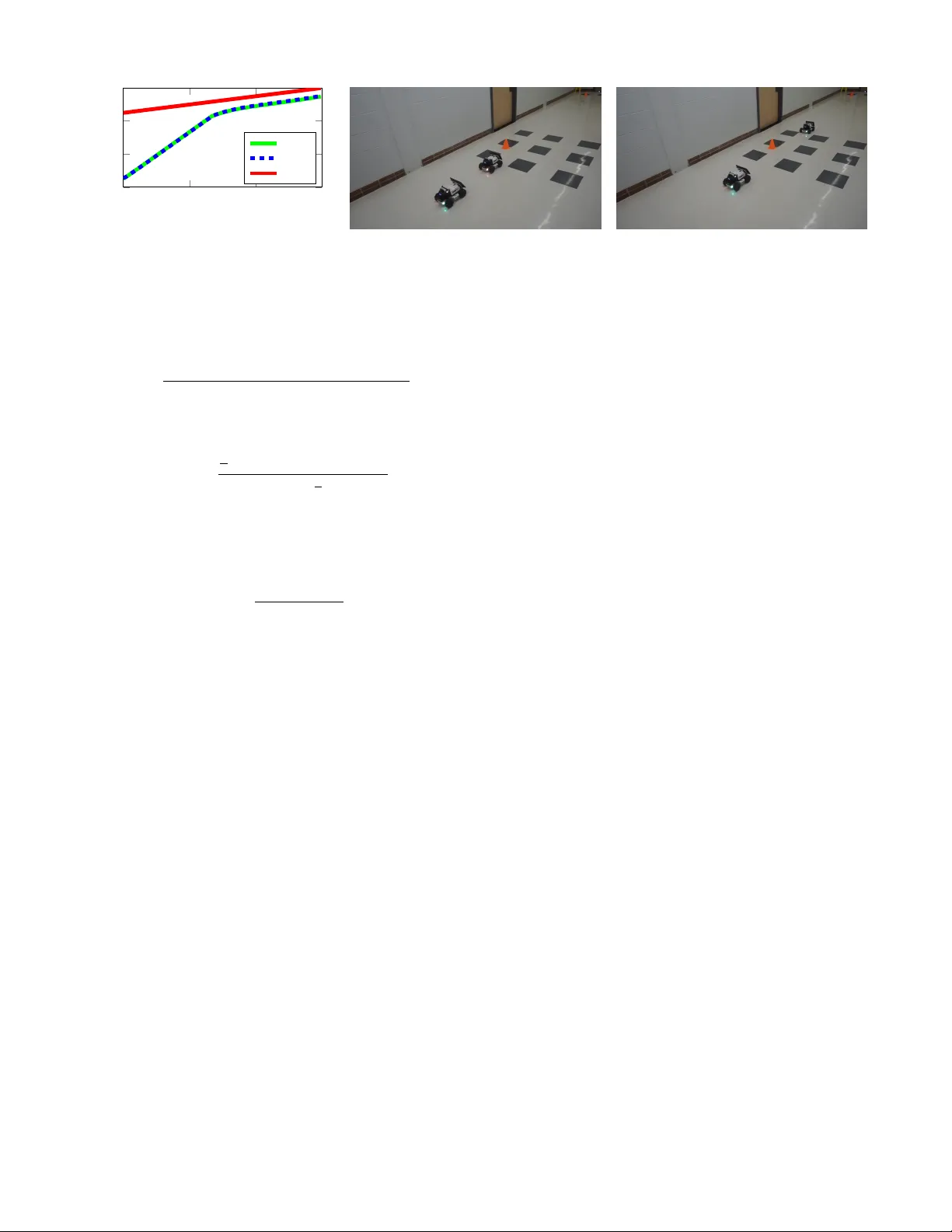
Safety-Constrained Optimal Contr ol f or Unkno wn System Dynamics Panagiotis K ounatidis 1 , Student Member , IEEE , and Andreas A. Malikopoulos 2 , Senior Member , IEEE Abstract — In this paper , we present a framew ork for solving continuous optimal control pr oblems when the true system dynamics are approximated through an imperfect model. W e derive a control strategy by applying Pontryagin’ s Minimum Principle to the model-based Hamiltonian functional, which includes an additional penalty term that captur es the de viation between the model and the true system. W e then derive conditions under which this model-based strategy coincides with the optimal control strategy for the true system under mild convexity assumptions. W e demonstrate the framework on a r eal robotic testbed for the cruise control application with safety distance constraints. I . I N T R O D U C T I O N Optimal control [1], [2] seeks to deriv e a control strategy that minimizes a cost function which encodes desired behav- ior from our system of interest while meeting its ph ysical constraints. In searching of this optimal control strategy , the physical dynamics of the system and any constraints on its state and control inputs must be satisfied. This problem is generally a hard one and typically lacks closed-form analytical solutions except for a fe w classes of systems, for e xample, linear ones with quadratic cost functionals (LQR) [3]. The main theoretical tools to tackle optimal control-the calculus of variations, Pontryagin’ s Minimum Principle (PMP), and dynamic programming-all assume a perfect model of the system dynamics. Adding to the difficulties, in many control applications, e.g., autonomous driving, the system dynamics are often too complex or costly to model precisely . As a result, approximate models are used instead for control synthesis that act as proxies or digital twins for the real system dynamics. Ho we ver , the underlying model mismatch imposes degradation of performance and potential implications on the robust operation of the closed-loop system [4], [5]. This raises the question: when does a contr ol policy derived fr om an appr oximate model r emain optimal for the true system? Addressing this question requires identifying structural properties of optimal control problems that render them insensitiv e to model inaccuracies [6]. A. Related W ork Sev eral research directions aim to circumv ent the need of a model o verall and its entailed suboptimality by directly learn- This research was supported in part by NSF under Grants CNS-2401007, CMMI-2348381, IIS-2415478, and in part by MathW orks. 1 Systems Engineering Program, Cornell University , Ithaca, NY , USA. 2 Andreas A. Malikopoulos is with the Applied Mathematics, Systems Engineering, Mechanical Engineering, Electrical & Computer Engineering, and School of Civil & En vironmental Engineering, Cornell University , Ithaca, NY , USA. Emails: { pk586,amaliko } @cornell.edu . ing the optimal control strategy from data of the real system. Reinforcement learning (RL) methods do so by repeatedly generating full-horizon trajectories of the real system and updating the parameters of a control strategy-policy search [7], [8]- or learn the optimal cost-to-go function-approximate dynamic programming [9]- or do both in an actor -critic struc- ture [10], [11]. Howe ver , RL ’ s episodic nature of learning can often hinder applications on real hardw are and thus require a high-fidelity simulator where the control strategy is trained upon instead, thereby introducing the problem of model mismatch again. On the other hand, adaptive control aims to improv e closed-loop performance by exploring the state space online within a single episode [12]. For example, it has been shown that the Q-function of the LQR problem can be learned online via recursiv e least squares [13]. A key limitation of adaptiv e control frame works is that they often rely on e xplicit model structures and update laws along with persistence of excitation. In a closely related line of work, a theoretical foundation for integrating learning and optimal control in systems with unknown dynamics has been dev eloped [14], [15], and its applicability has been demonstrated in the context of an LQR problem [16]. This framew ork explicitly accounts for model mismatch through penalized, model- based optimal control formulations that capture deviations from the actual system. More recently , it has been shown that optimal control can often be achieved without exact model identification, pro vided that the learning process preserves the structural properties underlying the equi valence between model-based and plant-based decision making [6]. B. Contributions In this paper , we extend the results of [6] to include safety constraints on the optimal control problem that in volve both the state and the control input. For this constrained setup, we deriv e the structural conditions under which the Hamiltonian minimizers of the model-based and plant-based problems coincide, implying equiv alence of the resulting optimal con- trol trajectories despite differences in system dynamics. T o illustrate the equiv alence and v alidate the frame work, we apply it to a real robotic testbed for the cruise control application with safety distance constraints. The code is publicly av ailable at https://github .com/Panos20102k/Multi- Limo-Control . C. Organization The paper is organized as follows. In Section II , we introduce the continuous optimal control problem with safety constraints and unknown dynamics and the penalized model- based approach. In Section III , we formulate the correspond- ing Hamiltonian systems and their optimality conditions. In Section IV , we establish the equi valence results for a general class of Hamiltonian functions as well as those with quadratic control ef fort. In Section V , we apply the framew ork presented for a cruise control e xperiment with real hardware. Finally , in Section VI we provide concluding remarks and directions for future research. I I . P RO B L E M F O R M U L A T I O N W e consider the finite horizon optimal control problem for a continuous dynamical system whose exact dynamics are unknown and is required to satisfy some safety constraints. A. Modeling framework The ev olution of the actual system (plant) is ˙ ˆ x ( t ) = ˆ f ( t, ˆ x ( t ) , u ( t )) , ˆ x (0) = x 0 , (1) and is constrained to satisfy c ( t, ˆ x ( t ) , u ( t )) ≤ 0 , for all t ∈ [0 , T ] , (2) where ˆ x ( t ) ∈ R n , u ( t ) ∈ U ⊂ R m and ˆ f : [0 , T ] × R n × U → R n is an unknown dynamics map which satisfies standard regularity conditions (e.g., Carath ´ eodory conditions) such that for any admissible control u ( · ) ∈ U , the system ( 1 ) admits a unique absolutely continuous solution. The function c : [0 , T ] × R n × U → R is a known constraint map. Remark 1: Considering c to be a scalar function is not restrictiv e, as any l -vector constraint function ( l ≤ m ) can be written compactly in one scalar function through the unit Heaviside step function [1]. W e consider that ˆ x ( t ) is fully observed for all t ∈ [0 , T ] . The model of the actual system that we have access to is giv en by ˙ x ( t ) = f ( t, x ( t ) , u ( t )) , x (0) = x 0 , (3) and the corresponding constraint, c ( t, x ( t ) , u ( t )) ≤ 0 , for all t ∈ [0 , T ] , (4) where x ( t ) ∈ R n and f : [0 , T ] × R n × U → R n is a known dynamics map. Remark 2: The model and the plant share the same initial condition x 0 and are driv en by the same control input u ( · ) . The model state x ( t ) is av ailable at all times. B. Original optimal contr ol pr oblem for the actual system The performance of the actual system is ev aluated through J act = Z T 0 ℓ ( t, ˆ x ( t ) , u ( t )) dt + ϕ ( ˆ x ( T )) , (5) where ℓ : [0 , T ] × R n × U → R is the running cost and ϕ : R n → R the terminal cost. The problem we want to address is given as follows: Problem 1: Minimize J act ov er u ( · ) ∈ U , subject to ( 1 ) and ( 2 ). Howe ver , the plant dynamics ˆ f are unkno wn, so Problem 1 cannot be solved directly . C. Model-based surr ogate pr oblem with penalized cost T o overcome the lack of knowledge of ˆ f , we construct a surrogate optimal control problem based on the kno wn model dynamics ( 3 ). The key idea is to augment the running cost with a penalty term that quantifies the discrepancy between the model state and the observed plant state. T o this end, define J mod = Z T 0 ℓ ( t, x ( t ) , u ( t )) + β ( t ) || x ( t ) − ˆ x ( t ) || 2 dt (6) + ϕ ( x ( T )) , (7) where β : [0 , T ] → R is a gi ven time-v arying weighting function. Then, we consider the following problem. Problem 2: Minimize J mod ov er u ( · ) ∈ U , subject to ( 3 ) and ( 4 ). I I I . H A M I LTO N I A N A NA LY S I S A N D O P T I M A L I T Y C O N D I T I O N S In this section, we deriv e the optimality conditions for the original optimal control problem (Problem 1 ) and the model-based penalized problem (Problem 2 ) through PMP . Throughout our exposition, we consider that the regularity conditions required for the application of PMP are satisfied. W e also suppress the dependence of v ariables on time for clarity of exposition. A. Hamiltonian for the actual system The Hamiltonian functional associated with Problem 1 is ˆ H ( t, ˆ x, u, ˆ λ, ˆ µ ) = ℓ ( t, ˆ x, u ) + ˆ λ T ˆ f ( t, ˆ x, u ) + ˆ µc ( t, ˆ x, u ) , (8) where ˆ λ ∈ R n and ˆ µ ∈ R are the costates and Lagrange multiplier associated with the plant dynamics and constraint, respectiv ely . Based on PMP , if u ∗ ( · ) ∈ U is an optimal control for Problem 1 with corresponding state trajectory ˆ x ∗ ( · ) , then there exists a continuous costate trajectory ˆ λ ∗ ( · ) such that, for almost every t ∈ [0 , T ] , ˙ ˆ x ∗ = ˆ f ( t, ˆ x ∗ , u ) , ˆ x ∗ (0) = x 0 , (9) ˙ ˆ λ ∗ =        − ∇ ˆ x  ℓ ( t, ˆ x ∗ , u ∗ ) + ( ˆ λ ∗ ) T ˆ f ( t, ˆ x ∗ , u ∗ ) + ˆ µ ∗ c ( t, ˆ x ∗ , u ∗ )  , c = 0 , − ∇ ˆ x  ℓ ( t, ˆ x ∗ , u ∗ ) + ( ˆ λ ∗ ) T ˆ f ( t, ˆ x ∗ , u ∗ )  , c < 0 , (10) with terminal condition ˆ λ ∗ ( T ) = ∇ ˆ x ( ϕ ( ˆ x ∗ ( T ))) . Moreov er, the optimal control satisfies the pointwise constrained mini- mization condition u ∗ ∈ arg min u ∈U ˆ H ( t, ˆ x ∗ , u, ˆ λ ∗ , ˆ µ ∗ ) . (11) For the inacti ve safety constraint case, c < 0 , we hav e ˆ µ ∗ = 0 and ( 11 ) determines u ∗ . For c = 0 , ( 2 ) and ( 11 ) together determine u ∗ and ˆ µ ∗ . The Lagrange multiplier ˆ µ ∗ is needed for ( 10 ). Remark 3: If the safety constraints are of the form c ( t, ˆ x ) ≤ 0 , i.e., not an explicit function of u , then we differentiate c with respect to t until its q -th deriv ativ e, c ( q ) ( t, ˆ x, u ) , depends explicitly on u , q ≥ 1 . The optimality conditions are then identical to ( 9 )–( 11 ) with c ( q ) substituted for c and with the addition that for the acti ve constraint case, the follo wing “tangency” conditions must also hold [2], N ( ˆ x, t ) . = [ c ( ˆ x, t ) ˙ c ( ˆ x, t ) . . . c ( q − 1) ( ˆ x, t )] T = 0 . (12) B. Hamiltonian for the model-based penalized problem The Hamiltonian functional associated with Problem 2 is H ( t, x, ˆ x, u, λ, µ ) = ℓ ( t, x, u ) + λ T f ( t, x, u ) + β || x − ˆ x || 2 + µc ( t, x, u ) , (13) where λ ∈ R n and µ ∈ R are the costates and Lagrange mul- tiplier associated with the model dynamics and constraint, respectiv ely . If u ◦ ( · ) ∈ U is an optimal control for Problem 2 with corresponding state trajectory x ◦ ( · ) , then there exists a continuous costate trajectory λ ◦ ( · ) such that, for almost e very t ∈ [0 , T ] , ˙ x ◦ = f ( t, x ◦ , u ) , x ◦ (0) = x 0 , (14) ˙ λ ◦ =            − ∇ x  ℓ ( t, x ◦ , u ◦ ) + ( λ ◦ ) T f ( t, x ◦ , u ◦ ) + β || x ◦ − ˆ x || 2 + µ ◦ c ( t, x ◦ , u ◦ )  , c = 0 , − ∇ x  ℓ ( t, x ◦ , u ◦ ) + ( λ ◦ ) T f ( t, x ◦ , u ◦ ) + β || x ◦ − ˆ x || 2  , c < 0 , (15) with terminal condition λ ◦ ( T ) = ∇ x ( ϕ ( x ◦ ( T ))) . Moreov er, the optimal control satisfies the pointwise constrained mini- mization condition u ◦ ∈ arg min u ∈U H ( t, x ◦ , ˆ x, u, λ ◦ , µ ◦ ) . (16) If the constraints are not an explicit function of u , then we substitute c ( q ) ( t, x, u ) for c in ( 15 ) and additionally require for the active constraint case that N ( x, t ) . = [ c ( x, t ) ˙ c ( x, t ) . . . c ( q − 1) ( x, t )] T = 0 . (17) C. Constrained Hamiltonian minimization. Existence and uniqueness Next, we provide conditions under which the pointwise Hamiltonian minimization problems that arise in ( 11 ) and ( 16 ) admit minimizers. Assumption 1. The admissible control set U ⊂ R m is nonempty , closed, and conv ex (not necessarily bounded). Assumption 2. F or almost ev ery t ∈ [0 , T ] and for all relev ant ( ˆ x, ˆ λ, ˆ µ ) and ( x, ˆ x, λ, µ ) , the maps u 7→ ˆ H ( t, ˆ x, u, ˆ λ, ˆ µ ) and u 7→ H ( t, x, ˆ x, u, λ, µ ) , are proper , lo wer semicontinuous, and con vex on U . More- ov er, they are coerciv e on U , i.e., ∥ u ∥ → ∞ , u ∈ U = ⇒ ˆ H ( t, ˆ x, u, ˆ λ, ˆ µ ) → + ∞ and H ( t, x, ˆ x, u, λ, µ ) → + ∞ . Theorem 1. Suppose Assumptions 1 – 2 hold. Then, for al- most every t ∈ [0 , T ] , the sets of minimizers arg min u ∈U ˆ H ( t, ˆ x, u, ˆ λ, ˆ µ ) and arg min u ∈U H ( t, x, ˆ x, u, λ, µ ) , ar e nonempty , closed, and con vex. If, in addition, for almost every t the Hamiltonians are strictly con vex in u on U (e.g ., α -str ongly con vex), then these minimizers ar e unique almost everywher e. Pr oof: See [6]. I V . E Q U I V A L E N C E R E S U LT S All equi valence results in this section are pointwise in time and rely on the structure of the instantaneous Hamiltonian minimization problems induced by the two optimal control formulations. W e provide two complementary equiv alences results. The first is stated in a con ve x-analysis form (subdif- ferentials and normal cones) and accommodates nonsmooth costs, unbounded control sets, and nonlinear dynamics, pro- vided the pointwise Hamiltonian minimization problems are con vex. The second result specializes in a commonly used structural setting (quadratic control effort and mild growth conditions), which yields simple, v erifiable conditions for existence, uniqueness, and equiv alence. A. Conve x analysis preliminaries Let U ⊂ R m be nonempty , closed, and con vex. The normal cone to U at u ∈ U is defined by N U ( u ) := { η ∈ R m : ⟨ η , v − u ⟩ ≤ 0 , ∀ v ∈ U } . For a proper , lower semicontinuous, con vex function ψ : R m → R ∪ { + ∞} , the con vex subdifferential at u is denoted by ∂ ψ ( u ) . W e will use the standard fact that u ∗ ∈ arg min u ∈U ψ ( u ) if and only if 0 ∈ ∂ ψ ( u ∗ ) + N U ( u ∗ ) . Remark 4: Under Assumption 1 and con ve xity of u 7→ H ( t, · ) , u ∗ minimizes H ( t, · ) over U if and only if 0 ∈ ∂ u H ( t, u ∗ ) + N U ( u ∗ ) , where ∂ u denotes the conv ex subdifferential and N U is the normal cone to U . If H is differentiable in u , this reduces to the variational inequality ⟨∇ u H ( t, u ∗ ) , v − u ∗ ⟩ ≥ 0 , ∀ v ∈ U . B. General equivalence r esults Theorem 2. Suppose Assumptions 1 – 2 hold and let C := { u ∈ U : c ( · , u ) ≤ 0 } , wher e the safety constraint as a function of u , c ( · , u ) , is pr oper , lower semicontinuous, and con vex, and C is nonempty . F ix any t ∈ [0 , T ] for whic h the pointwise constrained Hamiltonian minimization pr oblems are well posed, and define Ψ act ( u ; t ) := ˆ H ( t, ˆ x, u, ˆ λ, ˆ µ ) , (18) Ψ mod ( u ; t ) := H ( t, x, ˆ x, u, λ, µ ) , (19) for u ∈ C . Assume that there exists ¯ u ∈ C such that ∂ u ˆ H ( t, ˆ x, ¯ u, ˆ λ, ˆ µ ) = ∂ u H ( t, x, ˆ x, ¯ u, λ, µ ) . (20) Then 0 ∈ ∂ u ˆ H ( t, ˆ x, ¯ u, ˆ λ, ˆ µ ) + N C ( ¯ u ) ⇐ ⇒ 0 ∈ ∂ u H ( t, x, ˆ x, ¯ u, λ, µ ) + N C ( ¯ u ) . (21) Consequently , if either one of the inclusions in ( 21 ) holds, then ¯ u is a minimizer for both pointwise constrained Hamil- tonian pr oblems, that is, ¯ u ∈ arg min u ∈C ˆ H ( t, ˆ x, u, ˆ λ, ˆ µ ) ∩ arg min u ∈C H ( t, x, ˆ x, u, λ, µ ) . (22) If, in addition, each Hamiltonian is strictly con vex in u on C , then each argmin is a singleton; hence, the two minimizers ar e unique and coincide. Pr oof: Since U is closed and con ve x and c ( · , u ) is con vex, lo wer semicontinuous, and proper , the feasible set C := { u ∈ U : c ( · , u ) ≤ 0 } , is closed and con vex. By assumption, it is nonempty . By Assumptions 1 – 2 , both Ψ act ( · ; t ) and Ψ mod ( · ; t ) are proper , lower semicontinuous, and con vex on C , and the corresponding constrained minimization problems are well posed. For an y proper , lower semicontinuous, con vex function Ψ : U → R ∪ { + ∞} and any nonempty closed con vex set C , the standard first-order condition for conv ex minimization over C is ¯ u ∈ arg min u ∈C Ψ( u ) ⇐ ⇒ 0 ∈ ∂ Ψ( ¯ u ) + N C ( ¯ u ) . (23) Applying ( 23 ) to Ψ act ( · ; t ) and Ψ mod ( · ; t ) gi ves ¯ u ∈ arg min u ∈C ˆ H ( t, ˆ x, u, ˆ λ, ˆ µ ) ⇐ ⇒ 0 ∈ ∂ u ˆ H ( t, ˆ x, ¯ u, ˆ λ, ˆ µ ) + N C ( ¯ u ) , (24) ¯ u ∈ arg min u ∈C H ( t, x, ˆ x, u, λ, µ ) ⇐ ⇒ 0 ∈ ∂ u H ( t, x, ˆ x, ¯ u, λ, µ ) + N C ( ¯ u ) . (25) Now ( 20 ) implies that ∂ u ˆ H ( t, ˆ x, ¯ u, ˆ λ, ˆ µ ) + N C ( ¯ u ) = ∂ u H ( t, x, ˆ x, ¯ u, λ, µ ) + N C ( ¯ u ) . Hence the two inclusions in ( 21 ) are equiv alent. Using ( 24 )–( 25 ), either inclusion implies that ¯ u minimizes both Hamiltonians over C , which proves ( 22 ). If each Hamiltonian is strictly con vex in u on C , then each constrained minimization problem admits at most one minimizer . Since ( 22 ) shows that the two argmin sets contain the same element ¯ u , both ar gmin sets are singletons and equal to { ¯ u } . Therefore, the minimizers are unique and coincide. C. Specialization to quadratic contr ol effort While Theorem 2 provides a general equiv alence result under con ve xity , its hypotheses may be abstract to verify directly . Next, we specialize in quadratic control ef fort under which the equiv alence becomes explicit and easily verifiable. Assumption 3. The admissible control set U ⊂ R m is nonempty , closed, and con ve x (possibly unbounded). The running cost has the form ℓ ( t, z , u ) = ℓ 0 ( t, z ) + 1 2 u ⊤ R ( t ) u, (26) where ℓ 0 ( t, · ) is continuous in z and R ( t ) ∈ R m × m satisfies R ( t ) ⪰ r min I , for some r min > 0 and all t ∈ [0 , T ] . Assumption 3 guarantees uniform strong con ve xity of the Hamiltonian with respect to the control input, ensuring the existence and uniqueness of the pointwise optimal control and well-posedness of the minimization problem ov er the entire time horizon. Intuiti vely , this condition ensures that control effort is penalized in ev ery direction at all times, so the optimal control cannot be flat, ill-defined, or sensitiv e to small perturbations. Assumption 4. F or almost e very t and all rele vant ( x, ˆ x, λ, ˆ λ ) , the maps u 7→ λ ⊤ f ( t, x, u ) , u 7→ ˆ λ ⊤ ˆ f ( t, ˆ x, u ) , u 7→ µc ( t, x, u ) , u 7→ ˆ µc ( t, ˆ x, u ) , are con vex on U , and satisfy a linear growth bound, i.e., there exist locally bounded functions c f ( t, x ) , c ˆ f ( t, ˆ x ) , c c ( t, ˆ x ) , c c ( t, x ) ≥ 0 such that for all u ∈ U , | λ ⊤ f ( t, x, u ) | ≤ c f ( t, x )(1 + ∥ u ∥ ) , | ˆ λ ⊤ ˆ f ( t, ˆ x, u ) | ≤ c ˆ f ( t, ˆ x )(1 + ∥ u ∥ ) , | ˆ µc ( t, ˆ x, u ) | ≤ c c ( t, ˆ x )(1 + || u || ) , | µ ( t, x, u ) | ≤ c c ( t, x )(1 + || u || ) . Assumption 4 imposes a linear-gro wth condition on the control-dependent terms of the Hamiltonian, ensuring co- ercivity and preventing unbounded descent ev en when the admissible control set is unbounded. In simple terms, this condition guarantees that no term in the dynamics or cost can ov erpower the quadratic control penalty , so the optimization does not “prefer” arbitrarily large control actions. Lemma 1. Under Assumptions 3 – 4 , for almost every t the pointwise minimization problems arg min u ∈U ˆ H ( t, ˆ x, u, ˆ λ, ˆ µ ) , arg min u ∈U H ( t, x, ˆ x, u, λ, µ ) , admit unique minimizers. Pr oof: Fix t ∈ [0 , T ] such that Assumptions 3 – 4 hold (this is the case for almost e very t ). W e prove the claim for the model-based Hamiltonian. The proof for the plant Hamiltonian is identical. For fixed ( t, x, ˆ x, λ ) , we define the function Ψ( u ) := H ( t, x, ˆ x, u, λ, µ ) = ℓ 0 ( t, x ) + 1 2 u ⊤ R ( t ) u + β ( t ) ∥ x − ˆ x ∥ 2 + λ ⊤ f ( t, x, u ) + µc ( t, x, u ) . (27) By Assumption 4 , the maps u 7→ λ ⊤ f ( t, x, u ) and u 7→ µc ( t, x, u ) are conv ex on U . Therefore Ψ is con vex on U . Moreov er, since R ( t ) ⪰ r min I , the quadratic term is r min - strongly con ve x on U , hence Ψ is strongly con vex on U as the sum of a strongly conv ex function and two con ve x functions. Let r max ( t ) := ∥ R ( t ) ∥ and note that 1 2 u ⊤ R ( t ) u ≥ r min 2 ∥ u ∥ 2 , ∀ u ∈ U . By Assumption 4 , Ψ( u ) ≥  ℓ 0 ( t, x ) + β ( t ) ∥ x − ˆ x ∥ 2  + r min 2 ∥ u ∥ 2 − ( c f ( t, x ) + c c ( t, x ))(1 + ∥ u ∥ ) . The right-hand side is a quadratic function of ∥ u ∥ with positiv e leading coefficient r min 2 ; therefore, ∥ u ∥ → ∞ , u ∈ U = ⇒ Ψ( u ) → + ∞ . Namely , Ψ is coercive on U . Let m ⋆ := inf u ∈U Ψ( u ) and let { u k } ⊂ U be a minimizing sequence with Ψ( u k ) ↓ m ⋆ . Coercivity implies that { u k } is bounded. Otherwise ∥ u k ∥ → ∞ along a subsequence would force Ψ( u k ) → + ∞ , contradicting Ψ( u k ) ↓ m ⋆ < + ∞ . Since { u k } is bounded, there exists a subsequence (not relabeled) and ¯ u ∈ R m such that u k → ¯ u . Because U is closed, ¯ u ∈ U . Finally , Ψ is conv ex (hence continuous on the relativ e interior of U ) and, under the present assumptions, lower semicontinuous on U ; thus Ψ( ¯ u ) ≤ lim inf k →∞ Ψ( u k ) = m ⋆ , which yields Ψ( ¯ u ) = m ⋆ . Therefore, ¯ u is a minimizer and the argmin set is nonempty . Because Ψ is strongly conv ex on U , it admits at most one minimizer on U . Indeed, if u 1  = u 2 were both minimizers, then for any θ ∈ (0 , 1) strong con ve xity would imply Ψ( θ u 1 + (1 − θ ) u 2 ) < θ Ψ( u 1 ) + (1 − θ )Ψ( u 2 ) = m ⋆ , a contradiction. Hence, the minimizer is unique. Theorem 3. Suppose Assumptions 3 – 4 hold. Let ( ˆ x ∗ , ˆ λ ∗ , ˆ µ ∗ , u ∗ ) satisfy the PMP conditions for the plant pr oblem (Pr oblem 1 ), and let ( x ◦ , λ ◦ , µ ◦ , u ◦ ) satisfy the PMP conditions for the model-based penalized problem (Pr oblem 2 ). Suppose that, for almost every t ∈ [0 , T ] , ∇ u h ℓ ( t, ˆ x ∗ , u ) + ˆ λ ∗⊤ ˆ f ( t, ˆ x ∗ , u ) + ˆ µ ∗ c ( t, ˆ x ∗ , u ) i = ∇ u  ℓ ( t, x ◦ , u ) + λ ◦⊤ f ( t, x ◦ , u ) + µ ◦ c ( t, x ◦ , u )  , (28) at u = u ◦ , and that the state alignment holds: x ◦ ( t ) = ˆ x ∗ ( t ) for a.e. t ∈ [0 , T ] . (29) Then u ◦ ( t ) = u ∗ ( t ) , for a.e. t ∈ [0 , T ] . A sufficient set of verifiable conditions implying ( 28 ) is: ∇ u ˆ f ( t, ˆ x ∗ ( t ) , u ) = ∇ u f ( t, x ◦ ( t ) , u ) for all u ∈ U , a.e. t, λ ◦ ( t ) = ˆ λ ∗ ( t ) a.e. , µ ◦ ( t ) = ˆ µ ∗ ( t ) a.e. (30) Pr oof: W e prove that u ◦ ( t ) = u ∗ ( t ) for almost e very t ∈ [0 , T ] . The proof is pointwise in time and relies on (i) uniqueness of the pointwise Hamiltonian minimizers (Lemma 1) and (ii) the switching-gradient matching con- dition ( 28 ). By Lemma 1, under Assumptions ( 3 )–( 4 ), for almost ev ery t ∈ [0 , T ] , the pointwise minimization problems arg min u ∈U ˆ H  t, ˆ x ∗ ( t ) , u, ˆ λ ∗ ( t ) , ˆ µ ∗ ( t )  and arg min u ∈U H  t, x ◦ ( t ) , ˆ x ∗ ( t ) , u, λ ◦ ( t ) , µ ◦ ( t )  , admit unique minimizers. W e fix such a time t and suppress the explicit dependence on t in the notation. W e define the pointwise objective functions Ψ act ( u ) := ˆ H ( ˆ x ∗ , u, ˆ λ ∗ , ˆ µ ∗ ) , (31) Ψ mod ( u ) := H ( x ◦ , ˆ x ∗ , u, λ ◦ , µ ◦ ) . (32) Then, by definition of the PMP minimization conditions, u ∗ = arg min u ∈U Ψ act ( u ) , u ◦ = arg min u ∈U Ψ mod ( u ) . (33) Under Assumptions ( 3 )–( 4 ), both Ψ act and Ψ mod are con- ve x and (by the standing smoothness conditions in the PMP setup) differentiable in u . Therefore, the unique minimizer u ◦ of Ψ mod satisfies the variational inequality ⟨∇ u Ψ mod ( u ◦ ) , v − u ◦ ⟩ ≥ 0 , ∀ v ∈ U . (34) Similarly , u ∗ is characterized by the corresponding v aria- tional inequality for Ψ act : ⟨∇ u Ψ act ( u ∗ ) , v − u ∗ ⟩ ≥ 0 , ∀ v ∈ U . (35) By the definitions of the Hamiltonians, ∇ u Ψ act ( u ) = ∇ u h ℓ  t, ˆ x ∗ , u  + ˆ λ ∗⊤ ˆ f  t, ˆ x ∗ , u  + ˆ µ ∗ c ( t, ˆ x ∗ , u ) i , (36) ∇ u Ψ mod ( u ) = ∇ u h ℓ  t, x ◦ , u  + λ ◦⊤ f  t, x ◦ , u  + µ ◦ c ( t, x ◦ , u ) i , (37) where we have used the penalty term β ∥ x ◦ − ˆ x ∗ ∥ 2 does not depend explicitly on u at fixed ( t, x ◦ , ˆ x ∗ ) , and hence does not contribute to ∇ u Ψ mod . From the hypothesis, ∇ u Ψ act ( u )   u = u ◦ = ∇ u Ψ mod ( u )   u = u ◦ . (38) (Condition ( 29 ) ensures that the state arguments appearing in the two gradients are e valuated consistently along the relev ant trajectory .) Substituting ( 38 ) into the variational inequality ( 34 ) yields ⟨∇ u Ψ act ( u ◦ ) , v − u ◦ ⟩ ≥ 0 , ∀ v ∈ U . (39) Since Ψ act is conv ex and dif ferentiable on the closed con vex set U , the v ariational inequality ( 39 ) is equiv alent to the statement that u ◦ is a minimizer of Ψ act ov er U , i.e., u ◦ ∈ arg min u ∈U Ψ act ( u ) . But by Lemma 1, this ar gmin set is the singleton { u ∗ } . Therefore, u ◦ = u ∗ . The argument above holds for every t at which the pointwise minimizers are unique and the matching condition ( 28 ) holds. From the hypothesis, ( 28 ) and ( 29 ) hold for almost e very t , and by Lemma 1, uniqueness holds for almost every t . Hence, u ◦ ( t ) = u ∗ ( t ) for a.e. t ∈ [0 , T ] , which completes the proof. Finally , the sufficient conditions ( 30 ) imply ( 28 ) by direct substitution into ( 36 )–( 37 ), since equality of ∇ u ˆ f and ∇ u f (together with λ ◦ = ˆ λ ∗ , µ ◦ = ˆ µ ∗ and x ◦ = ˆ x ∗ ) yields equality of the Hamiltonian gradients at u = u ◦ ( t ) . V . C R U I S E C O N T RO L E X A M P L E In this section, we apply our framework to a cruise control application using the LIMO ROS 2 robots [17]. Specifically , we consider an ego LIMO that we control, and another LIMO in the front that we do not control. A. Plant and model dynamics Let ˆ x . = [ ˆ p ˆ v ] T ∈ R 2 denote the state of the plant consisting of the position and velocity of the ego LIMO . The admissible control space is the one-dimensional simplex on the real line defined by the minimum and maximum admissible control input, i.e., U . = [ u min , u max ] . The plant is assumed to follow double integrator dynamics with first- order actuation lag, ˙ ˆ x =  0 1 0 − 1 ˆ τ  ˆ x +  0 ˆ k ˆ τ  u, ˆ x (0) = x 0 , (40) with actuation gain ˆ k > 0 and delay time constant ˆ τ > 0 , and is constrained to satisfy c ( ˆ x ) . = δ − ξ ( p f − ˆ p ) ≤ 0 , for all t ∈ [0 , T ] , (41) where δ > 0 is the safety distance from the front car, p f ∈ R the position of the front car and ξ > 0 the reaction time coefficient. Now , let x . = [ p v ] T ∈ R 2 denote the state of the model that we have access to, with dynamics given by ˙ x =  0 1 0 − 1 τ  x +  0 k τ  u, x (0) = x 0 , (42) and the corresponding constraint c ( x ) . = δ − ξ ( p f − p ) ≤ 0 , for all t ∈ [0 , T ] . (43) B. Cost function and constraints The performance of the plant is ev aluated through J act = Z T 0 [ q ( ˆ v − v ref ) 2 + r ˆ a 2 ] dt + h [ ˆ v ( T ) − v ref ] 2 , (44) where q , r, h > 0 , which penalizes deviation from the reference velocity v ref and excessi ve acceleration ˆ a . = ˆ k u − ˆ v ˆ τ = ˙ ˆ v. (45) The cost functional that the model-based surrogate problem with penalized cost considers is J mod = Z T 0 [ q ( v − v ref ) 2 + r a 2 ] dt + h [ v ( T ) − v ref ] 2 . (46) C. Hamiltonian minimization and contr ol laws W e no w deriv e the control strategy of the model-based surrogate problem. The Hamiltonian is H = q ( v − v ref ) 2 + r a 2 + λ 1 v + λ 2 a + µc ( x, u ) + β 1 ( p − ˆ p ) 2 + β 2 ( v − ˆ v ) 2 , (47) where c ( x, u ) is the second time deriv ative of ( 43 ). Impor- tantly , the penalty terms do not depend on u and therefore do not affect the pointwise minimization of the Hamiltonian with respect to the control input. The time that the safety constraint becomes active for the first time is t s . = { arg min t ∈ [0 ,T ] t, c ( x ) = 0 } . (48) Case 1: Inactive safety constraint For t ∈ [0 , t s ] , based on the optimality conditions ( 14 )– ( 16 ), the optimal unconstrained state, costate, and control input trajectories satisfy the follo wing system of differential equations. λ 2 = − 2 r a, (49) ˙ λ 1 = − 2 β 1 ( p − ˆ p ) , λ 1 ( T ) = 0 , (50) ˙ λ 2 = − 2 q ( v − v ref ) − λ 1 + 2 r a + λ 2 τ − 2 β 2 ( v − ˆ v ) , (51) with boundary condition λ 2 ( T ) = 2 h ( v ( T ) − v ref ) and ( 42 ). Using the state alignment condition of Theorem 3 , ( 50 ) yields λ 1 = 0 . Using this, ( 49 ) and the state alignment condition, ( 51 ) becomes ˙ λ 2 = − 2 q ( v − v ref ) . (52) By dif ferentiating now ( 49 ) with respect to time and using ( 52 ) yields ¨ v = q r ( v − v ref ) , (53) which is a second-order ordinary differential equation of the form ¨ w = ω 2 w , (54) with w . = v − v ref and ω . = p q r . The analytical solution to ( 54 ) for initial condition w 0 . = v (0) − v ref yields the 0 5 10 15 2 4 6 8 T ime Position p opt p mb p f (a) Position over time of front and ego LIMO (b) t = 6 s (c) t = 1 s Fig. 1: Position trajectories (Figure 1a ) and snapshots during one run (Figures 1b and 1c ). closed-form optimal unconstrained control input and velocity trajectory , u ∗ ( t ) = v ∗ ( t ) + τ ω [ w 0 sinh( ω t ) + B cosh( ω t )] k , (55) v ∗ ( t ) = v ref + w 0 cosh( ω t ) + B sinh( ω t ) , (56) for t ∈ [0 , t s ] , where B = − ω 0 h r cosh( ω T ) + ω sinh( ω T ) ω cosh( ω T ) + h r sinh( ω T ) . (57) Case 2: Active safety constraint For t ∈ [ t s , T ] , the active constraint equation c ( x, u ) = 0 along with the tangenc y conditions ( 17 ) yield the optimal constrained control input trajectory , u ∗ ( t ) = ˙ p f ( t ) + τ ¨ p f ( t ) k , (58) for t ∈ [ t s , T ] . In this case, the optimal strategy is to copy the velocity and acceleration profile of the LIMO car in front, and thereby ”ride” the constraint. By considering now the admissible control space, the final PMP control strategy of the model-based surrogate problem is the projection of ( 55 ) and ( 58 ) to the one-dimensional simplex line, i.e., u mb ( t ) = Π [ u min , u max ] [ u ∗ ( t )] , t ∈ [0 , T ] . (59) Now , the Hamiltonian of the original optimal control problem is H = q ( ˆ v − v ref ) 2 + r ˆ a 2 + ˆ λ 1 ˆ v + ˆ λ 2 ˆ a + ˆ µc ( ˆ x, u ) . (60) Similarly , by applying the optimality conditions ( 9 )–( 12 ), the final PMP control strate gy of the original optimal control problem is u opt ( t ) = Π [ u min , u max ] [ u ∗ ( t )] , t ∈ [0 , T ] . (61) where u ∗ ( t ) is given by ( 55 ) and ( 58 ) b ut with the real parameters ˆ τ and ˆ k substituted in these expressions instead of τ and k respectively . Due to this model mismatch, the resulting control strategies differ . Howe ver , the penalty terms in ( 47 ) shape the state and costate e volution of the model-based problem without altering the structure of the Hamiltonian minimization with respect to u . As a result, whenev er the projected minimizers, u mb and u opt , coincide, the optimal control trajectories deriv ed from the model and the plant are identical, as illustrated in the next section. D. Experimental r esults In this section, we present the experimental results of the cruise control application on the LIMO robots, which illus- trate the equiv alence between the optimal control strategies deriv ed in the previous section. The initial state of the ego LIMO (that we control) is x 0 = [0 . 0 0 . 5] T . The desired reference velocity is v ref = 0 . 6 m / s . The dynamics of the ego LIMO are giv en by ( 40 ) with ˆ τ = 0 . 1 and ˆ k = 1 . 4 . The model-based controller, howe ver , assumes τ = 0 . 3 and k = 1 . 2 , hence the model- mismatch. The front LIMO car cruises at a constant speed of 0 . 1 m / s starting from p f = 4 . 0 m . The constraint parameters are δ = 1 m , ξ = 1 while the admissible control set is U = [0 . 1 0 . 4] . The cost parameters are q = h = 1 and r = 0 . 5 . The zero order hold sampling time is selected to 0 . 1 s for a control horizon of T = 15 s . The framew ork is implemented in the R OS 2 system [18]. The main controller node implements the model-based pe- nalized control strategy ( 59 ) and the original optimal control strategy ( 61 ), depending on the desired mode of operation. T o implement these strategies, real-time state feedback of the ego LIMO is required as well as an estimate of the front LIMO ’ s position and velocity . For the former , an extended Kalman filter is utilized from the robot localization package [19]. T o achie ve the latter , in practice, real A CC systems lev erage mainly radar measurements. Howe ver , since the LIMO robots are not equipped with this type of sensor, we implement direct communication of the front LIMO ’ s position and velocity to the controller of the ego LIMO . The code, along with more details on the implementation, is publicly av ailable at https://github .com/Panos20102k/Multi- Limo-Control . W e conduct two runs of the cruise control exam- ple, one for the model-based penalized control and one for the original optimal control, and compare the results. The video of these runs is av ailable at https://www .youtube.com/watch?v=pMSZKlU5O44 . Fig- ure 1 depicts the position trajectories of the LIMO cars in both runs, as well as specific snapshots during one run. p mb and p opt are the position trajectories of the ego LIMO as a result of the model-based control strategy ( 59 ) and the original optimal control strategy ( 61 ), respectively . Figure 2 depicts the control input trajectories generated by ( 59 ) and ( 61 ). These figures illustrate that, despite model-mismatch, 0 2 4 6 8 10 12 14 0 0 . 2 0 . 4 T ime Control Input u opt u mb Fig. 2: Equivalence of control inputs the model-based penalized control strategy can recover the optimal control strategy . This is because the equiv alence of optimal control trajectories follows from the equiv alence of the constrained Hamiltonian minimizers, not from equality of the dynamics. Although the gradients of the plant and model Hamiltonians are different (as reflected in the dif ferent unconstrained minimizers), the admissible control constraints u ∈ U dominate the pointwise minimization. From a theo- retical perspectiv e, the figures highlight that ∇ u ˆ H  = ∇ u H while arg min u ∈U ˆ H = arg min u ∈U H . which is precisely the mechanism underlying the equiv alence results of Section IV . V I . C O N C L U D I N G R E M A R K S In this paper , we studied the finite-horizon continuous optimal control problem with safety constraints and un- known plant dynamics. An approximate model is lev eraged to synthesize a penalized model-based control strategy . W e analyzed the associated Hamiltonian system and established structural conditions under which the constrained Hamilto- nian minimizer of the model-based problem coincides with the minimizer of the original plant problem. W e demon- strated this equiv alence on real hardware experiments of a cruise control application with rear-end safety constraints. A key insight of this framework is that the penalty term capturing model–plant mismatch influences the state and costate ev olution, but does not explicitly enter into the pointwise minimization of the Hamiltonian with respect to the control input. This observation allows us to decouple questions of the model accuracy from control optimality and provides a principled explanation for why approximate models and digital twins can successfully generate optimal control strategies in practice. The results of this paper suggest a shift in perspective for learning-based control. Rather than focusing on exact system identification, learning ef forts can be directed tow ard preserving the structural properties that determine Hamil- tonian minimization. Ongoing work explores implementing this analysis in stochastic systems. R E F E R E N C E S [1] D. Kirk, Optimal Control Theory: An Introduction . Dov er Publica- tions, 2004. [2] A. E. Bryson and Y .-C. Ho, Applied Optimal Control: Optimization, Estimation, and Contr ol . W ashington, DC: Hemisphere Publishing Corporation, 1975. [3] D. P . Bertsekas, Dynamic Pr ogramming and Optimal Contr ol , 4th ed. Athena Scientific, 2017. [4] R. E. Skelton, “Model error concepts in control design, ” International Journal of Control , vol. 49, no. 5, pp. 1725–1753, 1989. [5] S. Sagmeister, P . Kounatidis, S. Goblirsch, and M. Lienkamp, “ Analyz- ing the impact of simulation fidelity on the e valuation of autonomous driving motion control, ” in 2024 IEEE Intelligent V ehicles Symposium (IV) , 2024, pp. 230–237. [6] A. A. Malikopoulos, “When an approximate model suffices for optimal control, ” 2026 (in review), arXiv preprint [7] R. S. Sutton, D. McAllester , S. Singh, and Y . Mansour, “Policy gradi- ent methods for reinforcement learning with function approximation, ” in Advances in Neural Information Pr ocessing Systems , S. Solla, T . Leen, and K. M ¨ uller , Eds., vol. 12. MIT Press, 1999. [8] B. Recht, “ A tour of reinforcement learning: The vie w from contin- uous control, ” Annual Re view of Contr ol, Robotics, and A utonomous Systems , vol. 2, pp. 253–279, May . 2019. [9] D. P . Bertsekas and J. N. Tsitsiklis, Neur o-Dynamic Pro gramming . Athena Scientific, 1996. [10] K. G. V amvoudakis and F . L. Lewis, “Online actor-critic algorithm to solve the continuous-time infinite horizon optimal control problem, ” Automatica , vol. 46, no. 5, pp. 878–888, 2010. [11] B. Kiumarsi, K. G. V amvoudakis, H. Modares, and F . L. Lewis, “Opti- mal and autonomous control using reinforcement learning: A surve y , ” IEEE T ransactions on Neural Networks and Learning Systems , vol. 29, no. 6, pp. 2042–2062, 2018. [12] P . Ioannou and B. Fidan, Adaptive Contr ol T utorial . Philadelphia, P A: Society for Industrial and Applied Mathematics, 2006. [13] S. Bradtke, B. Ydstie, and A. Barto, “ Adaptiv e linear quadratic control using policy iteration, ” in Proceedings of 1994 American Control Confer ence - ACC ’94 , vol. 3, 1994, pp. 3475–3479 vol.3. [14] A. A. Malikopoulos, “Separation of learning and control for cyber - physical systems, ” Automatica , vol. 151, no. 110912, 2023. [15] ——, “Combining learning and control in linear systems, ” European Journal of Control , vol. 80, no. Part A, p. 101043, 2024. [16] P . K ounatidis and A. A. Malikopoulos, “Combined learning and control: A ne w paradigm for optimal control with unkno wn dynamics, ” in 65th American Contr ol Confer ence (ACC) , 2025, to appear. [17] Agilex Robotics. [18] S. Macenski, T . Foote, B. Gerke y , C. Lalancette, and W . W oodall, “Robot Operating System 2: Design, architecture, and uses in the wild, ” Science Robotics , vol. 7, no. 66, p. eabm6074, 2022. [19] T . Moore and D. Stouch, “ A generalized extended kalman filter implementation for the robot operating system, ” in Proceedings of the 13th International Conference on Intelligent A utonomous Systems (IAS-13) . Springer, 2014, pp. 335–348.