Energy Score-Guided Neural Gaussian Mixture Model for Predictive Uncertainty Quantification

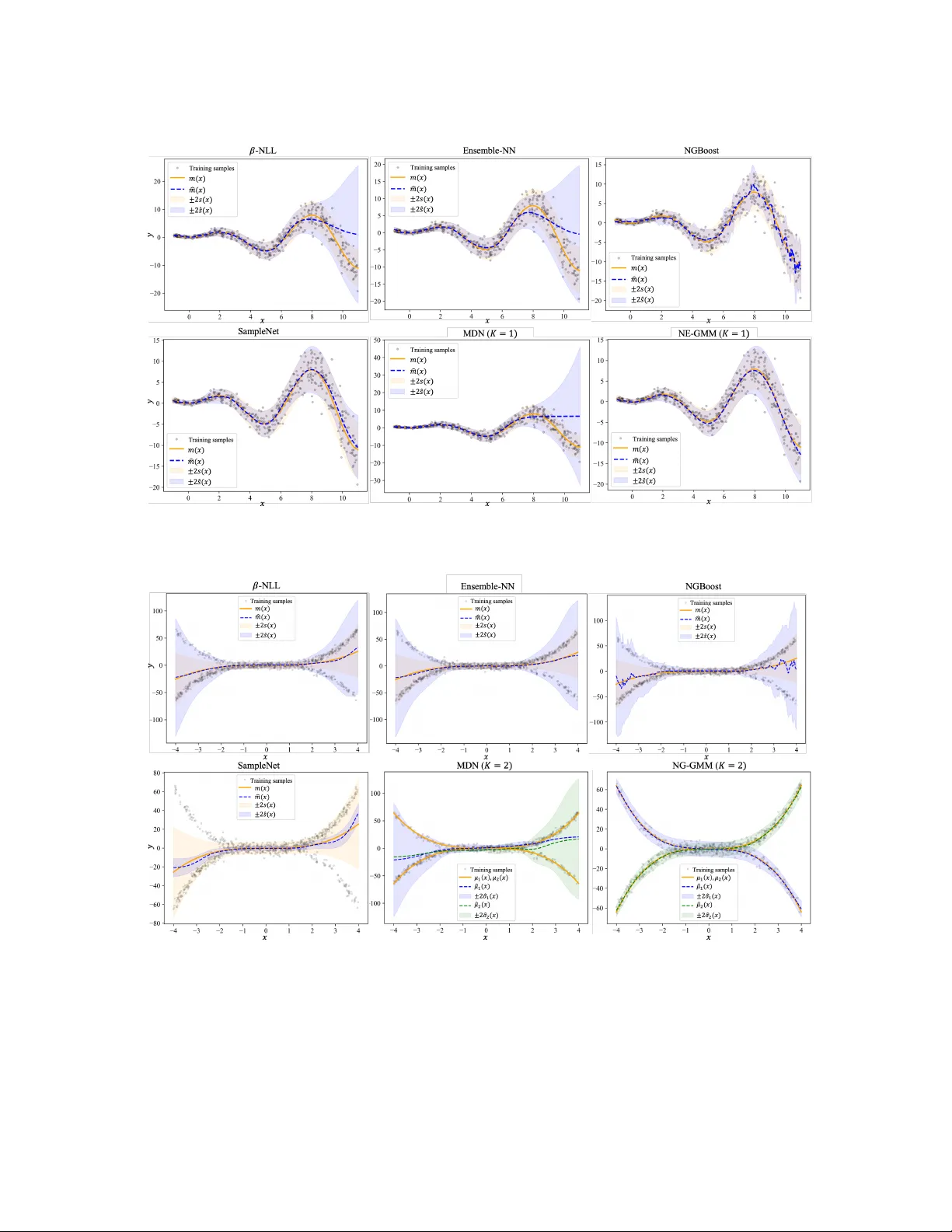
Energy Score-Guided Neural Gaussian Mixture Mo del for Predictiv e Uncertain t y Quan tiﬁcation Y ang Y ang y angy ang.st a t@gmail.com Scho ol of Statistics and Data Scienc e Nankai University Tianjin, China Ch unlin Ji chunlin.ji@kuang-chi.com Kuang-Chi Institute of A dvanc e d T e chnolo gy Shenzhen, China Hao y ang Li hao y ang-comp.li@pol yu.edu.hk Dep artment of Computing The Hong Kong Polyte chnic University Hong Kong SAR, China Ke Deng kdeng@tsinghua.edu.cn Dep artment of Statistics and Data Scienc e Tsinghua University Beijing, China Abstract Quan tifying predictive uncertain ty is essen tial for real-world mac hine learning applications, esp ecially in scenarios requiring reliable and in terpretable predictions. Man y common para- metric approaches rely on neural netw orks to estimate distribution parameters b y optimiz- ing the negativ e log-lik eliho o d. Ho wev er, these metho ds often encounter c hallenges like training instability and mode collapse, leading to po or estimates of the mean and v ariance of the target output distribution. In this w ork, w e propose the Neural Energy Gaussian Mixture Model (NE-GMM), a nov el framew ork that in tegrates Gaussian Mixture Mo del (GMM) with Energy Score (ES) to enhance predictive uncertaint y quantiﬁcation. NE- GMM lev erages the ﬂexibilit y of GMM to capture complex m ultimo dal distributions and lev erages the robustness of ES to ensure well-calibrated predictions in diverse scenarios. W e theoretically prov e that the hybrid loss function satisﬁes the properties of a strictly prop er scoring rule, ensuring alignmen t with the true data distribution, and establish gen- eralization error b ounds, demonstrating that the model’s empirical performance closely aligns with its exp ected p erformance on unseen data. Extensive exp erimen ts on b oth syn- thetic and real-w orld datasets demonstrate the sup eriorit y of NE-GMM in terms of both predictiv e accuracy and uncertaint y quantiﬁcation. Keyw ords: Uncertain ty quantiﬁcation, Gaussian mixture model, energy score, general- ization error, trustable machine learning 1 In tro duction Predictiv e uncertain ty quantiﬁcation (UQ) is a cen tral requirement in mo dern machine learning systems that op erate under distributional shift, limited sup ervision, or high-stakes decision m aking, including weather forecasting, healthcare, autonomous driving, and ﬁnan- cial mark ets (Smith, 2014; Ab dar et al., 2021; Huang et al., 2024; Zhang et al., 2025). In 1 suc h applications, a p oin t prediction alone is often insuﬃcient: do wnstream actions (e.g., allo cating medical resources, triggering safety in terven tions, or managing p ortfolio risk) t yp- ically depend on calibrated measures of uncertain t y , suc h as predictiv e in terv als, tail risks, or probabilities of constrain t violations. Uncertain ty in machine learning mo dels can be broadly categorized in to tw o types: epistemic uncertain t y , which arises from mo del limitations and data scarcity , and aleatoric uncertain ty , which stems from inheren t random noise in the data (Amini et al., 2020; H ¨ ullermeier and W aegeman, 2021; Lahlou et al., 2023; Mucs´ an yi et al., 2024; Smith et al., 2025). Epistemic uncertaint y can be reduced with more data or impro ved mo dels, while aleatoric uncertain ty is irreducible. In regression tasks, aleatoric uncertain ty can further b e classiﬁed as homoscedastic (constant v ariance) or heteroscedastic (input-dep enden t v ari- ance). T raditional regression metho ds, like linear regression, often assume homoscedastic noise, limiting their applicabilit y in real-w orld settings with v arying noise lev els. T o address heteroscedastic noise, metho ds based on the negativ e log-likelihoo d (NLL) of a Gaussian distribution are widely used. F or example, ensem ble of neural net w orks (NNs) (Lakshminara yanan et al., 2017) hav e b een prop osed to improv e robustness. How ever, NLL optimization often suﬀers from “ric h-get-richer” eﬀect, where low-v ariance regions domi- nate the training pro cess, leading to degraded p erformance in high-v ariance regions (Sk afte et al., 2019; Duan et al., 2020; Maximilian et al., 2022). T o mitigate this issue, v arian ts suc h as β -NLL (Maximilian et al., 2022) and reliable training sc hemes (Sk afte et al., 2019) rew eight sample con tributions during NLL optimization. NGBo ost emplo ys a multiparam- eter bo osting algorithm with the natural gradient to eﬃcien tly learn the distributions, but exhibits unsmo oth oscillations due to the decision-tree base learners, whic h are inherently piecewise constant across the feature space (Duan et al., 2020). F urthermore, all these metho ds rely on a single Gaussian-based lik eliho od ob jectiv e, which can b e o verly sensitive to lo cal v ariance collapse, and they lac k rigorous theoretical analysis. Ba y esian approac hes, suc h as Bay esian Neural Netw orks (BNNs) (Kendall and Gal, 2017; Gawlik owski et al., 2023) and Mon te Carlo dropout (Gal and Ghahramani, 2016), in tro duce priors o ver neural net work parameters to achiev e UQ. While theoretically app ealing, these Ba y esian methods often come with high computational costs and training instability . Moreov er, all the afore- men tioned metho ds face challenges in eﬀectiv ely mo deling complex non-Gaussian data and m ultimo dal structures. Mixture Densit y Netw orks (MDN) (Bishop, 1994) oﬀer greater ﬂexibilit y by mo deling the output as a Gaussian Mixture Model (GMM), with mo del parameters learned via neural net works. While MDNs can represen t multimodality , they are prone to mo de collapse and training instabilities, particularly when optimized purely by NLL, and it still aﬀected b y the “ric h-get-richer” eﬀect. An alternativ e line of w ork lev erages prop er scoring rules deﬁned on samples to train predictive distributions. A prominent example is the Energy Score (ES), whic h ev aluates distributions through exp ectations of pairwise distances and is applicable in m ultiv ariate settings (Gneiting and Raftery, 2007). Harakeh et al. (2023) prop osed SampleNet, a nonparametric approac h that treats neural netw ork outputs as empirical distributions and employs ES as the training loss to ev aluate predictiv e distributions. While this metho d demonstrates strong calibration prop erties, it suﬀers from high computational costs of O ( M 2 ) due to Monte Carlo sampling, where M is the n umber of samples, and lac ks an explicit parametric structure, limiting b oth interpretabilit y and computational eﬃciency . 2 This pap er prop oses the Neur al Ener gy Gaussian Mixtur e Mo del (NE-GMM) , whic h com bines the structural ﬂexibilit y of Input-dep enden t Gaussian Mixture Model (IGMM) with the calibration b eneﬁts of the Energy Score. Our k ey idea is to train an IGMM using a hybrid loss that interpolates b et ween NLL and ES. The NLL comp onen t encourages a compact parametric representation with eﬃcien t inference, whereas the ES comp onen t acts as a stabilizing regularizer that mitigates mo de collapse and promotes diversit y across mixture components. In summary , our con tributions are as follows: (1) W e in tro duce NE-GMM, an energy-score-guided IGMM trained using a h ybrid scoring rule, com bining eﬃcien t parametric inference with impro v ed calibration. (2) W e deriv e an analytic expression of the energy score under IGMM (with K mix- tures), resulting in an eﬃcient O ( K 2 ) training ob jective, which is signiﬁcan tly more computationally eﬃcien t than SampleNet’s O ( M 2 ) complexit y when M ≫ K . (3) W e pro vide theoretical guaran tees: (i) the hybrid score is strictly prop er under mild conditions; (ii) the induced learning ob jectiv e admits generalization error bounds that connect empirical and p opulation risks. (4) W e e mpirically demonstrate, on syn thetic and real-world b enc hmarks, that NE-GMM impro ves b oth predictive accuracy and uncertaint y quan tiﬁcation compared to state- of-the-art approac hes. The remainder of the paper is organized as follows. Section 2 pro vides background on parametric approaches for UQ, including the single Gaussian distribution, Gaussian mixture mo del, and energy score. Section 3 introduces the prop osed NE-GMM framework, detailing the h ybrid loss and statistical inference. The theoretical analysis of the hybrid loss is presen ted in Section 4. Experimental results on b oth syn thetic and real-world b enc hmarks are reported in Section 5, follo wed by concluding remarks in Section 6. 2 Bac kgrounds and Preliminaries W e consider a regression task with a d -dimensional input x ∈ X ⊂ R d , where X is the input space, and the output y ∈ R . Let D = { ( x i , y i ) } N i =1 represen t a set of i.i.d. training samples. The goal is to design a mo del that accurately predicts y giv en its corresp onding input x , while also providing reliable estimates of predictive uncertaint y . 2.1 Single Gaussian Distribution W e assume the conditional distribution of y giv en x follo ws a Gaussian distribution: p ( y | x ) = ϕ ( y ; µ ( x ) , σ 2 ( x )) , (1) where ϕ ( . ; µ ( x ) , σ 2 ( x )) is the probabilit y density function of the Gaussian distribution with mean µ ( x ) and v ariance σ 2 ( x ). The v ariance σ 2 ( x ) quan tiﬁes the uncertaint y of the mo del. F or an observ ation y sampled from a distribution F with f ( · ) as its probability density function, the lo garithmic sc or e of F with resp ect to y is deﬁned as S l ( F , y ) = − log f ( y ) . (2) The Gaussian distribution in (1) is determined b y µ ( . ) and σ ( . ), and neural net works are often used to parameterize these functions. Let ψ denote the neural netw ork parameters 3 for µ ( . ) and σ ( . ), and denote the corresp onding Gaussian distribution as F g ψ ( · ). Assuming D = { ( x i , y i ) } N i =1 is i.i.d. and generated from (1), the negativ e log-lik eliho o d (NLL) loss for D is deﬁned as: L l, D ( F g ψ ) = 1 N N X i =1 S l ( F g ψ ( x i ) , y i ) , (3) where S l ( F g ψ ( x ) , y ) = log( σ ( x )) + ( y − µ ( x )) 2 2 σ 2 ( x ) + const. The partial deriv ativ es of S l ( F g ψ ( x ) , y ) with resp ect to µ ( x ) and σ ( x ) are ∂ S l ∂ µ ( x ) = µ ( x ) − y σ 2 ( x ) , (4) ∂ S l ∂ σ ( x ) = σ 2 ( x ) − ( µ ( x ) − y ) 2 σ 3 ( x ) . Due to the presence of σ ( x ) in the denominator of (4), the gradients of the NLL loss L l, D tend to scale more hea vily for lo w-v ariance data p oints, where σ ( x ) is close to 0. This inherently biases the single Gaussian mo del to fo cus on lo w-noise regions, prioritizing accurate predictions in those areas while p oten tially neglecting high-v ariance regions. This phenomenon is commonly referred to as the “ric h-get-ric her” eﬀect, whic h can lead to sub optimal uncertaint y quantiﬁcation (Sk afte et al., 2019; Duan et al., 2020; Maximilian et al., 2022; Stirn et al., 2023). 2.2 Gaussian Mixture Mo del A Gaussian Mixture Mo del (GMM) is a probability distribution expressed as a weigh ted sum of K Gaussian comp onen ts (Lindsa y, 1995; Ev eritt, 2013; McLac hlan et al., 2019). The probabilit y densit y function of an observ ation y from a GMM is deﬁned as: p ( y ) = K X k =1 π k ϕ ( y ; µ k , σ 2 k ) , (5) where ϕ ( . ; µ k , σ 2 k ) denotes the probabilit y density function of the k -th Gaussian comp onen t with mean µ k and v ariance σ 2 k , { π k } K k =1 are w eights satisfying P K k =1 π k = 1 and 0 < π k < 1 for each k , and θ = { ( π k , µ k , σ k ) } K k =1 is the complete set of GMM parameters. These parameters are typically estimated using the Exp ectation-Maximization (EM) algorithm (Dempster et al., 1977; McLac hlan and Basford, 1988; McLac hlan et al., 2019). When the output y dep ends on an input x , the GMM in (5) can b e extended to an Input-dep enden t GMM (IGMM) for UQ in regression: p ( y | x ) = K X k =1 π k ( x ) ϕ ( y ; µ k ( x ) , σ 2 k ( x )) , (6) where P K k =1 π k ( x ) = 1 , 0 < π k ( x ) < 1 for all x ∈ X and k , and the parameters θ in GMM are replaced b y x -dependent parameters θ ( x ) = { ( π k ( x ) , µ k ( x ) , σ k ( x )) } K k =1 , whic h 4 v ary with x . Bishop (1994) prop osed using neural net works, parameterized by ψ , to map x to the corresponding IGMM parameters θ ( x ). Here θ ( x ) dep ends on ψ and is denoted as F ψ ( x ), whic h forms the basis of the so-called Mixture Densit y Net works (MDN) (Bishop, 1994). The function F ψ ( . ) outputs a 3 K -dimensional vector containing all the parameters of IGMM. Since the output F ψ ( . ) deﬁnes the IGMM, which mo dels the conditional distribution of y | x , w e also use F ψ ( . ) to refer to the IGMM distribution itself when there is no am biguity . Giv en a set of samples i.i.d. D = { ( x i , y i ) } N i =1 from an IGMM c haracterized b y param- eters F ψ ( · ), the NLL loss for D is deﬁned as: L l, D ( F ψ ) = 1 N N X i =1 S l ( F ψ ( x i ) , y i ) , (7) where S l ( F ψ ( x ) , y ) = − log K X k =1 π k ( x ) ϕ ( y ; µ k ( x ) , σ 2 k ( x )) ! , and ϕ ( . ; µ k ( x ) , σ 2 k ( x )) is the probability densit y function of N ( µ k ( x ) , σ 2 k ( x )). Here π k ( . ), µ k ( . ) and σ k ( . ) are determined b y the neural netw ork parameters ψ . Prop osition 1. The p artial derivatives of S l ( F ψ ( x ) , y ) with r esp e ct to π k ( x ) , µ k ( x ) , and σ k ( x ) in an IGMM ar e given by: ∂ S l ∂ π k ( x ) = − r k ( x ) , ∂ S l ∂ µ k ( x ) = µ k ( x ) − y σ 2 k ( x ) π k ( x ) r k ( x ) , (8) ∂ S l ∂ σ k ( x ) =  1 σ k ( x ) − ( µ k ( x ) − y ) 2 σ 3 k ( x )  π k ( x ) r k ( x ) , wher e r k ( x ) = ϕ ( y ; µ k ( x ) , σ 2 k ( x )) P K l =1 π l ( x ) ϕ ( y ; µ l ( x ) , σ 2 l ( x )) . Lemma 2. The T aylor exp ansions of the p artial derivative functions of S l ( F ψ ( x ) , y ) as σ k ( x ) → ∞ ar e: ∂ S l ∂ π k ( x ) = − 1 √ 2 π T 1 · 1 σ k ( x ) + π k ( x ) 2 π T 2 1 · 1 σ 2 k ( x ) + O  1 σ 3 k ( x )  , ∂ S l ∂ µ k ( x ) = π k ( x )( µ k ( x ) − y ) √ 2 π T 1 · 1 σ 3 k ( x ) + O  1 σ 4 k ( x )  , (9) ∂ S l ∂ σ k ( x ) = π k ( x ) √ 2 π T 1 · 1 σ 2 k ( x ) + O  1 σ 3 k ( x )  , 5 wher e T 1 = X l  = k π l ( x ) ϕ ( y ; µ l ( x ) , σ 2 l ( x )) . The r esults holds for T 1  = 0 ; otherwise, those functions r e duc e to the single Gaussian c ase. F rom Lemma 2, the gradients S l can either v anish or explo de as σ k ( · ) v aries. Compared with the single Gaussian case in tro duced in Section 2.1, the terms ∂ S l ∂ µ k ( x ) and ∂ S l ∂ σ k ( x ) tend to 0 more quic kly as σ k ( x ) → ∞ in the IGMM setting. This exacerbates the rich-get-ric her eﬀect. F urthermore, the v anishing or exploding gradien ts caused by ∂ S l ∂ π k ( x ) will cause mo de collapse when m ultiple mixture comp onen ts to con verge to the same data mo de. In this scenario, w ell-ﬁtted comp onen ts dominate gradien t up dates, eﬀec tiv ely starving other comp onen ts, whic h ev en tually die out. As a result, the model fails to capture the full m ultimo dalit y inheren t in the ov erall distribution. Without appropriate regularization, early stopping, or other mitigation tec hniques, existing metho ds like MDN are particularly prone to o verﬁtting and training instability , especially when trained on small or noisy datasets. 2.3 Energy Score Energy Score (ES) is a statistical to ol designed to ev aluate the qualit y of a predictiv e distribution F for a target v alue y b y assessing the alignment b et w een F and y as follows: S e ( F , y ) = E z ∼ F ∥ z − y ∥ − 1 2 E z ,z ′ ∼ F ∥ z − z ′ ∥ , (10) where z and z ′ are indep enden t random v ariables from F , || x || represents the Euclidean norm of the v ector x , and the exp ectations are tak en with respect to z and z ′ , with y treated as a ﬁxed constant. The ﬁrst term in S e measures the compatibilit y b et ween F and y , while the second term p enalizes ov erconﬁdence in F b y encouraging diversit y among its samples. By in tegrating these tw o terms, the energy score balances prediction accuracy with div ersit y in the predicted distribution F (Gneiting and Raftery, 2007). If the target v alue y comes from a distribution Q , w e can deﬁne the exp ected version of ES with resp ect to Q as S e ( F , Q ) = E y ∼ Q S e ( F , y ) = E y ∼ Q,z ∼ F ∥ z − y ∥ − 1 2 E z ,z ′ ∼ F ∥ z − z ′ ∥ , (11) where z , z ′ ∼ F and y ∼ Q are all indep enden t random v ariables, and the exp ectations are tak en o ver all in volv ed random v ariables. F or a set of target v alues { y 1 , · · · , y N } , w e can deﬁne the sample av eraged v ersion of ES b elo w as a loss function (referred to as the ES loss) to guide the training of the predictive distribution F ψ parametrized b y the neural net work parameters ψ : L e, D ( F ψ ) = 1 N N X i =1 S e ( F ψ ( x i ) , y i ) . (12) The ES loss is highly ﬂexible, enabling it to capture div erse predictive uncertainties dep ending on the choice of the distribution F ψ . Ho wev er, its performance hea vily relies 6 on the correct selection of F ψ . Moreo ver, when F ψ is complex, the ES loss in (12) has no closed form which often dep ends on using Monte Carlo tec hniques. F or example, Harakeh et al. (2023) introduced SampleNet, which optimizes a neural netw ork prediction mo del F ψ with the following approximated ES loss: ˆ L e, D ( F ψ ) = 1 N N X i =1 ˆ S e ( F M ψ ( x i ) , y i ) , with S e replaced b y its Monte Carlo v ersion ˆ S e ( F M ψ ( x i ) , y i ) = 1 M M X m =1 ∥ z ( m ) i − y i ∥ − 1 2 M 2 M X m,n =1 ∥ z ( m ) i − z ( n ) i ∥ . Here, F M ψ denotes the empirical distribution from M samples { z (1) i , . . . , z ( M ) i } obtained b y outputs of the mo del F ψ . Because the Mon te Carlo appro ximation ˆ S e has a computational complexit y of O ( M 2 ), SampleNet is computationally expensive. 3 Metho d In this work, w e propose the Neural Energy Gaussian Mixture Mo del (NE-GMM), a no vel framew ork that integrates unique adv antages of IGMM and ES for more eﬃcien t prediction with UQ. 3.1 NE-GMM with a Hybrid Loss The con v entional MDN mo dels y using an IGMM which often leads to the ric h-get-richer eﬀect. The prop osed NE-GMM aims to address this limitation by enhancing the MDN framew ork. It incorp orates an additional ES loss as a regularization term alongside the NLL loss. Unlik e the existing metho d SampleNet, whic h relies on an appro ximated ES loss, our approac h fo cuses on utilizing the exact ES loss L e, D ( F ψ ) in (12). Since F ψ ( x ) is an IGMM, the analytic form of S e ( F ψ ( x ) , y i ) can b e con v eniently derived, as sho wn in the follo wing theorem. Theorem 3 (Analytic form of energy score) Given the distribution derive d fr om an IGMM F ψ ( · ) , the ES loss is S e ( F ψ ( x ) , y ) = K X m =1 π k ( x ) A m ( x, y ) − 1 2 K X m =1 K X l =1 π m ( x ) π l ( x ) B ml ( x ) , wher e A m ( x, y ) = σ m ( x ) r 2 π e − ( µ m ( x ) − y ) 2 2 σ 2 m ( x ) + ( µ m ( x ) − y )  2Φ  µ m ( x ) − y σ m ( x )  − 1  , B ml ( x ) = q σ 2 m ( x ) + σ 2 l ( x ) r 2 π e − ( µ m ( x ) − µ l ( x ) ) 2 2 ( σ 2 m ( x )+ σ 2 l ( x ) ) +( µ m ( x ) − µ l ( x ))   2Φ   µ m ( x ) − µ l ( x ) q σ 2 m ( x ) + σ 2 l ( x )   − 1   . 7 The calculation of S e ( F ψ ( x ) , y ) with the computational complexit y of O ( K 2 ) is signiﬁcan tly more eﬃcien t than the O ( M 2 ) complexit y in SampleNet for M ≫ K . Using the expression of S e deriv ed in Theorem 3, we can obtain the follo wing results for the partial deriv ativ es of S e with respect to π k ( x ), µ k ( x ) and σ k ( x ). Prop osition 4 (P artial deriv ativ es of S e ) ∂ S e ∂ π k ( x ) = A k ( x, y ) − K X l =1 π l ( x ) B kl ( x ) , ∂ S e ∂ µ k ( x ) = π k ( x ) (2Φ( w k ) − 1) − K X l =1 π l ( x ) (2Φ( w kl ) − 1) ! , ∂ S e ∂ σ k ( x ) = 2 π k ( x )   ϕ ( w k ) − K X l =1 π l ( x ) σ k ( x ) q σ 2 k ( x ) + σ 2 l ( x ) ϕ ( w kl )   , wher e w k = µ k ( x ) − y σ k ( x ) , w kl = µ k ( x ) − µ l ( x ) √ σ 2 k ( x )+ σ 2 l ( x ) . T o further understand the behavior of the gradients of S e , w e compute their T aylor expansions. Lemma 5. As σ k ( x ) → ∞ , ∂ S e ∂ π k ( x ) = ( √ 2 − 2) π k ( x ) √ π · σ k ( x ) + T 2 √ 2 π · 1 σ k ( x ) + O  1 σ 3 k ( x )  , ∂ S e ∂ µ k ( x ) = r 2 π T 3 π k ( x ) · 1 σ k ( x ) + O  1 σ 2 k ( x )  , ∂ S e ∂ σ k ( x ) = √ 2 − 1 √ π π 2 k ( x ) − T 2 π k ( x ) √ 2 π · 1 σ 2 k ( x ) + O  1 σ 4 k ( x )  , wher e T 2 = ( µ k ( x ) − y ) 2 − X l  = k π l ( x )( σ 2 l ( x ) + ( µ k ( x ) − µ l ( x )) 2 ) , T 3 = µ k ( x ) − y − K X l  = k π l ( x )( µ k ( x ) − µ l ( x )) . Lemma 5 rev eals several key properties: ∂ S e ∂ π k ( x ) → ∞ as σ k ( x ) → ∞ , implying that the ES loss S e places increased emphasis on high-v ariance regions when optimizing π k ( x ). This ensures that comp onen ts and data p oin ts with higher v ariance are not neglected during optimization. ∂ S e ∂ σ k ( x ) → √ 2 − 1 √ π π 2 k ( x ) > 0 as σ k ( x ) → ∞ . These results indicate that the partial deriv atives with resp ect to π k ( x ) and σ k ( x ) do not exhibit the rich-get-ric her eﬀect, whic h is an issue for the NLL loss S l in an IGMM. Although ∂ S e ∂ µ k ( x ) → 0 as σ k ( x ) → ∞ , the deca y is signiﬁcantly slow er compared to ∂ S l ∂ µ ( x ) in a single Gaussian distribution (see 8 (4)) or ∂ S l ∂ µ k ( x ) in an IGMM (see (8)). This slow er deca y ensures that the ES loss remains eﬀectiv e in mitigating the rich-get-ric her eﬀect during training. These ﬁndings conﬁrm that training neural net works with the ES loss eﬀectively ensures all mixture comp onen ts con tribute meaningfully to the ﬁnal predictiv e distribution. T o leverage the complemen tary strengths of the NLL loss L l, D ( F ψ ) and the ES loss L e, D ( F ψ ), w e propose a h ybrid loss for the predictiv e model F ψ : L h, D ( F ψ ) = η · L l, D ( F ψ ) + (1 − η ) · L e, D ( F ψ ) = 1 N N X i =1 S h ( F ψ ( x i ) , y i ) , (13) where η ∈ [0 , 1] is a w eighting parameter that balances the con tributions of the NLL loss and the ES loss, and S h ( F , y ) = η · S l ( F , y ) + (1 − η ) · S e ( F , y ) (14) is a hybrid score based on the w eigh ted av erage of S l and S e . Hereinafter, w e refer to the IGMM equipped with the ab o ve energy score as the Neural Energy Gaussian Mixture Mo del (NE-GMM). The prop osed NE-GMM can b e trained b y minimizing the h ybrid loss L h, D ( F ψ ). Apparently , the NE-GMM degenerates to to the MDN framew ork with the NLL loss only when η = 1, and fo cuses en tirely on the ES loss when η = 0. This hybrid framew ork generalizes and uniﬁes the t wo approac hes, lev eraging their re- sp ectiv e strengths. The NLL loss ensures that the mo del learns a parametric represen tation of the predictiv e distribution, capturing the primary complex and m ultimo dal structure of the data under the framew ork of MDN. Meanwhile, the ES loss addresses the limitations of MDN by promoting div ersit y in the predicted samples, ensuring that the mo del mitigates the rich-get-ric her eﬀect and a v oids mode collapse to capture uncertain ty more robustly . The com bined loss function in (13) allo ws the mo del to learn structured and interpretable predictiv e distributions while encouraging robustness and div ersity in its predictions. This mak es the framework particularly well-suited for applications requiring accurate and reliable represen tations of complex uncertainties. 3.2 Prediction with UQ based on NE-GMM Once trained, NE-GMM pro vides a fully sp eciﬁed IGMM for an y new input x . This para- metric represen tation enables eﬃcien t computation of standard predictiv e summaries used in regression with UQ. F or an IGMM, the predictive mean and predictive v ariance can b e written in closed form (Bishop, 1994): m ( x ) = E [ y | x ] = K X k =1 π k ( x ) µ k ( x ) , (15) s 2 ( x ) = V ar[ y | x ] = K X k =1 π k ( x )  σ 2 k ( x ) + ( µ k ( x ) − m ( x )) 2  . The expression for s 2 ( x ) highligh ts t w o complemen tary sources of uncertaint y: the within- comp onen t v ariance σ 2 k ( x ) (local noise) and the b et ween-component disp ersion ( µ k ( x ) − m ( x )) 2 (m ultimo dalit y/mixture uncertain ty). 9 In NE-GMM, the functions ( π k ( . ) , µ k ( . ) , σ k ( . )) are parameterized b y a neural netw ork with parameters ψ . After training, w e obtain ˆ ψ by minimizing the hybrid loss L h, D ( F ψ ). F or an y new x , w e ev aluate F ˆ ψ ( x ) = { ( π k ( x ; ˆ ψ ) , µ k ( x ; ˆ ψ ) , σ k ( x ; ˆ ψ )) } K k =1 and compute m ( x ) and s 2 ( x ) via (15). In practice, m ( x ) is used as the point prediction, while s ( x ) provides a scale of predictive uncertaint y . When full predictive interv als are needed, NE-GMM also supp orts eﬃcien t sampling from the mixture: for eac h x , sample a comp onen t index k ∼ Categorical( π 1 ( x ) , . . . , π K ( x )) and then sample y ∼ N ( µ k ( x ) , σ 2 k ( x )). This allo ws us to approximate predictiv e quan tiles and interv al estimates at arbitrary conﬁdence lev els without sacriﬁcing the interpretabilit y of the parametric mixture. 4 Theoretical Results This section develops theoretical supports for NE-GMM from t wo complementary p erspec- tiv es. First, we sho w that the h ybrid score S h corresp onds to a strictly pr op er scoring rule, implying that, at the p opulation lev el, minimizing the exp ected h ybrid loss reco vers the true conditional distribution. Second, w e pro vide a ﬁnite-sample generalization guarantee that controls the gap b et ween empirical and exp ected risks o ver the function class induced b y the neural netw ork parameterization. Considering probabilistic forecasts on a general sample space Ω. Let A b e a σ -algebra of subsets of Ω, and P be a conv ex class of probability measures on the measurable space (Ω , A ). Deﬁnition 6. A r e al value function S : P × Ω → R is “ P -quasi-inte gr able” for every F ∈ P if the inte gr al S ( F , Q ) = R S ( P , y ) dQ ( y ) exists for al l F, Q ∈ P , though it may not ne c essarily b e ﬁnite. Deﬁnition 7. A r e al value function S : P × Ω → R is c al le d a “sc oring rule” if S ( F , · ) is P -quasi-inte gr able for al l F ∈ P . Deﬁnition 8. A sc oring rule S is “pr op er” r elative to P if S ( Q, Q ) ≤ S ( F , Q ) , ∀ F , Q ∈ P , (16) and is “strictly pr op er” r elative to P if (16) holds with e quality if and only F = Q . Theorem 9. Supp ose b oth S l and S e ar e P -quasi-inte gr able, the hybrid sc or e S h in (14) is a strictly pr op er sc oring rule. Theorem 9 formalizes the k ey design principle of NE-GMM: com bining NLL (logarithmic score) with ES preserves the compatibilit y prop erty of prop er scoring rules, ensuring that the optimization of the h ybrid loss eﬀectively approximates the true distribution. The remaining results focus on ﬁnite-sample guarantees for minimizing the empirical h ybrid loss. W e state in termediate steps explicitly to clarify the role of eac h statem en t: Assumption 1 prev ents degenerate parameters and pro vides tail control for y ; Lemma 10 es- tablishes high-probabilit y concen tration properties for y that allo w us to w ork on a bounded 10 ev ent; Lemmas 13 – 14 sho w that the p er-sample scores are Lipschitz on that even t, enabling a contraction argumen t; Theorem 15 then b ounds the p opulation–empirical h ybrid risk gap b y the Rademac her complexit y of the underlying neural netw ork parameter class. T o further inv estigate the theoretical prop erties of NE-GMM in mo del complexit y and training loss of NE-GMM, w e in tro duce the follo wing assumption and deﬁnitions. Assumption 1. The me an functions and varianc e functions in the IGMM ar e b ounde d: | µ k ( x ) | ≤ M µ and σ 2 k ( x ) ∈ [ σ 2 min , σ 2 max ] for al l k and x ∈ X , wher e M µ > 0 , σ max ≥ σ min > 0 . The ab o ve assumptions for µ k ( . ) and σ 2 k ( . ) can b e easily satisﬁed by adding truncation on the outputs of the neural netw orks. Lemma 10. Under Assumption 1, for any α ∈ (0 , 1) , ther e exists M c = 2 M µ + σ max p 2 log(2 /α ) > 0 , such that P ( | y − µ k ( x ) | ≥ M c ) ≤ α, for al l k and x ∈ X . Deﬁnition 11. L et G b e a class of r e al-value d functions mapping fr om X to R , and A = { a 1 , . . . , a N } ar e samples fr om X . The empiric al R ademacher c omplexity of G is deﬁne d as: ˆ R A ( G ) = E ξ " sup g ∈G 1 N N X i =1 ξ i g ( a i ) !# , wher e ξ 1 , . . . , ξ N ar e R ademacher variables, which ar e indep endent uniformly chosen fr om { -1,1 } . Deﬁnition 12. The R ademacher c omplexity of G is deﬁne d as the exp e ctation of the em- piric al R ademacher c omplexity over the samples A : R N ( G ) = E A h ˆ R A ( G ) i . T o connect statistical complexity of the neural parameterization to the complexity of the induced loss, w e require the scoring functions to b e stable under small p erturbations of the predicted mixture parameters. Lemmas 13 and 14 provide this stability in the form of high-probability Lipschitz b ounds. These b ounds are key for applying a con traction inequalit y in the Rademac her complexit y analysis: they allow us to control the complexit y of the comp osed class ( x, y ) 7→ S h ( F ψ ( x ) , y ) by that of x 7→ F ψ ( x ). Lemma 13 (Lipsc hitz con tinuit y of S l ) Under Assumption 1, for any α ∈ (0 , 1) , ther e exists a c onstant C l > 0 such that the fol lowing holds with pr ob ability at le ast 1 − α : ∥ S l ( F ψ ( x ) , y ) − S l ( F ψ ( x ′ ) , y ′ ) ∥ 1 ≤ C l ∥ ( F ψ ( x ) , y ) − ( F ψ ( x ′ ) , y ′ ) ∥ 1 . (17) Lemma 14 (Lipsc hitz con tinuit y of S e ) Under Assumption 1, for any α ∈ (0 , 1) , ther e exists a c onstant C e > 0 such that the fol lowing holds with pr ob ability at le ast 1 − α : ∥ S e ( F ψ ( x ) , y ) − S e ( F ψ ( x ′ ) , y ′ ) ∥ 1 ≤ C e ∥ ( F ψ ( x ) , y ) − ( F ψ ( x ′ ) , y ′ ) ∥ 1 . (18) 11 Let F be the class of functions that map X to R 3 K . W e can then apply symmetriza- tion and concentration to obtain a uniform b ound on the deviation b etw een exp ected and empirical h ybrid risks ov er the function class F . Theorem 15. F or any δ ∈ (0 , 1) , with pr ob ability at le ast 1 − δ , the fol lowing ine quality holds for al l F ψ ∈ F : E [ L h, D ( F ψ )] − L h, D ( F ψ ) ≤ 4 C h R N ( F ) + M h r log(1 /δ ) 2 N , for some C h > 0 and M h > 0 . Theorem 15 shows that the generalization error is b ounded by the neural net w ork’s complexit y (measured b y R N ( F )) and the dataset size N . R N ( F ) dep ends on the input di- mension and the neural net w ork architecture, including its depth, width, weigh t norms, and activ ation function. These aspects ha v e b een extensively studied in prior work Neyshabur et al. (2015); Golo wic h et al. (2018) and Galan ti et al. (2023), and are not the primary fo cus of our analysis here. 5 Exp erimen ts T o ev aluate the p erformance of the proposed NE-GMM, we conduct experiments on tw o to y regression tasks with heteroscedastic or m ultimo dal noises follo wing similar settings as in Harak eh et al. (2023) and El-Laham et al. (2023), and tw o widely used real-world prediction tasks for UCI regression (Hernandez-Lobato and Adams, 2015) and ﬁnancial time series forecasting (El-Laham et al., 2023). The p erformance of NE-GMM is compared to ﬁv e comp eting metho ds, including β -NLL (Maximilian et al., 2022), ensem ble neural net works (Ensem ble-NN) (Lakshminaray anan et al., 2017), NGBo ost (Duan et al., 2020), MDN (Bishop, 1994), and SampleNet (Harak eh et al., 2023). Hyp erparameters of the in volv ed methods are pro vided in T able 7 of App endix D. 5.1 T o y Regressions W e b egin with tw o toy regression tasks to ev aluate the capability of NE-GMM in mo deling heteroscedastic and multimodal noise. • Example 1 - Heteroscedastic Noise: we assume that y ( x ) = x sin( x ) + xε 1 + ε 2 , where x ∈ [ − 1 , 11], and ε 1 , ε 2 ∼ N (0 , 0 . 09). The true mean and v ariance functions of this example are m ( x ) = x sin( x ) and s 2 ( x ) = 0 . 09( x 2 + 1), resp ectiv ely . • Example 2 - Bimo dal Noise: we assume y ( x ) = U x 3 + ε , where U ∈ {− 1 , 1 } is a random v ariable follo wing a Bernoulli distribution with P ( U = − 1) = 0 . 3, x ∈ [ − 4 , 4], and ε ∼ N (0 , 9). The true conditional distribution of y | x under this regression model is an IGMM with t wo Gaussian comp onen ts of the follo wing parameters: π = ( π 1 , π 2 ) = (0 . 3 , 0 . 7) , µ 1 ( x ) = − x 3 , µ 2 ( x ) = x 3 , σ 1 ( x ) = σ 2 ( x ) = 3. The o verall mean and v ariance function are m ( x ) = 0 . 4 x 3 and s 2 ( x ) = 9 + 0 . 138 x 6 . F or b oth examples, w e generate N training samples ( N = 600 for Example 1 and N = 1000 for Example 2), along with 0 . 2 N v alidation samples and 300 test samples. Since 12 the true mean function m ( · ) and standard deviation function s ( · ) are kno wn, we ev aluate the ro ot mean squared error (RMSE) for m ( · ) and s ( · ) on the test sets. The batch size is set to 32, and all metho ds use a single-lay er neural netw ork with 50 hidden units and T anh activ ations as feature extractors. The learning rate, c hosen from { 0 . 001 , 0 . 005 , 0 . 01 } , is tuned alongside other mo del parameters based on RMSEs of the combined m ( · ) and s ( · ) on the v alidation set. Each exp eriment is rep eated 50 times, and a v erage results are rep orted. F or Example 1, b oth SampleNet and NE-GMM substantially outp erform purely likelihoo d- based approac hes ( β -NLL, Ensem ble-NN, NGBoost, and MDN) in estimating m ( · ) and s ( · ). Imp ortan tly , NE-GMM achiev es the b est ov erall p erformance, improving the RMSE of the mean estimator b y 5.7% and the RMSE of the standard deviation estimator by 78.2% com- pared to the second-best SampleNet (T able 1). Figure 1 further illustrates that NE-GMM main tains high robustness even in regions with high v ariance. In Example 2, the exp erimen tal setup is sp eciﬁcally designed to ev aluate the abilit y of metho ds to represen t and learn multimodality . Metho ds that predict a single paramet- ric distribution or rely solely on sample-based forecasts without explicit mixture comp o- nen ts ( β -NLL, Ensem ble-NN, NGBo ost, and SampleNet) are unable to iden tify comp onen t- sp eciﬁc parameters. These metho ds fail to recov er the bimo dal conditional distribution, as they cannot estimate the individual comp onen t means µ k ( x ) and standard deviations σ k ( x ). Consequen tly , their p erformance is assessed only on the o v erall mean m ( x ) and standard de- viation s ( x ) as shown in T able 2 and Figure 2. By contrast, NE-GMM accurately estimates the component-speciﬁc parameters. It achiev es signiﬁcan tly lo w er RMSE and successfully iden tiﬁes the individual comp onent means and standard deviations (constant functions un- correlated with x ). F urthermore, compared to a standard MDN, NE-GMM is muc h less prone to mo de collapse in this symmetric bimo dal setting. Ov erall, these toy exp erimen ts v alidate the robustness of NE-GMM in handling both heteroscedastic and m ultimo dal data. Its ability to eﬀectiv ely capture complex uncertain ty structures, including mixture represen tations, demonstrates the practical adv antages of in- corp orating the energy-score regularizer into the training process. T able 1: The RMSE of m ( · ) and s ( · ) for the toy regression example 1. β -NLL Ensem ble-NN NGBo ost SampleNet MDN NE-GMM m ( · ) 3.669 ± 1.385 3.043 ± 0.496 0.672 ± 0.063 0.454 ± 0.180 4.571 ± 0.970 0.428 ± 0.152 s ( · ) 2.354 ± 0.930 2.840 ± 0.465 0.434 ± 0.049 0.928 ± 0.205 3.734 ± 0.945 0.202 ± 0.064 T able 2: The RMSE of ( m ( · ) , s ( · ) , π ) for the toy regression example 2. β -NLL Ensem ble-NN NGBo ost SampleNet MDN NE-GMM m ( · ) 1.903 ± 0.429 2.064 ± 0.780 4.362 ± 0.862 15.054 ± 0.449 10.767 ± 4.263 1.128 ± 0.286 s ( · ) 12.535 ± 2.463 12.900 ± 1.021 12.4 ± 0.86 7.454 ± 0.897 4.735 ± 2.644 0.778 ± 0.260 π None None None None 0.382 ± 0.044 0.095 ± 0.024 13 Figure 1: Predictive distribution plots for the toy regression example 1. Figure 2: Predictive distribution plots for the toy regression example 2. 5.2 Regression on UCI Datasets T o further ev aluate the eﬀectiveness of the prop osed NE-GMM metho d, we conduct exper- imen ts on UCI benchmark datasets, whic h are widely used in the literature for real-w orld 14 regression tasks. Details ab out the datasets can b e found in App endix E.1. Each dataset is randomly split into 20 train-test splits with an 80%-20% ratio, except for the large Protein dataset, whic h is split into 5 train-test splits. Inputs and targets are standardized based on the training set, while ev aluation metrics suc h as RMSE and NLL are rep orted in the data’s original scale. Additionally , the Prediction Interv al Co v erage Probability (PICP) and Mean Prediction Interv al Width (MPIW) at a 95% conﬁdence levels are ev aluated to assess the reliability and precision of the mo del’s uncertaint y estimates. The training set is further split in to an 8:2 ratio for training and v alidation. All methods use the same netw ork arc hitecture: a single-lay er neural net work with 50 hidden units and ReLU activ ations. The mo del w as trained for up to 2,000 ep ochs with a batc h size of 32. The learning rate w as selected from { 1e-4, 5e-4, 1e-3, 5e-3, 1e-2 } based on the best RMSE on the v alidation sets. All rep orted results represent the av erage across all test splits. It is imp ortan t to note that these results are not directly comparable to those in other publications, as performance can v ary signiﬁcantly across diﬀeren t data splits. F urthermore, diﬀerences in the use of early stopping strategies may also aﬀect comparabilit y . T ables 3 and 4 summarize predictiv e accuracy and distributional ﬁt on the UCI b enc h- marks. Ov erall, NE-GMM ac hiev es the best (or tied-b est) RMSE on the ma jorit y of datasets, indicating consistently strong point prediction accuracy . In addition, NE-GMM attains b est or near-best NLL on man y datasets, suggesting that it not only predicts the mean well but also captures the conditional disp ersion eﬀectively . Ev en in cases where another metho d attains the lo w est NLL (e.g., Protein), NE-GMM remains comp etitiv e, demonstrating robustness across div erse data regimes. Bey ond RMSE and NLL, we assess calibration and sharpness through 95% prediction in terv als. App endix T ables 9 – 10 sho w that NE-GMM t ypically pro duces PICP closer to the nominal 95% while main taining relativ ely narrow MPIW. This “well-calibrated yet sharp” b eha vior is particularly desirable for uncertain ty quantiﬁcation and is consisten t with the role of the energy-score term as a calibration-orien ted regularizer. Finally , T able 11 highligh ts that NE-GMM is computationally eﬃcien t: it is substan- tially faster than Ensemble-NN and SampleNet, while b eing comparable to β -NLL and MDN. Although NGBoost is often the fastest due to its tree-based structure, it generally lags behind in RMSE and NLL. T aken together, the UCI results demonstrate that NE- GMM pro vides a fav orable trade-oﬀ among accuracy , calibrated uncertain t y , and training cost. 5.3 Financial time series forecasting W e conduct one-step-ahead forecasting for ﬁnancial time series using historical daily price data obtained from Y aho o Finance. The forecasting problem is modeled with a t w o-lay er long short-term memory (LSTM) netw ork (Ho c hreiter and Schmidh ub er, 1997), following the setup in El-Laham et al. (2023). The input consists of the closing prices of a sp eciﬁc sto c k o ver the previous 30 trading da ys, while the target is the closing price of the next trading da y . The ev aluation is conducted on three datasets, each represen ting distinct mark et regimes: • GOOG (stable market regime): Go ogle sto c k prices (Jan uary 2019 – July 2022 for training; August 2022 – Jan uary 2023 for testing). 15 T able 3: Average RMSE on the test set for UCI regression datasets (“SC” stands for Sup erconductivit y). Dataset β -NLL Ensemble-NN NGBo ost SampleNet MDN NE-GMM Boston 2.836 ± 0.277 2.676 ± 0.178 3.130 ± 0.195 2.856 ± 0.226 2.766 ± 0.195 2.556 ± 0.205 Concrete 5.381 ± 0.528 5.425 ± 0.362 7.222 ± 0.020 5.935 ± 0.507 6.029 ± 0.751 5.678 ± 0.725 Energy 1.944 ± 0.589 2.187 ± 0.266 1.952 ± 0.216 1.866 ± 0.831 1.985 ± 0.297 1.806 ± 0.092 Kin8nm 0.08 ± 0.003 0.083 ± 0.003 0.197 ± 0.001 0.141 ± 0.070 0.082 ± 0.001 0.078 ± 0.001 Na v al 0.002 ± 0.000 0.004 ± 0.002 0.009 ± 0.000 0.003 ± 0.001 0.001 ± 0.000 0.001 ± 0.000 Protein 4.072 ± 0.048 4.656 ± 0.386 5.280 ± 0.033 4.370 ± 0.098 4.070 ± 0.051 4.014 ± 0.052 SC 12.588 ± 0.440 13.010 ± 0.226 17.377 ± 0.288 11.943 ± 0.091 11.515 ± 0.141 11.034 ± 0.078 WineRed 0.646 ± 0.037 0.637 ± 0.027 0.644 ± 0.007 0.688 ± 0.023 0.619 ± 0.014 0.613 ± 0.017 WineWhite 0.721 ± 0.016 0.696 ± 0.012 0.747 ± 0.011 0.795 ± 0.032 0.729 ± 0.021 0.715 ± 0.023 Y ach t 1.580 ± 0.196 1.346 ± 0.079 1.197 ± 0.255 4.630 ± 0.835 2.390 ± 0.131 1.284 ± 0.089 T able 4: Av erage NLL on the test set for UCI regress ion datasets. Dataset β -NLL Ensem ble-NN NGBo ost SampleNet MDN NE-GMM Boston 4.538 ± 0.957 5.408 ± 0.590 4.259 ± 0.845 4.014 ± 0.84 3.113 ± 0.397 2.589 ± 0.125 Concrete 6.125 ± 1.087 5.437 ± 1.315 6.228 ± 0.458 5.486 ± 0.958 4.501 ± 0.850 3.649 ± 0.479 Energy 1.645 ± 0.568 1.602 ± 0.415 1.613 ± 0.040 1.924 ± 0.704 1.695 ± 0.123 1.661 ± 0.206 Kin8nm -1.127 ± 0.036 -0.906 ± 0.148 -0.936 ± 0.010 -0.746 ± 0.113 -0.956 ± 0.033 -1.026 ± 0.043 Na v al -6.445 ± 0.104 -5.830 ± 0.516 -4.695 ± 0.478 -6.399 ± 0.088 -6.356 ± 0.047 -6.730 ± 0.177 Protein 3.038 ± 0.317 2.528 ± 0.357 2.860 ± 0.005 2.972 ± 0.124 2.776 ± 0.049 2.825 ± 0.114 SC 4.185 ± 0.28 4.098 ± 0.445 4.019 ± 0.023 4.548 ± 0.535 4.519 ± 0.367 3.950 ± 0.104 WineRed 3.536 ± 0.361 1.983 ± 0.433 1.520 ± 0.171 3.571 ± 0.412 1.099 ± 0.111 1.125 ± 0.151 WineWhite 2.156 ± 0.25 1.531 ± 0.099 1.459 ± 0.030 1.935 ± 0.163 3.301 ± 0.261 1.314 ± 0.167 Y ach t 4.478 ± 0.522 2.462 ± 0.292 2.454 ± 0.479 3.206 ± 0.624 3.808 ± 0.508 2.247 ± 0.268 • RCL (market shock regime): Ro y al Caribb ean sto c k prices (Jan uary 2019 – April 2020 for training; Ma y 2020 – September 2020 for testing). • GME (high v olatilit y regime): Gamestop stock prices during the “bubble” p eriod (No vem b er 2020 – Jan uary 2022 for training; subsequen t perio d for testing) In addition to tuning metho d-sp eciﬁc parameters, we adjust the LSTM netw ork’s learn- ing rate ( { 1e-4, 5e-4, 1e-3, 5e-3, 1e-2 } ), an d dropout rate ( { 0.05, 0.1, 0.15, 0.2 } ). T o perform h yp erparameter tuning, w e divided the full training p erio d into a split, with 90% of the data used for training and the remaining 10% for v alidation. These w ere selected based on the conﬁguration that minimized the RMSE on the v alidation set for eac h dataset. Eac h metho d is trained indep enden tly on each dataset for ten runs. W e rep ort the mean and standard error of the test RMSE and NLL, highlighting the b est-performing method for eac h exp erimen t in b old. Results are summarized in T ables 5 and 6. Ov erall, NE-GMM consisten tly ac hiev es supe rior p erformance in scenarios with high un- certain ty or volatilit y , such as the RCL (mark et sho c k) and GME (high volatilit y) datasets. Its ability to mo del complex, multimodal distributions and capture predictiv e uncertain t y 16 enables it to generalize eﬀectively in such challenging conditions. F or the GOOG dataset, whic h reﬂects a stable market regime with relatively lo w uncertaint y , simpler metho ds such as SampleNet p erform sligh tly b etter in terms of RMSE and NLL. This is lik ely b ecause the extra mixture ﬂexibility in NE-GMM, while beneﬁcial in handling uncertain regimes, pro- vides limited adv an tages under lo w-uncertaint y regimes. Nevertheless, NE-GMM remains comp etitiv e and delivers robust results, demonstrating its ﬂexibilit y across diﬀerent market conditions. T able 5: Av erage RMSE on the test set for the ﬁnancial datasets. Dataset β -NLL Ensem ble-NN NGBo ost SampleNet MDN NE-GMM GOOG 6.448 ± 0.117 7.610 ± 0.126 7.790 ± 0.113 4.628 ± 0.487 6.782 ± 0.176 6.539 ± 0.125 R CL 16.867 ± 1.684 20.648 ± 0.355 19.433 ± 0.835 20.422 ± 0.729 19.160 ± 1.033 14.578 ± 0.843 GME 8.994 ± 0.403 8.799 ± 0.631 7.802 ± 0.164 9.068 ± 1.349 7.190 ± 1.521 5.737 ± 0.333 T able 6: Av erage NLL on the test set for the ﬁnancial datasets. Dataset β -NLL Ensem ble-NN NGBo ost SampleNet MDN NE-GMM GOOG 6.784 ± 0.256 7.771 ± 0.402 7.160 ± 0.618 3.549 ± 0.901 7.244 ± 1.164 4.963 ± 0.710 R CL 12.392 ± 4.210 9.672 ± 1.830 10.168 ± 7.449 13.872 ± 2.474 9.071 ± 4.004 4.638 ± 0.964 GME 16.931 ± 7.318 9.472 ± 1.479 8.813 ± 5.867 8.785 ± 2.704 11.475 ± 2.915 6.354 ± 1.492 6 Discussion In this work, we introduced the Neural Energy Gaussian Mixture Model (NE-GMM), a no vel framew ork that enhances the mo deling capabilities of IGMM by incorporating the distri- butional alignment properties of the ES. By combining these complemen tary approaches, NE-GMM eﬀectively addresses key c hallenges in predictiv e uncertaint y estimation for re- gression tasks, including accurate mean predictions, robust uncertaint y quan tiﬁcation, and the abilit y to handle multimodal and heteroscedastic noise. Our theoretical analysis demon- strates that the hybrid loss function employ ed in NE-GMM corresp onds to a strictly prop er scoring rule and establishes the generalization error b ound. Empirically , the framew ork consisten tly outp erforms existing state-of-the-art metho ds across diverse datasets and sce- narios. Ov erall, NE-GMM provides a simple and eﬃcien t wa y to incorp orate a strictly prop er, calibration-orien ted regularizer in to expressiv e mixture mo dels, yielding impro ved uncertain ty quantiﬁcation across a broad range of regression settings. F uture works on this research line could fo cus on the following asp ects. First, adap- tiv e or data-dep endent sc hedules for η could be dev elop ed to emphasize NLL early for fast con vergence and ES later for calibration and robustness. Second, richer comp onen t fam- ilies (e.g., Student- t comp onen ts) or structured cov ariance mo dels could further improv e robustness to outliers and hea vy tails. 17 App endix A. Analysis of S e and its Deriv ativ es Lemma 16 (Exp ectation of folded Gaussian distribution) L et ϕ ( . ) and Φ( . ) b e the pr ob ability density function and cumulative distribution function of N (0 , 1) , r esp e ctively. If Z ∼ N ( a, b 2 ) , we have E | Z | = b r 2 π e − a 2 2 b 2 + a  2Φ  a b  − 1  . Pro of Based on the deﬁnition of Z , w e ha v e E | Z | = Z ∞ −∞ | z | 1 √ 2 π b e − ( z − a ) 2 2 b 2 dz = Z ∞ −∞ | bz + a | 1 √ 2 π e − z 2 2 dz = Z ∞ − a b ( bz + a ) ϕ ( z ) dz − Z − a b −∞ ( bz + a ) ϕ ( z ) dz . E | Z | is actually the exp ectation of a folded Gaussian distribution (i.e., the distribution of the absolute v alue of a Gaussian random v ariable). Because Z ∞ − a b ( bz + a ) ϕ ( z ) dz + Z − a b −∞ ( bz + a ) ϕ ( z ) dz = Z ∞ −∞ ( bz + a ) ϕ ( z ) dz = a, w e ha ve Z ∞ − a b ( bz + a ) ϕ ( z ) dz = a − Z − a b −∞ ( bz + a ) ϕ ( z ) dz , and th us E | Z | = a − 2 Z − a b −∞ ( bz + a ) ϕ ( z ) dz = a − 2 b Z − a b −∞ z ϕ ( z ) dz − 2 a Φ  − a b  . F urthermore, Z − a b −∞ z ϕ ( z ) dz = 1 √ 2 π Z − a b −∞ z e − z 2 2 dz = − 1 √ 2 π  e − z 2 2 | z = − a b − e − z 2 2 | z = −∞  = − 1 √ 2 π e − a 2 2 b 2 . Put these results together, w e ha v e E | Z | = a + 2 b 1 √ 2 π e − a 2 2 b 2 − 2 a Φ  − a b  = b r 2 π e − a 2 2 b 2 + a  2Φ  a b  − 1  . Theorem 17 (Theorem 3 in the main pap er) Given the distribution derive d fr om and IGMM F ψ ( · ) , we have S e ( F ψ ( x ) , y ) = K X m =1 π m ( x ) A m ( x, y ) − 1 2 K X m =1 K X l =1 π m ( x ) π l ( x ) B ml ( x ) , 18 wher e A m ( x, y ) = σ m ( x ) r 2 π e − ( µ m ( x ) − y ) 2 2 σ 2 m ( x ) + ( µ m ( x ) − y )  2Φ  µ m ( x ) − y σ m ( x )  − 1  , B ml ( x ) = q σ 2 m ( x ) + σ 2 l ( x ) r 2 π e − ( µ m ( x ) − µ l ( x ) ) 2 2 ( σ 2 m ( x )+ σ 2 l ( x ) ) +( µ m ( x ) − µ l ( x ))   2Φ   µ m ( x ) − µ l ( x ) q σ 2 m ( x ) + σ 2 l ( x )   − 1   . Pro of Based on the deﬁnition of energy score, we hav e: S e ( F ψ ( x ) , y ) = E ∥ z − y ∥ − 1 2 E ∥ z − z ′ ∥ , where y is a ﬁxed real n umber, z and z ′ are i.i.d. samples from the IGMM. According to the deﬁnition of z and z ′ , it is straigh tforward to see that E || z − y || = K X m =1 π m ( x ) E z ∼N ( µ m ( x ) ,σ 2 m ( x )) | z − y | = K X m =1 π m ( x ) A m ( x, y ) , E || z − z ′ || = K X m =1 K X l =1 π m ( x ) π l ( x ) E z ∼N ( µ m ( x ) ,σ 2 m ( x )) ,z ′ ∼N ( µ l ( x ) ,σ 2 l ( x )) | z − z ′ | = K X m =1 K X l =1 π m ( x ) π l ( x ) B ml ( x ) , where A m ( x, y ) = E z ∼N ( µ m ( x ) ,σ 2 m ( x )) | z − y | , B kl ( x ) = E z ∼N ( µ m ( x ) ,σ 2 m ( x )) ,z ′ ∼N ( µ l ( x ) ,σ 2 l ( x )) | z − z ′ | . Apparen tly , ∥ z − y ∥ = | z − y | and ∥ z − z ′ ∥ = | z − z ′ | are b oth mixtures of folded Gaussian distributions in our case. Th us, the t wo expectations in S e ( F ψ ( x ) , y ) boil down to obtaining the expectation of folded Gaussian distributions. Because z − y ∼ N ( µ m ( x ) − y , σ 2 m ( x )) and z − z ′ ∼ N ( µ m ( x ) − µ l ( x ) , σ 2 m ( x ) + σ 2 l ( x )) , according to Lemma 16, w e get the concrete form of A m ( x, y ) and B kl ( x ) as shown in the theorem. The analytic form of S e ( F ψ ( x ) , y ) can b e obtained with the computational complexity of O ( K 2 ). Giv en the training samples D = { ( x i , y i ) } N i =1 , w e ha v e L e, D ( F ψ ) = 1 N N X i =1 S e ( F ψ ( x i ) , y i ) = 1 N N X i =1 " K X m =1 π m ( x i ) A m ( x i , y i ) − 1 2 K X m =1 K X l =1 π m ( x i ) π l ( x i ) B ml ( x i ) # . 19 Prop osition 18 (Proposition 4 in the main pap er) ∂ S e ∂ π k ( x ) = A k ( x, y ) − K X l =1 π l ( x ) B kl ( x ) , ∂ S e ∂ µ k ( x ) = π k ( x ) (2Φ( w k ) − 1) − K X l =1 π l ( x ) (2Φ( w kl ) − 1) ! , ∂ S e ∂ σ k ( x ) = 2 π k ( x )   ϕ ( w k ) − K X l =1 π l ( x ) σ k ( x ) q σ 2 k ( x ) + σ 2 l ( x ) ϕ ( w kl )   , wher e w k = µ k ( x ) − y σ k ( x ) , w kl = µ k ( x ) − µ l ( x ) √ σ 2 k ( x )+ σ 2 l ( x ) . Pro of W e decompose S e in to t wo terms: S e ( F ψ , y ) = S (1) e − 1 2 S (2) e , where S (1) e = K X m =1 π m ( x ) A m ( x, y ) , S (2) e = K X m =1 K X l =1 π m ( x ) π l ( x ) B ml ( x ) . F or the ﬁrst term S (1) e , since A k ( x, y ) do es not dep end on π k ( x ), w e ha v e ∂ S (1) e ∂ π k ( x ) = A k ( x, y ) . F or the second term S (2) e , ∂ ( π m ( x ) π l ( x )) ∂ π k ( x ) =            2 π k ( x ) , if m = k = l , π l ( x ) , if m = k , l  = k , π m ( x ) , if m  = k , l = k , 0 , if m  = k , l  = k . Using the symmetry prop ert y B mk ( x ) = B km ( x ), w e ha v e ∂ S (2) e ∂ π k ( x ) = K X m =1 π m ( x ) B mk ( x ) + K X l =1 π l ( x ) B kl ( x ) = 2 K X m =1 π m ( x ) B mk ( x ) . Com bining these terms, we get: ∂ S e ∂ π k ( x ) = A k ( x, y ) − K X l =1 π l ( x ) B kl ( x ) . 20 Since A m ( x, y ) and B ml ( x ) are b oth exp ectations of the folded Gaussian distribution, w e start b y considering the function f ( a, b ) from Lemma 16: f ( a, b ) = r 2 π be − ( a/b ) 2 / 2 + a  2Φ  a b  − 1  , b > 0 , a ∈ R . The partial deriv ativ es of f ( a, b ) with resp ect to a and b are giv en b y: ∂ f ∂ a = 2Φ  a b  − 1 , ∂ f ∂ b = 2 ϕ  a b  . F or A m ( x, y ) in S (1) e , let a = µ m ( x ) − y , b = σ m ( x ) and w m = a/b , the partial deriv atives with respect to µ k ( x ) and σ k ( x ) are then: ∂ A m ( x, y ) ∂ µ k ( x ) = ( 2Φ( w k ) − 1 , if m = k , 0 if m  = k , and ∂ A m ( x, y ) ∂ σ k ( x ) = ( 2 ϕ ( w k ) , if m = k , 0 if m  = k . Therefore: ∂ S (1) e ∂ µ k ( x ) = π k ( x )(2Φ( w k ) − 1) , ∂ S (1) e ∂ µ k ( x ) = 2 π k ( x ) ϕ ( w k ) . F or B ml ( x ) in S (2) e , let a = µ m ( x ) − µ l ( x ) , b = q σ 2 m ( x ) + σ 2 l ( x ), and w ml = a/b . Note the follo wing cases: when m = l , B ml ( x ) = 0; when m  = l , ∂ a ∂ µ m ( x ) = − ∂ a ∂ µ l ( x ) = 1. Additionally , b y symmetry , B ml ( x ) = B lm ( x ). Using these relationships, the partial deriv ative of B ml ( x, y ) with resp ect to µ k ( x ) are: ∂ B ml ( x, y ) ∂ µ k ( x ) =            0 , if m = k = l , 2Φ( w kl ) − 1 , if m = k , l  = k , 1 − 2Φ( w mk ) , if m  = k , l = k , 0 if m  = k  = l . Using the fact that Φ( w kl ) = 1 − Φ( w lk ), w e ha v e 2Φ( w kl ) − 1 = 1 − 2Φ( w lk ), and for k = l , 2Φ( w kk ) − 1 = 0. Thu s, the partial deriv ativ es of S (2) e with respect to µ k ( x ) is: ∂ S (2) e ∂ µ k ( x ) = π k ( x ) K X m =1 π m ( x )(1 − 2Φ( w mk )) + π k ( x ) K X l =1 π l ( x )(2Φ( w kl ) − 1) = 2 π k ( x ) K X m =1 π m ( x )(2Φ( w mk ) − 1) . 21 Com bining the results for S (1) e and S (2) e , w e ha v e: ∂ S e ∂ µ k ( x ) = π k ( x ) (2Φ( w k ) − 1) − K X l =1 π l ( x ) (2Φ( w kl ) − 1) ! . The partial deriv ative of S e with resp ect to σ k ( x ) can b e deriv ed by follo wing similar steps as ab o ve using the c hain rule ∂ b ∂ σ m ( x ) = σ m ( x ) √ σ 2 m ( x )+ σ 2 l ( x ) . Lemma 19 (Lemmas 2 and 5 in the main pap er) The T aylor exp ansions of the p ar- tial derivative functions of S l and S e as σ k ( x ) → ∞ ar e given as fol lows: ∂ S l ∂ π k ( x ) = − 1 √ 2 π T 1 · 1 σ k ( x ) + π k ( x ) 2 π T 2 1 · 1 σ 2 k ( x ) + O  1 σ 3 k ( x )  , ∂ S l ∂ µ k ( x ) = π k ( x )( µ k ( x ) − y ) √ 2 π T 1 · 1 σ 3 k ( x ) + O  1 σ 4 k ( x )  , ∂ S l ∂ σ k ( x ) = π k ( x ) √ 2 π T 1 · 1 σ 2 k ( x ) + O  1 σ 3 k ( x )  , ∂ S e ∂ π k ( x ) = ( √ 2 − 2) π k ( x ) √ π · σ k ( x ) + T 2 √ 2 π · 1 σ k ( x ) + O  1 σ 3 k ( x )  , ∂ S e ∂ µ k ( x ) = r 2 π T 3 π k ( x ) · 1 σ k ( x ) + O  1 σ 2 k ( x )  , ∂ S e ∂ σ k ( x ) = √ 2 − 1 √ π π 2 k ( x ) − T 2 π k ( x ) √ 2 π · 1 σ 2 k ( x ) + O  1 σ 4 k ( x )  . Her e T 1 = P l  = k π l ( x ) ϕ ( y ; µ l ( x ) , σ 2 l ( x )) , T 2 = ( µ k ( x ) − y ) 2 − P l  = k π l ( x )( σ 2 l ( x ) + ( µ k ( x ) − µ l ( x )) 2 ) , and T 3 = µ k ( x ) − y − P K l  = k π l ( x )( µ k ( x ) − µ l ( x )) . The r esults holds for T 1  = 0 for the p artial derivative functions of S l ; otherwise, the p artial derivative functions r e duc e to the single Gaussian c ase. Pro of T o deriv e these expansions, we require the T a ylor expansions of some basic functions when z → 0: e z = 1 + z + z 2 2 + z 3 6 + O ( z 4 ) , √ 1 + z = 1 + z 2 − z 2 8 + z 3 16 + O ( z 4 ) , 1 √ 1 + z = 1 − 1 2 z + 3 8 z 2 + O ( z 3 ) , 1 1 + z = 1 − z + z 2 − z 3 + O ( z 4 ) , Φ( z ) = 1 2 + 1 √ 2 π  z − z 3 6  + O ( z 4 ) . 22 Here w e focus on the T a ylor expansions of the partial deriv ative functions of S l and S e as σ k ( x ) → ∞ , and the parameters { π l ( x ) } K l =1 , { µ l ( x ) } K l =1 , { σ l ( x ) } l  = k and y are assumed to b e ﬁxed. Since ϕ ( y ; µ l ( x ) , σ 2 l ( x )) > 0, it follo ws that T 1 = 0 if and only if π l ( x ) = 0 for l  = k . This indicates that π k ( x ) = 1 and corresp onds to the single Gaussian case. Therefore, w e fo cus on the non-trivial case where T 1  = 0. F or the partial deriv ativ es of S l , all terms dep end on r k ( x ), so it suﬃces to analyze r k ( x ), whic h is given by: r k ( x ) = ϕ ( y ; µ k ( x ); σ 2 k ( x )) π k ( x ) ϕ ( y ; µ k ( x ); σ 2 k ( x )) + T 1 = e − ( µ k ( x ) − y ) 2 2 σ 2 k ( x ) / ( √ 2 π σ k ( x )) T 1 π k ( x ) e − ( µ k ( x ) − y ) 2 2 σ 2 k ( x ) / ( √ 2 π T 1 σ k ( x )) + 1 ! . (19) As σ k ( x ) → ∞ , we ha ve e − ( µ k ( x ) − y ) 2 2 σ 2 k ( x ) / ( √ 2 π σ k ( x )) → 0. Using the T aylor expansion of e z for the numerator and 1 1+ z for the denominator in (19), desired result for ∂ S l ∂ π k ( x ) = − r k ( x ) follo ws in the lemma. F or the partial deriv ativ es of S e , w e compute the T a ylor expansion of ∂ S e ∂ π k ( x ) as an illustration. This requires analyzing the terms in A k ( x, y ) and B kl ( x ). Using the T a ylor expansions of e z and Φ( z ), we obtain: A k ( x, y ) = r 2 π σ k ( x ) + 1 √ 2 π ( µ k ( x ) − y ) 2 σ k ( x ) + O  1 σ 3 k ( x )  . F or B kl ( x, y ), there are t wo cases: (1) When l = k : B kl ( x, y ) = 2 √ π σ k ( x ) . (2) When l  = k : B kl ( x, y ) = r 2 π σ k ( x ) + ( µ k ( x ) − µ l ( x )) 2 + σ 2 l ( x ) √ 2 π 1 σ k ( x ) . Com bining these results and using and the fact that π k ( x ) = 1 − P l  = k π l ( x ), w e deriv e ∂ S e ∂ π k ( x ) = A k ( x, y ) − K X l =1 π l ( x ) B kl ( x ) = ( √ 2 − 2) π k ( x ) √ π · σ k ( x ) + T 2 √ 2 π · 1 σ k ( x ) + O  1 σ 3 k ( x )  . The T aylor expansions of ∂ S e ∂ µ k ( x ) and ∂ S e ∂ σ k ( x ) can b e obtained similarly by applying the T aylor expansions of e z , 1 √ 1+ z and Φ( z ), and considering the tw o cases l = k and l  = k . 23 App endix B. T echnical Pro of of Theorem 9 B.1 Preparations Considering probabilistic forecasts on a general sample space Ω. Let A b e a σ -algebra of subsets of Ω, and let P be a conv ex class of probabilit y measures on the measurable space (Ω , A ). Lemma 20. Supp ose the lo garithmic sc or e S l deﬁne d in (2) is P -quasi-inte gr able, then S l is strictly pr op er. Pro of Let Q be the true distribution of y and F the predictiv e distribution, with q and f denoting their resp ectiv e probability density functions. The exp ectation of S l ( F , y ) when y ∼ Q is given as follows: S l ( F , Q ) = E y ∼ Q  S l ( F , y )  = − Z q ( y ) log f ( y ) dy . According the Jensen’s inequalit y , we hav e S l ( F , Q ) − S l ( Q, Q ) = − Z q ( y ) log f ( y ) q ( y ) dy ≥ − log Z q ( y ) f ( y ) q ( y ) dy = 0 , and the equation holds if and only if F = Q . Lemma 21. Supp ose the ener gy sc or e S e deﬁe d in (10) is P -quasi-inte gr able, then S e is strictly pr op er. Pro of The exp ected energy score under the true distribution Q is S e ( F , Q ) = E ∥ y − z ∥ − 1 2 E ∥ z − z ′ ∥ . Then we hav e S e ( F , Q ) − S e ( Q, Q ) = Z Z ∥ y − z ∥ dF ( z ) dQ ( y ) − 1 2 Z Z ∥ z − z ′ ∥ dF ( z ) dF ( z ′ ) − Z Z ∥ y − y ′ ∥ dQ ( y ) dQ ( y ′ ) + 1 2 Z Z ∥ y − y ′ ∥ dQ ( y ) dQ ( y ′ ) = Z Z ∥ y − z ∥ dF ( z ) dQ ( y ) − 1 2 Z Z ∥ z − z ′ ∥ dF ( z ) dF ( z ′ ) − 1 2 Z Z ∥ y − y ′ ∥ dQ ( y ) dQ ( y ′ ) = E y ∼ Q,z ∼ F ∥ y − z ∥ − 1 2 E z ∼ F,z ′ ∼ F ∥ z − z ′ ∥ − 1 2 E y ∼ Q,y ′ ∼ Q ∥ y − y ′ ∥ = 2 D 2 energ y ( F , Q ) , where D 2 energ y ( F , Q ) is the energy distance b et ween F and Q , which satisﬁes D energ y ( F , Q ) ≥ 0 and it gets equal if and only if F = Q . 24 B.2 Pro of of Theorem 9 Pro of Under the regular conditions where S l and S e are P -quasi-in tegrable, the h ybrid score S l is also P -quasi-in tegrable. Th us, w e ha ve S h ( F , Q ) − S h ( Q, Q ) = [ η S l ( F , Q ) + (1 − η ) S e ( F , Q )] − [ η S l ( Q, Q ) + (1 − η ) S e ( Q, Q )] = η ( S l ( F , Q ) − S l ( Q, Q )) | {z } ≥ 0 +(1 − η ) ( S e ( F , Q ) − S e ( Q, Q )) | {z } ≥ 0 ≥ 0 , where the equation holds if and only if F = Q b ecause S l and S e are b oth strictly proper scoring rules. These facts indicate that the h ybrid score S h is also a strictly prop er scoring rule. App endix C. T echnical Pro of of Theorem 15 Let F ψ ( . ) = { π k ( . ; ψ ) , µ k ( . ; ψ ) , σ k ( . ; ψ ) } K k =1 b e the 3 K -dimensional outputs of the NE- GMM mo del with ψ b eing the parameters of the neural net w ork. Given training samples D = { ( x i , y i ) } N i =1 , the empirical risk (training loss) L h, D ( F ψ ) and expected risk E [ L h, D ( F ψ )] are giv en as follows: L h, D ( F ψ ) = η L l, D ( F ψ ) + (1 − η ) L e, D ( F ψ ) , (20) E [ L h, D ( F ψ )] = η E [ L l, D ( F ψ )] + (1 − η ) E [ L e, D ( F ψ )] . Next, w e analyze the generalization error b ound of L h, D , starting with the tail b eha vior of y , where the Chernoﬀ b ound (Chernoﬀ, 1952) is used to derive probabilistic b ound on the deviations of y from µ k ( . ) in Lemma 23. Subsequently , the Lipsc hitz con tinuit y of S l and S e is established by b ounding their partial deriv atives in Lemmas 24-25, ensuring small input v ariations lead to small changes in the loss. Finally , these results are used with McDiarmid’s inequality (Bartlett and Mendelson, 2002) and Rademac her complexity to deriv e generalization error b ounds for L l, D and L e, D , and ultimately for L h, D . C.1 T ail Beha vior of y Lemma 22 (Chernoﬀ b ound (Chernoﬀ, 1952)) F or a r andom variable X ∼ N ( a, b 2 ) , and any t > 0 , we have P ( | X | ≥ t ) ≤ 2 e − ( a − t ) 2 2 b 2 . Let Z be a latent v ariable that assigns the example pair ( x, y ) to a particular mixture comp onen t, π k ( x ) = P ( Z = k ) b e the probability that ( x, y ) b elongs to the k -th comp onen t, and y | Z = k ∼ N ( µ k ( x ) , σ 2 k ( x )). Lemma 23 (Lemma 10 in the main pap er) Under Assumption 1, for any α ∈ (0 , 1) , ther e exists M c = 2 M µ + σ max p 2 log(2 /α ) > 0 , such that P ( | y − µ k ( x ) | ≥ M c ) ≤ α, for al l k and x ∈ X . 25 Pro of Under Assumption 1, | µ l ( x ) − µ k ( x ) | ≤ 2 M µ for any k , l and x . F rom Lemma 22, w e can deriv e: P ( | y − µ k ( x ) | ≥ M c ) = K X l =1 π l ( x ) P ( | y − µ k ( x ) | ≥ M c | Z = l ) ≤ 2 K X l =1 π l ( x ) exp  − ( M c − µ l ( x ) + µ k ( x )) 2 2 σ 2 l ( x )  ≤ 2 exp  − ( M c − 2 M µ ) 2 2 σ 2 max  . Let M c = 2 M µ + σ max p 2 log(2 /α ), we ha ve P ( | y − µ k ( x ) | ≥ M c ) ≤ α . C.2 Lipsc hitz contin uity of S l and S e Lemma 24 (Lipsc hitz con tinuit y of S l ) Under Assumption 1, for any α ∈ (0 , 1) , ther e exists a c onstant C l > 0 such that the fol lowing ine quality holds with pr ob ability at le ast 1 − α : ∥ S l ( F ψ ( x ) , y ) − S l ( F ψ ( x ′ ) , y ′ ) ∥ 1 ≤ C l ∥ ( F ψ ( x ) , y ) − ( F ψ ( x ′ ) , y ′ ) ∥ 1 . (21) Pro of Let a = ( F ψ ( x ) , y ) and b = ( F ψ ( x ′ ) , y ′ ), where F ψ ( x ) con tains 3 K v ariables. By the m ulti-dimensional Mean V alue Theorem, there exists c = a + t ( b − a ), for some t ∈ [0 , 1], suc h that: S l ( b ) − S l ( a ) = ∇ S l ( c )( b − a ) . The gradien t norm can b e b ounded as follows: ∥ ∇ S l ( c ) ∥ 1 ≤ sup ( F ψ ( x ) ,y )     ∂ S l ∂ y     + K X k =1      ∂ S l ∂ π k ( x )     +     ∂ S l ∂ µ k ( x )     +     ∂ S l ∂ σ k ( x )      . No w, w e pro ceed to b ound each term in the summation individually . Let π min = min k,x π k ( x ). Since 0 < π k ( x ) < 1 for k , x , it follows that 0 < π min < 1. F or the term inv olving π k ( x ), w e ha v e: K X k =1     ∂ S l ∂ π k ( x )     = K X k =1 r k ( x ) ≤ 1 π min . Using P K k =1 π k ( x ) r k ( x ) = 1 and Lemma 23, with a probabilit y at least 1 − α , w e ha ve: K X k =1     ∂ S l ∂ µ k ( x )     = K X k =1     y − µ k ( x ) σ 2 k ( x )     π k ( x ) r k ( x ) ≤ M c σ 2 min , K X k =1     ∂ S l ∂ σ k ( x )     = K X k =1     1 σ k ( x ) − ( y − µ k ( x )) 2 σ 3 k ( x )     π k ( x ) r k ( x ) ≤ 1 σ min + M 2 c σ 3 min , 26 and     ∂ S l ∂ y     =      K X k =1 ∂ S l ∂ µ k ( x )      ≤ K X k =1     ∂ S l ∂ µ k ( x )     ≤ M c σ 2 min . Com bining all these b ounds, we can set C l = 1 /π min + ( M 2 c + 2 M c σ min + σ 2 min ) /σ 3 min . Lemma 25 (Lipsc hitz con tinuit y of S e ) Under Assumption 1, for any α ∈ (0 , 1) , ther e exists a c onstant C e > 0 such that the fol lowing holds with pr ob ability at le ast 1 − α : ∥ S e ( F ψ ( x ) , y ) − S e ( F ψ ( x ′ ) , y ′ ) ∥ 1 ≤ C e ∥ ( F ψ ( x ) , y ) − ( F ψ ( x ′ ) , y ′ ) ∥ 1 . (22) Pro of Similar to the pro of in Lemma 24, we only need to bound the gradient norm of S e with resp ect to π k ( x ), µ k ( x ), σ k ( x ) and y . Using (13), and noting that the terms A k ( x, y ) and B kl ( x ) are exp ectations of the fold Gaussian distribution, w e again consider the function: f ( a, b ) = r 2 π be − ( a/b ) 2 / 2 + a  2Φ  a b  − 1  , b > 0 , a ∈ R . Since ∂ f ∂ b = 2 ϕ  a b  , b > 0 , f ( a, b ) is strictly increasing in b . Similarly , ∂ f ∂ a = 2Φ  a b  − 1 , whic h implies f ( a, b ) is strictly increasing in | a | . Supp ose | a | ≤ a max , b min ≤ b ≤ b max . Under these constrain ts, f ( a, b ) ac hieves its maxim um at a = a max , b = b max , and its minimum at a = 0 , b = b min . Using the fact that e − ( a/b ) 2 / 2 ≤ 1 and 2Φ  a b  − 1 ≤ 1, we can bound B kl ( x ) as follows: r 2 π σ min ≤ B kl ( x ) ≤ r 2 π σ max e − (2 M µ ) 2 2 σ 2 max + 2 M µ  2Φ  2 M µ σ max  − 1  ≤ r 2 π σ max + 2 M µ , Moreo ver, based on Lemma 23, the follo wing holds with probabilit y at least 1 − α : r 2 π σ min ≤ A k ( x, y ) ≤ r 2 π σ max e − M 2 c 2 σ 2 max + M c  2Φ  M c σ max  − 1  ≤ r 2 π σ max + M c , Using these b ounds, w e can now compute: K X k =1     ∂ S e ∂ π k ( x )     ≤ K r 2 π σ max + M c − r 2 π σ min ! = K M 1 , where M 1 = r 2 π σ max + M c − r 2 π σ min = 2 M µ + r 2 π + p 2 log(2 /α ) ! σ max − r 2 π σ min > 0 . 27 Additionally , w e ha ve the follo wing b ounds for other terms: K X k =1     ∂ S e ∂ µ k ( x )     ≤ K X k =1 π k ( x ) 1 + K X l =1 π l ( x ) ! = 2 , K X k =1     ∂ S e ∂ σ k ( x )     ≤ 2 K X k =1 π k ( x ) ϕ ( w k ) = √ 2 √ π σ min , and     ∂ S e ∂ y     =      K X k =1 π k ( x ) ∂ A k ( x, y ) ∂ µ k ( x )      =      K X k =1 π k ( x ) (2Φ( w k ) − 1)      ≤ 1 . Finally , setting C e = 3 + p 2 /π /σ min + K M 1 completes the pro of. C.3 Generalization Error Analysis for L l, D and L e, D Lemma 26 (McDiarmid’s Inequalit y (Bartlett and Mendelson, 2002)) L et B b e some set and f : B N → R b e a function of N variables such that for some c i > 0 , for al l i ∈ [ N ] and for x 1 , . . . , x N , x ′ i ∈ B , we have | f ( x 1 , . . . , x N ) − f ( x 1 , . . . , x i − 1 , x ′ i , x i +1 , . . . , x N ) |≤ c i . L et X 1 , . . . , X N b e indep endent r andom variables taking values in B . Denoting f ( X 1 , . . . , X N ) by f ( B ) for simplicity. Then, for every t > 0 , P { f ( B ) − E [ f ( B )] ≥ t } ≤ e − 2 t 2 / P N i =1 c 2 i . Lemma 27. (L e doux and T alagr and, 2013) L et F b e a class of r e al functions. If l : R d → R is a γ -Lipschitz function, then R N ( l ◦ F ) ≤ 2 γ R N ( F ) . In our case, F is the class of functions that map X ⊂ R d to the IGMM’s mo del param- eters, outputting { π k ( . ) , µ k ( . ) , σ k ( . ) } K k =1 . Theorem 28 (Generalization error analysis for L l, D ) Under Assumption 1, for any δ ∈ (0 , 1) , with pr ob ability at le ast 1 − δ , for al l F Ψ ∈ F , ther e exist a c onstant M l > 0 such that E [ L l, D ( F ψ )] − L l, D ( F ψ ) ≤ 4 C l R N ( F ) + M l r log(2 /δ − 1) 2 N . Pro of Let D ′ denote the i -th sample of D replaced b y ( x ′ i , y ′ i ). F or the IGMM, the probabilit y densit y function satisﬁes log K X k =1 π k ( x ) ϕ ( y ; µ k ( x ) , σ 2 k ( x )) ! ≤ log K X k =1 π k ( x ) 1 √ 2 π σ min ! = − 1 2 log(2 π σ 2 min ) . 28 A t the same time, using the conv exity of the conca vity property of the logarith mic function, w e ha ve: log K X k =1 π k ( x ) ϕ ( y ; µ k ( x ) , σ 2 k ( x )) ! ≥ K X k =1 π k ( x ) log ϕ ( y ; µ k ( x ) , σ 2 k ( x )) = − 1 2 K X k =1 π k ( x )  log(2 π σ 2 k ( x )) + ( y − µ k ( x )) 2 σ 2 k ( x )  ≥ − 1 2 K X k =1 π k ( x )  log(2 π σ 2 max ) + M 2 c σ 2 min  = − 1 2 log(2 π σ 2 max ) − M 2 c 2 σ 2 min . The second-to-last inequalit y holds with probabilit y at least 1 − δ / 2 b y setting α = δ / 2 in Lemma 23 and M c = 2 M µ + σ max p 2 log(4 /δ ) . Let D ′ denote the i -th sample of D replaced by ( x ′ i , y ′ i ). Deﬁne G ( D ) = sup F ψ ∈F { E [ L l, D ( F ψ )] − L l, D ( F ψ ) } . W e ha ve G ( D ) − G ( D ′ ) ≤ sup F ψ ∈F  L l, D ′ ( F ψ ) − L l, D ( F ψ )  = sup F ψ ∈F 1 N  S l ( F ψ ( x ′ i ) , y ′ i ) − S l ( F ψ ( x i ) , y i )  ≤ 1 N  − 1 2 log(2 π σ 2 min ) + 1 2 log(2 π σ 2 max ) + M 2 c 2 σ 2 min  = M l N , where M l = log( σ max /σ min ) + M 2 c / (2 σ 2 min ), and the last t w o inequalities hold with proba- bilit y at least 1 − δ / 2. Similarly , w e also ha ve G ( D ′ ) − G ( D ) ≤ M l / N with probabilit y at least 1 − δ / 2. Replacing c i in Lemma 26 with M l / N and e − 2 t 2 / ( P N i =1 c i ) with δ / (2 − δ ), w e ha ve that for an y δ ∈ (0 , 1), with probabilit y at least 1 − δ = (1 − δ / 2)(1 − δ / (2 − δ )), G ( D ) − E [ G ( D )] ≤ M l r log(2 /δ − 1) 2 N . Since E [ L l, D ( F ψ )] − L l, D ( F ψ ) ≤ G ( D ), w e now need to bound E [ G ( D )]. Let D ′′ = { ( x ′′ i , y ′′ i ) } N i =1 b e another set of ghost samples. Suppose we ha ve tw o new sets, S and S ′ in which the i -th data points in set D and D ′′ are swapped with the probabilit y of 0.5. Because all the samples are independent and iden tically distributed, L l, D ′′ ( F ψ ) − L l, D ( F ψ ) 29 and L l, S ′ ( F ψ ) − L l, S ( F ψ ) ha v e the same distribution: L l, D ′′ ( F ψ ) − L l, D ( F ψ ) = 1 N N X i =1  S l ( F ψ ( x ′′ i ) , y ′′ i ) − S l ( F ψ ( x i ) , y i )  , L l, S ′ ( F ψ ) − L l, S ( F ψ ) = 1 N N X i =1 ξ i  S l ( F ψ ( x ′′ i ) , y ′′ i ) − S l ( F ψ ( x i ) , y i )  , where ξ i is the Rademacher v ariables. Based on the ab o ve results, E D [ G ( D )] = E D " sup F ψ E [ L l, D ( F ψ )] − L l, D ( F ψ ) # = E D " sup F ψ E D ′′ h L l, D ′′ ( F ψ ) − L l, D ( F ψ ) i # ≤ E D , D ′′ " sup F ψ L l, D ′′ ( F ψ ) − L l, D ( F ψ ) # = E D , D ′′ ,ξ " sup F ψ 1 N N X i =1 ξ i  S l ( F ψ ( x ′′ i ) , y ′′ i ) − S l ( F ψ ( x i ) , y i )  # ≤ E D ′′ ,ξ " sup F ψ 1 N N X i =1 ξ i  S l ( F ψ ( x ′′ i ) , y ′′ i )  # + E D ,ξ " sup F ψ 1 N N X i =1 − ξ i ( S l ( F ψ ( x i ) , y i )) # = E D ′′ h ˆ R D ′′ ( S l ◦ F ) i + E D h ˆ R D ( S l ◦ F ) i = 2 R N ( S l ◦ F ) . Using Lemma 24 and Lemma 27, R N ( S l ◦ F ) ≤ 4 C l R N ( F ) with probabilit y at least 1 − δ / 2, where C l = 1 /π min + ( M 2 c + 2 M c σ min + σ 2 min ) /σ 3 min . Com bining the ab o v e results completes the proof. Theorem 29 (Generalization error analysis for L e, D ) Under Assumption 1, for any δ ∈ (0 , 1) , with pr ob ability at le ast 1 − δ , for al l F ψ ∈ F , we have E [ L e, D ( F ψ )] − L e, D ( F ψ ) ≤ 4 C e R N ( F ) + M e r log(2 /δ − 1) 2 N . Pro of Let D ′ denote the i -th sample of D replaced by ( x ′ i , y ′ i ). Deﬁne G ( D ) = sup F ψ ∈F { E [ L e, D ( F ψ )] − L e, D ( F ψ ) } . Using results from the proof of Lemma 25, we ha ve the follo wing b ounds: r 2 π σ min ≤ A k ( x, y ) ≤ r 2 π σ max + M c , r 2 π σ min ≤ B kl ( x ) ≤ r 2 π σ max + 2 M µ . 30 Setting α = δ / 2, the bounds for A k ( x, y ) holds with probability at least 1 − α . Therefore, w e can deriv e the following b ounds for S e ( F ψ ( x ) , y ): r 2 π σ min − 1 √ 2 π σ max − M µ ≤ S e ( F ψ ( x ) , y ) ≤ r 2 π σ max + M c − 1 √ 2 π σ min . Th us, with probabilit y at least 1 − δ / 2, the follo wing inequalit y holds: G ( D ) − G ( D ′ ) ≤ sup F ψ ∈F  L e, D ′ ( F ψ ) − L e, D ( F ψ )  = sup F ψ ∈F 1 N  S e ( F ψ ( x ′ i ) , y ′ i ) − S e ( F ψ ( x i ) , y i )  ≤ 1 N r 2 π σ max + M c − 1 √ 2 π σ min − r 2 π σ min + 1 √ 2 π σ max + M µ ! ≤ M e N , where M e = 3( σ max − σ min ) / √ 2 π + M c + M µ . Similarly , w e ha ve G ( D ′ ) − G ( D ) ≤ M e / N with probability at least 1 − δ / 2. Replacing c i in Lemma 26 with M e / N and e − 2 t 2 / ( P N i =1 c i ) with δ / (2 − δ ), we conclude that for an y δ ∈ (0 , 1), with probability at least 1 − δ = (1 − δ / 2)(1 − δ / (2 − δ )), G ( D ) − E D [ G ( D )] ≤ 4 R N ( F ) + M e r log(2 /δ − 1) 2 N . C.4 Pro of of Theorem 15: Generalization error analysis for L h, D Pro of According to Theorem 28 and Theorem 29, for any δ ∈ (0 , 1), with probabilit y at least 1 − δ , we hav e: E [ L h, D ( F ψ )] − L h, D ( F ψ ) = η ( E [ L l, D ( F ψ )] − L l, D ( F ψ )) + (1 − η )( E [ L e, D ( F ψ )] − L e, D ( F ψ )) ≤ η 4 C l R N ( F ) + M l r log(2 /δ − 1) 2 N ! +(1 − η ) 4 C e R N ( F ) + M e r log(2 /δ − 1) 2 N ! ≤ (4 η C l + 4(1 − η ) C e ) R N ( F ) + ( η M l + (1 − η ) M e ) r log(2 /δ − 1) 2 N . Let C h = 4 η C l + 4(1 − η ) C e and M h = η M l + (1 − η ) M e . This completes the proof. 31 App endix D. Hyp erparameter Settings in Exp erimen ts The hyperparameter settings for these metho ds, applied to the t wo to y regression examples and tw o real-w orld tasks, are summarized in T able 7. These include the regularization co eﬃcien t β in β -NLL, the ensem ble size T in Ensem ble-NN, the n um b er of predicted outputs M and the regularization strength η reg of the Sinkhorn divergence in SampleNet, the w eighting parameter η in NE-GMM, and the n um b er of mixture comp onen ts K in MDN and NE-GMM. F or Example 1, where the true data follows an IGMM mo del with K = 1, w e set K = 1 for b oth MDN and NE-GMM. Similarly , for Example 2, where the true data follo ws an IGMM mo del with K = 2, K = 2 is used for b oth metho ds. Since MDN is a sp ecial case of NE-GMM when η = 1, we exclude η = 1 when tuning the parameter η for NE-GMM. T able 7: Hyperparameter settings of diﬀerent metho ds across diﬀerent exp eriments. Metho ds Example 1 and 2 UCI and Financial dataset β -NLL β ∈ { 0 , 0 . 25 , 0 . 5 , 0 . 75 , 1 } β ∈ { 0 , 0 . 25 , 0 . 5 , 0 . 75 , 1 } Ensem ble-NN T ∈ { 3 , 5 , 8 , 10 } T ∈ { 3 , 5 , 8 } SampleNet M ∈ { 100 , 200 , 500 , 800 } , M ∈ { 50 , 100 , 200 , 300 } , η reg ∈ { 0 , 0 . 1 , 0 . 5 , 1 , 5 } η reg ∈ { 0 , 0 . 5 , 1 , 5 } MDN K = 1 (Example 1), K = 2 (Example 2) K ∈ { 5 , 8 , 10 } NE-GMM K = 1 (Example 1), K = 2 (Example 2), K ∈ { 5 , 8 , 10 } , η ∈ { 0 , 0 . 2 , 0 . 5 , 0 . 8 } η ∈ { 0 , 0 . 2 , 0 . 5 , 0 . 8 } App endix E. Description and Additional Results of the Real Datasets In addition to ev aluating diﬀerent metho ds in terms of RMSE and NLL, we also assess the Prediction Interv al Co verage Probabilit y (PICP) and Mean Prediction In terv al Width (MPIW), whic h are deﬁned as follo ws: F or the i -th sample, let the prediction in terv al b e [ L i , U i ], where L i and U i are the low er and upper bounds, resp ectiv ely , and let the true target v alue be y i . The PICP is deﬁned as: PICP = 1 N N X i =1 I ( L i ≤ y i ≤ U i ) , where N is the total n umber of samples, and I is an indicator function. PICP measures the reliabilit y of the mo del’s uncertain t y estimates. The MPIW is deﬁned as: MPIW = 1 N N X i =1 ( U i − L i ) . MPIW quan tiﬁes the precision of the mo del’s uncertain ty estimates. A well-behav ed metho d should ac hieve a PICP close to the desired conﬁdence lev el while maintaining a narro wer MPIW. All neural netw orks used in these real dataset exp eriments w ere trained on a single Nvidia V100 GPU. 32 E.1 The UCI Dataset T able 8 summarizes the n umber of data points N data , input dimensions d in , output dimen- sions d out for v arious datasets used in the UCI regression tasks. T ables 9-10 report the a verage PICP and MPIW in 20 train-test splits, resp ectiv ely . T able 11 summarizes the a verage training time for UCI regression datasets. T able 8: Description of the UCI datasets. Dataset N data d in d out Boston 506 13 1 Concrete 1030 8 1 Energy 768 8 2 Kin8nm 8192 8 1 Na v al 11933 16 1 Protein 45730 9 1 Sup erconductivit y 21263 81 1 WineRed 1599 11 1 WineWhite 4898 11 1 Y ach t 308 6 1 T able 9: PICP for 95% prediction interv als of the UCI regression datasets (“SC” stands for Sup erconductivit y). Dataset β -NLL Ensem ble-NN NGBo ost SampleNet MDN NE-GMM Boston 0.681 ± 0.035 0.825 ± 0.034 0.973 ± 0.016 0.251 ± 0.027 0.895 ± 0.034 0.921 ± 0.033 Concrete 0.806 ± 0.033 0.880 ± 0.017 0.986 ± 0.006 0.271 ± 0.016 0.926 ± 0.028 0.939 ± 0.021 Energy 0.883 ± 0.012 0.935 ± 0.014 0.988 ± 0.004 0.906 ± 0.021 0.949 ± 0.016 0.951 ± 0.004 Kin8nm 0.916 ± 0.007 0.927 ± 0.006 0.977 ± 0.003 0.313 ± 0.005 0.894 ± 0.013 0.905 ± 0.004 Na v al 0.967 ± 0.011 0.996 ± 0.003 0.903 ± 0.004 0.977 ± 0.010 0.954 ± 0.025 0.951 ± 0.019 Protein 0.946 ± 0.010 0.963 ± 0.007 0.972 ± 0.001 0.605 ± 0.006 0.944 ± 0.004 0.944 ± 0.002 SC 0.912 ± 0.012 0.917 ± 0.006 0.983 ± 0.003 0.350 ± 0.015 0.937 ± 0.005 0.947 ± 0.010 WineRed 0.789 ± 0.020 0.845 ± 0.018 0.958 ± 0.006 0.603 ± 0.051 0.922 ± 0.014 0.936 ± 0.014 WineWhite 0.879 ± 0.011 0.915 ± 0.015 0.966 ± 0.009 0.637 ± 0.033 0.934 ± 0.011 0.942 ± 0.009 Y ach t 0.649 ± 0.063 0.916 ± 0.026 0.997 ± 0.003 0.181 ± 0.039 0.853 ± 0.073 0.939 ± 0.020 E.2 The Financial Time Series F orecasting Dataset Figure 3 presen ts the trend plots of three sto ck datasets. T o further quantify the volatilit y of these three sto c ks, w e use the follo wing metrics: • Daily Return Standard Deviation (Daily Return Std. Dev.): Captures the standard deviation of the sto c k’s daily returns, quan tifying day-to-da y v ariabilit y . This is a key metric for assessing short-term v olatilit y . 33 T able 10: MPIW for 95% prediction interv als of the UCI regression datasets. Dataset β -NLL Ensem ble-NN NGBo ost SampleNet MDN NE-GMM Boston 0.579 ± 0.094 0.803 ± 0.121 1.494 ± 0.060 0.705 ± 0.089 1.061 ± 0.091 1.045 ± 0.189 Concrete 0.737 ± 0.100 0.890 ± 0.078 2.086 ± 0.112 0.818 ± 0.073 1.119 ± 0.054 1.123 ± 0.059 Energy 0.407 ± 0.151 0.544 ± 0.054 0.932 ± 0.009 0.578 ± 0.070 0.804 ± 0.052 0.745 ± 0.063 Kin8nm 1.073 ± 0.054 1.164 ± 0.024 3.301 ± 0.046 1.020 ± 0.017 1.001 ± 0.027 0.979 ± 0.023 Na v al 0.154 ± 0.054 0.465 ± 0.124 3.010 ± 0.022 0.445 ± 0.156 0.308 ± 0.096 0.328 ± 0.074 Protein 2.809 ± 0.365 3.176 ± 0.230 3.589 ± 0.029 2.074 ± 0.023 6.440 ± 4.231 2.339 ± 0.045 SC 1.152 ± 0.084 1.212 ± 0.077 2.199 ± 0.035 1.061 ± 0.082 0.946 ± 0.037 1.333 ± 0.976 WineRed 2.141 ± 0.122 2.372 ± 0.127 3.312 ± 0.080 2.077 ± 0.237 2.832 ± 0.083 2.894 ± 0.121 WineWhite 2.437 ± 0.015 2.589 ± 0.026 3.615 ± 0.077 2.350 ± 0.153 2.613 ± 0.061 2.790 ± 0.058 Y ach t 0.062 ± 0.020 0.145 ± 0.032 0.739 ± 0.031 0.103 ± 0.038 0.532 ± 0.483 0.397 ± 0.078 T able 11: Av erage training time (in seconds) of the UCI regression datasets. Dataset β -NLL Ensemble-NN NGBo ost SampleNet MDN NE-GMM Boston 179 740 1.479 263 216 227 Concrete 227 395 1.333 420 224 292 Energy 207 347 2.777 360 227 238 Kin8nm 711 1174 1.507 2068 958 1171 Na v al 937 1708 2.963 3086 1056 1485 Protein 3286 5906 1.828 12043 4344 6622 SC 1600 2889 2.920 5555 1981 3098 Winered 272 409 1.362 504 257 338 Winewhite 493 833 1.394 1488 710 721 Y ach t 269 482 1.431 370 266 288 • Annualized V olatilit y: Scales the daily return standard deviation to an annual lev el, assuming 252 trading da ys in a year. It pro vides a normalized measure of a sto c k’s o verall risk o ver the course of a y ear, making it useful for cross-stock comparisons. • Max Dra wdown: Represen ts the maxim um observed loss from a peak to a trough in the sto ck’s price b efore a new p eak is ac hieved. This is a critical risk metric for ev aluating the potential downside of an inv estment. These metrics of the three sto c ks are sho wn in T able 12. The sto c k price of GOOG re- mained relativ ely stable with minimal ﬂuctuations, R CL’s sto ck price was halved during the COVID-19 pandemic, and GME’s sto c k price exhibited signiﬁcant v olatility . T ables 13- 14 rep ort the a verage PICP and MPIW in ten replicates, resp ectiv ely . T able 15 summarizes the a v erage training time for the ﬁnancial datasets. 34 (a) GOOG (b) R CL (c) GME Figure 3: T rend plots of three stock datasets, where the red dashed lines in the ﬁgures indicate the time p oin ts dividing the training set and the test set. T able 12: V olatility and risk indicators for three sto cks. Sto c k Daily Return Std. Dev. Ann ualized V olatility Max Dra wdown GOOG 0.0203 0.3216 0.4460 R CL 0.0522 0.8284 0.8347 GME 0.1248 1.9807 0.8832 35 T able 13: PICP for 95% prediction interv als of the ﬁnancial datasets. Dataset β -NLL Ensem ble-NN NGBo ost SampleNet MDN NE-GMM GOOG 0.926 ± 0.018 0.941 ± 0.027 0.959 ± 0.016 0.471 ± 0.061 0.942 ± 0.017 0.946 ± 0.011 R CL 0.711 ± 0.171 0.537 ± 0.078 0.936 ± 0.071 0.678 ± 0.161 0.783 ± 0.268 0.895 ± 0.299 GME 0.604 ± 0.046 0.919 ± 0.025 0.985 ± 0.004 0.470 ± 0.077 0.935 ± 0.051 0.953 ± 0.055 T able 14: MPIW for 95% prediction interv als of the ﬁnancial datasets. Dataset β -NLL Ensemble-NN NGBo ost SampleNet MDN NE-GMM GOOG 0.273 ± 0.005 0.315 ± 0.037 0.717 ± 0.011 0.329 ± 0.057 0.324 ± 0.030 0.296 ± 0.014 R CL 0.540 ± 0.056 0.743 ± 0.147 1.477 ± 0.032 0.676 ± 0.291 0.896 ± 0.245 0.905 ± 0.391 GME 0.468 ± 0.042 2.818 ± 1.592 1.045 ± 0.059 0.815 ± 0.146 1.035 ± 0.448 1.587 ± 0.665 T able 15: Av erage training time (in seconds) of the ﬁnancial datasets. Dataset β -NLL Ensemble-NN NGBo ost SampleNet MDN NE-GMM GOOG 99 321 5.724 241 124 127 R CL 117 213 3.722 144 67 94 GME 97 988 2.243 134 86 88 References M. Ab dar, F. Pourpanah, S. Hussain, D. Rezazadegan, L. Liu, M. Ghav amzadeh, P . Fieguth, X. Cao, A. Khosra vi, U. R. Achary a, et al. A review of uncertaint y quantiﬁcation in deep learning: T echniques, applications and c hallenges. Information F usion , 76:243–297, 2021. A. Amini, W. Sch warting, A. Soleiman y , and D. Rus. Deep eviden tial regression. A dvanc es in neur al information pr o c essing systems , 33:14927–14937, 2020. P . L. Bartlett and S. Mendelson. Rademacher and gaussian complexities: Risk b ounds and structural results. Journal of machine le arning r ese ar ch , 3(No v):463–482, 2002. C. M. Bishop. Mixture densit y net works. 1994. H. Chernoﬀ. A measure of asymptotic eﬃciency for tests of a h yp othesis based on the sum of observ ations. A nnals of Mathematic al Statistics , pages 493–507, 1952. A. P . Dempster, N. M. Laird, and D. B. Rubin. Maximum likelihoo d from incomplete data via the em algorithm. Journal of the r oyal statistic al so ciety: series B (metho dolo gic al) , 39(1):1–22, 1977. T. Duan, A. Anand, D. Y. Ding, K. K. Thai, S. Basu, A. Ng, and A. Sc huler. NGBo ost: Natural gradient bo osting for probabilistic prediction. In International Confer enc e on Machine L e arning , volume 119 of Pr o c e e dings of Machine L e arning R ese ar ch , pages 2690– 2700, 2020. 36 Y. El-Laham, N. Dalmasso, E. F ons, and S. Vy etrenko. Deep gaussian mixture ensembles. In Unc ertainty in A rtiﬁcial Intel ligenc e , pages 549–559, 2023. B. Ev eritt. Finite mixtur e distributions . Springer Science & Business Media, 2013. Y. Gal and Z. Ghahramani. Drop out as a bay esian approximation: Representing mo del uncertain ty in deep learning. In International Confer enc e on Machine L e arning , pages 1050–1059. PMLR, 2016. T. Galan ti, M. Xu, L. Galan ti, and T. Poggio. Norm-based generalization bounds for sparse neural net works. In A dvanc es in Neur al Information Pr o c essing Systems , v olume 36, pages 42482–42501. Curran Asso ciates, Inc., 2023. J. Gawlik owski, C. R. N. T assi, M. Ali, J. Lee, M. Humt, J. F eng, A. Krusp e, R. T rieb el, P . Jung, R. Roscher, et al. A survey of uncertaint y in deep neural net works. A rtiﬁcial Intel ligenc e R eview , 56(Suppl 1):1513–1589, 2023. T. Gneiting and A. E. Raftery . Strictly prop er scoring rules, prediction, and estimation. Journal of the A meric an statistic al Asso ciation , 102(477):359–378, 2007. N. Golo wich, A. Rakhlin, and O. Shamir. Size-indep enden t sample complexity of neural net works. In Pr o c e e dings of the 31st Confer enc e On L e arning The ory , v olume 75 of Pr o c e e dings of Machine L e arning R ese ar ch , pages 297–299, 2018. A. Harak eh, J. S. K. Hu, N. Guan, S. W aslander, and L. P aull. Estimating regression predictiv e distributions with sample net works. In Pr o c e e dings of the AAAI Confer enc e on Artiﬁcial Intel ligenc e , v olume 37, pages 7830–7838, 2023. J. M. Hernandez-Lobato and R. Adams. Probabilistic backpropagation for scalable learn- ing of ba y esian neural net works. In International Confer enc e on Machine L e arning , v ol- ume 37, pages 1861–1869. PMLR, 2015. S. Ho c hreiter and J. Schmidh ub er. Long short-term memory . Neur al c omputation , 9(8): 1735–1780, 1997. D. Huang, Y. Guo, L. Acerbi, and S. Kaski. Amortized bay esian exp erimen tal design for decision-making. A dvanc es in Neur al Information Pr o c essing Systems , 37:109460–109486, 2024. E. H ¨ ullermeier and W. W aegeman. Aleatoric and epistemic uncertaint y in mac hine learning: An in tro duction to concepts and metho ds. Machine le arning , 110(3):457–506, 2021. A. Kendall and Y. Gal. What uncertain ties do w e need in ba yesian deep learning for computer vision? A dvanc es in neur al information pr o c essing systems , 30, 2017. S. Lahlou, M. Jain, H. Nekoei, V. I. Butoi, P . Bertin, J. Rector-Bro oks, M. Korably ov, and Y. Bengio. Deup: Direct epistemic uncertain ty prediction. T r ansactions on Machine L e arning R ese ar ch , 2023. 37 B. Lakshminara yanan, A. Pritzel, and C. Blundell. Simple and scalable predictiv e uncer- tain ty estimation using deep ensem bles. In A dvanc es in Neur al Information Pr o c essing Systems , v olume 30, 2017. M. Ledoux and M. T alagrand. Pr ob ability in Banach Sp ac es: isop erimetry and pr o c esses . Springer Science & Business Media, 2013. B. G. Lindsay . Mixtur e Mo dels: The ory, Ge ometry and Applic ations . Inst. Math. Stat., Ha yward, CA, 1995. S. Maximilian, T. Arash, A. Dimitrije, and M. Georg. On the pitfalls of heteroscedastic uncertain ty estimation. In International Confer enc e on L e arning R epr esentations , pages 5593–5613, 2022. G. J. McLac hlan and K. E. Basford. Mixture mo dels. inference and applications to cluster- ing. Statistics: textb o oks and mono gr aphs , 1988. G. J. McLachlan, S. X. Lee, and S. I. Rathna yak e. Finite mixture mo dels. Annual r eview of statistics and its applic ation , 6(1):355–378, 2019. B. Mucs´ anyi, M. Kirc hhof, and S. J. Oh. Benchmarking uncertain ty disen tanglement: Sp ecialized uncertain ties for sp ecialized tasks. A dvanc es in neur al information pr o c essing systems , 37:50972–51038, 2024. B. Neyshabur, R. T omiok a, and N. Srebro. Norm-based capacit y con trol in neural netw orks. In Confer enc e on le arning the ory , pages 1376–1401. PMLR, 2015. N. Sk afte, M. Jørgensen, and S. Haub erg. Reliable training and estimation of v ariance net works. A dvanc es in Neur al Information Pr o c essing Systems , 32, 2019. F. B. Smith, J. Kossen, E. T rollop e, M. v an der Wilk, A. F oster, and T. Rainforth. Re- thinking aleatoric and epistemic uncertaint y . In International Confer enc e on Machine L e arning . PMLR, 2025. R. C. Smith. Unc ertainty Quantiﬁc ation: The ory, Implementation, and Applic ations . SIAM, Philadelphia, P A., 2014. A. Stirn, H. W essels, M. Sc hertzer, L. P ereira, N. Sanjana, and D. Knowles. F aithful heteroscedastic regression with neural net w orks. In International Confer enc e on A rtiﬁcial Intel ligenc e and Statistics , pages 5593–5613. PMLR, 2023. T. Zhang, Y. Cao, and D. Liu. Uncertain ty-based extensible co debo ok for discrete federated learning in heterogeneous data silos. In International Confer enc e on Machine L e arning . PMLR, 2025. 38

Energy Score-Guided Neural Gaussian Mixture Model for Predictive Uncertainty Quantification

Original Paper

Comments & Academic Discussion

Leave a Comment

Original Paper

Related Papers

Comments & Academic Discussion

Leave a Comment