Operator Norm Bounds for Multi-leg Matrix Tensors and Applications to Random Matrix Theory

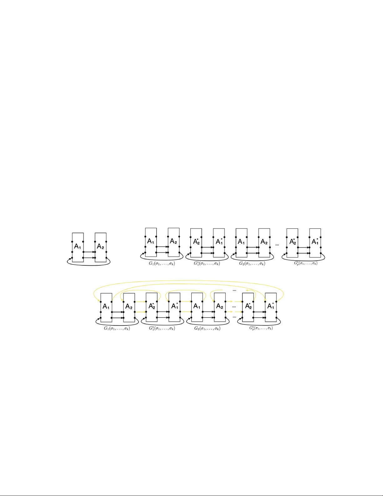
Op erator Norm Bounds for Multi-leg Matrix T ensors and applications to Random Matrix Theory Beno ˆ ıt Collins ∗ and W ang jun Y uan † Marc h 31, 2026 Abstract W e in vestigate the extremal v alues of partial traces of matrix tensors under op erator norm constraints. T o ev aluate these m ulti-linear quan tities, w e develop a comprehensiv e graphical formalism that enco des m ulti-leg partial traces, partial p erm utations, and their momen ts using colored directed graphs. With this graphical framew ork, we establish optimal, sharp b ounds for the partial trace ( T r σ 1 ⊗ . . . ⊗ T r σ k )( A 1 , . . . , A m ) o ver matrices b ounded by ∥ A i ∥ ≤ 1. Sp ecifically , we prov e that this maximum ev aluates exactly to N M ( σ 1 ,...,σ k ) , where N is the dimension and M represen ts the maximal num ber of directed cycles in the asso ciated graph across all p ossible in ternal vertex pairings. W e further derive explicit op erator norm estimates for matrices generated by partial traces of partial p erm utations. Finally , we apply these combinatorial b ounds to m ulti-matrix random matrix theory . By examining mo dels in volving Ginibre ensem bles, we extend concepts of asymptotic freeness to matrix co efficien t algebras, establishing op erator norm estimates that rigorously separate the asymptotic b eha vior of non-crossing and crossing pairings. Mathematics Sub ject Classification 2020 (MSC2020): Primary 15A60; Secondary 15B52, 46M05, 46L54, 47A30, 47C15, 47N30, 60B20. Keyw ords and phrases: T ensor monomials: P artial trace; Op erator norm for tensors. 1 In tro duction The in tegration of random unitary matrices with resp ect to the Haar measure pla ys a fundamen tal role in random matrix theory , op erator algebras, and free probabilit y . A cen tral algebraic to ol for ev aluating these in tegrals is the W eingarten calculus [ 2 , 6 ]. F or t wo m -tuples of matrices A 1 , . . . , A m and B 1 , . . . , B m in M N ( C ), the exp ectation of their ∗ Departmen t of Mathematics, Kyoto Univ ersit y , Japan. Email: collins@math.ky oto-u.ac.jp † Departmen t of Mathematics, Southern Universit y of Science and T echnology , Shenzhen, China. Email: yw ang jun@connect.hku.hk 1 alternating product intert wined with a Haar-distributed unitary matrix U is giv en b y a sum ov er p erm utations: E [T r ( A 1 U B 1 U ∗ · · · A m U B ∗ m )] = X σ,τ ,ρ ∈P ([ m ]) σ τ ρ =(1 ,...,m ) T r σ ( A 1 , . . . , A m )T r τ ( B 1 , . . . , B m )Wg( ρ, N ) , where P ([ m ]) is the set of all p ermutations on [ m ] = { 1 , 2 , . . . , m } , and T r σ ( A 1 , . . . , A m ) is defined as the product o v er the cycles of σ of the traces of the cyclically ordered products of the matrices. This precise algebraic framework has pla y ed a k ey role in establishing profound analytical results, including sharp op erator norm b ounds for non-commutativ e p olynomials [ 3 ] and strong asymptotic freeness [ 1 ]. More recently , there has been a renew ed interest in extending these mo dels to the tensor setting, where the integral is taken ov er U = U 1 ⊗ · · · ⊗ U k , with each U i b eing an indep enden t Haar-distributed random matrix in M N ( C ) [ 5 ]. Suc h multi-fold tensor mo dels arise naturally in v arious con texts, including the sp ectral distribution of large dimensional tensor pro ducts [ 8 ]. In this setting, the integrations yield com binations of fundamental m ulti-linear tensor inv ariants of the form: (T r σ 1 ⊗ . . . ⊗ T r σ k )( A 1 , . . . , A m ) , (1.1) where A 1 , . . . , A m ∈ M N ( C ) ⊗ k . In this pap er, we turn our attention to controlling the extremal v alues of these tensor in v arian ts ( 1.1 ) under the constrain t that the op erator norms of the co efficient matrices satisfy ∥ A i ∥ ≤ 1. If k = 1, the solution to this problem is trivial: the maxim um is ac hieved when A i = I N for all i , yielding exactly N #cycles( σ 1 ) . How ev er, ev aluating these quan tities b ecomes deeply combinatorial and highly non-trivial as soon as the n um b er of legs k ≥ 2. There are at least three primary motiv ations to systematically delve into this op erator norm analysis: 1. Op erator Algebras and F ree Probabilit y: In the t w o-leg case ( k = 2), this precise maximization problem emerged in the study of Hay es’ random matrix approach to the Peterson-Thom conjecture [ 9 ]. While estimates leveraging the complete p ositivity of partial traces allo w one to conclude that the maximum behav es nicely if σ 1 is non-crossing and σ 2 is the full cycle, extending this to general p ermutations σ 1 , σ 2 requires a fundamentally new understanding of matrix tensors. 2. T ensor Models and In v arian t Theory: The theoretical study of matrix tensors has b een significantly dev elop ed in recent years [ 4 , 5 ], but not y et thoroughly in v estigated within an op erator algebraic framework. Because quantities of the form ( 1.1 ) are the fundamental observ ables of matrix tensors in this theory , establishing sharp ev aluations of these multi-leg traces is a vital preliminary step for future asymptotic analysis. 2 3. Quan tum Information Theory: Bounds on these tensor in v arian ts directly capture the presence and limitations of en tanglemen t across m ultiple tensor subsystems [ 4 , 7 ]. Our results demonstrate that while en tanglement effects actively manifest in these maximization problems, they remain quite tame and structurally b ounded, guided b y underlying symmetries and Sc h ur-W eyl dualit y . T o tackle this, w e develop a comprehensiv e graphical calculus that translates the m ultilinear tensor structure into the analysis of colored directed graphs. Throughout this pap er, for the sak e of clarit y , we carefully detail the pro ofs for the t w o-leg case ( k = 2) b efore generalizing to an arbitrary n umber of legs. W e also extend our framework b eyond full p erm utations to arbitrary partial p ermutations, leading to explicit op erator norm estimates for the resulting m ulti-leg matrices. Let us summarize the main results of this pap er. Our analysis relies on encoding the multi-linear tensor structure in to a colored directed graph G σ 1 ,...,σ k . In this graph, eac h matrix A i is represen ted as a “rectangle” with k in-v ertices and k out-v ertices, and the p erm utations σ j define the external directed edges b et w een different rectangles. By in tro ducing auxiliary in ternal edges (referred to as “blue edges”) that pair the in-v ertices and out-vertices within eac h rectangle, we define our fundamen tal combinatorial in v arian t: let M ( σ 1 , . . . , σ k ) denote the maximal num ber of directed cycles in G σ 1 ,...,σ k o v er all p ossible v alid connections of these internal blue edges. Using this graphical formalism, our first main result exactly ev aluates the maximization problem for the scalar partial trace ov er the unit ball of the op erator norm: Theorem (cf. Theorem 2 ) . F or any inte ger k ≥ 1 and p ermutations σ 1 , . . . , σ k ∈ P ([ m ]) , the maximum of the multi-le g p artial tr ac e over matric es b ounde d in op er ator norm is governe d exactly by the cycle structur e of the gr aph: max ∥ A 1 ∥ ,..., ∥ A m ∥≤ 1 | (T r σ 1 ⊗ . . . ⊗ T r σ k ) ( A 1 , . . . , A m ) | = N M ( σ 1 ,...,σ k ) . W e then extend this top ological counting to the case where σ 1 , . . . , σ k are p artial p ermutations . W e denote by P ′ ([ m ]) the set of partial p ermutations on [ m ]. In this regime, the partial trace do es not con tract all indices and consequently outputs a multi-leg matrix Y rather than a scalar. By lifting the graph structure to enco de the momen ts T r (( Y Y ∗ ) p ), w e obtain optimal, sharp estimates on the op erator norm: Theorem (cf. Theorem 3 and Corollary 6 ) . F or any p artial p ermutations σ 1 , . . . , σ k ∈ P ′ ([ m ]) , let Y b e the matrix r esulting fr om the p artial tr ac e evaluation. The op er ator norm of Y satisfies the sharp b ound: max ∥ A 1 ∥ ,..., ∥ A m ∥≤ 1 ∥ Y ∥ = N M ( σ 1 ,...,σ k ) . Finally , we apply these deterministic, com binatorial op erator norm b ounds to multi- matrix random matrix theory . By examining matrices conjugated b y Ginibre ensembles (as a com binatorially tractable proxy for Haar unitaries), we establish operator norm estimates on the co efficien t algebra that rigorously isolate top ological con tributions. 3 Theorem (cf. Theorems 7 and 8 ) . In the c ontext of the matrix c o efficient algebr a sc ale d with differing le g dimensions N d 1 and N d 2 , the p artial tr ac e limits sharply distinguish top olo gic al p airings of the Ginibr e matric es. We establish explicit op er ator norm b ounds demonstr ating that cr ossing (non-planar) p airings ar e suppr esse d c omp ar e d to non-cr ossing (planar) p airings by a factor of O ( N d 2 − d 1 ) when d 2 < d 1 . Organization of the pap er The pap er is organized as follo ws. In Section 2 , we in tro duce the essen tial graphical terminology and construct the directed graphs asso ciated with t wo-leg partial traces, m ultiple legs, and partial p erm utations. Section 3 presen ts our main results, detailing the optimal op erator norm b ounds for partial traces across v arious tensor configurations. In Section 4 and Section 5 , we resp ectively establish the upp er and low er b ounds for the t w o-leg case, whic h culminates in the pro of of Theorem 1 in Section 6 . Section 7 extends these arguments to the m ultiple-leg setting to prov e Theorem 2 . In Section 8 , we establish the matrix estimates for partial permutations b y proving Theorem 3 , while Section 9 con tains the proofs of the asso ciated corollaries. Finally , in Section 10 , w e apply our main theorems to m ulti-matrix random matrix theory , exploring the asymptotic b eha vior of Ginibre ensembles. Ac knowledgemen ts BC was supported b y JSPS Gran t-in-Aid Scientific Researc h (A) no. 25H00593, and Challenging Research (Exploratory) no. 23K17299. WY was supported b y Guangdong Basic and Applied Basic Researc h F oundation (No. 2026A1515030040), and National Natural Science F oundation of China (No. 12501183), and a Gran t of the Departmen t of Science and T echnology of Guangdong Pro vince (No. 2024QN11X161). 2 Graphical notation In order to present our main results, w e need to in tro duce graphical terminology . In this section, w e first introduce the graph corresp onding to the partial trace for the case of 2 legs in Section 2.1 , and then the graph for the m ultiple leg v ersion in Section 2.2 . Then in Section 2.3 , we extend the graphs for partial p ermutations, which plays a k ey role in our pro ofs. Lastly , we construct the graph for the moments of the partial trace of partial p erm utations via its partial graph in Section 2.4 . 2.1 Graph for 2 legs W e start with case k = 2 as a w arm-up. In this man uscript, w e tak e the stance that a go o d understanding of the case with tw o legs will facilitate the statement and the proof of 4 the general case. Therefore, our first goal is to handle the following: for any p erm utations σ 1 , σ 2 ∈ P ([ m ]), w e compute the follo wing partial trace: (T r σ 1 ⊗ T r σ 2 ) ( A 1 , . . . , A m ) (2.1) and find its maxim um among all unitary matrices A 1 , . . . , A m ∈ M N ( C ) ⊗ M N ( C ). W e use a graph with the notation G σ 1 ,σ 2 ( A 1 , . . . , A m ) for the representation of the partial trace ( 2.1 ) . W e use m rectangles for the matrices A 1 , . . . , A m . W e connect the rectangles with directed edges according to the p ermutations σ 1 , σ 2 . F or the p erm utation σ 1 , for all i , we use a green directed edge to connect the rectangles A i and A σ 1 ( i ) with the orien tation from the rectangle A i to the rectangle A σ 1 ( i ) . The vertices of the green edge on the rectangle A i and the rectangle A σ 1 ( i ) are called the green out-vertex and the green in-vertex , resp ectiv ely . W e also call the green edge an out-e dge of A i and an in-e dge of A σ 1 ( i ) . W e use red directed edges to connect rectangles for any p erm utation σ 2 , follo wing the same rule. That is, the red directed edges are from A i to A σ 2 ( i ) . Then, ev ery rectangle has one green in-edge, one green out-edge, one red in-edge, and one red out-edge. Th us, there are four v ertices on ev ery rectangle: the green in-vertex, the green out-vertex, the red in-vertex, and the red out-v ertex. Moreo ver, if w e shrink ev ery rectangle to a point, then the connected comp onent of the red and green directed edges corresp ond to the block of the p erm utation σ 2 and σ 1 , resp ectively . It is obvious that the graph defined ab o ve has m red edges and m green edges. F or simplicity , w e alwa ys dra w the out-v ertices on the righ t of the rectangles, and the in-v ertices on the left of the rectangles. Unless specified otherwise, the quan tities we considered in the sequel do not dep end on the p osition of each rectangle. Without loss of generality , we alw ays list the rectangles A 1 , . . . , A m from left to righ t. Figure 1 b elo w is an example for m = 4, σ 1 = (1 , 2 , 3)(4), and σ 2 = (1 , 2 , 3 , 4). Figure 1: Graph G σ 1 ,σ 2 ( A 1 , . . . , A m ) with m = 4 and σ 1 = (1 , 2 , 3)(4), σ 2 = (1 , 2 , 3 , 4) Next, we in tro duce some auxiliary directed edges for the graph G σ 1 ,σ 2 ( A 1 , . . . , A m ). F or all rectangles, w e use blue directed edges to pair the in-vertices and out-v ertices of the same rectangle. The blue directed edges are arbitrary , with the constrain ts that their orien tations are from the in-vertices to the out-vertices of the same rectangles and that different blue directed edges do not share any common vertices. As every rectangle has tw o in-vertices and t wo out-v ertices, it has tw o blue directed edges. There are tw o differen t p ossibilities for the pair of blue directed edges: the vertices of the blue directed edges ma y ha ve the 5 same color or differen t colors. In the follo wing, all graphs refer to the graphs without blue directed edges unless otherwise sp ecified. Figure 2 is an example of a p ossibilit y of the blue directed edges in Figure 1 . Figure 2: Blue directed edges in graph G σ 1 ,σ 2 ( A 1 , . . . , A m ) with m = 4 and σ 1 = (1 , 2 , 3)(4), σ 2 = (1 , 2 , 3 , 4) W e call G ′ σ 1 ,σ 2 ( A 1 , . . . , A m ) a p artial gr aph if it can b e obtained from G σ 1 ,σ 2 ( A 1 , . . . , A m ) b y removing some red directed edges, green directed edges, and rectangles. The green di- rected edges, red directed edges, and rectangles, whic h are remov ed from G σ 1 ,σ 2 ( A 1 , . . . , A m ) to obtain the partial graph G ′ σ 1 ,σ 2 ( A 1 , . . . , A m ), form a partial graph G ′′ σ 1 ,σ 2 ( A 1 , . . . , A m ). The partial graph G ′′ σ 1 ,σ 2 ( A 1 , . . . , A m ) is called the c omplement of G ′ σ 1 ,σ 2 ( A 1 , . . . , A m ). 2.2 Graph for multiple legs No w w e in tro duce the multiple legs v ersion of the graph. F or permutations σ 1 , . . . , σ k ∈ P ([ m ]), w e can interpret the partial trace ( 1.1 ) as a graph G σ 1 ,...,σ k ( A 1 , . . . , A m ) that is similar to the graph in Section 2.1 . W e sketc h the description b elow. The graph G σ 1 ,...,σ k ( A 1 , . . . , A m ) has m rectangles, A 1 , . . . , A m , whic h represen t the corre- sp onding matrices. W e in tro duce k colors col 1 , . . . , col k corresp onding to the k p erm utations σ 1 , . . . , σ k . F or 1 ≤ j ≤ k , w e connect the m directed edges with the color col j for the p erm utation σ j in the graph G σ 1 ,...,σ k ( A 1 , . . . , A m ) as follo ws. F or 1 ≤ i ≤ m , we connect a directed edge of color col j b et ween A i and A σ j ( i ) with an orien tation from A i to A σ j ( i ) . F or this edge, the v ertex on A i is an out-v ertex, while the vertex on A σ j ( i ) is an in-v ertex. Both v ertices are colored with color col j . Th us, eac h rectangle has k out-v ertices and k in-v ertices, and the k out-v ertices and the k in-v ertices are of color col 1 , . . . , col k , resp ectively . W e provide an example in Figure 3a for the graph G σ 1 ,...,σ k ( A 1 , . . . , A m ). F or practical reasons, we do not represent the colors in the picture. In the graph G σ 1 ,...,σ k ( A 1 , . . . , A m ), we connect the in-vertices and the out-v ertices in each rectangle using k blue directed edges with the orientation from in-v ertices to out-vertices, suc h that the blue directed edges do not hav e an y common v ertices. An example of blue directed edges for the graph G σ 1 ,...,σ k ( A 1 , . . . , A m ) is pro vided in Figure 3b . F or the graph G σ 1 ,...,σ k ( A 1 , . . . , A m ), if w e remov e some directed edges and rectangles, the remaining part G ′ σ 1 ,...,σ k ( A 1 , . . . , A m ) is called a p artial graph of G σ 1 ,...,σ k ( A 1 , . . . , A m ). The 6 (a) Graph G σ 1 ,...,σ 4 ( A 1 , . . . , A 4 ) (b) Graph G σ 1 ,...,σ 4 ( A 1 , . . . , A 4 ) with blue di- rected edges Figure 3: Graph G σ 1 ,...,σ 4 ( A 1 , . . . , A 4 ) with σ 1 = σ 2 = (123)(4) and σ 3 = σ 4 = (1234) directed edges and rectangles that are remo v ed from the graph G σ 1 ,...,σ k ( A 1 , . . . , A m ) when obtaining the partial graph G ′ σ 1 ,...,σ k ( A 1 , . . . , A m ) form a partial graph G ′′ σ 1 ,...,σ k ( A 1 , . . . , A m ). The partial graph G ′′ σ 1 ,...,σ k ( A 1 , . . . , A m ) is called the c omplement of G ′ σ 1 ,...,σ k ( A 1 , . . . , A m ). 2.3 Graphs for partial p erm utations Recall that Y is the matrix in tro duced in Section 1 . In order to provide a graphical expla- nation for Y , we need to extend the graph defined previously for the partial p erm utations. F or partial p ermutations σ 1 , . . . , σ k ∈ P ′ ([ m ]), we interpret the matrix Y of the partial trace given in ( 1.1 ) as a graph G σ 1 ,...,σ k ( A 1 , . . . , A m ) with an idea similar to that of Section 2.2 . W e sketc h the description in the following. The graph G σ 1 ,...,σ k ( A 1 , . . . , A m ) has m rectangles, A 1 , . . . , A m , which represen t the corresp onding matrices. F or all 1 ≤ j ≤ k , we connect the directed edges with the color col j according to each partial p erm utation σ j . F or 1 ≤ j ≤ k , for the partial permutation σ j , the directed edges are from A i to A σ j ( i ) for all i ∈ D ( σ j ). F or the edge from A i to A σ j ( i ) , the vertex on A i is an out-vertex with color col j , while the v ertex on A σ j ( i ) is an in-vertex with color col j . Note that when i / ∈ D ( σ j ), the partial permutation σ j do es not pro vide an out-edge for rectangle A i . In this case, we add an out-vertex with color col j on A i . Similarly , if i is not in the image of σ j , then σ j do es not provide an in-edge for rectangle A i . W e also add an in-v ertex with color col j on A i . W e call the in-vertices and out-vertices w e added in this w ay op en in-v ertices and op en out-v ertices, resp ectively . Th us, in the graph G σ 1 ,...,σ k ( A 1 , . . . , A m ), eac h rectangle has k in-v ertices and k out- v ertices, and eac h out-v ertex and in-v ertex is of differen t colors from col 1 , . . . , col k . The n um b ers of op en in-vertices and op en out-v ertices are the same, which is P k j =1 ( m − D ( σ j )). Moreo v er, the num b er of directed edges in the graph G σ 1 ,...,σ k ( A 1 , . . . , A m ) is P k j =1 D ( σ j ). W e pro vide an example in Figure 4a for the graph G σ 1 ,...,σ k ( A 1 , . . . , A m ). In the graph G σ 1 ,...,σ k ( A 1 , . . . , A m ), we can connect the in-v ertices and the out-v ertices in the same rectangle using k blue directed edges whose orien tation is from in-v ertices to out-vertices, such that the blue directed edges do not hav e an y common v ertices. An example of blue directed edges for the graph G σ 1 ,...,σ k ( A 1 , . . . , A m ) is pro vided in Figure 4b . 7 (a) Graph G σ 1 ,σ 2 ,σ 3 ( A 1 , . . . , A 3 ) (b) Graph G σ 1 ,σ 2 ,σ 3 ( A 1 , . . . , A 3 ) with blue di- rected edges Figure 4: k = m = 3, graph G σ 1 ,σ 2 ,σ 3 ( A 1 , . . . , A 3 ), σ 2 = σ 3 = (123) and σ 1 (1) = 2 , σ 1 (2) = 3 Let us make the follo wing remarks ab out partial graphs: Remark 1. A gr aph G σ 1 ,...,σ k ( A 1 , . . . , A m ) for p artial p ermutations σ 1 , . . . , σ k ∈ P ′ ([ m ]) c an b e viewe d as a p artial gr aph of some gr aph G σ ′ 1 ,...,σ ′ k ( A 1 , . . . , A m ) for some p ermutations σ ′ 1 , . . . , σ ′ k . However, for a gr aph G σ ′ 1 ,...,σ ′ k ( A 1 , . . . , A m ) with some p ermutations σ ′ 1 , . . . , σ ′ k ∈ P ([ m ]) , its p artial gr aph G ′ σ ′ 1 ,...,σ ′ k ( A 1 , . . . , A m ) may not b e a gr aph of some p artial p ermutations. Lastly , note that the properties of graphs in whic h w e are in terested do not dep end on the v alue of A 1 , . . . , A m . Hence, the graph can also b e understo o d as a map on the space of matrices. Remark 2. F or k , m ∈ N , for p artial p ermutations σ 1 , . . . , σ k ∈ P ′ ([ m ]) , the gr aph G σ 1 ,...,σ k ( A 1 , . . . , A m ) is a matrix that b elongs to M N m − D ( σ 1 ) ( C ) ⊗ . . . ⊗ M N m − D ( σ k ) ( C ) . This c orr esp ondenc e induc es a multi-line ar mapping G σ 1 ,...,σ k :  ( M N ( C )) ⊗ k  m − → M N m − D ( σ 1 ) ( C ) ⊗ . . . ⊗ M N m − D ( σ k ) ( C ) . In the se quel, we abuse the notation G σ 1 ,...,σ k ( A 1 , . . . , A m ) and G σ 1 ,...,σ k if we do not emphasize the matric es A 1 , . . . , A m . 2.4 Graphs for moments As we deal with the moments of Y , we in tro duce the graph G ( p ) σ 1 ,...,σ k ( A 1 , . . . , A m ) for the momen t T r (( Y Y ∗ ) p ) for an y p ∈ N , we need to introduce the graph for the matrix Y ∗ . F or a partial p ermutation σ ∈ P ′ ([ m ]), w e define σ − 1 the in verse of σ in the sense that σ − 1 is also a partial p ermutation from the image of σ to D ( σ ), so that σ − 1 σ is the iden tity of D ( σ ). Ob viously , σ − 1 is well-defined. With the help of this notation, we hav e Y ∗ =  T r σ − 1 1 ⊗ . . . ⊗ T r σ − 1 k  ( A ∗ m , . . . , A ∗ 1 ) . (2.2) W e in tro duce the graph G ∗ σ 1 ,...,σ k ( A ∗ 1 , . . . , A ∗ m ) for the matrix Y ∗ in a w ay similar to the graph for Y ab o ve. W e use rectangles A ∗ 1 , . . . , A ∗ m for the matrices and connect the rectangles 8 with directed edges according to the partial p ermutations σ 1 , . . . , σ k . F or 1 ≤ j ≤ k , for i ∈ D ( σ j ), w e connect a directed edge with color col j from the rectangle A ∗ σ j ( i ) to the rectangle A ∗ i . F or 1 ≤ j ≤ k , if i / ∈ D ( σ − 1 j ), w e add an out-v ertex with color col j on A ∗ i . W e also add an in-v ertex with color col j on A ∗ i if i / ∈ D ( σ j ). W e can pair the in-vertices and out-vertices of the same rectangle with blue directed edges. The orientation is alwa ys from in-vertices to out-vertices, and different blue directed edges do not share an y common v ertices. F or simplicity , for the graph G ∗ σ 1 ,...,σ k ( A ∗ 1 , . . . , A ∗ m ), we alwa ys dra w the in-v ertices on the left of the rectangles and the out-v ertices on the righ t of the rectangles. W e also list the rectangles from righ t to left in the order A ∗ 1 , . . . , A ∗ m without loss of generalit y , since the quantities we consider do not dep end on the p ositions of the rectangles. An example of the graph G ∗ σ 1 ,...,σ k ( A ∗ 1 , . . . , A ∗ m ) is provided in Figure 5 . (a) Graph G ∗ σ 1 ,σ 2 ,σ 3 ( A ∗ 1 , A ∗ 2 , A ∗ 3 ) (b) Graph G ∗ σ 1 ,σ 2 ,σ 3 ( A ∗ 1 , A ∗ 2 , A ∗ 3 ) with blue di- rected edges Figure 5: k = m = 3, graph G ∗ σ 1 ,σ 2 ,σ 3 ( A ∗ 1 , A ∗ 2 , A ∗ 3 ) with σ 2 = σ 3 = (123) and σ 1 (1) = 2 , σ 1 (2) = 3 Note that the in-v ertex with color col j on the rectangle A i in the graph G σ 1 ,...,σ k ( A 1 , . . . , A m ) is op en if and only if the out-vertex of the same color on the rectangle A ∗ i in the graph G ∗ σ 1 ,...,σ k ( A ∗ 1 , . . . , A ∗ m ) is op en. Similarly , the out-vertex with color col j on the rectangle A i on the graph G σ 1 ,...,σ k ( A 1 , . . . , A m ) is op en if and only if the in-vertex of the same color on the rectangle A ∗ i on the graph G ∗ σ 1 ,...,σ k ( A ∗ 1 , . . . , A ∗ m ) is op en. Moreo v er, the connection of the blue directed edges in the graph G σ 1 ,...,σ k ( A 1 , . . . , A m ) can bijectively correspond to the connection of the blue directed edges in the graph G ∗ σ 1 ,...,σ k ( A ∗ 1 , . . . , A ∗ m ) in the follo wing wa y . F or all 1 ≤ i ≤ m , if a blue directed edge in rectangle A i in the graph G σ 1 ,...,σ k ( A 1 , . . . , A m ) connects the in-vertex of color col j 1 with the out-vertex of color col j 2 , then w e connect the in-vertex of color col j 2 and the out-v ertex of color col j 1 in rectangle A ∗ i in the graph G ∗ σ 1 ,...,σ k ( A ∗ 1 , . . . , A ∗ m ) with a blue directed edge. The orientation of the blue directed edges is alwa ys from in-vertices to out-v ertices. W e refer to Figures 4b and 5b for an example of the corresp ondence of the blue directed edges in G σ 1 ,...,σ k ( A 1 , . . . , A m ) and G ∗ σ 1 ,...,σ k ( A ∗ 1 , . . . , A ∗ m ). Secondly , w e introduce the graph for the moment T r (( Y Y ∗ ) p ) for p ∈ N . Recall the graphs G σ 1 ,...,σ k ( A 1 , . . . , A m ) and G ∗ σ 1 ,...,σ k ( A ∗ 1 , . . . , A ∗ m ) for Y and Y ∗ , resp ectively . W e dupli- cate the graph G σ 1 ,...,σ k ( A 1 , . . . , A m ) for p copies with the notations r G σ 1 ,...,σ k ( A 1 , . . . , A m ), where 1 ≤ r ≤ p . W e also duplicate the graph G ∗ σ 1 ,...,σ k ( A ∗ 1 , . . . , A ∗ m ) for p copies, with the notations r G ∗ σ 1 ,...,σ k ( A ∗ 1 , . . . , A ∗ m ) for 1 ≤ r ≤ p . The graph G ( p ) σ 1 ,...,σ k ( A 1 , . . . , A m ) consists 9 of the graphs r G σ 1 ,...,σ k ( A 1 , . . . , A m ) and r G ∗ σ 1 ,...,σ k ( A ∗ 1 , . . . , A ∗ m ) for 1 ≤ r ≤ p . Next, w e in tro duce the directed edges in G ( p ) σ 1 ,...,σ k ( A 1 , . . . , A m ) that connect differen t copies of r G σ 1 ,...,σ k ( A 1 , . . . , A m ) and r G ∗ σ 1 ,...,σ k ( A ∗ 1 , . . . , A ∗ m ). F or an y 1 ≤ r ≤ p , in the graph r G σ 1 ,...,σ k ( A 1 , . . . , A m ), for an y open out-v ertex on the rectangle A i with color col j for some 1 ≤ i ≤ m and 1 ≤ j ≤ k , w e connect it with the open in-v ertex of color col j on the rectangle A ∗ i in the graph r G ∗ σ 1 ,...,σ k ( A ∗ 1 , . . . , A ∗ m ) using a yel low directed edge. The orientation of this y ello w directed edge is from the out-v ertex to the in-v ertex. Similarly , for any 1 ≤ r ≤ p , in the graph r G ∗ σ 1 ,...,σ k ( A ∗ 1 , . . . , A ∗ m ), for any op en out-vertex on the rectangle A ∗ i with color col j for some 1 ≤ i ≤ m and 1 ≤ j ≤ k , w e connect it with the open in-vertex of color col j on the rectangle A i in the graph r +1 G σ 1 ,...,σ k ( A 1 , . . . , A m ) using a yel low directed edge whose orien tation is from the out-v ertex to the in-vertex. Here, w e use the con v ention p +1 G σ 1 ,...,σ k ( A 1 , . . . , A m ) = 1 G σ 1 ,...,σ k ( A 1 , . . . , A m ). W e pro vide an example in Figure 6 for the graph G ( p ) σ 1 ,...,σ k ( A 1 , . . . , A m ) with k = 3 , m = 2. Figure 6a is the graph G σ 1 ,...,σ k ( A 1 , . . . , A m ), and Figure 6b is the graph that consists of the duplications of G σ 1 ,...,σ k ( A 1 , . . . , A m ) and G ∗ σ 1 ,...,σ k ( A ∗ 1 , . . . , A ∗ m ). Figure 6c is the corresp onding graph G ( p ) σ 1 ,...,σ k ( A 1 , . . . , A m ). (a) Graph G σ 1 ,...,σ 3 ( A 1 , A 2 ) (b) Graphs 1 G ( σ 1 , . . . , σ 3 )( A 1 , A 2 ), . . . , p G ∗ σ 1 ,...,σ 3 ( A ∗ 1 , A ∗ 2 ) (c) Graph G ( p ) σ 1 ,...,σ 3 ( A 1 , A 2 ) Figure 6: k = 3 , m = 2, graph G ( p ) σ 1 ,...,σ k ( A 1 , . . . , A m ) with σ 1 = ∅ , σ 2 (1) = 2 and σ 3 = (12) In particular, in the graph G ( p ) σ 1 ,...,σ k ( A 1 , . . . , A m ), the n umber of yello w directed edges is 2 p P k j =1 ( m − D ( σ j )) and the n umber of other edges is 2 p P k j =1 D ( σ j ). Let us point out that the graph G ( p ) σ 1 ,...,σ k ( A 1 , . . . , A m ) is a graph of a t yp e introduced in Section 2.2 , if we replace the color of the y ellow directed edges with the color of their v ertices. Hence, w e can pair the in-vertices with the out-vertices of the same rectangles in the graph G ( p ) σ 1 ,...,σ k ( A 1 , . . . , A m ) using blue directed edges, as in Section 2.2 . 10 3 Main results In this pap er, we obtain a result irresp ectiv e of the num b er of legs in the tensor mo del. Ho w ever, for the sak e of clarity , w e choose to “w arm up” with the tw o leg case, whose pro of w e give in detail, b efore tackling the general k -legs mo del. 3.1 P artial trace with 2 legs Our first result is an optimal bound for the maxim um of the partial trace under op erator norm conditions for the A i ’s. Theorem 1. F or m, N ∈ N , for any p ermutations σ 1 , σ 2 ∈ P ([ m ]) , we denote by M ( σ 1 , σ 2 ) the maximal numb er of dir e cte d cycles in the c orr esp onding gr aph G σ 1 ,σ 2 , wher e the maximum is taken over al l p ossibilities of blue dir e cte d e dges. Then we have max A 1 ,...,A m | (T r σ 1 ⊗ T r σ 2 ) ( A 1 , . . . , A m ) | = N M ( σ 1 ,σ 2 ) , wher e the maximum is taken among al l unitary matric es A 1 , . . . , A m ∈ M N ( C ) ⊗ M N ( C ) . Since an y matrix of op erator norm less than 1 is a con v ex combination of unitary matrices, we obtain the follo wing corollary: Corollary 1. F or m, N ∈ N , for any p ermutations σ 1 , σ 2 ∈ P ([ m ]) , for any A 1 , . . . , A m ∈ M N ( C ) ⊗ M N ( C ) , we have max ∥ A 1 ∥ ,..., ∥ A m ∥≤ 1 | (T r σ 1 ⊗ T r σ 2 ) ( A 1 , . . . , A m ) | = N M ( σ 1 ,σ 2 ) . Since M ( σ 1 , σ 2 ) can b e difficult to c haracterize, w e presen t an estimate of the n umber of directed cycles in the graph G ( σ 1 , σ 2 ) that is related only to the permutations. F or an y p erm utation σ ∈ P ([ m ]), w e denote by R ( σ ) the n um b er of i ∈ [ m ] such that σ ( i ) ≤ i . This index i corresp onds to the edge going from righ t to left. More precisely , in the graph G ( σ 1 , σ 2 ), w e call the green directed edge from A i to A σ 1 ( i ) (resp. the red directed edge from A i to A σ 2 ( i ) ) a b ackwar d directed edge if i ≥ σ 1 ( i ) (resp. i ≥ σ 2 ( i )). F rom the fact that ev ery directed cycle must con tain at least one bac kw ard directed edge, one can immediately deduce the following corollary . Corollary 2. F or m, N ∈ N , for any p ermutations σ 1 , σ 2 ∈ P ([ m ]) , for any A 1 , . . . , A m ∈ M N ( C ) ⊗ M N ( C ) , we have max ∥ A 1 ∥ ,..., ∥ A m ∥≤ 1 | (T r σ 1 ⊗ T r σ 2 ) ( A 1 , . . . , A m ) | ≤ N R ( σ 1 )+ R ( σ 2 ) . Remark 3. Firstly, we would like to mention that the numb er of b ackwar d dir e cte d e dges in G ( σ 1 , σ 2 ) is a quantity that dep ends on the p ositions of the r e ctangles. Mor e pr e cisely, for any θ ∈ P ([ m ]) , we have max A 1 ,...,A m (T r σ 1 ⊗ T r σ 2 ) ( A 1 , . . . , A m ) = max A 1 ,...,A m (T r θσ 1 θ − 1 ⊗ T r θσ 2 θ − 1 )  A θ (1) , . . . , A θ ( m )  . 11 Henc e, max A 1 ,...,A m | (T r σ 1 ⊗ T r σ 2 ) ( A 1 , . . . , A m ) | ≤ N R ( θ σ 1 θ − 1 )+ R ( θ σ 2 θ − 1 ) . Se c ond ly, we would like to p oint out that the upp er b ound in Cor ol lary 2 is not optimal. We c onsider the example wher e σ 1 = (164253) and σ 2 = (123456) . In this c ase, R ( σ 1 ) = 4 as 6 → 4 → 2 and 5 → 3 → 1 , while R ( σ 2 ) = 1 . Thus, the upp er b ound in Cor ol lary 2 is N 5 . F or the example ab ove, if we r e-lab el by 1 ↔ 5 and 2 ↔ 6 , we have θ σ 1 θ − 1 = (524613) and θ σ 2 θ − 1 = (563412) . In this c ase, we have R ( θ σ 1 θ − 1 ) = 2 and R ( θ σ 2 θ − 1 ) = 2 . Thus, the upp er b ound ab ove b e c omes N 4 . 3.2 P artial trace with m ultiple legs Let k ∈ N b e the num b er of legs and N ∈ N b e the dimension of each leg. The multi-leg v ersion of Theorem 1 is as follows: Theorem 2. F or any k , N ∈ N , for any p ermutations σ 1 , . . . , σ k ∈ P ([ m ]) , we denote by M ( σ 1 , . . . , σ k ) the maximal numb er of dir e cte d cycles in the gr aph G σ 1 ,...,σ k among al l p ossible c onne ctions of blue dir e cte d e dges. Then for any m ∈ N and matric es A 1 , . . . , A m ∈ M N ( C ) ⊗ k , we have max ∥ A 1 ∥ ,..., ∥ A m ∥≤ 1 | (T r σ 1 ⊗ . . . ⊗ T r σ k ) ( A 1 , . . . , A m ) | = N M ( σ 1 ,...,σ k ) . With the help of Theorem 2 , we can handle the case of t w o legs of different dimensions. Corollary 3. L et m, N , a, b ∈ N , and let σ, τ ∈ P ([ m ]) b e any p ermutations. We denote by M ( σ, τ ; a, b ) the maximal numb er of dir e cte d cycles in the c orr esp onding gr aph G σ,...,σ ,τ ,...,τ , wher e σ r ep e ats a times and τ r ep e ats b times, and wher e the maximum is taken over al l p ossibilities of blue dir e cte d e dges. Then for any A 1 , . . . , A m ∈ M N a ( C ) ⊗ M N b ( C ) , we have max ∥ A 1 ∥ ,..., ∥ A m ∥≤ 1 | (T r σ ⊗ T r τ ) ( A 1 , . . . , A m ) | = N M ( σ,τ ; a,b ) , Indeed, we also allow for the case of multiple legs having differen t dimensions for eac h leg. Corollary 4. L et m, N , k ∈ N , a 1 , . . . , a k ∈ N , and let σ 1 , . . . , σ k ∈ P ([ m ]) b e any p ermu- tations. We denote by M ( σ 1 , . . . , σ k ; a 1 , . . . , a k ) the maximal numb er of dir e cte d cycles in the c orr esp onding gr aph G σ 1 ,...,σ 1 ,...,σ k ,...,σ k , wher e σ j r ep e ats a j times for 1 ≤ j ≤ k , and wher e the maximum is taken over al l p ossibilities of blue dir e cte d e dges. Then for any A 1 , . . . , A m ∈ M N a 1 ( C ) ⊗ . . . ⊗ M N a k ( C ) , we have max ∥ A 1 ∥ ,..., ∥ A m ∥≤ 1 | (T r σ 1 ⊗ . . . ⊗ T r σ k ) ( A 1 , . . . , A m ) | = N M ( σ 1 ,...,σ k ; a 1 ,...,a k ) , 12 No w we turn to a sp ecial setting, where σ 1 = σ ∈ P ([ m ]) is an arbitrary p ermutation, and σ 2 = . . . = σ k = γ , where γ = (123 . . . m ) ∈ P . W e consider k to b e large. In this setting, the upp er b ound in the m ultiple leg v ersion of Corollary 2 is optimal. Corollary 5. L et m, k , N ∈ N . F or any p ermutation σ ∈ P ([ m ]) , for any matric es A 1 , . . . , A m ∈ M N ( C ) ⊗ k , for any k ≥ m + 1 , we have max ∥ A 1 ∥ ,..., ∥ A m ∥≤ 1 | (T r σ ⊗ T r γ ⊗ . . . ⊗ T r γ ) ( A 1 , . . . , A m ) | = N R ( σ )+ k − 1 . Remark 4. The c ondition k ≥ m + 1 c an b e we akene d as fol lows. F or i ∈ [ m − 1] such that σ ( i ) < i , we define the set I i = { u ∈ N : σ ( i ) < u ≤ i } . We intr o duc e the op er ation such that if I i ∩ I j = ∅ , we c an r eplac e b oth I i and I j by I i ∪ I j . We c ontinue this op er ation until no mor e op er ations c an b e applie d. L et K b e the numb er of r emaining sets. Then c ondition k ≥ m + 1 c an b e impr ove d k ≥ K + 1 . We do not know whether this impr ovement is optimal. In R emark 6 we explain how to make this impr ovement. Remark 5. Note that when k is lar ge, any p ermutation θ acting by c onjugation on γ wil l incr e ase R ( γ ) . By Cor ol lary 2 , sinc e we have k − 1 c opies of γ , this phenomenon incr e ases as k incr e ases. 3.3 Matrix of partial trace for partial p erm utations Let m, k , N ∈ N , for any partial p ermutations σ 1 , . . . , σ k ∈ P ′ ([ m ]), and for matrices A 1 , . . . , A m ∈ M N ( C ) ⊗ k , consider the follo wing matrix Y = (T r σ 1 ⊗ T r σ 2 ⊗ . . . ⊗ T r σ k ) ( A 1 , . . . , A m ) , whic h b elongs to M N m −| D ( σ 1 ) | ( C ) ⊗ . . . ⊗ M N m −| D ( σ k ) | ( C ). W e ha ve the following estimate of Y . Theorem 3. L et m, k , N ∈ N . F or p artial p ermutations σ 1 , . . . , σ k ∈ P ′ ([ m ]) , we denote by M ( σ 1 , . . . , σ k ) the maximum numb er of dir e cte d cycles in the c orr esp onding gr aph G σ 1 ,...,σ k . Then for any matric es A 1 , . . . , A m ∈ M N ( C ) ⊗ k , we have max ∥ A 1 ∥ ,..., ∥ A m ∥≤ 1 | T r (( Y Y ∗ ) p ) | = N 2 pM ( σ 1 ,...,σ k )+ P k j =1 ( m − D ( σ j )) , ∀ p ∈ N . (3.1) Mor e over, the matric es A 1 , . . . , A m , which attain the maximum in ( 3.1 ) , c an b e chosen not to dep end on p . Cho osing p ∈ N to b e large enough, we obtain the follo wing estimate on the op erator norm of Y . Corollary 6. L et the c onditions of The or em 3 hold. Then we have max ∥ A 1 ∥ ,..., ∥ A m ∥≤ 1 ∥ Y ∥ = N M ( σ 1 ,...,σ k ) . 13 4 Upp er b ound in the 2 legs case In this section, w e establish the upp er bound for the partial trace ( 2.1 ). 4.1 Upp er b ound for partial trace F or an y permutations σ 1 , σ 2 ∈ P ([ m ]), w e consider the corresp onding graph G σ 1 ,σ 2 ( A 1 , . . . , A m ) with rectangles A 1 , . . . , A m defined in Section 2.1 . W e call the partial graph G ′ σ 1 ,σ 2 ( A 1 , . . . , A m ) of G σ 1 ,σ 2 ( A 1 , . . . , A m ) a simple partial graph if for all possibilities of the blue directed edges in all the rectangles of G ′ σ 1 ,σ 2 ( A 1 , . . . , A m ), there is no directed cycle in G ′ σ 1 ,σ 2 ( A 1 , . . . , A m ). If G ′ σ 1 ,σ 2 ( A 1 , . . . , A m ) is a simple partial graph of G σ 1 ,σ 2 ( A 1 , . . . , A m ) with m rectangles, then w e call G ′ σ 1 ,σ 2 ( A 1 , . . . , A m ) a ful l simple partial graph of G σ 1 ,σ 2 ( A 1 , . . . , A m ). W e also consider the complement partial graph G ′′ σ 1 ,σ 2 ( A 1 , . . . , A m ) of the simple partial graph G ′ σ 1 ,σ 2 ( A 1 , . . . , A m ) in G σ 1 ,σ 2 ( A 1 , . . . , A m ). Then G ′′ σ 1 ,σ 2 ( A 1 , . . . , A m ) is a graph that consists of only green directed edges and red directed edges, if G ′ σ 1 ,σ 2 ( A 1 , . . . , A m ) is a full simple partial graph of G σ 1 ,σ 2 ( A 1 , . . . , A m ). In this case, we denote b y R G ′ σ 1 ,σ 2 the num b er of edges in the complement partial graph G ′′ σ 1 ,σ 2 ( A 1 , . . . , A m ). The follo wing result is the upp er b ound for the partial trace ( 2.1 ) , and is the main result in this section. Theorem 4. F or any p ermutations σ 1 , σ 2 ∈ P ([ m ]) , for any N ∈ N , we have max A 1 ,...,A m | (T r σ 1 ⊗ T r σ 2 ) ( A 1 , . . . , A m ) | ≤ min G ′ σ 1 ,σ 2 N R G ′ σ 1 ,σ 2 . Her e, max A 1 ,...,A m is taken over al l unitary matric es A 1 , . . . , A m ∈ M N ( C ) ⊗ M N ( C ) , and min G ′ σ 1 ,σ 2 is taken over al l ful l simple p artial gr aphs G ′ σ 1 ,σ 2 of G σ 1 ,σ 2 . 4.2 Pro of of Theorem 4 W e can in terpret the graph G σ 1 ,σ 2 ( A 1 , . . . , A m ) of the partial trace ( 2.1 ) as the inner pro duct of a partial graph G ′ σ 1 ,σ 2 ( A 1 , . . . , A m ) of G σ 1 ,σ 2 ( A 1 , . . . , A m ) and its complemen t partial graph G ′′ σ 1 ,σ 2 ( A 1 , . . . , A m ). W e take the graph in Figure 1 as an example; it can be in terpreted as the inner pro duct of t wo partial graphs given in Figure 7 . F or example, if G σ 1 ,σ 2 ( A 1 , . . . , A m ) is a n umber, i.e., if σ 1 , σ 2 are p ermutations, then w e hav e G σ 1 ,σ 2 ( A 1 , . . . , A m ) = T r ( G ′ σ 1 ,σ 2 ( A 1 , . . . , A m ) · G ′′ σ 1 ,σ 2 ( A 1 , . . . , A m )). If σ 1 , σ 2 are not p erm utations but partial p ermutations, G σ 1 ,σ 2 ( A 1 , . . . , A m ) is no longer a n umber, but a matrix. In this case to o, a counterpart statemen t holds, ho w ever, the trace (or scalar pro duct) has to b e replaced by a partial trace. Next, we introduce the follo wing prop erties of simple partial graphs, which play a k ey role in computing the inner pro duct. Lemma 1. F or any m ∈ N , for any p ermutations σ 1 , σ 2 ∈ P ([ m ]) , we c onsider the gr aph G σ 1 ,σ 2 . L et H b e a simple p artial gr aph of the gr aph G σ 1 ,σ 2 . F or any p artial gr aph H ′ of H , it is a simple p artial gr aph of the gr aph G σ 1 ,σ 2 . 14 Figure 7: Inner pro duct of Figure 1 The pro of of this lemma is directly from the definition of simple partial graphs and is omitted. Lemma 2. F or any m ∈ N , for any p ermutations σ 1 , σ 2 ∈ P ([ m ]) , we c onsider the gr aph G σ 1 ,σ 2 . L et H b e a simple p artial gr aph of the gr aph G σ 1 ,σ 2 . Then in H , ther e exists a r e ctangle A i , such that either A i do es not have out-e dges or A i do es not have in-e dges. Pr o of. W e pro ve the lemma by con tradiction. Assume that all rectangles in H ha v e in-edges and out-edges. W e will connect the blue directed edges in the rectangles to construct a directed cycle in the follo wing wa y . If there is a lo op in H , then we connect the in-vertex and the out-v ertex of this out-edge with a blue directed edge to form a directed cycle. In the following, we only consider the case where there is no lo op in H . W e can start with a rectangle A i 1 for i 1 ∈ [ m ]. By assumption, the rectangle A i 1 has an out-edge. W e denote b y A i 2 the successor of A i 1 with resp ect to this out-edge, where i 2 ∈ [ m ] and i 2  = i 1 . Since the rectangle A i 2 also has an out-edge, we denote by A i 3 the successor of A i 2 with resp ect to this out-edge, where i 3 ∈ [ m ] and i 3  = i 2 . W e connect the in-v ertex of A i 2 of the in-edge from A i 1 to A i 2 with the out-v ertex of A i 2 of the out-edge from A i 2 to A i 3 . W e contin ue this pro cedure to obtain a sequence of indices i 1  = i 2  = . . . , suc h that there is a directed edge from rectangle A i r − 1 to rectangle A i r , and a directed edge from rectangle A i r to rectangle A i r +1 , and a blue directed edge in rectangle A i r connects the in-vertex of this in-edge with the out-vertex of this out-edge. W e pro vide an example of the blue directed edges in Figure 8 . Figure 8: Blue directed edges for cycles As the n um b er of rectangles in the graph H is finite, the sequence of indices of the directed path i 1  = i 2  = . . . con tains only finitely many differen t n umbers. Hence, there exist in tegers t < s , such that i t = i s , and i t , i t +1 , . . . , i s − 1 are distinct. Then we hav e a directed cycle A i t → A i t +1 → . . . → A i s = A i t . 15 F or the simple partial graph of H , the existence of directed cycles under our choice of blue directed edges is a con tradiction. This concludes the pro of. In order to establish the upp er bound, w e need the following lemmas to compute the norm of the simple partial graph. Lemma 3. F or any m ∈ N , for any p ermutations σ 1 , σ 2 ∈ P ([ m ]) , we c onsider the gr aph G σ 1 ,σ 2 . L et H b e a simple p artial gr aph of gr aph G σ 1 ,σ 2 . L et k b e the numb er of r e ctangles in the gr aph H , r b e the numb er of gr e en dir e cte d e dges in H , and s b e the numb er of r e d dir e cte d e dges in H . Then we have ∥ H ∥ 2 2 = N 2 k − r − s . Pr o of. W e prov e this b y induction on k . W e start with the case k = 1. Note that a simple partial graph with only one rectangle m ust b e a rectangle without edges. Th us, the graph of H consists of one rectangle with no edges. In this case, w e hav e k = 1 , r = s = 0. See Figure 9a . The quantit y ∥ H ∥ 2 2 is represen ted in Figure 9b . Noting that A ∗ 1 A 1 = I N ⊗ I N , we ha v e ∥ H ∥ 2 2 = T r ( A 1 A ∗ 1 ) = N 2 . (a) Graph of H (b) Graph interpretation of ∥ H ∥ 2 2 Figure 9: Case k = 1 Next, w e assume that the conclusion holds for the case k − 1. That is, for an y 1 ≤ r, s ≤ k − 1, for an y simple graph H ′ that has k − 1 rectangles with r green directed edges and s red directed edges, the conclusion holds. No w we consider the graph H with k rectangles A 1 , . . . , A k . Noting that H is a simple partial graph of G σ 1 ,σ 2 , by Lemma 2 , there exists a rectangle whic h either do es not ha ve out-edges or do es not ha ve in-edges. Without loss of generality , w e assume that the rectangle A 1 do es not hav e any in-edges. W e consider the num b er of out-edges of A 1 . W e hav e the follo wing four cases. Case 1. There is neither a green out-edge nor a red out-edge on rectangle A 1 ; therefore, rectangle A 1 do es not ha ve an y edges. See Figure 10a for the graph H and Figure 10b 16 (a) Graph of H (b) ∥ H ∥ 2 2 (c) ∥ H ′ ∥ 2 2 (d) Graph of H ′ Figure 10: Case 1 for ∥ H ∥ 2 2 . W e in tro duce a partial graph H ′ whic h is obtained from H b y remo ving the rectangle A 1 . See Figure 10d for the graph H ′ and Figure 10c for ∥ H ′ ∥ 2 2 . Noting that A ∗ 1 A 1 = I N ⊗ I N , we hav e ∥ H ∥ 2 2 = T r ( A ∗ 1 A 1 ) ∥ H ′ ∥ 2 2 = N 2 ∥ H ′ ∥ 2 2 . (4.1) Moreo v er, according to Lemma 1 , H ′ is also a simple partial graph of G σ 1 ,σ 2 . The n umber of rectangles on the graph H ′ is k − 1, while the num b ers of green edges and red edges are r and s , resp ectively . Th us, b y the induction h yp othesis, w e hav e ∥ H ′ ∥ 2 2 = N 2( k − 1) − r − s . The pro of is concluded b y substituting this iden tity in to ( 4.1 ). Case 2. There is no green out-edge, but one red out-edge on rectangle A 1 . W e denote b y A i the successor of A 1 with resp ect to this red out-edge. See Figure 11a for the graph H , and Figure 11b for ∥ H ∥ 2 2 . W e in tro duce a partial graph H ′ that is obtained from H b y remo ving the rectangle A 1 and the red out-edge asso ciated with A 1 . See Figure 11d for the graph H ′ and Figure 11c for ∥ H ′ ∥ 2 2 . (a) Graph of H (b) ∥ H ∥ 2 2 (c) ∥ H ′ ∥ 2 2 (d) Graph of H ′ Figure 11: Case 2 Since A ∗ 1 A 1 = I N ⊗ I N , we hav e ∥ H ∥ 2 2 = T r ( I N ) ∥ H ′ ∥ 2 2 = N ∥ H ′ ∥ 2 2 . (4.2) 17 Moreo v er, according to Lemma 1 , H ′ is also a simple partial graph of G σ 1 ,σ 2 . The n um b er of rectangles in the partial graph H ′ is k − 1, and the n umbers of green edges and red edges are r and s − 1, resp ectiv ely . Th us, by the induction hypothesis, we ha v e ∥ H ′ ∥ 2 2 = N 2( k − 1) − r − ( s − 1) . The pro of is concluded b y substituting this iden tity in to ( 4.2 ). Case 3. There is one green out-edge but no red out-edge on rectangle A 1 . This case is similar to Case 2, and details are omitted. Case 4. There is one green out-edge and one red out-edge on rectangle A 1 . See Figure 12a for the graph H and Figure 12b for ∥ H ∥ 2 2 . Let A i and A j b e the successors of A 1 with resp ect to the red out-edge and the green out-edge, resp ectiv ely . W e introduce a partial graph H ′ that is obtained from H b y removing the rectangle A 1 along with the asso ciated red out-edge and green out-edge. See Figure 12d for the graph H ′ and Figure 12c for ∥ H ′ ∥ 2 2 . (a) Graph of H (b) ∥ H ∥ 2 2 (c) ∥ H ′ ∥ 2 2 (d) Graph of H ′ Figure 12: Case 4 Since A ∗ 1 A 1 = I N ⊗ I N , we hav e ∥ H ∥ 2 2 = ∥ H ′ ∥ 2 2 . (4.3) 18 Moreo ver, H ′ is a simple partial graph of the graph G σ 1 ,σ 2 according to Lemma 1 . The n umber of rectangles on the graph H ′ is k − 1, and the n umber of green edges and red edges are r − 1 and s − 1, resp ectively . Thus, b y the induction h yp othesis, we hav e ∥ H ′ ∥ 2 2 = N 2( k − 1) − ( r − 1) − ( s − 1) = N 2 k − r − s . T ogether with the iden tity ( 4.3 ) , this concludes the pro of. No w we are ready to prov e Theorem 4 . Pr o of. (of Theorem 4 ) W e denote by G σ 1 ,σ 2 the graph corresp onding to ( 2.1 ) . Let G ′ σ 1 ,σ 2 b e a full simple partial graph of G σ 1 ,σ 2 , and G ′′ σ 1 ,σ 2 b e the complemen t partial graph of G ′ σ 1 ,σ 2 . Then, by the Cauch y-Sch warz inequalit y , w e hav e | (T r σ 1 ⊗ T r σ 2 ) ( A 1 , . . . , A m ) | = | G σ 1 ,σ 2 | =    G ′ σ 1 ,σ 2 , G ′′ σ 1 ,σ 2    ≤   G ′ σ 1 ,σ 2   2   G ′′ σ 1 ,σ 2   2 . (4.4) W e first handle the graph G ′′ σ 1 ,σ 2 . Note that G ′ σ 1 ,σ 2 is a full simple partial graph in G σ 1 ,σ 2 , G ′′ σ 1 ,σ 2 is a graph without rectangles, and the total n um b er of green directed edges and red directed edges is R G ′ σ 1 ,σ 2 . Thus, we hav e   G ′′ σ 1 ,σ 2   2 2 = N R G ′ σ 1 ,σ 2 . (4.5) Next, w e turn to the partial graph G ′ σ 1 ,σ 2 . Note that G ′ σ 1 ,σ 2 consists of m rectangles, and the total num b er of green directed edges and red directed edges is 2 m − R G ′ σ 1 ,σ 2 . By Lemma 3 , we hav e ∥ G ′ σ 1 ,σ 2 ∥ 2 2 = N 2 m −  2 m − R G ′ σ 1 ,σ 2  = N R G ′ σ 1 ,σ 2 . (4.6) Substituting ( 4.6 ) and ( 4.5 ) in to ( 4.4 ), w e obtain | (T r σ 1 ⊗ T r σ 2 ) ( A 1 , . . . , A m ) | ≤ N R G ′ σ 1 ,σ 2 . The pro of is concluded by taking the maxim um on all unitary matrices A 1 , . . . , A m ∈ M N ( C ) ⊗ M N ( C ), and the minim um on all full simple partial graphs G ′ σ 1 ,σ 2 of G σ 1 ,σ 2 . 5 Lo w er b ound in the 2 legs case In this section, w e establish the low er b ound for the partial trace ( 2.1 ). 5.1 Lo wer b ound for partial trace W e in tro duce the follo wing unitary matrix, whic h pla ys a key role in the pro of. Let E ij b e a N × N matrix with 1 on the ( i, j )-entry and 0 on the other en tries. W e let U = N X i,j =1 E ij ⊗ E j i , 19 then U is a unitary matrix on M N ( C ) ⊗ M N ( C ). It is actually a self-adjoint inv olution. Recall that M ( σ 1 , σ 2 ) is the maximal n umber of directed cycles in the corresp onding graph G σ 1 ,σ 2 , where the maximum is taken o ver all p ossibilities of blue directed edges. The follo wing theorem pro vides a lo wer b ound for the partial trace ( 2.1 ) , and is the main result in this section. Theorem 5. F or m ∈ N , for any p ermutation σ 1 , σ 2 ∈ P ([ m ]) , we have max A 1 ,...,A m ∈{ I N ⊗ I N ,U } | (T r σ 1 ⊗ T r σ 2 ) ( A 1 , . . . , A m ) | = N M ( σ 1 ,σ 2 ) . Pr o of. W e consider the graph G σ 1 ,σ 2 with an arbitrary w ay of connecting the blue directed edges in rectangles of G σ 1 ,σ 2 . W e fix the connection of the blue directed edges, and denote b y M the num b er of directed cycles in G σ 1 ,σ 2 . F or 1 ≤ i ≤ m , we set A i = U if the blue directed edges in rectangle A i connect v ertices of differen t colors, and A i = I N ⊗ I N if the blue directed edges in rectangle A i connect v ertices of the same color. W e would like to remark that for each i ∈ [ m ], this correspondence b et w een the connection of the blue directed edges of the rectangle A i in the graph G σ 1 ,σ 2 ( A 1 , . . . , A m ) and the c hoice of the matrix A i in { I N ⊗ I N , U } is one to one. W e provide an example in Figure 13 . (a) A 1 = I N ⊗ I N (b) A 1 = U Figure 13: Corresp ondence of blue directed edges and matrix W e claim that for any connection of blue directed edges in G σ 1 ,σ 2 and the corresp onding c hoices of A i , it holds that (T r σ 1 ⊗ T r σ 2 ) ( A 1 , . . . , A m ) = N M . (5.1) With the help of claim ( 5.1 ) , we are able to conclude the pro of as follo ws. On the one hand, for any matrices A 1 , . . . , A m ∈ { I N ⊗ I N , U } , the claim ( 5.1 ) directly yields (T r σ 1 ⊗ T r σ 2 ) ( A 1 , . . . , A m ) ≤ N M ( σ 1 ,σ 2 ) . Th us, max A 1 ,...,A m ∈{ I N ⊗ I N ,U } (T r σ 1 ⊗ T r σ 2 ) ( A 1 , . . . , A m ) ≤ N M ( σ 1 ,σ 2 ) . (5.2) On the other hand, for a graph G σ 1 ,σ 2 , we connect the blue directed edges in the rectangles of G σ 1 ,σ 2 , so that the num b er of directed cycles M is exactly M ( σ 1 , σ 2 ). Then we choose the matrices A 1 , . . . , A m according to the abov e correspondence. By ( 5.1 ), w e obtain (T r σ 1 ⊗ T r σ 2 ) ( A 1 , . . . , A m ) = N M ( σ 1 ,σ 2 ) . (5.3) 20 Com bining ( 5.2 ) and ( 5.3 ), we get max A 1 ,...,A m ∈{ I N ⊗ I N ,U } | (T r σ 1 ⊗ T r σ 2 ) ( A 1 , . . . , A m ) | = N M ( σ 1 ,σ 2 ) . No w, it remains to pro ve the claim ( 5.1 ). In order to record how the blue directed edges are connected, w e asso ciate a p erm utation π j ∈ P ([2]) to eac h rectangle A j for 1 ≤ j ≤ m as follows. If the blue directed edges connect the in-vertices and the out-v ertices of the same colors, then π j = (1)(2). If the blue directed edges connect the in-v ertices and the out-vertices of different colors, then π j = (12). W e pro vide an example in Figure 14a and Figure 14b . (a) π j = (1)(2) (b) π j = (12) Figure 14: Corresp ondence of blue directed edges of A j and p ermutation π j With the help of p erm utations, we can write N X i 1 ,i 2 =1 E i 1 i π (1) ⊗ E i 2 i π (2) = ( U, if π = (12) , I N ⊗ I N , if π = (1)(2) . Hence, w e can express the matrix A j that corresp onds to the blue directed edges in the rectangle A j in the graph G σ 1 ,σ 2 b y A j = N X i 1 ,i 2 =1 E i 1 i π j (1) ⊗ E i 2 i π j (2) . Th us, by the tensor structure, we hav e (T r σ ⊗ T r τ ) ( A 1 , . . . , A m ) = N X i (1) 1 ,i (1) 2 ,...,i ( m ) 1 ,i ( m ) 2 =1 (T r σ ⊗ T r τ )  E i (1) 1 i (1) π 1 (1) ⊗ E i (1) 2 i (1) π 1 (2) , . . . , E i ( m ) 1 i ( m ) π m (1) ⊗ E i ( m ) 2 i ( m ) π m (2)  = N X i (1) 1 ,i (1) 2 ,...,i ( m ) 1 ,i ( m ) 2 =1 T r σ  E i (1) 1 i (1) π 1 (1) , . . . , E i ( m ) 1 i ( m ) π m (1)  T r τ  E i (1) 2 i (1) π 1 (2) , . . . , E i ( m ) 2 i ( m ) π m (2)  = N X i (1) 1 ,i (1) 2 ,...,i ( m ) 1 ,i ( m ) 2 =1 m Y j =1 1 i ( j ) π j (1) = i ( σ ( j )) 1 1 i ( j ) π j (2) = i ( τ ( j )) 2 . (5.4) 21 The sum in ( 5.4 ) in volv es 2 m v ariables i (1) 1 , i (1) 2 , . . . , i ( m ) 1 , i ( m ) 2 indep enden tly from 1 to N , and there are 2 m restrictions i ( j ) π j (1) = i ( σ ( j )) 1 , i ( j ) π j (2) = i ( τ ( j )) 2 , ∀ 1 ≤ j ≤ m. Note that the restrictions con tain 2 m − M independent equations. Hence, we ha v e (T r σ ⊗ T r τ ) ( A 1 , . . . , A m ) = N M . 6 Pro of of Theorem 1 In this section, we develop the pro of of Theorem 1 with the help of Theorem 4 and Theorem 5 . The follo wing lemma provides a prop ert y of the graph with the maximal num b er of directed cycles, which will b e used to study the upp er b ound. Lemma 4. F or m ∈ N , for any p ermutations σ 1 , σ 2 ∈ P ([ m ]) , we c onsider the c orr esp onding gr aph G σ 1 ,σ 2 . We c onne ct blue dir e cte d e dges in every r e ctangle such that the numb er of dir e cte d cycles is M ( σ 1 , σ 2 ) . Then for e ach r e ctangle A i , the two blue dir e cte d e dges b elong to differ ent cycles. Pr o of. W e pro ceed b y contradiction. W e assume that in graph G σ 1 ,σ 2 ( A 1 , . . . , A m ), there exists a rectangle A i suc h that the tw o blue directed edges of A i b elong to the same directed cycle. W e pro vide an example in Figure 15a . In the following, we fix the t w o blue directed edges. F or eac h of the t wo blue directed edges, there is a directed path from the out-v ertex of this blue directed edge to the in-vertex of the other blue directed edge. The t wo directed paths inv olve the green directed edges, the red directed edges, and the blue directed edges in other rectangles A j with j  = i . Hence, if w e c hange the t wo blue directed edges in rectangle A i b y sw apping their endp oin ts, then eac h blue directed edge in A i , together with one of the directed paths, forms a directed cycle. W e pro vide an example in Figure 15b . After c hanging the t w o blue directed edges of A i and k eeping all other blue directed edges, the directed cycle containing both tw o blue directed edges in A i splits in to t wo directed cycles, eac h con taining only one of the t wo blue directed edges. Therefore, the c hange of the blue directed edges of A i results in an increase in the total n um b er of directed edges by one. This contradicts the definition of M ( σ 1 , σ 2 ). The follo wing lemma establishes a relation b etw een the t wo quantities R G ′ σ 1 ,σ 2 and M ( σ 1 , σ 2 ), where G ′ σ 1 ,σ 2 is a full simple partial graph of G σ 1 ,σ 2 . Prop osition 6.1. F or m ∈ N , for any p ermutation σ 1 , σ 2 ∈ P ([ m ]) , we c onsider the c orr esp onding gr aph G σ 1 ,σ 2 . We c onne ct blue dir e cte d e dges in every r e ctangle such that the 22 (a) Only one directed cycle on A i (b) Two directed cycles on A i Figure 15: Directed cycles on A i in G σ 1 ,σ 2 ( A 1 , . . . , A m ) numb er of dir e cte d cycles is M ( σ 1 , σ 2 ) . F or e ach dir e cte d cycle, we r emove either one gr e en dir e cte d e dge or one r e d dir e cte d e dge, then the r esulting p artial gr aph G ′ σ 1 ,σ 2 is a ful l simple p artial gr aph of G σ 1 ,σ 2 . Pr o of. By definition, w e need to prov e that for any p ossibility of blue directed edges in all rectangles A 1 , . . . , A m , there is no directed cycle in G ′ σ 1 ,σ 2 . W e fix the connection of the blue directed edges in G σ 1 ,σ 2 suc h that the num b er of directed cycles in G σ 1 ,σ 2 is M ( σ 1 , σ 2 ). W e consider the corresp onding partial graph G ′ σ 1 ,σ 2 after remo ving one red or green directed edge for each directed cycle. F or an y rectangle A i in G ′ σ 1 ,σ 2 , b y Lemma 4 , the tw o blue directed edges of A i b elong to tw o different directed paths. Observ e that if we c hange the t wo blue directed edges in the rectangle A i b y swapping their endp oin ts with the other in-vertices, then the t wo new blue directed edges still b elong to t wo differen t directed paths. In particular, there is still no directed cycle in G ′ σ 1 ,σ 2 after this swapping op eration. W e provide an example in Figure 16 . (a) (b) Figure 16: Paths on A i in G ′ ( σ, τ ) No w w e start with G ′ σ 1 ,σ 2 whose blue directed edges are connected in a wa y that the n um b er of directed cycles in G σ 1 ,σ 2 is M ( σ 1 , σ 2 ). Then for an y p ossibility of blue directed edges in G ′ σ 1 ,σ 2 , w e can interpolate the initial connection of blue directed edges with this connection b y changing the t wo blue directed edges of rectangles one b y one with finitely man y steps. In the first step, after c hanging the t wo blue directed edges of a rectangle, the blue directed edges of eac h rectangle still b elong to different paths. In the second step, w e 23 c hange the tw o blue directed edges of another rectangle. The argumen t ab ov e still w orks and guarantees that the blue directed edges of eac h rectangle belong to differen t paths. Th us, we can con tinue this pro cedure by c hanging the tw o blue directed edges of rectangles one b y one, so that at eac h step, the tw o blue directed edges of the same rectangle b elong to t w o different paths. In particular, at each step, there is no directed cycle in G ′ σ 1 ,σ 2 . Hence, after finitely many steps, the final state of connection of blue directed edges that w e ha ve reac hed do es not con tain any directed cycle in G ′ σ 1 ,σ 2 . No w we are ready to prov e Theorem 1 . Pr o of. (of Theorem 1 ) By Theorem 4 and Theorem 5 , we ha v e N M ( σ 1 ,σ 2 ) = max A 1 ,...,A m ∈{ I N ⊗ I N ,U } | (T r σ 1 ⊗ T r σ 2 ) ( A 1 , . . . , A m ) | ≤ max A 1 ,...,A m | (T r σ 1 ⊗ T r σ 2 ) ( A 1 , . . . , A m ) | ≤ min G ′ σ 1 ,σ 2 N R G ′ σ 1 ,σ 2 , (6.1) where the max A 1 ,...,A m is tak en o v er all unitary matrices A 1 , . . . , A m ∈ M N ( C ) ⊗ M N ( C ), and the min G ′ σ 1 ,σ 2 is taken ov er all full simple partial graphs G ′ σ 1 ,σ 2 of G σ 1 ,σ 2 . F or the blue directed edges in G σ 1 ,σ 2 , suc h that the n umber of directed cycles is M ( σ 1 , σ 2 ), w e remov e either one green directed edge or one red directed edge to obtain a partial graph ˜ G ′ σ 1 ,σ 2 . By Prop osition 6.1 , ˜ G ′ σ 1 ,σ 2 is a full simple partial graph of G σ 1 ,σ 2 . Hence, the n umber of directed edges in its complemen t partial graph is R ˜ G ′ ( σ 1 ,σ 2 ) = M ( σ 1 , σ 2 ). Therefore, N M ( σ 1 ,σ 2 ) = N R ˜ G ′ σ 1 ,σ 2 ≥ min G ′ σ 1 ,σ 2 N R G ′ σ 1 ,σ 2 . (6.2) The pro of is concluded b y combining ( 6.1 ) and ( 6.2 ). 7 Pro of of Theorem 2 The pro of of Theorem 2 follows the same idea as that of Theorem 1 and and we sketc h it b elo w. W e recall the graphical interpretation of the partial trace in Section 2.2 . The partial graph G ′ σ 1 ,...,σ k ( A 1 , . . . , A m ) of a graph G σ 1 ,...,σ k ( A 1 , . . . , A m ) is called a simple partial graph if it do es not ha v e any directed cycles for all p ossibilities of the blue directed edges. A simple partial graph G ′ σ 1 ,...,σ k ( A 1 , . . . , A m ) of G σ 1 ,...,σ k ( A 1 , . . . , A m ) is ful l if G ′ σ 1 ,...,σ k ( A 1 , . . . , A m ) and G σ 1 ,...,σ k ( A 1 , . . . , A m ) hav e the same n um b er of rectangles. F or a full simple partial graph G ′ σ 1 ,...,σ k of G σ 1 ,...,σ k , we denote b y R G ′ σ 1 ,...,σ k the num b er of edges of the complemen t partial graph G ′′ σ 1 ,...,σ k . W e first handle the case where A 1 , . . . , A m are unitary matrices. F or the upper bound, w e follo w the steps in Section 4 . Let G ′ σ 1 ,...,σ k b e a full simple partial graph of G σ 1 ,...,σ k , and G ′′ σ 1 ,...,σ k b e the complement partial graph of G ′ σ 1 ,...,σ k . Then, by the Cauch y-Sch warz inequalit y , w e get | (T r σ 1 ⊗ . . . ⊗ T r σ k ) ( A 1 , . . . , A m ) | = | G σ 1 ,...,σ k ( A 1 , . . . , A m ) | 24 =    G ′ σ 1 ,...,σ k ( A 1 , . . . , A m ) , G ′′ σ 1 ,...,σ k ( A 1 , . . . , A m )    ≤   G ′ σ 1 ,...,σ k ( A 1 , . . . , A m )   2   G ′′ σ 1 ,...,σ k ( A 1 , . . . , A m )   2 . (7.1) Note that G ′′ σ 1 ,...,σ k is a graph with only edges, and the n um b er of edges is R G ′ σ 1 ,...,σ k . W e ha v e   G ′′ σ 1 ,...,σ k ( A 1 , . . . , A m )   2 2 = N R G ′ σ 1 ,...,σ k . (7.2) Next, we compute ∥ G ′ σ 1 ,...,σ k ( A 1 , . . . , A m ) ∥ 2 . W e in tro duce the follo wing multiple leg version of Lemma 1 and Lemma 2 . Lemma 5. F or any m ∈ N , for any p ermutations σ 1 , . . . , σ k ∈ P ([ m ]) , we c onsider the gr aph G σ 1 ,...,σ k . L et H b e a simple p artial gr aph of gr aph G σ 1 ,...,σ k . F or any p artial gr aph H ′ of H , it is a simple p artial gr aph of the gr aph G σ 1 ,...,σ k . The pro of of this lemma is directly from the definition of the simple partial graph, and is omitted. Lemma 6. F or any m ∈ N , for any p ermutations σ 1 , . . . , σ k ∈ P ([ m ]) , we c onsider the gr aph G σ 1 ,...,σ k . L et H b e a simple p artial gr aph of gr aph G σ 1 ,...,σ k . Then in H , ther e exists a r e ctangle A i , such that either A i do es not have out-e dges or A i do es not have in-e dges. Pr o of. The pro of follows from the same argumen t as that of Lemma 2 , and w e outline it b elo w. W e pro v e by con tradiction and assume that all rectangles in H ha v e both in-edges and out-edges. If there is a loop in H , then we connect the in-v ertex and the out-v ertex of this loop with a blue directed edge to get a directed cycle. In the following, w e assume that there is no lo op in H . W e start with a rectangle A i 1 for i 1 ∈ [ m ]. As A i 1 has an out-edge, w e can find its successor A i 2 , where i 2 ∈ [ m ] and i 2  = i 1 . Similarly , A i 2 has a successor A i 3 for some i 3  = i 2 . In the rectangle A i 2 , w e connect the in-v ertex of the directed edge from A i 1 to A i 2 with the out-v ertex of the directed edge from A i 2 to A i 3 b y a blue directed edge. W e can contin ue this pro cedure to obtain a sequence of indices i 1  = i 2  = . . . , such that for eac h r ≥ 2, there is a directed edge from rectangle A i r − 1 to rectangle A i r , a directed edge from rectangle A i r to A i r +1 , and a blue directed edge in rectangle A i r connecting the t wo directed edges. Thus, we can find the first index i s whic h coincides with some i t for t < s . Then we hav e a directed cycle A i t → A i t +1 → . . . → A i s = A i t . The existence of directed cycles con tradicts the setting that H is simple. F rom Lemma 5 and Lemma 6 , we can deduce the m ultiple legs v ersion of Lemma 3 , allo wing us to compute ∥ G ′ σ 1 ,...,σ k ∥ 2 . 25 Lemma 7. F or any m ∈ N , for any p ermutations σ 1 , . . . , σ k ∈ P ([ m ]) , we c onsider the gr aph G σ 1 ,...,σ k . L et H b e a simple p artial gr aph of gr aph G σ 1 ,...,σ k . L et n b e the numb er of r e ctangles and e b e the total numb er of dir e cte d e dges in the gr aph H . Then we have ∥ H ∥ 2 2 = N kn − e . Pr o of. The pro of follo ws from the same argumen t as that of Lemma 3 , and w e sk etc h it b elo w. W e do induction on n . The case n = 1 is trivial since H has to b e a graph with only one rectangle and no edges. Thus, ∥ H ∥ 2 2 = N k . W e assume that the conclusion holds for an y simple partial graph with n − 1 rectangles. W e consider an y simple partial graph H with n rectangles A 1 , . . . , A n . By Lemma 6 , without loss of generalit y , w e can assume that A 1 do es not ha ve an y in-edges. Denote by o the n um b er of out-edges of A 1 , then as in Lemma 3 , one can sho w that ∥ H ∥ 2 2 = T r( I N k − o ) ∥ H ′ ∥ 2 2 = N k − o ∥ H ′ ∥ 2 2 , where H ′ is a partial graph of H obtained by removing the rectangle A 1 together with the directed edges associated with A 1 . Moreov er, H ′ has n − 1 rectangles and e − o edges. By Lemma 5 , H ′ is also a simple partial graph of G σ 1 ,...,σ k , leading to ∥ H ′ ∥ 2 2 = N k ( n − 1) − ( e − o ) , b y induction. The pro of is concluded. Recall that G ′ σ 1 ,...,σ k is a full simple partial graph of G σ 1 ,...,σ k , and its n um b er of edges is k m − R G ′ σ 1 ,...,σ k . W e apply Lemma 7 to deduce that   G ′ σ 1 ,...,σ k   2 2 = N km − ( k m − R G ′ σ 1 ,...,σ k ) = N R G ′ σ 1 ,...,σ k . (7.3) Substituting ( 7.2 ) and ( 7.3 ) in to ( 7.1 ), w e deriv e | (T r σ 1 ⊗ . . . ⊗ T r σ k ) ( A 1 , . . . , A m ) | ≤ N R G ′ σ 1 ,...,σ k . (7.4) As ( 7.4 ) holds for all unitary matrices A 1 , . . . , A m and an y full simple partial graph G ′ ( σ 1 , . . . , σ k ), we obtain the follo wing upp er bound max A 1 ,...,A m | (T r σ 1 ⊗ . . . ⊗ T r σ k ) ( A 1 , . . . , A m ) | ≤ min G ′ σ 1 ,...,σ k N R G ′ σ 1 ,...,σ k , (7.5) where max A 1 ,...,A m is taken ov er all unitary matrices A 1 , . . . , A m ∈ M N ( C ) ⊗ k , and the min G ′ σ 1 ,...,σ k is taken ov er all full simple partial graphs G ′ σ 1 ,...,σ k of G σ 1 ,...,σ k . Next, we turn to the lo wer b ound and follo w the steps in Section 5 . F or 1 ≤ j ≤ k , we introduce the p ermutation π j ∈ P ([ k ]) asso ciated with the rectangle A j b y recording the connections of the blue directed edges. More precisely , in the rectangle A j , if there is a blue edge from the in-v ertex of color col i to the out-v ertex of color col l , then we set π j ( i ) = l . Thus, the connection of the blue directed edges in the rectangle A j is 26 equiv alent to the permutation π j , and all the p ossibilities of the blue directed edges in the rectangle A j are one to one corresp onding to P ([ k ]). F or an y permutation π ∈ P ([ k ]), we set U π = N X i 1 ,...,i k =1 E i 1 i π (1) ⊗ E i 2 i π (2) ⊗ . . . ⊗ E i k i π ( k ) . Then, for any π ∈ P ([ k ]), U π is a unitary matrix on M N ( C ) ⊗ k . On the one hand, for any p ossibilit y of a connection of blue edges in the graph G σ 1 ,...,σ k and the corresp onding p ermutations π 1 , . . . , π m , we claim the follo wing: (T r σ 1 ⊗ . . . ⊗ T r σ k ) ( U π 1 , . . . , U π m ) = N M , (7.6) where M is the n umber of directed cycles in G σ 1 ,...,σ k . The pro of of claim ( 7.6 ) is similar to the pro of of claim ( 5.1 ). Indeed, (T r σ 1 ⊗ . . . ⊗ T r σ k ) ( U π 1 , . . . , U π m ) = N X i (1) 1 ,...,i ( m ) k =1 (T r σ 1 ⊗ . . . ⊗ T r σ k )  E i (1) 1 i (1) π 1 (1) ⊗ . . . ⊗ E i (1) k i (1) π 1 ( k ) , . . . , E i ( m ) 1 i ( m ) π m (1) ⊗ . . . ⊗ E i ( m ) k i ( m ) π m ( k )  = N X i (1) 1 ,...,i ( m ) k =1 k Y j =1 T r σ j  E i (1) j i (1) π 1 ( j ) , . . . , E i ( m ) j i ( m ) π m ( j )  = N X i (1) 1 ,...,i ( m ) k =1 1 i ( l ) π l ( j ) = i ( σ j ( l )) j , ∀ 1 ≤ j ≤ k , 1 ≤ l ≤ m = N M , noting that the k m restrictions i ( l ) π l ( j ) = i ( σ j ( l )) j , ∀ 1 ≤ j ≤ k , 1 ≤ l ≤ m con tain k m − M indep enden t equations. F rom claim ( 7.6 ), w e can deduce max A 1 ,...,A m ∈{ U π : π ∈P ([ k ]) } | (T r σ 1 ⊗ . . . ⊗ T r σ k ) ( A 1 , . . . , A m ) | ≥ N M ( σ 1 ,...,σ k ) (7.7) b y choosing the blue edges such that M = M ( σ 1 , . . . , σ k ). On the other hand, for an y matrices A 1 , . . . , A m ∈ { U π : π ∈ P ([ k ]) } , w e consider the graph G σ 1 ,...,σ k with blue directed edges connected according to the p ermutations π 1 , . . . , π m , whic h are determined b y the matrices A 1 , . . . , A m . By the definition of M ( σ 1 , . . . , σ k ) together with the claim ( 7.6 ), w e hav e (T r σ 1 ⊗ . . . ⊗ T r σ k ) ( U π 1 , . . . , U π m ) ≤ N M ( σ 1 ,...,σ k ) , 27 whic h implies max A 1 ,...,A m ∈{ U π : π ∈P ([ k ]) } | (T r σ 1 ⊗ . . . ⊗ T r σ k ) ( A 1 , . . . , A m ) | ≤ N M ( σ 1 ,...,σ k ) . (7.8) Com bining ( 7.7 ) and ( 7.8 ), we get max A 1 ,...,A m ∈{ U π : π ∈P ([ k ]) } | (T r σ 1 ⊗ . . . ⊗ T r σ k ) ( A 1 , . . . , A m ) | = N M ( σ 1 ,...,σ k ) . (7.9) What remains is to prov e that the upp er b ound ( 7.5 ) matc hes the low er b ound ( 7.9 ) . W e develop the pro of follo wing the strategy of Section 6 . W e start with the multiple leg v ersion of Lemma 4 and Prop osition 6.1 . Lemma 8. F or m ∈ N , for any p ermutations σ 1 , . . . , σ k ∈ P ([ m ]) , we c onsider the c orr esp onding gr aph G σ 1 ,...,σ k . We c onne ct blue dir e cte d e dges in every r e ctangle such that the numb er of dir e cte d cycles is M ( σ 1 , . . . , σ k ) . Then for e ach r e ctangle A i , any two blue dir e cte d e dges in A i b elong to differ ent dir e cte d cycles. Pr o of. The pro of is similar to that of Lemma 4 , and we outline it b elow. If there is a rectangle A i and tw o of the blue directed edges in A i b elong to the same directed cycle, then w e can change the t wo blue directed edges as in the tw o legs case. After this changing op eration, the directed cycle containing these t wo blue directed edges is split into tw o directed cycles. Eac h directed cycle contains only one of the t w o blue directed edges. Hence, the total n um b er of directed cycles increases by one. This con tradicts the definition of M ( σ 1 , . . . , σ k ). Prop osition 7.1. F or m ∈ N , for any p ermutations σ 1 , . . . , σ k ∈ P ([ m ]) , we c onsider the c orr esp onding gr aph G σ 1 ,...,σ k . We c onne ct blue dir e cte d e dges in every r e ctangle such that the numb er of dir e cte d cycles is M ( σ 1 , . . . , σ k ) . F or e ach dir e cte d cycle, we r emove one dir e cte d e dge of c olor col j for arbitr ary 1 ≤ j ≤ k arbitr arily to obtain the p artial gr aph G ′ σ 1 ,...,σ k . Then G ′ σ 1 ,...,σ k is a ful l simple p artial gr aph of G σ 1 ,...,σ k . Pr o of. The pro of is similar to that of Prop osition 6.1 , and is sk etched b elow. W e start with the connection of blue directed edges suc h that the num b er of directed cycles in the G σ 1 ,...,σ k is M ( σ 1 , . . . , σ k ). W e fix the connection of blue directed edges and consider the partial graph G ′ σ 1 ,...,σ k . W e interpolate this connection of blue directed edges with an arbitrary connection of blue directed edges in the partial graph G ′ σ 1 ,...,σ k b y changing the connection of blue directed edges in the rectangles one b y one. With the help of Lemma 8 , at the initial state of the blue directed edges, for an y rectangle in G ′ σ 1 ,...,σ k , its blue directed edges belong to different paths. An y changing the connection of blue directed edges in this rectangle, its blue directed edges still b elong to different paths. W e repeat this argumen t to deduce that, during eac h step of the interpolation pro cedure, the blue directed edges of the same rectangle b elong to differen t paths. In particular, there is no directed cycle in the graph during eac h step of the in terp olation pro cedure, noting that eac h directed cycle in the graph must contain blue directed edges. Therefore, the partial graph G ′ σ 1 ,...,σ k is a full simple partial graph. 28 No w we are ready to finish the proof. On the one hand, for the connection of blue directed edges in G σ 1 ,...,σ k suc h that the n um b er of directed cycles is M ( σ 1 , . . . , σ k ), we remov e one directed edge with arbitrary color col j from eac h directed cycle to obtain a partial graph ˜ G ′ σ 1 ,...,σ k . By Proposition 7.1 , ˜ G ′ σ 1 ,...,σ k is a full simple partial graph of G σ 1 ,...,σ k . Hence, the n umber of directed edges in its complemen t partial graph is R ˜ G ′ σ 1 ,...,σ k = M ( σ 1 , . . . , σ k ). Hence, we hav e N M ( σ 1 ,...,σ k ) = N R ˜ G ′ σ 1 ,...,σ k ≥ min G ′ σ 1 ,...,σ k N R G ′ σ 1 ,...,σ k . On the other hand, b y ( 7.5 ) and ( 7.9 ), we obtain N M ( σ 1 ,...,σ k ) = max A 1 ,...,A m ∈{ U π : π ∈P ([ k ]) } | (T r σ 1 ⊗ . . . ⊗ T r σ k ) ( A 1 , . . . , A m ) | ≤ max A 1 ,...,A m | (T r σ 1 ⊗ . . . ⊗ T r σ k ) ( A 1 , . . . , A m ) | ≤ min G ′ σ 1 ,...,σ k N R G ′ σ 1 ,...,σ k , where max A 1 ,...,A m is the maximum taken among all unitary matrices A 1 , . . . , A m ∈ M N ( C ) ⊗ k . Th us, combining the t wo inequalities, we get the follo wing. max A 1 ,...,A m | (T r σ 1 ⊗ . . . ⊗ T r σ k ) ( A 1 , . . . , A m ) | = N M ( σ 1 ,...,σ k ) . Therefore, the proof is concluded b y the fact that the set of matrices whose norm do es not exceed 1 is a con v ex combination of unitary matrices. 8 Pro of of Theorem 3 This section is devoted to the pro of of Theorem 3 . The k ey to the pro of is to count the maximal n umber of directed cycles in the graph G ( p ) ( σ 1 , . . . , σ k ) among all p ossibilities of the blue directed edges. The follo wing lemma provides a prop erty of directed cycles in the graph G ( p ) σ 1 ,...,σ k , whic h helps us to coun t the n um b er of directed cycles later. Lemma 9. L et m, k , p ∈ N , and let σ 1 , . . . , σ k ∈ P ′ ([ m ]) b e any p artial p ermutations. F or any c onne ction of blue dir e cte d e dges in the gr aph G ( p ) σ 1 ,...,σ k , any dir e cte d cycle must c ontain at le ast 2 p yel low dir e cte d e dges or must not c ontain any yel low dir e cte d e dges. Pr o of. W e observe that only y ellow directed edges connect differen t partial graphs among r G σ 1 ,...,σ k ( A 1 , . . . , A m ) and r G ∗ σ 1 ,...,σ k ( A ∗ 1 , . . . , A ∗ m ), ∀ 1 ≤ r ≤ p . Moreo ver, a y ello w directed edge is from an out-vertex in the partial graph r G σ 1 ,...,σ k ( A 1 , . . . , A m ) to an in-vertex in the r G ∗ σ 1 ,...,σ k ( A ∗ 1 , . . . , A ∗ m ), or from an out-vertex in the partial graph r G ∗ σ 1 ,...,σ k ( A ∗ 1 , . . . , A ∗ m ) to an in -vertex in the r +1 G σ 1 ,...,σ k ( A 1 , . . . , A m ), for some 1 ≤ r ≤ p . Th us, for an y directed cycle in the graph G ( p ) σ 1 ,...,σ k ( A 1 , . . . , A m ), if w e tra v el along the directed cycle with its orien tation, one of the follo wing t wo cases holds: 29 1. w e stay in the same partial graph r G σ 1 ,...,σ k ( A 1 , . . . , A m ) or r G ∗ σ 1 ,...,σ k ( A ∗ 1 , . . . , A ∗ m ) for some 1 ≤ r ≤ p , 2. w e visit all partial graphs r G σ 1 ,...,σ k ( A 1 , . . . , A m ) and r G ∗ σ 1 ,...,σ k ( A ∗ 1 , . . . , A ∗ m ) for all 1 ≤ r ≤ p . The pro of is concluded. No w we are ready to deduce the maximal num b er of directed cycles in the graph G ( p ) σ 1 ,...,σ k ( A 1 , . . . , A m ) among all connections of blue directed edges. Prop osition 8.1. L et m, k , p ∈ N , and let σ 1 , . . . , σ k ∈ P ′ ([ m ]) b e any p artial p ermutations. A mong al l the c onne ctions of the blue dir e cte d e dges in the gr aph G ( p ) σ 1 ,...,σ k ( A 1 , . . . , A m ) , the maximum numb er of dir e cte d cycles is 2 pM ( σ 1 , . . . , σ k ) + P k j =1 ( m − D ( σ j )) . Pr o of. Let us fix the connection of the blue directed edges in the graph G ( p ) σ 1 ,...,σ k ( A 1 , . . . , A m ) for all rectangles so that the num b er of directed cycles is maximal. W e first coun t the n umber of directed cycles that do not contain any yello w directed edges. This kind of directed cycle b elongs to the partial graph r G σ 1 ,...,σ k ( A 1 , . . . , A m ) for some 1 ≤ r ≤ p , or it b elongs to r G ∗ σ 1 ,...,σ k ( A ∗ 1 , . . . , A ∗ m ) for some 1 ≤ r ≤ p . Note that for an y 1 ≤ r ≤ p , the partial graph r G σ 1 ,...,σ k ( A 1 , . . . , A m ) has at most M ( σ 1 , . . . , σ k ) directed cycles among all p ossible connections of blue directed edges, so is the partial graph r G ∗ σ 1 ,...,σ k ( A ∗ 1 , . . . , A ∗ m ). Hence, the n umber of directed cycles without any yello w directed edges is at most 2 pM ( σ 1 , . . . , σ k ). Next, we count the n umber of directed cycles that con tain y ellow directed edges. By Lemma 9 , such directed cycles ha v e at least 2 p y ellow directed edges. Recall that the n um b er of yello w directed edges in the graph G ( p ) σ 1 ,...,σ k ( A 1 , . . . , A m ) is 2 p P k j =1 ( m − D ( σ j )). Th us, the num b er of directed cycles with yello w directed edges is at most P k j =1 ( m − D ( σ j )). Therefore, the total n umber of directed cycles in the graph G ( p ) σ 1 ,...,σ k ( A 1 , . . . , A m ) with the aforemen tioned connection of blue directed edges is at most 2 pM ( σ 1 , . . . , σ k ) + P k j =1 ( m − D ( σ j )). It remains to pro v e that the upp er b ound can be obtained with a sp ecial connection of blue directed edges. W e first start with the graph G σ 1 ,...,σ k ( A 1 , . . . , A m ) and connect the blue directed edges of all rectangles so that the num b er of directed cycles in G σ 1 ,...,σ k ( A 1 , . . . , A m ) is M ( σ 1 , . . . , σ k ). F or the graph G ∗ σ 1 ,...,σ k ( A ∗ 1 , . . . , A ∗ m ), w e can connect the blue directed edges of all rectangles that corresp onds to the connection of the blue directed edges in the graph G σ 1 ,...,σ k ( A 1 , . . . , A m ). F or 1 ≤ r ≤ p , since r G σ 1 ,...,σ k ( A 1 , . . . , A m ) is a duplication of G σ 1 ,...,σ k ( A 1 , . . . , A m ), w e connect the blue directed edges in all rectangles in the partial graph r G σ 1 ,...,σ k ( A 1 , . . . , A m ) in the same w ay as the connection of the blue directed edges in G σ 1 ,...,σ k ( A 1 , . . . , A m ). Similarly , for 1 ≤ r ≤ p , we connect the blue directed edges of all rectangles in the graph r G ∗ σ 1 ,...,σ k ( A ∗ 1 , . . . , A ∗ m ) in the same wa y as the connection of blue directed edges in G ∗ σ 1 ,...,σ k ( A ∗ 1 , . . . , A ∗ m ). 30 W e fix this connection of blue directed edges and w e claim that with this connection of blue directed edges in the rectangles in the graph G ( p ) σ 1 ,...,σ k ( A 1 , . . . , A m ), the num b er of directed cycles in the graph G ( p ) σ 1 ,...,σ k ( A 1 , . . . , A m ) is exactly 2 pM ( σ 1 , . . . , σ k ) + P k j =1 ( m − D ( σ j )). Let us elab orate on this claim. With our choice of connection of blue directed edges, the graph G σ 1 ,...,σ k ( A 1 , . . . , A m ) consists of directed cycles and paths from op en in-v ertices to op en out-v ertices. By construction, w e can see that an y directed cycle in the graph r G σ 1 ,...,σ k ( A 1 , . . . , A m ) or r G ∗ σ 1 ,...,σ k ( A ∗ 1 , . . . , A ∗ m ) is also a directed cycle in the graph G ( p ) σ 1 ,...,σ k ( A 1 , . . . , A m ). Thus, the n um b er of directed cycles in the graph G ( p ) σ 1 ,...,σ k ( A 1 , . . . , A m ) without yello w directed edges is 2 pM ( σ 1 , . . . , σ k ). F or any directed path in G σ 1 ,...,σ k ( A 1 , . . . , A m ), it starts from an op en in-vertex and ends at an op en out-v ertex. Without loss of generality , w e assume that the op en in-v ertex is on the rectangle A i 1 with color col j 1 , and the op en out-vertex is on the rectangle A i 2 with color col j 2 , where i 1 , i 2 ∈ [ m ] and j 1 , j 2 ∈ [ k ]. F or 1 ≤ r ≤ p , w e find this directed path in the partial graphs r G σ 1 ,...,σ k ( A 1 , . . . , A m ) and r +1 G σ 1 ,...,σ k ( A 1 , . . . , A m ). By construction of the graph r G ∗ σ 1 ,...,σ k ( A ∗ 1 , . . . , A ∗ m ), there is another directed path in the partial graph r G ∗ σ 1 ,...,σ k ( A ∗ 1 , . . . , A ∗ m ) from the open in- v ertex with color col j 2 of the rectangle A ∗ i 2 to the op en out-vertex with color col j 1 on the rectangle A ∗ i 1 . By the construction of the graph G ( p ) σ 1 ,...,σ k ( A 1 , . . . , A m ), there is a y ellow directed edge from the op en out-v ertex with color col j 2 on the rectangle A i 2 in the graph r G σ 1 ,...,σ k ( A 1 , . . . , A m ) to the op en in-vertex with color col j 2 on the rectangle A ∗ i 2 in the graph r G ∗ σ 1 ,...,σ k ( A ∗ 1 , . . . , A ∗ m ). This y ello w directed edge connects the directed path in r G σ 1 ,...,σ k ( A 1 , . . . , A m ) with the directed path in r G ∗ σ 1 ,...,σ k ( A ∗ 1 , . . . , A ∗ m ). Similarly , there are y ellow directed edges from the op en out-v ertex with color col j 1 on the rectangle A ∗ i 1 in the graph r G ∗ σ 1 ,...,σ k ( A ∗ 1 , . . . , A ∗ m ) to the op en in-v ertex with color col j 1 on the rectangle A i 1 in the graph r +1 G σ 1 ,...,σ k ( A 1 , . . . , A m ). This y ellow directed edge connects the directed path in r G ∗ σ 1 ,...,σ k ( A ∗ 1 , . . . , A ∗ m ) with the directed path in r +1 G σ 1 ,...,σ k ( A 1 , . . . , A m ). Hence, w e can see that for the directed path in the graph G σ 1 ,...,σ k ( A 1 , . . . , A m ), its duplications in all graphs r G σ 1 ,...,σ k ( A 1 , . . . , A m ) and the corresp onding directed path in all graphs r G ∗ σ 1 ,...,σ k ( A ∗ 1 , . . . , A ∗ m ), together with 2 p y ellow directed edges, form a directed cycle. W e pro vide an example of the directed paths forming directed cycles with yello w directed edges in Figure 17 below. Figure 17: Directed path in G ( p ) σ 1 ,...,σ k ( A 1 , . . . , A m ) 31 As the directed path is arbitrary in the graph G σ 1 ,...,σ k ( A 1 , . . . , A m ), and such directed cycles contain exactly 2 p y ello w directed edges, we can conclude that each directed cycle in the graph G ( p ) σ 1 ,...,σ k ( A 1 , . . . , A m ) that con tains yello w directed edge must con tain exactly 2 p y ello w directed edges. In particular, the n um b er of directed cycles in G ( p ) σ 1 ,...,σ k ( A 1 , . . . , A m ) that contain yello w directed edge is P k j =1 ( m − D ( σ j )). Therefore, with our c hoice of blue directed edges in the graph G ( p ) σ 1 ,...,σ k ( A 1 , . . . , A m ), the total num b er of directed cycles attains the maximum 2 pM ( σ 1 , . . . , σ k ) + P k j =1 ( m − D ( σ j )). The pro of of ( 3.1 ) follo ws immediately from Prop osition 8.1 and Theorem 2 . Moreo ver, our choice of blue directed edges in G σ 1 ,...,σ k ( A 1 , . . . , A m ) do es not dep end on p . Hence, b y claim ( 7.6 ) , the matrices A 1 , . . . , A m that maximize | T r (( Y Y ∗ ) p ) | can b e chosen from the set { U π : π ∈ P ([ k ]) } indep enden tly of p . 9 Pro of of corollaries In this section, w e dev elop the pro of of the corollaries in Section 3 . Pr o of. (of Corollary 1 ) The corollary follo ws directly from Theorem 1 and the fact that the set of matrices whose norm do es not exceed 1 is a con vex h ull of the set of unitary matrices. Pr o of. (of Corollary 2 ) Note that the n umber of bac kward edges in G σ 1 ,σ 2 is R ( σ ) + R ( τ ). The pro of is concluded b y Corollary 1 together with the fact that every directed cycle in G σ 1 ,σ 2 m ust contain at least one backw ard directed edge. Pr o of. (of Corollary 3 ) The proof is a direct application of Theorem 2 , noting that M N a ( C ) ≃ M N ( C ) ⊗ a and M N b ( C ) ≃ M N ( C ) ⊗ b . Pr o of. (of Corollary 4 ) The pro of is also a direct application of Theorem 2 , and w e omit the details. Pr o of. (of Corollary 5 ) By Corollary 2 , w e hav e max ∥ A 1 ∥ ,..., ∥ A m ∥≤ 1 | (T r σ ⊗ T r γ ⊗ . . . ⊗ T r γ ) ( A 1 , . . . , A m ) | ≤ N R ( σ )+ k − 1 . It remains to pro ve that the upp er b ound can b e attained. W e set σ 1 = σ and σ 2 = . . . = σ k = γ . Then w e can associate the partial trace ( T r σ ⊗ T r γ ⊗ . . . ⊗ T r γ )( A 1 , . . . , A m ) with the graph G σ 1 ,...,σ k giv en in Section 2.2 . According to claim ( 7.6 ) , it is enough to find an appropriate connection of blue directed edges in the graph G σ 1 ,...,σ k suc h that each directed cycle contains exactly one backw ard directed edge. No w we connect the blue directed edges in the following steps. Step 1. W e first order all bac kw ard directed edges of color col 1 arbitrarily . F or all 1 ≤ l ≤ R ( σ ), we consider the l -th bac kward directed edge of color col 1 , and assume 32 that its out-vertex is on the rectangle A j while its in-vertex is on the rectangle A i , for some 1 ≤ i ≤ j ≤ m . In rectangle A i , w e connect the in-vertex of the color col 1 with the out-v ertex of the color col l +1 . In rectangle A j , we connect the in-v ertex of the color col l +1 with the out-vertex of the color col 1 . W e pro vide an example of suc h a connection in Figure 18 . Figure 18: Blue directed edges for bac kw ard directed edges of σ with m = k = 3, σ = (321) and γ = (123) Step 2. F or the remaining blue directed edges, we connect them in the w ay that the n um b er of directed cycles in the graph G σ 1 ,...,σ k is maximized. No w we pro ve that with this connection of blue directed edges, ev ery directed cycle con tains exactly one backw ard directed edge. By construction, the backw ard directed edges of color col 1 are the only backw ard directed edges in its directed cycles. The remaining bac kw ard directed edges are from rectangle A m to A 1 of color col j for 2 ≤ j ≤ k . W e claim that eac h of them b elongs to a different directed cycle. Indeed, if t wo of them b elong to the same directed cycle, then there are t w o blue directed edges in rectangle A m that b elong to this directed cycle. By the argument of Lemma 4 or Lemma 8 , changing the tw o blue directed edges leads to an increase on the total num b er of directed cycles by one. This con tradicts the fact that the num b er of directed cycles is maximal. The pro of is concluded. Remark 6. We would like to p oint out that the c ondition k ≥ m + 1 c an b e we akene d. First of al l, for al l lo ops of σ , we c onne ct the blue dir e cte d e dges of the in-vertex and out-vertex of c olor col 1 . It r esults in a dir e cte d cycle c ontaining only one b ackwar d e dge. Se c ond, for the b ackwar d dir e cte d e dges of σ fr om A j to A i for some 1 ≤ i < j ≤ m , we asso ciate the interval ( i, j ] to the b ackwar d e dge. If the intervals of differ ent b ackwar d dir e cte d e dges ar e disjoint, then we c an use the same le g to c onne ct the blue dir e cte d e dges in Step 1. In addition, in Step 1, we do not ne e d to c onsider the b ackwar d dir e cte d e dge of c olor col 1 whose out-vertex is on A m . Inde e d, in this c ase, after Step 1, al l the r emaining b ackwar d dir e cte d e dges ar e out-e dges of A m , and henc e they wil l b e in differ ent dir e cte d cycles if we p air the r emaining in-vertic es and out-vertic es of the same r e ctangles with blue dir e cte d e dges that maximize the numb er of dir e cte d cycles. Ther efor e, we c onclude the pr o of of R emark 4 . 33 Pr o of. (of Corollary 6 ) On the one hand, by Theorem 3 , for any matrices A 1 , . . . , A m ∈ M N ( C ) ⊗ k with norms not exceeding 1, w e hav e ∥ Y ∥ 2 p ≤ | T r (( Y Y ∗ ) p ) | ≤ N 2 pM ( σ 1 ,...,σ k )+ P k j =1 ( m − D ( σ j )) , whic h leads to ∥ Y ∥ ≤ N M ( σ 1 ,...,σ k )+ 1 2 p P k j =1 ( m − D ( σ j )) Letting p → ∞ , we obtain ∥ Y ∥ ≤ N M ( σ 1 ,...,σ k ) . (9.1) On the other hand, by Theorem 3 , we can c ho ose the matrices A 1 , . . . , A m ∈ M N ( C ) ⊗ k whose norms do not exceed 1 and whic h do not dep end on p , suc h that | T r (( Y Y ∗ ) p ) | reac hes its maximum. Note that Y is a matrix in M N m −| D ( σ 1 ) | ( C ) ⊗ . . . ⊗ M N m −| D ( σ k ) | ( C ) ≃ M N P k j =1 ( m − D ( σ j )) ( C ) , b y Theorem 3 , w e hav e N P k j =1 ( m − D ( σ j )) ∥ Y ∥ 2 p ≥ | T r (( Y Y ∗ ) p ) | = N 2 pM ( σ 1 ,...,σ k )+ P k j =1 ( m − D ( σ j )) . Th us, we hav e ∥ Y ∥ ≥ N M ( σ 1 ,...,σ k ) (9.2) The pro of is concluded b y combining ( 9.1 ) and ( 9.2 ). 10 Application to random matrix theory 10.1 Uniform asymptotic freeness with matrix co efficien ts? A fundamen tal result of m ulti-matrix random matrix theory is asymptotic freeness of V oiculescu, whic h w e reform ulate as follows. Let A 1 , . . . , A m and B 1 , . . . , B m b e t wo m -tuples of matrices in M N ( C ), and assume that these tw o sequences (indexed by a dimension N ) of m -tuples hav e a limit in mo- men ts, in the sense that for an y l , an y w ords i 1 , . . . , i l ∈ { 1 , . . . , m } , lim N tr ( A i 1 . . . A i l ) exists in C (resp. for the m -tuple B ). Then, with probabilit y 1 as N tends to infinity , the same result (of the existence of a joint limit distribution) holds for the 2 m -tuple A 1 , . . . , A m , U B 1 U ∗ , . . . , U B m U ∗ , where U is a Haar distributed unitary matrix (indep en- den t from A 1 , . . . , A m and B 1 , . . . , B m , if they were random). This limit is gov erned b y freeness. A sligh tly more general – and more tec hnical – version of this result is: call ˜ B i the random matrices U B i U ∗ (in the same matrix space M N ( C )), and ˆ B i a v ersion of B i in 34 a reduced free pro duct of M N ( C ) with itself (with resp ect to the reduced trace). More sp ecifically , we call A 1 and A 2 t w o copies of M N ( C ) and w e create the reduced free pro duct A 1 ∗ A 2 with resp ect to the normalized trace. Then, w e can see A i as elements of A 1 and ˆ B i as elements of A 2 . In this setting, w e assume that all A i , B i ha ve an op erator norm b ounded by 1 uniformly . There exists a constant C = C ( l ) > 0 dep ending only on l suc h that, for N large enough sup || A 1 || ,..., || A m || , || B 1 || ,..., || B m ||≤ 1    E h tr( A i 1 ˜ B j 1 . . . A i l ˜ B j l ) i − τ ( A i 1 ˆ B j 1 . . . A i l ˆ B j l )    ≤ C N − 2 . In this section, our goal is to inv estigate to which extent w e can extend this theorem when w e allow matrix coefficients. F or that purpose, w e in tro duce the following notation. Let A ′ 1 , . . . , A ′ m and B ′ 1 , . . . , B ′ m b e tw o m -tuples of matrices in M n ( C ) ⊗ M p ( C ) and we assume that they are all of norm less than 1. W e adapt the ab o v e notations as follows: call ˜ B i the random matrices ( U ⊗ I p ) · B ′ i · ( U ∗ ⊗ I p ). It lives in the same matrix space A 1 ⊗ M p ( C ) = M n ( C ) ⊗ M p ( C ), and w e call ˆ B i a version of B ′ i in A 2 ⊗ M p ( C ), where b oth are viewed as subalgebras of ( A 1 ∗ A 2 ) ⊗ M p ( C ). W e aim to compare this time the op erator norm on the co efficient algebra.    E h (tr ⊗ Id p )( A ′ 1 ˜ B 1 . . . A ′ m ˜ B m ) i − ( τ ⊗ Id p )( A ′ 1 ˆ B 1 . . . A ′ m ˆ B m )    Note that the quantit y whose op erator norm is ev aluated is a matrix in M p ( C ), and E is with resp ect to the randomness of U . The case p = 1 corresp onds to the usual asymptotic freeness, and for a meaningful extension of this result, w e need an op erator norm estimate. Equiv alently , we are interested in ho w close the sp ectrum of ( tr ⊗ Id p ) A ′ 1 ˜ B 1 . . . A ′ m ˜ B m and ( τ ⊗ Id p ) A ′ 1 ˆ B 1 . . . A ′ m ˆ B m are. 10.2 Coun terexamples for n = p The situation b ecomes non-trivial when p gro ws along with n : for fixed p , b ounds can be deriv ed from the p = 1 case. Another in terest of this setup is the en tanglemen t phenomenon: the matrices A ′ i and B ′ i can b e en tangled, and this can lead to a non-trivial b eha vior of the sp ectrum of the ev aluated quantit y . Actually , for this very reason of en tanglement, when n = p these tw o quan tities cannot b e uniformly close. W e write A 2 i − 1 = A ′ i and A 2 i = B ′ i . T o prov e this result, we observe, as a direct extension of [CS06], E [(tr ⊗ Id n ) ( A ′ 1 ( U ⊗ I n ) B ′ 1 ( U ∗ ⊗ I n ) . . . A ′ m ( U ⊗ I n ) B ′ m ( U ∗ ⊗ I n ))] = n − 1 X σ,τ ,ρ ∈ S m : σ τ ρ =(1 , 2 ,...,m ) (T r ϕ ⊗ T r γ ) ( A 1 , . . . , A 2 m ) W g ( ρ, N ) , where ϕ ∈ S 2 m sends 2 i to 2 σ ( i ), and 2 i + 1 to 2 τ ( i ) + 1, and where γ is a partial permutation with domain [2 m − 1] sending i to i + 1. The W eingarten function W g ( ρ, N ) is of order 35 O ( n − m −| ρ | ) = O ( n − 2 m +# ρ ), where | ρ | is the length and # ρ is the num b er of cycles of the p erm utation ρ . W e consider the terms of σ = ( m, . . . , 1) and τ = (1)(2) . . . ( m ), then the corresp onding p erm utation b ecomes ϕ = (2 m, 2 m − 2 , . . . , 2)(1)(3) . . . (2 m − 1). By some simple computa- tion, we can see that R ( ϕ ) = 2 m − 1 and ρ = (1 , . . . , m ) 2 . Thus, # cy cl es ( ρ ) = 2 if m is an ev en num b er. Moreo ver, R ( γ ) = 0. In this setting, by Corollary 6 with k = 2, w e ha ve max ∥ A 1 ∥ ,..., ∥ A 2 m ∥≤ 1 ∥ (T r ϕ ⊗ T r γ ) ( A 1 , . . . , A 2 m ) ∥ = n M ( ϕ,γ ) ≤ n R ( ϕ )+ R ( γ ) = n R ( ϕ ) . (10.1) W e w ould like to mention that the inequality in ( 10.1 ) b ecomes an equality if we choose the blue directed edges as follo ws. F or all o dd num b ers i , w e connect the in-vertices with the out-vertices of the same color in rectangle A i . F or all even n um b ers i , we connect the in-v ertex with the out vertex of differen t color in rectangle A i . Thus, for the σ, τ ab o ve, we ha v e max ∥ A 1 ∥ ,..., ∥ A 2 m ∥≤ 1   n − 1 (T r ϕ ⊗ T r γ ) ( A 1 , . . . , A 2 m ) W g ( ρ, N )   = n − 1 max ∥ A 1 ∥ ,..., ∥ A 2 m ∥≤ 1 ∥ (T r ϕ ⊗ T r γ ) ( A 1 , . . . , A 2 m ) ∥ W g ( ρ, N ) = n − 1 n R ( ϕ ) O ( n − 2 m +# ρ ) = O (1) . 10.3 The Ginibre case In view of the abov e, it lo oks plausible that the error in operator norm is of order p/n when p gro ws with n . How ever, pro ving this seems to require hea vy com binatorics b eyond the scop e of this paper, so we fo cus on the case where unitary rotations are replaced b y Ginibre ensembles. This is case is a particular case of the ab ov e, with the merits of b eing non-trivial, exhibiting the conjectured b eha vior, and of being combinatorially tractable, due to the fact that integration of Ginibre matrices (with Wick calculus) is lighter than the in tegration of unitary matrices (with W eingarten functions). Let us now state the result that w e can prov e in the Ginibre case. Let X = X ( n ) b e a n × n Ginibre matrix, that is a matrix with i.i.d. complex Gaussian entries of mean 0 and v ariance 1 /n . W e call ˇ B i the random matrices ( X ⊗ I p ) · B ′ i · ( X ∗ ⊗ I p ). It is in the matrix space M n ( C ) ⊗ M p ( C ). Introduce a circular element c that is free from M n ( C ), and call ¯ B i = ( c ⊗ I p ) B ′ i ( c ∗ ⊗ I p ) in ( M n ( C ) ∗ C ⟨ c ⟩ ) ⊗ M p ( C ). The following theorem is our main result of this section. Theorem 6. If n = N d 1 , p = N d 2 for inte gers N , d 1 , d 2 , such that d 1 > d 2 , then ther e exists a c onstant C = C ( m ) such that for any A i , B i of norm less than 1 , we have   E  (tr ⊗ Id p )( A ′ 1 ˇ B 1 . . . A ′ m ˇ B m ) − ( τ ⊗ Id p )( A ′ 1 ¯ B 1 . . . A ′ m ¯ B m )    ≤ C ( m ) N − d 1 + d 2 . T o pro ve Theorem 6 , we start with the pro duct of the sequence of matrices A ′ 1 ( X ⊗ I N d 2 ) B ′ 1 ( X ∗ ⊗ I N d 2 ) . . . A ′ m ( X ⊗ I N d 2 ) B ′ m ( X ∗ ⊗ I N d 2 ) . 36 W e pair the matrices X with X ∗ b y a pairing θ , where θ is a one to one mapping from [ m ] to [ m ]. F or any 1 ≤ i ≤ m , if the i -th X is paired with the θ ( i )-th X ∗ , then we construct the p ermutations σ ′ , σ ′′ ∈ P ([ m ]) b y σ ′ ( i ) = θ ( i ) + 1 (mo d m ) , σ ′′ ( θ ( i )) = i. Then the p erm utation σ ′ is on A ′ 1 , . . . , A ′ m and the p erm utation σ ′′ is on B ′ 1 , . . . , B ′ m . W e write A 2 i − 1 = A ′ i and A 2 i = B i . W e also set σ ∈ P ([2 m ]) b e σ (2 i − 1) = 2 σ ′ ( i ) − 1 , σ (2 i ) = 2 σ ′′ ( i ) . T o explain our result, w e need to classify the pairing θ . First of all, θ can b e understo o d as a pairing of o dd n umbers with even num b ers in [2 m ]. More precisely , we define ˜ θ as a pairing on [2 m ] by ˜ θ = Q i ∈ [ m ] (2 i − 1 , 2 θ ( i )). Then we call the pairing θ is non-cr ossing if the corresp onding pairing ˜ θ on [2 m ] is non-crossing, and θ is cr ossing if ˜ θ is crossing. W e c ho ose τ to b e the partial p ermutation given by τ ( i ) = i + 1 for i ∈ D ( τ ) = [2 m − 1]. On one hand, b y Wic k calculus, w e hav e E [(tr ⊗ Id N d 2 ) ( A ′ 1 ( X ⊗ I N d 2 ) B ′ 1 ( X ∗ ⊗ I N d 2 ) . . . A ′ m ( X ⊗ I N d 2 ) B ′ m ( X ∗ ⊗ I N d 2 ))] = N − d 1 (1+ m ) X σ  T r ⊗ d 1 σ ⊗ T r ⊗ d 2 τ  ( A 1 , . . . , A 2 m ) , (10.2) where P σ sums ov er all pairings θ of X with X ∗ . On the other hand, for the free version, w e hav e ( τ ⊗ Id N d 2 ) ( A ′ 1 ( c ⊗ I N d 2 ) B ′ 1 ( c ∗ ⊗ I N d 2 ) . . . A ′ m ( c ⊗ I N d 2 ) B ′ m ( c ∗ ⊗ I N d 2 )) = N − d 1 (1+ m ) X σ : θ non − crossing  T r ⊗ d 1 σ ⊗ T r ⊗ d 2 τ  ( A 1 , . . . , A 2 m ) . (10.3) Com bining ( 10.2 ) and ( 10.3 ), we obtain that E [(tr ⊗ Id N d 2 ) ( A ′ 1 ( X ⊗ I N d 2 ) B ′ 1 ( X ∗ ⊗ I N d 2 ) . . . A ′ m ( X ⊗ I N d 2 ) B ′ m ( X ∗ ⊗ I N d 2 ))] − ( τ ⊗ Id N d 2 ) ( A ′ 1 ( c ⊗ I N d 2 ) B ′ 1 ( c ∗ ⊗ I N d 2 ) . . . A ′ m ( c ⊗ I N d 2 ) B ′ m ( c ∗ ⊗ I N d 2 )) = N − d 1 (1+ m ) X σ : θ crossing  T r ⊗ d 1 σ ⊗ T r ⊗ d 2 τ  ( A 1 , . . . , A 2 m ) . (10.4) Next, we consider the partial trace  T r ⊗ d 1 σ ⊗ T r ⊗ d 2 τ  ( A 1 , . . . , A 2 m ) . F or the p erm utation σ and the partial p ermutation τ giv en ab ov e, w e set σ 1 = . . . = σ d 1 = σ and σ d 1 +1 = . . . = σ d 1 + d 2 = τ . W e consider the graph G σ 1 ,...,σ d 1 + d 2 ( A 1 , . . . , A 2 m ) giv en in Section 2.3 . The following is our first estimate, where θ is non-crossing. Strictly sp eaking, this estimate is not needed as w e ev aluate the difference of t w o conditional exp ectations, which is a sum ov er crossing p erm utations. How ever, we include it as an algebraic confirmation that the conditional expectations one is considering are bounded. 37 Theorem 7. F or σ, τ given ab ove, and d 1 , d 2 ∈ N , if θ is non-cr ossing, then we have max ∥ A 1 ∥ ,..., ∥ A 2 m ∥≤ 1    T r ⊗ d 1 σ ⊗ T r ⊗ d 2 τ  ( A 1 , . . . , A 2 m )   = N d 1 (1+ m ) . Pr o of. By Corollary 6 , w e hav e max ∥ A 1 ∥ ,..., ∥ A 2 m ∥≤ 1    T r ⊗ d 1 σ ⊗ T r ⊗ d 2 τ  ( A 1 , . . . , A 2 m )   = N M ( σ 1 ,...,σ d 1 + d 2 ) . In the following, we divide the computation of M ( σ 1 , . . . , σ d 1 + d 2 ) in tw o steps. Step 1. In this step, we sho w that M ( σ 1 , . . . , σ d 1 + d 2 ) ≤ d 1 (1 + m ) . Note that for an y p ossibilit y of connection of blue directed edges in the rectangles in the graph G σ 1 ,...,σ d 1 + d 2 ( A 1 , . . . , A 2 m ), ev ery directed cycle must contain at least one backw ard edge. Thus, it is enough to sho w that R ( σ ) ≤ 1 + m , since the n um b er of bac kw ard edges in the graph G σ 1 ,...,σ d 1 + d 2 ( A 1 , . . . , A 2 m ) is d 1 R ( σ ). F or the p ermutation σ ′ , σ ′′ ∈ P ([2 m ]), we count R ( σ ′ ) and R ( σ ′′ ). W e start with R ( σ ′ ). F or i ∈ [ m ] with θ ( i )  = m , we hav e σ ′ ( i ) = ( θ ( i ) + 1 > i, i ≤ θ ( i ) , θ ( i ) + 1 ≤ i, i ≥ θ ( i ) + 1 . Besides, for i = θ − 1 ( m ), we hav e σ ′ ( i ) = 1 ≤ i . Thus, we hav e R ( σ ′ ) = 1 + # { i : i ≥ θ ( i ) + 1 } . Next, we handle R ( σ ′′ ). By definition, Hence, w e hav e R ( σ ′′ ) = # { i : i ≤ θ ( i ) } . Therefore, by the construction, w e obtain R ( σ ) = R ( σ ′ ) + R ( σ ′′ ) = 1 + m. (10.5) Step 2. In this step, w e sho w that M ( σ 1 , . . . , σ d 1 + d 2 ) = d 1 (1 + m ) if the pairing θ is non-crossing. Note that with arbitrary connection of blue directed edges, any directed cycle in the graph G σ 1 ,...,σ d 1 + d 2 ( A 1 , . . . , A 2 m ) must contain at least one backw ard edge. Th us, it is enough to find a wa y to connect the blue directed edges, such that any directed cycle in graph G σ 1 ,...,σ d 1 + d 2 ( A 1 , . . . , A 2 m ) contains exactly one bac kw ard edge. Our metho d is to do the induction on m and we will proceed in three steps. Step 2.1. W e initiate the induction by considering the case m = 1. 38 F or the case m = 1, the only p ossibilit y for θ is the identit y on { 1 } , so are σ ′ and σ ′′ . Hence, σ = (1)(2) ∈ P ([2]). In particular, in the graph G σ 1 ,...,σ d 1 + d 2 ( A 1 , A 2 ), the directed edges of color col j are lo ops for all 1 ≤ j ≤ d 1 . W e provide an example for the graph G σ 1 ,...,σ d 1 + d 2 ( A 1 , A 2 ) in Figure 19a . W e c ho ose the blue directed edges in rectangles A 1 and A 2 in the follo wing wa y . F or 1 ≤ i ≤ 2 and 1 ≤ j ≤ d 1 + d 2 , we connect the in-v ertex of color col j with the out-v ertex of the same color in rectangle A i . See an example of the blue directed edges for the graph G σ 1 ,...,σ d 1 + d 2 ( A 1 , A 2 ) in Figure 19b . By our choice of blue directed edges, any lo op in the graph G σ 1 ,...,σ d 1 + d 2 ( A 1 , A 2 ), together with the blue directed edge of the same color in the same rectangle form a directed cycle. Thus, the num b er of directed cycles is d 1 R ( σ ) = (1 + m ) d 1 , by ( 10.5 ). (a) Graph G σ 1 ,...,σ d 1 + d 2 ( A 1 , A 2 ) with d 1 = d 2 = 2 (b) Blue directed edges in graph G σ 1 ,...,σ d 1 + d 2 ( A 1 , A 2 ) with d 1 = d 2 = 2 Figure 19: The case m = 1 Step 2.2. Next, w e pursue the induction b y working on the general m . W e assume that for any non-crossing pairing θ from [ m − 1] to [ m − 1], and the corresp onding σ 1 , . . . , σ d 1 + d 2 , there exists a wa y to connect the blue directed edges, such that all directed cycles in the graph G σ 1 ,...,σ d 1 + d 2 ( A 1 , . . . , A 2( m − 1) ) contain exactly one bac kw ard edge. W e consider the case m . F or an y non-crossing pairing θ from [ m ] to [ m ], and the corresp onding σ 1 , . . . , σ d 1 + d 2 , we consider the graph G σ 1 ,...,σ d 1 + d 2 ( A 1 , . . . , A m ). Since θ is non-crossing, it must pair an X with the X ∗ whic h is the neighborho o d of the X . Moreov er, one can easily deduce that the such pair of neigh b ors of X and X ∗ can b e chosen so that X ∗ is not the last one. Indeed, if the last X ∗ is paired with the last X , then θ ( m ) = m , and the restriction θ | [ m − 1] on the first 2 m − 2 matrices X and X ∗ is still a non-crossing pairing. In other words, there exists i ′ ∈ [ m ], such that θ ( i ′ ) ∈ { i ′ − 1 , i ′ } and θ ( i ′ )  = m . Hence, there exists i ∈ { 2 , . . . , 2 m − 1 } , such that σ ( i ) = i and σ ( i − 1) = i + 1. In the corresp onding graph G σ 1 ,...,σ d 1 + d 2 ( A 1 , . . . , A 2 m ), there are lo ops on rectangle A i of color col j for 1 ≤ j ≤ d 1 . W e provide an example in Figure 20a . W e first fo cus on the case that i is o dd. W e consider the graph G ˜ σ 1 ,..., ˜ σ d 1 + d 2 ( A 1 , . . . , A i − 1 , A i +2 , . . . , A 2 m ) , where ˜ σ 1 , . . . , ˜ σ d 1 + d 2 is defined as follows. F or 1 ≤ j ≤ d 1 + d 2 , w e define partial p erm utations 39 (a) Graph G σ 1 ,...,σ d 1 + d 2 ( A 1 , . . . , A 2 m ) with d 1 = d 2 = 2 (b) Blue directed edges in graph G σ 1 ,...,σ d 1 + d 2 ( A 1 , . . . , A 2 m ) with d 1 = d 2 = 2 Figure 20: Graph G σ 1 ,...,σ d 1 + d 2 ( A 1 , . . . , A 2 m ) with d 1 = d 2 = 2 ˜ σ j on D ( ˜ σ j ) = D ( σ j ) \ { i, i + 1 } given by ˜ σ j ( l ) = ( σ j ( l ) , l  = i − 1 , σ j ( i + 1) , l = i − 1 . (10.6) It is easy to see that the graph G ˜ σ 1 ,..., ˜ σ d 1 + d 2 ( A 1 , . . . , A i − 1 , A i +2 , . . . , A 2 m ) is the graph associated to the pairing θ ′ = θ | [ m ] \{ ( i +1) / 2 } . Hence, b y induction hypoth- esis, there exists a connection of blue directed edges in the rectangles in the graph G ˜ σ 1 ,..., ˜ σ d 1 + d 2 ( A 1 , . . . , A i − 1 , A i +2 , . . . , A 2 m ), suc h that all directed cycles in the graph G ˜ σ 1 ,..., ˜ σ d 1 + d 2 ( A 1 , . . . , A i − 1 , A i +2 , . . . , A 2 m ) con tain exactly one backw ard edge. In the following, w e fix do wn this connection of blue directed edges in the graph G ˜ σ 1 ,..., ˜ σ d 1 + d 2 ( A 1 , . . . , A i − 1 , A i +2 , . . . , A 2 m ). In the graph G σ 1 ,...,σ d 1 + d 2 ( A 1 , . . . , A 2 m ), we connect the blue directed edges in rect- angle A i and A i +1 that are from the in-vertex to the out-v ertex of the same color. W e pro vide an example of the blue directed edges in Figure 20b . F or the remaining rectangles, the blue directed edges are connected in the same w a y as in the graph G ˜ σ 1 ,..., ˜ σ d 1 + d 2 ( A 1 , . . . , A i − 1 , A i +2 , . . . , A 2 m ). W e also fix the connection of blue directed edges in the graph G σ 1 ,...,σ d 1 + d 2 ( A 1 , . . . , A 2 m ). Next, w e reveal the relationship betw een the graph G σ 1 ,...,σ d 1 + d 2 ( A 1 , . . . , A 2 m ) and the graph G ˜ σ 1 ,..., ˜ σ d 1 + d 2 ( A 1 , . . . , A i − 1 , A i +2 , . . . , A 2 m ) b y a reduction op eration. F rom the graph G σ 1 ,...,σ d 1 + d 2 ( A 1 , . . . , A 2 m ), we remo ve the rectangle A i and A i +1 together with the asso ciated edges. F or 1 ≤ j ≤ d 1 + d 2 , w e connect out-vertex of color col j on rectangle A i − 1 with the in-v ertex of color col j on the successor of A i +1 b y a directed edge of color col j . The orien tation of this directed edge is from out-vertex to in-vertex. Then the new graph we ha v e obtained is exactly the graph G ˜ σ 1 ,..., ˜ σ d 1 + d 2 ( A 1 , . . . , A i − 1 , A i +2 , . . . , A 2 m ). Note that during the reduction op eration ab o v e, with our choice of blue directed edges, the num b er of directed cycles in the graph G σ 1 ,...,σ d 1 + d 2 ( A 1 , . . . , A 2 m ) that are remov ed is d 1 . Eac h of such directed cycles consists of one lo op on rectangle A i and one blue directed edges in rectangle A i . F or the remaining directed cycles in the graph G σ 1 ,...,σ d 1 + d 2 ( A 1 , . . . , A 2 m ), during the reduction op eration, the num b ers bac kward edges do not c hange. The proof is concluded by the induction h yp othesis. 40 F or the case that i is ev en, the argumen t is almost the same. The only difference is that w e should remov e A i − 1 and A i . W e omit the details. Next, we turn to the follo wing estimate of the partial trace for crossing θ . Theorem 8. F or σ, τ given ab ove, and d 1 , d 2 ∈ N , if θ is cr ossing, then we have max ∥ A 1 ∥ ,..., ∥ A 2 m ∥≤ 1    T r ⊗ d 1 σ ⊗ T r ⊗ d 2 τ  ( A 1 , . . . , A 2 m )   ≤ N d 1 m +min { d 1 ,d 2 } . Pr o of. Let σ 1 , . . . , σ d 1 + d 2 b e defined as in Theorem 7 , and we consider the corresp onding graph G σ 1 ,...,σ d 1 + d 2 ( A 1 , . . . , A 2 m ). W e will show that M ( σ 1 , . . . , σ d 1 + d 2 ) ≤ d 1 m + min { d 1 , d 2 } if the pairing θ is crossing. Since θ is crossing, then ˜ θ is also crossing. Hence, there exists i 1  = i 2 ∈ [ m ], suc h that the pairs (2 i 1 − 1 , 2 θ ( i 1 )) and (2 i 2 − 1 , 2 θ ( i 2 )) are crossing. F or the tw o pairs, w e call the in tersection of the corresp onding interv als the cr ossing p art of the t w o pairs. It is easy to see that the crossing part of tw o pairs is non-empty if and only if the t w o pairs are crossing. W e can c ho ose i 1 , i 2 suc h that the crossing part of the t wo pairs are minimal. Without loss of generality , w e assume that 2 i 1 − 1 < 2 i 2 − 1 < 2 θ ( i 1 ) < 2 θ ( i 2 ). Other cases can be handled in a similar w ay . Then w e ha ve i 2 ≤ θ ( i 1 ). In the following, w e discuss tw o cases on whether i 2 = θ ( i 1 ) or not. Case 1. W e handle the case that i 2 = θ ( i 1 ). W e write i = 2 i 2 . As the i 2 -th X ∗ is paired with the i 1 -th X , and i 1 < i 2 , we can see that in the graph G σ 1 ,...,σ d 1 + d 2 ( A 1 , . . . , A 2 m ), the out-edges of the rectangle A i of color col j are bac kw ard edges but not lo ops, for 1 ≤ j ≤ d 1 . Similarly , since the i 2 -th U is paired with the θ ( i 2 )-th U ∗ , and θ ( i 2 ) > θ ( i 1 ) ≥ i 2 , w e ha ve that in the graph G σ 1 ,...,σ d 1 + d 2 ( A 1 , . . . , A 2 m ), the in-edges of the rectangle A i of color col j are backw ard edges but not lo ops, for 1 ≤ j ≤ d 1 . W e pro vide an example of the graph G σ 1 ,...,σ d 1 + d 2 ( A 1 , . . . , A 2 m ) in Figure 21 . Figure 21: Graph G σ 1 ,...,σ d 1 + d 2 ( A 1 , . . . , A 2 m ) with d 1 = 3 , d 2 = 2 F or any connection of blue directed edges in all rectangles in the graph G σ 1 ,...,σ d 1 + d 2 ( A 1 , . . . , A 2 m ), w e coun t the num b er of directed cycles. W e fix the connec- tion of blue directed edges, and consider the blue directed edges in rectangle A i first. W e set a b e the n umbers of blue directed edges in rectangle A i that connect the in-v ertex of color col j 1 with the out-vertex of color col j 2 for 1 ≤ j 1 , j 2 ≤ d 1 . Note that for 1 ≤ j 1 , j 2 ≤ d 1 , if there is a blue directed edges in rectangle A i that connect the in-v ertex of color col j 1 with the out-v ertex of color col j 2 , then the tw o backw ard edges, the in-edge of color col j 1 41 and the out-edge of color col j 2 , b elongs to the same directed cycle. Hence, in the graph G σ 1 ,...,σ d 1 + d 2 ( A 1 , . . . , A 2 m ), there are at least a man y directed cycles that con tain at least t wo bac kward edges. As the other directed cycles should con tain at least one backw ard edges, we can see that the num b er of directed cycles is at most d 1 R ( σ ) − a . W e set b b e the num b ers of blue directed edges in rectangle A i that connect the in-vertex of color col j 1 with the out-v ertex of color col j 2 for 1 ≤ j 1 ≤ d 1 < j 2 ≤ d 1 + d 2 . Then we ha v e a + b = d 1 and b ≤ d 2 . Thus, we hav e a = d 1 − b ≥ d 1 − d 2 and a ≥ 0. Therefore, by ( 10.5 ) , we obtain that the num b er of directed cycles in the graph G σ 1 ,...,σ d 1 + d 2 ( A 1 , . . . , A 2 m ) is d 1 R ( σ ) − a ≤ d 1 (1 + m ) − max { d 1 − d 2 , 0 } = d 1 m + min { d 1 , d 2 } . As the connection of blue directed edges we fixed is arbitrary , we obtain that M ( σ 1 , . . . , σ d 1 + d 2 ) ≤ d 1 m + min { d 1 , d 2 } . Case 2. W e w ork on the case that i 2 < θ ( i 1 ). Then the set { 2 i 2 , . . . , 2 θ ( i 1 ) − 1 } is non-empt y . As the crossing part of the tw o pairs (2 i 1 − 1 , 2 θ ( i 1 )) and (2 i 2 − 1 , 2 θ ( i 2 )) is minimal, it is easy to see that ˜ θ is a non-crossing pairing of even num b ers with o dd num b ers among the set { 2 i 2 , . . . , 2 θ ( i 1 ) − 1 } . Hence, there exists i ∈ { 2 i 2 + 1 , . . . , 2 θ ( i 1 ) − 1 } , such that ˜ θ pairs i − 1 with i . Thus, we ha ve σ ( i ) = i and σ ( i − 1) = i + 1. In the corresp onding graph G σ 1 ,...,σ d 1 + d 2 ( A 1 , . . . , A 2 m ), there is loop on rectangle A i of color col j , and a directed edge of color col j from rectangle A i − 1 to rectangle A i +1 , for all 1 ≤ j ≤ d 1 . No w w e can reduce the graph as in Step 2.2 in the proof of Theorem 7 . W e sk etch the argument b elow. W e only discuss the case that i is o dd, and the case that i is ev en is almost the same. First of all, w e can construct partial p ermutations ˜ σ j b y ( 10.6 ) from σ j , for 1 ≤ j ≤ d 1 + d 2 . Then the graph G ˜ σ 1 ,..., ˜ σ d 1 + d 2 ( A 1 , . . . , A i − 1 , A i +2 , . . . , A 2 m ) is the graph asso ciated to the pair- ing θ ′ = θ | [ m ] \{ ( i +1) / 2 } of X and X ∗ . No w for an y connection of blue directed edges in all rect- angles in the graph G ˜ σ 1 ,..., ˜ σ d 1 + d 2 ( A 1 , . . . , A i − 1 , A i +2 , . . . , A 2 m ), we connect the blue directed edges in the rectangles A 1 , . . . , A i − 1 , A i +2 , . . . , A 2 m in the graph G σ 1 ,...,σ d 1 + d 2 ( A 1 , . . . , A 2 m ) in the same wa y . F or the blue directed edges in rectangles A i and A i +1 , w e connect the in-v ertices with the out-v ertices of the same color. By comparing the graph G ˜ σ 1 ,..., ˜ σ d 1 + d 2 ( A 1 , . . . , A i − 1 , A i +2 , . . . , A 2 m ) with an y connec- tion of blue directed edges and the graph G σ 1 ,...,σ d 1 + d 2 ( A 1 , . . . , A 2 m ) with the corresp ond- ing connection of blue directed edges, we can see that the n umber of directed cycles in the graph G ˜ σ 1 ,..., ˜ σ d 1 + d 2 ( A 1 , . . . , A i − 1 , A i +2 , . . . , A 2 m ) is d 1 less than that of the graph G σ 1 ,...,σ d 1 + d 2 ( A 1 , . . . , A 2 m ). The remaining argumen t is to do the induction on m , noting that θ ′ is still crossing but with a smaller crossing part, comparing with θ . Pr o of. (of Theorem 6 .) Combining Theorem 8 and ( 10.4 ), we hav e ∥ E [(tr ⊗ Id N d 2 ) ( A ′ 1 ( X ⊗ I N d 2 ) B ′ 1 ( X ∗ ⊗ I N d 2 ) . . . A ′ m ( X ⊗ I N d 2 ) B ′ m ( X ∗ ⊗ I N d 2 ))] − ( τ ⊗ Id N d 2 ) ( A ′ 1 ( c ⊗ I N d 2 ) B ′ 1 ( c ∗ ⊗ I N d 2 ) . . . A ′ m ( c ⊗ I N d 2 ) B ′ m ( c ∗ ⊗ I N d 2 )) ∥ 42 = N − d 1 (1+ m )      X σ : θ crossing  T r ⊗ d 1 σ ⊗ T r ⊗ d 2 τ  ( A 1 , . . . , A 2 m )      ≤ N − d 1 (1+ m ) X σ : θ crossing    T r ⊗ d 1 σ ⊗ T r ⊗ d 2 τ  ( A 1 , . . . , A 2 m )   ≤ C ( m ) N − d 1 +min { d 1 ,d 2 } , where C ( m ) is the total num b er of crossing pairing θ . References [1] Charles Bordenav e and Beno ˆ ıt Collins, Str ong asymptotic fr e eness for indep endent uniform variables on c omp act gr oups asso ciate d to nontrivial r epr esentations , In ven t. Math. 237 (2024), no. 1, 221–273. MR4756991 [2] Beno ˆ ıt Collins, Moment metho ds on c omp act gr oups: Weingarten c alculus and its applic ations , ICM— In ternational Congress of Mathematicians. Vol. 4. Sections 5–8, [2023] © 2023, pp. 3142–3164. MR4680355 [3] Beno ˆ ıt Collins, Alice Guionnet, and F´ elix Parraud, On the op er ator norm of non-c ommutative p olynomials in deterministic matric es and iid GUE matric es , Cam b. J. Math. 10 (2022), no. 1, 195–260. MR4445344 [4] Beno ˆ ıt Collins, Razv an Gurau, and Luca Lionni, The tensor Harish-Chandr a-Itzykson-Zub er inte gr al II: dete cting entanglement in lar ge quantum systems , Comm. Math. Phys. 401 (2023), no. 1, 669–716. MR4604905 [5] , The tensor Harish-Chandr a-Itzykson-Zub er inte gr al I: Weingarten c alculus and a gener alization of monotone Hurwitz numb ers , J. Eur. Math. So c. (JEMS) 26 (2024), no. 5, 1851–1897. MR4735823 [6] Beno ˆ ıt Collins, Sho Matsumoto, and Jonathan Nov ak, The Weingarten c alculus , Notices Amer. Math. So c. 69 (2022), no. 5, 734–745. MR4415894 [7] Beno ˆ ıt Collins and Ion Nechita, R andom quantum channels I: gr aphic al c alculus and the Bel l state phenomenon , Comm. Math. Ph ys. 297 (2010), no. 2, 345–370. MR2651902 [8] Beno ˆ ıt Collins, Jianfeng Y ao, and W ang jun Y uan, On sp e ctr al distribution of sample c ovarianc e matric es fr om lar ge dimensional and lar ge k -fold tensor pr o ducts , Electron. J. Probab. 27 (2022), P ap er No. 102, 18. MR4460273 [9] Ben Hay es, A r andom matrix appr o ach to the Peterson-Thom c onje ctur e , Indiana Univ. Math. J. 71 (2022), no. 3, 1243–1297. MR4448584 43